Large Language Models Can Help Mitigate Barren Plateaus

Abstract

In the era of noisy intermediate-scale quantum (NISQ) computing, Quantum Neural Networks (qnns) have emerged as a promising approach for various applications, yet their training is often hindered by barren plateaus (BPs), where gradient variance vanishes exponentially as the model size increases. To address this challenge, we propose a new Large Language Model (llm)-driven search framework, AdaInit, that iteratively searches for optimal initial parameters of qnns to maximize gradient variance and therefore mitigate BPs. Unlike conventional one-time initialization methods, AdaInit dynamically refines qnn’s initialization using llms with adaptive prompting. Theoretical analysis of the Expected Improvement (EI) proves a supremum for the search, ensuring this process can eventually identify the optimal initial parameter of the qnn. Extensive experiments across four public datasets demonstrate that AdaInit significantly enhances qnn’s trainability compared to classic initialization methods, validating its effectiveness in mitigating BPs.

1 Introduction

In recent years, there have been significant advancements in quantum computing, particularly with the advent of noisy intermediate-scale quantum (NISQ) devices Preskill (2018). Within this research landscape, quantum neural networks (qnns), which integrate quantum circuits with classical deep-learning layers, have been widely applied in various domains, such as quantum machine learning Stein et al. (2021); Liang et al. (2024), quantum physics Chen et al. (2022), and quantum hardware architecture Liang et al. (2023). However, recent studies reveal that the performance of qnns may be hindered due to gradient issues, such as barren plateaus (BPs) McClean et al. (2018), referring to a kind of gradient issue that the initialization of qnns might be trapped on a flattened landscape at the beginning of training. McClean et al. (2018) first systematically investigate BPs and affirm that the gradient variance will exponentially decrease as the model size increases when the qnns satisfy the assumption of the 2-design Haar distribution. Under this circumstance, most gradient-based approaches would fail. To better illustrate the BPs’ mitigation process, we present an example in Fig. 1.

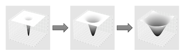
Figure 1: Example of BPs’ mitigation process. A flattened loss landscape ($1^{st}$ image), a.k.a. BPs, could be gradually recovered to the normal case ($3^{rd}$ image) by applying mitigation methods.

Numerous studies have been devoted to mitigating the barren plateau issues, whereas within these studies, initialization-based strategies have proven to be very effective by initializing qnns’ parameters with well-designed distributions Sack et al. (2022). However, most initialization-based strategies aim to mitigate BPs by one-time initialization with a well-designed data distribution, which may not be generalized to common data distribution. Initializing qnns’ parameters using deep-learning generative models could be a feasible solution since they can adaptively model data distribution on various datasets Friedrich and Maziero (2022). Within the category of generative models, large language models (llms) have demonstrated their superior performance in recent years Achiam et al. (2023); Dubey et al. (2024); Pham et al. (2024); Wang et al. (2024). Nonetheless, until now, leveraging the superior generative performance of llms to alleviate BPs is still under-explored.

To fill this research gap, we propose a new llm-driven framework, namely AdaInit, that can Adaptively generate Initial model parameters $\theta_{0}$ for qnns. After iterative generation, our framework obtains such an initial model parameter that can maximize the gradient variance for qnns’ training. Specifically, for each iteration, we estimate the posterior of $\theta_{0}$ using a generative model, such as a llm, given an adaptively improved prompt and a prior distribution as inputs. After posterior estimation, we train a qnn initialized with the generated $\theta_{0}$ and compute the gradient variance. We then evaluate the gradient variance by expected improvement (EI) and update the prompts if the EI is improved. Besides updating prompts, we store the corresponding $\theta_{0}$ and return the optimal one at the end. In this study, we theoretically analyze the submartingale property of EI and rigorously prove that the iterative search can eventually reach a supremum, which indicates that our framework can ultimately identify the optimal initial model parameters that maximize the gradient variance. Besides, we conduct extensive experiments to demonstrate the effectiveness of our proposed framework across four public datasets. The results reveal that our framework can maintain higher gradient variances against three classic initialization methods and two popular initialization-based strategies for mitigating BPs. Overall, we summarized our main primary contributions as follows:

• We propose a new llm-driven framework, AdaInit, for mitigating BPs. To the best of our knowledge, we first leverage llms to model qnns’ initial parameters for adaptively mitigating BPs.

• We theoretically analyze the submartingale property of expected improvement (EI) and rigorously prove the supremum of iterative search, providing theoretical validation for our search framework.

• Extensive experiments across four public datasets demonstrate that as the model size of qnns increases, our framework can maintain higher gradient variances against classic initialization methods.

2 Methodology

In this section, we first introduce the preliminary background and formally state the problem we aim to address in this study. Besides, we present our proposed framework in detail and conduct a theoretical analysis of the expected improvement (EI).

2.1 Preliminary Background

Variational Quantum Circuits (vqcs) play a core role in quantum neural networks (qnns). Typical vqcs consist of a finite sequence of unitary gates $U(\bm{\theta})$ parameterized by $\bm{\theta}\in\mathbb{R}^{LNR}$, where $L$, $N$, and $R$ denote the number of layers, qubits, and rotation gates. $U(\bm{\theta})$ can be formulated as:

$$U(\bm{\theta})=U(\theta_{1},...,\theta_{L})=\prod_{l=1}^{L}U_{l}(\theta_{l}),$$ (1)

where $U_{l}(\theta_{l})=e^{-i\theta_{l}V_{l}}$.

qnns, which are built by wrapping neural network layers with vqcs, can be optimized using gradient-based methods. To optimize qnns, we first define the loss function $E(\bm{\theta})$ of $U(\bm{\theta})$ as the expectation over Hermitian operator $H$:

$$E(\bm{\theta})=\langle 0|U(\bm{\theta})^{\dagger}HU(\bm{\theta})|0\rangle.$$ (2)

Given the loss function $E(\bm{\theta})$, we can further compute its gradient by the following formula:

$$\partial_{k}E\equiv\frac{\partial E(\bm{\theta})}{\partial\theta_{k}}=i\langle 0|U_{-}^{\dagger}\left[V_{k},U_{+}^{\dagger}HU_{+}\right]U_{-}|0\rangle,$$ (3)

where we denote $U_{-}\equiv\prod_{l=0}^{k-1}U_{l}(\theta_{l})W_{l}$ and $U_{+}\equiv\prod_{l=k}^{L}U_{l}(\theta_{l})W_{l}$. Also, $U(\bm{\theta})$ is sufficiently random s.t. both $U_{-}$ and $U_{+}$ (or either one) are independent and match the Haar distribution up to the second moment.

Barren Plateaus (BPs) are first investigated by McClean et al. (2018), who demonstrate that the gradient variance $\mathrm{Var}[\partial E]$ of qnns will exponentially decrease as the number of qubits $N$ increases when the random qnns match 2-design Haar distribution. This exponential pattern can be approximated as:

$$\mathrm{Var}[\partial E]\propto 2^{-2N}.$$ (4)

The Eq. 4 indicates that $\mathrm{Var}[\partial E]$ will approximate zero when the number of qubits $N$ is very large, i.e., most gradient-based approaches will fail to train qnns in this case.

Based on the above description, we formally state the problem that we aim to solve as follows:

Problem 1.

By leveraging a generative AI (GenAI) model, such as an llm, as a Bayesian posterior estimator with adaptive prompting, we aim to iteratively identify the optimal qnn’s parameter $\bm{\theta^{*}_{0}}$, where a given qnn is initialized with $\bm{\theta^{*}_{0}}$, which can maximize gradient variance $\mathrm{Var}[\partial E]$ during training, thereby mitigating barren plateaus (BPs).

2.2 Our Proposed Framework

In this study, we introduce a new framework, AdaInit, designed to mitigate BP issues in qnns by leveraging generative AI (GenAI) models, particularly llms. Our key innovations can be described as follows. (i) First, unlike conventional one-time initialization strategies, we propose a generative approach that iteratively searches the optimal initial model parameters $\bm{\theta^{*}_{0}}\in\mathbb{R}^{LNR}$ that maximize the gradient variance $\mathrm{Var}[\partial E]$ of qnns, thereby mitigating BPs and improving qnns’ trainability. In each search iteration, we employ an llm as a Bayesian estimator to refine the posterior (candidate initial model parameters $\bm{\theta_{0}}$) through adaptive prompting. After posterior estimation, we train the qnn initialized with the generated $\bm{\theta_{0}}$ and further compute its $\mathrm{Var}[\partial E]$. The benefit of using llm as a posterior estimator is that the llm can incorporate diverse textual instructions via prompts and adaptively update the prompts based on feedback from the previous iteration. This adaptive refinement allows our framework to dynamically optimize the generation process. (ii) To validate the generation quality, we employ Expected Improvement (EI), $\Delta^{(t)}$, as a guiding metric for our search. Furthermore, we rigorously prove that the EI and its cumulative sum satisfy the properties of submartingale. Consequently, we theoretically establish their boundedness, thereby demonstrating that our proposed search framework will ultimately find the optimal initial model parameters for qnns.

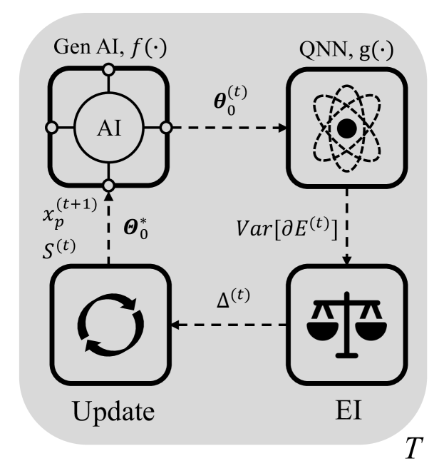
Figure 2: Our proposed framework follows an iterative search process over $T$ iterations (gray area). In $t$-th iteration, we perform four sequential steps: (i) Generate $\bm{\theta}_{0}^{(t)}$ using a Gen AI model, $f(\cdot)$, (ii) Compute $\mathrm{Var}[\partial E^{(t)}]$ after qnn’s training, (iii) Calculate EI, $\Delta^{(t)}$, and (iv) Update prompts $x_{p}^{(t+1)}$, historical maximum gradient variance $S^{(t)}$, and optimal candidates $\bm{\theta}_{0}^{*}$ for next iteration. Dashed arrows indicate data flow and corresponding outputs in each step.

Algorithm 1 Search for optimal initial model parameters for qnns.

0: A GenAI model $f(\cdot)$, prompts $x_{p}$, a qnn $g(\cdot)$, the number of search iterations $T$.

1: Initialize prompts $x_{p}$ and the GenAI model, $f(\cdot)$;

2: Create an empty list $\bm{\Theta}_{0}^{*}\leftarrow\varnothing$ to collect optimal candidates of initial model parameters for the qnn, $g(\cdot)$;

3: for $t=1$ to $T$ do

4:  $P(\bm{\theta}_{0}^{(t)}|x_{p}^{(t)})\leftarrow f(x_{p}^{(t)}|\bm{\theta}_{0}^{(t)})P(\bm{\theta}_{0}^{(t)})$;

5:  $\mathrm{Var}[\partial E^{(t)}]\leftarrow g(\bm{\theta}_{0}^{(t)})$;

6:  $\Delta^{(t)}\leftarrow\max(\mathrm{Var}[\partial E^{(t)}]-S^{(t-1)},0)$;

7:  if $\Delta^{(t)}>\frac{1}{poly(N,L)T}$ then

8:   $x_{p}^{(t+1)}\xleftarrow{\bm{\theta}_{0}^{(t)},\ \mathrm{Var}[\partial E^{(t)}],\ S^{(t-1)}}x_{p}^{(t)}$;

9:   $S^{(t)}\leftarrow\mathrm{Var}[\partial E^{(t)}]$;

10:   $\bm{\Theta}_{0}^{*}\leftarrow\bm{\Theta}_{0}^{*}\oplus[\bm{\theta}_{0}^{(t)}]$;

11:  end if

12: end for

13: return  $\bm{\Theta}_{0}^{*}$;

We present our framework workflow in Fig. 2 and further introduce details in Algo. 1. Given a GenAI model $f(\cdot)$, prompts $x_{p}$ for the $f(\cdot)$, a qnn $g(\cdot)$, and the number of search iterations $T$, we first initializes $f(\cdot)$, $x_{p}$ (line 1) and also creates an empty list $\varnothing$ for $\bm{\Theta}_{0}^{*}$ to collect optimal candidates of qnn’s initial model parameters (line 2). After initialization, we conduct $T$ iterations for searching (line 3). In each iteration, let’s say in the $t$-th iteration, we first employ $f(\cdot)$ with prompts $x_{p}^{(t)}$ and a prior distribution $P(\bm{\theta}_{0}^{(t)})$ to estimate the posterior distribution $P(\bm{\theta}_{0}^{(t)}|x_{p}^{(t)})$, which is the generated initial model parameter $\bm{\theta}_{0}^{(t)}$ for the qnn (line 4). After generation, we train the qnn $g(\bm{\theta}_{0}^{(t)})$ with certain training epochs and compute the gradient variance $\mathrm{Var}[\partial E^{(t)}]$, whose gradient is abbreviated from $\frac{\partial E(\bm{\theta}^{(t)})}{\partial\bm{\theta}^{(t)}}$, where $\bm{\theta}^{(t)}$ denotes the qnn’s model parameter in the $t$-th iteration (line 5). After computing the variance, we evaluate the improvement using the Expected Improvement (EI) metric, comparing the current gradient variance $\mathrm{Var}[\partial E^{(t)}]$ to the historical maximum gradient variance, which is the cumulative sum of EI when EI meets the following conditions (line 6). If the current EI, $\Delta^{(t)}$, is effectively improved, i.e., $\Delta^{(t)}>\frac{1}{poly(N,L)T}$, where $\frac{1}{poly(N,L)T}$ denotes a strictly positive lower bound on the gradient variance of an $N$-qubit, $L$-layer qnn for each search, in the absence of BPs (line 7), then we update the prompts for next iteration based on the current initial model parameters $\bm{\theta}_{0}^{(t)}$, the current gradient variance $\mathrm{Var}[\partial E^{(t)}]$, and the historical maximum gradient variance $S^{(t-1)}$ (line 8). After updating prompts, we update the historical maximum $S^{(t)}$ for the next iteration, where $S^{(t)}=S^{(t-1)}+\Delta^{(t)}=\mathrm{Var}[\partial E^{(t)}]$ (line 9) and further concatenate $\bm{\theta}_{0}^{(t)}$ to the optimal candidate list $\bm{\Theta}_{0}^{*}$ (line 10), which will be returned at the end (line 13). If so, the optimal initial model parameter $\bm{\theta}_{0}^{*}$ will be the last element in the candidate list.

Analysis of time and space complexity.

The search runs $T$ iterations. In each iteration, posterior estimation, which is linearly related to the output size of $\bm{\theta}_{0}$, takes $\mathcal{O}(|\bm{\theta}_{0}|)$ for a fixed-size qnn. Besides, training $g(\bm{\theta}_{0})$ with $T_{tr}$ epochs may take $\mathcal{O}(T_{tr}\cdot|\bm{\theta}_{0}|)$, where $T_{tr}$ denotes the number of training epochs for qnn. Combining $\bm{\theta}_{0}\in\mathbb{R}^{LNR}$, the total time complexity is $\mathcal{O}(T\cdot(L\cdot N\cdot R+T_{tr}\cdot L\cdot N\cdot R))\approx\mathcal{O}(T\cdot T_{tr}\cdot L\cdot N\cdot R)$. The space complexity primarily depends on the storage requirements. $\bm{\Theta}_{0}^{*}$ at most stores $T$ number of $\bm{\theta}_{0}$, which consumes $\mathcal{O}(T\cdot|\bm{\theta}_{0}|)$. The output of posterior estimation takes $\mathcal{O}(|\bm{\theta}_{0}|)$ space. Gradient variance and EI are scalars, which cost $\mathcal{O}(1)$ space. The prompts $x_{p}$ are iteratively updated and thus occupy $\mathcal{O}(|x_{p}|)$ space. Considering the size of $\bm{\theta}_{0}$, the total space complexity is $\mathcal{O}(T\cdot L\cdot N\cdot R+L\cdot N\cdot R+|x_{p}|)\approx\mathcal{O}(T\cdot L\cdot N\cdot R+|x_{p}|)$.

2.3 Theoretical Analysis of Expected Improvement (EI).

Before presenting the details of all necessary theoretical analysis, we would like to discuss how we can interpret these results. First, we formally define the Expected Improvement (EI) at each search iteration $t$ as $\Delta^{(t)}$ and its accumulative sum in the past iterations as $S^{(t-1)}$ in Def. 1. Besides, we assume that the maximum possible gradient $\partial E_{max}$ during qnn’s training is bounded by a positive constant $B_{\partial E}$, which is practical in real-world simulation. Next, we establish an upper bound for EI through Lem. 1 and Lem. 2. These results indicate that $S^{(t)}$ is $L^{1}$-bounded and integrable for each $t$. Building upon these lemmas, we investigate the submartingale property of $\Delta^{(t)}$ and rigorously prove in Lem. 3 that $S^{(t)}$ is submartingale. This insight is crucial as it provides a theoretical basis to analyze the convergence of our proposed search framework. Finally, leveraging the convergence of submartingales and the monotonicity of $S^{(t)}$, we establish in Lem. 4 that $S^{(t)}$ has a supremum, which indicates that our proposed search framework can eventually identify the optimal initial model parameters that maximize the gradient variance of qnns in optimization. Due to the page limit, we provide rigorous proof in the Appendix.

Definition 1 (Expected Improvement).

For $\forall$ $t\in\mathbb{Z}^{+}$, the Expected Improvement (EI) in the $t$-th search iteration is defined as:

$$\Delta^{(t)}=\max(\mathrm{Var}[\partial E^{(t)}]-S^{(t-1)},0),$$

where $\mathrm{Var}[\partial E^{(t)}]$ denotes the gradient variance in the $t$-th search iteration, and $S^{(t-1)}=\sum_{t_{i}=1}^{t-1}\Delta^{(t_{i})}\cdot I^{(t_{i})}$ denotes the maximum observed gradient variance in the past iterations, where $I^{(t_{i})}$ represents an indicator function $\mathbf{1}\bigl{(}\Delta^{(t_{i})}>\frac{1}{poly(N,L)T}\bigr{)}$ given a condition inside.

Assumption 1 (Bounded Maximum Gradient).

We assume there exists a positive constant $B_{\partial E}>0$, s.t. the maximum possible gradient $\partial E_{max}$ during qnn’s training satisfies:

$$\bigl{|}\partial E_{max}\bigr{|}\leq B_{\partial E}.$$

Without loss of generality, let’s say $\partial E_{max}\in[-\frac{B_{\partial E}}{2},\frac{B_{\partial E}}{2}]$.

Lemma 1 (Boundedness of Gradient Variance).

Given a certain-size quantum neural network (qnn), the variance of its gradient during training, $\mathrm{Var}[\partial E]$, is bounded by:

$$\mathrm{Var}[\partial E]\leq(\partial E_{\max}-\partial E_{\min})^{2},$$

where $\partial E_{\max}$ and $\partial E_{\min}$ denote the maximum and minimum values of the gradient $\partial E$, respectively.

Lemma 2 (Boundedness of EI).

From Def. 1 and Lem. 1, during the search of initial model parameters $\bm{\theta}_{0}$ for a certain-size qnn, for $\forall$ $t\in\mathbb{Z}^{+}$, there exist a bound for the expected improvement (EI) s.t.

$$\Delta^{(t)}\leq(\partial E_{max}-\partial E_{min})^{2}.$$

Lemma 3 (Submartingale Property of EI).

Let $\{\Delta^{(t)}\}_{t\geq 1}$ be an i.i.d. sequence of random variables on a probability space $(\Omega,\mathcal{F},P)$ s.t.

$$\begin{cases}P\bigl{(}\Delta^{(t)}>\frac{1}{poly(N,L)T}\bigr{)}=p,\\ P\bigl{(}\Delta^{(t)}\leq\frac{1}{poly(N,L)T}\bigr{)}=1-p,\end{cases}$$

for a probability $p\in[0,1]$. We define natural filtration $\mathcal{F}^{(t)}=\sigma\bigl{(}\Delta^{(1)},\Delta^{(2)},\dots,\Delta^{(t)}\bigr{)}$, and the selective accumulation of $\Delta^{(t)}$ for the past $t$ iteration as a stochastic process $\{S^{(t)}\}_{t\geq 1}$ according to Def. 1. Then, $\{S^{(t)}\}_{t\geq 1}$ is a submartingale with respect to the filtration $\{\mathcal{F}^{(t)}\}_{t\geq 1}$.

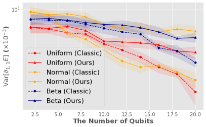
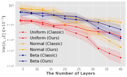
(a) Iris

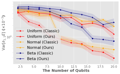
(b) Wine

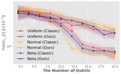
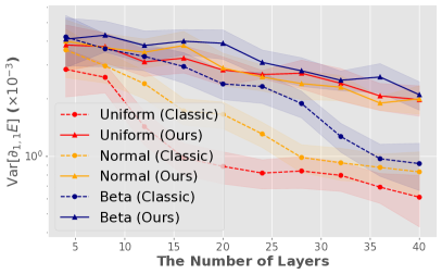
(c) Titanic

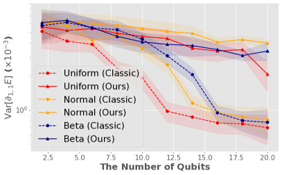
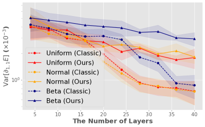
(d) MNIST

Figure 3: Analysis of gradient variance trends in the first element of qnns’ model parameters across varying qubit and layer settings for three classic initialization distributions, uniform, normal, and beta. “Classic” denotes that we initialize the model parameters with a classic distribution. “Ours” denotes that we use our framework to search the initial model parameters.

Lemma 4 (Boundedness of Submartingale).

Let $\{S^{(t)}\}_{t\geq 1}$ be a submartingale w.r.t. a $\{\mathcal{F}^{(t)}\}_{t\geq 1}$ s.t. $\sup_{t}\mathbb{E}[|S^{(t)}|]<\infty$. Then, $\{S^{(t)}\}_{t\geq 1}$ is almost surely bounded by a finite constant $B_{S}$ s.t.

$$S^{(t)}\leq B_{S},\quad\text{a.s.,}\quad\forall t\in\mathbb{Z}^{+}.$$

Table 1: Statistics of datasets. $\left|D\right|$, $\left|F\right|$, and $\left|C\right|$ denote the original number of instances, features, and classes, respectively. “Split” denotes the split instances for the train, validation, and test data.

Dataset	$\left|D\right|$	$\left|F\right|$	$\left|C\right|$	Splits
Iris	150	4	3	60:20:20
Wine	178	13	3	80:20:30
Titanic	891	11	2	320:80:179
MNIST	60,000	784	10	320:80:400

3 Experiment

In this section, we first introduce the experimental settings and further present our results in detail.

Dataset.

We evaluate our proposed method across four public datasets. Iris is a classic machine-learning benchmark that measures various attributes of three-species iris flowers. Wine is a well-known dataset that includes 13 attributes of chemical composition in wines. Titanic contains historical data about passengers aboard the Titanic and is typically used to predict the survival. MNIST is a widely used small benchmark in computer vision. This benchmark consists of 28$\times$28 gray-scale images of handwritten digits from 0 to 9. We follow the settings of BeInit Kulshrestha and Safro (2022) and conduct experiments in binary classification. Specifically, we sub-sample instances from the first two classes of each dataset to create a new subset. After sub-sampling, we adjust the feature dimensions to ensure they do not exceed the number of available qubits. The statistics of the original datasets, along with the data splits for training, validation, and testing, are presented in Table 1. Importantly, the total number of sub-sampled instances corresponds to the sum of the split datasets. For instance, in the Iris dataset, the total number of sub-sampled instances is 100.

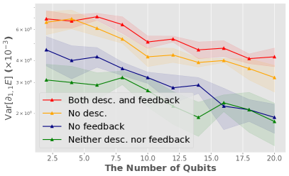
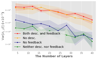
(a) Iris

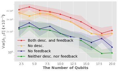
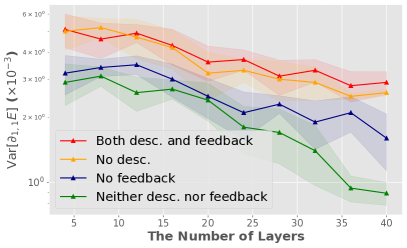
(b) Wine

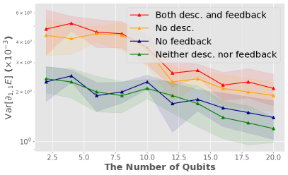
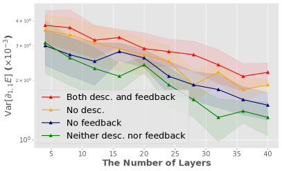
(c) Titanic

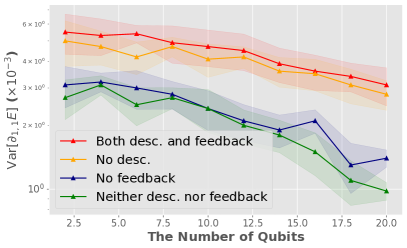
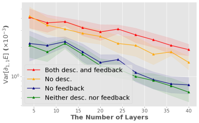
(d) MNIST

Figure 4: Analysis of prompts’ impact, i.e., investigate whether data description (desc.) and gradient feedback (feedback) affect the gradient variance in the first element of qnns’ model parameters across different model structures, considering variations in the number of qubits and layers.

Experimental settings.

In the experiment, we analyze the trend of gradient variance by varying the number of qubits ranging from 2 to 20 in increments of 2 (fixed 2 layers) and the number of layers spanning from 4 to 40 in steps of 4 (fixed 2 qubits). To obtain reliable results, we repeat the experiments five times and present them as curves (mean) with their bandwidth (standard deviation). During the search, our framework can identify the optimal model parameters within 50 iterations. In each search iteration, we employ the Adam optimizer with a learning rate of 0.01 and a batch size of 20 to train a qnn with 30 epochs and compute the gradient variance. After training, we compute the expected improvement (EI) and compare it with an assumed lower bound, $\frac{1}{poly(N,L)T}$, in each iteration. We compute the lower bound by $[2^{2N}T]^{-1}$, which is originally designed for uniform distribution. We empirically apply it for all cases as we observe in Fig. 3 that the magnitude of gradient variance is comparable across all datasets.

Evaluation.

We measure the qnn’s training by its gradient variance. A higher gradient variance in training indicates a lower likelihood of being trapped on the barren plateau landscape.

Figure 5: Example of three classic distributions commonly for initialization. In the figure, the red dots represent the initial values of the model parameters.

Searching initial model parameters of qnns via large language models can help alleviate barren plateaus.

We analyze gradient variance trends in the first element of qnns’ model parameters across varying qubit and layer settings for three classic initialization distributions, uniform, normal, and beta distributions, which are presented in Fig. 5 as examples. For each initialization with classic distribution, we compare it (“Classic”) with our proposed methods (“Ours”). As presented in Fig. 3, we observe that in the case of using classic initialization, the gradient variance of qnns will significantly decrease as the number of qubits or layers increases. Compared with it, our method can maintain higher variances, indicating that our framework can mitigate BPs better. In the rest of the experiments, if there is no specific state, we adopt uniform distribution as prior knowledge for posterior estimation.

Investigation of prompts.

We further examine whether the content of prompts influences search performance. In the experiments, we tested four prompting scenarios: (i) Including both data description and gradient feedback in prompts (Both desc. and feedback), (ii) Including gradient feedback only (No desc.), (iii) Including data description only (No feedback), (iv) Including neither data description nor gradient feedback (Neither desc. nor feedback). As the results presented in Fig. 4, we observe that suppressing either dataset description or gradient feedback in the prompts leads to a reduction in the gradient variance of qnns. Notably, the reduction is more significant in most cases when gradient feedback is muted compared to the dataset description, suggesting that both factors play a crucial role in mitigating BPs, with gradient feedback contributing significantly more.

llms	Acc.	Max i/o
GPT 4o	100%	128K/4K
GPT 4o mini	85%	128K/16K
Gemini 1.5 flash	75%	1M/8K
Gemini 1.5 pro	90%	2M/8K
Claude 3.5 sonnet	100%	200K/8K

Table 2: Comparison of initial model parameters’ generation by accuracy (Acc.) using llms, GPT Hurst et al. (2024), Gemini Team et al. (2024), and Claude Anthropic (2024). We measure the generation under different numbers of qubits and layers (20 combinations in total). We also present the maximum number of input/output tokens in the third column.

Comparison of generative performance using llms.

In our proposed framework, the initial model parameters of qnns are generated by llms. In this experiment, we compare the generative performance under varying qnn structures, such as different numbers of qubits or layers. Specifically, we primarily evaluate whether the correct size of model parameters can be generated by testing 20 combinations in accuracy, fixing either 2 layers while varying qubits from 2 to 20 or 2 qubits while varying layers from 4 to 40. As shown in Tab. 2, the results indicate that both GPT-4o and Claude 3.5 Sonnet can achieve 100% accuracy in generating the correct shapes of model parameters. Considering that 4K output tokens are sufficient for our settings, in this study, we mainly use GPT 4o as the backbone llms.

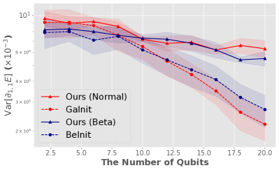
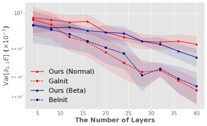
Figure 6: Comparison between two initialization-based strategies, GaInit and BeInit, and our framework, which is initialized with corresponding data distribution for a fair comparison.

Comparison with initialization-based strategies.

We compare our framework with two popular initialization-based strategies, GaInit Zhang et al. (2022) and BeInit Kulshrestha and Safro (2022). Both of them leverage well-designed Normal and Beta distributions to initialize the quantum circuits, respectively. For a fair comparison, we initialize the qnns with the corresponding distribution. We present the results on Iris in Fig. 6 as an example. The results demonstrate that our framework can identify the initial model parameters of qnns that achieve higher gradient variance during training as the model size increases, indicating better mitigation for BPs.

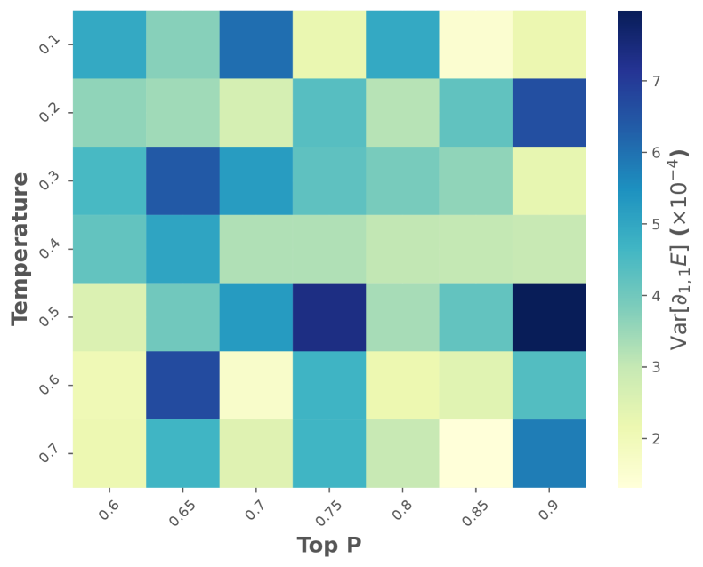
(a) Iris

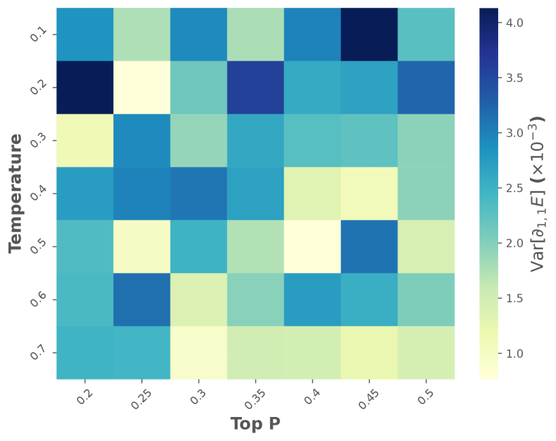
(b) Wine

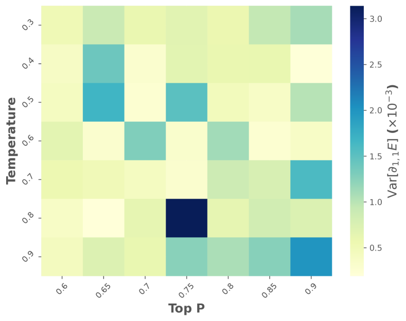
(c) Titanic

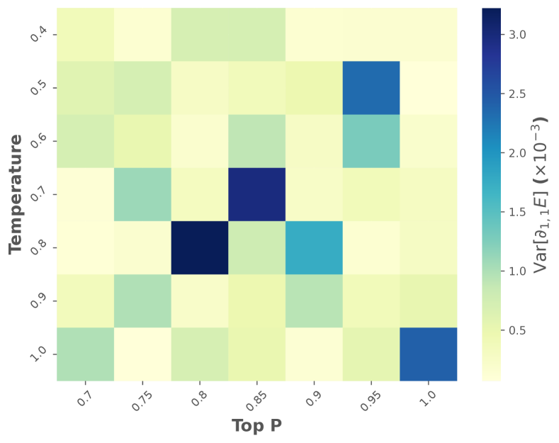
(d) MNIST

Figure 7: Analysis of the sensitivity of hyperparameters, including Temperature and Top P. The grid with the darkest color indicates the optimal combination.

Sensitivity analysis of hyperparameters.

We analyze the sensitivity of hyperparameters, including Temperature and Top P, for llms. Temperature controls the randomness of predictions, with higher values generating more diverse outputs, while Top P affects the probabilities of token selections, ensuring a more focused yet flexible generation. To identify the optimal settings, we first narrowed down the hyperparameter ranges through manual tuning and then applied grid search to determine the best combinations (Temperature, Top P) for each dataset: Iris (0.5, 0.9), Wine (0.1, 0.45), Titanic (0.8, 0.75), and MNIST (0.8, 0.8), as presented in Fig. 7. The combinations of the above hyperparameters were subsequently used in this study.

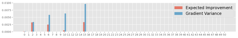
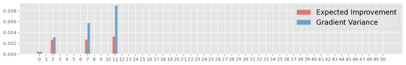
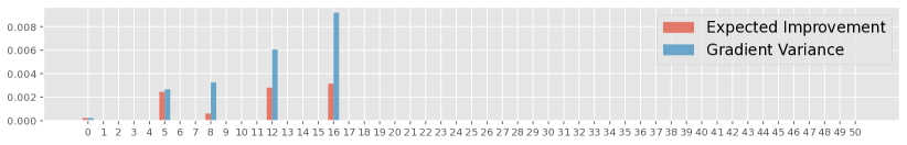
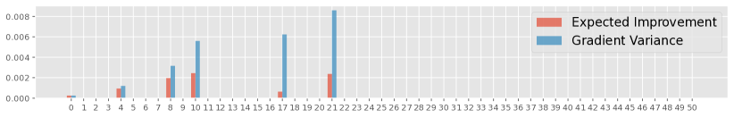
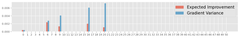
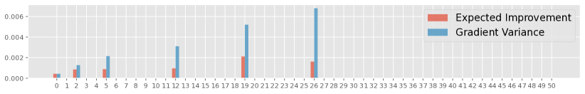
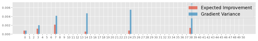
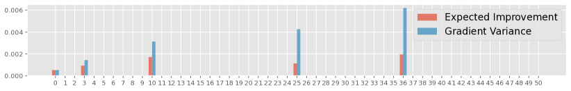
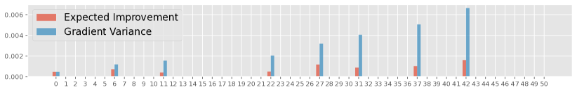
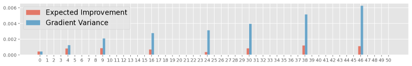
(a) The number of qubits ranges from 2 to 20.

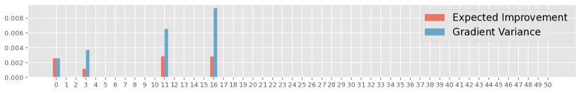
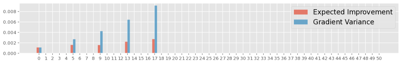
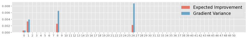
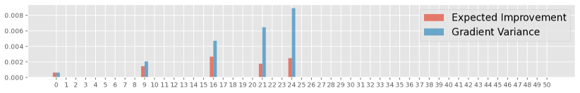
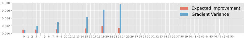
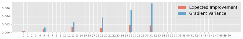
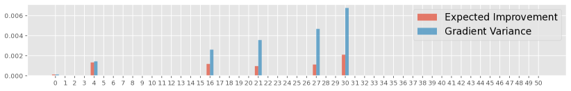
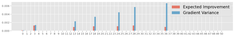
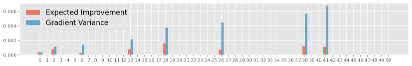
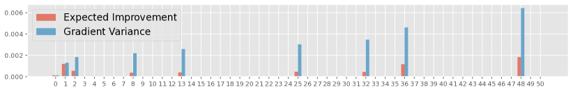
(b) The number of layers ranges from 4 to 40.

Figure 8: We analyze the patterns of expected improvement and the corresponding gradient variance and present the results in two columns: the left column illustrates the trends w.r.t. the number of qubits, while the right column captures the effects of increasing the number of layers.

Analysis of the expected improvement.

We analyze the patterns on the expected improvement (EI) and the corresponding gradient variance across various qnn structures as search iterations progress. Representative experiments conducted on Iris are illustrated in Fig. 8 as an example. Our findings show that as the model size grows, more search iterations are required to obtain optimal initial parameters that enable qnns to maintain higher gradient variance in training. This is expected, as larger models expand the search space, demanding greater computational resources to explore effectively.

4 Related Work

McClean et al. (2018) first investigated barren plateau (BP) phenomenons and demonstrated that under the assumption of the 2-design Haar distribution, gradient variance in qnns will exponentially decrease to zero during training as the model size increases. In recent years, enormous studies have been devoted to mitigating BP issues in qnns Qi et al. (2023). Cunningham and Zhuang (2024) categorize most existing studies into the following five groups. (i) Initialization-based strategies initialize model parameters with various well-designed distributions in the initialization stage Grant et al. (2019); Sack et al. (2022); Mele et al. (2022); Grimsley et al. (2023); Liu et al. (2023); Park and Killoran (2024). (ii) Optimization-based strategies address BP issues and further enhance trainability during optimization Ostaszewski et al. (2021); Suzuki et al. (2021); Heyraud et al. (2023); Liu et al. (2024); Sannia et al. (2024). (iii) Model-based strategies attempt to mitigate BPs by proposing new model architectures Li et al. (2021); Bharti and Haug (2021); Du et al. (2022); Selvarajan et al. (2023); Tüysüz et al. (2023); Kashif and Al-Kuwari (2024). (iv) To address both BPs and saddle points, Zhuang et al. (2024) regularize qnns’ model parameters via Bayesian approaches. (v) Rappaport et al. (2023) measure BP phenomenon via various informative metrics.

5 Conclusion

In this study, we proposed a new llm-driven framework, AdaInit, designed to mitigate barren plateaus (BPs) in qnn’s training. By iteratively refining qnn’s initialization through adaptive prompting and posterior estimation, AdaInit can maximize gradient variance, improving qnn’s trainability against BPs. Our theoretical analysis establishes the submartingale property of expected improvement (EI), ensuring the iterative search can eventually identify optimal initial model parameters for qnn. Through extensive experiments across four public datasets, we demonstrated that AdaInit outperforms conventional classic initialization methods in maintaining higher gradient variance as qnn’s sizes increase. Overall, this study paves a new way to explore how llms help mitigate BPs in qnn’s training.

Limitations & future work.

First, in our theoretical analysis, we assume that the maximum gradient of qnns is bounded by a positive constant, i.e., the gradient doesn’t explode during training. This assumption is practical in most cases. Besides, we rigorously prove that the submartingale has a supremum in our settings. In the future, we plan to prove that convergence of submartingale is guaranteed in a finite number of search iterations.

Appendix A APPENDIX

In the appendix, we present the architecture of the quantum circuit and our hardware/software. Besides, we display the prompt designs in this study.

Model architecture of the quantum circuit.

In this study, we examine our proposed framework using a backbone qnn, which concatenates the following quantum circuit with a fully connected layer. The circuit architecture is described in Figure 9.

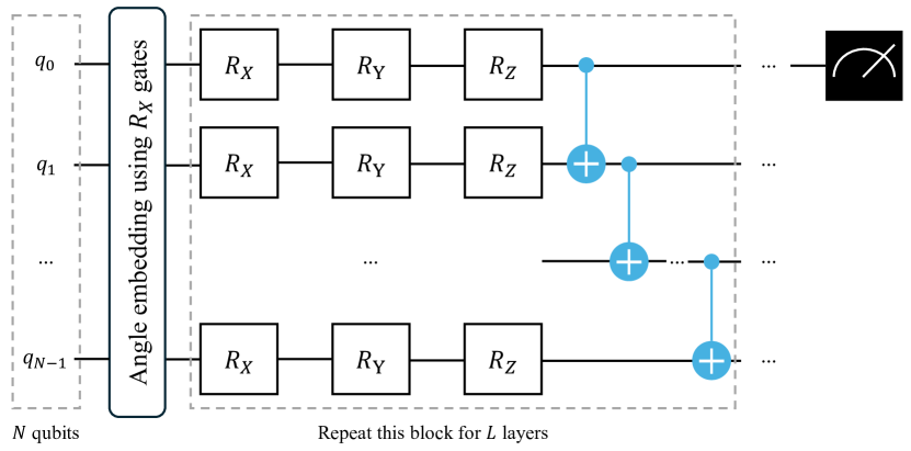
Figure 9: Architecture of our backbone quantum circuit. The number of rotation gates in this study is fixed as 3.

Hardware and software.

The experiment is conducted on a server with the following settings:

• Operating System: Ubuntu 22.04.3 LTS

• CPU: Intel Xeon w5-3433 @ 4.20 GHz

• GPU: NVIDIA RTX A6000 48GB

• Software: Python 3.11, PyTorch 2.1, Pennylane 0.31.1.

Prompt designs.

Before presenting the prompts, we first introduce the notation for the hyperparameter in prompts. ‘nlayers’, ‘nqubits’, ‘nrot’, ‘nclasses’ denote the number of layers, qubits, rotation gates, and classes for the qnn, respectively. ‘init’ denotes the initial data distribution for the qnn. ‘data_desc’ denotes the data description. ‘feedback’ denotes the gradient feedback from the previous iteration during the search.

Proof of Lemmas.

We provide a rigorous proof of the following lemmas.

Lem. 1.

We denote a sequence of gradient $\bm{\partial E}=\{\partial E^{(t)}\}_{t=0}^{T_{tr}}$, where $T_{tr}$ represents the number of training epochs for a qnn. Within this sequence, we denote $\partial E_{max}$, $\partial E_{min}$, and $\overline{\partial E}$ as the maximum, minimum, and mean values of the gradient. For $\forall$ $t\in\mathbb{Z}^{+}$, we have:

$$\partial E^{(t)},\overline{\partial E}\in[\partial E_{min},\partial E_{max}],$$

then the gap between $\partial E^{(t)}$ and $\overline{\partial E}$ will not exceed the range of $[\partial E_{min},\partial E_{max}]$:

$$|\partial E^{(t)}-\overline{\partial E}|\leq\partial E_{max}-\partial E_{min}.$$

Thus, we have:

$$\mathrm{Var}[\partial E] =\frac{1}{T_{tr}}\sum_{t=1}^{T_{tr}}(\partial E^{(t)}-\overline{\partial E})^{2}$$

$$\leq\frac{1}{T_{tr}}\sum_{t=1}^{T_{tr}}(\partial E_{max}-\partial E_{min})^{2}$$

$$=(\partial E_{max}-\partial E_{min})^{2}.$$

Thus, the gradient variance $\mathrm{Var}[\partial E]$ satisfies the bound $\mathrm{Var}[\partial E]\leq(\partial E_{max}-\partial E_{min})^{2}$. ∎

Lem. 2.

From Def. 1, for $\forall$ $t\in\mathbb{Z}^{+}$, in the $t$-th search iteration, we have:

$$\Delta^{(t)}=\max(\mathrm{Var}[\partial E^{(t)}]-S^{(t-1)},0).$$

Combining with Lem. 1, for $\forall$ $t\in\mathbb{Z}^{+}$, we have:

$$\mathrm{Var}[\partial E^{(t)}],S^{(t-1)}\leq(\partial E_{max}-\partial E_{min})^{2}.$$

The above equation holds true as $S^{(t-1)}$ denotes the historical maximum gradient variance in the past iterations. Thus, we have:

$$\mathrm{Var}[\partial E^{(t)}]-S^{(t-1)}\leq(\partial E_{max}-\partial E_{min})^{2},$$

which indicates that:

$$\Delta^{(t)}\leq(\partial E_{max}-\partial E_{min})^{2}.$$

∎

Lem. 3.

A process $S^{(t)}$ is submartingale relative to $(\Omega,\mathcal{F},P)$ if the following three conditions, Adaptedness, Integrability, and Submartingale condition, hold true Williams (1991).

Adaptedness.

We first aim to verify that $S^{(t)}$ is determined based on the information available up to past $t$ iterations. By Def. 1, $S^{(t)}=\sum_{t_{i}=1}^{t}\Delta^{(t_{i})}\cdot I^{(t_{i})}$ is a finite sum of random variables that are measurable w.r.t. $\sigma\bigl{(}\Delta^{(1)},\Delta^{(2)},\dots,\Delta^{(t)}\bigr{)}$. Thus, $S^{(t)}$ is also measurable w.r.t. $\mathcal{F}^{(t)}$, ensuring the adaptedness.

Integrability.

In Lem. 2, $\Delta^{(t)}\leq(\partial E_{max}-\partial E_{min})^{2}$ for $\forall$ $t\in\mathbb{Z}^{+}$. Thus,

$$\mathbb{E}[|S^{(t)}|] =\mathbb{E}\Bigl{[}\Bigl{|}\sum_{t_{i}=1}^{t}\Delta^{(t_{i})}\cdot I^{(t_{i})}\Bigr{|}\Bigr{]}$$

$$\leq\mathbb{E}\Bigl{[}\Bigl{|}\sum_{t_{i}=1}^{t}(\partial E_{max}-\partial E_{min})^{2}\cdot I^{(t_{i})}\Bigr{|}\Bigr{]}$$

$$<\infty,$$

which ensures $\mathbb{E}[|S^{(t)}|]$ is integrable for each $t$.

Submartingale condition.

We observe that

$$S^{(t)}=S^{(t-1)}+\Delta^{(t)}.$$

Thus, given $\mathcal{F}^{(t-1)}$, we have

$$\mathbb{E}\bigl{[}S^{(t)}\big{|}\mathcal{F}^{(t-1)}\bigr{]}=\mathbb{E}\bigl{[}S^{(t-1)}+\Delta^{(t)}\big{|}\mathcal{F}^{(t-1)}\bigr{]},$$

Since $S^{(t-1)}$ is $\mathcal{F}^{(t-1)}$-measurable and $\{\Delta^{(t)}\}_{t\geq 1}$ is i.i.d., thus,

$$\mathbb{E}\bigl{[}S^{(t)}\big{|}\mathcal{F}^{(t-1)}\bigr{]} =\mathbb{E}\bigl{[}S^{(t-1)}+\Delta^{(t)}\big{|}\mathcal{F}^{(t-1)}\bigr{]}$$

$$=S^{(t-1)}+\mathbb{E}[\Delta^{(t)}]$$

$$=S^{(t-1)}+\bigl{(}\delta p+0(1-p)\bigr{)}$$

$$\geq S^{(t-1)},$$

where $\delta$ denotes a positive increment when $\Delta^{(t)}>\frac{1}{poly(N,L)T}$.

Thus, the submartingale condition holds true for $\forall$ $t\geq 1$ s.t.

$$\mathbb{E}\bigl{[}S^{(t)}\big{|}\mathcal{F}^{(t-1)}\bigr{]}\geq S^{(t-1)},\quad\forall t\geq 1,$$

∎

Lem. 4.

Since the process $\{S^{(t)}\}_{t\geq 1}$ is a $L^{1}$-bounded submartingale s.t. $\sup_{t}\mathbb{E}[|S^{(t)}|]<\infty$, we apply Doob’s Forward Convergence Theorem Williams (1991), which guarantees the almost sure existence of a finite random variable $S^{(\infty)}$ s.t. $S^{(\infty)}$=$\lim_{t\to\infty}S^{(t)}$. This implies that the process $\{S^{(t)}\}$ has a well-defined almost sure limit.

Furthermore, if $\{S^{(t)}\}$ is monotone increasing, i.e., $S^{(t)}\leq S^{(t+1)}$, a.s., $\forall$ $t\in\mathbb{Z}^{+}$, then the limit $S^{(\infty)}$ serves as a supremum for the entire process. By Defining $B_{S}:=\sup_{t}S^{(t)}=S^{(\infty)}$, we obtain a desired bound $S^{(t)}\leq B_{S}$, a.s., $\forall$ $t\in\mathbb{Z}^{+}$. ∎

Computational budgets.

Based on the above computing infrastructure and settings, computational budgets in our experiments are described as follows. Our search framework can be reproduced within one hour given that the number of qubits is less than 18. The total experiments take around 600 hours to complete.

Ethical and broader impacts.

We confirm that we fulfill the author’s responsibilities and address the potential ethical issues. This work paves a novel way to explore how generative models, such as llms, help improve the trainability of qnns, which could benefit the community of natural language processing and quantum machine learning.

Statement of data privacy.

The datasets used in this study were obtained from publicly available sources.

Potential risk.

Reproducing the experiments in this study may take significant time and computational resources.

Disclaimer regarding human subjects results.

NA

References

- Achiam et al. (2023) Josh Achiam, Steven Adler, Sandhini Agarwal, Lama Ahmad, Ilge Akkaya, Florencia Leoni Aleman, Diogo Almeida, Janko Altenschmidt, Sam Altman, Shyamal Anadkat, et al. 2023. Gpt-4 technical report. arXiv preprint arXiv:2303.08774.
- Anthropic (2024) Anthropic. 2024. Introducing claude 3.5 sonnet. Accessed: 2025-02-15.
- Bharti and Haug (2021) Kishor Bharti and Tobias Haug. 2021. Quantum-assisted simulator. Physical Review A, 104(4):042418.
- Chen et al. (2022) Samuel Yen-Chi Chen, Tzu-Chieh Wei, Chao Zhang, Haiwang Yu, and Shinjae Yoo. 2022. Quantum convolutional neural networks for high energy physics data analysis. Physical Review Research, 4(1):013231.
- Cunningham and Zhuang (2024) Jack Cunningham and Jun Zhuang. 2024. Investigating and mitigating barren plateaus in variational quantum circuits: A survey. arXiv preprint arXiv:2407.17706.
- Du et al. (2022) Yuxuan Du, Tao Huang, Shan You, Min-Hsiu Hsieh, and Dacheng Tao. 2022. Quantum circuit architecture search for variational quantum algorithms. npj Quantum Information, 8(1):62.
- Dubey et al. (2024) Abhimanyu Dubey, Abhinav Jauhri, Abhinav Pandey, Abhishek Kadian, Ahmad Al-Dahle, Aiesha Letman, Akhil Mathur, Alan Schelten, Amy Yang, Angela Fan, et al. 2024. The llama 3 herd of models. arXiv preprint arXiv:2407.21783.
- Friedrich and Maziero (2022) Lucas Friedrich and Jonas Maziero. 2022. Avoiding barren plateaus with classical deep neural networks. Physical Review A, 106(4):042433.
- Grant et al. (2019) Edward Grant, Leonard Wossnig, Mateusz Ostaszewski, and Marcello Benedetti. 2019. An initialization strategy for addressing barren plateaus in parametrized quantum circuits. Quantum.
- Grimsley et al. (2023) Harper R Grimsley, George S Barron, Edwin Barnes, Sophia E Economou, and Nicholas J Mayhall. 2023. Adaptive, problem-tailored variational quantum eigensolver mitigates rough parameter landscapes and barren plateaus. npj Quantum Information, 9(1):19.
- Heyraud et al. (2023) Valentin Heyraud, Zejian Li, Kaelan Donatella, Alexandre Le Boité, and Cristiano Ciuti. 2023. Efficient estimation of trainability for variational quantum circuits. PRX Quantum, 4(4):040335.
- Hurst et al. (2024) Aaron Hurst, Adam Lerer, Adam P Goucher, Adam Perelman, Aditya Ramesh, Aidan Clark, AJ Ostrow, Akila Welihinda, Alan Hayes, Alec Radford, et al. 2024. Gpt-4o system card. arXiv preprint arXiv:2410.21276.
- Kashif and Al-Kuwari (2024) Muhammad Kashif and Saif Al-Kuwari. 2024. Resqnets: a residual approach for mitigating barren plateaus in quantum neural networks. EPJ Quantum Technology.
- Kulshrestha and Safro (2022) Ankit Kulshrestha and Ilya Safro. 2022. Beinit: Avoiding barren plateaus in variational quantum algorithms. In 2022 IEEE international conference on quantum computing and engineering (QCE), pages 197–203. IEEE.
- Li et al. (2021) Guangxi Li, Zhixin Song, and Xin Wang. 2021. Vsql: Variational shadow quantum learning for classification. In Proceedings of the AAAI conference on artificial intelligence.
- Liang et al. (2024) Zhiding Liang, Jinglei Cheng, Hang Ren, Hanrui Wang, Fei Hua, Zhixin Song, Yongshan Ding, Frederic T Chong, Song Han, Xuehai Qian, et al. 2024. Napa: intermediate-level variational native-pulse ansatz for variational quantum algorithms. IEEE Transactions on Computer-Aided Design of Integrated Circuits and Systems.
- Liang et al. (2023) Zhiding Liang, Jinglei Cheng, Rui Yang, Hang Ren, Zhixin Song, Di Wu, Xuehai Qian, Tongyang Li, and Yiyu Shi. 2023. Unleashing the potential of llms for quantum computing: A study in quantum architecture design. arXiv preprint arXiv:2307.08191.
- Liu et al. (2023) Huan-Yu Liu, Tai-Ping Sun, Yu-Chun Wu, Yong-Jian Han, and Guo-Ping Guo. 2023. Mitigating barren plateaus with transfer-learning-inspired parameter initializations. New Journal of Physics, 25(1):013039.
- Liu et al. (2024) Xia Liu, Geng Liu, Hao-Kai Zhang, Jiaxin Huang, and Xin Wang. 2024. Mitigating barren plateaus of variational quantum eigensolvers. IEEE Transactions on Quantum Engineering.
- McClean et al. (2018) Jarrod R McClean, Sergio Boixo, Vadim N Smelyanskiy, Ryan Babbush, and Hartmut Neven. 2018. Barren plateaus in quantum neural network training landscapes. Nature communications, 9(1):4812.
- Mele et al. (2022) Antonio A Mele, Glen B Mbeng, Giuseppe E Santoro, Mario Collura, and Pietro Torta. 2022. Avoiding barren plateaus via transferability of smooth solutions in a hamiltonian variational ansatz. Physical Review A, 106(6):L060401.
- Ostaszewski et al. (2021) Mateusz Ostaszewski, Edward Grant, and Marcello Benedetti. 2021. Structure optimization for parameterized quantum circuits. Quantum, 5:391.
- Park and Killoran (2024) Chae-Yeun Park and Nathan Killoran. 2024. Hamiltonian variational ansatz without barren plateaus. Quantum, 8:1239.
- Pham et al. (2024) Bach Pham, JuiHsuan Wong, Samuel Kim, Yunting Yin, and Steven Skiena. 2024. Word definitions from large language models.
- Preskill (2018) John Preskill. 2018. Quantum computing in the nisq era and beyond. Quantum, 2:79.
- Qi et al. (2023) Han Qi, Lei Wang, Hongsheng Zhu, Abdullah Gani, and Changqing Gong. 2023. The barren plateaus of quantum neural networks: review, taxonomy and trends. Quantum Information Processing, 22(12):435.
- Rappaport et al. (2023) Sonny Rappaport, Gaurav Gyawali, Tiago Sereno, and Michael J Lawler. 2023. Measurement-induced landscape transitions in hybrid variational quantum circuits. arXiv preprint arXiv:2312.09135.
- Sack et al. (2022) Stefan H Sack, Raimel A Medina, Alexios A Michailidis, Richard Kueng, and Maksym Serbyn. 2022. Avoiding barren plateaus using classical shadows. PRX Quantum, 3(2):020365.
- Sannia et al. (2024) Antonio Sannia, Francesco Tacchino, Ivano Tavernelli, Gian Luca Giorgi, and Roberta Zambrini. 2024. Engineered dissipation to mitigate barren plateaus. npj Quantum Information, 10(1):81.
- Selvarajan et al. (2023) Raja Selvarajan, Manas Sajjan, Travis S Humble, and Sabre Kais. 2023. Dimensionality reduction with variational encoders based on subsystem purification. Mathematics.
- Stein et al. (2021) Samuel A Stein, Betis Baheri, Daniel Chen, Ying Mao, Qiang Guan, Ang Li, Bo Fang, and Shuai Xu. 2021. Qugan: A quantum state fidelity based generative adversarial network. In 2021 IEEE International Conference on Quantum Computing and Engineering (QCE), pages 71–81. IEEE.
- Suzuki et al. (2021) Yudai Suzuki, Hiroshi Yano, Rudy Raymond, and Naoki Yamamoto. 2021. Normalized gradient descent for variational quantum algorithms. In 2021 IEEE International Conference on Quantum Computing and Engineering (QCE), pages 1–9. IEEE.
- Team et al. (2024) Gemini Team, Petko Georgiev, Ving Ian Lei, Ryan Burnell, Libin Bai, Anmol Gulati, Garrett Tanzer, Damien Vincent, Zhufeng Pan, Shibo Wang, et al. 2024. Gemini 1.5: Unlocking multimodal understanding across millions of tokens of context. arXiv preprint arXiv:2403.05530.
- Tüysüz et al. (2023) Cenk Tüysüz, Giuseppe Clemente, Arianna Crippa, Tobias Hartung, Stefan Kühn, and Karl Jansen. 2023. Classical splitting of parametrized quantum circuits. Quantum Machine Intelligence.
- Wang et al. (2024) Zuhui Wang, Yunting Yin, and IV Ramakrishnan. 2024. Enhancing image-text matching with adaptive feature aggregation. In ICASSP 2024-2024 IEEE International Conference on Acoustics, Speech and Signal Processing (ICASSP), pages 8245–8249. IEEE.
- Williams (1991) David Williams. 1991. Probability with martingales. Cambridge university press.
- Zhang et al. (2022) Kaining Zhang, Liu Liu, Min-Hsiu Hsieh, and Dacheng Tao. 2022. Escaping from the barren plateau via gaussian initializations in deep variational quantum circuits. Advances in Neural Information Processing Systems.
- Zhuang et al. (2024) Jun Zhuang, Jack Cunningham, and Chaowen Guan. 2024. Improving trainability of variational quantum circuits via regularization strategies. arXiv preprint arXiv:2405.01606.