RAD: Training an End-to-End Driving Policy via Large-Scale 3DGS-based Reinforcement Learning

Abstract

Existing end-to-end autonomous driving (AD) algorithms typically follow the Imitation Learning (IL) paradigm, which faces challenges such as causal confusion and the open-loop gap. In this work, we establish a 3DGS-based closed-loop Reinforcement Learning (RL) training paradigm. By leveraging 3DGS techniques, we construct a photorealistic digital replica of the real physical world, enabling the AD policy to extensively explore the state space and learn to handle out-of-distribution scenarios through large-scale trial and error. To enhance safety, we design specialized rewards that guide the policy to effectively respond to safety-critical events and understand real-world causal relationships. For better alignment with human driving behavior, IL is incorporated into RL training as a regularization term. We introduce a closed-loop evaluation benchmark consisting of diverse, previously unseen 3DGS environments. Compared to IL-based methods, RAD achieves stronger performance in most closed-loop metrics, especially $3\times$ lower collision rate. Abundant closed-loop results are presented at https://hgao-cv.github.io/RAD.

1 Introduction

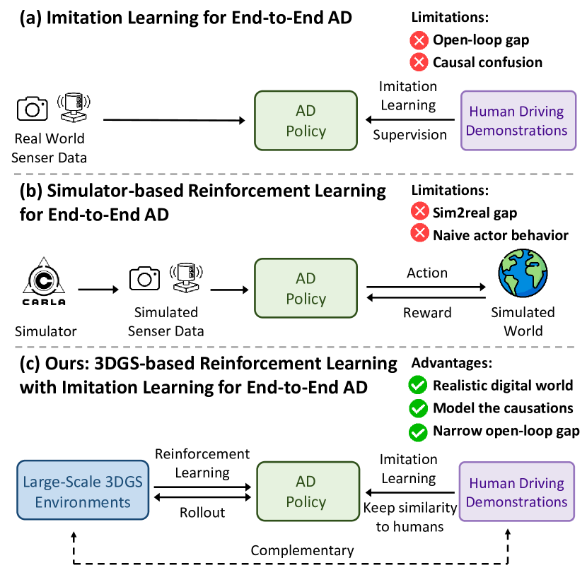
Figure 1: Different training paradigms of end-to-end autonomous driving (AD).

End-to-end autonomous driving (AD) is currently a trending topic in both academia and industry. It replaces a modularized pipeline with a holistic one by directly mapping sensory inputs to driving actions, offering advantages in system simplicity and generalization ability. Most existing end-to-end AD algorithms [11, 17, 49, 43, 22, 2, 38, 28] follow the Imitation Learning (IL) paradigm, which trains a neural network to mimic human driving behavior. However, despite their simplicity, IL-based methods face significant challenges in real-world deployment.

One key issue is causal confusion. IL trains a network to replicate human driving policies by learning from demonstrations. However, this paradigm primarily captures correlations rather than causal relationships between observations (states) and actions. As a result, IL-trained policies may struggle to identify the true causal factors behind planning decisions, leading to shortcut learning [8], e.g., merely extrapolating future trajectories from historical ones [23, 47]. Furthermore, since IL training data predominantly consists of common driving behaviors and does not adequately cover long-tailed distributions, IL-trained policies tend to converge to trivial solutions, lacking sufficient sensitivity to safety-critical events such as collisions.

Another major challenge is the gap between open-loop training and closed-loop deployment. IL policies are trained in an open-loop manner using well-distributed driving demonstrations. However, real-world driving is a closed-loop process where minor trajectory errors at each step accumulate over time, leading to compounding errors and out-of-distribution scenarios. IL-trained policies often struggle in these unseen situations, raising concerns about their robustness.

A straightforward solution to these problems is to perform closed-loop Reinforcement Learning (RL) training, which requires a driving environment that can interact with the AD policy. However, using real-world driving environments for closed-loop training poses prohibitive safety risks and operational costs. Simulated driving environments with sensor data simulation capabilities [6, 14] (which are required for end-to-end AD) are typically built on game engines [7, 39] but fail to provide realistic sensor simulation results.

In this work, we establish a 3DGS-based [18] closed-loop RL training paradigm. Leveraging 3DGS techniques, we construct a photorealistic digital replica of the real world, where the AD policy can extensively explore the state space and learn to handle out-of-distribution situations through large-scale trial and error. To ensure effective responses to safety-critical events and a better understanding of real-world causations, we design specialized safety-related rewards. However, RL training presents several critical challenges, which this paper addresses.

One significant challenge is the Human Alignment Problem. The exploration process in RL can lead to policies that deviate from human-like behavior, disrupting the smoothness of the action sequence. To address this, we incorporate imitation learning as a regularization term during RL training, helping to maintain similarity to human driving behavior. As illustrated in Fig. 1, RL and IL work together to optimize the AD policy: RL enhances IL by addressing causation and the open-loop gap, while IL improves RL by ensuring better human alignment.

Another major challenge is the Sparse Reward Problem. RL often suffers from sparse rewards and slow convergence. To alleviate this issue, we introduce dense auxiliary objectives related to collisions and deviations, which help constrain the full action distribution. Additionally, we streamline and decouple the action space to reduce the exploration cost associated with RL.

To validate the effectiveness of our approach, we construct a closed-loop evaluation benchmark comprising diverse, unseen 3DGS environments. Our method, RAD, outperforms IL-based approaches across most closed-loop metrics, notably achieving a collision rate that is $3\times$ lower.

The contributions of this work are summarized as follows:

• We propose the first 3DGS-based RL framework for training end-to-end AD policy. The reward, action space, optimization objective, and interaction mechanism are specially designed to enhance training efficiency and effectiveness.

• We combine RL and IL to synergistically optimize the AD policy. RL complements IL by modeling the causations and narrowing the open-loop gap, while IL complements RL in terms of human alignment.

• We validate the effectiveness of RAD on a closed-loop evaluation benchmark consisting of diverse, unseen 3DGS environments. RAD achieves stronger performance in closed-loop evaluation, particularly a $3\times$ lower collision rate, compared to IL-based methods.

2 Related Work

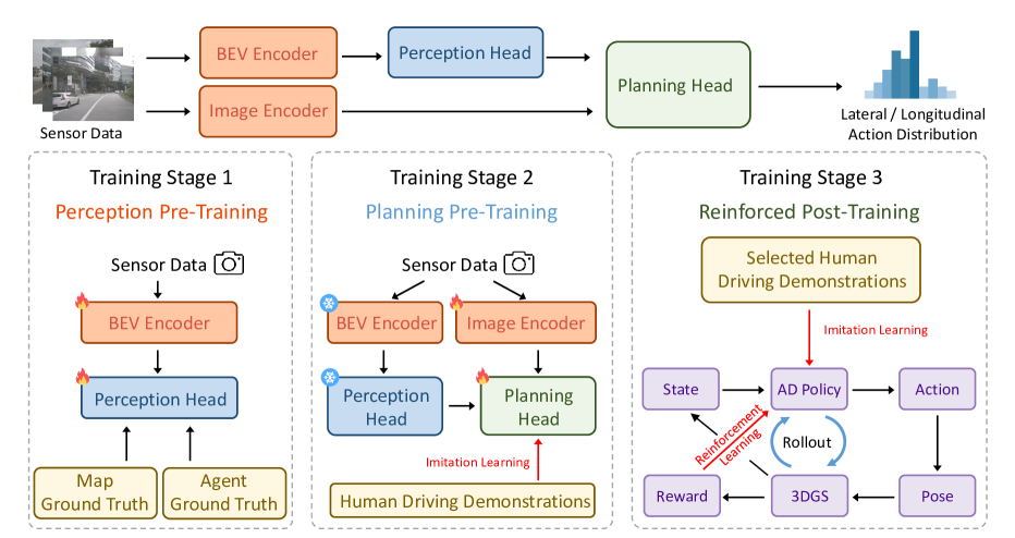
Figure 2: Overall framework of RAD. RAD takes a three-stage training paradigm. In the perception pre-training, ground-truths of map and agent are used to guide instance-level tokens to encode corresponding information. In the planning pre-training stage, large-scale driving demonstrations are used to initialize the action distribution. In the reinforced post-training stage, RL and IL synergistically fine-tune the AD policy.

Dynamic Scene Reconstruction. Implicit neural representations have dominated novel view synthesis and dynamic scene reconstruction, with methods like UniSim [46], MARS [44], and NeuRAD [40] leveraging neural scene graphs to enable structured scene decomposition. However, these approaches rely on implicit representations, leading to slow rendering speeds that limit their practicality in real-time applications. In contrast, 3D Gaussian Splatting (3DGS) [18] has emerged as an efficient alternative, offering significantly faster rendering while maintaining high visual fidelity. Recent works have explored its potential for dynamic scene reconstruction, particularly in autonomous driving scenarios. StreetGaussians [45], DrivingGaussians [51], and HUGSIM [50] have demonstrated the effectiveness of Gaussian-based representations in modeling urban environments. These methods achieve superior rendering performance while maintaining controllability by explicitly decomposing scenes into structured components. However, these works primarily leverage 3DGS for closed-loop evaluation. In this work, we incorporate 3DGS into an RL training framework.

End-to-End Autonomous Driving. Learning-based planning has shown great potential recently due to its data-driven nature and impressive performance with increasing amounts of data. UniAD [12] demonstrates the potential of end-to-end autonomous driving by integrating multiple perception tasks to enhance planning performance. VAD [16] further explores the use of compact vectorized scene representations to improve efficiency. A series of works [20, 43, 49, 24, 42, 9, 3, 33] also adopt the single-trajectory planning paradigm and further enhance planning performance. VADv2 [2] shifts the paradigm towards multi-mode planning by modeling the probabilistic distribution of a planning vocabulary. Hydra-MDP [22] improves the scoring mechanism of VADv2 by introducing additional supervision from a rule-based scorer. SparseDrive [38] explores an alternative BEV-free solution. DiffusionDrive [28] proposes a truncated diffusion policy that denoises an anchored Gaussian distribution to a multi-mode driving action distribution. Most of the end-to-end methods follow the data-driven IL-training paradigm. In this work, we present an RL-training paradigm based on 3DGS.

Reinforcement Learning. Reinforcement Learning is a promising technique that has not been fully explored. AlphaGo [36] and AlphaGo Zero [37] have demonstrated the power of Reinforcement Learning in the game of Go. Recently, OpenAI O1 [32] and Deepseek-R1 [4] have leveraged Reinforcement Learning to develop reasoning abilities. Several studies have also applied Reinforcement Learning in autonomous driving [41, 1, 48, 31, 13]. However, these studies are based on non-photorealistic simulators (such as CARLA [6]) or do not involve end-to-end driving algorithms, as they require perfect perception results as input. To the best of our knowledge, RAD is the first work to train an end-to-end AD agent using Reinforcement Learning in a photorealistic 3DGS environment.

3 RAD

3.1 End-to-End Driving Policy

The overall framework of RAD is depicted in Fig. 2. RAD takes multi-view image sequences as input, transforms the sensor data into scene token embeddings, outputs the probabilistic distribution of actions, and samples an action to control the vehicle.

BEV Encoder. We first employ a BEV encoder [21] to transform multi-view image features from the perspective view to the Bird’s Eye View (BEV), obtaining a feature map in the BEV space. This feature map is then used to learn instance-level map features and agent features.

Map Head. Then we utilize a group of map tokens [27, 25, 26] to learn the vectorized map elements of the driving scene from the BEV feature map, including lane centerlines, lane dividers, road boundaries, arrows, traffic signals, etc.

Agent Head. Besides, a group of agent tokens [15] is adopted to predict the motion information of other traffic participants, including location, orientation, size, speed, and multi-mode future trajectories.

Image Encoder. Apart from the above instance-level map and agent tokens, we also use an individual image encoder [5, 10] to transform the original images into image tokens. These image tokens provide dense and rich scene information for planning, complementary to the instance-level tokens.

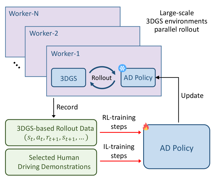
Figure 3: Post-training. $N$ workers parallelly run. The generated rollout data $(s_{t},a_{t},r_{t+1},s_{t+1},...)$ are recorded in a rollout buffer. Rollout data and human driving demonstrations are used in RL- and IL-training steps to fine-tune the AD policy synergistically.

Action Space. To accelerate the convergence of RL training, we design a decoupled discrete action representation. We divide the action into two independent components: lateral action and longitudinal action. The action space is constructed over a short $0.5$-second time horizon, during which the vehicle’s motion is approximated by assuming constant linear and angular velocities. Under this assumption, the lateral action $a^{x}$ and longitudinal action $a^{y}$ can be directly computed based on the current linear and angular velocities. By combining decoupling with a limited temporal scope and simplified motion model, our approach effectively reduces the dimensionality of the action space, accelerating training convergence.

Planning Head. We use $E_{\text{scene}}$ to denote the scene representation, which consists of map tokens, agent tokens, and image tokens. We initialize a planning embedding denoted as $E_{\text{plan}}$. A cascaded Transformer decoder $\phi$ takes the planning embedding $E_{\text{plan}}$ as the query and the scene representation $E_{\text{scene}}$ as both key and value.

The output of the decoder $\phi$ is then combined with navigation information $E_{\text{navi}}$ and ego state $E_{\text{state}}$ to output the probabilistic distributions of the lateral action $a^{x}$ and the longitudinal action $a^{y}$:

$$\pi(a^{x}\mid s)= \text{softmax}(\text{MLP}(\phi(E_{\text{plan}},E_{\text{scene}})$$ (1)

$$+E_{\text{navi}}+E_{\text{state}})),$$

$$\pi(a^{y}\mid s)= \text{softmax}(\text{MLP}(\phi(E_{\text{plan}},E_{\text{scene}})$$

$$+E_{\text{navi}}+E_{\text{state}})),$$

where $E_{\text{plan}}$, $E_{\text{navi}}$, $E_{\text{state}}$, and the output of MLP are all of the same dimension ($1\times D$).

The planning head also outputs the value functions $V_{x}(s)$ and $V_{y}(s)$, which estimate the expected cumulative rewards for the lateral and longitudinal actions, respectively:

$$V_{x}(s)=\text{MLP}(\phi(E_{\text{plan}},E_{\text{scene}})+E_{\text{navi}}+E_{\text{state}}),$$ (2)

$$V_{y}(s)=\text{MLP}(\phi(E_{\text{plan}},E_{\text{scene}})+E_{\text{navi}}+E_{\text{state}}).$$

The value functions are used in RL training (Sec. 3.5).

3.2 Training Paradigm

We adopt a three-stage training paradigm: perception pre-training, planning pre-training, and reinforced post-training, as shown in Fig. 2.

Perception Pre-Training. Information in the image is sparse and low-level. In the first stage, the map head and the agent head explicitly output map elements and agent motion information, which are supervised with ground-truth labels. Consequently, map tokens and agent tokens implicitly encode the corresponding high-level information. In this stage, we only update the parameters of the BEV encoder, the map head, and the agent head.

Planning Pre-Training. In the second stage, to prevent the unstable cold start of RL training, IL is first performed to initialize the probabilistic distribution of actions based on large-scale real-world driving demonstrations from expert drivers. In this stage, we only update the parameters of the image encoder and the planning head, while the parameters of the BEV encoder, map head, and agent head are frozen. The optimization objectives of perception tasks and planning tasks may conflict with each other. However, with the training stage and parameters decoupled, such conflicts are mostly avoided.

Reinforced Post-Training. In the reinforced post-training, RL and IL synergistically fine-tune the distribution. RL aims to guide the policy to be sensitive to critical risky events and adaptive to out-of-distribution situations. IL serves as the regularization term to keep the policy’s behavior similar to that of humans.

We select a large amount of risky dense-traffic clips from collected driving demonstrations. For each clip, we train an independent 3DGS model that reconstructs the clip and serves as a digital driving environment. As shown in Fig. 3, we set $N$ parallel workers. Each worker randomly samples a 3DGS environment and begins rollout, i.e., the AD policy controls the ego vehicle to move and iteratively interacts with the 3DGS environment. After the rollout process of this 3DGS environment ends, the generated rollout data $(s_{t},a_{t},r_{t+1},s_{t+1},...)$ are recorded in a rollout buffer, and the worker will sample a new 3DGS environment for another round of rollout.

As for policy optimization, we iteratively perform RL-training steps and IL-training steps. For RL-training steps, we sample data from the rollout buffer and follow the Proximal Policy Optimization (PPO) framework [35] to update the AD policy. For IL-training steps, we use real-world driving demonstrations to update the policy. After a fixed number of training steps, the updated AD policy is sent to every worker to replace the old one, to avoid a distribution shift between data collection and optimization. We only update the parameters of the image encoder and the planning head. The parameters of the BEV encoder, the map head, and the agent head are frozen. The detailed RL design is presented below.

3.3 Interaction Mechanism between AD Policy and 3DGS Environment

In the 3DGS environment, the ego vehicle acts according to the AD policy. Other traffic participants act according to real-world data in a log-replay manner. A simplified kinematic bicycle model is employed to iteratively update the ego vehicle’s pose at every $\Delta t$ seconds as follows:

$$x_{t+1}^{w} =x_{t}^{w}+v_{t}\cos\left(\psi_{t}^{w}\right)\Delta t,$$ (3)

$$y_{t+1}^{w} =y_{t}^{w}+v_{t}\sin\left(\psi_{t}^{w}\right)\Delta t,$$

$$\psi_{t+1}^{w} =\psi_{t}^{w}+\frac{v_{t}}{L}\tan\left(\delta_{t}\right)\Delta t,$$

where $x_{t}^{w}$ and $y_{t}^{w}$ denote the position of the ego vehicle relative to the world coordinate; $\psi_{t}^{w}$ is the heading angle that defines the vehicle’s orientation with respect to the world $x$-coordinate; $v_{t}$ is the linear velocity of the ego vehicle; $\delta_{t}$ is the steering angle of the front wheels; and $L$ is the wheelbase, i.e., the distance between the front and rear axles.

During the rollout process, the AD policy outputs actions $(a_{t}^{x},a_{t}^{y})$ for a $0.5$-second time horizon at time step $t$. We derive the linear velocity $v_{t}$ and steering angle $\delta_{t}$ based on $(a_{t}^{x},a_{t}^{y})$. Based on the kinematic model in Eq. 3, the pose of the ego vehicle in the world coordinate system is updated from ${p}_{t}=(x_{t}^{w},y_{t}^{w},\psi_{t}^{w})$ to ${p}_{t+1}=(x_{t+1}^{w},y_{t+1}^{w},\psi_{t+1}^{w})$.

Based on the updated ${p}_{t+1}$, the 3DGS environment computes the new ego vehicle’s state $s_{t+1}$. The updated pose ${p}_{t+1}$ and state $s_{t+1}$ serve as the input for the next iteration of the inference process.

The 3DGS environment also generates rewards $\mathcal{R}$ (Sec. 3.4) according to multi-source information (including trajectories of other agents, map information, the expert trajectory of the ego vehicle, and the parameters of Gaussians), which are used to optimize the AD policy (Sec. 3.5).

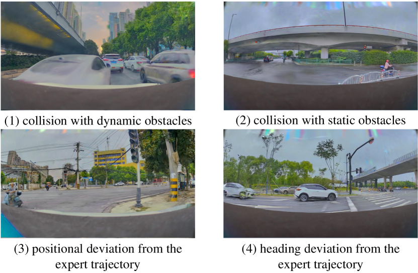
Figure 4: Example diagram of four types of reward sources. (1): Collision with a dynamic obstacle ahead triggers a reward $r_{\text{dc}}$. (2): Hitting a static roadside obstacle incurs a reward $r_{\text{sc}}$. (3): Moving onto the curb exceeds the positional deviation threshold $d_{\text{max}}$, triggering a reward $r_{\text{pd}}$. (4): Drifting toward the adjacent lane exceeds the heading deviation threshold $\psi_{\text{max}}$, triggering a reward $r_{\text{hd}}$.

3.4 Reward Modeling

The reward is the source of the training signal, which determines the optimization direction of RL. The reward function is designed to guide the ego vehicle’s behavior by penalizing unsafe actions and encouraging alignment with the expert trajectory. It is composed of four reward components: (1) collision with dynamic obstacles, (2) collision with static obstacles, (3) positional deviation from the expert trajectory, and (4) heading deviation from the expert trajectory:

$$\mathcal{R}=\{r_{\text{dc}},r_{\text{sc}},r_{\text{pd}},r_{\text{hd}}\}.$$ (4)

As illustrated in Fig. 4, these reward components are triggered under specific conditions. In the 3DGS environment, dynamic collision is detected if the ego vehicle’s bounding box overlaps with the annotated bounding boxes of dynamic obstacles, triggering a negative reward $r_{\text{dc}}$. Similarly, static collision is identified when the ego vehicle’s bounding box overlaps with the Gaussians of static obstacles, resulting in a negative reward $r_{\text{sc}}$. Positional deviation is measured as the Euclidean distance between the ego vehicle’s current position and the closest point on the expert trajectory. A deviation beyond a predefined threshold $d_{\text{max}}$ incurs a negative reward $r_{\text{pd}}$. Heading deviation is calculated as the angular difference between the ego vehicle’s current heading angle $\psi_{t}$ and the expert trajectory’s matched heading angle $\psi_{\text{expert}}$. A deviation beyond a threshold $\psi_{\text{max}}$ results in a negative reward $r_{\text{hd}}$.

Any of these events, including dynamic collision, static collision, excessive positional deviation, or excessive heading deviation, triggers immediate episode termination. Because after such events occur, the 3DGS environment typically generates noisy sensor data, which is detrimental to RL training.

3.5 Policy Optimization

In the closed-loop environment, the error in each single step accumulates over time. The aforementioned rewards are not only caused by the current action but also by the actions of the preceding steps. The rewards are propagated forward with Generalized Advantage Estimation (GAE) [34] to optimize the action distribution of the preceding steps.

Specifically, for each time step $t$, we store the current state $s_{t}$, action $a_{t}$, reward $r_{t}$, and the estimate of the value $V(s_{t})$. Based on the decoupled action space, and considering that different rewards have different correlations to lateral and longitudinal actions, the reward $r_{t}$ is divided into lateral reward $r_{t}^{x}$ and longitudinal reward $r_{t}^{y}$:

$$r_{t}^{x} =r_{t}^{\text{sc}}+r_{t}^{\text{pd}}+r_{t}^{\text{hd}},$$ (5)

$$r_{t}^{y} =r_{t}^{\text{dc}}.$$

Similarly, the value function $V(s_{t})$ is decoupled into two components: $V_{x}(s_{t})$ for the lateral dimension and $V_{y}(s_{t})$ for the longitudinal dimension. These value functions estimate the expected cumulative rewards for the lateral and longitudinal actions, respectively. The advantage estimates $\hat{A}_{t}^{x}$ and $\hat{A}_{t}^{y}$ are then computed as follows:

$$\delta_{t}^{x} =r_{t}^{x}+\gamma V_{x}(s_{t+1})-V_{x}(s_{t}),$$ (6)

$$\delta_{t}^{y} =r_{t}^{y}+\gamma V_{y}(s_{t+1})-V_{y}(s_{t}),$$

$$\hat{A}_{t}^{x} =\sum_{l=0}^{\infty}(\gamma\lambda)^{l}\delta_{t+l}^{x},$$

$$\hat{A}_{t}^{y} =\sum_{l=0}^{\infty}(\gamma\lambda)^{l}\delta_{t+l}^{y},$$

where $\delta_{t}^{x}$ and $\delta_{t}^{y}$ are the temporal difference errors for the lateral and longitudinal dimensions, $\gamma$ is the discount factor, and $\lambda$ is the GAE parameter that controls the trade-off between bias and variance.

To further clarify the relationship between the advantage estimates and the reward components, we decompose $\hat{A}_{t}^{x}$ and $\hat{A}_{t}^{y}$ based on the reward decomposition in Eq. 5 and the advantage estimation in Eq. 6. Specifically, we derive the following decomposition:

$$\hat{A}_{t}^{x} =\hat{A}_{t}^{\text{sc}}+\hat{A}_{t}^{\text{pd}}+\hat{A}_{t}^{\text{hd}},$$ (7)

$$\hat{A}_{t}^{y} =\hat{A}_{t}^{\text{dc}},$$

where $\hat{A}_{t}^{\text{sc}}$ is the advantage estimate for avoiding static collisions, $\hat{A}_{t}^{\text{pd}}$ is the advantage estimate for minimizing positional deviations, $\hat{A}_{t}^{\text{hd}}$ is the advantage estimate for minimizing heading deviations, and $\hat{A}_{t}^{\text{dc}}$ is the advantage estimate for avoiding dynamic collisions.

These advantage estimates are used to guide the update of the AD policy $\pi_{\theta}$, following the PPO framework [35]. By leveraging the decomposed advantage estimates $\hat{A}_{t}^{x}$ and $\hat{A}_{t}^{y}$, we can independently optimize the lateral and longitudinal dimensions of the policy. This is achieved by defining separate objective functions $\mathcal{L}_{x}^{\text{CLIP}}(\theta)$ and $\mathcal{L}_{y}^{\text{CLIP}}(\theta)$ for each dimension, as follows:

$$\mathcal{L}_{x}^{\text{PPO}}(\theta) =\mathbb{E}_{t}\left[\min\left(\rho_{t}^{x}\hat{A}_{t}^{x},\ \text{clip}(\rho_{t}^{x},1-\epsilon_{x},1+\epsilon_{x})\hat{A}_{t}^{x}\right)\right],$$ (8)

$$\mathcal{L}_{y}^{\text{PPO}}(\theta) =\mathbb{E}_{t}\left[\min\left(\rho_{t}^{y}\hat{A}_{t}^{y},\ \text{clip}(\rho_{t}^{y},1-\epsilon_{y},1+\epsilon_{y})\hat{A}_{t}^{y}\right)\right],$$

$$\mathcal{L}^{\text{PPO}}(\theta) =\mathcal{L}_{x}^{\text{PPO}}(\theta)+\mathcal{L}_{y}^{\text{PPO}}(\theta),$$

where $\rho_{t}^{x}=\frac{\pi_{\theta}(a_{t}^{x}\mid s_{t})}{\pi_{\theta_{\text{old}}}(a_{t}^{x}\mid s_{t})}$ is the importance sampling ratio for the lateral dimension, $\rho_{t}^{y}=\frac{\pi_{\theta}(a_{t}^{y}\mid s_{t})}{\pi_{\theta_{\text{old}}}(a_{t}^{y}\mid s_{t})}$ is the importance sampling ratio for the longitudinal dimension, $\epsilon_{x}$ and $\epsilon_{y}$ are small constants that control the clipping range for the lateral and longitudinal dimensions, ensuring stable policy updates.

The clipped objective function $\mathcal{L}^{\text{PPO}}(\theta)$ prevents excessively large updates to the policy parameters $\theta$, thereby maintaining training stability.

RL:IL	CR$\downarrow$	DCR$\downarrow$	SCR$\downarrow$	DR$\downarrow$	PDR$\downarrow$	HDR$\downarrow$	ADD$\downarrow$	Long. Jerk$\downarrow$	Lat. Jerk$\downarrow$
0:1	0.229	0.211	0.018	0.066	0.039	0.027	0.238	3.928	0.103
1:0	0.143	0.128	0.015	0.080	0.065	0.015	0.345	4.204	0.085
2:1	0.137	0.125	0.012	0.059	0.050	0.009	0.274	4.538	0.092
4:1	0.089	0.080	0.009	0.063	0.042	0.021	0.257	4.495	0.082
8:1	0.125	0.116	0.009	0.084	0.045	0.039	0.323	5.285	0.115

Table 1: Ablation on RL-to-IL step mixing ratios in the reinforced post-training stage.

3.6 Auxiliary Objective

RL usually faces the challenge of sparse rewards, which makes the convergence process unstable and slow. To speed up convergence, we introduce auxiliary objectives that provide dense guidance to the entire action distribution.

The auxiliary objectives are designed to penalize undesirable behaviors by incorporating specific reward sources, including dynamic collisions, static collisions, positional deviations, and heading deviations. These objectives are computed based on the actions $a_{t}^{x,\text{old}}$ and $a_{t}^{y,\text{old}}$ selected by the old AD policy $\pi_{\theta_{\text{old}}}$ at time step $t$. To facilitate the evaluation of these actions, we separate the probability distribution of the action into four parts:

$$\Delta\pi_{y}^{\text{dec}} =\sum_{a_{t}^{y}<a_{t}^{y,\text{old}}}\pi_{\theta}(a_{t}^{y}\mid s_{t}),$$ (9)

$$\Delta\pi_{y}^{\text{acc}} =\sum_{a_{t}^{y}>a_{t}^{y,\text{old}}}\pi_{\theta}(a_{t}^{y}\mid s_{t}),$$

$$\Delta\pi_{x}^{\text{left}} =\sum_{a_{t}^{x}<a_{t}^{x,\text{old}}}\pi_{\theta}(a_{t}^{x}\mid s_{t}),$$

$$\Delta\pi_{x}^{\text{right}} =\sum_{a_{t}^{x}>a_{t}^{x,\text{old}}}\pi_{\theta}(a_{t}^{x}\mid s_{t}).$$

Here, $\Delta\pi_{y}^{\text{dec}}$ represents the total probability of deceleration actions, $\Delta\pi_{y}^{\text{acc}}$ represents the total probability of acceleration actions, $\Delta\pi_{x}^{\text{left}}$ represents the total probability of leftward steering actions, and $\Delta\pi_{x}^{\text{right}}$ represents the total probability of rightward steering actions.

Dynamic Collision Auxiliary Objective. The dynamic collision auxiliary objective adjusts the longitudinal control action $a_{t}^{y}$ based on the location of potential collisions relative to the ego vehicle. If a collision is detected ahead, the policy prioritizes deceleration actions ($a_{t}^{y}<a_{t}^{y,\text{old}}$); if a collision is detected behind, it encourages acceleration actions ($a_{t}^{y}>a_{t}^{y,\text{old}}$). To formalize this behavior, we define a directional factor $f_{\text{dc}}$:

$$f_{\text{dc}}=\begin{cases}1&\text{if the collision is ahead},\\ -1&\text{if the collision is behind}.\end{cases}$$ (10)

The auxiliary objective for dynamic collision avoidance is defined as:

$$\mathcal{L}_{\text{dc}}(\theta_{y})=\mathbb{E}_{t}\left[\hat{A}_{t}^{\text{dc}}\cdot f_{\text{dc}}\cdot(\Delta\pi_{y}^{\text{dec}}-\Delta\pi_{y}^{\text{acc}})\right],$$ (11)

where $\hat{A}_{t}^{\text{dc}}$ is the advantage estimate for dynamic collision avoidance.

Static Collision Auxiliary Objective. The static collision auxiliary objective adjusts the steering control action $a_{t}^{x}$ based on the proximity to static obstacles. If the static obstacle is detected on the left side, the policy promotes rightward steering actions ($a_{t}^{x}>a_{t}^{x,\text{old}}$); if the static obstacle is detected on the right side, it promotes leftward steering actions ($a_{t}^{x}<a_{t}^{x,\text{old}}$). To formalize this behavior, we define a directional factor $f_{\text{sc}}$:

$$f_{\text{sc}}=\begin{cases}1&\text{if static obstacle is on the left},\\ -1&\text{if static obstacle is on the right}.\end{cases}$$ (12)

The auxiliary objective for static collision avoidance is defined as:

$$\mathcal{L}_{\text{sc}}(\theta_{x})=\mathbb{E}_{t}\left[\hat{A}_{t}^{\text{sc}}\cdot f_{\text{sc}}\cdot(\Delta\pi_{x}^{\text{right}}-\Delta\pi_{x}^{\text{left}})\right],$$ (13)

where $\hat{A}_{t}^{\text{sc}}$ is the advantage estimate for static collision avoidance.

Positional Deviation Auxiliary Objective. The positional deviation auxiliary objective adjusts the steering control action $a_{t}^{x}$ based on the ego vehicle’s lateral deviation from the expert trajectory. If the ego vehicle deviates leftward, the policy promotes rightward corrections ($a_{t}^{x}>a_{t}^{x,\text{old}}$); if it deviates rightward, it promotes leftward corrections ($a_{t}^{x}<a_{t}^{x,\text{old}}$). We formalize this with a directional factor $f_{\text{pd}}$:

$$f_{\text{pd}}=\begin{cases}1&\text{if ego vehicle deviates leftward},\\ -1&\text{if ego vehicle deviates rightward}.\end{cases}$$ (14)

The auxiliary objective for positional deviation correction is:

$$\mathcal{L}_{\text{pd}}(\theta_{x})=\mathbb{E}_{t}\left[\hat{A}_{t}^{\text{pd}}\cdot f_{\text{pd}}\cdot(\Delta\pi_{x}^{\text{right}}-\Delta\pi_{x}^{\text{left}})\right],$$ (15)

where $\hat{A}_{t}^{\text{pd}}$ estimates the advantage of trajectory alignment.

Heading Deviation Auxiliary Objective. The heading deviation auxiliary objective adjusts the steering control action $a_{t}^{x}$ based on the angular difference between the ego vehicle’s current heading and the expert’s reference heading. If the ego vehicle deviates counterclockwise, the policy promotes clockwise corrections ($a_{t}^{x}>a_{t}^{x,\text{old}}$); if it deviates clockwise, it promotes counterclockwise corrections ($a_{t}^{x}<a_{t}^{x,\text{old}}$). To formalize this behavior, we define a directional factor $f_{\text{hd}}$:

$$f_{\text{hd}}=\begin{cases}1&\text{if ego vehicle deviates clockwise},\\ -1&\text{if ego vehicle deviates counterclockwise}.\end{cases}$$ (16)

The auxiliary objective for heading deviation correction is then defined as:

$$\mathcal{L}_{\text{hd}}(\theta_{x})=\mathbb{E}_{t}\left[\hat{A}_{t}^{\text{hd}}\cdot f_{\text{hd}}\cdot(\Delta\pi_{x}^{\text{right}}-\Delta\pi_{x}^{\text{left}})\right],$$ (17)

where $\hat{A}_{t}^{\text{hd}}$ is the advantage estimate for heading alignment.

ID	Dynamic	Static	Position	Heading	CR$\downarrow$	DCR$\downarrow$	SCR$\downarrow$	DR$\downarrow$	PDR$\downarrow$	HDR$\downarrow$	ADD$\downarrow$	Long. Jerk$\downarrow$	Lat. Jerk$\downarrow$
	Collision	Collision	Deviation	Deviation
1	✓				0.172	0.154	0.018	0.092	0.033	0.059	0.259	4.211	0.095
2		✓	✓	✓	0.238	0.217	0.021	0.090	0.045	0.045	0.241	3.937	0.098
3	✓		✓	✓	0.146	0.128	0.018	0.060	0.030	0.030	0.263	3.729	0.083
4	✓	✓		✓	0.151	0.142	0.009	0.069	0.042	0.027	0.303	3.938	0.079
5	✓	✓	✓		0.166	0.157	0.009	0.048	0.036	0.012	0.243	3.334	0.067
6	✓	✓	✓	✓	0.089	0.080	0.009	0.063	0.042	0.021	0.257	4.495	0.082

Table 2: Ablation on reward sources. The table shows the impact of different reward components on performance.

ID	PPO Obj.	Dynamic Col.	Static Col.	Position Dev.	Heading Dev.	CR$\downarrow$	DCR$\downarrow$	SCR$\downarrow$	DR$\downarrow$	PDR$\downarrow$	HDR$\downarrow$	ADD$\downarrow$	Long. Jerk$\downarrow$	Lat. Jerk$\downarrow$
		Auxiliary Obj.	Auxiliary Obj.	Auxiliary Obj.	Auxiliary Obj.
1	✓					0.249	0.223	0.026	0.077	0.047	0.030	0.266	4.209	0.104
2	✓	✓				0.178	0.163	0.015	0.151	0.101	0.050	0.301	3.906	0.085
3	✓		✓	✓	✓	0.137	0.125	0.012	0.157	0.145	0.012	0.296	3.419	0.071
4	✓	✓		✓	✓	0.169	0.151	0.018	0.075	0.042	0.033	0.254	4.450	0.098
5	✓	✓	✓		✓	0.149	0.134	0.015	0.063	0.057	0.006	0.324	3.980	0.086
6	✓	✓	✓	✓		0.128	0.119	0.009	0.066	0.030	0.036	0.254	4.102	0.092
7		✓	✓	✓	✓	0.187	0.175	0.012	0.077	0.056	0.021	0.309	5.014	0.112
8	✓	✓	✓	✓	✓	0.089	0.080	0.009	0.063	0.042	0.021	0.257	4.495	0.082

Table 3: Ablation on auxiliary objectives. The table shows the impact of different auxiliary objectives on performance.

Overall Auxiliary Objectives. The overall auxiliary objectives are a weighted sum of the individual objectives:

$$\mathcal{L}_{\text{aux}}(\theta)= \lambda_{1}\mathcal{L}_{\text{dc}}(\theta_{y})+\lambda_{2}\mathcal{L}_{\text{sc}}(\theta_{x})+$$ (18)

$$\lambda_{3}\mathcal{L}_{\text{pd}}(\theta_{x})+\lambda_{4}\mathcal{L}_{\text{hd}}(\theta_{x}),$$

where $\lambda_{1}$, $\lambda_{2}$, $\lambda_{3}$, and $\lambda_{4}$ are weighting coefficients that balance the contributions of each auxiliary objective.

Optimization Objective. The final optimization objective combines the clipped PPO objective with the auxiliary objective:

$$\mathcal{L}(\theta)=\mathcal{L}^{\text{PPO}}(\theta)+\mathcal{L}_{\text{aux}}(\theta).$$ (19)

4 Experiments

4.1 Experimental Settings

Dataset and Benchmark. We collect $2000h$ of expert human driving demonstrations in the real physical world. We get ground-truths of maps and agents in these driving demonstrations through a low-cost automated annotation pipeline. We use the map and agent labels as supervision for the first-stage perception pre-training. For the second-stage planning pre-training, we use the odometry information of the ego vehicle as supervision. For the third-stage reinforced post-training, we select 4305 critical dense-traffic clips of high collision risks from collected driving demonstrations and reconstruct these clips into 3DGS environments. Of these, 3968 3DGS environments are used for RL training, and the other 337 3DGS environments are used as closed-loop evaluation benchmarks.

Metric. We evaluate the performance of the AD policy using nine key metrics. Dynamic Collision Ratio (DCR) and Static Collision Ratio (SCR) quantify the frequency of collisions with dynamic and static obstacles, respectively, with their sum represented as the Collision Ratio (CR). Positional Deviation Ratio (PDR) measures the ego vehicle’s deviation from the expert trajectory with respect to position, while Heading Deviation Ratio (HDR) evaluates the ego vehicle’s consistency to the expert trajectory with respect to the forward direction. The overall deviation is quantified by the Deviation Ratio (DR), defined as the sum of PDR and HDR. Average Deviation Distance (ADD) quantifies the mean closest distance between the ego vehicle and the expert trajectory before any collisions or deviations occur. Additionally, Longitudinal Jerk (Long. Jerk) and Lateral Jerk (Lat. Jerk) assess driving smoothness by measuring acceleration changes in the longitudinal and lateral directions. CR, DCR, and SCR mainly reflect the policy’s safety, and ADD reflects the trajectory consistency between the AD policy and human drivers.

Method	CR$\downarrow$	DCR$\downarrow$	SCR$\downarrow$	DR$\downarrow$	PDR$\downarrow$	HDR$\downarrow$	ADD$\downarrow$	Long. Jerk$\downarrow$	Lat. Jerk$\downarrow$
VAD [17]	0.335	0.273	0.062	0.314	0.255	0.059	0.304	5.284	0.550
GenAD [49]	0.341	0.299	0.042	0.291	0.160	0.131	0.265	11.37	0.320
VADv2 [2]	0.270	0.240	0.030	0.243	0.139	0.104	0.273	7.782	0.171
RAD	0.089	0.080	0.009	0.063	0.042	0.021	0.257	4.495	0.082

Table 4: Closed-loop quantitative comparisons with other IL-based methods on the 3DGS dense-traffic evaluation benchmark.

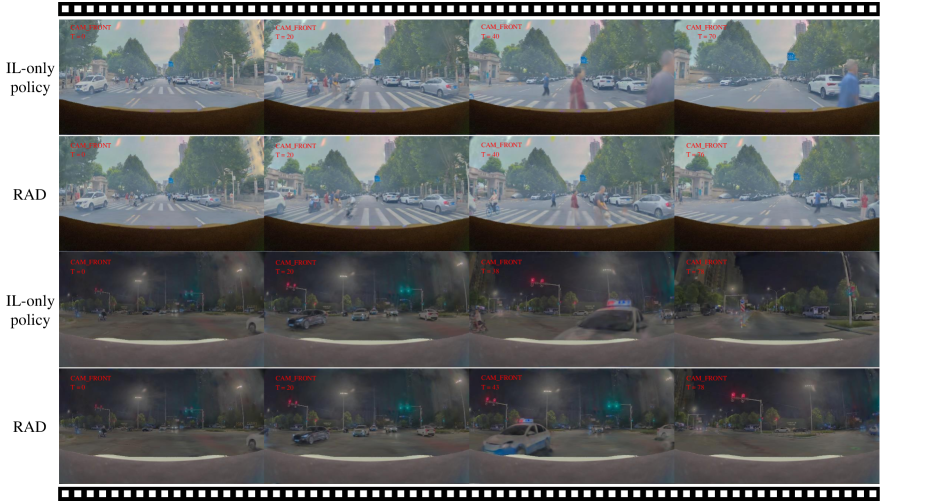
Figure 5: Closed-loop qualitative comparisons between the IL-only policy and RAD in 3DGS environments. Rows 1-2 correspond to Yield to Pedestrians. Rows 3-4 correspond to Unprotected Left-turn.

4.2 Ablation Study

To evaluate the impact of different design choices in RAD, we conduct three ablation studies. These studies examine the balance between RL and IL, the role of different reward sources, and the effect of auxiliary objectives.

RL-IL Ratio Analysis. We first analyze the effect of different RL-to-IL step mixing ratios (Tab. 1). A pure IL policy (0:1) results in the highest CR (0.229) but the lowest ADD (0.238), indicating strong trajectory consistency but poor safety. In contrast, a pure RL policy (1:0) significantly reduces CR (0.143) but increases ADD (0.345), suggesting improved safety at the cost of trajectory deviation. The best balance is achieved at a 4:1 ratio, which results in the lowest CR (0.089) while maintaining a relatively low ADD (0.257). Further increasing RL dominance (e.g., 8:1) leads to a deteriorated ADD (0.323) and higher jerk, implying reduced trajectory smoothness.

Reward Source Analysis. We analyze the influence of different reward components (Tab. 2). Policies trained with only partial reward terms (e.g., ID 1, 2, 3, 4, 5) exhibit higher collision rates (CR) compared to the full reward setup (ID 6), which achieves the lowest CR (0.089) while maintaining a stable ADD (0.257). This demonstrates that a well-balanced reward function, incorporating all reward terms, effectively enhances both safety and trajectory consistency. Among the partial reward configurations, ID 2, which omits the dynamic collision reward term, exhibits the highest CR (0.238), indicating that the absence of this term significantly impairs the model’s ability to avoid dynamic obstacles, resulting in a higher collision rate.

Auxiliary Objective Analysis. Finally, we examine the impact of auxiliary objectives (Tab. 3). Compared to the full auxiliary setup (ID 8), omitting any auxiliary objective increases CR, with a significant rise observed when all auxiliary objectives are removed. This highlights their collective role in enhancing safety. Notably, ID 1, which retains all auxiliary objectives but excludes the PPO objective, results in a CR of 0.187. This value is higher than that of ID 8, indicating that while auxiliary objectives help reduce collisions, they are most effective when combined with the PPO objective.

Our ablation studies highlight the importance of combining RL and IL, using a comprehensive reward function, and implementing structured auxiliary objectives. The optimal RL-IL ratio (4:1) and the full reward and auxiliary setups consistently yield the lowest CR while maintaining stable ADD, ensuring both safety and trajectory consistency.

4.3 Comparisons with Existing Methods

As presented in Tab. 4, we compare RAD with other end-to-end autonomous driving methods in the proposed 3DGS-based closed-loop evaluation. For fair comparisons, all the methods are trained with the same amount of human driving demonstrations. The 3DGS environments for the RL training in RAD are also based on these data. RAD achieves better performance compared to IL-based methods in most metrics. Especially in terms of CR, RAD achieves $3\times$ lower collision rate, demonstrating that RL helps the AD policy learn general collision avoidance ability.

4.4 Qualitative Comparisons

We provide qualitative comparisons between the IL-only AD policy (without reinforced post-training) and RAD, as shown in Fig. 5. The IL-only method struggles in dynamic environments, frequently failing to avoid collisions with moving obstacles or manage complex traffic situations. In contrast, RAD consistently performs well, effectively avoiding dynamic obstacles and handling challenging tasks. These results highlight the benefits of closed-loop training in the hybrid method, which enables better handling of dynamic environments. Additional visualizations are included in the Appendix (Fig. A1).

5 Limitation and Conclusion

In this work, we propose the first 3DGS-based RL framework for training end-to-end AD policy. We combine RL and IL, with RL complementing IL to model the causations and narrow the open-loop gap, and IL complementing RL in terms of human alignment. This work also has some limitations. Currently the used 3DGS environments are running in a non-reactive manner, i.e., other traffic participants do not react according to ego vehicle’s behavior but act with log replay. And the effect of 3DGS still has room for improvement, especially for rendering non-rigid pedestrians, unobserved views, and low-light scenarios. Future works will focus on solving these problems and scaling up RL to the next level.

Appendix A Appendix

A.1 Action Space Details

Here, we provide a more comprehensive explanation of the action space design. To ensure stable control and efficient learning, we define the action space over a short time horizon of 0.5 seconds. The ego vehicle’s movement is modeled using discrete displacements in both the lateral and longitudinal directions.

Lateral Displacement.

The lateral displacement, denoted as $a^{x}$, represents the vehicle’s movement in the lateral direction over the $0.5$-second horizon. We discretize this dimension into $N_{x}$ options, symmetrically distributed around zero to allow leftward and rightward movements, with an additional option to maintain the current trajectory. The set of possible lateral displacements is:

$$a^{x}\in\{d^{x}_{\text{min}},\dots,0,\dots,d^{x}_{\text{max}}\}.$$ (A1)

In our implementation, we use $N_{x}=61$, with $d^{x}_{\text{min}}=-0.75$ m, $d^{x}_{\text{max}}=0.75$ m, and intermediate values sampled uniformly.

Longitudinal Displacement.

The longitudinal displacement, denoted as $a^{y}$, represents the vehicle’s movement in the forward direction over the $0.5$-second horizon. Similar to the lateral component, we discretize this dimension into $N_{y}$ options, covering a range of forward displacements, including an option to maintain the current position:

$$a^{y}\in\{0,\dots,d^{y}_{\text{max}}\}.$$ (A2)

In our setup, we use $N_{y}=61$, with $d^{y}_{\text{max}}=15$m, and intermediate values sampled uniformly.

A.2 Implementation Details

In this section, we summarize the training settings, configurations, and hyperparameters used in our approach.

Planning Pre-Training. The action space is discretized using predefined anchors $\mathcal{A}=\{(a^{x}_{i},a^{y}_{j})\}_{i=1,j=1}^{N_{x},N_{y}}$. Each anchor corresponds to a specific steering-speed combination within the 0.5-second planning horizon. Given the ground truth vehicle position at $t=0.5\ \text{s}$ denoted as $p_{\text{gt}}=(p_{\text{gt}}^{x},p_{\text{gt}}^{y})$, we implement normalized nearest-neighbor matching over predefined anchor positions:

$$\hat{i} =\operatorname*{arg\,min}_{i}\left\|\frac{\mathbf{a}^{x}_{i}-d^{x}_{\text{min}}}{d^{x}_{\text{max}}-d^{x}_{\text{min}}}-\frac{p_{\text{gt}}^{x}-d^{x}_{\text{min}}}{d^{x}_{\text{max}}-d^{x}_{\text{min}}}\right\|_{2},$$ (A3)

$$\hat{j} =\operatorname*{arg\,min}_{j}\left\|\frac{\mathbf{a}^{y}_{j}-0}{d^{y}_{\text{max}}-0}-\frac{p_{\text{gt}}^{y}-0}{d^{y}_{\text{max}}-0}\right\|_{2}.$$

Based on the matched anchor indices $(\hat{i},\hat{j})$, we formulate the imitation learning objective as a dual focal loss [29]:

$$\mathcal{L}_{\text{IL}}=\mathcal{L}_{\text{focal}}(\pi(a^{x}\mid s),\hat{i}_{t})+\mathcal{L}_{\text{focal}}(\pi(a^{y}\mid s),\hat{j}_{t}),$$ (A4)

where $\mathcal{L}_{\text{focal}}$ is focal loss for discrete action classification, and $\pi(a^{x}\mid s)$ and $\pi(a^{y}\mid s)$ are predicted action distributions from Eq. 1.

Training configurations. We provide detailed hyperparameters for the two main stages, Planning Pre-Training and Reinforced Post-Training, in Tab. A1 and Tab. A2, respectively.

config	Planning Pre-Training
learning rate	1e-4
learning rate schedule	cosine decay
optimizer	AdamW [19, 30]
optimizer hyper-parameters	$\beta_{1}$, $\beta_{2}$, $\epsilon$ = 0.9, 0.999, 1e-8
weight decay	1e-4
batch size	512
training steps	30k
planning head dim	256

Table A1: Hyperparameters used in RAD Planning Pre-Training stage.

config	Reinforced Post-Training
learning rate	5e-6
learning rate schedule	cosine decay
optimizer	AdamW [19, 30]
optimizer hyper-parameters	$\beta_{1}$, $\beta_{2}$, $\epsilon$ = 0.9, 0.999, 1e-8
weight decay	1e-4
RL worker number	32
RL batch size	32
IL batch size	128
GAE parameter	$\gamma=0.9$, $\lambda=0.95$
clipping thresholds	$\epsilon_{x}=0.1$, $\epsilon_{y}=0.2$
deviation threshold	$d_{\text{max}}=2.0m$, $\psi_{\text{max}}=40^{\circ}$
planning head dim	256
value function dim	256

Table A2: Hyperparameters used in RAD Reinforced Post-Training stage.

A.3 Metric Details

We evaluate the performance of the autonomous driving policy using eight key metrics.

Dynamic Collision Ratio (DCR). DCR quantifies the frequency of collisions with dynamic obstacles. It is defined as:

$$DCR=\frac{N_{dc}}{N_{total}},$$ (A5)

where $N_{dc}$ is the number of clips in which collisions with dynamic obstacles occur, and $N_{total}$ is the total number of clips.

Static Collision Ratio (SCR). SCR measures the frequency of collisions with static obstacles and is defined as:

$$SCR=\frac{N_{sc}}{N_{total}},$$ (A6)

where $N_{sc}$ is the number of clips with static obstacle collisions.

Collision Ratio (CR). CR represents the total collision frequency, given by:

$$CR=DCR+SCR.$$ (A7)

Positional Deviation Ratio (PDR). PDR evaluates the ego vehicle’s adherence to the expert trajectory in terms of position. It is defined as:

$$PDR=\frac{N_{pd}}{N_{total}},$$ (A8)

where $N_{pd}$ is the number of clips in which the positional deviation exceeds a predefined threshold.

Heading Deviation Ratio (HDR). HDR assesses orientation accuracy by computing the proportion of clips where heading deviations surpass a predefined threshold:

$$HDR=\frac{N_{hd}}{N_{total}},$$ (A9)

where $N_{hd}$ is the number of clips where the heading deviation exceeds the threshold.

Deviation Ratio (DR). captures the overall deviation from the expert trajectory, given by:

$$DR=PDR+HDR.$$ (A10)

Average Deviation Distance (ADD). ADD quantifies the mean closest distance between the ego vehicle and the expert trajectory during time steps when no collisions or deviations occur. It is defined as:

$$ADD=\frac{1}{T_{safe}}\sum_{t=1}^{T_{safe}}d_{min}(t),$$ (A11)

where $T_{safe}$ represents the total number of time steps in which the ego vehicle operates without collisions or deviations, and $d_{min}(t)$ denotes the minimum distance between the ego vehicle and the expert trajectory at time step $t$.

Finally, Longitudinal Jerk (Long. Jerk) and Lateral Jerk (Lat. Jerk) quantify the smoothness of vehicle motion by measuring acceleration changes. Longitudinal jerk is defined as:

$$J_{long}=\frac{d^{2}v_{long}}{dt^{2}},$$ (A12)

where $v_{long}$ represents the longitudinal velocity. Similarly, lateral jerk is defined as:

$$J_{lat}=\frac{d^{2}v_{lat}}{dt^{2}},$$ (A13)

where $v_{lat}$ is the lateral velocity. These metrics collectively capture abrupt changes in acceleration and steering, providing a comprehensive measure of passenger comfort and driving stability.

A.4 More Qualitative Results

This section presents additional qualitative comparisons across various driving scenarios, including detours, crawling in dense traffic, traffic congestion, and U-turn maneuvers. The results highlight the effectiveness of our approach in generating smoother trajectories, enhancing collision avoidance, and improving adaptability in complex environments.

Figure A1: More Qualitative Results. Comparison between the IL-only policy and RAD in various driving scenarios: Detour (Rows 1-2), Crawl in Dense Traffic (Rows 3-4), Traffic Congestion (Rows 5-6), and U-turn(Rows 7-8).

References

- Chen et al. [2021] Dian Chen, Vladlen Koltun, and Philipp Krähenbühl. Learning to drive from a world on rails. In ICCV, 2021.
- Chen et al. [2024a] Shaoyu Chen, Bo Jiang, Hao Gao, Bencheng Liao, Qing Xu, Qian Zhang, Chang Huang, Wenyu Liu, and Xinggang Wang. Vadv2: End-to-end vectorized autonomous driving via probabilistic planning. arXiv preprint arXiv:2402.13243, 2024a.
- Chen et al. [2024b] Zhili Chen, Maosheng Ye, Shuangjie Xu, Tongyi Cao, and Qifeng Chen. Ppad: Iterative interactions of prediction and planning for end-to-end autonomous driving. In ECCV, 2024b.
- DeepSeek-AI [2025] DeepSeek-AI. Deepseek-r1: Incentivizing reasoning capability in llms via reinforcement learning, 2025.
- Dosovitskiy [2020] Alexey Dosovitskiy. An image is worth 16x16 words: Transformers for image recognition at scale. arXiv preprint arXiv:2010.11929, 2020.
- Dosovitskiy et al. [2017] Alexey Dosovitskiy, German Ros, Felipe Codevilla, Antonio Lopez, and Vladlen Koltun. Carla: An open urban driving simulator. In Conference on robot learning, pages 1–16. PMLR, 2017.
- Games [1998] Epic Games. Unreal engine. https://www.unrealengine.com/, 1998.
- Geirhos et al. [2020] Robert Geirhos, Jörn-Henrik Jacobsen, Claudio Michaelis, Richard Zemel, Wieland Brendel, Matthias Bethge, and Felix A Wichmann. Shortcut learning in deep neural networks. Nature Machine Intelligence, 2020.
- Gu et al. [2024] Xunjiang Gu, Guanyu Song, Igor Gilitschenski, Marco Pavone, and Boris Ivanovic. Producing and leveraging online map uncertainty in trajectory prediction. In CVPR, 2024.
- He et al. [2016] Kaiming He, Xiangyu Zhang, Shaoqing Ren, and Jian Sun. Deep residual learning for image recognition. In Proceedings of the IEEE conference on computer vision and pattern recognition, 2016.
- Hu et al. [2022] Yihan Hu, Jiazhi Yang, Li Chen, Keyu Li, Chonghao Sima, Xizhou Zhu, Siqi Chai, Senyao Du, Tianwei Lin, Wenhai Wang, et al. Planning-oriented autonomous driving. CVPR2023, 2022.
- Hu et al. [2023] Yihan Hu, Jiazhi Yang, Li Chen, Keyu Li, Chonghao Sima, Xizhou Zhu, Siqi Chai, Senyao Du, Tianwei Lin, Wenhai Wang, et al. Planning-oriented autonomous driving. In CVPR, 2023.
- Hu et al. [2024] Yihan Hu, Siqi Chai, Zhening Yang, Jingyu Qian, Kun Li, Wenxin Shao, Haichao Zhang, Wei Xu, and Qiang Liu. Solving motion planning tasks with a scalable generative model. In ECCV, 2024.
- Intuition [2023] Applied Intuition. Carsim. https://www.carsim.com/, 2023.
- Jiang et al. [2022] Bo Jiang, Shaoyu Chen, Xinggang Wang, Bencheng Liao, Tianheng Cheng, Jiajie Chen, Helong Zhou, Qian Zhang, Wenyu Liu, and Chang Huang. Perceive, interact, predict: Learning dynamic and static clues for end-to-end motion prediction. arXiv preprint arXiv:2212.02181, 2022.
- Jiang et al. [2023a] Bo Jiang, Shaoyu Chen, Qing Xu, Bencheng Liao, Jiajie Chen, Helong Zhou, Qian Zhang, Wenyu Liu, Chang Huang, and Xinggang Wang. Vad: Vectorized scene representation for efficient autonomous driving. In ICCV, 2023a.
- Jiang et al. [2023b] Bo Jiang, Shaoyu Chen, Qing Xu, Bencheng Liao, Jiajie Chen, Helong Zhou, Qian Zhang, Wenyu Liu, Chang Huang, and Xinggang Wang. Vad: Vectorized scene representation for efficient autonomous driving. ICCV, 2023b.
- Kerbl et al. [2023] Bernhard Kerbl, Georgios Kopanas, Thomas Leimkühler, and George Drettakis. 3d gaussian splatting for real-time radiance field rendering. ACM Trans. Graph., 42(4):139–1, 2023.
- Kingma and Ba [2014] Diederik P Kingma and Jimmy Ba. Adam: A method for stochastic optimization. arXiv preprint arXiv:1412.6980, 2014.
- Li et al. [2024a] Yingyan Li, Lue Fan, Jiawei He, Yuqi Wang, Yuntao Chen, Zhaoxiang Zhang, and Tieniu Tan. Enhancing end-to-end autonomous driving with latent world model. arXiv preprint arXiv:2406.08481, 2024a.
- Li et al. [2022] Zhiqi Li, Wenhai Wang, Hongyang Li, Enze Xie, Chonghao Sima, Tong Lu, Qiao Yu, and Jifeng Dai. Bevformer: Learning bird’s-eye-view representation from multi-camera images via spatiotemporal transformers. arXiv preprint arXiv:2203.17270, 2022.
- Li et al. [2024b] Zhenxin Li, Kailin Li, Shihao Wang, Shiyi Lan, Zhiding Yu, Yishen Ji, Zhiqi Li, Ziyue Zhu, Jan Kautz, Zuxuan Wu, et al. Hydra-mdp: End-to-end multimodal planning with multi-target hydra-distillation. arXiv preprint arXiv:2406.06978, 2024b.
- Li et al. [2024c] Zhiqi Li, Zhiding Yu, Shiyi Lan, Jiahan Li, Jan Kautz, Tong Lu, and Jose M Alvarez. Is ego status all you need for open-loop end-to-end autonomous driving? In CVPR, 2024c.
- Li et al. [2024d] Zhiqi Li, Zhiding Yu, Shiyi Lan, Jiahan Li, Jan Kautz, Tong Lu, and Jose M Alvarez. Is ego status all you need for open-loop end-to-end autonomous driving? In CVPR, 2024d.
- Liao et al. [2022] Bencheng Liao, Shaoyu Chen, Xinggang Wang, Tianheng Cheng, Qian Zhang, Wenyu Liu, and Chang Huang. Maptr: Structured modeling and learning for online vectorized hd map construction. arXiv preprint arXiv:2208.14437, 2022.
- Liao et al. [2023a] Bencheng Liao, Shaoyu Chen, Bo Jiang, Tianheng Cheng, Qian Zhang, Wenyu Liu, Chang Huang, and Xinggang Wang. Lane graph as path: Continuity-preserving path-wise modeling for online lane graph construction. arXiv preprint arXiv:2303.08815, 2023a.
- Liao et al. [2023b] Bencheng Liao, Shaoyu Chen, Yunchi Zhang, Bo Jiang, Qian Zhang, Wenyu Liu, Chang Huang, and Xinggang Wang. Maptrv2: An end-to-end framework for online vectorized hd map construction. arXiv preprint arXiv:2308.05736, 2023b.
- Liao et al. [2024] Bencheng Liao, Shaoyu Chen, Haoran Yin, Bo Jiang, Cheng Wang, Sixu Yan, Xinbang Zhang, Xiangyu Li, Ying Zhang, Qian Zhang, and Xinggang Wang. Diffusiondrive: Truncated diffusion model for end-to-end autonomous driving. arXiv preprint arXiv:2411.15139, 2024.
- Lin et al. [2017] Tsung-Yi Lin, Priya Goyal, Ross Girshick, Kaiming He, and Piotr Dollár. Focal loss for dense object detection. In ICCV, 2017.
- Loshchilov and Hutter [2019] Ilya Loshchilov and Frank Hutter. Decoupled weight decay regularization. In ICLR, 2019.
- Lu et al. [2023] Yiren Lu, Justin Fu, George Tucker, Xinlei Pan, Eli Bronstein, Rebecca Roelofs, Benjamin Sapp, Brandyn White, Aleksandra Faust, Shimon Whiteson, Dragomir Anguelov, and Sergey Levine. Imitation is not enough: Robustifying imitation with reinforcement learning for challenging driving scenarios. In IROS, 2023.
- OpenAI [2024] OpenAI. Openai o1. https://openai.com/o1/, 2024.
- Prakash et al. [2021] Aditya Prakash, Kashyap Chitta, and Andreas Geiger. Multi-modal fusion transformer for end-to-end autonomous driving. 2021.
- Schulman et al. [2015] John Schulman, Philipp Moritz, Sergey Levine, Michael Jordan, and Pieter Abbeel. High-dimensional continuous control using generalized advantage estimation. arXiv preprint arXiv:1506.02438, 2015.
- Schulman et al. [2017] John Schulman, Filip Wolski, Prafulla Dhariwal, Alec Radford, and Oleg Klimov. Proximal policy optimization algorithms. arXiv preprint arXiv:1707.06347, 2017.
- Silver et al. [2016] David Silver, Aja Huang, Chris J Maddison, Arthur Guez, Laurent Sifre, George Van Den Driessche, Julian Schrittwieser, Ioannis Antonoglou, Veda Panneershelvam, Marc Lanctot, et al. Mastering the game of go with deep neural networks and tree search. nature, 2016.
- Silver et al. [2017] David Silver, Julian Schrittwieser, Karen Simonyan, Ioannis Antonoglou, Aja Huang, Arthur Guez, Thomas Hubert, Lucas Baker, Matthew Lai, Adrian Bolton, Yutian Chen, Timothy P. Lillicrap, Fan Hui, Laurent Sifre, George van den Driessche, Thore Graepel, and Demis Hassabis. Mastering the game of go without human knowledge. Nat., 2017.
- Sun et al. [2024] Wenchao Sun, Xuewu Lin, Yining Shi, Chuang Zhang, Haoran Wu, and Sifa Zheng. Sparsedrive: End-to-end autonomous driving via sparse scene representation. arXiv preprint arXiv:2405.19620, 2024.
- Technologies [2005] Unity Technologies. Unity. https://https://unity.com/, 2005.
- Tonderski et al. [2023] Adam Tonderski, Carl Lindstrom, Georg Hess, William Ljungbergh, Lennart Svensson, and Christoffer Petersson. Neurad: Neural rendering for autonomous driving. 2024 IEEE/CVF Conference on Computer Vision and Pattern Recognition (CVPR), pages 14895–14904, 2023.
- Toromanoff et al. [2020] Marin Toromanoff, Emilie Wirbel, and Fabien Moutarde. End-to-end model-free reinforcement learning for urban driving using implicit affordances. In CVPR, 2020.
- Wang et al. [2024] Yuqi Wang, Jiawei He, Lue Fan, Hongxin Li, Yuntao Chen, and Zhaoxiang Zhang. Driving into the future: Multiview visual forecasting and planning with world model for autonomous driving. In CVPR, 2024.
- Weng et al. [2024] Xinshuo Weng, Boris Ivanovic, Yan Wang, Yue Wang, and Marco Pavone. Para-drive: Parallelized architecture for real-time autonomous driving. In CVPR, 2024.
- Wu et al. [2023] Zirui Wu, Tianyu Liu, Liyi Luo, Zhide Zhong, Jianteng Chen, Hongmin Xiao, Chao Hou, Haozhe Lou, Yuan-Hao Chen, Runyi Yang, Yuxin Huang, Xiaoyu Ye, Zike Yan, Yongliang Shi, Yiyi Liao, and Hao Zhao. Mars: An instance-aware, modular and realistic simulator for autonomous driving. ArXiv, 2023.
- Yan et al. [2024] Yunzhi Yan, Haotong Lin, Chenxu Zhou, Weijie Wang, Haiyang Sun, Kun Zhan, Xianpeng Lang, Xiaowei Zhou, and Sida Peng. Street gaussians: Modeling dynamic urban scenes with gaussian splatting. In European Conference on Computer Vision, 2024.
- Yang et al. [2023] Ze Yang, Yun Chen, Jingkang Wang, Sivabalan Manivasagam, Wei-Chiu Ma, Anqi Joyce Yang, and Raquel Urtasun. Unisim: A neural closed-loop sensor simulator. 2023 IEEE/CVF Conference on Computer Vision and Pattern Recognition (CVPR), 2023.
- Zhai et al. [2023] Jiang-Tian Zhai, Ze Feng, Jihao Du, Yongqiang Mao, Jiang-Jiang Liu, Zichang Tan, Yifu Zhang, Xiaoqing Ye, and Jingdong Wang. Rethinking the open-loop evaluation of end-to-end autonomous driving in nuscenes. arXiv preprint arXiv:2305.10430, 2023.
- Zhang et al. [2021] Zhejun Zhang, Alexander Liniger, Dengxin Dai, Fisher Yu, and Luc Van Gool. End-to-end urban driving by imitating a reinforcement learning coach. 2021.
- Zheng et al. [2024] Wenzhao Zheng, Ruiqi Song, Xianda Guo, Chenming Zhang, and Long Chen. Genad: Generative end-to-end autonomous driving. In ECCV, 2024.
- Zhou et al. [2024] Hongyu Zhou, Longzhong Lin, Jiabao Wang, Yichong Lu, Dongfeng Bai, Bingbing Liu, Yue Wang, Andreas Geiger, and Yiyi Liao. Hugsim: A real-time, photo-realistic and closed-loop simulator for autonomous driving. arXiv preprint arXiv:2412.01718, 2024.
- Zhou et al. [2023] Xiaoyu Zhou, Zhiwei Lin, Xiaojun Shan, Yongtao Wang, Deqing Sun, and Ming-Hsuan Yang. Drivinggaussian: Composite gaussian splatting for surrounding dynamic autonomous driving scenes. 2024 IEEE/CVF Conference on Computer Vision and Pattern Recognition (CVPR), pages 21634–21643, 2023.