Stochastic Schrödinger equation for homodyne measurements of strongly correlated systems

Abstract

We derive a stochastic Schrödinger equation that describes the homodyne measurement record of a strongly interacting atomic system. We derive this equation for a general system, where we use the rotating wave approximation in the linear atom-light interaction part, and the resulting equation is expressed in terms of the atomic operators only. Weak measurements are theoretically described in terms of positive operator-valued measures. Among different weak measurement schemes, several earlier references studied the Gaussian quantum continuous measurement in detail. Here we consider a homodyne measurement setup. We then demonstrate that the derived equation for this setup in the appropriate limit is the same as the one obtained while performing a Gaussian quantum continuous measurement.

• Keywords: ultracold dynamics, optical and laser physics, homodyne measurement.

1 Introduction

When a physical property of a quantum state $|\Psi\rangle$ is measured, one describes the result traditionally in terms of a projective measurement that causes the state to collapse. We associate an observable $\hat{\Lambda}$, which is generally represented as a Hermitian matrix, to the measured physical property, e.g., momentum. It is then possible to write $\hat{\Lambda}=\sum_{\lambda}\lambda\hat{\Pi}_{\lambda}$, where $\{\lambda\}$ are the real eigenvalues of $\hat{\Lambda}$ and $\hat{\Pi}_{\lambda}=|\lambda\rangle\langle\lambda|$ are rank-1 projectors. If the projective measurement produces a result $\lambda$, the quantum state must have been projected by $\hat{\Pi}_{\lambda}$ into the eigenstate $|\lambda\rangle$. For instance, the time of flight measurement that one performs to probe different phases of interacting atomic Hamiltonians in optical lattices are analyzed within this projective measurement paradigm [1, 2].

We instead focus on a more realistic description of an experimental setup, where the system of interest is not directly measured. Rather, the system interacts with a second quantum system (called the meter or the apparatus), and the meter is later measured projectively. Unlike in a projective measurement, after such generalized measurement, one obtains a state that is peaked about an eigenstate $|\lambda\rangle$ with a certain width. A large width means more uncertainty in obtaining the corresponding eigenvalue $\lambda$. A generalized measurement, where one manages to extract only infinitesimal information about the system, is referred to as a weak measurement. Recently, this concept of weak measurement has been invoked in several optics experiments. For instance, an experiment depicting the spin Hall effect of light treats the phenomenon as a weak measurement of the spin projection of the photons [3]. Weak measurement schemes were also employed to detect the Goos-Hänchen and Imbert-Fedorov shifts in partial reflection [4, 5, 6].

One need not explicitly include the meter in the description of a weak measurement. It is possible to describe the measurement scheme by the action of a set of generalized measurement operators $\{\hat{M}_{r}\}$ on the system, where $\{r\}$ denotes the corresponding measurement outcomes [7, 8, 9, 10, 11]. Note that, by $\{r\}$, we denote the real eigenvalues of an ancillary observable. After the measurement process, if one obtains a result $r$, the state of the system is given by $\hat{M}_{r}|\Psi\rangle/\mathcal{P}_{r},$ where $\mathcal{P}_{r}$ is the probability of getting the particular result $r$. This probability $\mathcal{P}_{r}$ is defined in terms of the probability operators or effects $\hat{E}_{r}=\hat{M}_{r}^{\dagger}\hat{M}_{r}$ as $\mathcal{P}_{r}=\langle\Psi|\hat{E}_{r}|\Psi\rangle.$ Since $\sum_{r}\mathcal{P}_{r}=1$, one must have $\sum_{r}\hat{E}_{r}=\mathbb{1}$. Compare this with the resolution of identity $\sum_{\lambda}\hat{\Pi}_{\lambda}=\mathbb{1}$ for projective measurements. The set of all these effects $\{\hat{E}_{r}:r\}$ is referred to as a positive operator-valued measure (POVM).

The generalized measurement operator given by

$$\hat{M}(\alpha)=\left(\frac{4\mathcal{K}\mathrm{d}t}{\pi}\right)^{1/4}\int_{-\infty}^{+\infty}e^{-2\mathcal{K}\mathrm{d}t\left(x-\alpha\right)^{2}}\left|x\right\rangle\left\langle x\right|\mathrm{d}x$$ (1)

corresponds to the Gaussian quantum continuous measurement of the Hermitian operator $\hat{X}$ at a sequence of intervals of length $\mathrm{d}t$ and with measurement strength $\mathcal{K}$ [7, 8]. The Hermitian operator $\hat{X}$ has a continuous spectrum of eigenvalues $x$ and orthonormal eigenstates $|x\rangle$ with the property $\langle x|x^{\prime}\rangle=\delta\left(x-x^{\prime}\right)$. The continuous indices $\alpha$ are the eigenvalues of an ancillary observable and are the possible measurement outcomes. They are not, however, the eigenvalues of either $\hat{M}(\alpha)$ or $\hat{X}$. At this point, however, it is not immediately clear how the generalized measurement operators are connected to the real experimental setups, e.g., the setup considered in Ref. [12].

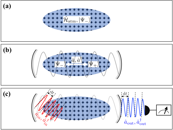
Figure 1: Studying strongly correlated systems inside an optical cavity. In the panel (a) of the schematic diagram above, we show the strongly correlated Hamiltonian $\hat{H}_{\text{atm}}$ realized by trapping ultracold atoms in an optical lattice. The ground state of this Hamiltonian $|\Psi_{-}\rangle$ has interesting properties that one would like to explore. In panel (b), we depict the strongly correlated atomic system inside a single mode optical cavity. The annihilation (creation) operator for this mode is $\hat{a}(\hat{a}^{\dagger})$. Although the cavity mode photons couple the ground state $|\Psi_{-}\rangle$ to the excited state $|\Psi_{+}\rangle$, it is possible to adiabatically eliminate the excited state and obtain an effective dispersive atom-light Hamiltonian (9). In panel (c), we show the external driving laser – input field $(\hat{a}_{\mathrm{in}},\hat{a}_{\mathrm{in}}^{\dagger})$ – in red [13]. This then gives rise to the output field $(\hat{a}_{\mathrm{out}},\hat{a}_{\mathrm{out}}^{\dagger})$. The input field populates the cavity, and the output field – which is entangled with the strongly correlated system inside the cavity – is finally detected. The output photons are detected with a homodyne setup, see Fig. 2. In fact, this set up detects the linear combinations of the local oscillator and output mode. We show that in an appropriate limit the measurement record is appropriately described by an SSE (62) in terms of only the atomic degrees of freedom, which is equivalent to the SSE that is obtained when one performs a Gaussian continuous quantum measurement of an atomic observable $\hat{\mathcal{M}}_{0}$ on $\hat{\mathcal{H}}_{\text{atm}}$.

In this paper, we introduce a scheme to study the properties of a correlated many-body system in Fig. 1. As shown in Fig. 1(b), the system of interest – for example, strongly interacting ultracold atoms in an optical trap described by the Hamiltonian $\hat{\mathcal{H}}_{\text{atm}}$ – interacts further with the cavity mode photons. The cavity is driven by an external laser. The small time segments of length $\mathrm{d}t$ of the input light are treated as single modes, which are also considered to be in the coherent state $\left|\alpha\right\rangle$ right before the driving laser enters the cavity [14], see Fig. 1(c). After interaction, however, the output field is entangled with the interacting atomic system and it no longer factorizes. Thus, we vicariously analyse the properties of $\hat{\mathcal{H}}_{\text{atm}}$ by detecting the output field $(\hat{a}_{\mathrm{out}},\hat{a}_{\mathrm{out}}^{\dagger})$ using a homodyne setup. In this setup (see Fig. 2), after mixing the output light further with another beam of coherent light of high intensity (a local oscillator), we perform projective measurements on the light. Since this measurement procedure does not destroy the quantum entanglement of the system of interest, one can keep probing the atomic system $\hat{\mathcal{H}}_{\text{atm}}$ for a prolonged period of time.

• 

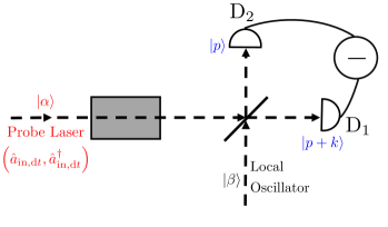
Figure 2: In this experimental setup, the gray shaded box represents the cavity, where the strongly interacting Hamiltonian is engineered using cold atoms in optical lattices. The slanted straight line is the 50:50 beam splitter. The two detectors are marked as $\textrm{D}_{1}$ and $\textrm{D}_{2}$. This figure has been reused with modifications from Ref. [12].

Here, we derive a stochastic Schrödinger equation (SSE) that describes how the atomic state of Figs. 1 and 2 evolves in time. In this SSE, the homodyne measurement process gives rise to a term proportional to a Wiener process. We derive an SSE purely in terms of the atomic degrees of freedom. We demonstrate that, in the strong local oscillator and weak driving laser limit, the derived SSE is analogous to the one obtained by considering the action of the generalized measurement operator (1) corresponding to a Gaussian quantum continuous measurement on the atomic part of the total wavefunction.

Before describing our scheme and the resulting SSE, we summarize the related discussion in earlier references in this paragraph [7, 8, 9, 10, 11]. Instead of considering a homodyne measurement, one generally starts by describing the measurement of the output light with a photon counting setup. This leads to an SSE that contains terms proportional to a Poisson process. In that equation, the output photons are directly detected as quantum jumps. To go from a photon counting to a homodyne measurement, one then introduces a local oscillator that interferes with the output light field. This results in an SSE that involves a continuous Wiener process instead of a discrete Poisson process. To obtain this, one uses the well known result: in the limit of quantum jumps detected in an infinitesimal time interval being quite large, the Poisson distribution becomes the Gaussian distribution.

Our approach to the SSE here is similar to the one provided in Ref. [14]. We model all the processes – which include the effects of the beam splitters – in the infinitesimal time interval right before the photons are detected by the detectors $\textrm{D}_{1}$ and $\textrm{D}_{2}$ as unitary matrices acting on the quantum state. The resulting SSE regards the output photon detections after interference with a local oscillator as projective measurements. Note that the SSE derived here is expressed exclusively in terms of the atomic operators unlike the one in [14]. Unlike in [14], we recover an SSE having the canonical form expected for a Gaussian quantum continuous measurement (e.g., the SSE considered in Ref. [12]) in the appropriate limit.

In this paper, we start with the full atom-light Hamiltonian in a Fabry-Pérot cavity in Sec. 2. This Hamiltonian is depicted in Fig. 1(b). The cavity – which is driven by an external laser (the input field), see Fig. 1(c) – gives rise to a particular spatial mode function, which then leads to a specific measurement operator. The fast relaxation of the cavity permits us to express the cavity field in terms of the input field and the system observables. After adiabatically eliminating the excited atomic states and displacing the light mode by its coherent expectation value, we arrive at an effective Hamiltonian that manifests the linear coupling between the Hermitian measurement operator and the driving (input) light mode.

In Sec. 3, we start from the density matrix (containing the atomic part, the probe laser, and the local oscillator) conditioned upon the detection of $p+k$ photons at the detector $\textrm{D}_{1}$ and $p$ photons at the detector $\textrm{D}_{2}$, where $p$ is an arbitrary positive integer. The output signal that is entangled with the strongly interacting atomic system inside the cavity mixes with the light mode of a local oscillator, which is assumed to be in the coherent state $\left|\beta\right\rangle$ during a small time interval $\mathrm{d}t$. We show that the measurement record of the photon number difference $k$ in the strong local oscillator limit with $\beta^{2}=\mathcal{O}(1/\mathrm{d}t)\gg 1$ has an additive Wiener noise. Using this information in the conditional (a-posteriori) density matrix, we demonstrate that the resultant SSE is the same as the one obtained for a Gaussian quantum continuous measurement.

Finally in Sec. 4, we numerically study the properties of the derived SSE. In particular, we show that one can detect the signatures of the superfluid to Mott-insulator phase transition of the Bose-Hubbard model in the time dependent dynamics of the expectation values of the measurement operators in the weak measurement regime. Similar to Ref. [12], we first consider the measurement of the sum over coherences $\hat{\mathcal{M}}_{\mathrm{coh}}$ and then the sum of the number of atoms in the even sites $\hat{\mathcal{M}}_{\mathrm{pop}}$. We also show the examples of quantum trajectories in the quantum Zeno regime [19, 20, 21, 22] for large measurement strengths.

2 Derivation of the Effective Hamiltonian

We start with the atom-light Hamiltonian of Fig. 1(b), where the atomic ground and excited states are coupled via the cavity mode. Assuming that the detuning between the laser frequency and the frequency of the atomic excitation is large, we adiabatically eliminate the atomic excited state. This leads to the dispersive atom-light interacting Hamiltonian of the cavity.

In the dipole approximation, the full atom-light Hamiltonian is given by

$$\hat{\mathcal{H}}=\hat{\mathcal{H}}_{A}+\hat{\mathcal{H}}_{\text{atm}}+\hat{\mathcal{H}}_{a}+g\hat{a}\int\hat{\Psi}_{+}^{\dagger}(x)f_{a}(x,\omega_{\text{L}})\hat{\Psi}_{-}(x)\;\mathrm{d}x\\ +g\hat{a}^{\dagger}\int\hat{\Psi}_{-}^{\dagger}(x)f_{a}(x,\omega_{\text{L}})\hat{\Psi}_{+}(x)\;\mathrm{d}x,$$ (2)

where $\hat{\Psi}_{+(-)}$ is the bosonic field operator for the excited (ground) state of the atoms and we have neglected the fast-rotating terms. The probe field, which we assume to be in resonance with the cavity, has frequency $\omega_{\text{L}}$ and $g$ is the coupling strength [1]. Moreover, we have $\hat{\mathcal{H}}_{A}=\omega_{eg}\int\text{d}x\;\hat{\Psi}_{+}^{\dagger}(x)\hat{\Psi}_{+}(x)$ corresponding to the atomic excited state and $\hat{\mathcal{H}}_{a}=\omega_{\text{L}}\hat{a}^{\dagger}\hat{a}$ corresponding to the free Hamiltonian of the cavity light field with the spatial mode function $f_{a}(x,\omega_{\text{L}})$. For a concrete example, where $\hat{\mathcal{H}}_{\text{atm}}$ is the same as the Bose-Hubbard Hamiltonian, see Ref. [15].

We introduce the fields that vary slowly with time

$$\hat{\widetilde{a}}=e^{i\omega_{\text{L}}t}\hat{a},\quad\hat{\widetilde{\Psi}}_{+}=\hat{\Psi}_{+}e^{i\omega_{eg}t},$$ (3)

where we have included the free evolution of the excited state and the light field into the new field operators (in the Schrödinger picture itself). Recall that in the Heisenberg picture an observable satisfies the equation

$$\frac{\mathrm{d}}{\mathrm{d}t}\hat{A}_{H}(t)=i\left[\hat{\mathcal{H}}_{H},\hat{A}_{H}(t)\right]+\left(\frac{\partial\hat{A}_{S}}{\partial t}\right)_{H},$$ (4)

where the subscripts $H$ and $S$ denote Heisenberg and Schrödinger picture, respectively. Using this, we find that the new fields have the following equations of motion:

$$\frac{\mathrm{d}\hat{\widetilde{a}}}{\mathrm{d}t}=-ig\int\hat{\widetilde{\Psi}}_{-}^{\dagger}(x)f_{a}(x,\omega_{L})\hat{\widetilde{\Psi}}_{+}(x)e^{i\Delta t}\mathrm{d}x,$$ (5a)

$$\frac{\mathrm{d}}{\mathrm{d}t}\hat{\widetilde{\Psi}}_{+}(x)=-ig\hat{\widetilde{a}}\hat{\widetilde{\Psi}}_{-}(x)f_{a}(x,\omega_{L})e^{-i\Delta t},$$ (5b)

where $\Delta=\omega_{L}-\omega_{eg}$ is the detuning of the probe from the atomic transition. We assume $\Delta\gg g,$ and initially all the atoms are in their ground state. In that case, noting that the time dependence of Eq. (5b) is dominated by the rotating term, we obtain

$$\hat{\widetilde{\Psi}}_{+}(x)=\frac{g}{\Delta}\hat{\widetilde{a}}\hat{\widetilde{\Psi}}_{-}(x)f_{a}(x,\omega_{L})e^{-i\Delta t},$$ (6)

which allows us to adiabatically eliminate the excited atomic state and write

$$\frac{\mathrm{d}\hat{\widetilde{a}}}{\mathrm{d}t}=-\frac{ig^{2}}{\Delta}\hat{\widetilde{a}}\int|f_{a}(x,\omega_{L})|^{2}\hat{\widetilde{\Psi}}_{-}^{\dagger}(x)\hat{\widetilde{\Psi}}_{-}(x)\;\mathrm{d}x.$$ (7)

With the help of Eq. (4), one notices that the effective Hamiltonian

$$\hat{\widetilde{\mathcal{H}}}=\hat{\mathcal{H}}_{\text{atm}}+\frac{g^{2}}{\Delta}\int|f_{a}(x,\omega_{L})|^{2}\hat{\widetilde{\Psi}}^{\dagger}(x)\hat{\widetilde{\Psi}}(x)\hat{\widetilde{a}}^{\dagger}\hat{\widetilde{a}}\;\mathrm{d}x$$ (8)

gives rise to the equation of motion (7), where the subscript for the atomic field operator has now been dropped. This then gives the following effective Hamiltonian in terms of the original field operators:

$$\hat{\mathcal{H}}=\hat{\mathcal{H}}_{\text{atm}}+\hat{\mathcal{H}}_{a}+\frac{g^{2}}{\Delta}\int|f_{a}(x,\omega_{L})|^{2}\hat{\Psi}^{\dagger}(x)\hat{\Psi}(x)\hat{a}^{\dagger}\hat{a}\;\mathrm{d}x.$$ (9)

The localized (at the minima of the optical lattice potential) Wannier functions form a complete set for the first band of the atomic system. We now expand the field operators in terms of these functions as

$$\hat{\Psi}(x)=\sum_{j}\hat{b}_{j}w_{j}(x).$$ (10)

The creation operators $\hat{b}^{\dagger}_{i}$ creates a boson at the lattice site $i$. The relevant matrix determining the spatial influence of the measurement is obtained by expressing the integral in Hamiltonian (9) in terms of these Wannier functions. The resulting Hamiltonian reads

$$\hat{\mathcal{H}}=\hat{\mathcal{H}}_{\text{atm}}+\hat{\mathcal{H}}_{a}+\sum_{j,k}M_{jk}\hat{b}_{j}^{\dagger}\hat{b}_{k}\hat{a}^{\dagger}\hat{a},$$ (11)

with

$$M_{jk}=\frac{g^{2}}{\Delta}\int|f_{a}(x,\omega_{L})|^{2}w_{j}^{*}(x)w_{k}(x)\mathrm{d}x.$$ (12)

The cavity mode $(\hat{a},\hat{a}^{\dagger})$ in the Hamiltonian (11) is populated by an external laser as depicted in Fig. 1(c). Using the input-output theory to model this system [13], we obtain the Heisenberg-Langevin equation

$$\dot{\hat{a}}=-i\omega_{L}\hat{a}-i\sum_{jk}M_{jk}\hat{b}^{\dagger}_{j}\hat{b}_{k}\hat{a}-\kappa\hat{a}+\eta+\sqrt{2\kappa}\hat{a}_{\mathrm{in}},$$ (13)

with $\hat{a}_{\mathrm{in}}$ being the annihilation operator corresponding to the input field, $2\kappa$ the cavity mode decay rate, and $\eta$ the pump power [8]. We displace $\hat{a}$ by its coherent expectation value

$$\hat{a}\to\mathcal{A}+\hat{a}$$ (14)

such that we have

$$\dot{\hat{a}}+\dot{\mathcal{A}}=-i\omega_{L}\mathcal{A}-i\omega_{L}\hat{a}-i\sum_{jk}M_{jk}\hat{b}^{\dagger}_{j}\hat{b}_{k}\mathcal{A}\\ -i\sum_{jk}M_{jk}\hat{b}^{\dagger}_{j}\hat{b}_{k}\hat{a}-\kappa\mathcal{A}-\kappa\hat{a}+\eta+\sqrt{2\kappa}\hat{a}_{\mathrm{in}}.$$ (15)

We choose $\mathcal{A}=\mathcal{A}_{0}$ to be the solution of

$$\dot{\mathcal{A}}=-i\omega_{L}\mathcal{A}-\kappa\mathcal{A}+\eta,$$ (16)

such that $\hat{a}$ obeys

$$\dot{\hat{a}}=-i\omega_{L}\hat{a}-i\mathcal{A}_{0}\sum_{jk}M_{jk}\hat{b}^{\dagger}_{j}\hat{b}_{k}-\kappa\hat{a}+\sqrt{2\kappa}\hat{a}_{\mathrm{in}},$$ (17)

where we have neglected the term coupling the quantum operators directly compared to the term enhanced by $\mathcal{A}_{0}$. This equation then points to the following effective coupling Hamiltonian:

$$\hat{\mathcal{H}}= \hat{\mathcal{H}}_{\text{atm}}+\hat{\mathcal{H}}_{a}+\hat{\mathcal{M}}(\mathcal{A}^{*}_{0}\hat{a}+\mathcal{A}_{0}\hat{a}^{\dagger}),$$ (18a)

$$\hat{\mathcal{M}}= \sum_{j,k}M_{jk}\hat{b}_{j}^{\dagger}\hat{b}_{k}.$$ (18b)

Since the input mode (before entering the cavity) and the atomic degrees of freedom are decoupled, we would like to obtain a Hamiltonian in terms of the input field $(\hat{a}_{\mathrm{in}},\hat{a}_{\mathrm{in}}^{\dagger})$ instead of the intra-cavity field $(\hat{a},\hat{a}^{\dagger})$. To that end, we rewrite Eq. (17) as

$$\frac{\mathrm{d}\hat{\widetilde{a}}}{\mathrm{d}t}=-ie^{i\omega_{\text{L}}t}\mathcal{A}_{0}\sum_{jk}M_{jk}\hat{b}^{\dagger}_{j}\hat{b}_{k}-\kappa\hat{\widetilde{a}}+\sqrt{2\kappa}e^{i\omega_{\text{L}}t}\hat{a}_{\mathrm{in}},$$ (19)

where $\hat{\widetilde{a}}=e^{i\omega_{\text{L}}t}\hat{a}$. In the strong measurement limit, utilizing the fast relaxation of $\hat{\widetilde{a}}$ and equating $\dot{\hat{\widetilde{a}}}$ to zero in Eq. (19), we obtain

$$\hat{a}=\frac{1}{\kappa}\left(-i\mathcal{A}_{0}\hat{\mathcal{M}}+\sqrt{2\kappa}\hat{a}_{\mathrm{in}}\right)$$ (20)

Substituting above into Eq. (18a), we obtain the following effective coupling Hamiltonian:

$$\hat{\mathcal{H}}=\hat{\mathcal{H}}_{\text{atm}}+\frac{\left|\mathcal{A}_{0}\right|^{2}\omega_{L}}{\kappa^{2}}\hat{\mathcal{M}}^{2}+\frac{2\omega_{L}}{\kappa}\hat{a}^{{\dagger}}_{\mathrm{in}}\hat{a}_{\mathrm{in}}\\ +\sqrt{\frac{2}{\kappa}}\hat{\mathcal{M}}\left[\mathcal{A}^{*}_{0}\left(1+\frac{i\omega_{L}}{\kappa}\right)\hat{a}_{\mathrm{in}}+\mathcal{A}_{0}\left(1-\frac{i\omega_{L}}{\kappa}\right)\hat{a}^{{\dagger}}_{\mathrm{in}}\right].$$ (21)

The output mode (corresponding to the light coming out of the cavity) is related to the input and the intra-cavity mode by the relation [13]

$$\hat{a}_{\mathrm{out}}(t)-\hat{a}_{\mathrm{in}}(t)=\sqrt{2\kappa}\hat{a}.$$ (22)

However, since the output mode is entangled with the atomic degrees of freedom, we resist eliminating the input mode further in Eq. (21) and obtaining an effective Hamiltonian in terms of the output mode.

We now note that the creation and annihilation operators corresponding to the input mode obey the commutation relation

$$\left[\hat{a}_{\mathrm{in}}(t),\hat{a}^{{\dagger}}_{\mathrm{in}}(t^{\prime})\right]=\delta(t-t^{\prime}),$$ (23)

which is not the same one obeyed by the intra-cavity mode operators. The latter obey

$$\left[\hat{a}(t),\hat{a}^{{\dagger}}(t^{\prime})\right]=\mathbb{1}.$$ (24)

Therefore, we define new coarse-grained operators as

$$\hat{a}_{\mathrm{in},\mathrm{coarse}}(t)=\frac{1}{\sqrt{\mathrm{d}t}}\int_{t}^{t+\mathrm{d}t}\hat{a}_{\mathrm{in}}(t)\mathrm{d}t\approx\hat{a}_{\mathrm{in}}(t)\sqrt{\mathrm{d}t},$$ (25a)

$$\hat{a}^{{\dagger}}_{\mathrm{in},\mathrm{coarse}}(t)=\frac{1}{\sqrt{\mathrm{d}t}}\int_{t}^{t+\mathrm{d}t}\hat{a}^{{\dagger}}_{\mathrm{in}}(t)\mathrm{d}t\approx\hat{a}^{{\dagger}}_{\mathrm{in}}(t)\sqrt{\mathrm{d}t}.$$ (25b)

While defining these new operators, we assume that the operators $\hat{a}_{\mathrm{in}}(t)$ and $\hat{a}^{{\dagger}}_{\mathrm{in}}(t)$ remain constant inside the time interval $(t,t+\mathrm{d}t]$.

This is justified because the frequency of the photons are controlled by the parameters $(\ll 1/\mathrm{d}t)$ of the Hamiltonian. As a result, the higher frequency modes $(\sim 1/\mathrm{d}t)$ of $\hat{a}_{\mathrm{in}}(t)$ remain unoccupied [14]. Putting Eqs. (23) and (25) together we observe that the operators $\hat{a}_{\mathrm{in},\mathrm{coarse}}(t)$ and $\hat{a}^{{\dagger}}_{\mathrm{in},\mathrm{coarse}}(t)$ obey the same commutation relation as in Eq. (24). Finally, we write the effective Hamiltonian as

$$\hat{\mathcal{H}}=\hat{\widetilde{\mathcal{H}}}_{\text{atm}}+\alpha_{0}\hat{\mathcal{M}}\left(\hat{a}_{\mathrm{in},\mathrm{d}t}+\hat{a}^{{\dagger}}_{\mathrm{in},\mathrm{d}t}\right),$$ (26)

where we use the following definitions:

$$\alpha_{0}e^{i\varphi} \equiv\mathcal{A}_{0}\sqrt{\frac{2}{\kappa\mathrm{d}t}}\left(1-\frac{i\omega_{L}}{\kappa}\right),$$ (27a)

$$\hat{a}_{\mathrm{in},\mathrm{d}t}(t) \equiv\hat{a}_{\mathrm{in},\mathrm{coarse}}(t)e^{-i\varphi-i\widetilde{\omega}_{\text{L}}t},$$ (27b)

$$\widetilde{\omega}_{\text{L}} \equiv\frac{2\omega_{L}}{\kappa\mathrm{d}t},$$ (27c)

$$\hat{\widetilde{\mathcal{H}}}_{\text{atm}} \equiv\hat{\mathcal{H}}_{\text{atm}}+\frac{\left|\mathcal{A}_{0}\right|^{2}\omega_{L}}{\kappa^{2}}\hat{\mathcal{M}}^{2}.$$ (27d)

In this Hamiltonian, we do not include the term proportional to $\hat{a}^{{\dagger}}_{\mathrm{in}}\hat{a}_{\mathrm{in}}$ from Eq. (21) since we have included the time evolution due to this part in the definition of the operator $\hat{a}_{\mathrm{in},\mathrm{d}t}(t)$.

3 Stochastic Schrödinger Equation from the Microscopic Hamiltonian

The Fabry-Pérot cavity that contains the atomic system produces a standing wave of frequency $\omega_{\mathrm{L}}$ and gives rise to the spatial mode function $f_{a}(x,\omega_{\mathrm{L}})$ in Hamiltonian (2). As was explained in the section before, in the Hamiltonian (26), we have expressed the intra-cavity photon operators $\left(\hat{a},\hat{a}^{\dagger}\right)$ in terms of the input field operators $\left(\hat{a}_{\mathrm{in},\mathrm{d}t},\hat{a}_{\mathrm{in},\mathrm{d}t}^{{\dagger}}\right)$ and the atomic operators by using adiabatic elimination. This has, in effect, eliminated the intra-cavity mode from the subsequent equations. The goal of this section is to start from the Hamiltonian (26) and derive the corresponding SSE, when one implements the weak measurement scheme. This SSE, in the appropriate limit, becomes the one corresponding to a Gaussian continuous measurement [8, 7, 12].

3.1 Origin of Wiener Noise: Measurement of $\hat{P}$ Quadrature of the Output

Before deriving the SSE for our experimental setup, we show that it is possible to obtain a continuous SSE with an additive Wiener noise if one is able to measure the $\hat{P}$ quadrature of the output field. We start with the product state of the atomic part and the input field $\left|\Phi(t)\right\rangle=\left|\Psi(t)\right\rangle\left|\alpha\right\rangle$, where the atomic wavefunction is $\left|\Psi(t)\right\rangle$. For future use, we expand the atomic state $\left|\Psi\right\rangle$ in the eigenbasis of $\hat{\mathcal{M}}$ – which is denoted as $\left\{\left|\psi_{m}\right\rangle\right\}$ – and write

$$\left|\Psi\right\rangle=\sum_{m}C_{m}\left|\psi_{m}\right\rangle.$$ (28)

We assume that at time $t$ the coarse-grained modes (corresponding to the time-segment $\text{d}t\ll 1$) of the input laser can be described by the coherent states $\left|\alpha\right\rangle$, where $\hat{a}_{\mathrm{in},\mathrm{d}t}\left|\alpha\right\rangle=\alpha\left|\alpha\right\rangle$. We also assume that $\alpha$ is real. A coherent state $\left|\zeta\right\rangle$ is written as a displacement operator $\hat{D}(\zeta)=\exp\left(\zeta\hat{a}^{\dagger}-\zeta^{*}\hat{a}\right)$ acting on the vacuum state, where $\zeta$ can be complex in general [17]. The displacement operators have the property

$$\hat{D}(\zeta)\hat{D}(\eta)=e^{\left(\zeta\eta^{*}-\zeta^{*}\eta\right)/2}\hat{D}(\zeta+\eta),$$ (29)

which is proven using the Baker-Campbell-Hausdorff formula.

Making use of Eqs. (29) and (28), we then obtain the entangled wavefunction for the atomic system and the output field as:

$$\begin{aligned} &\left|\Phi(t+\mathrm{d}t)\right\rangle\\ &=e^{-i\hat{\widetilde{\mathcal{H}}}_{\text{atm}}\mathrm{d}t}e^{-i\alpha_{0}\hat{\mathcal{M}}\left(\hat{a}_{\mathrm{in},\mathrm{d}t}+\hat{a}^{{\dagger}}_{\mathrm{in},\mathrm{d}t}\right)\mathrm{d}t}\left|\Psi\right\rangle\left|\alpha\right\rangle\\ &=e^{-i\hat{\widetilde{\mathcal{H}}}_{\text{atm}}\mathrm{d}t}e^{-i\alpha_{0}\hat{\mathcal{M}}\left(\hat{a}_{\mathrm{in},\mathrm{d}t}+\hat{a}^{{\dagger}}_{\mathrm{in},\mathrm{d}t}\right)\mathrm{d}t}\sum_{m}C_{m}\left|\psi_{m}\right\rangle\left|\alpha\right\rangle\\ &=e^{-i\hat{\widetilde{\mathcal{H}}}_{\text{atm}}\mathrm{d}t}\sum_{m}C_{m}\left[\underbrace{e^{(-i\alpha_{0}m\mathrm{d}t)\hat{a}^{{\dagger}}_{\mathrm{in},\mathrm{d}t}-(-i\alpha_{0}m\mathrm{d}t)^{*}\hat{a}_{\mathrm{in},\mathrm{d}t}}\left|\alpha\right\rangle}_{=\hat{D}(-i\alpha_{0}m\mathrm{d}t)\hat{D}(\alpha)\left|0\right\rangle}\right]\\ &=e^{-i\hat{\widetilde{\mathcal{H}}}_{\text{atm}}\mathrm{d}t}\sum_{m}C_{m}e^{-i\alpha_{0}\alpha m\mathrm{d}t}\left|\psi_{m}\right\rangle\left|\alpha-i\alpha_{0}m\mathrm{d}t\right\rangle\\ &=e^{-i\left(\hat{\widetilde{\mathcal{H}}}_{\text{atm}}+\alpha_{0}\alpha\hat{\mathcal{M}}\right)\mathrm{d}t}\sum_{m}C_{m}\left|\psi_{m}\right\rangle\left|\alpha-i\alpha_{0}m\mathrm{d}t\right\rangle.\end{aligned}$$ (30)

Note that the coherent state $\left|\alpha-i\alpha_{0}m\mathrm{d}t\right\rangle$ here corresponds to the output light. The entanglement between the atomic system in the cavity and the output field is evident from the expression in the last line of Eq. (30).

We expand the output coherent state further in the continuum basis $\{\left|\mathcal{P}\right\rangle\}$ of the momentum quadrature as

$$\left|\Phi(t+\mathrm{d}t)\right\rangle=\int\mathrm{d}\mathcal{P}\;\;\;e^{-i\left(\hat{\widetilde{\mathcal{H}}}_{\text{atm}}+\alpha_{0}\alpha\hat{\mathcal{M}}\right)\mathrm{d}t}\sum_{m}C_{m}\left|\psi_{m}\right\rangle\left\langle\mathcal{P}\right|\left.\alpha-i\alpha_{0}m\mathrm{d}t\right\rangle\left|\mathcal{P}\right\rangle.$$ (31)

Here we apply the notation of Ref. [9] to write

$$\hat{a}_{\mathrm{in},\mathrm{d}t}=\frac{1}{\sqrt{2}}\left(\frac{\hat{Q}}{\sigma}+i\sigma\hat{P}\right),$$ (32)

where $\hat{Q}$ is the position quadrature, $\hat{P}$ is the momentum quadrature, and $\sigma=\widetilde{\omega}_{\text{L}}^{-1/2}$. We have also equated $\hbar$ and the mass parameter to one in the simple harmonic oscillator Hamiltonian.

From the wavefunction (31), given the momentum quadrature measurement outcome $\mathcal{P}$, one can write the conditional (a-posteriori) atomic state as

$$\left|\Psi_{\mathcal{P}}(t+\mathrm{d}t)\right\rangle=e^{-i\left(\hat{\widetilde{\mathcal{H}}}_{\text{atm}}+\alpha_{0}\alpha\hat{\mathcal{M}}\right)\mathrm{d}t}\sum_{m}C_{m}\Xi_{\widetilde{\alpha}_{m}}(\mathcal{P})\left|\psi_{m}\right\rangle,$$ (33)

where the momentum probability amplitude $\Xi_{\widetilde{\alpha}_{m}}(\mathcal{P})$ is written as

$$\Xi_{\widetilde{\alpha}_{m}}(\mathcal{P})=\left(\pi/\sigma^{2}\right)^{-1/4}\exp\left[-iq_{m0}\mathcal{P}-\left(\mathcal{P}-p_{m0}\right)^{2}\sigma^{2}/2\right],$$ (34)

with $\widetilde{\alpha}_{m},q_{m0}$ and $p_{m0}$ defined as

$$\widetilde{\alpha}_{m} \equiv\alpha-i\alpha_{0}m\mathrm{d}t,$$ (35a)

$$q_{m0} =\left\langle\widetilde{\alpha}_{m}\right|\left.\hat{Q}\right|\left.\widetilde{\alpha}_{m}\right\rangle=\sqrt{2}\sigma\mathrm{Re}\left[\widetilde{\alpha}_{m}\right]=\sqrt{2}\sigma\alpha,$$ (35b)

$$p_{m0} =\left\langle\widetilde{\alpha}_{m}\right|\left.\hat{P}\right|\left.\widetilde{\alpha}_{m}\right\rangle=\frac{\sqrt{2}}{\sigma}\mathrm{Im}\left[\widetilde{\alpha}_{m}\right]=-\frac{\sqrt{2}\alpha_{0}m\mathrm{d}t}{\sigma}.$$ (35c)

From the conditional state (33), we obtain the probability of the measurement outcome $\mathcal{P}$, by taking a trace over the atomic degree of freedom, as

$$\begin{split}P(\mathcal{P})&=\sum_{m}\left|C_{m}\right|^{2}\left|\Xi_{\widetilde{\alpha}_{m}}(\mathcal{P})\right|^{2}\\ &=\sum_{m}\left|C_{m}\right|^{2}\sqrt{\frac{\sigma^{2}}{\pi}}\exp\left[-\left(\mathcal{P}+\frac{\sqrt{2}\alpha_{0}m\mathrm{d}t}{\sigma}\right)^{2}\sigma^{2}\right]\\ &\overset{*}{\approx}\sum_{m}\left|C_{m}\right|^{2}\sqrt{\frac{\sigma^{2}}{\pi}}e^{-\sigma^{2}\mathcal{P}^{2}}\exp\left(-2\sqrt{2}\mathcal{P}\sigma\alpha_{0}m\mathrm{d}t\right)\\ &\overset{*}{\approx}\sum_{m}\left|C_{m}\right|^{2}\sqrt{\frac{\sigma^{2}}{\pi}}e^{-\sigma^{2}\mathcal{P}^{2}}\left[1-2\sqrt{2}\mathcal{P}\sigma\alpha_{0}m\mathrm{d}t\right]\\ &=\sum_{m}\left|C_{m}\right|^{2}\sqrt{\frac{\sigma^{2}}{\pi}}e^{-\sigma^{2}\mathcal{P}^{2}}\left[1-2\sqrt{2}\mathcal{P}\sigma\alpha_{0}\left\langle\hat{\mathcal{M}}\right\rangle\mathrm{d}t\right]\\ &\overset{*}{\approx}\exp\left[-\sigma^{2}\left(\mathcal{P}-\bar{p}_{0}\right)^{2}\right],\end{split}$$ (36)

where

$$\bar{p}_{0}=\sqrt{2}\alpha_{0}\left\langle\hat{\mathcal{M}}\right\rangle\mathrm{d}t/\sigma=\alpha_{0}\left\langle\hat{\mathcal{M}}\right\rangle\mathrm{d}t\sqrt{2\widetilde{\omega}_{\text{L}}}.$$ (37)

In the third, fourth and the last line (indicated by $*$) of Eq. (36), we have neglected $\mathcal{O}(\mathrm{d}t^{2})$ terms.

We therefore conclude from Eq. (36) that a new variable

$$\mathrm{d}W=\left(\frac{2\mathrm{d}t}{\widetilde{\omega}_{\text{L}}}\right)^{1/2}\left[\hat{\mathcal{P}}-\bar{p}_{0}\right],$$ (38)

will have a Gaussian probability distribution with mean zero and variance $\mathrm{d}t$ and can be interpreted as the Wiener process. Defining $\mathcal{K}_{\mathcal{P}}\equiv\widetilde{\omega}_{\text{L}}/(4\mathrm{d}t)$, we obtain the stochastic variable

$$\hat{\mathcal{P}}=\bar{p}_{0}+\frac{1}{\sqrt{8\mathcal{K}_{\mathcal{P}}}}\frac{\mathrm{d}W}{\mathrm{d}t},$$ (39)

which assumes the value $\mathcal{P}$ with probability $P(\mathcal{P})$. Substituting Eq. (39) in Eq. (33), one can then obtain a continuous SSE with a Wiener noise.

3.2 Homodyne Measurement Signal

In this section, we provide a detailed treatment of the conventional homodyne measurement setup. For this, we need to mix the output signal with a high intensity local oscillator. We denote the (coarse-grained) creation operator for the strong local oscillator as $\hat{b}^{\dagger}$. The coarse-grained modes at time $t$ of the local oscillator can be described by the coherent states $\left|\beta\right\rangle$, where $\hat{b}\left|\beta\right\rangle=\beta\left|\beta\right\rangle$ and $\beta$ is real.

We start by writing the collective density operator for the atomic state, the input mode, and the local oscillator mode at time $t$ as

$$\rho(t)=\left|\Psi(t)\right\rangle\left|\alpha\right\rangle\left|\beta\right\rangle\left\langle\beta\right|\left\langle\alpha\right|\left\langle\Psi(t)\right|.$$ (40)

Note that all three degrees of freedom are in a product state at this point. To write the conditioned density operator at time $t+\mathrm{d}t$, we first consider the unitary time evolution under the full atom-light Hamiltonian (26). We then describe the effect of the 50:50 beam splitter as the unitary operator $U_{\textrm{BS}}$. The effect of this operator is summarized as [16]

$$U_{\textrm{BS}}\left|\alpha_{\mathrm{out}}\right\rangle\left|\beta_{\mathrm{LO}}\right\rangle=\left|\frac{\alpha_{\mathrm{out}}+i\beta_{\mathrm{LO}}}{\sqrt{2}}\right\rangle\left|\frac{\alpha_{\mathrm{out}}-i\beta_{\mathrm{LO}}}{\sqrt{2}}\right\rangle,$$ (41)

where $\left|\alpha_{\mathrm{out}}\right\rangle$ is the state corresponding to the output laser and $\left|\beta_{\mathrm{LO}}\right\rangle$ is the state of the local oscillator. We recall that the only macroscopic information that is available to us is the difference between the photon numbers detected by the two detectors $\textrm{D}_{1}$ and $\textrm{D}_{2}$. This requires averaging over the possible detected photon numbers by $\textrm{D}_{1}$ and $\textrm{D}_{2}$ while keeping the difference constant.

Denoting the photon number states detected by $\textrm{D}_{1}$ and $\textrm{D}_{2}$ as $\left|p+k\right\rangle$ and $\left|p\right\rangle$ respectively, we write the density operator at time $t+\mathrm{d}t$, conditioned on detecting $k$ photons, as

$$\rho(t+\mathrm{d}t)=\frac{1}{P_{k}}\sum_{p}\left\langle p\right|\left\langle p+k\right|U_{\textrm{BS}}e^{-i\hat{\widetilde{\mathcal{H}}}_{\text{atm}}\mathrm{d}t}e^{-i\alpha_{0}\hat{\mathcal{M}}\left(\hat{a}_{\mathrm{in},\mathrm{d}t}+\hat{a}^{{\dagger}}_{\mathrm{in},\mathrm{d}t}\right)\mathrm{d}t}\\ \times\left|\Psi(t)\right\rangle\left|\alpha\right\rangle\left|\beta\right\rangle\left\langle\beta\right|\left\langle\alpha\right|\left\langle\Psi(t)\right|e^{+i\alpha_{0}\hat{\mathcal{M}}\left(\hat{a}_{\mathrm{in},\mathrm{d}t}+\hat{a}^{{\dagger}}_{\mathrm{in},\mathrm{d}t}\right)\mathrm{d}t}e^{+i\hat{\widetilde{\mathcal{H}}}_{\text{atm}}\mathrm{d}t}U^{\dagger}_{\textrm{BS}}\left|p+k\right\rangle\left|p\right\rangle,$$ (42)

where $P_{k}$ is the probability of obtaining a measurement outcome $k$ that is derived from the normalization of $\rho(t+\mathrm{d}t)$.

Following similar steps as in Eq. (30), we obtain

$$\begin{aligned} &U_{\textrm{BS}}e^{-i\hat{\widetilde{\mathcal{H}}}_{\text{atm}}\mathrm{d}t}e^{-i\alpha_{0}\hat{\mathcal{M}}\left(\hat{a}_{\mathrm{in},\mathrm{d}t}+\hat{a}^{{\dagger}}_{\mathrm{in},\mathrm{d}t}\right)\mathrm{d}t}\left|\Psi\right\rangle\left|\alpha\right\rangle\left|\beta\right\rangle\\ &=e^{-i\hat{\widetilde{\mathcal{H}}}_{\text{atm}}\mathrm{d}t}\sum_{m}C_{m}e^{-i\alpha_{0}\alpha m\mathrm{d}t}\left|\psi_{m}\right\rangle\left[U_{\textrm{BS}}\left|\alpha-i\alpha_{0}m\mathrm{d}t\right\rangle\left|\beta\right\rangle\right]\\ &\overset{*}{=}e^{-i\hat{\widetilde{\mathcal{H}}}_{\text{atm}}\mathrm{d}t}\sum_{m}C_{m}e^{-i\alpha_{0}\alpha m\mathrm{d}t}\left|\psi_{m}\right\rangle\left|\alpha_{m}^{\prime}\right\rangle\left|\beta_{m}^{\prime}\right\rangle,\end{aligned}$$ (43)

where

$$\alpha_{m}^{\prime}=\frac{\alpha+i(\beta-\alpha_{0}m\mathrm{d}t)}{\sqrt{2}},\qquad\beta_{m}^{\prime}=\frac{\alpha-i(\beta+\alpha_{0}m\mathrm{d}t)}{\sqrt{2}}.$$ (44)

To get to the last line in (43) (indicated by $*$), we have used Eq. (41). Recall that $\beta^{2}=\mathcal{O}(1/\mathrm{d}t)\gg 1$ is the number of photons contained in the single light mode of the local oscillator [14]. As a result, one also has $\left|\alpha_{m}^{\prime}\right|^{2},\left|\beta_{m}^{\prime}\right|^{2}\gg 1$. Using Eq. (43) into Eq. (42), one obtains

$$\rho(t+\mathrm{d}t)=\frac{1}{P_{k}}\sum_{p,m,n}C_{m}C_{n}^{*}\left\langle p\right|\left\langle p+k\right|e^{-i\hat{\widetilde{\mathcal{H}}}_{\text{atm}}\mathrm{d}t}e^{-i\alpha_{0}\alpha m\mathrm{d}t}\left|\psi_{m}\right\rangle\left|\alpha_{m}^{\prime}\right\rangle\left|\beta_{m}^{\prime}\right\rangle\left\langle\beta_{n}^{\prime}\right|\left\langle\alpha_{n}^{\prime}\right|\left\langle\psi_{n}\right|\\ \times e^{+i\hat{\widetilde{\mathcal{H}}}_{\text{atm}}\mathrm{d}t}e^{+i\alpha_{0}\alpha n\mathrm{d}t}\left|p+k\right\rangle\left|p\right\rangle.$$ (45)

Therefore, to calculate $P_{k}$, we trace over the atomic degrees of freedom in the numerator of Eq. (45) and obtain

$$\begin{aligned} P_{k}&=\textrm{Tr}_{\text{atm}}\Bigg{[}\sum_{p,m,n}C_{m}C_{n}^{*}e^{-i\alpha_{0}\alpha(m-n)\mathrm{d}t}\left\langle p\right|\left\langle p+k\right|e^{-i\hat{\widetilde{\mathcal{H}}}_{\text{atm}}\mathrm{d}t}\left|\psi_{m}\right\rangle\left|\alpha_{m}^{\prime}\right\rangle\left|\beta_{m}^{\prime}\right\rangle\\ &\qquad\qquad\qquad\qquad\qquad\qquad\qquad\qquad\qquad\times\left\langle\beta_{n}^{\prime}\right|\left\langle\alpha_{n}^{\prime}\right|\left\langle\psi_{n}\right|e^{+i\hat{\widetilde{\mathcal{H}}}_{\text{atm}}\mathrm{d}t}\left|p+k\right\rangle\left|p\right\rangle\Bigg{]}\\ &=\sum_{p,m,n}C_{m}C_{n}^{*}e^{-i\alpha_{0}\alpha(m-n)\mathrm{d}t}\left\langle p+k\right|\left.\alpha_{m}^{\prime}\right\rangle\left\langle\alpha_{n}^{\prime}\right|\left.p+k\right\rangle\left\langle p\right|\left.\beta_{m}^{\prime}\right\rangle\left\langle\beta_{n}^{\prime}\right|\left.p\right\rangle\\ &\qquad\qquad\qquad\qquad\qquad\qquad\qquad\qquad\qquad\times\textrm{ Tr}_{\text{atm}}\left[e^{-i\hat{\widetilde{\mathcal{H}}}_{\text{atm}}\mathrm{d}t}\left|\psi_{m}\right\rangle\left\langle\psi_{n}\right|e^{+i\hat{\widetilde{\mathcal{H}}}_{\text{atm}}\mathrm{d}t}\right]\\ &=\sum_{p,m}\left|C_{m}\right|^{2}\left|\left\langle p+k\right|\left.\alpha_{m}^{\prime}\right\rangle\right|^{2}\left|\left\langle p\right|\left.\beta_{m}^{\prime}\right\rangle\right|^{2}\\ &=\sum_{m}\left|C_{m}\right|^{2}\sum_{p=0}^{\infty}\frac{1}{2\pi\left|\alpha_{m}^{\prime}\right|\left|\beta_{m}^{\prime}\right|}\exp{\left(-\frac{(p+k-\left|\alpha_{m}^{\prime}\right|^{2})^{2}}{2\left|\alpha_{m}^{\prime}\right|^{2}}-\frac{(p-\left|\beta_{m}^{\prime}\right|^{2})^{2}}{2\left|\beta_{m}^{\prime}\right|^{2}}\right)},\end{aligned}$$ (46)

where in the limit $\mu\gg 1$ we have used the approximation

$$\frac{1}{n!}\mu^{n}e^{-\mu}\approx\frac{1}{\sqrt{2\pi\mu}}e^{-(n-\mu)^{2}/2\mu}.$$ (47)

We compute the summation over $p$ in the last line of Eq. (46) in A.1. The steps are as follows:

1. Complete the square for the quadratic polynomial in $p$ inside the argument of the exponential.

2. Replace the summation $\sum_{p=0}^{\infty}$ by the integral $\int_{0}^{\infty}\mathrm{d}p$.

3. After introducing a variable change, perform the Gaussian integral.

Using Eq. (72) in Eq. (46), we now find

$$\begin{aligned} P_{k}&\approx\sum_{m}\left|C_{m}\right|^{2}\frac{1}{\sqrt{2\pi\left(\left|\beta_{m}^{\prime}\right|^{2}+\left|\alpha_{m}^{\prime}\right|^{2}\right)}}\exp{\left[-\frac{\left(k+\left|\beta_{m}^{\prime}\right|^{2}-\left|\alpha_{m}^{\prime}\right|^{2}\right)^{2}}{2\left(\left|\beta_{m}^{\prime}\right|^{2}+\left|\alpha_{m}^{\prime}\right|^{2}\right)}\right]}\\ &=\sum_{m}\left|C_{m}\right|^{2}\frac{1}{\sqrt{2\pi\left[\alpha^{2}+\beta^{2}+\alpha^{2}_{0}m^{2}\mathrm{d}t^{2}\right]}}\exp{\left(-\frac{\left[k+2\alpha_{0}\beta m\mathrm{d}t\right]^{2}}{2\left[\alpha^{2}+\beta^{2}+\alpha^{2}_{0}m^{2}\mathrm{d}t^{2}\right]}\right)}.\end{aligned}$$ (48)

Neglecting terms $\mathcal{O}(\mathrm{d}t^{2})$ in Eq. (48), we write

$$\begin{split}P_{k}&\approx\sum_{m}\left|C_{m}\right|^{2}\frac{1}{\sqrt{2\pi\left[\alpha^{2}+\beta^{2}\right]}}\exp{\left(-\frac{\left[k+2\alpha_{0}\beta m\mathrm{d}t\right]^{2}}{2\left[\alpha^{2}+\beta^{2}\right]}\right)}\\ &\overset{*1}{\approx}\frac{1}{\sqrt{2\pi\left[\alpha^{2}+\beta^{2}\right]}}\exp{\left(-\frac{k^{2}+4k\alpha_{0}\beta m\mathrm{d}t}{2\left[\alpha^{2}+\beta^{2}\right]}\right)}\\ &\overset{*2}{\approx}\sum_{m}\left|C_{m}\right|^{2}\frac{1}{\sqrt{2\pi\left[\alpha^{2}+\beta^{2}\right]}}e^{-\frac{k^{2}}{2\left[\alpha^{2}+\beta^{2}\right]}}\left(1-\frac{4k\alpha_{0}\beta m\mathrm{d}t}{2\left[\alpha^{2}+\beta^{2}\right]}\right)\\ &=\sum_{m}\left|C_{m}\right|^{2}\frac{1}{\sqrt{2\pi\left[\alpha^{2}+\beta^{2}\right]}}e^{-\frac{k^{2}}{2\left[\alpha^{2}+\beta^{2}\right]}}\left(1-\frac{4k\alpha_{0}\beta\left\langle\hat{\mathcal{M}}\right\rangle\mathrm{d}t}{2\left[\alpha^{2}+\beta^{2}\right]}\right)\\ &\approx\frac{1}{\sqrt{2\pi\left[\alpha^{2}+\beta^{2}\right]}}\exp{\left(-\frac{\left[k+2\alpha_{0}\beta\left\langle\hat{\mathcal{M}}\right\rangle\mathrm{d}t\right]^{2}}{2\left[\alpha^{2}+\beta^{2}\right]}\right)},\end{split}$$ (49)

where, in the second line ($*1$) of Eq. (49), we kept terms upto $\mathcal{O}(\mathrm{d}t)$. Since $\beta=\mathcal{O}(1/\sqrt{\mathrm{d}t})\gg 1,$ we kept terms upto $\mathcal{O}\left(\alpha_{0}\beta/\left(\alpha^{2}+\beta^{2}\right)\right)$ in the third line ($*2$) of Eq. (49). Another justification of the same result is that in the first line of Eq. (49) the variance of the Gaussian $2\left(\alpha^{2}+\beta^{2}\right)$ is much broader than the functional dependence of $\left|C_{m}\right|^{2}$ on $m$. This allows us to use [7]

$$\left|C_{m}\right|^{2}\approx\delta_{m,\left\langle\hat{\mathcal{M}}\right\rangle}.$$ (50)

Note that the steps in Eq. (49) are similar to Eq. (36). However, in Eq. (49), we have to consider taking two limits: $\mathrm{d}t\rightarrow 0$ and $\beta\rightarrow\infty$.

Similar to Eq. (38), we identify from Eq. (49)

$$\mathrm{d}W=\sqrt{\mathrm{d}t}\frac{\left(k+2\alpha_{0}\beta\left\langle\hat{\mathcal{M}}\right\rangle\mathrm{d}t\right)}{\sqrt{\alpha^{2}+\beta^{2}}},$$ (51)

where $\mathrm{d}W$ is the Wiener process. Using this, we obtain the stochastic variable

$$\hat{k}=\left[\sqrt{\mathrm{d}t\left(\alpha^{2}+\beta^{2}\right)}\right]\frac{\mathrm{d}W}{\mathrm{d}t}-2\alpha_{0}\beta\left\langle\hat{\mathcal{M}}\right\rangle\mathrm{d}t,$$ (52)

that assumes the value $k$ with probability $P_{k}$. Defining

$$\mathcal{K}=\frac{1}{8\mathrm{d}t\left(\alpha^{2}+\beta^{2}\right)},\qquad\hat{\mathcal{M}}_{\textrm{r}}=-2\alpha_{0}\beta\mathrm{d}t\hat{\mathcal{M}},$$ (53)

we write Eq. (52) as

$$\hat{k}=\left\langle\hat{\mathcal{M}}_{\textrm{r}}\right\rangle+\frac{1}{\sqrt{8\mathcal{K}}}\frac{\mathrm{d}W}{\mathrm{d}t},$$ (54)

which is the same as Eq. (26) of Ref. [7]. This variable $\hat{k}$ corresponds to the homodyne measurement signal.

3.3 Stochastic Schrödinger Equation for Homodyne Measurement Setup

We want to write the density matrix $\rho(t+\mathrm{d}t)$ as a rank-1 projector, which can then be interpreted as the outer product of the state $\left|\Psi(t+\mathrm{d}t)\right\rangle$ with itself. We first simplify the inner products like $\left\langle p\right|\left.\beta_{m}^{\prime}\right\rangle$ using the fact $\left|\alpha_{m}^{\prime}\right|^{2},\left|\alpha_{n}^{\prime}\right|^{2},\left|\beta_{m}^{\prime}\right|^{2},\left|\beta_{n}^{\prime}\right|^{2}\gg 1$. To that end, we take the square root of Eq. (47) and obtain

$$\left\langle p\right|\left.\beta_{m}^{\prime}\right\rangle=\frac{\left(\beta_{m}^{\prime}\right)^{p}}{\sqrt{p!}}e^{-\left|\beta_{m}^{\prime}\right|^{2}/2}\approx\frac{1}{\left[2\pi\left|\beta_{m}^{\prime}\right|^{2}\right]^{\frac{1}{4}}}e^{-\frac{(p-\left|\beta_{m}^{\prime}\right|^{2})^{2}}{4\left|\beta_{m}^{\prime}\right|^{2}}}e^{ip\mathrm{Arg}(\beta_{m}^{\prime})}.$$ (55)

We now simplify Eq. (45) using Eq. (55) as

$$\begin{aligned} \rho(t+\mathrm{d}t)&=\left|\Psi(t+\mathrm{d}t)\right\rangle\left\langle\Psi(t+\mathrm{d}t)\right|\\ &=\frac{1}{P_{k}}\sum_{m,n}\left[C_{m}C_{n}^{*}e^{-i\hat{\widetilde{\mathcal{H}}}_{\text{atm}}\mathrm{d}t}e^{-i\alpha_{0}\alpha m\mathrm{d}t}\left|\psi_{m}\right\rangle\left\langle\psi_{n}\right|e^{+i\hat{\widetilde{\mathcal{H}}}_{\text{atm}}\mathrm{d}t}e^{+i\alpha_{0}\alpha n\mathrm{d}t}\right]\\ &\qquad\qquad\qquad\qquad\qquad\qquad\qquad\times\sum_{p}\left\langle p\right|\left.\beta_{m}^{\prime}\right\rangle\left\langle\beta_{n}^{\prime}\right|\left.p\right\rangle\left\langle p+k\right|\left.\alpha_{m}^{\prime}\right\rangle\left\langle\alpha_{n}^{\prime}\right|\left.p+k\right\rangle\\ &\approx\sum_{m,n}\frac{C_{m}C_{n}^{*}e^{-i\alpha_{0}\alpha(m-n)\mathrm{d}t}}{2\pi P_{k}\left[\left|\beta_{m}^{\prime}\right|^{2}\left|\beta_{n}^{\prime}\right|^{2}\left|\alpha_{m}^{\prime}\right|^{2}\left|\alpha_{n}^{\prime}\right|^{2}\right]^{\frac{1}{4}}}\left[e^{-i\hat{\widetilde{\mathcal{H}}}_{\text{atm}}\mathrm{d}t}\left|\psi_{m}\right\rangle\left\langle\psi_{n}\right|e^{+i\hat{\widetilde{\mathcal{H}}}_{\text{atm}}\mathrm{d}t}\right]\\ &\qquad\times\sum_{p}\exp\left[ip\bigg{(}\mathrm{Arg}(\beta_{m}^{\prime})+\mathrm{Arg}(\beta_{n}^{\prime*})+\mathrm{Arg}(\alpha_{m}^{\prime})+\mathrm{Arg}(\alpha_{n}^{\prime*})\bigg{)}\right]\\ &\qquad\qquad\times\exp\left[-\frac{(p-\left|\beta_{m}^{\prime}\right|^{2})^{2}}{4\left|\beta_{m}^{\prime}\right|^{2}}-\frac{(p-\left|\beta_{n}^{\prime}\right|^{2})^{2}}{4\left|\beta_{n}^{\prime}\right|^{2}}-\frac{(p+k-\left|\alpha_{m}^{\prime}\right|^{2})^{2}}{4\left|\alpha_{m}^{\prime}\right|^{2}}-\frac{(p+k-\left|\alpha_{n}^{\prime}\right|^{2})^{2}}{4\left|\alpha_{n}^{\prime}\right|^{2}}\right]\\ &\approx\sum_{m,n}\frac{C_{m}C_{n}^{*}e^{-i\alpha_{0}\alpha(m-n)\mathrm{d}t}\left[e^{-i\hat{\widetilde{\mathcal{H}}}_{\text{atm}}\mathrm{d}t}\left|\psi_{m}\right\rangle\left\langle\psi_{n}\right|e^{+i\hat{\widetilde{\mathcal{H}}}_{\text{atm}}\mathrm{d}t}\right]}{2\pi P_{k}\left[\left|\beta_{m}^{\prime}\right|^{2}\left|\beta_{n}^{\prime}\right|^{2}\left|\alpha_{m}^{\prime}\right|^{2}\left|\alpha_{n}^{\prime}\right|^{2}\right]^{\frac{1}{4}}}\\ &\qquad\qquad\qquad\times\sum_{p}\exp\left[-\frac{(p-\left|\beta_{m}^{\prime}\right|^{2})^{2}}{4\left|\beta_{m}^{\prime}\right|^{2}}-\frac{(p-\left|\beta_{n}^{\prime}\right|^{2})^{2}}{4\left|\beta_{n}^{\prime}\right|^{2}}\right.\\ &\left.\qquad\qquad\qquad\qquad\qquad\qquad-\frac{(p+k-\left|\alpha_{m}^{\prime}\right|^{2})^{2}}{4\left|\alpha_{m}^{\prime}\right|^{2}}-\frac{(p+k-\left|\alpha_{n}^{\prime}\right|^{2})^{2}}{4\left|\alpha_{n}^{\prime}\right|^{2}}-p\theta\right],\end{aligned}$$ (56)

where, assuming $-\pi/2\leqslant\mathrm{Arg}(\beta_{m}^{\prime}),\mathrm{Arg}(\beta_{n}^{\prime*}),\mathrm{Arg}(\alpha_{m}^{\prime}),\mathrm{Arg}(\alpha_{n}^{\prime*})<+\pi/2$, we have defined

$$i\theta=\mathrm{Arg}(\beta_{m}^{\prime})+\mathrm{Arg}(\beta_{n}^{\prime*})+\mathrm{Arg}(\alpha_{m}^{\prime})+\mathrm{Arg}(\alpha_{n}^{\prime*}).$$ (57)

In B, we show that upto $\mathcal{O}(\mathrm{d}t)$ and $\mathcal{O}\left(\alpha_{0}\beta/\left(\alpha^{2}+\beta^{2}\right)\right)$

$$\theta\approx-2i\tan^{-1}\left(\frac{\alpha\alpha_{0}(n-m)\mathrm{d}t}{\alpha^{2}+\beta^{2}}\right).$$ (58)

In A.2, we calculate the summation over $p$ that appears in Eq. (56), see Eq. (80).

We use the result of Eq. (80) in Eq. (56). In C, we simplify the density matrix $\rho(t+\mathrm{d}t)$ further by neglecting $\mathcal{O}(\mathrm{d}t^{2})$ terms and using $\beta^{2}=\mathcal{O}(1/\mathrm{d}t)\gg 1$. As a result, we derive

$$\rho(t+\mathrm{d}t)=\left|\Psi(t+\mathrm{d}t)\right\rangle\left\langle\Psi(t+\mathrm{d}t)\right|\\ \propto e^{-i\hat{\mathcal{H}}_{\text{atm}}^{\text{eff}}\mathrm{d}t}e^{-\frac{\left[\hat{k}+2\alpha_{0}\beta\hat{\mathcal{M}}\mathrm{d}t\right]^{2}}{4\left[\alpha^{2}+\beta^{2}\right]}}\left|\Psi(t)\right\rangle\left\langle\Psi(t)\right|e^{-\frac{\left[\hat{k}+2\alpha_{0}\beta\hat{\mathcal{M}}\mathrm{d}t\right]^{2}}{4\left[\alpha^{2}+\beta^{2}\right]}}e^{+i\hat{\mathcal{H}}_{\text{atm}}^{\text{eff}}\mathrm{d}t},$$ (59)

where

$$\begin{aligned} \hat{\mathcal{H}}_{\text{atm}}^{\text{eff}}&=\hat{\widetilde{\mathcal{H}}}_{\text{atm}}+2\alpha_{0}\alpha\hat{\mathcal{M}}\\ &=\hat{\mathcal{H}}_{\text{atm}}-\frac{\alpha}{\beta\mathrm{d}t}\hat{\mathcal{M}}_{\textrm{r}}+\frac{\left|\mathcal{A}_{0}\right|^{2}\omega_{L}}{4\alpha_{0}^{2}\beta^{2}\kappa^{2}\mathrm{d}t^{2}}\hat{\mathcal{M}}_{\textrm{r}}^{2}.\end{aligned}$$ (60)

Equation (59) obtains the following expression for the changed quantum state after a single weak measurement in the time step $\mathrm{d}t$:

$$\left|\Psi(t+\mathrm{d}t)\right\rangle\propto e^{-i\hat{\mathcal{H}}_{\text{atm}}^{\text{eff}}\mathrm{d}t}e^{-\frac{\left[\hat{k}+2\alpha_{0}\beta\hat{\mathcal{M}}\mathrm{d}t\right]^{2}}{4\left[\alpha^{2}+\beta^{2}\right]}}\left|\Psi(t)\right\rangle=e^{-i\hat{\mathcal{H}}_{\text{atm}}^{\text{eff}}\mathrm{d}t}e^{-2\mathcal{K}\mathrm{d}t\left(\hat{k}-\hat{\mathcal{M}}_{\textrm{r}}\right)^{2}}\left|\Psi(t)\right\rangle,$$ (61)

where we used the definitions of Eq. (53). This expression is the same as Eq. (27) of Ref. [7]. Here we also delineate the generalized Gaussian measurement operators and the corresponding positive operator-valued measures. Following the same procedure as in Ref. [7], we obtain the SSE

$$\mathrm{d}\left|\bar{\Psi}\left(t\right)\right\rangle=\left\{-i\hat{\mathcal{H}}_{\text{atm}}^{\text{eff}}\mathrm{d}t-\mathcal{K}\hat{\mathcal{M}}_{\textrm{r}}^{2}\mathrm{d}t+4\mathcal{K}\hat{\mathcal{M}}_{\textrm{r}}\hat{k}\mathrm{d}t\right\}\left|\bar{\Psi}\left(t\right)\right\rangle,$$ (62)

where $\hat{k}$ was defined in Eq. (54). In general, the Hamiltonian $\hat{\mathcal{H}}_{\text{atm}}^{\text{eff}}$ contains perturbative correction terms that are linear and quadratic in the measurement operator $\hat{\mathcal{M}}_{\textrm{r}}$. To obtain the measurement signal and the SSE considered in Ref. [12]

$$I(t) =2\gamma\langle\hat{\mathcal{M}_{0}}\rangle+\sqrt{\gamma}\>\frac{\mathrm{d}W}{\mathrm{d}t},$$ (63a)

$$\text{d}|\bar{\Psi}(t)\rangle =\Bigl{[}-i\hat{\mathcal{H}}_{\text{atm}}-\frac{\gamma}{2}\hat{\mathcal{M}}_{0}^{2}+I(t)\hat{\mathcal{M}}_{0}\Bigr{]}\text{d}t|\bar{\Psi}(t)\rangle,$$ (63b)

one needs to operate in the limit of $\alpha\ll 1$ and $\kappa\gg 1$. In this limit, we have $\hat{\mathcal{H}}_{\text{atm}}^{\text{eff}}\approx\hat{\mathcal{H}}_{\text{atm}}$. We have further used the following redefinition:

$$\textrm{define: }I(t)=16\mathcal{K}\hat{k}=\frac{\gamma}{2}\hat{k},\qquad\textrm{replace: }\hat{\mathcal{M}}_{\textrm{r}}\rightarrow 4\hat{\mathcal{M}}_{0},32\mathcal{K}\rightarrow\gamma.$$ (64)

Figure 3: The variation of $\langle\hat{\mathcal{M}}_{\mathrm{coh}}\rangle_{0}/N$ with $U/J$ for a Bose-Hubbard system with six sites and six particles. Here we have $\langle\hat{\mathcal{M}}_{\mathrm{coh}}\rangle_{0}=|\langle\psi_{0}|\hat{\mathcal{M}}_{\mathrm{coh}}|\psi_{0}\rangle|$ with $|\psi_{0}\rangle$ being the ground state of the Bose-Hubbard Hamiltonian (66). This plot, similar to the plot of the condensate fraction in Ref. [12], indicates a superfluid to Mott-insulator transition for $U/J$ between $1$ and $10$.

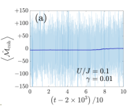
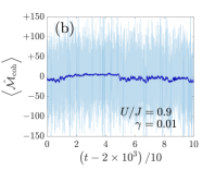
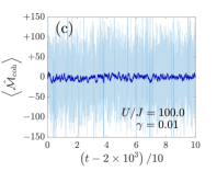
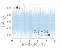
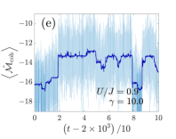
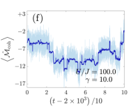
Figure 4: We plot the time dependent expectation value (68) of the measurement operator $\hat{\mathcal{M}}_{\mathrm{coh}}$ vs time in dark blue. We also plot $I(t)/(2\gamma)$ in faded blue to show the effect of the Wiener noise in the homodyne measurement signal. We see the signature of the superfluid to Mott-insulator phase transition in the time dependent dynamics of $\left\langle\hat{\mathcal{M}}_{\mathrm{coh}}\right\rangle$ in panels (a), (b) and (c). Considering $10^{3}$ times larger measurement strength in panels (d), (e) and (f), we show examples of quantum trajectories in the quantum Zeno regime. Deep in the Mott-insulating phase, we observe frequent quantum jumps in this regime.

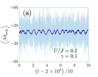
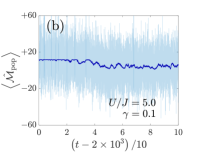
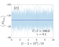
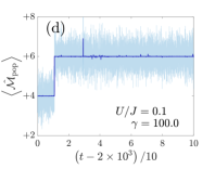
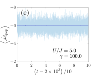
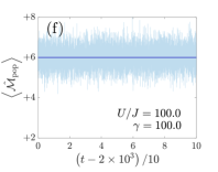
Figure 5: We show the plots for the time dependent expectation value (68) of the measurement operator $\hat{\mathcal{M}}_{\mathrm{pop}}$ vs time and $I(t)/(2\gamma)$ vs time in dark and faded blue, respectively. As expected, the superfluid dynamics here in (a) is similar to the Mott-insulator dynamics of Fig. 4(c) and vice versa. For the trajectories in the quantum Zeno regime (d)-(f), we observe fewer quantum jumps here than in Figs. 4(d)-(f).

4 An Example: The Bose-Hubbard Model

To numerically demonstrate the stochastic Schrödinger dynamics of Eq. (63), we start with the optical lattice potential

$$V_{l}(x)=V_{0}\sin^{2}(kx),$$ (65)

where the wave vector $k$ is related to the wavelength of the laser light by the relation $k=2\pi/\lambda$. Expanding the atomic field operators in terms of the Wannier functions for the optical lattice potential (65), one can show that $\hat{\mathcal{H}}_{\text{atm}}$ becomes the following Bose-Hubbard Hamiltonian [15]

$$\hat{\mathcal{H}}_{\text{BH}}=-J\sum_{\left\langle i,j\right\rangle}\hat{b}^{\dagger}_{i}\hat{b}_{j}+\sum_{i}\epsilon_{i}\hat{n}_{i}+\frac{U}{2}\sum_{i}\hat{n}_{i}(\hat{n}_{i}-1),$$ (66)

where $\hat{n}_{i}=\hat{b}^{\dagger}_{i}\hat{b}_{i}$ and the parameters of $\hat{\mathcal{H}}_{\text{BH}}$ are given by

$$J= \int w_{j}(x)^{*}\left(-\frac{\hat{p}^{2}}{2m}+V_{l}(x)\right)w_{j+1}(x)\mathrm{d}x$$ (67a)

$$U= \;\;g_{s}\int|w_{j}(x)|^{4}\mathrm{d}x,$$ (67b)

$$\epsilon_{i}\approx \;\;V_{T}(x_{i}),$$ (67c)

with $V_{l}$ the lattice potential, $V_{T}$ a slowly varying external trapping potential, and $g_{s}$ the s-wave scattering length in one-dimension.

Considering two different choices of the spatial mode function $f_{a}(x,\omega_{\text{L}})$, we obtain the two Hermitian observables $\hat{\mathcal{M}}_{0}:\hat{\mathcal{M}}_{\mathrm{coh}}=m_{\mathrm{coh}}\sum_{j}\hat{b}_{j}^{\dagger}\hat{b}_{j+1}+h.c.$ and $\hat{\mathcal{M}}_{0}:\hat{\mathcal{M}}_{\mathrm{pop}}=m_{\mathrm{pop}}\sum_{j}\hat{b}_{2j}^{\dagger}\hat{b}_{2j}$, whose weak and continuous measurements was studied in Ref. [12]. Here $m_{\mathrm{coh}}$ and $m_{\mathrm{pop}}$ are two constants calculated from the Wannier functions. The Bose-Hubbard Hamiltonian (66) has a superfluid to Mott-insulator transition at $U/J\approx 4.65$ in the thermodynamic limit [18]. The plot depicting the ground state expectation value of $\hat{\mathcal{M}}_{\mathrm{coh}}$ in Fig. 3 is consistent with this critical value.

In this section, we numerically study the stochastic Schrödinger dynamics of Eq. (63). We show the examples of individual quantum trajectories due to the coherence measurement $\hat{\mathcal{M}}_{\mathrm{coh}}$ in Fig. 4 and due to the population measurement $\hat{\mathcal{M}}_{\mathrm{pop}}$ in Fig. 5. In each of the panels of Figs. 4 and 5, we plot the time dependent expectation value of the measurement operators

$$\left\langle\hat{\mathcal{M}}_{0}\right\rangle=\left\langle\Psi(t)\right|\hat{\mathcal{M}}_{0}\left|\Psi(t)\right\rangle$$ (68)

vs time for different values of the parameter $U/J$ and different measurement strength $\gamma$, where $\left|\Psi(t)\right\rangle$ is obtained numerically from the SSE (63). Since we are not interested in the transient effects, we have not shown the trajectory upto $t=2\times 10^{3}$.

From the plots shown in Figs. 4(a)-(c) and 5(a)-(c), we conclude that signatures of the superfluid to Mott-insulator transition can even be detected in the measurement signals (without the Wiener noise) for individual quantum trajectories. The phase transition is in agreement with the one detected in Ref. [12] with the help of power spectral densities.

In Fig. 4(a), we see that the coherence measurement signal remains almost constant in the superfluid phase with $U/J=0.1$. On the other hand, in Fig. 4(c), we observe chaotic oscillations in the Mott-insulating phase with $U/J=100.0$. Interestingly, the coherence measurement appears to be able to distinguish the phases even in the strong measurement (quantum Zeno) regime at $\gamma=10.0$. This is in stark contrast to the coherence measurement PSDs obtained for the quantum Zeno regime in Ref. [12]. However, one must point out that the nature of the stochastic jumps in Figs. 4(e) and (f) are quite different from the chaotic fluctuations observed in Figs. 4(b) and (c).

In the weak measurement regime, one observes chaotic fluctuations in the population measurement signal in the superfluid phase in Fig. 5(a) and almost constant signal in the Mott-insulator phase Fig. 5(c). It is hard to distinguish the phases using the population signals in the quantum Zeno regime that are shown in 5(d)-(f). Our study shows that typical quantum trajectories from different measurement signals contain a lot of information even in the quantum Zeno regime.

5 Conclusion

Starting from a full atom-light Hamiltonian, we derive an SSE solely in terms of the atomic degrees of freedom. The SSE is conditioned upon a homodyne measurement record. We explain how the approaches of Refs. [7], [8], [9] and the one adopted in Ref. [14] could be reconciled. This then demonstrates that, in general, a homodyne measurement setup with a linear coupling between a Hermitian atomic measurement operator and the coherent probe laser leads to a Gaussian quantum continuous measurement.

Appendix A Evaluation of Important Gaussian Integrals

We show the details of how to compute the Gaussian integrals appearing in Eqs. (46) and (56) in this appendix. In both examples, we replace the summation over photon number $p$ by an integral with lower and upper limit of $0$ and $\infty$, respectively.

A.1 Gaussian Integral Needed to Simplify the Probability $P_{k}$

Here we consider the summation that appears on the last line of Eq. (46). We replace the summation over $p$ by an integration and obtain

$$\begin{aligned} &\sum_{p=0}^{\infty}\frac{1}{2\pi\left|\alpha_{m}^{\prime}\right|\left|\beta_{m}^{\prime}\right|}\exp{\left(-\frac{(p+k-\left|\alpha_{m}^{\prime}\right|^{2})^{2}}{2\left|\alpha_{m}^{\prime}\right|^{2}}-\frac{(p-\left|\beta_{m}^{\prime}\right|^{2})^{2}}{2\left|\beta_{m}^{\prime}\right|^{2}}\right)}\\ &\approx\int_{0}^{\infty}\mathrm{d}p\frac{1}{2\pi\left|\alpha_{m}^{\prime}\right|\left|\beta_{m}^{\prime}\right|}\exp{\left(-\frac{(p+k-\left|\alpha_{m}^{\prime}\right|^{2})^{2}}{2\left|\alpha_{m}^{\prime}\right|^{2}}-\frac{(p-\left|\beta_{m}^{\prime}\right|^{2})^{2}}{2\left|\beta_{m}^{\prime}\right|^{2}}\right)}\\ &=\exp{\left[-\frac{\left(k+\left|\beta_{m}^{\prime}\right|^{2}-\left|\alpha_{m}^{\prime}\right|^{2}\right)^{2}}{2\left(\left|\beta_{m}^{\prime}\right|^{2}+\left|\alpha_{m}^{\prime}\right|^{2}\right)}\right]}\times\int_{\frac{\left|\beta_{m}^{\prime}\right|^{2}\left(k-2\left|\alpha_{m}^{\prime}\right|^{2}\right)}{\left|\beta_{m}^{\prime}\right|^{2}+\left|\alpha_{m}^{\prime}\right|^{2}}}^{\infty}\mathrm{d}\widetilde{p}\frac{1}{2\pi\left|\alpha_{m}^{\prime}\right|\left|\beta_{m}^{\prime}\right|}\exp{\left[-\left(\frac{\left|\beta_{m}^{\prime}\right|^{2}+\left|\alpha_{m}^{\prime}\right|^{2}}{2\left|\beta_{m}^{\prime}\right|^{2}\left|\alpha_{m}^{\prime}\right|^{2}}\right)\widetilde{p}^{2}\right]},\end{aligned}$$ (69)

where we have introduced a new shifted variable

$$\widetilde{p}=p+\frac{\left|\beta_{m}^{\prime}\right|^{2}\left(k-2\left|\alpha_{m}^{\prime}\right|^{2}\right)}{\left|\beta_{m}^{\prime}\right|^{2}+\left|\alpha_{m}^{\prime}\right|^{2}}.$$ (70)

Since $\left|\alpha_{m}^{\prime}\right|^{2},\left|\beta_{m}^{\prime}\right|^{2}\gg 1$, we have

$$\frac{\left|\beta_{m}^{\prime}\right|^{2}\left(k-2\left|\alpha_{m}^{\prime}\right|^{2}\right)}{\left|\beta_{m}^{\prime}\right|^{2}+\left|\alpha_{m}^{\prime}\right|^{2}}\approx-\frac{2\left|\alpha_{m}^{\prime}\right|^{2}\left|\beta_{m}^{\prime}\right|^{2}}{\left|\beta_{m}^{\prime}\right|^{2}+\left|\alpha_{m}^{\prime}\right|^{2}}\rightarrow-\infty.$$ (71)

Using the above, we extend the lower limit of the integration to $-\infty$ in Eq. (69) and finally obtain

$$\begin{aligned} &\sum_{p=0}^{\infty}\frac{1}{2\pi\left|\alpha_{m}^{\prime}\right|\left|\beta_{m}^{\prime}\right|}\exp{\left(-\frac{(p+k-\left|\alpha_{m}^{\prime}\right|^{2})^{2}}{2\left|\alpha_{m}^{\prime}\right|^{2}}-\frac{(p-\left|\beta_{m}^{\prime}\right|^{2})^{2}}{2\left|\beta_{m}^{\prime}\right|^{2}}\right)}\\ &\approx\frac{1}{2\pi\left|\alpha_{m}^{\prime}\right|\left|\beta_{m}^{\prime}\right|}\exp{\left[-\frac{\left(k+\left|\beta_{m}^{\prime}\right|^{2}-\left|\alpha_{m}^{\prime}\right|^{2}\right)^{2}}{2\left(\left|\beta_{m}^{\prime}\right|^{2}+\left|\alpha_{m}^{\prime}\right|^{2}\right)}\right]}\int_{-\infty}^{+\infty}\mathrm{d}\widetilde{p}\exp{\left[-\left(\frac{\left|\beta_{m}^{\prime}\right|^{2}+\left|\alpha_{m}^{\prime}\right|^{2}}{2\left|\beta_{m}^{\prime}\right|^{2}\left|\alpha_{m}^{\prime}\right|^{2}}\right)\widetilde{p}^{2}\right]}\\ &=\frac{1}{\sqrt{2\pi\left(\left|\beta_{m}^{\prime}\right|^{2}+\left|\alpha_{m}^{\prime}\right|^{2}\right)}}\exp{\left[-\frac{\left(k+\left|\beta_{m}^{\prime}\right|^{2}-\left|\alpha_{m}^{\prime}\right|^{2}\right)^{2}}{2\left(\left|\beta_{m}^{\prime}\right|^{2}+\left|\alpha_{m}^{\prime}\right|^{2}\right)}\right]}.\end{aligned}$$ (72)

A.2 Gaussian Integral Needed to Simplify the Density Matrix $\rho(t+\mathrm{d}t)$

We consider the summation that appears on the last line of Eq. (56). Replacing the summation over $p$ by an integration, we obtain

$$\begin{aligned} &\sum_{p}\exp\left[-\frac{(p-\left|\beta_{m}^{\prime}\right|^{2})^{2}}{4\left|\beta_{m}^{\prime}\right|^{2}}-\frac{(p-\left|\beta_{n}^{\prime}\right|^{2})^{2}}{4\left|\beta_{n}^{\prime}\right|^{2}}-\frac{(p+k-\left|\alpha_{m}^{\prime}\right|^{2})^{2}}{4\left|\alpha_{m}^{\prime}\right|^{2}}-\frac{(p+k-\left|\alpha_{n}^{\prime}\right|^{2})^{2}}{4\left|\alpha_{n}^{\prime}\right|^{2}}-p\theta\right]\\ &\approx\int_{0}^{\infty}\mathrm{d}p\;\;\exp\left[-\frac{(p-\left|\beta_{m}^{\prime}\right|^{2})^{2}}{4\left|\beta_{m}^{\prime}\right|^{2}}-\frac{(p-\left|\beta_{n}^{\prime}\right|^{2})^{2}}{4\left|\beta_{n}^{\prime}\right|^{2}}-\frac{(p+k-\left|\alpha_{m}^{\prime}\right|^{2})^{2}}{4\left|\alpha_{m}^{\prime}\right|^{2}}-\frac{(p+k-\left|\alpha_{n}^{\prime}\right|^{2})^{2}}{4\left|\alpha_{n}^{\prime}\right|^{2}}-p\theta\right],\end{aligned}$$ (73)

where $\theta$ will be computed in B. After completing the square in the argument of the exponential in Eq. (73), we note that

$$\begin{aligned} &\frac{(p-\left|\beta_{m}^{\prime}\right|^{2})^{2}}{4\left|\beta_{m}^{\prime}\right|^{2}}+\frac{(p-\left|\beta_{n}^{\prime}\right|^{2})^{2}}{4\left|\beta_{n}^{\prime}\right|^{2}}+\frac{(p+k-\left|\alpha_{m}^{\prime}\right|^{2})^{2}}{4\left|\alpha_{m}^{\prime}\right|^{2}}+\frac{(p+k-\left|\alpha_{n}^{\prime}\right|^{2})^{2}}{4\left|\alpha_{n}^{\prime}\right|^{2}}+p\theta\\ &=\frac{1}{4}\left[\left(\left|\beta_{m}^{\prime}\right|^{2}+\left|\beta_{n}^{\prime}\right|^{2}+\left|\alpha_{m}^{\prime}\right|^{2}+\left|\alpha_{n}^{\prime}\right|^{2}\right)-4k+\frac{k^{2}}{\left|\alpha_{m}^{\prime}\right|^{2}}+\frac{k^{2}}{\left|\alpha_{n}^{\prime}\right|^{2}}\right.\\ &\left.-\frac{\left|\beta_{m}^{\prime}\right|^{2}\left|\beta_{n}^{\prime}\right|^{2}\left[2\left|\alpha_{m}^{\prime}\right|^{2}\left|\alpha_{n}^{\prime}\right|^{2}\left(\theta-2\right)+\left(\left|\alpha_{m}^{\prime}\right|^{2}+\left|\alpha_{n}^{\prime}\right|^{2}\right)k\right]^{2}}{\left|\alpha_{m}^{\prime}\right|^{2}\left|\alpha_{n}^{\prime}\right|^{2}\left[\left|\alpha_{m}^{\prime}\right|^{2}\left|\alpha_{n}^{\prime}\right|^{2}\left(\left|\beta_{m}^{\prime}\right|^{2}+\left|\beta_{n}^{\prime}\right|^{2}\right)+\left|\beta_{m}^{\prime}\right|^{2}\left|\beta_{n}^{\prime}\right|^{2}\left(\left|\alpha_{m}^{\prime}\right|^{2}+\left|\alpha_{n}^{\prime}\right|^{2}\right)\right]}\right]\\ &+\frac{1}{4}\left(\frac{1}{\left|\beta_{m}^{\prime}\right|^{2}}+\frac{1}{\left|\beta_{n}^{\prime}\right|^{2}}+\frac{1}{\left|\alpha_{m}^{\prime}\right|^{2}}+\frac{1}{\left|\alpha_{n}^{\prime}\right|^{2}}\right)\left(\frac{\left|\beta_{m}^{\prime}\right|^{2}\left|\beta_{n}^{\prime}\right|^{2}\left[2\left|\alpha_{m}^{\prime}\right|^{2}\left|\alpha_{n}^{\prime}\right|^{2}\left(\theta-2\right)+\left(\left|\alpha_{m}^{\prime}\right|^{2}+\left|\alpha_{n}^{\prime}\right|^{2}\right)k\right]}{\left|\alpha_{m}^{\prime}\right|^{2}\left|\alpha_{n}^{\prime}\right|^{2}\left(\left|\beta_{m}^{\prime}\right|^{2}+\left|\beta_{n}^{\prime}\right|^{2}\right)+\left|\beta_{m}^{\prime}\right|^{2}\left|\beta_{n}^{\prime}\right|^{2}\left(\left|\alpha_{m}^{\prime}\right|^{2}+\left|\alpha_{n}^{\prime}\right|^{2}\right)}+p\right)^{2}\\ &\equiv Q_{1}(k)+Q_{20}\left(Q_{21}+p\right)^{2},\end{aligned}$$ (74)

where in the last line we have defined new variables $Q_{1},Q_{20},$ and $Q_{21}$. In particular, we define

$$Q_{1}(k)=\frac{1}{4}\left[\left(\left|\beta_{m}^{\prime}\right|^{2}+\left|\beta_{n}^{\prime}\right|^{2}+\left|\alpha_{m}^{\prime}\right|^{2}+\left|\alpha_{n}^{\prime}\right|^{2}\right)-4k+\frac{k^{2}}{\left|\alpha_{m}^{\prime}\right|^{2}}+\frac{k^{2}}{\left|\alpha_{n}^{\prime}\right|^{2}}\right.\\ \left.-\frac{\left|\beta_{m}^{\prime}\right|^{2}\left|\beta_{n}^{\prime}\right|^{2}\left[2\left|\alpha_{m}^{\prime}\right|^{2}\left|\alpha_{n}^{\prime}\right|^{2}\left(\theta-2\right)+\left(\left|\alpha_{m}^{\prime}\right|^{2}+\left|\alpha_{n}^{\prime}\right|^{2}\right)k\right]^{2}}{\left|\alpha_{m}^{\prime}\right|^{2}\left|\alpha_{n}^{\prime}\right|^{2}\left[\left|\alpha_{m}^{\prime}\right|^{2}\left|\alpha_{n}^{\prime}\right|^{2}\left(\left|\beta_{m}^{\prime}\right|^{2}+\left|\beta_{n}^{\prime}\right|^{2}\right)+\left|\beta_{m}^{\prime}\right|^{2}\left|\beta_{n}^{\prime}\right|^{2}\left(\left|\alpha_{m}^{\prime}\right|^{2}+\left|\alpha_{n}^{\prime}\right|^{2}\right)\right]}\right]$$ (75)

to be a quadratic polynomial in $k$ that does not depend on $p$. As a result, one can pull the factor $\exp\left[-Q_{1}(k)\right]$ out of the summation in Eq. (73).

Using the variables introduced in Eq. (74), we obtain from Eq. (73)

$$\begin{aligned} &\exp\left[Q_{1}(k)\right]\times\sum_{p}\exp\left[-\frac{(p-\left|\beta_{m}^{\prime}\right|^{2})^{2}}{4\left|\beta_{m}^{\prime}\right|^{2}}-\frac{(p-\left|\beta_{n}^{\prime}\right|^{2})^{2}}{4\left|\beta_{n}^{\prime}\right|^{2}}-\frac{(p+k-\left|\alpha_{m}^{\prime}\right|^{2})^{2}}{4\left|\alpha_{m}^{\prime}\right|^{2}}-\frac{(p+k-\left|\alpha_{n}^{\prime}\right|^{2})^{2}}{4\left|\alpha_{n}^{\prime}\right|^{2}}-p\theta\right]\\ &=\int_{0}^{\infty}\mathrm{d}p\;\exp{\left[-Q_{20}\left(Q_{21}+p\right)^{2}\right]}\\ &=\int_{Q_{21}^{\textrm{Re}}(k)}^{\infty}\mathrm{d}\widetilde{p}_{1}\;\exp{\left[-Q_{20}\left(Q_{21}^{\theta}(k)+\widetilde{p}_{1}\right)^{2}\right]},\end{aligned}$$ (76)

where we have introduced the variable change

$$\widetilde{p}_{1}\equiv p+Q_{21}^{\textrm{Re}}(k)=p+\frac{\left|\beta_{m}^{\prime}\right|^{2}\left|\beta_{n}^{\prime}\right|^{2}\left[k\left(\left|\alpha_{m}^{\prime}\right|^{2}+\left|\alpha_{n}^{\prime}\right|^{2}\right)-4\left|\alpha_{m}^{\prime}\right|^{2}\left|\alpha_{n}^{\prime}\right|^{2}\right]}{\left|\alpha_{m}^{\prime}\right|^{2}\left|\alpha_{n}^{\prime}\right|^{2}\left(\left|\beta_{m}^{\prime}\right|^{2}+\left|\beta_{n}^{\prime}\right|^{2}\right)+\left|\beta_{m}^{\prime}\right|^{2}\left|\beta_{n}^{\prime}\right|^{2}\left(\left|\alpha_{m}^{\prime}\right|^{2}+\left|\alpha_{n}^{\prime}\right|^{2}\right)}.$$ (77)

The shift $Q_{21}^{\textrm{Re}}(k)$ becomes the new lower limit of the integral. Inside the integrand, we have introduced the new variable

$$Q_{21}^{\theta}(k)\equiv Q_{21}(k)-Q_{21}^{\textrm{Re}}(k)=\frac{2\theta\left|\alpha_{m}^{\prime}\right|^{2}\left|\alpha_{n}^{\prime}\right|^{2}\left|\beta_{m}^{\prime}\right|^{2}\left|\beta_{n}^{\prime}\right|^{2}}{\left|\alpha_{m}^{\prime}\right|^{2}\left|\alpha_{n}^{\prime}\right|^{2}\left(\left|\beta_{m}^{\prime}\right|^{2}+\left|\beta_{n}^{\prime}\right|^{2}\right)+\left|\beta_{m}^{\prime}\right|^{2}\left|\beta_{n}^{\prime}\right|^{2}\left(\left|\alpha_{m}^{\prime}\right|^{2}+\left|\alpha_{n}^{\prime}\right|^{2}\right)}$$ (78)

for convenience. Since $\theta$ is complex, $Q_{21}^{\theta}(k)$ is also a complex number.

Similar to (71), we can replace the lower limit of the integral $Q_{21}^{\textrm{Re}}(k)$ by $-\infty$ using the fact $\left|\alpha_{m}^{\prime}\right|^{2},\left|\alpha_{n}^{\prime}\right|^{2},\left|\beta_{m}^{\prime}\right|^{2},\left|\beta_{n}^{\prime}\right|^{2}\gg 1$. This then obtains from Eq. (76) the following Gaussian integral offset by a $Q_{21}^{\theta}(k)$:

$$\int_{Q_{21}^{\textrm{Re}}(k)}^{\infty}\mathrm{d}\widetilde{p}_{1}\;\exp{\left[-Q_{20}\left(Q_{21}^{\theta}(k)+\widetilde{p}_{1}\right)^{2}\right]}\approx\int_{-\infty}^{\infty}\mathrm{d}\widetilde{p}_{1}\;\exp{\left[-Q_{20}\left(Q_{21}^{\theta}(k)+\widetilde{p}_{1}\right)^{2}\right]}\\ =\sqrt{\frac{\pi}{Q_{20}}}=\frac{\sqrt{4\pi}}{\left(\frac{1}{\left|\beta_{m}^{\prime}\right|^{2}}+\frac{1}{\left|\beta_{n}^{\prime}\right|^{2}}+\frac{1}{\left|\alpha_{m}^{\prime}\right|^{2}}+\frac{1}{\left|\alpha_{n}^{\prime}\right|^{2}}\right)^{\frac{1}{2}}},$$ (79)

which produces the same result as a usual Gaussian integral. As a result, we finally have

$$\sum_{p}\exp\left[-\frac{(p-\left|\beta_{m}^{\prime}\right|^{2})^{2}}{4\left|\beta_{m}^{\prime}\right|^{2}}-\frac{(p-\left|\beta_{n}^{\prime}\right|^{2})^{2}}{4\left|\beta_{n}^{\prime}\right|^{2}}-\frac{(p+k-\left|\alpha_{m}^{\prime}\right|^{2})^{2}}{4\left|\alpha_{m}^{\prime}\right|^{2}}-\frac{(p+k-\left|\alpha_{n}^{\prime}\right|^{2})^{2}}{4\left|\alpha_{n}^{\prime}\right|^{2}}-p\theta\right]\\ \approx\frac{\sqrt{4\pi}}{\left(\frac{1}{\left|\beta_{m}^{\prime}\right|^{2}}+\frac{1}{\left|\beta_{n}^{\prime}\right|^{2}}+\frac{1}{\left|\alpha_{m}^{\prime}\right|^{2}}+\frac{1}{\left|\alpha_{n}^{\prime}\right|^{2}}\right)^{\frac{1}{2}}}\exp\left[-Q_{1}(k)\right],$$ (80)

where $Q_{1}(k)$ is defined in Eq. (75).

Appendix B Approximate Value of $\theta$ Introduced in Eq. (57)

In this section, we compute the value of $\theta$ introduced in Eq. (57) while keeping terms upto $\mathcal{O}(\mathrm{d}t)$ and $\mathcal{O}\left(\alpha_{0}\beta/\left(\alpha^{2}+\beta^{2}\right)\right)$. Recall the definition

$$\begin{split}i\theta&=\mathrm{Arg}(\beta_{m}^{\prime})+\mathrm{Arg}(\beta_{n}^{\prime*})+\mathrm{Arg}(\alpha_{m}^{\prime})+\mathrm{Arg}(\alpha_{n}^{\prime*})\\ &=-\tan^{-1}\left(\frac{\beta+\alpha_{0}m\mathrm{d}t}{\alpha}\right)+\tan^{-1}\left(\frac{\beta+\alpha_{0}n\mathrm{d}t}{\alpha}\right)+\tan^{-1}\left(\frac{\beta-\alpha_{0}m\mathrm{d}t}{\alpha}\right)-\tan^{-1}\left(\frac{\beta-\alpha_{0}n\mathrm{d}t}{\alpha}\right),\end{split}$$ (81)

where $-\pi/2\leqslant\mathrm{Arg}(\beta_{m}^{\prime}),\mathrm{Arg}(\beta_{n}^{\prime*}),\mathrm{Arg}(\alpha_{m}^{\prime}),\mathrm{Arg}(\alpha_{n}^{\prime*})<+\pi/2$. Using the formula

$$\tan^{-1}(x)-\tan^{-1}(y)=\tan^{-1}\left(\frac{x-y}{1+xy}\right)$$ (82)

and neglecting terms $\mathcal{O}(\mathrm{d}t^{2})$ in the denominator, we obtain

$$-\tan^{-1}\left(\frac{\beta+\alpha_{0}m\mathrm{d}t}{\alpha}\right)+\tan^{-1}\left(\frac{\beta+\alpha_{0}n\mathrm{d}t}{\alpha}\right)=\tan^{-1}\left(\frac{\alpha\alpha_{0}(n-m)\mathrm{d}t}{\alpha^{2}+\beta^{2}+\alpha_{0}\beta(m+n)\mathrm{d}t}\right).$$ (83)

Simplifying the other two terms in Eq. (81) similarly, we write

$$\begin{split}i\theta&=\tan^{-1}\left(\frac{\alpha\alpha_{0}(n-m)\mathrm{d}t}{\alpha^{2}+\beta^{2}+\alpha_{0}\beta(m+n)\mathrm{d}t}\right)+\tan^{-1}\left(\frac{\alpha\alpha_{0}(n-m)\mathrm{d}t}{\alpha^{2}+\beta^{2}-\alpha_{0}\beta(m+n)\mathrm{d}t}\right)\\ &\approx\tan^{-1}\left[\frac{\alpha\alpha_{0}(n-m)\mathrm{d}t}{\alpha^{2}+\beta^{2}}\left(1-\frac{\alpha_{0}\beta(m+n)\mathrm{d}t}{\alpha^{2}+\beta^{2}}\right)\right]+\tan^{-1}\left[\frac{\alpha\alpha_{0}(n-m)\mathrm{d}t}{\alpha^{2}+\beta^{2}}\left(1+\frac{\alpha_{0}\beta(m+n)\mathrm{d}t}{\alpha^{2}+\beta^{2}}\right)\right]\\ &\approx 2\tan^{-1}\left(\frac{\alpha\alpha_{0}(n-m)\mathrm{d}t}{\alpha^{2}+\beta^{2}}\right)\\ &\approx 2\left(\frac{\alpha\alpha_{0}(n-m)\mathrm{d}t}{\alpha^{2}+\beta^{2}}\right).\end{split}$$ (84)

In Eq. (84) we have used the following Taylor series expansions for $-1\leqslant x\leqslant+1$:

$$\tan^{-1}(x)=\sum_{n=0}^{\infty}(-1)^{n}\frac{x^{2n+1}}{2n+1},\qquad\frac{1}{1-x}=\sum_{n=0}^{\infty}x^{n},$$ (85)

and kept terms upto $\mathcal{O}(\mathrm{d}t)$.

Appendix C Simplification of the Density Matrix $\rho(t+\mathrm{d}t)$

In this section, we simplify $\rho(t+\mathrm{d}t)$ and finally write it as a rank-1 projector. Using Eq. (80) in Eq. (56), we derive

$$\begin{aligned} \rho(t+\mathrm{d}t)&=\left|\Psi(t+\mathrm{d}t)\right\rangle\left\langle\Psi(t+\mathrm{d}t)\right|\\ &\approx\sum_{m,n}\frac{\sqrt{4\pi}C_{m}C_{n}^{*}e^{-i\alpha_{0}\alpha(m-n)\mathrm{d}t}\left[e^{-i\hat{\widetilde{\mathcal{H}}}_{\text{atm}}\mathrm{d}t}\left|\psi_{m}\right\rangle\left\langle\psi_{n}\right|e^{+i\hat{\widetilde{\mathcal{H}}}_{\text{atm}}\mathrm{d}t}\right]}{2\pi P_{k}\left[\left|\beta_{m}^{\prime}\right|^{2}\left|\beta_{n}^{\prime}\right|^{2}\left|\alpha_{m}^{\prime}\right|^{2}\left|\alpha_{n}^{\prime}\right|^{2}\right]^{\frac{1}{4}}\left(\frac{1}{\left|\beta_{m}^{\prime}\right|^{2}}+\frac{1}{\left|\beta_{n}^{\prime}\right|^{2}}+\frac{1}{\left|\alpha_{m}^{\prime}\right|^{2}}+\frac{1}{\left|\alpha_{n}^{\prime}\right|^{2}}\right)^{\frac{1}{2}}}\exp\left[-Q_{1}(k)\right]\\ &\approx\sum_{m,n}\frac{C_{m}C_{n}^{*}e^{-i\alpha_{0}\alpha(m-n)\mathrm{d}t}\left[e^{-i\hat{\widetilde{\mathcal{H}}}_{\text{atm}}\mathrm{d}t}\left|\psi_{m}\right\rangle\left\langle\psi_{n}\right|e^{+i\hat{\widetilde{\mathcal{H}}}_{\text{atm}}\mathrm{d}t}\right]}{P_{k}\left[2\pi\left(\alpha^{2}+\beta^{2}\right)\right]^{\frac{1}{2}}}\exp\left[-Q_{1}(k)\right],\end{aligned}$$ (86)

where we have used

$$\left|\beta_{m}^{\prime}\right|^{2}\left|\beta_{n}^{\prime}\right|^{2}\left|\alpha_{m}^{\prime}\right|^{2}\left|\alpha_{n}^{\prime}\right|^{2}\approx\frac{1}{16}\left(\alpha^{2}+\beta^{2}\right)^{4},\qquad\left(\frac{1}{\left|\beta_{m}^{\prime}\right|^{2}}+\frac{1}{\left|\beta_{n}^{\prime}\right|^{2}}+\frac{1}{\left|\alpha_{m}^{\prime}\right|^{2}}+\frac{1}{\left|\alpha_{n}^{\prime}\right|^{2}}\right)\approx\frac{8}{\alpha^{2}+\beta^{2}},$$ (87)

after neglecting $\mathcal{O}(\mathrm{d}t^{2})$ terms.

We now simplify $Q_{1}(k)$ from Eq. (75) by neglecting $\mathcal{O}(\mathrm{d}t^{2})$ terms as

$$\begin{aligned} Q_{1}(k)&\approx\frac{k^{2}}{\alpha^{2}+\beta^{2}}\left(\frac{1}{2}-\frac{4\alpha_{0}\beta(m+n)\mathrm{d}t}{\alpha^{2}+\beta^{2}}\right)+k\frac{\left\{i\alpha_{0}\alpha(n-m)\mathrm{d}t+\alpha_{0}\beta(m+n)\mathrm{d}t\right\}}{\left(\alpha^{2}+\beta^{2}\right)}-i\alpha_{0}\alpha(n-m)\mathrm{d}t\\ &\overset{*1}{\approx}\frac{k^{2}+2k\left\{i\alpha_{0}\alpha(n-m)\mathrm{d}t+\alpha_{0}\beta(m+n)\mathrm{d}t\right\}}{2\left(\alpha^{2}+\beta^{2}\right)}-i\alpha_{0}\alpha(n-m)\mathrm{d}t\\ &\overset{*2}{\approx}\frac{k^{2}+2k\alpha_{0}\beta(m+n)\mathrm{d}t}{2\left(\alpha^{2}+\beta^{2}\right)}-i\alpha_{0}\alpha(n-m)\mathrm{d}t.\end{aligned}$$ (88)

Since $\beta^{2}=\mathcal{O}(1/\mathrm{d}t)\gg 1$, in the second line ($*1$) of Eq. (88) we have neglected the term that is proportional to $\alpha_{0}\beta/\left(\alpha^{2}+\beta^{2}\right)^{2}$ in the coefficient of $k^{2}$. Moreover, since the probe light is quite weak compared to the local oscillator, we also neglect $\alpha_{0}\alpha/\left(\alpha^{2}+\beta^{2}\right)$ compared to $\alpha_{0}\beta/\left(\alpha^{2}+\beta^{2}\right)$ in the final line ($*2$).

First neglecting the constant factor $P_{k}\sqrt{\left[2\pi\left(\alpha^{2}+\beta^{2}\right)\right]}$ and then using Eq. (88) into (86), we obtain

$$\begin{aligned} \rho(t+\mathrm{d}t)&=\left|\Psi(t+\mathrm{d}t)\right\rangle\left\langle\Psi(t+\mathrm{d}t)\right|\\ &\propto\sum_{m,n}C_{m}C_{n}^{*}e^{-i\alpha_{0}\alpha(m-n)\mathrm{d}t}\left[e^{-i\hat{\widetilde{\mathcal{H}}}_{\text{atm}}\mathrm{d}t}\left|\psi_{m}\right\rangle\left\langle\psi_{n}\right|e^{+i\hat{\widetilde{\mathcal{H}}}_{\text{atm}}\mathrm{d}t}\right]\exp\left[-Q_{1}(k)\right]\\ &\approx\sum_{m,n}C_{m}C_{n}^{*}e^{-i\alpha_{0}\alpha(m-n)\mathrm{d}t}e^{\left[-\frac{k^{2}+2k\alpha_{0}\beta(m+n)\mathrm{d}t}{2\left(\alpha^{2}+\beta^{2}\right)}+i\alpha_{0}\alpha(n-m)\mathrm{d}t\right]}\left[e^{-i\hat{\widetilde{\mathcal{H}}}_{\text{atm}}\mathrm{d}t}\left|\psi_{m}\right\rangle\left\langle\psi_{n}\right|e^{+i\hat{\widetilde{\mathcal{H}}}_{\text{atm}}\mathrm{d}t}\right]\\ &\approx\sum_{m,n}\left[C_{m}C_{n}^{*}e^{-i\hat{\mathcal{H}}^{\text{eff}}_{\text{atm}}\mathrm{d}t}\left|\psi_{m}\right\rangle\left\langle\psi_{n}\right|e^{+i\hat{\mathcal{H}}^{\text{eff}}_{\text{atm}}\mathrm{d}t}\right]\exp\left[-\frac{\left\{2k^{2}+4k\alpha_{0}\beta(m+n)\mathrm{d}t\right\}}{4(\alpha^{2}+\beta^{2})}\right]\\ &\approx\sum_{m,n}C_{m}C_{n}^{*}e^{-i\hat{\mathcal{H}}^{\text{eff}}_{\text{atm}}\mathrm{d}t}e^{-\frac{\left[k+2\alpha_{0}\beta m\mathrm{d}t\right]^{2}}{4\left[\alpha^{2}+\beta^{2}\right]}}\left|\psi_{m}\right\rangle\left\langle\psi_{n}\right|e^{-\frac{\left[k+2\alpha_{0}\beta n\mathrm{d}t\right]^{2}}{4\left[\alpha^{2}+\beta^{2}\right]}}e^{+i\hat{\mathcal{H}}^{\text{eff}}_{\text{atm}}\mathrm{d}t}\\ &=e^{-i\hat{\mathcal{H}}^{\text{eff}}_{\text{atm}}\mathrm{d}t}e^{-\frac{\left[\hat{k}+2\alpha_{0}\beta\hat{\mathcal{M}}\mathrm{d}t\right]^{2}}{4\left[\alpha^{2}+\beta^{2}\right]}}\left[\sum_{m,n}C_{m}C_{n}^{*}\left|\psi_{m}\right\rangle\left\langle\psi_{n}\right|\right]e^{-\frac{\left[\hat{k}+2\alpha_{0}\beta\hat{\mathcal{M}}\mathrm{d}t\right]^{2}}{4\left[\alpha^{2}+\beta^{2}\right]}}e^{+i\hat{\mathcal{H}}^{\text{eff}}_{\text{atm}}\mathrm{d}t}\\ &=e^{-i\hat{\mathcal{H}}^{\text{eff}}_{\text{atm}}\mathrm{d}t}e^{-\frac{\left[\hat{k}+2\alpha_{0}\beta\hat{\mathcal{M}}\mathrm{d}t\right]^{2}}{4\left[\alpha^{2}+\beta^{2}\right]}}\left|\Psi(t)\right\rangle\left\langle\Psi(t)\right|e^{-\frac{\left[\hat{k}+2\alpha_{0}\beta\hat{\mathcal{M}}\mathrm{d}t\right]^{2}}{4\left[\alpha^{2}+\beta^{2}\right]}}e^{+i\hat{\mathcal{H}}^{\text{eff}}_{\text{atm}}\mathrm{d}t},\end{aligned}$$ (89)

where

$$\hat{\mathcal{H}}_{\text{atm}}^{\text{eff}}=\hat{\widetilde{\mathcal{H}}}_{\text{atm}}+2\alpha_{0}\alpha\hat{\mathcal{M}}.$$ (90)

References

References

• [1] I. Bloch, J. Dalibard, and W. Zwerger, Many-body physics with ultracold gases, Rev. Mod. Phys. 80, 885 (2008).
• [2] M. Greiner, O. Mandel, T. Esslinger, T. W. Hänsch, and I. Bloch, Quantum phase transition from a superfluid to a Mott insulator in a gas of ultracold atoms, Nature 415, 39 (2002).
• [3] M. R. Dennis and J. B. Götte, Observation of the Spin Hall Effect of Light via Weak Measurements, Science 319, 787 (2008).
• [4] M. R. Dennis and J. B. Götte, The analogy between optical beam shifts and quantum weak measurements, New J. Phys. 14, 073013 (2012).
• [5] S. Goswami, M. Pal, A. Nandi, P. K. Panigrahi, and N. Ghosh, Simultaneous weak value amplification of angular Goos-Hänchen and Imbert-Fedorov shifts in partial reflection, Opt. Lett. 39, 6229 (2014).
• [6] S. Goswami, M. Pal, A. Nandi, P. K. Panigrahi, and N. Ghosh, Optimized weak measurements of Goos-Hänchen and Imbert-Fedorov shifts in partial reflection, Opt. Express 24, 6041 (2016).
• [7] K. Jacobs and D. A. Steck, A Straightforward Introduction to Continuous Quantum Measurement, Contemp. Phys. 47, 279 (2006).
• [8] K. Jacobs, “Quantum measurement theory and its applications”, Cambridge University Press (2014).
• [9] H. M. Wiseman and G. J. Milburn, “Quantum measurement and control”, Cambridge University Press, New York, (2010).
• [10] K. Mølmer, Y. Castin, and J. Dalibard, Monte Carlo wave-function method in quantum optics, J. Opt. Soc. Am. B 10, 524 (1993).
• [11] K. Mølmer and Y. Castin, Monte Carlo wavefunctions in quantum optics, Quantum Semiclass. Opt. 8, 49 (1996).
• [12] A. Patra, L. F. Buchmann, F. Motzoi, K. Mølmer, J. Sherson, and A. E. B. Nielsen, Single-Shot Determination of Quantum Phases via Continuous Measurements, arXiv:1906.02518.
• [13] C. W. Gardiner and M. J. Collett, Input and output in damped quantum systems: Quantum stochastic differential equations and the master equation, Phys. Rev. A 31, 3761 (1985).
• [14] A. E. B. Nielsen and K. Mølmer, Stochastic master equation for a probed system in a cavity, Phys. Rev. A 77, 052111 (2008).
• [15] D. Jaksch, C. Bruder, J. I. Cirac, C. W. Gardiner, and P. Zoller, Cold Bosonic Atoms in Optical Lattices, Phys. Rev. Lett. 81, 3108 (1998).
• [16] M. G. A. Paris, Displacement operator by beam splitter Physics Letters A 217, 78 (1996).
• [17] C. Gerry and P. Knight, Introductory Quantum Optics, Cambridge University Press, Cambridge (2005)
• [18] J. M. Zhang and R. X. Dong, Exact diagonalization: the Bose-Hubbard model as an example, Eur. J. Phys. 31, 591 (2010).
• [19] B. Misra and E. C. G. Sudarshan, The Zeno’s paradox in quantum theory, J. Math. Phys. 18, 756 (1977).
• [20] G. A. Álvarez, E. P. Danieli, P. R. Levstein, and H. M. Pastawski, Environmentally induced quantum dynamical phase transition in the spin swapping operation, J. Chem. Phys. 124, 194507 (2006).
• [21] R. Blattmann and K. Mølmer, Conditioned quantum motion of an atom in a continuously monitored one-dimensional lattice, Phys. Rev. A 93, 052113 (2016).
• [22] D. Das, S. Dattagupta, S. Gupta, Quantum unitary evolution interspersed with repeated non-unitary interactions at random times: The method of stochastic Liouville equation, and two examples of interactions in the context of a tight-binding chain, J. Stat. Mech. 2022, 053101 (2022).