Independence Tests for Language Models

Abstract

We consider the following problem: given the weights of two models, can we test whether they were trained independently—i.e., from independent random initializations? We consider two settings: constrained and unconstrained. In the constrained setting, we make assumptions about model architecture and training and propose a family of statistical tests that yield exact p-values with respect to the null hypothesis that the models are trained from independent random initializations. These p-values are valid regardless of the composition of either model’s training data; we compute them by simulating exchangeable copies of each model under our assumptions and comparing various similarity measures of weights and activations between the original two models versus these copies. We report the p-values from these tests on pairs of 21 open-weight models (210 total pairs) and find we correctly identify all pairs of non-independent models. Notably, our tests remain effective even if one of the models was fine-tuned for many tokens. In the unconstrained setting, where we make no assumptions about training procedures, can change model architecture, and allow for adversarial evasion attacks, the previous tests no longer work. Instead, we propose a new test which matches hidden activations between two models, and use it to construct a test that is robust to adversarial transformations and to changes in model architecture. The test can also perform localized testing: identifying specific non-independent components of models. Though we no longer obtain exact p-values from this test, empirically we find it behaves as one and reliably distinguishes non-independent models. Notably, we can use the test to identify specific parts of one model that are derived from another (e.g., how Llama 3.1-8B was pruned to initialize Llama 3.2-3B, or shared layers between Mistral-7B and StripedHyena-7B), and it is even robust to retraining individual layers of either model from scratch.

1 Introduction

Consider the ways in which two models could be related: one model may be a finetune of the other; one could be spliced and pruned from certain parts of the other; both models could be separately fine-tuned from a common ancestor; finally, they could be independently trained from each other. We consider the problem of determining whether two models are independently trained versus not from their weights, which we formalize as a hypothesis testing problem in which the null hypothesis is that the weights of the two models are independent. We concretely treat only the weight initialization as random and thus consider two models with different random initial seeds as independent, even if both models were trained on the same data, or one model was distilled from the outputs of the other.

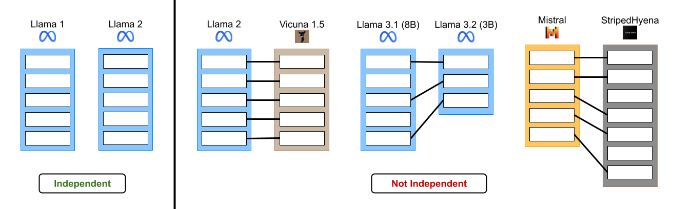
Figure 1: Given the weights of two language models, what relationships can we derive? They could be two models trained from scratch (left). Or, one model could be derived from the other: the dependent model could be a fine-tune, a pruned model, or a partially pruned model (right). We present tests to identify such relationships.

A solution to this independence testing problem would enable independent auditors to track provenance of open-weight models. This is pertinent because while open-weight models enable broader access and customization, they also pose potential risks for misuse as they cannot be easily monitored or moderated (kapoor2024openmodels). Model developers would also gain an enhanced ability to protect their intellectual property (IP) (2024miquscandal; Peng2023dnnip) and enforce custom model licenses (dubey2024llama3herdmodels; deepseekai2024deepseekv3technicalreport).

We consider two settings of the independence testing problem (Table 1). In the constrained setting, we make assumptions on training and initialization (essentially, that the training algorithm is equivariant to permuting the hidden units of the random initialization) that enable us to obtain provably valid p-values. The main idea is that under these assumptions we can cheaply simulate many exchangeable copies of each model’s weights and compare the value of some test statistic (e.g., cosine similarity of model weights) on each of these copies with the original model pair. The assumptions generally hold in practice but preclude robustness to adversarial evasion attacks and architectural changes.

For the constrained setting, we evaluate various test statistics on 21 models of the Llama 2 architecture (touvron2023llama2openfoundation), including 12 fine-tunes of Llama 2 and nine independently trained models, obtaining extremely small p-values for all 69 non-independent model pairs. Notably, our tests retain significant (small) p-values over different fine-tuning methods (e.g., different optimizers) and on models fine-tuned for many tokens from the base model such as Llemma (azerbayev2024llemmaopenlanguagemodel), which was fine-tuned on an additional 750B tokens from Llama 2 (37.5% of the Llama 2 training budget). We are also able to confirm that the leaked Miqu-70B model from Mistral is derived from Llama 2-70B.

Next, we consider the unconstrained setting. While the constrained setting is useful for studying the existing ecosystem of open-weight models, simple modifications to model weights and architecture such as permuting hidden units can violate the assumptions of the constrained setting if an adversary applies them after fine-tuning a model. We address this limitation in the unconstrained setting, wherein we do not make any assumptions on training. Though we are not able to obtain provably exact p-values in the unconstrained setting, we derive a test whose output empirically behaves like a p-value and reliably distinguishes non-independent models from independent models. In particular, we first align the hidden units of two models—which may each have different activation types and hidden dimensions—and then compute some measure of similarity between the aligned models. Because of the alignment step, the test is robust to changes in model architecture and various adversarial evasion attacks (including those that break prior work). Moreover, it can localize the dependence: we can identify specific components or weights that are not independent between two models, even when they have different architectures.

constrained setting	unconstrained setting
gives exact p-values	does not give exact p-values
not robust to permutation	robust to permutations and other adversarial transformations
only applies to models of fixed shared architecture	works for models of different architectures and gives localized testing of shared weights

Table 1: Features of the constrained versus unconstrained problem settings.

In the unconstrained setting, we evaluate our test on 141 independent model pairs and find that its output empirically behaves like a p-value in the sense that it is close to uniformly distributed in $(0,1]$ over these pairs. In contrast, it is almost zero for all dependent pairs we test (including those for which we simulate a somewhat strong adversary by retraining entire layers from scratch). We also employ our test to identify pruned model pairs, which occur when a model is compressed through dimension reduction techniques, such as reducing the number of layers or decreasing the hidden dimension by retaining select activations and weights; for example, we identified the precise layers of Llama 3.1-8B from which each of the layers of Llama 3.2-3B and Llama 3.2-1B derive.

We defer a full discussion of related work to Section LABEL:sec:related-work. The work most closely related to ours is due to zeng2024humanreadablefingerprintlargelanguage, who develop various tests to determine whether one model is independent of another by computing the cosine similarity of the products of certain weight matrices in both models. They show that their tests are robust to simple adversarial transformations of model weights that preserve model output; however, we detail in Appendix LABEL:app:breakhuref other transformations to perturb dependent models that evade detection by their tests, but not by our unconstrained setting tests. Additionally, unlike zeng2024humanreadablefingerprintlargelanguage, in the constrained setting we obtain exact p-values from our tests.

2 Methods

2.1 Problem formulation

Let $f:\Theta\times\mathcal{X}\to\mathcal{Y}$ denote a model mapping parameters $\theta\in\Theta$ and an input $X\in\mathcal{X}$ to an output $f(X;\theta)\in\mathcal{Y}$. We represent a model training or fine-tuning process as a learning algorithm $A:\Theta\to\Theta$ that takes as input a set of initial parameters corresponding to either a random initialization or, in the case of fine-tuning, base model parameters. Specifically, $A$ includes the choice of training data, ordering of minibatches, and all other design decisions and even the randomness used during training—everything other than the initial model weights.

Given two models $\theta_{1},\theta_{2}\sim P$ for some joint distribution $P\in\mathcal{P}(\Theta_{1}\times\Theta_{2})$, our goal is to test the null hypothesis

$$H_{0}:\theta_{1}\perp\theta_{2},$$ (1)

where $\perp$ denotes independence of two random variables. One example of a case where $\theta_{1}$ and $\theta_{2}$ might not be independent is if $\theta_{2}$ is fine-tuned from $\theta_{1}$, i.e. $\Theta_{1}=\Theta_{2}$ (meaning the two models share the same architecture) and $\theta_{2}=A(\theta_{1})$ for some learning algorithm $A$. We treat learning algorithms as deterministic functions. Thus for $\theta_{1}=A_{1}(\theta_{1}^{0})$ and $\theta_{2}=A_{2}(\theta_{2}^{0})$, then $\theta_{1}^{0}\perp\theta_{2}^{0}$, i.e., the two models having independent random initializations, implies our null hypothesis.

Deep learning models are often nested in nature. For example, Transformer models contain self-attention layers and multilayer perceptron (MLP) layers as submodels. We formalize the notion of a model containing another via the following definition of a submodel. We consider a projection operator that capture the subset of the full model’s parameters that are relevant to the submodel.

Definition 1.

A model $f:\mathcal{X}\times\Theta\to\mathcal{Y}$ contains a submodel $g:\mathcal{X}^{\prime}\times\Theta^{\prime}\to\mathcal{Y}^{\prime}$ if there exists a projection operator $\textup{proj}:\Theta\to\Theta^{\prime}$ such that for all $\theta\in\Theta$ we have

$$f(x;\theta)=f_{\textup{out}}(g(f_{\textup{in}}(x);\textup{proj}(\theta)))$$

for some functions $f_{\textup{in}}:\mathcal{X}\to\mathcal{X}^{\prime}$ and $f_{\textup{out}}:\mathcal{Y}^{\prime}\to\mathcal{Y}$ (which may depend on $\theta$).

Many of our experiments will specifically involve Transformer models containing MLP layers with Gated Linear Unit (GLU) activations, which are widely used among language models. We will thus specifically define this type of MLP using the following example.

Example 1 (): (GLU MLP) Let $G,U\in\mathbb{R}^{h\times d}$ and $D\in\mathbb{R}^{d\times h}$. Let $\sigma:\mathbb{R}\to\mathbb{R}$ be an element-wise activation function. For $x\in\mathbb{R}^{d}$ and $\theta=(G,U,D)\in\Theta_{\textup{mlp}}^{h}$, let $f_{\textup{mlp}}(x;\theta):=D(\sigma(Gx)\odot(Ux))$. Also, for $X\in\mathbb{R}^{s\times d}$ let $f_{\textup{mlp}}(X;\theta)\in\mathbb{R}^{s\times d}$ denote the result of broadcasting $f_{\textup{mlp}}$ over the rows of $X$. $\Diamond$

In addition to the basic independence testing problem above, we also consider the problem of localized testing: testing whether various pairs of submodels among two overall models are independent or not. A prototypical example of a localized testing problem is identifying which layers of a larger model (e.g., Llama 3.1-8B) were used to initialize a smaller model (e.g., Llama 3.2-3B) (in this case, we treat the layers as different submodels).

2.2 Constrained Setting

2.2.1 Testing Framework

Algorithm 1 (PERMTEST) encapsulates our framework for computing p-values against the null hypothesis in the constrained setting, wherein we simulate $T$ exchangeable copies of the first model $\theta_{1}$ by applying transformations to its weights. The exchangeability of these copies holds under some assumptions on the learning algorithm and random initialization that produced the original model. We capture these assumptions in the following definitions; together, they define the constrained setting.

Input: Model weights $\theta_{1},\theta_{2}$

Parameters : test statistic $\phi$; discrete transformation class $\Pi$; sample size $T$

Output: p-value $\hat{p}\in(0,1]$

1 $\mathtt{n\_ties}\leftarrow 0$

2 for $t\in 1,\dots,T$ do

3    $\pi_{t}\sim\textup{Unif}(\Pi)$

4    $\phi_{t}\leftarrow\phi(\pi_{t}(\theta_{1}),\theta_{2})$

5    $\mathtt{n\_ties}\leftarrow\mathtt{n\_ties}+\textbf{1}\{\phi_{t}=\phi(\theta_{1},\theta_{2})\}$

6   

$\xi\sim\textup{Unif}\left(\{0,...,\mathtt{n\_ties}\}\right)$ // break ties randomly

7 $\hat{p}\leftarrow\frac{1}{T+1}(1+\xi+\sum_{t=1}^{T}\textbf{1}\{\phi_{t}<\phi(\theta_{1},\theta_{2})\})$

return $1-\hat{p}$

Algorithm 1 Test for computing p-values (PERMTEST)

Definition 2 ($\Pi$-invariance).

Let $\Pi\subset\Theta\to\Theta$. A distribution $P\in\mathcal{P}(\Theta)$ is $\Pi$-invariant if for $\theta\sim P$ and any $\pi\in\Pi$, the parameters $\theta$ and $\pi(\theta)$ are identically distributed.

Definition 3 ($\Pi$-equivariance).

Let $\Pi\subset\Theta\to\Theta$, $\pi\in\Pi$, and $\theta^{0}\in\Theta$. A learning algorithm $A$ is $\Pi$-equivariant if and only if $\pi(A(\theta^{0}))=A(\pi(\theta^{0}))$.

The main idea underlying PERMTEST is that so long as $\theta_{1}=A(\theta_{1}^{0})$ and $\theta_{1}^{0}\sim P$ for some $\Pi$-equivariant learning algorithm $A$ and $\Pi$-invariant distribution $P$, we can simulate $T$ exchangeable (but not independent) copies $\{\pi_{t}(\theta_{1})\}_{t=1}^{T}$ of $\theta_{1}$ by sampling $\pi_{t}\overset{\text{i.i.d.}}{\sim}\textup{Unif}(\Pi)$. This allows us to efficiently compute an exact p-value without actually repeating the training process of $\theta_{1}$. In effect, Definitions 2 and 3 imply that $\pi$ commutes with $A$—i.e., $\pi(A(\theta_{1}^{0}))=A(\pi(\theta_{1}^{0}))$. Under exchangeability, the p-value output by PERMTEST will be uniformly distributed over $\{(i+1)/(T+1)\}_{i=0}^{T}$.

Standard initialization schemes for feedforward networks exhibit symmetry over their hidden units. This symmetry means that permuting hidden units represents one class of transformations under which any such initialization remains invariant. Moreover, the gradient of the model’s output with respect to the hidden units is permutation equivariant; thus, any learning algorithm whose update rule is itself a permutation equivariant function of gradients (e.g., SGD, Adam, etc.) satisfies Definition 3 with respect to these transformations. An example of a learning algorithm that is not permutation equivariant is one that uses different learning rates for each hidden unit depending on the index of the hidden unit.

Example 2 (Permuting hidden units): Let $\theta=(G,U,D)\in\Theta_{\textup{mlp}}^{h}$ parameterize a GLU MLP. Recall $f_{\textup{mlp}}(x;\theta):=D(\sigma(Gx)\odot(Ux))$ for some element-wise activation function $\sigma:\mathbb{R}\to\mathbb{R}$. Abusing notation, let $\Pi$ be the set of $h\times h$ permutation matrices such that for $\pi\in\Pi$ we define $\pi(\theta)=(\pi G,\pi U,D\pi^{T})$ (permuting the rows of $G,U$ and the columns of $D$). Observe $f_{\textup{mlp}}(x;\theta)=f_{\textup{mlp}}(x;\pi(\theta))$ and $\pi(\nabla_{\theta}f_{\textup{mlp}}(x;\theta))=\nabla_{\pi(\theta)}f(x;\pi(\theta))$ for all inputs $x$. $\Diamond$

The assumptions we make in the constrained setting suffice for PERMTEST to produce a valid $p$-value, as we show in the following theorem. Importantly, the result of the theorem holds (under the null hypothesis) without any assumptions on $\theta_{2}$. Therefore, a model developer of $\theta_{1}$ testing other models with our methods can have confidence in the validity of our test without trusting the provider of $\theta_{2}$. Of course, if $\theta_{2}$ does not satisfy the equivariance assumption on training (as in the unconstrained setting), then PERMTEST is unlikely to produce a low p-value even in cases where $\theta_{1}$ and $\theta_{2}$ are not independent (e.g. if an adversary finetunes $\theta_{2}$ from $\theta_{1}$ but then afterwards randomly permutes its hidden units).

Theorem 1.

Let $\phi:\Theta\times\Theta\to\mathbb{R}$ be a test statistic and $\Pi\subset\Theta\to\Theta$ be finite. Let $A:\Theta\to\Theta$ be $\Pi$-equivariant and let $P\in\mathcal{P}(\Theta)$ be $\Pi$-invariant. For $\theta_{1}^{0}\sim P$, let $\theta_{1}=A(\theta_{1}^{0})$. Let $\theta_{2}\in\Theta$ be independent of $\theta_{1}$. Then $\widehat{p}=\hyperref@@ii[algorithm:permtest]{\mathtt{PERMTEST}}(\theta_{1},\theta_{2})$ is uniformly distributed on $\{\frac{i+1}{T+1}\}_{i=0}^{T}$.

Proof.

We assume $\Pi$ is finite so that $\textup{Unif}(\Pi)$ is well-defined. From our assumptions on $A$ and $P$ and the fact that $\{\pi_{t}\}_{t=1}^{T}$ are independently drawn, it follows that the collection $\{\pi_{t}(\theta_{1})\}_{t=1}^{T}$ comprises $T$ exchangeable copies of $\theta_{1}$. The independence of $\theta_{1}$ and $\theta_{2}$ thus implies $\{(\pi_{t}(\theta_{1}),\theta_{2})\}_{t=1}^{T}$ comprises $T$ exchangeable copies of $(\theta_{1},\theta_{2})$. Because we break ties randomly, by symmetry it follows that $\phi(\theta_{1},\theta_{2})$ will have uniform rank among $\{\phi_{t}\}_{t=1}^{T}$. ∎

One notable (non-contrived) category of deep learning algorithms that are not permutation equivariant are those that employ dropout masks to hidden units during training. In our framework, the dropout masks are specified in the deterministic learning algorithm $A$. Once we fix a specific setting of mask values in $A$, this algorithm will not be permutation equivariant unless the individual dropout masks are all permutation invariant (which is highly unlikely). For completeness, we generalize the result of Theorem 1 to apply to randomized learning algorithms that satisfy a notion of equivariance in distribution (which includes algorithms that use dropout) in Appendix LABEL:sec:randomized-alg. However, throughout the main text we will continue to treat learning algorithms as deterministic for the sake of simplicity, and also since dropout typically is no longer used in training language models (chowdhery2022palmscalinglanguagemodeling).

2.2.2 Test Statistics

We have shown PERMTEST produces a valid p-value regardless of the test statistic $\phi$ we use. The sole objective then in designing a test statistic is to achieve high statistical power: we would like $\widehat{p}=\hyperref@@ii[algorithm:permtest]{\mathtt{PERMTEST}}(\theta_{1},\theta_{2})$ to be small when $\theta_{1}$ and $\theta_{2}$ are not independent. The test statistics we introduce in this section apply to any model pair sharing the same architecture.

Prior work (xu2024instructionalfingerprintinglargelanguage) proposed testing whether two models are independent or not based on the $\ell_{2}$ distance between their weights, summed over layers. Specifically for a model with $L$ layers parameterized by $\Theta=\Theta_{1}\times...\times\Theta_{L}$, with $\theta_{1}=(\theta_{1}^{(\ell)})_{\ell=1}^{L}$ and $\theta_{2}=(\theta_{2}^{(\ell)})_{\ell=1}^{L}$, let $\phi_{\ell_{2}}(\theta_{1},\theta_{2}):=-\sum_{i=1}^{L}\ell_{2}(\theta_{1}^{(i)},\theta_{2}^{(i)})$. We can obtain p-values from $\phi_{\ell_{2}}$ by using it within PERMTEST. However, a major limitation is that in order to obtain a p-value less than $1/(T+1)$ we must recompute $\phi_{\ell_{2}}$ at least $T$ times; the effective statistical power of our test using $\phi_{\ell_{2}}$ is therefore bottlenecked by computation.

To address this limitation, we propose a family of test statistics whose distribution under the null is identical for any model pair. Consider $m,n\in\mathbb{N}$ and some function $M:\Theta\to\mathbb{R}^{n\times m}$ that maps model weights to a matrix, such as returning a specific layer’s weight matrix. The proposed test statistics all share the following general form based on Algorithm LABEL:alg:speartest (MATCH) for varying $M$:

(2)