Towards Practical First-Order Model Counting

Abstract

First-order model counting (FOMC) is the problem of counting the number of models of a sentence in first-order logic. Since lifted inference techniques rely on reductions to variants of FOMC, the design of scalable methods for FOMC has attracted attention from both theoreticians and practitioners over the past decade. Recently, a new approach based on first-order knowledge compilation was proposed. This approach, called Crane, instead of simply providing the final count, generates definitions of (possibly recursive) functions that can be evaluated with different arguments to compute the model count for any domain size. However, this approach is not fully automated, as it requires manual evaluation of the constructed functions. The primary contribution of this work is a fully automated compilation algorithm, called Gantry, which transforms the function definitions into C++ code equipped with arbitrary-precision arithmetic. These additions allow the new FOMC algorithm to scale to domain sizes over $500,000$ times larger than the current state of the art, as demonstrated through experimental results.

1 Introduction

First-order model counting (FOMC) is the task of determining the number of models for a sentence in first-order logic over a specified domain. The weighted variant, WFOMC, computes the total weight of these models, linking logical reasoning with probabilistic frameworks [30]. It builds upon earlier efforts in weighted model counting for propositional logic [4] and broader attempts to bridge logic and probability [13, 15, 19]. WFOMC is central to lifted inference, which enhances the efficiency of probabilistic calculations by exploiting symmetries [10]. Lifted inference continues to advance, with applications extending to constraint satisfaction problems [24] and probabilistic answer set programming [1]. Moreover, WFOMC has proven effective at reasoning over probabilistic databases [8] and probabilistic logic programs [17]. FOMC algorithms have also facilitated breakthroughs in discovering integer sequences [21] and developing recurrence relations for these sequences [6]. Recently, these algorithms have been extended to perform sampling tasks [31].

The complexity of FOMC is generally measured by data complexity, with a sentence classified as liftable if it admits a polynomial-time solution relative to the domain size [9]. While all sentences with up to two variables are known to be liftable [27, 29], Beame et al. [3] demonstrated that liftability does not extend to all sentences, identifying an unliftable sentence with three variables. Recent work has extended the liftable fragment with additional axioms [22, 26] and counting quantifiers [11], expanding our understanding of liftability.

FOMC algorithms are diverse, with approaches ranging from first-order knowledge compilation (FOKC) to cell enumeration [25], local search [14], and Monte Carlo sampling [7]. (See Appendix˜A for a more detailed comparison of the state-of-the-art FOMC algorithms.) FOKC-based algorithms are particularly prominent, transforming sentences into structured representations such as circuits or graphs. Even when multiple algorithms can solve the same instance, FOKC algorithms are known to find polynomial-time solutions where the polynomial has a lower degree than other approaches [6]. The recently developed ability of a FOKC algorithm to formulate solutions in terms of recursive functions [6] is also noteworthy since the only other proposed alternative is to guess recursive relations [2]. Notable examples of FOKC algorithms include ForcLift [30] and its extension Crane [6].

The Crane algorithm marked a significant step forward, expanding the range of sentences handled by FOMC algorithms. However, it had notable limitations: it required manual evaluation of function definitions to compute model counts and introduced recursive functions without proper base cases, making it more difficult to use. To address these shortcomings, we present Gantry, a fully automated FOMC algorithm that overcomes the constraints of its predecessor. Gantry can handle domain sizes over $500,000$ times larger than those of previous algorithms and simplifies the user experience by automatically managing base cases and compiling function definitions into efficient C++ programs.

The paper is structured as follows. Section˜2 covers the necessary preliminaries, including notation, terminology, and background information about (W)FOMC and FOKC. Section˜3 describes all aspects of Gantry:

• its overall structure and interactions with Crane,

• how we identify a sufficient set of base cases for a recursive function,

• how we construct the sentence that describes each base case, and

• how we compile function definitions into a C++ program with caching mechanisms that ensure efficiency.

Then, Section˜4 presents our experimental results, demonstrating Gantry’s performance compared to other FOMC algorithms. Finally, Section˜5 concludes the paper by discussing promising avenues for future work.

2 Preliminaries

We begin this section by describing some notation that we will use throughout the paper. Then, in Sections˜2.1 and 2.2, we introduce the basic terminology of first-order logic and formally define (W)FOMC. Section˜2.3 outlines the principles of FOKC, particularly in the context of Crane. Finally, in Section˜2.4, we introduce the algebraic terminology used to describe the output of Crane, i.e., functions and equations that define them.

Notation

We use $\mathbb{N}_{0}$ to represent the set of non-negative integers. In both algebra and logic, we write $S\sigma$ to denote the application of a substitution $\sigma$ to an expression $S$, where $\sigma=[x_{1}\mapsto y_{1},x_{2}\mapsto y_{2},\dots,x_{n}\mapsto y_{n}]$ signifies the replacement of all instances of $x_{i}$ with $y_{i}$ for all $i=1,\dots,n$. Additionally, for any variable $n$ and $a,b\in\mathbb{N}_{0}$, let $[a\leq n\leq b]\coloneqq\begin{cases}1&\text{if $a\leq n\leq b$}\\ 0&\text{otherwise}\end{cases}$.

2.1 First-Order Logic

This section reviews the basic concepts of first-order logic used in FOKC algorithms. We focus specifically on the format used internally by ForcLift and its descendants. See Section˜2.3.1 for a brief overview of how Gantry transforms an arbitrary sentence in first-order logic into this internal format.

A term can be either a variable or a constant. An atom can be either $P(t_{1},\dots,t_{m})$ (i.e., $P(\mathbf{t})$) for some predicate $P$ and terms $t_{1},\dots,t_{m}$, or $x=y$ for some terms $x$ and $y$. The arity of a predicate is the number of arguments it takes, i.e., $m$ in the case of the predicate $P$ mentioned above. We write $P/m$ to denote a predicate along with its arity. A literal can be either an atom (i.e., a positive literal) or its negation (i.e., a negative literal). An atom containing no variables, only constants, is called ground. A clause is of the form $\forall x_{1}\in\Delta_{1}\text{. }\forall x_{2}\in\Delta_{2}\dots\text{ }\forall x_{n}\in\Delta_{n}\text{. }\phi(x_{1},x_{2},\dots,x_{n})$, where $\phi$ is a disjunction of literals that contain only the variables $x_{1},\dots,x_{n}$ (and any constants). We say that a clause is a (positive) unit clause if there is only one literal with a predicate, and it is a positive literal. Finally, a sentence is a conjunction of clauses. Throughout the paper, we will use set-theoretic notation, interpreting a sentence as a set of clauses and a clause as a set of literals.

Conforming to previous work [30], the definition of a clause includes universal quantifiers for all its variables. While it is possible to rewrite the entire sentence with all quantifiers at the front, the format we describe has proven convenient for practical use.

2.2 First-Order Model Counting

In this section, we will formally define FOMC and its weighted variant. Although this work focuses on FOMC, computing the FOMC using Gantry requires using WFOMC for sentences with existential quantifiers. For such sentences, preprocessing (described in Section˜2.3.1) introduces predicates with non-unary weights that must be accounted for to compute the correct model count.

Definition 2.1 (Structure, model).

Let $\phi$ be a sentence. For each predicate $P/n$ in $\phi$, let ${(\Delta_{i}^{P})}_{i=1}^{n}$ be a list of the corresponding domains. Let $\sigma$ be a map from the domains of $\phi$ to their interpretations as finite sets, ensuring the sets are pairwise disjoint and contain the corresponding constants from $\phi$. A structure of $\phi$ is a set $M$ of ground literals defined by adding to $M$ either $P(\mathbf{t})$ or $\neg P(\mathbf{t})$ for every predicate $P/n$ in $\phi$ and every $n$-tuple $\mathbf{t}\in\prod_{i=1}^{n}\sigma(\Delta_{i}^{P})$. A structure is a model if it makes $\phi$ valid.

Example 2.2 (Counting bijections).

Let us consider the following sentence (previously examined by Dilkas and Belle [6]) that defines predicate $P$ as a bijection between two domains $\Gamma$ and $\Delta$:

$$\begin{gathered}(\forall x\in\Gamma\text{. }\exists y\in\Delta\text{. }P(x,y))\land{}\\ (\forall y\in\Delta\text{. }\exists x\in\Gamma\text{. }P(x,y))\land{}\\ (\forall x\in\Gamma\text{. }\forall y,z\in\Delta\text{. }P(x,y)\land P(x,z)\Rightarrow y=z)\land{}\\ (\forall x,z\in\Gamma\text{. }\forall y\in\Delta\text{. }P(x,y)\land P(z,y)\Rightarrow x=z).\end{gathered}$$ (1)

Let $\sigma$ be defined as $\sigma(\Gamma)\coloneqq\{\,1,2\,\}$ and $\sigma(\Delta)\coloneqq\{\,a,b\,\}$. Equation˜1 has two models:

$$\{\,P(1,a),P(2,b),\neg P(1,b),\neg P(2,a)\,\}\qquad\text{and}\qquad\{\,P(1,b),P(2,a),\neg P(1,a),\neg P(2,b)\,\}.$$

The distinctness of domains is significant in two respects. First, in terms of expressiveness, a clause such as $\forall x\in\Delta\text{. }P(x,x)$ is valid if predicate $P$ operates over two copies of the same domain and invalid otherwise. Second, having more distinct domains makes the problem more decomposable for the FOKC algorithm. With distinct domains, the algorithm can make assumptions or deductions about, e.g., the first domain of predicate $P$ without worrying how (or if) they apply to the second domain.

Definition 2.3 (WFOMC instance).

A WFOMC instance comprises:

• a sentence $\phi$,

• two (rational) weights $w^{+}(P)$ and $w^{-}(P)$ assigned to each predicate $P$ in $\phi$, and

• $\sigma$ as described in Definition˜2.1.

Unless specified otherwise, we assume all weights are equal to 1.

Definition 2.4 (WFOMC [30]).

Given a WFOMC instance $(\phi,w^{+},w^{-},\sigma)$ as in Definition˜2.3, the (symmetric) weighted first-order model count (WFOMC) of $\phi$ is

$$\sum_{M\models\phi}\prod_{P(\mathbf{t})\in M}w^{+}(P)\prod_{\neg P(\mathbf{t})\in M}w^{-}(P),$$ (2)

where the sum is over all models of $\phi$.

2.3 Crane and First-Order Knowledge Compilation

As our work builds on Crane, in this section, we will briefly outline the steps Crane goes through to compile a sentence into a set of function definitions. We divide the inner workings of the algorithm into two stages: preprocessing and compilation.

2.3.1 Preprocessing

This stage transforms an arbitrary sentence into the format described in Section˜2.1, primarily by eliminating existential quantifiers. For example, the first conjunct of Equation˜1, i.e.,

$$\forall x\in\Gamma\text{. }\exists y\in\Delta\text{. }P(x,y)$$ (3)

is transformed into

$$(\forall x\in\Gamma\text{. } Z(x))\land{}$$ (4)

$$(\forall x\in\Gamma\text{. }\forall y\in\Delta\text{. } Z(x)\lor\neg P(x,y))\land{}$$

$$(\forall x\in\Gamma\text{. } S(x)\lor Z(x))\land{}$$

$$(\forall x\in\Gamma\text{. }\forall y\in\Delta\text{. } S(x)\lor\neg P(x,y)),$$

where $Z/1$ and $S/1$ are two new predicates with $w^{-}(S)=-1$. One can verify that the WFOMC of Equations˜3 and 4 is the same.

2.3.2 Compilation

After preprocessing, Crane compiles the sentence into the triple $(\mathcal{E},\mathcal{F},\mathcal{D})$, where $\mathcal{E}$ is the set of equations, and $\mathcal{F}$ and $\mathcal{D}$ are auxiliary maps. $\mathcal{F}$ maps function names to sentences. $\mathcal{D}$ maps function names and argument indices to domains. $\mathcal{E}$ can contain any number of functions, one of which (which we will always denote as $f$) represents the solution to the FOMC problem. Computing the FOMC for specific domain sizes involves invoking $f$ with those sizes as inputs. $\mathcal{D}$ records this correspondence between function arguments and domains.

Example 2.5.

Crane compiles Equation˜1 for bijection counting into

$$\mathcal{E} =\left\{\,\begin{aligned} f(m,n)&=\sum_{l=0}^{n}\binom{n}{l}{(-1)}^{n-l}g(l,m),\\ g(l,m)&=\sum_{k=0}^{m}[0\leq k\leq 1]\binom{m}{k}g(l-1,m-k)\end{aligned}\,\right\};$$

$$\mathcal{D} =\{\,(f,1)\mapsto\Gamma,(f,2)\mapsto\Delta,(g,1)\mapsto\Delta^{\top},(g,2)\mapsto\Gamma\,\},$$

where $\Delta^{\top}$ is a newly introduced domain. (We omit the definition of $\mathcal{F}$ as the sentences can become quite verbose.) To compute the number of bijections between two sets of cardinality 3, one would evaluate $f(3,3)$; however, the definition of $g$ is incomplete: $g$ is a recursive function presented without any base cases. $\mathcal{D}$ encodes that in $f(m,n)$, $m$ and $n$ represent $|\Gamma|$ and $|\Delta|$, respectively. Similarly, in $g(l,m)$, $l$ represents $|\Delta^{\top}|$, and $m$ represents $|\Gamma|$.

Compilation is performed primarily by applying (compilation) rules to sentences. Crane has two modes depending on the selection process for compilation rules when multiple alternatives are available. The first option is to use greedy search: there is a list of rules, and the first applicable rule is the one that gets used, disregarding all the others. The second option is to use a combination of greedy and breadth-first search (BFS). In this approach, we classify each compilation rule as greedy or non-greedy. Greedy rules are applied as soon as possible at any stage of the compilation process, while BFS is executed over all applicable non-greedy rules, identifying the solution that necessitates the smallest number of non-greedy rules.

2.4 Algebra

In this paper, we use both logical and algebraic constructs. While the rest of Section˜2 focused on the former, this section describes the latter. We write $\mathtt{expr}{}$ for an arbitrary algebraic expression. In the context of algebra, a constant is a non-negative integer. Likewise, a variable can either be a parameter of a function or a variable introduced through summation, such as $i$ in the expression $\sum_{i=1}^{n}\mathtt{expr}$. A function call is $f(x_{1},\dots,x_{n})$ (or $f(\mathbf{x})$ for short), where $f$ is an $n$-ary function, and each $x_{i}$ is an algebraic expression consisting of variables and constants. A (function) signature is a function call that contains only variables. Given two function calls, $f(\mathbf{x})$ and $f(\mathbf{y})$, we say that $f(\mathbf{y})$ matches $f(\mathbf{x})$ if $x_{i}=y_{i}$ whenever $x_{i},y_{i}\in\mathbb{N}_{0}$. An equation is $f(\mathbf{x})=\mathtt{expr}{}$, where $f(\mathbf{x})$ is a function call.

Definition 2.6 (Base case).

Let $f(\mathbf{x})$ be a function call where each $x_{i}$ is either a constant or a variable. Then the function call $f(\mathbf{y})$ is a base case of $f(\mathbf{x})$ if $f(\mathbf{y})=f(\mathbf{x})\sigma$, where $\sigma$ is a substitution that replaces one or more variable $x_{i}$’s with a constant while leaving constants unchanged.

Example 2.7.

In the equation $f(m,n)=f(m-1,n)+nf(m-1,n-1)$, the only constant is $1$, and the variables are $m$ and $n$. The equation contains three function calls: one on the left-hand side (LHS) and two on the right-hand side (RHS). The function call on the LHS is a signature. Function calls such as $f(4,n)$, $f(m,0)$, and $f(8,1)$ are all considered base cases of $f(m,n)$ (only some of which are useful).

3 Technical Contributions

Figure 1: Using Gantry to compute the model count of a sentence $\phi$. First, Gantry compiles $\phi$ into a set of equations, which form the basis for creating a C++ program. Executing the program with different command line arguments calculates the model count of $\phi$ for various domain sizes. To accomplish this, the CompileWithBaseCases procedure employs Crane, algebraic simplification techniques (denoted as Simplify), and two other auxiliary procedures.

Figure˜1 provides an overview of Gantry’s workflow. We will briefly describe and motivate each procedure before going into more detail in the corresponding subsection.

CompileWithBaseCases (see Section˜3.1), the core procedure of Gantry, is responsible for completing the function definitions produced by Crane with the necessary base cases. To do so, it may recursively call itself (and Crane) on other sentences. We prove that the number of such recursive calls is upper bound by the number of domains.

Section˜3.1 also describes the Simplify procedure for algebraic simplification. It is crucial for simplifying, e.g., a sum of $n$ terms, only some of which are non-zero. More generally, the equations returned by Crane often benefit from easily detectable algebraic simplifications such as $0\cdot\text{anything}=0$ and $\text{anything}^{0}=1$.

FindBaseCases (described in Section˜3.2) inspects a set of equations to identify a sufficient set of base cases for a given set of equations. We prove that the returned set of base cases ensures that the evaluation of the resulting function definitions will never get stuck in an infinite loop.

Section˜3.3 introduces the Propagate procedure, which takes a sentence $\phi$, a domain $\Delta$, and $n\in\mathbb{N}_{0}$. It returns $\phi$ transformed under the assumption that $|\Delta|=n$, with $n$ new constants added and all variables quantified over $\Delta$ eliminated. For example, when computing a base case such as $f(0,y)$, Propagate will significantly simplify $\phi$ with the assumption that the domain associated with the first parameter of $f$ (i.e., $\mathcal{D}(f,1)$) is empty. CompileWithBaseCases(Propagate($\phi$, $\mathcal{D}(f,1)$, $0$)) will then return the equations for the base case $f(0,y)$.

Section˜3.4 describes a new smoothing procedure that ensures Propagate preserves the correct model count. Smoothing is a well-known technique in knowledge compilation algorithms for propositional model counting [5]. Although FOMC algorithms have used smoothing before [30], our setting requires a novel approach.

With the help of other procedures outlined above, CompileWithBaseCases returns a set of equations that fully cover the base cases of all recursive functions. While these equations can be intriguing and valuable in their own right, users of FOMC algorithms typically expect a numerical answer. Thus, Section˜3.5 describes how Gantry compiles these equations into a C++ program that one can execute with different command-line arguments to compute the model count for various combinations of domain sizes.

3.1 Completing the Definitions of Functions

Input: sentence $\phi$

Output: set $\mathcal{E}$ of equations

1 $(\mathcal{E},\mathcal{F},\mathcal{D})\leftarrow\textnormal{{{{Crane}}(}}\textnormal{\emph{$\phi$}}\textnormal{{)}}$;

2 $\mathcal{E}\leftarrow\textnormal{{Simplify(}}\textnormal{\emph{$\mathcal{E}$}}\textnormal{{)}}$;

3 foreach base case $f(\mathbf{x})\in\textnormal{{FindBaseCases(}}\textnormal{\emph{$\mathcal{E}$}}\textnormal{{)}}$ do

4    $\psi\leftarrow\mathcal{F}(f)$;

5    foreach index $i$ such that $x_{i}\in\mathbb{N}_{0}$ do $\psi\leftarrow\textnormal{{Propagate(}}\textnormal{\emph{$\psi$, $\mathcal{D}(f,i)$, $x_{i}$}}\textnormal{{)}}$;

6    $\mathcal{E}\leftarrow\mathcal{E}\cup\textnormal{{CompileWithBaseCases(}}\textnormal{\emph{$\psi$}}\textnormal{{)}}$;

7   

Algorithm 1 CompileWithBaseCases($\phi$)

Algorithm˜1 presents our overall approach for compiling a sentence into equations that include the necessary base cases. First, we use Crane to compile the sentence into three components: $\mathcal{E}$, $\mathcal{F}$, and $\mathcal{D}$ (as described in Section˜2.3.2). After some algebraic simplifications (described below), the algorithm passes $\mathcal{E}$ to the FindBaseCases procedure (see Section˜3.2). For each base case $f(\mathbf{x})$, we retrieve the sentence $\mathcal{F}(f)$ associated with the function name $f$ and simplify it using the Propagate procedure (explained in detail in Section˜3.3). We do this by iterating over all indices of $\mathbf{x}$, where $x_{i}$ is a constant, and using Propagate to simplify $\psi$ by assuming that domain $\mathcal{D}(f,i)$ has size $x_{i}$. Finally, on algorithm 1, CompileWithBaseCases recurses on these simplified sentences and adds the resulting base case equations to $\mathcal{E}$.

Simplify

The main responsibility of the Simplify procedure is to handle the algebraic pattern $\sum_{m=0}^{n}[a\leq m\leq b]f(m)$. Here, $n$ is a variable, $a$ and $b$ are constants, and $f$ is an expression that may depend on $m$. Simplify transforms this pattern into $f(a)+f(a+1)+\cdots+f(\min\{\,n,b\,\})$.

Example 3.1.

We return to the bijection-counting problem from Example˜2.2 and its initial solution described in Example˜2.5. Simplify transforms

$$g(l,m)=\sum_{k=0}^{m}[0\leq k\leq 1]\binom{m}{k}g(l-1,m-k)$$

into

$$g(l,m)=g(l-1,m)+mg(l-1,m-1).$$

Then FindBaseCases identifies two base cases: $g(0,m)$ and $g(l,0)$. In both cases, CompileWithBaseCases recurses on the sentence $\mathcal{F}(g)$ simplified by assuming that one of the domains is empty. In the first case, we recurse on the sentence $\forall x\in\Gamma\text{. }S(x)\lor\neg S(x)$, where $S$ is a predicate introduced by preprocessing with weights $w^{+}(S)=1$ and $w^{-}(S)=-1$. Hence, we obtain the base case $g(0,m)=0^{m}$. In the case of $g(l,0)$, Propagate($\psi$, $\Gamma$, $0$) returns an empty sentence, resulting in $g(l,0)=1$. While these base cases overlap when $l=m=0$, they remain consistent since $0^{0}=1$.

Generally, let $\phi$ be a sentence with two domains $\Gamma$ and $\Delta$, and let $n,m\in\mathbb{N}_{0}$. Then the FOMC of Propagate($\phi$, $\Delta$, $n$), assuming $|\Gamma|=m$, is the same as the FOMC of Propagate($\phi$, $\Gamma$, $m$), assuming $|\Delta|=n$.

Although CompileWithBaseCases starts with a call to Crane, the proposed algorithm is not merely a post-processing step for FOKC because Algorithm˜1 is recursive and can issue additional calls to Crane on various derived sentences. We conclude this section by bounding the recursion depth of the CompileWithBaseCases procedure, thereby also proving that the algorithm terminates.

Theorem 3.2.

Let $\phi$ be a sentence with $n$ domains. The maximum recursion depth of CompileWithBaseCases($\phi$) is then $n$.

The proof of this theorem relies on two observations regarding the algorithms presented in Sections˜3.2 and 3.3.

Each base case returned by FindBaseCases contains at least one constant (in line with Definition˜2.6).

For any sentence $\phi$, domain $\Delta$, and $n\in\mathbb{N}_{0}$, Propagate($\phi$, $\Delta$, $n$) returns a sentence with no variables quantified over $\Delta$.

Proof 3.3.

We proceed by induction on $n$. If $n=0$, then $\phi$ is essentially a propositional formula, and Crane compiles it into an equation of the form $f=\mathtt{expr}$ with no ‘function calls’. Suppose that—for all sentences with at most $n$ domains—CompileWithBaseCases terminates with a recursion depth of at most $n$. Let $\phi$ be a sentence with $n+1$ domains. By Section˜3.1, each base case on algorithm 1 of Algorithm˜1 has at least one constant. Therefore, by Section˜3.1, after algorithm 1, the sentence $\psi$ has at most $n$ domains. Thus, algorithm 1 terminates with a recursion depth of at most $n$ by the inductive hypothesis, completing the inductive proof.

3.2 Identifying a Sufficient Set of Base Cases

Input: set $\mathcal{E}$ of equations

Output: set $\mathcal{B}$ of base cases

1

2$\mathcal{B}\leftarrow\emptyset$;

3 foreach function call $f(\mathbf{y})$ on the RHS of an equation in $\mathcal{E}$ do

4    $\mathbf{x}\leftarrow\text{the parameters of $f$ in its definition}$;

5    foreach $y_{i}\in\mathbf{y}$ do

6       if $y_{i}\in\mathbb{N}_{0}$ then $\mathcal{B}\leftarrow\mathcal{B}\cup\{\,f(\mathbf{x})[x_{i}\mapsto y_{i}]\,\}$;

7       else if $y_{i}=x_{i}-c_{i}$ for some $c_{i}\in\mathbb{N}_{0}$ then

8          for $j\leftarrow 0$ to $c_{i}-1$ do $\mathcal{B}\leftarrow\mathcal{B}\cup\{\,f(\mathbf{x})[x_{i}\mapsto j]\,\}$;

9         

10      

11   

Algorithm 2 FindBaseCases($\mathcal{E}$)

Algorithm˜2 summarises the implementation of FindBaseCases. It considers two types of arguments when a function $f$ calls itself recursively: constants and arguments of the form $x_{i}-c_{i}$. When the argument is a constant $c_{i}$, algorithm 2 adds a base case with $c_{i}$ to the set of all base cases $\mathcal{B}$. In the second case, algorithm 2 adds a base case to $\mathcal{B}$ for each constant from $0$ to (but not including) $c_{i}$.

Example 3.4.

Consider the recursive function $g$ from Example˜2.5. FindBaseCases iterates over two function calls: $g(l-1,m)$ and $g(l-1,m-1)$. The former produces the base case $g(0,m)$, while the latter produces both $g(0,m)$ and $g(l,0)$.

In the rest of this section, we will show that the base cases identified by FindBaseCases are sufficient for the algorithm to terminate. Let $\mathcal{E}$ denote the equations returned by CompileWithBaseCases.

Theorem 3.5.

Given an $n$-ary function $f$ in $\mathcal{E}$ and $\mathbf{x}\in\mathbb{N}_{0}^{n}$, the evaluation of $f(\mathbf{x})$ terminates.

We prove Theorem˜3.5 using double induction. First, we apply induction to the number of functions in $\mathcal{E}$. Then, we use induction on the arity of the ‘last’ function in $\mathcal{E}$ according to a topological ordering. Before proving Theorem˜3.5, we make a few observations about this and previous [6, 30] work.

For each function $f$, there is precisely one equation $e\in\mathcal{E}$ with $f(\mathbf{x})$ on the LHS where all $x_{i}$’s are variables (i.e., $e$ is not a base case). We refer to $e$ as the definition of $f$.

There is a topological ordering ${(f_{i})}_{i}$ of all functions in $\mathcal{E}$ such that equations in $\mathcal{E}$ with $f_{i}$ on the LHS do not contain function calls to $f_{j}$ with $j>i$.

Section˜3.2 prevents mutual recursion and other cyclic scenarios.

For each equation $(f(\mathbf{x})=\mathtt{expr})\in\mathcal{E}$, the evaluation of $\mathtt{expr}$ terminates when provided with the values of all relevant function calls.

Corollary 3.6.

If $f$ is a non-recursive function with no function calls on the RHS of its definition, then the evaluation of any function call $f(\mathbf{x})$ terminates.

For each equation $(f(\mathbf{x})=\mathtt{expr}{})\in\mathcal{E}$, if $\mathbf{x}$ contains only constants, then $\mathtt{expr}{}$ cannot include any function calls to $f$.

Additionally, we introduce an assumption about the structure of recursion.

Assumption 3.7.

For each equation $(f(\mathbf{x})=\mathtt{expr})\in\mathcal{E}$, every recursive function call $f(\mathbf{y})\in\mathtt{expr}$ satisfies the following:

• each $y_{i}$ is either $x_{i}-c_{i}$ or $c_{i}$ for some constant $c_{i}$ and

• there exists $i$ such that $y_{i}=x_{i}-c_{i}$ for some $c_{i}>0$.

Finally, we assume a particular order of evaluation for function calls using the equations in $\mathcal{E}$; specifically, base cases precede the recursive definition.

Assumption 3.8.

When multiple equations in $\mathcal{E}$ match a function call $f(\mathbf{x})$, preference is given to the equation with the most constants on its LHS.

With the observations and assumptions mentioned above, we are ready to prove Theorem˜3.5. For readability, we divide the proof into several lemmas of increasing generality.

Lemma 3.9.

Assume that $\mathcal{E}$ consists of just one unary function called $f$. Then the evaluation of $f(x)$ terminates for any $x\in\mathbb{N}_{0}$.

Proof 3.10.

If $f(x)$ matches a base case, then its evaluation terminates by Corollaries˜3.6 and 3.2. If $f$ is not recursive, the evaluation of $f(x)$ also terminates by Corollary˜3.6.

Otherwise, let $f(y)$ be an arbitrary function call on the RHS of the definition of $f(x)$. If $y$ is a constant, then there is a base case for $f(y)$. Otherwise, let $y=x-c$ for some $c>0$. Then there exists $k\in\mathbb{N}_{0}$ such that $0\leq x-kc\leq c-1$. So, after $k$ iterations, the sequence of function calls $f(x),f(x-c),f(x-2c),\dots$ will match the base case $f(x\mod c)$.

Lemma 3.11.

Generalising Lemma˜3.9, let $\mathcal{E}$ be a set of equations for one $n$-ary function $f$ for some $n\geq 1$. The evaluation of $f(\mathbf{x})$ terminates for any $\mathbf{x}\in\mathbb{N}_{0}^{n}$.

Proof 3.12.

If $f$ is non-recursive, the evaluation of $f(\mathbf{x})$ terminates by previous arguments. We proceed by induction on $n$, with the base case of $n=1$ handled by Lemma˜3.9. Assume that $n>1$. Any base case of $f$ can be seen as a function of arity $n-1$ since one of the parameters is constant. Thus, the evaluation of any base case terminates by the inductive hypothesis. It remains to show that the evaluation of the recursive equation for $f$ terminates, but this follows from Section˜3.2.

Proof 3.13 (Proof of Theorem˜3.5).

We proceed by induction on the number of functions $n$. The base case of $n=1$ is handled by Lemma˜3.11. Let ${(f_{i})}_{i=1}^{n}$ be some topological ordering of these $n>1$ functions. If $f=f_{j}$ for $j<n$, then the evaluation of $f(\mathbf{x})$ terminates by the inductive hypothesis since $f_{j}$ cannot call $f_{n}$ by Section˜3.2. Using the inductive hypothesis that all function calls to $f_{j}$ (with $j<n$) terminate, the proof proceeds similarly to the proof of Lemma˜3.11.

3.3 Propagating Domain Size Assumptions

Input: sentence $\phi$, domain $\Delta$, $n\in\mathbb{N}_{0}$

Output: sentence $\phi^{\prime}$

1 $\phi^{\prime}\leftarrow\emptyset$;

2 if $n=0$ then

3    foreach clause $C\in\phi$ do

4       if $\Delta\not\in\operatorname{Doms}(C)$ then $\phi^{\prime}\leftarrow\phi^{\prime}\cup\{\,C\,\}$;

5       else

6          $C^{\prime}\leftarrow\{\,l\in C\mid\Delta\not\in\operatorname{Doms}(l)\,\}$;

7          if $C^{\prime}\neq\emptyset$ then

8             $l\leftarrow\text{an arbitrary literal in }C^{\prime}$;

9             $\phi^{\prime}\leftarrow\phi^{\prime}\cup\{\,C^{\prime}\cup\{\,\neg l\,\}\,\}$;

10            

11         

12      

13   

14 else

15    $D\leftarrow\text{a set of $n$ new constants in $\Delta$}$;

16    foreach clause $C\in\phi$ do

17       ${(x_{i})}_{i=1}^{m}\leftarrow\text{the variables in $C$ with domain $\Delta$}$;

18       if $m=0$ then $\phi^{\prime}\leftarrow\phi^{\prime}\cup\{\,C\,\}$;

19       else $\phi^{\prime}\leftarrow\phi^{\prime}\cup\{\,C[x_{1}\mapsto c_{1},\dots,x_{m}\mapsto c_{m}]\mid{(c_{i})}_{i=1}^{m}\in D^{m}\,\}$;

20      

21   

Algorithm 3 Propagate($\phi$, $\Delta$, $n$)

Algorithm˜3, called Propagate, modifies the sentence $\phi$ based on the assumption that $|\Delta|=n$. When $n=0$, some clauses become vacuously satisfied and can be removed. When $n>0$, partial grounding replaces all variables with domain $\Delta$ with constants. (None of the sentences examined in this work had $n>1$.) Algorithm˜3 handles these two cases separately. For a literal or clause $C$, we write the set of corresponding domains as $\operatorname{Doms}(C)$. In the case of $n=0$, there are three types of clauses to consider:

1. those that do not mention $\Delta$,

2. those in which every literal contains variables quantified over $\Delta$ and

3. those with some literals containing such variables and some without.

We transfer clauses of Item˜1 to the new sentence $\phi^{\prime}$ without any changes. For clauses of Item˜2, $C^{\prime}$ is empty, so these clauses are filtered out. As for clauses of Item˜3, lines 3–3 perform a new kind of smoothing, the explanation of which we defer to Section˜3.4.

In the case of $n>0$, $n$ new constants are introduced. Let $C$ be an arbitrary clause in $\phi$, and let $m\in\mathbb{N}_{0}$ be the number of variables in $C$ quantified over $\Delta$. If $m=0$, $C$ is added directly to $\phi^{\prime}$. Otherwise, a clause is added to $\phi^{\prime}$ for every possible combination of replacing the $m$ variables in $C$ with the $n$ new constants.

Example 3.14.

Let $C\coloneqq\forall x\in\Gamma\text{. }\forall y,z\in\Delta\text{. }\neg P(x,y)\lor\neg P(x,z)\lor y=z$. Then $\operatorname{Doms}(C)=\operatorname{Doms}(\neg P(x,y))=\operatorname{Doms}(\neg P(x,z))=\{\,\Gamma,\Delta\,\}$, and $\operatorname{Doms}(y=z)=\{\,\Delta\,\}$. A call to Propagate($\{\,C\,\}$, $\Delta$, $3$) would result in the following sentence with nine clauses:

$$(\forall x\in\Gamma\text{. }\neg P(x,c_{1})\lor \neg P(x,c_{1})\lor c_{1}=c_{1})\land{}$$

$$(\forall x\in\Gamma\text{. }\neg P(x,c_{1})\lor \neg P(x,c_{2})\lor c_{1}=c_{2})\land{}$$

$$\vdots$$

$$(\forall x\in\Gamma\text{. }\neg P(x,c_{3})\lor \neg P(x,c_{3})\lor c_{3}=c_{3}).$$

Here, $c_{1}$, $c_{2}$, and $c_{3}$ are the new constants.

3.4 Smoothing the Base Cases

Smoothing modifies a circuit to reintroduce eliminated atoms, ensuring the correct model count [5, 30]. This section describes a similar process performed on lines 3–3 of Algorithm˜3. Line 3 checks if smoothing is necessary, and lines 3 and 3 execute it. If the condition on algorithm 3 is not satisfied, the clause is not smoothed but omitted.

Suppose CompileWithBaseCases calls Propagate with arguments $(\phi,\Delta,0)$, i.e., we are simplifying the sentence $\phi$ by assuming that the domain $\Delta$ is empty. Informally, if there is a predicate $P$ in $\phi$ unrelated to $\Delta$, smoothing preserves all occurrences of $P$, even if all clauses with $P$ become vacuously satisfied.

Example 3.15.

Let $\phi$ be

$$(\forall x\in\Delta\text{. }\forall y,z\in\Gamma \text{. }Q(x)\lor P(y,z))\land{}$$ (5)

$$(\forall y,z\in\Gamma^{\prime} \text{. }P(y,z)),$$ (6)

where $\Gamma^{\prime}\subseteq\Gamma$ is a domain introduced by a compilation rule. Note that $P$, as a relation, is a subset of $\Gamma\times\Gamma$.

Now, let us reason manually about the model count of $\phi$ when $\Delta=\emptyset$. Predicate $Q$ can only take one value, $Q=\emptyset$. The value of $P$ is fixed over $\Gamma^{\prime}\times\Gamma^{\prime}$ by Equation˜6, but it can vary freely over $(\Gamma\times\Gamma)\setminus(\Gamma^{\prime}\times\Gamma^{\prime})$ since Equation˜5 is vacuously satisfied by all structures. Therefore, the correct FOMC should be $2^{|\Gamma|^{2}-|\Gamma^{\prime}|^{2}}$. However, without algorithm 3, Propagate would simplify $\phi$ to $\forall y,z\in\Gamma^{\prime}\text{. }P(y,z)$. In this case, $P$ is a subset of $\Gamma^{\prime}\times\Gamma^{\prime}$. This simplified sentence has only one model: $\{\,P(y,z)\mid y,z\in\Gamma^{\prime}\,\}$. By including algorithm 3, Propagate transforms $\phi$ to

$$(\forall y,z\in\Gamma\text{. }P(y,z)\lor\neg P(y,z))\land(\forall y,z\in\Gamma^{\prime}\text{. }P(y,z)),$$

which retains the correct model count.

It is worth mentioning that the choice of $l$ on algorithm 3 of Algorithm˜3 is inconsequential because any choice achieves the same goal: constructing a tautological clause that retains the literals in $C^{\prime}$.

3.5 Generating C++ Code

In this section, we will describe the final step of Gantry as outlined in Figure˜1, i.e., translating the set of equations $\mathcal{E}$ into C++ code. Recall that this step is crucial for the usability of the algorithm; otherwise, function definitions would remain purely mathematical, with no convenient way to compute the model count for particular domain sizes. Once a C++ program is produced, it can be executed with different command-line arguments to determine the model count of the sentence for various domain sizes.

1 initialise $\textnormal{{Cache}}_{g(0,m)}$, $\textnormal{{Cache}}_{g(l,0)}$, $\textnormal{{Cache}}_{g}$, and $\textnormal{{Cache}}_{f}$;

2 Function $g_{0,m}(m)$: …

3 Function $g_{l,0}(l)$: …

4 Function $g(l,m)$:

5    if $(l,m)\in\textnormal{{Cache}}_{g}$ then return $\textnormal{{Cache}}_{g}(l,m)$;

6    if $l=0$ then return $g_{0,m}(m)$;

7    if $m=0$ then return $g_{l,0}(l)$;

8    $r\leftarrow g(l-1,m)+mg(l-1,m-1)$;

9    $\textnormal{{Cache}}_{g}(l,m)\leftarrow r$;

10    return $r$;

11   

12Function $f(m,n)$: …

13 Function Main:

14    $(m,n)\leftarrow\textnormal{{ParseCommandLineArguments(}}\textnormal{\emph{}}\textnormal{{)}}$;

15    return $f(m,n)$;

16   

Algorithm 4 A sketch of the C++ program for the equations in Example˜2.5, particularly highlighting the recursive definition of the function $g$.

See Algorithm˜4 for the typical structure of a generated C++ program. Each equation in $\mathcal{E}$ turns into a C++ function with a separate cache for memoisation. Hence, Algorithm˜4 has a function and a cache for $f(\cdot,\cdot)$, $g(\cdot,\cdot)$, $g(\cdot,0)$, and $g(0,\cdot)$. The implementation of an equation consists of three parts. First (on algorithm 4), we check if the arguments already exist in the corresponding cache. If they do, we return the cached value. Second (on lines 4 and 4), we check if the arguments match any of the base cases (as defined in Section˜2.4). If so, we redirect the arguments to the C++ function for that base case. Finally, if none of the above cases applies, we evaluate the arguments based on the expression on the RHS of the equation, store the result in the cache, and return it.

4 Experimental Evaluation

Our empirical evaluation sought to compare the runtime performance of Gantry with the current state of the art, namely FastWFOMC [23, 25] and ForcLift. Our experiments involved two versions of Gantry: Gantry-Greedy and Gantry-BFS. Like its predecessor (see Section˜2.3.2), Gantry has two modes for applying compilation rules to sentences: one that uses a greedy search algorithm similar to ForcLift and another that combines greedy and BFS.

The experiments used an Intel Skylake $2.4\text{\,}\mathrm{GHz}$ CPU with $188\text{\,}\mathrm{GiB}$ of memory and CentOS 7. We used the Intel C++ Compiler 2020u4 for C++ programs, Julia 1.10.4 for FastWFOMC, and the Java Virtual Machine 1.8.0_201 for ForcLift and Gantry. Although implemented in different languages, Gantry and FastWFOMC use the same GNU Multiple Precision Arithmetic Library for arbitrary-precision arithmetic.

We ran each algorithm on each benchmark using domains of size $2^{1},2^{2},2^{3}$, and so on until an algorithm failed to handle a domain size due to a timeout (of one hour) or out-of-memory or out-of-precision errors. While we separately measured compilation and inference time, we primarily focus on total runtime, dominated by the latter. We verified the accuracy of the numerical answers using the corresponding integer sequences in the On-Line Encyclopedia of Integer Sequences [16].

4.1 Benchmarks

We compare these algorithms using three benchmarks from previous work. The first benchmark is the bijection-counting problem from Example˜2.2. The second benchmark is a variant of the well-known Friends & Smokers Markov logic network [20, 28], which takes the form of

$$(\forall x,y\in\Delta\text{. }S(x)\land F(x,y)\Rightarrow S(y))\land(\forall x\in\Delta\text{. }S(x)\Rightarrow C(x)).$$

In this sentence, we have three predicates, $S$, $F$, and $C$, that denote smoking, friendship, and cancer, respectively. The first clause states that friends of smokers are also smokers, and the second clause asserts that smoking causes cancer. Common additions to this sentence include making the friendship relation symmetric and assigning probabilities to each clause. Finally, we include the function-counting problem [6]

$$(\forall x\in\Gamma\text{. }\exists y\in\Delta\text{. }P(x,y))\land(\forall x\in\Gamma\text{. }\forall y,z\in\Delta\text{. }P(x,y)\land P(x,z)\Rightarrow y=z)$$ (7)

as our third benchmark. Here, predicate $P$ represents a function from $\Gamma$ to $\Delta$. The first clause asserts that each $x$ must have at least one corresponding $y$, while the second clause ensures the uniqueness of such a $y$.

We formulate the Bijections and Functions benchmarks using two domains, $\Gamma$ and $\Delta$, as this formulation is known to help FOKC algorithms find efficient solutions [6]. To compare Gantry and ForcLift with FastWFOMC, which has no support for multiple domains, we set $|\Gamma|=|\Delta|$.

The three benchmarks cover a wide range of possibilities. The Friends & Smokers benchmark uses multiple predicates and only two variables without employing any constructs specific to only one of the (W)FOMC algorithms. The Functions benchmark, on the other hand, can still be handled by all the algorithms, but its formulation relies on algorithm-specific constructs. Namely, for ForcLift and Gantry, the sentence is written using three variables. Since FastWFOMC supports at most two variables, we rewrite the Equation˜7 with two variables and a cardinality constraint (see Appendix˜A for details about translating the benchmarks to other first-order logics). Lastly, the Bijections benchmark is an example of a sentence that FastWFOMC can handle but ForcLift cannot.

4.2 Results

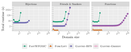
Figure 2: The runtime of the algorithms as a function of domain size. Note that both axes are on a logarithmic scale.

Figure˜2 presents a summary of the experimental results. Only FastWFOMC and Gantry-BFS could handle the bijection-counting problem. For this benchmark, the largest domain sizes these algorithms could accommodate were $64$ and $4096$, respectively. On the other two benchmarks, ForcLift had the lowest runtime. However, since it can only handle model counts smaller than $2^{31}$, it only scales up to domain sizes of $16$ and $128$ for Friends & Smokers and Functions, respectively. FastWFOMC outperformed ForcLift in the case of Friends & Smokers, but not Functions, as it could handle domains of size $1024$ and $64$, respectively. Furthermore, both Gantry-BFS and Gantry-Greedy performed similarly on both benchmarks. Similarly to the Bijections benchmark, Gantry significantly outperformed the other two algorithms, scaling up to domains of size $8192$ and $67,108,864$, respectively.

One might notice that the runtime of FastWFOMC and ForcLift is slightly higher for the smallest domain size. This peculiarity is the consequence of just-in-time (JIT) compilation. As Gantry is only run once per benchmark, we include the JIT compilation time in its overall runtime across all domain sizes. Additionally, while the compilation time of ForcLift is generally lower compared to Gantry, neither significantly affects the overall runtime. Specifically, ForcLift compilation typically takes around $0.5\text{\,}\mathrm{s}$, while Gantry compilation takes around $2.3\text{\,}\mathrm{s}$.

Based on our experiments, which algorithm should one use in practice? If ForcLift can handle the sentence and the domain sizes are reasonably small, it is likely the fastest algorithm. In other situations, Gantry will likely be significantly more efficient than FastWFOMC regardless of domain size, provided both algorithms can handle the sentence.

5 Conclusion and Future Work

In this work, we have presented a scalable, automated FOKC-based approach to FOMC. Our algorithm involves completing the definitions of recursive functions and subsequently translating all function definitions into C++ code. Empirical results demonstrate that Gantry can scale to larger domain sizes than FastWFOMC while supporting a wider range of sentences than ForcLift. The ability to efficiently handle large domain sizes is particularly crucial in the weighted setting, as illustrated by the Friends & Smokers example, where the model captures complex social networks with probabilistic relationships. Without this scalability, these models would have limited practical value.

Future directions for research include conducting a comprehensive experimental comparison of FOMC algorithms to better understand their comparative performance across various sentences. The capabilities of Gantry could also be characterised theoretically, for example, by proving completeness for logic fragments liftable by other algorithms [11, 22, 26]. Additionally, the efficiency of FOMC algorithms can be further analysed using fine-grained complexity, which would provide more detailed insights into the computational demands of different sentences.

Appendix A The Three Logics of FOMC

Logic	Sorts	Constants	Variables	Quantifiers	Additional atoms
$\mathsf{FO}$	one or more	✓	unlimited	$\forall$, $\exists$	$x=y$
$\mathsf{C}^{2}$	one	✗	two	$\forall$, $\exists$, $\exists^{=k}$, $\exists^{\leq k}$, $\exists^{\geq k}$	—
$\mathsf{UFO}^{2}+\mathsf{CC}$	one	✗	two	$\forall$	$|P|=m$

Table 1: A comparison of the three logics used in FOMC. The 2^nd–5^th columns refer to the number of sorts, support for constants, the maximum number of variables, and supported quantifiers, respectively. The last column lists supported atoms in addition to those of the form $P(\mathbf{t})$ for a predicate $P/n$ and an $n$-tuple of terms $\mathbf{t}$. Here, $k$ and $m$ are non-negative integers, where $m$ depends on the domain size, $P$ is a predicate, and $x$ and $y$ are terms.

FOMC commonly utilises three types of first-order logic: $\mathsf{FO}$, $\mathsf{C}^{2}$, and $\mathsf{UFO}^{2}+\mathsf{CC}$. Table˜1 summarises the key differences among them. $\mathsf{FO}$ is the input format for ForcLift and its extensions Crane and Gantry. $\mathsf{C}^{2}$ is often used in the literature on FastWFOMC and related methods [11, 12]. (Note that no algorithm accepts $\mathsf{C}^{2}$ as input.) Finally, $\mathsf{UFO}^{2}+\mathsf{CC}$ is the input format supported by the most recent implementation of FastWFOMC [23]. All three logics are function-free, and domains are always assumed to be finite. As usual, we presuppose the unique name assumption, which states that two constants are equal if and only if they are the same constant [18].

In $\mathsf{FO}$, each term has a designated sort, and each predicate $P/n$ corresponds to a sequence of $n$ sorts. Each sort has its corresponding domain. These assignments to sorts are typically left implicit and follow from the quantifiers, e.g., $\forall x,y\in\Delta\text{. }P(x,y)$ implies that the variables $x$ and $y$ have the same sort. On the other hand, $\forall x\in\Delta\text{. }\forall y\in\Gamma\text{. }P(x,y)$ implies that $x$ and $y$ have different sorts, and it would be improper to write, for example, $\forall x\in\Delta\text{. }\forall y\in\Gamma\text{. }P(x,y)\lor x=y$. $\mathsf{FO}$ is also the only logic to support constants, sentences with more than two variables, and the equality predicate. While we do not explicitly refer to sorts in the paper, the many-sorted nature of $\mathsf{FO}$ is paramount to the algorithms presented therein.

In the case of ForcLift and its extensions, support for a sentence as valid input does not imply that the algorithm can compile the sentence into a circuit or graph suitable for lifted model counting. However, ForcLift compilation always succeeds on any $\mathsf{FO}$ sentence without constants and with at most two variables [27, 29].

Compared to $\mathsf{FO}$, $\mathsf{C}^{2}$ and $\mathsf{UFO}^{2}+\mathsf{CC}$ lack support for constants, the equality predicate, multiple domains, and sentences with more than two variables. The advantage that $\mathsf{C}^{2}$ brings over $\mathsf{FO}$ is the inclusion of counting quantifiers. That is, alongside $\forall$ and $\exists$, $\mathsf{C}^{2}$ supports $\exists^{=k}$, $\exists^{\leq k}$, and $\exists^{\geq k}$ for any positive integer $k$. For example, $\exists^{=1}x\text{. }\phi(x)$ means that there exists exactly one $x$ such that $\phi(x)$, and $\exists^{\leq 2}x\text{. }\phi(x)$ means that there exist at most two such $x$. $\mathsf{UFO}^{2}+\mathsf{CC}$, on the other hand, does not support any existential quantifiers but instead incorporates (equality) cardinality constraints. For example, $|P|=3$ constrains all models to have precisely three positive literals with the predicate $P$.

Our Benchmarks in $\mathsf{C}^{2}$ and $\mathsf{UFO}^{2}+\mathsf{CC}$

For completeness and reproducibility, let us translate the benchmark sentences from $\mathsf{FO}$ to $\mathsf{C}^{2}$ and $\mathsf{UFO}^{2}+\mathsf{CC}$. Since Friends & Smokers is a relatively simple sentence, it remains the same in $\mathsf{C}^{2}$ and $\mathsf{UFO}^{2}+\mathsf{CC}$. For Functions, in $\mathsf{C}^{2}$, one would write

$$\forall x\in\Delta\text{. }\exists^{=1}y\in\Delta\text{. }P(x,y).$$

In $\mathsf{UFO}^{2}+\mathsf{CC}$, the equivalent formulation is

$$(\forall x,y\in\Delta\text{. }S(x)\lor\neg P(x,y))\land(|P|=|\Delta|),$$ (8)

where $w^{-}(S)=-1$. Although Equation˜8 has more models than its counterpart in $\mathsf{C}^{2}$, the negative weight $w^{-}(S)=-1$ causes some of the terms in the definition of WFOMC to cancel out. The translation of Bijections is similar to that of Functions. In $\mathsf{C}^{2}$, one could write

$$(\forall x\in\Delta\text{. }\exists^{=1}y\in\Delta\text{. }P(x,y))\land(\forall y\in\Delta\text{. }\exists^{=1}x\in\Delta\text{. }P(x,y)).$$

Similarly, in $\mathsf{UFO}^{2}+\mathsf{CC}$, the equivalent formulation is

$$(\forall x,y\in\Delta\text{. }R(x)\lor\neg P(x,y))\land(\forall x,y\in\Delta\text{. }S(x)\lor\neg P(y,x))\land(|P|=|\Delta|),$$

where $w^{-}(R)=w^{-}(S)=-1$.

References

- [1] Damiano Azzolini and Fabrizio Riguzzi. Lifted inference for statistical statements in probabilistic answer set programming. Int. J. Approx. Reason., 163:109040, 2023. doi:10.1016/J.IJAR.2023.109040.
- [2] Jáchym Barvínek, Timothy van Bremen, Yuyi Wang, Filip Zelezný, and Ondřej Kuželka. Automatic conjecturing of P-recursions using lifted inference. In ILP, volume 13191 of Lecture Notes in Computer Science, pages 17–25. Springer, 2021. doi:10.1007/978-3-030-97454-1_2.
- [3] Paul Beame, Guy Van den Broeck, Eric Gribkoff, and Dan Suciu. Symmetric weighted first-order model counting. In PODS, pages 313–328. ACM, 2015. doi:10.1145/2745754.2745760.
- [4] Mark Chavira and Adnan Darwiche. On probabilistic inference by weighted model counting. Artif. Intell., 172(6-7):772–799, 2008. doi:10.1016/J.ARTINT.2007.11.002.
- [5] Adnan Darwiche. On the tractable counting of theory models and its application to truth maintenance and belief revision. Journal of Applied Non-Classical Logics, 11(1-2):11–34, 2001. doi:10.3166/JANCL.11.11-34.
- [6] Paulius Dilkas and Vaishak Belle. Synthesising recursive functions for first-order model counting: Challenges, progress, and conjectures. In KR, pages 198–207, 2023. doi:10.24963/KR.2023/20.
- [7] Vibhav Gogate and Pedro M. Domingos. Probabilistic theorem proving. Commun. ACM, 59(7):107–115, 2016. doi:10.1145/2936726.
- [8] Eric Gribkoff, Dan Suciu, and Guy Van den Broeck. Lifted probabilistic inference: A guide for the database researcher. IEEE Data Eng. Bull., 37(3):6–17, 2014. URL: http://sites.computer.org/debull/A14sept/p6.pdf.
- [9] Manfred Jaeger and Guy Van den Broeck. Liftability of probabilistic inference: Upper and lower bounds. In StarAI@UAI, 2012. URL: https://starai.cs.kuleuven.be/2012/accepted/jaeger.pdf.
- [10] Kristian Kersting. Lifted probabilistic inference. In ECAI, volume 242 of Frontiers in Artificial Intelligence and Applications, pages 33–38. IOS Press, 2012. doi:10.3233/978-1-61499-098-7-33.
- [11] Ondřej Kuželka. Weighted first-order model counting in the two-variable fragment with counting quantifiers. J. Artif. Intell. Res., 70:1281–1307, 2021. doi:10.1613/JAIR.1.12320.
- [12] Sagar Malhotra and Luciano Serafini. Weighted model counting in FO2 with cardinality constraints and counting quantifiers: A closed form formula. In AAAI, pages 5817–5824. AAAI Press, 2022. doi:10.1609/AAAI.V36I5.20525.
- [13] Nils J. Nilsson. Probabilistic logic. Artif. Intell., 28(1):71–87, 1986. doi:10.1016/0004-3702(86)90031-7.
- [14] Feng Niu, Christopher Ré, AnHai Doan, and Jude W. Shavlik. Tuffy: Scaling up statistical inference in Markov logic networks using an RDBMS. Proc. VLDB Endow., 4(6):373–384, 2011. doi:10.14778/1978665.1978669.
- [15] Vilém Novák, Irina Perfilieva, and Jiri Mockor. Mathematical principles of fuzzy logic, volume 517. Springer Science & Business Media, 2012.
- [16] OEIS Foundation Inc. The On-Line Encyclopedia of Integer Sequences, 2025. Published electronically at http://oeis.org.
- [17] Fabrizio Riguzzi, Elena Bellodi, Riccardo Zese, Giuseppe Cota, and Evelina Lamma. A survey of lifted inference approaches for probabilistic logic programming under the distribution semantics. Int. J. Approx. Reason., 80:313–333, 2017. doi:10.1016/J.IJAR.2016.10.002.
- [18] Stuart Russell and Peter Norvig. Artificial Intelligence: A Modern Approach (4th Edition). Pearson, 2020.
- [19] Dragan Z. Šaletić. Graded logics. Interdisciplinary Description of Complex Systems: INDECS, 22(3):276–295, 2024.
- [20] Parag Singla and Pedro M. Domingos. Lifted first-order belief propagation. In AAAI, pages 1094–1099. AAAI Press, 2008. URL: http://www.aaai.org/Library/AAAI/2008/aaai08-173.php.
- [21] Martin Svatos, Peter Jung, Jan Tóth, Yuyi Wang, and Ondřej Kuželka. On discovering interesting combinatorial integer sequences. In IJCAI, pages 3338–3346. ijcai.org, 2023. doi:10.24963/IJCAI.2023/372.
- [22] Jan Tóth and Ondřej Kuželka. Lifted inference with linear order axiom. In AAAI, pages 12295–12304. AAAI Press, 2023. doi:10.1609/AAAI.V37I10.26449.
- [23] Jan Tóth and Ondřej Kuželka. Complexity of weighted first-order model counting in the two-variable fragment with counting quantifiers: A bound to beat. In KR, 2024. doi:10.24963/KR.2024/64.
- [24] Pietro Totis, Jesse Davis, Luc De Raedt, and Angelika Kimmig. Lifted reasoning for combinatorial counting. J. Artif. Intell. Res., 76:1–58, 2023. doi:10.1613/JAIR.1.14062.
- [25] Timothy van Bremen and Ondřej Kuželka. Faster lifting for two-variable logic using cell graphs. In UAI, volume 161 of Proceedings of Machine Learning Research, pages 1393–1402. AUAI Press, 2021. URL: https://proceedings.mlr.press/v161/bremen21a.html.
- [26] Timothy van Bremen and Ondřej Kuželka. Lifted inference with tree axioms. Artif. Intell., 324:103997, 2023. doi:10.1016/J.ARTINT.2023.103997.
- [27] Guy Van den Broeck. On the completeness of first-order knowledge compilation for lifted probabilistic inference. In NIPS, pages 1386–1394, 2011. URL: https://proceedings.neurips.cc/paper/2011/hash/846c260d715e5b854ffad5f70a516c88-Abstract.html.
- [28] Guy Van den Broeck, Arthur Choi, and Adnan Darwiche. Lifted relax, compensate and then recover: From approximate to exact lifted probabilistic inference. In UAI, pages 131–141. AUAI Press, 2012. URL: https://dslpitt.org/uai/displayArticleDetails.jsp?mmnu=1&smnu=2&article_id=2349&proceeding_id=28.
- [29] Guy Van den Broeck, Wannes Meert, and Adnan Darwiche. Skolemization for weighted first-order model counting. In KR. AAAI Press, 2014. URL: http://www.aaai.org/ocs/index.php/KR/KR14/paper/view/8012.
- [30] Guy Van den Broeck, Nima Taghipour, Wannes Meert, Jesse Davis, and Luc De Raedt. Lifted probabilistic inference by first-order knowledge compilation. In IJCAI, pages 2178–2185. IJCAI/AAAI, 2011. doi:10.5591/978-1-57735-516-8/IJCAI11-363.
- [31] Yuanhong Wang, Juhua Pu, Yuyi Wang, and Ondřej Kuželka. Lifted algorithms for symmetric weighted first-order model sampling. Artif. Intell., 331:104114, 2024. doi:10.1016/J.ARTINT.2024.104114.