Friedman-Ramanujan functions in random hyperbolic geometry and application to spectral gaps II

Abstract.

The core focus of this series of two articles is the study of the distribution of the length spectrum of closed hyperbolic surfaces of genus $g$, sampled randomly with respect to the Weil–Petersson probability measure. In the first article [2], we introduced a notion of local topological type ${\mathbf{T}}$, and established the existence of a density function $V_{g}^{\mathbf{T}}(\ell)$ describing the distribution of the lengths of all closed geodesics of type $\mathbf{T}$ in a genus $g$ hyperbolic surface. We proved that $V_{g}^{\mathbf{T}}(\ell)$ admits an asymptotic expansion in powers of $1/g$. We introduced a new class of functions, called Friedman–Ramanujan functions, and related it to the study of the spectral gap $\lambda_{1}$ of the Laplacian.

In this second part, we provide a variety of new tools allowing to compute and estimate the volume functions $V_{g}^{\mathbf{T}}(\ell)$. Notably, we construct new sets of coordinates on Teichmüller spaces, distinct from Fenchel–Nielsen coordinates, in which the Weil–Petersson volume has a simple form. These coordinates are tailored to the geodesics we study, and we can therefore prove nice formulae for their lengths. We use these new ideas, together with a notion of pseudo-convolutions, to prove that the coefficients of the expansion of $V_{g}^{\mathbf{T}}(\ell)$ in powers of $1/g$ are Friedman–Ramanujan functions, for any local topological type $\mathbf{T}$. We then exploit this result to prove that, for any $\epsilon>0$, $\lambda_{1}\geq\frac{1}{4}-\epsilon$ with probability going to one as $g\rightarrow+\infty$, or, in other words, typical hyperbolic surfaces have an asymptotically optimal spectral gap.

1. Introduction

1.1. Main results and motivations

For an integer $g\geq 2$, let $S_{g}$ be a fixed compact oriented surface of genus $g$ with no boundary. This is the second of a two-part article, studying the distribution of the length spectrum of a random hyperbolic metric $X$ on $S_{g}$. Our probability space is the moduli space $\mathcal{M}_{g}$ of hyperbolic structures on $S_{g}$, endowed with the Weil–Petersson measure $\mathbb{P}_{g}^{\mathrm{\scriptsize{WP}}}$ normalized to be a probability measure.

1.1.1. Local topological type and associated density

In the first part [2], we defined a notion of local topological type for a loop $\mathbf{c}$ [2, §4]. Intuitively, $\mathbf{T}$ corresponds to the topological datum of a loop $\mathbf{c}$ filling a surface $\mathbf{S}$, so that we know the topology of $\mathbf{c}$ and its regular neighbourhood, but not the way it is embedded in the ambient surface of genus $g$. Examples of local topological types include the type $\mathbf{s}$ “simple” (loops with no self-intersections), or the figure-eight (with exactly one self-intersection). We developed new tools allowing to study the following averages.

Definition 1.1.

Let ${\mathbf{T}}=[{\mathbf{S,c}}]_{\mathrm{loc}}$ be a local topological type. For any measurable function $F:\mathbb{R}_{\geq 0}\rightarrow\mathbb{C}$, bounded and compactly supported, we define the ${\mathbf{T}}$-average of $F$ to be

(1.1) $$\langle F\rangle_{g}^{{\mathbf{T}}}:=\mathbb{E}_{g}^{\mathrm{\scriptsize{WP}}}\Bigg{[}\sum_{\begin{subarray}{c}\gamma\in\mathcal{G}(X)\\ \gamma\in{\mathbf{T}}\end{subarray}}F(\ell_{X}(\gamma))\Bigg{]}$$

where $\mathbb{E}_{g}^{\mathrm{\scriptsize{WP}}}$ denotes the expectation on the moduli space $\mathcal{M}_{g}$ when the hyperbolic structure $X\in\mathcal{M}_{g}$ is chosen randomly according to the normalized Weil–Petersson measure $\mathbb{P}_{g}^{\mathrm{\scriptsize{WP}}}$, and

• $\mathcal{G}(X)$ is the set of primitive oriented closed geodesics for the metric $X$;

• for any $\gamma\in\mathcal{G}(X)$ , $\ell_{X}(\gamma)$ is the length of $\gamma$ for the hyperbolic metric $X$;

• $\gamma\in{\mathbf{T}}$ means that the sum is restricted to closed geodesics of local topological type ${\mathbf{T}}$.

Taking $F$ to be the indicator function ${\mathchoice{1\mskip-4.0mu{\rm{l}}}{1\mskip-4.0mu{\rm{l}}}{1\mskip-4.5mu{\rm{l}}}{1\mskip-5.0mu{\rm{l}}}}_{[a,b]}$ of an interval $[a,b]$, the average $\langle F\rangle_{g}^{{\mathbf{T}}}$ is the expected number of closed primitive geodesics of local topological type ${\mathbf{T}}$ and length in the interval $[a,b]$. In the case of the local topological type “simple”, denoted as $\mathbf{s}$, the condition $\gamma\in\mathbf{s}$ means that the sum is restricted to all simple primitive closed geodesics.

We proved in [2, Prop. 5.9] that the averages $\langle F\rangle_{g}^{{\mathbf{T}}}$ can be written in an integral form, against a density function $V_{g}^{\mathbf{T}}(\ell)$ which is, informally, the “proportion” of surfaces $X\in\mathcal{M}_{g}$ containing a primitive closed geodesic of length $\ell$ and local topological type $\mathbf{T}$. The formal definition is as follows.

Proposition 1.2.

For any local topological type ${\mathbf{T}}$, there exists a unique measurable function $V_{g}^{\mathbf{T}}:\mathbb{R}_{>0}\rightarrow\mathbb{R}_{\geq 0}$ such that, for any admissible test function $F$,

$$\langle F\rangle_{g}^{{\mathbf{T}}}=\frac{1}{V_{g}}\int_{0}^{+\infty}F(\ell)\,V_{g}^{{\mathbf{T}}}(\ell)\,\mathrm{d}\ell.$$

The functions $V_{g}^{{\mathbf{T}}}(\ell)$ are a fundamental object for the study of geodesics in random hyperbolic surface. However they have been little studied, except in the case of the local topological type “simple”. For simple closed geodesics, Mirzakhani showed in [8] that the functions $V_{g}^{\mathbf{T}}(\ell)$ are polynomial in $\ell$ (hence they are called volume polynomials), and that they can be computed explicitly for all genus $g$ by topological recursion. Otherwise, we call $\ell\mapsto V_{g}^{{\mathbf{T}}}(\ell)$ the volume function associated with local topological type ${\mathbf{T}}$ on surfaces of genus $g$.

The precise nature of the functions $V_{g}^{\mathbf{T}}$ is not known. One can deduce from [10, Theorem 8.1] that $V_{g}^{{\mathbf{T}}}(\ell)$ behaves like a power of $\ell$ to leading order as $\ell\rightarrow+\infty$ with $g$ fixed. We believe that, for local topological type other than “simple”, the function $\ell\mapsto V_{g}^{\mathbf{T}}(\ell)$ is not polynomial, but is exponentially close to one as $\ell\rightarrow+\infty$ with $g$ fixed.

1.1.2. Large-genus asymptotic expansion

The object of the paper is the large genus behaviour of the volume functions $V_{g}^{\mathbf{T}}$. We proved in the first article [2] that they admit expansions to any order in powers of $g^{-1}$, in the following sense.

Theorem 1.3 ([2, Thm. 1.5 and 5.14]).

For any local topological type ${\mathbf{T}}=[{\mathbf{S,c}}]_{\mathrm{loc}}$, there exists a unique family of measurable functions $(f_{k}^{{\mathbf{T}}})_{k\geq 0}$ such that, for any integer $K\geq 0$ and $g\geq 2$,

(1.2) $$\Big{|}\langle F\rangle_{g}^{{\mathbf{T}}}-\sum_{k=0}^{K}\frac{1}{g^{k}}\int_{0}^{+\infty}F(\ell)\,f_{k}^{{\mathbf{T}}}(\ell)\,\mathrm{d}\ell\Big{|}\leq\frac{C_{K,\mathbf{S}}}{g^{K+1}}\sup_{\ell\geq 0}\{(\ell+1)^{\alpha_{K}^{\mathbf{S}}}|F(\ell)|e^{\ell}\}$$

for any measurable function $F:\mathbb{R}_{\geq 0}\rightarrow\mathbb{R}$ bounded with compact support.

As the notation indicates, the exponents $\alpha_{K}^{\mathbf{S}}$ and the constant $C_{K,\mathbf{S}}$ depends on the filled surface ${\mathbf{S}}$ and the order $K$ of the expansion, but not on the loop ${\mathbf{c}}$ filling $\mathbf{S}$. In forthcoming applications of our results to the spectral gap of the Laplacian, this uniform behaviour with respect to all loops filling the same surface is important.

1.1.3. Statement of the main results

The main technical result of this paper may be summarised as follows, answering positively the question asked in the first part of this article [2].

Theorem 1.4.

Let ${\mathbf{T}}$ be a local topological type other than “simple”. For any $k\geq 0$, the function $\ell\mapsto f_{k}^{{\mathbf{T}}}(\ell)$ is a Friedman–Ramanujan function in the weak sense.

The notion of Friedman–Ramanujan function was introduced in [2]. A measurable function $f:\mathbb{R}_{\geq 0}\rightarrow\mathbb{R}$ is said to be a Friedman–Ramanujan function if there exists a polynomial function $p$ such that $f(\ell)-p(\ell)e^{\ell}$ grows at most like a polynomial multiple of $e^{\ell/2}$. Precise definitions follow in §1.2, together with a quantitative versions of our main result (Theorem 1.16).

Remark 1.5.

The case of the local topological type $\mathbf{s}$ is excluded because, in this case, the function $f_{k}^{\mathbf{s}}$ have pole of order one at $0$. We prove that $\ell\mapsto\ell f_{k}^{\mathbf{s}}(\ell)$ are Friedman–Ramanujan functions in [1] (see [2, Proposition 3.3] for more details).

Theorem 1.4 has already been obtained when $\mathbf{T}$ is a figure-eight, or more generally when the filled surface $\mathbf{S}$ has Euler characteristic $-1$, in the first part of this article [2]. For this relatively simple topological situation, we could use almost explicit expressions of the functions $(f_{k}^{{\mathbf{T}}})_{k\geq 0}$.

The present paper deals with general local topological types and uses entirely new methods, involving finding explicit expressions for the Weil–Petersson measure in coordinates other than the Fenchel–Nielsen ones, and for the lengths of non-simple geodesics in those coordinates.

This work is largely motivated by the question of estimating the gap at the bottom of the spectrum of the Laplacian, for typical hyperbolic surfaces, as detailed in [2, 4]. In the first part of this article [2], we used the result when ${\mathbf{S}}$ has Euler characteristic $-1$ to prove that typical surfaces have spectral gap at least $2/9-\epsilon$. More generally, our theorem (together with the variant presented in §12) implies the optimal lower bound $1/4-\epsilon$ on the spectral gap.

Theorem 1.6.

Denote by $\lambda_{1}(X)$ the first non-trivial eigenvalue of Laplacian on the hyperbolic surface $X$. Then, for any $\epsilon>0$,

(1.3) $$\mathbb{P}_{g}^{\mathrm{\scriptsize{WP}}}\left(\lambda_{1}(X)\geq\frac{1}{4}-\epsilon\right)\mathop{\longrightarrow}\limits_{g\rightarrow+\infty}1.$$

1.2. Full statement of the Friedman–Ramanujan property

Let us introduce a few definitions, and present our main result more precisely.

1.2.1. Definitions

We recall from [2] the strong and weak definitions of the class of Friedman–Ramanujan functions, directly inspired by J. Friedman’s seminal work on random graphs [6, Definition 2.1] where he proves the Alon conjecture.

Definition 1.7.

Let $\mathrm{N}\geq 1$. We define the class of functions $\mathcal{R}^{\mathrm{N}}$ as the set of locally integrable functions $f:\mathbb{R}_{\geq 0}\rightarrow\mathbb{C}$ such that there exists $c>0$ satisfying

(1.4) $$\forall\ell\geq 0,\quad|f(\ell)|\leq c(\ell+1)^{\mathrm{N}-1}e^{\frac{\ell}{2}}.$$

We let $\mathcal{R}=\bigcup_{\mathrm{N}\geq 1}\mathcal{R}^{\mathrm{N}}$. A locally integrable function $f:\mathbb{R}_{\geq 0}\rightarrow\mathbb{C}$ is said to be a Friedman–Ramanujan function if there exists a polynomial function $p$ such that

$$f(\ell)-p(\ell)e^{\ell}\in\mathcal{R}.$$

We denote as $\mathcal{F}$ the set of Friedman–Ramanujan function. For $f\in\mathcal{F}$, the function $\ell\mapsto p(\ell)e^{\ell}$ is uniquely defined, we call it the principal term of $f$.

Notation 1.8.

For an integer $\mathrm{K}\geq 0$, we denote as $\mathbb{C}_{\mathrm{K}-1}[\ell]$ the space of polynomials of degree strictly less than $\mathrm{K}$, and by $\mathbb{C}_{\mathrm{K}-1}[\ell]\,e^{\ell}$ the class of functions of the form $p(\ell)\,e^{\ell}$ where $p\in\mathbb{C}_{\mathrm{K}-1}[\ell]$. Note that these sets are reduced to the constant function equal to $0$ if $\mathrm{K}=0$.

Definition 1.9.

For $\mathrm{K}\geq 0$, we denote as $\mathcal{F}^{\mathrm{K}}$ the subset of Friedman–Ramanujan functions of principal term in $\mathbb{C}_{\mathrm{K}-1}[\ell]\,e^{\ell}$, and for $\mathrm{N}\geq 1$, $\mathcal{F}^{\mathrm{K},\mathrm{N}}:=\mathbb{C}_{\mathrm{K}-1}[\ell]\,e^{\ell}\oplus\mathcal{R}^{\mathrm{N}}$.

Note that the space $\mathcal{R}$ can be identified with the subset $\mathcal{F}^{0}$ of Friedman–Ramanujan functions with principal term $p=0$, and similarily $\mathcal{R}^{\mathrm{N}}=\mathcal{F}^{0,\mathrm{N}}$.

In our proof of Theorem 1.4 we will rather use the following weak version of the classes $\mathcal{R}$ and $\mathcal{F}$. Remark that in the work of Friedman, where the functions are defined on $\mathbb{Z}_{>0}$ instead of $\mathbb{R}_{\geq 0}$, this distinction between weak and strong definition does not exist.

Definition 1.10.

Let $\mathrm{N}\geq 1$. We define the class of functions $\mathcal{R}_{w}^{\mathrm{N}}$ as the set of locally integrable functions $f:\mathbb{R}_{\geq 0}\rightarrow\mathbb{C}$ such that there exists $c>0$ satisfying

(1.5) $$\forall\ell\geq 0,\quad\int_{0}^{\ell}|f(s)|\,\mathrm{d}s\leq c(\ell+1)^{\mathrm{N}-1}e^{\frac{\ell}{2}}.$$

We let $\mathcal{R}_{w}=\bigcup_{\mathrm{N}\geq 1}\mathcal{R}_{w}^{\mathrm{N}}$. A locally integrable function $f:\mathbb{R}_{\geq 0}\rightarrow\mathbb{C}$ is said to be a Friedman–Ramanujan function in the weak sense if there exists a polynomial function $p$ such that

$$f(\ell)-p(\ell)e^{\ell}\in\mathcal{R}_{w}.$$

For $\mathrm{K}\geq 0$, we write $\mathcal{F}_{w}^{\mathrm{K}}:=\mathbb{C}_{\mathrm{K}-1}[\ell]\,e^{\ell}\oplus\mathcal{R}_{w}$ and for $\mathrm{N}\geq 1$, $\mathcal{F}^{\mathrm{K},\mathrm{N}}_{w}:=\mathbb{C}_{\mathrm{K}-1}[\ell]\,e^{\ell}\oplus\mathcal{R}^{\mathrm{N}}_{w}$.

As the name suggests, the strong definition implies the weak one.

Remark 1.11.

The property $f\in\mathcal{R}_{w}$ is equivalent to the definition given in [2], that is, the existence of $a>0$ such that

(1.6) $$\int_{0}^{+\infty}\frac{|f(\ell)|}{(\ell+1)^{a}e^{\frac{\ell}{2}}}\,\mathrm{d}\ell<+\infty.$$

More precisely, if $f\in\mathcal{R}^{\mathrm{N}}_{w}$, then (1.6) holds for any exponent $a>\mathrm{N}$. Conversely if (1.6) holds, then $f\in\mathcal{R}^{a+1}_{w}$.

1.2.2. Norms on the set of Friedman–Ramanujan functions

Let us define a norm on the spaces $\mathcal{F}^{\mathrm{K},\mathrm{N}}$ and $\mathcal{F}^{\mathrm{K},\mathrm{N}}_{w}$, which captures the size of the principal term and the remainder of the Friedman–Ramanujan function.

Notation 1.12.

For a polynomial function $p\in\mathbb{C}[\ell]$, we define $\|p\|_{\ell^{\infty}}$ to be the maximum modulus of the coefficients of $p$.

Definition 1.13.

For $\mathrm{N}\geq 1$, we define a norm on $\mathcal{R}^{\mathrm{N}}$ and $\mathcal{R}_{w}^{\mathrm{N}}$ by

$$\lVert f\rVert_{\mathcal{R}^{\mathrm{N}}}:=\sup_{\ell\geq 0}\frac{|f(\ell)|}{(\ell+1)^{\mathrm{N}-1}e^{\frac{\ell}{2}}}\quad\text{and}\quad\lVert f\rVert^{w}_{\mathcal{R}^{\mathrm{N}}}:=\sup_{\ell\geq 0}\frac{\int_{0}^{\ell}|f(s)|\,\mathrm{d}s}{(\ell+1)^{\mathrm{N}-1}\,e^{\frac{\ell}{2}}}.$$

If now $\mathrm{K}\geq 0$, we equip $\mathcal{F}^{\mathrm{K},\mathrm{N}}$ with the norm

$$\|f\|_{\mathcal{F}^{\mathrm{K},\mathrm{N}}}:=\|p\|_{\ell^{\infty}}+\|f(\ell)-p(\ell)e^{\ell}\|_{\mathcal{R}^{\mathrm{N}}}$$

where $p(\ell)\,e^{\ell}$ is the principal term of $f$. The norm $\|f\|_{\mathcal{F}^{\mathrm{K},\mathrm{N}}}^{w}$ is defined the same way replacing the last norm by its weak version.

It will be convenient to adopt the following convention.

Notation 1.14.

We denote as $\mathrm{fn}((u_{i})_{i\in\mathcal{V}})$ any quantity that is a function solely of some set of variables $(u_{i})_{i\in\mathcal{V}}$ (but for which we do not need to write an explicit expression).

Remark 1.15.

By definition, if $f\in\mathcal{R}^{\mathrm{N}}$, then for all $\ell\geq 0$,

(1.7) $$|f(\ell)|\leq\lVert f\rVert_{\mathcal{R}^{\mathrm{N}}}\,(1+\ell)^{\mathrm{N}-1}e^{\ell/2}.$$

If we rather assume that $f\in\mathcal{F}^{\mathrm{K},\mathrm{N}}$, then for $\ell\geq 0$,

(1.8) $$|f(\ell)|\leq\mathrm{fn}(\mathrm{K},\mathrm{N})\lVert f\rVert_{\mathcal{F}^{\mathrm{K},\mathrm{N}}}\,(1+\ell)^{\mathrm{K}-1}e^{\ell}$$

for some constant $\mathrm{fn}(\mathrm{K},\mathrm{N}):=1+\sup_{\ell\geq 0}(1+\ell)^{\mathrm{N}-\mathrm{K}}e^{-\ell/2}$.

1.2.3. Precise statement

The main technical result of this paper is the following precised version of Theorem 1.4.

Theorem 1.16.

Let ${\mathbf{T}}=[{\mathbf{S,c}}]_{\mathrm{loc}}$ be a local type other than “simple”. Then, for any $k\geq 0$, there exist $\mathrm{K},\mathrm{N}$ and $C$, depending on $k$ and ${\mathbf{S}}$ but not on ${\mathbf{c}}$, such that $f_{k}^{{\mathbf{T}}}\in\mathcal{F}_{w}^{\mathrm{K},\mathrm{N}}$ and $\lVert f_{k}^{{\mathbf{T}}}\rVert_{\mathcal{F}^{\mathrm{K},\mathrm{N}}}^{w}\leq C$.

Notation 1.17.

We denote as $(g_{\mathbf{S}},n_{\mathbf{S}})$ the signature of $\mathbf{S}$, and $\chi(\mathbf{S}):=2g_{\mathbf{S}}-2+n_{\mathbf{S}}$ its absolute Euler characteristic. We denote as $\partial\mathbf{S}$ the set of boundary components of $\mathbf{S}$, which is identified with $\{1,\ldots,n_{\mathbf{S}}\}$ through the labelling of the boundary of $\mathbf{S}$.

Remark 1.18.

The proof gives a seemingly optimal estimate on $\mathrm{K}$, and a non-optimal estimate on $\mathrm{N}$ and $C$: we may take $\mathrm{K}=2k+2\chi(\mathbf{S})$ and $\mathrm{N}=n_{\mathbf{S}}(a_{k+1}+1)$, where $a_{k+1}$ is an explicit sequence coming from [1] which is a priori not optimal either. Remark 1.25 show how we may optimise further the value of $\mathrm{K}$, depending on the topology of the multi-loop $\mathbf{c}$.

1.3. Outline of the proof

Let ${\mathbf{T}}=[{\mathbf{S,c}}]_{\mathrm{loc}}$ be a local topological type, i.e. the topological datum of a loop $\mathbf{c}$ filling a surface $\mathbf{S}$. We present prior results on the volume function $V_{g}^{\mathbf{T}}$ and the coefficients $(f_{k}^{\mathbf{T}})_{k\geq 0}$ of its asymptotic expansion in powers of $1/g$. We then explain the key ideas behind the proof of the main theorem.

1.3.1. Teichmüller spaces and the Weil–Petersson measure

For $\mathbf{x}=(x_{1},\ldots,x_{n_{\mathbf{S}}})\in\mathbb{R}_{>0}^{n_{\mathbf{S}}}$, we denote as $\mathcal{T}_{g_{\mathbf{S}},n_{\mathbf{S}}}(\mathbf{x})$ the Teichmüller space of hyperbolic surfaces of genus $g_{\mathbf{S}}$ with $n_{\mathbf{S}}$ labelled geodesic boundary components of respective lengths $x_{1},\ldots,x_{n_{\mathbf{S}}}$. This space is a real-analytic manifold of dimension $6g_{\mathbf{S}}-6+2n_{\mathbf{S}}$. It is equipped with the Weil–Petersson symplectic form, which induces a volume that we call the Weil–Petersson measure and denote as $\mathrm{Vol}^{\mathrm{WP}}_{g_{\mathbf{S}},n_{\mathbf{S}},\mathbf{x}}$.

In this article, it will be more interesting to view the boundary lengths as free variables, and hence introduce the Teichmüller space

$$\mathcal{T}_{g_{\mathbf{S}},n_{\mathbf{S}}}^{*}=\{(\mathbf{x},Y)\,:\mathbf{x}\in\mathbb{R}_{>0}^{n_{\mathbf{S}}},Y\in\mathcal{T}_{g_{\mathbf{S}},n_{\mathbf{S}}}(\mathbf{x})\},$$

which is the space of compact hyperbolic metrics on the surface $\mathbf{S}$. The space $\mathcal{T}_{g_{\mathbf{S}},n_{\mathbf{S}}}^{*}$ is a real-analytic manifold of dimension $6g_{\mathbf{S}}-6+3n_{\mathbf{S}}=3\chi(\mathbf{S})$. It may be endowed with the positive measure $\,\mathrm{d}\mathrm{Vol}^{\mathrm{WP}}_{g_{\mathbf{S}},n_{\mathbf{S}}}(\mathbf{x},Y):=\,\mathrm{d}\mathbf{x}\,\mathrm{d}\mathrm{Vol}^{\mathrm{WP}}_{g_{\mathbf{S}},n_{\mathbf{S}}}(Y)$, where $\,\mathrm{d}\mathbf{x}$ is the Lebesgue measure on $\mathbb{R}_{>0}^{n_{\mathbf{S}}}$, which we also call Weil–Petersson measure. We will sometimes omit the mention of $\mathbf{x}$ and simply write $Y\in\mathcal{T}_{g_{\mathbf{S}},n_{\mathbf{S}}}^{*}$ when it is not useful to emphasize the boundary length of $Y$.

1.3.2. Level-set desintegration

The map $\mathcal{T}_{g_{\mathbf{S}},n_{\mathbf{S}}}^{*}\ni Y\mapsto\ell_{Y}({\mathbf{c}})$ is a non-constant analytic function on the Teichmüller space $\mathcal{T}_{g_{\mathbf{S}},n_{\mathbf{S}}}^{*}$. We can therefore desintegrate the Weil–Petersson measure $\,\mathrm{d}\mathrm{Vol}^{\mathrm{WP}}_{g_{\mathbf{S}},n_{\mathbf{S}}}$ on its level-sets. This yields a measure $\,\mathrm{d}\mathrm{Vol}^{\mathrm{WP}}_{g_{\mathbf{S}},n_{\mathbf{S}}}(Y)/\,\mathrm{d}\ell$ defined by the property that, for any integrable function $F:\mathcal{T}_{g_{\mathbf{S}},n_{\mathbf{S}}}^{*}\rightarrow\mathbb{R}_{\geq 0}$, we have

$$\int_{\mathcal{T}_{g_{\mathbf{S}},n_{\mathbf{S}}}^{*}}F(Y)\,\mathrm{d}\mathrm{Vol}^{\mathrm{WP}}_{g_{\mathbf{S}},n_{\mathbf{S}}}(Y)=\int_{0}^{+\infty}\Big{(}\int_{\begin{subarray}{c}\ell_{Y}({\mathbf{c}})=\ell\end{subarray}}F(Y)\frac{\,\mathrm{d}\mathrm{Vol}^{\mathrm{WP}}_{g_{\mathbf{S}},n_{\mathbf{S}}}(Y)}{\,\mathrm{d}\ell}\Big{)}\,\mathrm{d}\ell.$$

In particular, if $F(\mathbf{x},Y)=\tilde{F}(\ell_{Y}({\mathbf{c}}))\phi(\mathbf{x})$ is a multiplicative function of $\ell_{Y}({\mathbf{c}})$ and $\mathbf{x}$, this equation takes the special form

$$\int_{\mathcal{T}_{g_{\mathbf{S}},n_{\mathbf{S}}}^{*}}\tilde{F}(\ell_{Y}({\mathbf{c}}))\phi(\mathbf{x})\,\mathrm{d}\mathrm{Vol}^{\mathrm{WP}}_{g_{\mathbf{S}},n_{\mathbf{S}}}(\mathbf{x},Y)=\int_{0}^{+\infty}\tilde{F}(\ell)\Big{(}\int_{\ell_{Y}({\mathbf{c}})=\ell}\phi(\mathbf{x})\frac{\,\mathrm{d}\mathrm{Vol}^{\mathrm{WP}}_{g,n}(\mathbf{x},Y)}{\,\mathrm{d}\ell}\Big{)}\,\mathrm{d}\ell.$$

1.3.3. Description of the volume function and coefficients

We have proven in [2] that the volume function $V_{g}^{{\mathbf{T}}}(\ell)$ and the coefficients $f_{k}^{{\mathbf{T}}}(\ell)$ are all of the form

(1.9) $$\ell\mapsto\int_{\ell_{Y}({\mathbf{c}})=\ell}\phi(\mathbf{x})\frac{\,\mathrm{d}\mathrm{Vol}^{\mathrm{WP}}_{g_{\mathbf{S}},n_{\mathbf{S}}}(\mathbf{x},Y)}{\,\mathrm{d}\ell},$$

with particular choices of $\phi(\mathbf{x})$.

More precisely, the volume function $V_{g}^{{\mathbf{T}}}(\ell)$ is obtained by replacing $\phi$ with the following explicit polynomial function:

(1.10) $$\Phi_{g}^{\mathbf{T}}(\mathbf{x}):=\frac{1}{m(\mathbf{T})}\frac{x_{1}\ldots x_{n_{\mathbf{S}}}}{V_{g}}\sum_{\mathfrak{R}\in R_{g}({\mathbf{S}})}V_{\mathfrak{R}}(\mathbf{x}),$$

which enumerates all possible embeddings of $\mathbf{S}$ in a surface of genus $g$ (the coefficient $m(\mathbf{T})$ is a combinatorial factor, and $V_{\mathfrak{R}}(\mathbf{x})$ are products of volumes of moduli spaces, enumerated by configurations ${\mathfrak{R}}\in R_{g}(\mathbf{S})$).

From this expression, the functions $f_{k}^{{\mathbf{T}}}(\ell)$ are then obtained by performing the asymptotic expansion of $\Phi_{g}^{\mathbf{T}}(\mathbf{x})$ in powers of $1/g$, using the results of [1, 2]. It follows that $f_{k}^{{\mathbf{T}}}(\ell)$ has the form (1.9) for a $\phi(\mathbf{x})$ which is a linear combination of functions

(1.11) $$\prod_{i\in V_{0}}x_{i}^{k_{i}}\prod_{i\in V_{+}}x_{i}^{k_{i}}\cosh\left(\frac{x_{i}}{2}\right)\prod_{i\in V_{-}}x_{i}^{k_{i}}\sinh\left(\frac{x_{i}}{2}\right)\prod_{j=1}^{k}x_{i_{j}}\delta(x_{i_{j}}-x_{i_{j}^{\prime}}),$$

where:

• $V_{0}$, $V_{+}$, $V_{-}$ are three disjoint subsets of $\partial\mathbf{S}$;

• $\mathrm{m}=\bigsqcup_{j=1}^{k}\{i_{j},i_{j}^{\prime}\}$ is a perfect matching of $\partial\mathbf{S}\setminus(V_{0}\sqcup V_{+}\sqcup V_{-})$;

• $\delta$ is the usual Dirac mass.

The degree $k_{i}$ is odd if $i\in V_{0}\cup V_{+}$ and even if $i\in V_{-}$. In [1] we proved that $\sum_{i\in V_{+}\cup V_{-}}k_{i}\leq 2k$, and that for $i\in V_{0}$, we have $k_{i}\leq a_{k+1}$ for a certain sequence $a_{k+1}$ (which is explicit but a priori not optimal).

1.3.4. Brief reminder about the method followed in [1, 2]

It is worth now recalling the main steps in the proof of the asymptotic expansion of $\Phi_{g}^{\mathbf{T}}(\mathbf{x})$.

Notation 1.19.

Throughout this article, we shall use the Landau notation $\mathcal{O}$, i.e. we will write $A=\mathcal{O}\left(B\right)$ if there exists a constant $c>0$ such that, for any choice of parameters, $|A|\leq cB$. If the constant $c$ depends on some parameters, we shall write them as a subscript of the $\mathcal{O}$.

• First, we note that, although the cardinality of $R_{g}({\mathbf{S}})$ in (1.10) grows with $g$, we can identify a set of embeddings $R_{g}({\mathbf{S}},K)$ of bounded cardinality, such that

  $$\Phi_{g}^{\mathbf{T}}(\mathbf{x})=\frac{1}{m(\mathbf{T})}\frac{x_{1}\ldots x_{n_{\mathbf{S}}}}{V_{g}}\sum_{{\mathfrak{R}}\in R_{g}({\mathbf{S}},K)}V_{\mathfrak{R}}(\mathbf{x})+\mathcal{O}_{K,n_{\mathbf{S}}}\left(\frac{(\lVert\mathbf{x}\rVert+1)^{\alpha_{K}^{\mathbf{S}}}e^{\frac{x_{1}+\ldots+x_{n_{\mathbf{S}}}}{2}}}{g^{K+1}}\right).$$

  This is done in [2, Proposition 5.21] and its proof.

• Then, for each realisation ${\mathfrak{R}}\in R_{g}({\mathbf{S}},K)$, we observe that there exist integers $n_{1}\leq n_{\mathbf{S}}$ and $m\leq(K+n_{\mathbf{S}})/2$ such that the ratio $V_{\mathfrak{R}}(\mathbf{x})/V_{\mathfrak{R}}(0)$ coincides (modulo permutation of the variables) with $V_{g-m,n_{1}}(x_{1},\ldots,x_{n_{1}})/V_{g-m,n_{1}}$ multiplied by a fixed polynomial in $(x_{n_{1}+1},\ldots,x_{n_{\mathbf{S}}})$. We recall that, for any $g,n$ with $2g-2+n>0$, $V_{g,n}$ denotes the constant coefficient of the volume polynomial $V_{g,n}(\cdot)$, i.e. its value at $(0,\ldots,0)$.

• The main result of [1] says that $V_{g-m,n_{1}}(x_{1},\ldots,x_{n_{1}})/V_{g-m,n_{1}}$ coincides, modulo a remainder in $\mathcal{O}_{K,n_{1}}\left((\lVert\mathbf{x}\rVert+1)^{\alpha_{K}^{n_{1}}}e^{\frac{x_{1}+\ldots+x_{n_{1}}}{2}}/g^{K+1}\right)$, with a linear combination of the functions (1.11), with degree $k_{i}\leq a_{K+1}$, the coefficients being of the form

  $$A_{V_{0},V_{+},V_{-}}(n_{1},m,K,k_{1},\ldots,k_{n_{1}})\,\,\frac{c_{g-m,n_{1}}(\alpha)}{V_{g-m,n_{1}}}$$

  and $\|\alpha\|_{\infty}\leq 2K+a_{K+1}$. Here $a_{K+1}$ is a sequence introduced in [2], and $c_{g-m,n_{1}}(\alpha)$ is our notation for the coefficients of volume polynomials.

• At the end we inject the result of Mirzakhani–Zograf [11, Theorem 4.1], showing the existence of an asymptotic expansion in powers of $g^{-1}$ for $c_{g-m,n_{1}}(\alpha)/V_{g-m,n_{1}}$ and for $V_{\mathfrak{R}}(0)/V_{g}$, and hence for $c_{g-m,n_{1}}(\alpha)/V_{g}$.

Remark 1.20.

The last step is only necessary if we insist on obtaining an expansion $V_{g}^{{\mathbf{T}}}(\ell)$ in powers of $g^{-1}$. The three first steps, together with the fact that $\frac{c_{g-m,n_{1}}(\alpha)}{V_{g-m,n_{1}}}$ and $\frac{V_{\mathfrak{R}}(0)}{V_{g}}$ are bounded functions of $g$, are actually sufficient to obtain the spectral gap (Theorem 1.6).

Until §12, the surface $\mathbf{S}$ is fixed and we do not need to know how $A_{V_{0},V_{+},V_{-}}(n_{1},m,K,k_{1},\ldots,k_{n_{1}})$ depend on $n_{1}$. In §12, we will need to come back to the proof of the asymptotic expansion, in order to have a very rough control of the dependency on $n_{1},n_{\mathbf{S}}$ of those coefficients, as well as the constants involved in $\mathcal{O}_{K,n_{\mathbf{S}}}{}$ and $\mathcal{O}_{K,n_{1}}{}$.

1.3.5. Unshielded simple portions

The following topological quantity, associated to a local topological type, will appear in our abstract statement.

Definition 1.21.

Let $\mathbf{T}=[\mathbf{S},\mathbf{c}]_{\mathrm{loc}}$ be a local topological type.

1. A simple portion of $\mathbf{c}$ is a maximal open subsegment of $\mathbf{c}$ which does not contain any self-intersection point of $\mathbf{c}$.

2. A simple portion is said to be shielded if it belongs to the boundary of a contractible component of $\mathbf{S}\setminus\mathbf{c}$, and unshielded otherwise.

3. We say $\mathbf{c}$ is double-filling if all simple portions are shielded.

We denote by $\rho[{\mathbf{T}}]$ the number of unshielded simple portions of $\mathbf{T}$.

The notion of simple portion and double-filling multi-loop appeared in our previous paper [2, Notation 8.3]. We have the inequality $\rho[{\mathbf{T}}]\leq 2\chi(\mathbf{S})$, which means that the number of unshielded simple portions is bounded uniformly in $\mathbf{c}$.

1.3.6. Main abstract statement

We can use (1.11) to reduce the proof of Theorem 1.16 to a general abstract statement, which we shall now state and comment. Because our main theorem requires quite a few notation, we group them below.

Notation 1.22 (Assumptions for main theorem).

• Let $\mathbf{T}=[\mathbf{S},\mathbf{c}]_{\mathrm{loc}}$ be a local type of signature $(g_{\mathbf{S}},n_{\mathbf{S}})$. We denote as $\rho[{\mathbf{T}}]$ be the number of unshielded simple portions of ${\mathbf{T}}$.

• Let $V$ be a subset of $\partial\mathbf{S}$ such that $n_{\mathbf{S}}-\#V=2k$ is even, and $\mathrm{m}$ be a perfect matching of $\partial\mathbf{S}\setminus V$, that is, a partition $\{1,\ldots,n_{\mathbf{S}}\}\setminus V=\bigsqcup_{j=1}^{k}\{i_{j},i_{j}^{\prime}\}$.

• We fix a smooth function $\chi_{\textrm{z}}$ that vanishes at order $1$ at $x=0$ and is constant equal to $1$ on $[1,+\infty)$, and such that

  (1.12) $$\Big{|}\frac{\chi_{\textrm{z}}(y)^{2}}{(1-e^{-y})^{2}}-1\Big{|}\leq 8e^{-y}.$$

• For $j\in V$, let $f_{j}$ be a function such that $\tilde{g}_{j}(x):=f_{j}(x)\sinh\left(\frac{x}{2}\right)/\chi_{\textrm{z}}(x)^{2}$ is continuous and lies in $\mathcal{F}^{\mathrm{K}_{j},\mathrm{N}_{j}}$ for some integers $\mathrm{K}_{j}$ and $\mathrm{N}_{j}$. We assume w.l.o.g. that $\mathrm{K}_{j}\leq\mathrm{N}_{j}$. We set

  $$\mathrm{K}=\sum_{j\in V}(\mathrm{K}_{j}-1)+\rho[\mathbf{T}]\qquad\text{and}\qquad\mathrm{N}=\sum_{j\in V}\mathrm{N}_{j}+3\chi(\mathbf{S})+1.$$

Theorem 1.23.

With the assumptions from Notation 1.22, the function

(1.13) $$\mathcal{J}=\mathcal{J}_{\mathbf{T},V,\mathrm{m},f}:\ell\mapsto\int_{\begin{subarray}{c}(\mathbf{x},Y)\in\mathcal{T}^{*}_{g_{\mathbf{S}},n_{\mathbf{S}}}\\ \ell_{Y}({\mathbf{c}})=\ell\end{subarray}}\,\,\prod_{j\in V}f_{j}(x_{j})\prod_{j=1}^{k}x_{i_{j}}\delta(x_{i_{j}}-x_{i_{j}^{\prime}})\frac{\,\mathrm{d}\mathrm{Vol}^{\mathrm{WP}}_{g_{\mathbf{S}},n_{\mathbf{S}}}(\mathbf{x},Y)}{\,\mathrm{d}\ell}$$

is a Friedman–Ramanujan function in the weak sense. More precisely, $\mathcal{J}\in\mathcal{F}_{w}^{\mathrm{K},\mathrm{N}}$ and

(1.14) $$\lVert\mathcal{J}\rVert^{w}_{\mathcal{F}^{\mathrm{K},\mathrm{N}}}\leq\mathrm{fn}(g_{\mathbf{S}},n_{\mathbf{S}},(\mathrm{K}_{j},\mathrm{N}_{j})_{j\in V})\,\prod_{j\in V}\lVert\tilde{g}_{j}\rVert_{\mathcal{F}^{\mathrm{K}_{j},\mathrm{N}_{j}}}.$$

Remark 1.24.

Since $\rho[{\mathbf{T}}]\leq 2\chi(\mathbf{S})$, our Friedman–Ramanujan exponents $\mathrm{K}$ and $\mathrm{N}$ can be made uniform amongst all loops filling $\mathbf{S}$.

Remark 1.25.

In the proof of Theorem 1.23, we have tried to optimise the value of $\mathrm{K}$, but not the value of $\mathrm{N}$. One can further improve the value of $\mathrm{K}$ depending on the loop $\mathbf{c}$, and prove that it can be taken to be $\sum_{j\in V^{\prime}}(\mathrm{K}_{j}-1)+\rho[\mathbf{T}]$, where $V^{\prime}\subseteq V$ is the set of boundary components containing unshielded simple portions of $\mathbf{c}$. See details in Remark 11.24.

We notice that in the special case when the loop $\mathbf{c}$ is double-filling, we have $V^{\prime}=\emptyset$ and $\rho[\mathbf{T}]=0$. In other words, the function $\mathcal{J}$ is actually an element of $\mathcal{R}_{w}$ as soon as $\mathbf{c}$ is double-filling.

Let us now show how to go from Theorem 1.23 to Theorem 1.16.

Proof of Theorem 1.16.

We simply use the expression (1.11) for the functions $f_{k}^{\mathbf{T}}$, and apply our main technical result to $V=V_{0}\sqcup V_{+}\sqcup V_{-}$ and the functions

$$f_{j}(x)=\begin{cases}x_{j}^{k_{j}}&\text{if }j\in V_{0}\\ x_{j}^{k_{j}}\cosh\left(\frac{x_{j}}{2}\right)&\text{if }j\in V_{+}\\ x_{j}^{k_{j}}\sinh\left(\frac{x_{j}}{2}\right)&\text{if }j\in V_{-}\end{cases}$$

which clearly satisfy the hypotheses with

$$\begin{cases}\mathrm{K}_{j}=\mathrm{N}_{j}=k_{j}+1&\text{if }j\in V_{+}\cup V_{-}\\ \mathrm{K}_{j}=0,\mathrm{N}_{j}=a_{k+1}+1&\text{if }j\in V_{0},\end{cases}$$

using the parity condition on the integers $k_{j}$ to obtain the needed cancellation at $0$. ∎

Remark 1.26.

The proof above allows us to see that, in Theorem 1.16, we may take the Friedman–Ramanujan parameters to be

$$\mathrm{K} =\sum_{j\in V_{+}\cup V_{-}}k_{j}+\rho[{\mathbf{T}}]\leq 2k+\rho[{\mathbf{T}}]\leq 2k+2\chi(\mathbf{S})$$

$$\mathrm{N} =\sum_{j\in V_{0}\cup V_{+}\cup V_{-}}\mathrm{N}_{j}+3\chi(\mathbf{S})+1\leq n_{\mathbf{S}}(a_{k+1}+1)+3\chi(\mathbf{S})+1.$$

The proof of Theorem 1.6 about the spectral gap of random surfaces requires variants of Theorem 1.23. A first straightforward variant is that Theorem 1.23 also applies in the case where $\mathbf{c}$ is a multi-loop, defined as a collection of loops (§2.1.1). Another variant will be given in Theorem 9.4 (where some of the loops in $\mathbf{c}$ are constrained to have bounded lengths). The final variant needed for the spectral gap is described in §12.

1.3.7. Friedman–Ramanujan functions as solutions of an integral equation

A first ingredient in the proof of Theorem 1.23 is the fact that Friedman–Ramanujan functions are fully characterised as solutions (modulo $\mathcal{R}$) of a certain integral equation. We define two operators acting on locally integrable functions, $\mathcal{P}=\mathcal{P}_{x}=\int_{0}^{x}$ (taking the primitive vanishing at $0$) and $\mathcal{L}=\mathcal{L}_{x}=\operatorname{id}-\mathcal{P}_{x}$ (where $\operatorname{id}$ stands for the identity operator). It is trivial, nevertheless useful, to note that $\mathcal{P}$ and $\mathcal{L}$ preserve $\mathcal{F},\mathcal{F}_{w},\mathcal{R},\mathcal{R}_{w}$. More precisely, $\mathcal{L}$ is a continuous operator from $\mathcal{F}^{\mathrm{K}}$ to $\mathcal{F}^{\mathrm{K}-1}$ and from $\mathcal{R}$ to itself (and this is also true for the weak spaces).

We will make use of the following characterization of Friedman–Ramanujan functions:

Proposition 1.27.

For $\mathrm{K}\geq 1$, any locally integrable function $f$,

$$\begin{cases}f\in\mathcal{F}^{\mathrm{K}}\Leftrightarrow\mathcal{L}^{\mathrm{K}}f\in\mathcal{R}\\ f\in\mathcal{F}^{\mathrm{K}}_{w}\Leftrightarrow\mathcal{L}^{\mathrm{K}}f\in\mathcal{R}_{w}.\end{cases}$$

Furthermore, if $\mathrm{N}\geq 1$ is so that $\mathcal{L}^{\mathrm{K}}f\in\mathcal{R}^{\mathrm{N}}_{w}$, then

(1.15) $$\lVert f\rVert_{\mathcal{F}^{\mathrm{K},\mathrm{N}}}^{w}\leq\mathrm{fn}(\mathrm{K},\mathrm{N})\,\lVert\mathcal{L}^{\mathrm{K}}f\rVert^{w}_{\mathcal{R}^{\mathrm{N}}}.$$

The “only if” part is a straightforward consequence of the fact that $\mathcal{L}$ sends $\mathcal{R}_{w}$ to itself, $\mathcal{R}$ to itself, and that $\mathcal{L}^{\mathrm{K}}$ sends $\mathbb{C}_{\mathrm{K}-1}[t]e^{t}$ to $\mathbb{C}_{\mathrm{K}-1}[t]\subset\mathcal{R}$. The “if” part is proven by induction on $\mathrm{K}$, iterating the following lemma:

Lemma 1.28.

Let $\mathrm{K}\geq 1$ be an integer. If $\mathcal{L}f=b+c$, with $b\in\mathbb{C}_{\mathrm{K}-1}[t]e^{t}$ and $c\in\mathcal{R}$ or $\mathcal{R}_{w}$, then there exists a constant $C$ such that

(1.16) $$f(t)=Ce^{t}+b(t)+c(t)+\int_{0}^{t}b(s)e^{t-s}\,\mathrm{d}s+\int_{t}^{+\infty}c(s)e^{t-s}\,\mathrm{d}s.$$

As a consequence, if $c\in\mathcal{R}^{\mathrm{N}}_{w}$, then $f$ belongs in $\mathcal{F}_{w}^{\mathrm{K},\mathrm{N}}$ and

(1.17) $$\lVert f\rVert_{\mathcal{F}^{\mathrm{K},\mathrm{N}}_{w}}\leq\mathrm{fn}(\mathrm{K},\mathrm{N})\,(\lVert b\rVert_{\mathcal{F}}+\lVert c\rVert_{\mathcal{R}_{w}^{\mathrm{N}}}).$$

The same holds with the strong forms.

Proof.

The lemma is proven by the usual method for solving linear ODEs : let $F=\mathcal{P}f$, then $F$ solves $F^{\prime}-F=b+c$, so there exists a constant $C$ such that

$$F(t)=Ce^{t}+\int_{0}^{t}b(s)e^{t-s}\,\mathrm{d}s+\int_{t}^{+\infty}c(s)e^{t-s}\,\mathrm{d}s.$$

Here, because of the different behaviours of $b$ and $c$ at infinity, we have chosen different boundary conditions for the primitives of $b(s)e^{-s}$ and $c(s)e^{-s}.$ Since $f$ is the derivative of $F$, this implies (1.16). Assume that $c\in\mathcal{R}^{\mathrm{N}}_{w}$: then $\int_{0}^{t}b(s)e^{t-s}\,\mathrm{d}s\in\mathbb{C}_{\mathrm{K}-1}[t]e^{t}$, $\int_{t}^{+\infty}c(s)e^{t-s}\,\mathrm{d}s\in\mathcal{R}^{\mathrm{N}}$, so $f\in\mathcal{F}_{w}^{\mathrm{K},\mathrm{N}}$, and

$$\lVert f\rVert^{w}_{\mathcal{F}^{\mathrm{K},\mathrm{N}}_{w}}\leq\mathrm{fn}(\mathrm{K},\mathrm{N})\,\Big{(}\lVert c\rVert^{w}_{\mathcal{R}^{\mathrm{N}}}+|C|+\lVert b\rVert_{\mathcal{F}}\Big{)}.$$

Evaluation at $t=0$ yields $C=-\int_{0}^{+\infty}c(s)e^{-s}\,\mathrm{d}s$ so

$$|C|\leq\left(\int_{0}^{+\infty}(1+s)^{\mathrm{N}-1}e^{-s/2}\,\mathrm{d}s\right)\lVert c\rVert^{w}_{\mathcal{R}^{\mathrm{N}}}.$$

Inequality (1.17) follows. ∎

Remark 1.29.

We can extend Remark 1.15 to the images of a Friedman–Ramanujan function $f\in\mathcal{F}^{\mathrm{K},\mathrm{N}}$ by $\mathcal{L}$ and obtain a constant $M_{\mathrm{K},\mathrm{N}}$ such that, for all $\ell\in\mathbb{R}_{\geq 0}$ and any $0\leq m<\mathrm{K}$,

$$|\mathcal{L}^{m}f(\ell)|\leq M_{\mathrm{K},\mathrm{N}}\|f\|_{\mathcal{F}^{\mathrm{K},\mathrm{N}}}(1+\ell)^{\mathrm{K}-1}e^{\ell}$$

$$|\mathcal{L}^{\mathrm{K}}f(\ell)|\leq M_{\mathrm{K},\mathrm{N}}\|f\|_{\mathcal{F}^{\mathrm{K},\mathrm{N}}}(1+\ell)^{\mathrm{N}-1}e^{\frac{\ell}{2}}.$$

Here $M_{\mathrm{K},\mathrm{N}}=\max_{m\leq\mathrm{K}}(\mathrm{fn}(\mathrm{K}-m,\mathrm{N})\lVert\mathcal{L}^{m}\rVert_{\mathcal{F}^{\mathrm{K},\mathrm{N}}\rightarrow\mathcal{F}^{\mathrm{K}-m,\mathrm{N}}})$ with $\mathrm{fn}(\mathrm{K}-m,\mathrm{N})$ the constant in (1.8).

1.3.8. Stability under convolution

Another idea behind our proof is the stability of the classes $\mathcal{F},\mathcal{F}_{w},\mathcal{R},\mathcal{R}_{w}$ under convolution. This was proven in [2, Proposition 3.5] by direct algebraic calculation, following [6, Theorem 7.2]. Another way to understand this is to refer to the usual property of convolution (classically known for differential operators, but valid also for the operator $\mathcal{L}$): given two functions $f_{1},f_{2}$ and integers $\mathrm{K}_{1},\mathrm{K}_{2}$, we have

(1.18) $$\mathcal{L}^{\mathrm{K}_{1}+\mathrm{K}_{2}}(f_{1}*f_{2})=\mathcal{L}^{\mathrm{K}_{1}}f_{1}*\mathcal{L}^{\mathrm{K}_{2}}f_{2}.$$

If $f_{i}\in\mathcal{F}^{\mathrm{K}_{i}}$, then $\mathcal{L}^{\mathrm{K}_{i}}f_{i}\in\mathcal{R}$. Thus, using the stability of $\mathcal{R}$ under convolution (a straightforward upper bound), we obtain that $\mathcal{L}^{\mathrm{K}_{1}+\mathrm{K}_{2}}(f_{1}*f_{2})\in\mathcal{R}$, implying $f_{1}*f_{2}\in\mathcal{F}^{\mathrm{K}_{1}+\mathrm{K}_{2}}$. The same method holds with $\mathcal{F}_{w}$ instead of $\mathcal{F}$.

In the proof of Theorem 1.23, we show that the function $\mathcal{J}$ defined by the integral (1.13) can be expressed in terms of “convolutions” of Friedman–Ramanujan functions. This requires to express the measure $\,\mathrm{d}\mathrm{Vol}^{\mathrm{WP}}_{g_{\mathbf{S}},n_{\mathbf{S}}}(Y)$ in a well chosen set of coordinates on $\mathcal{T}^{*}_{g_{\mathbf{S}},n_{\mathbf{S}}}$, adapted to the loop ${\mathbf{c}}$. These coordinates are not the well known Fenchel–Nielsen coordinates: their description will be the focus of §3.

The reason why (1.13) looks roughly like a convolution is that the loop ${\mathbf{c}}$ can be decomposed into a union of simple curves $\beta=(\beta_{1},\ldots,\beta_{n})$, by “opening” all the intersections (this operation is described in §2.2). In the case of curvature $-\infty$ (i.e. graphs) we would have

$$\ell_{Y}(\mathbf{c})=\ell_{Y}(\beta_{1})+\ldots+\ell_{Y}(\beta_{n}),$$

and (1.13) would exactly be a convolution. But we are in finite negative curvature, and $\ell_{Y}(\mathbf{c})$ differs from $\ell_{Y}(\beta_{1})+\ldots+\ell_{Y}(\beta_{n})$ : the expression (1.13) is not exactly a convolution. We will nevertheless see that $\ell_{Y}(\mathbf{c})$ is close to $\ell_{Y}(\beta_{1})+\ldots+\ell_{Y}(\beta_{n})$ in a certain topology. In §6, we define a notion of pseudo convolutions and we develop a sophisticated variant of (1.18), first in an abstract setting – with the aim of later applying it to the study of the integral (1.13).

1.3.9. Geometric comparison estimates

A key ingredient of the proof of Theorem 1.23 is the use of geometric comparison estimates, which we shall now comment on.

The following straightforward bound, comparing the length of a loop $\mathbf{c}$ and the boundary of the surface $\mathbf{S}$ it fills, is a simple case of a geometric comparison estimate.

Proposition 1.30.

Let $\mathbf{T}=[\mathbf{S},\mathbf{c}]_{\mathrm{loc}}$ be a local type. For any $(\mathbf{x},Y)\in\mathcal{T}_{g_{\mathbf{S}},n_{\mathbf{S}}}^{*}$,

(1.19) $$\sum_{i=1}^{n_{\mathbf{S}}}x_{i}\leq\ell(\mathbf{c})+\sum_{\begin{subarray}{c}\mathcal{I}\text{ unshielded}\\ \text{simple portion}\end{subarray}}\ell(\mathcal{I})\leq 2\ell(\mathbf{c}).$$

The estimate $\sum_{i=1}^{n_{\mathbf{S}}}x_{i}\leq 2\ell(\mathbf{c})$ is a classical consequence of the fact that $\mathbf{c}$ is assumed to fill the surface $\mathbf{S}$, see e.g. [2, Lemma 4.4]. In the special case of double-filling loops, Proposition 1.30 tells us that this can be improved by dropping the factor of $2$, which was the crucial observation made in [2, Lemma 8.7]. Proposition 1.30 is a straightforward generalisation of this lemma.

Comparison estimates are a crucial step in the proof of our main results: they give upper bounds for terms such as $\prod_{j\in V}f_{j}(x_{j})$, appearing in the definition of $\mathcal{J}(\ell)$ in Theorem 1.23. Proposition 1.30 also holds for multi-loops, which will be defined as collections of loops (§2.1.1).

The advantage of gaining a factor of $2$ in the comparison estimate can clearly be seen from the statement of Theorem 1.23: the function $\prod_{j\in V}f_{j}(x_{j})$ grows like $\exp(\frac{1}{2}\sum_{j\in V}x_{j})$ (up to some polynomial factors, allowed in the definition of Friedman–Ramanujan functions), so the bound $\sum_{j=1}^{n_{\mathbf{S}}}x_{j}\leq 2\ell(\mathbf{c})$ implies the upper bound

(1.20) $$\prod_{j\in V}|f_{j}(x_{j})|\leq C(1+\ell(\mathbf{c}))^{\alpha}e^{\ell(\mathbf{c})}$$

for some $C,\alpha\geq 0$. This ensures that $|\mathcal{J}(\ell)|\leq C^{\prime}(1+\ell)^{\alpha^{\prime}}e^{\ell}$ in a weak sense (see (3.28) for a precise bound). However, the Friedman–Ramanujan property requires an exact expansion rather than an exponential upper bound. Therefore, we cannot directly deduce the Friedman–Ramanujan property from the trivial inequality $\sum_{j=1}^{n_{\mathbf{S}}}x_{j}\leq 2\ell(\mathbf{c})$.

The fundamental challenge adressed in this article consists in refining the approach to study $\mathcal{J}(\ell)$, hence providing an exact expansion instead of the straightforward upper bound above.

In the special case when the loop $\mathbf{c}$ is double-filling, then (1.20) may be replaced by

(1.21) $$\prod_{j\in V}|f_{j}(x_{j})|\leq(1+\ell(\mathbf{c}))^{\alpha}e^{\frac{\ell(\mathbf{c})}{2}},$$

which is enough to ensure that $\mathcal{J}(\ell)$ is in the class $\mathcal{R}_{w}$, and thus in particular is a weak Friedman–Ramanujan function (see Corollary 3.27). In other words, Theorem 1.23 can be obtained by a straightforward upper bound in the case of double-filling loops. In general, the presence of shielded segments should imply less work to prove Theorem 1.23, thanks to Proposition 1.30. On the other end of the spectrum, the worse possible scenario should be the case when none of the simple portions are shielded: we call such loops generalized eights. Most of the paper is dedicated to proving Theorem 1.23 in the case of generalized eights. For other multi-loops we will indicate how to modify our discussion at the end of the paper (§11).

1.3.10. Plan of the paper

In §2 we “open” all the intersections of $\mathbf{c}$ to obtain a new representative ${\mathbf{c}}^{\mathrm{op}}$ of the same homotopy class, decomposed into simple curves, joined by “bars” replacing the intersections. The whole discussion applies to multi-loops, defined as finite collections of loops. We define a class of multi-loops called generalized eights. They admit a rather simple geometric description but offer the highest degree of difficulty, as far as the proof of Theorem 1.23 is concerned.

In §3 we define a coordinate system on $\mathcal{T}^{*}_{g_{\mathbf{S}},n_{\mathbf{S}}}$, adapted to the study of the function $Y\mapsto\ell_{Y}(\mathbf{c})$, and we express the Weil–Petersson measure in those new coordinates. There are few results expressing the Weil–Petersson measure in coordinates other than the Fenchel–Nielsen ones, so we believe that Theorem 3.11 has an intrinsic interest, and probably deserves further investigation.

In §4, we use the representative ${\mathbf{c}}^{\mathrm{op}}$ to find an algebraic expression for $\ell_{Y}({\mathbf{c}})$, as well as the lengths of all boundary curves of $\mathbf{S}$, in the new coordinates. After this change of coordinates, it becomes apparent that the integral (1.13) looks like a convolution of Friedman–Ramanujan functions, see §5. As already mentioned, the fact that we do not have exactly a convolution is related to the fact that the curvature is finite. As a result, we need to develop a theory of pseudo-convolutions in an abstract setting, which is the focus of §6.

In order to apply our theoretical results on pseudo-convolutions to our particular problem, additional geometric and analytic estimates on the function $Y\mapsto\ell_{Y}(\mathbf{c})$ are required. They are provided in §7 and §8. Most of §7 can be skipped in the purely non-crossing case (defined in §2.6). The proof is finished in §9, except for the “Crucial comparison estimate” which is a variant of Proposition 1.30, proven in §10. We indicate in §11 how to treat arbitrary topologies (i.e. multi-loops which are not generalized eights). In §12 we state a variant of Theorem 1.23, and use it in §13 to deduce Theorem 1.6 about the optimal spectral gap.

Acknowledgements. Discussions with J. Friedman were of invaluable help to surmount several obstacles in this project.

This research has received funding from the European Research Council (ERC) under the European Union’s Horizon 2020 research and innovation programme (Grant agreement No. 101096550), the EPSRC Standard Grant EP/W007010/1 and the Royal Society Dorothy Hodgkin Fellowship.

2. Loops and generalized eights

This section starts by setting a number of conventions related to loops on surfaces, segments, orientations and geodesics on the hyperbolic plane. We then construct in §2.2 a procedure allowing to open the intersections of a loop, and following on this some associated concepts (bars, simple portions, set $\Theta$, diagrams, cyclic orderings, u-turns and crossings). Importantly, in §2.3, we introduce a class of loops called generalized eights, which will be the focus of the bulk of the paper (§3-10).

2.1. Definitions

Let ${\mathbf{S}}$ be a smooth surface (possibly with boundary). Throughout this article, we will assume that ${\mathbf{S}}$ is connected and has negative Euler characteristic. Indeed, the case where ${\mathbf{S}}$ is a cylinder has already been addressed in [2, Proposition 3.3]. In applications, the surface $\mathbf{S}$ we apply Theorem 1.23 to will often not be connected; however, the proof for disconnected ${\mathbf{S}}$ only requires minor modifications from the proof in the connected case.

2.1.1. Multi-loops

Let us clarify what we mean by a loop or a multi-loop $\mathbf{c}$.

Definition 2.1.

A loop is a piecewise smooth map ${\mathbf{c}}:\mathbb{R}/\mathbb{Z}\rightarrow{\mathbf{S}}$ with nowhere vanishing derivative (we allow loops to be contractible). A loop is called a curve if it is non-contractible and has no self-intersection.

From now on we extend the discussion to multi-loops. This is not just for the sake of maximal generality, but also because, when we later “remove” some self-intersections from ${\mathbf{c}}$, this operation will inevitably turn a loop into a multi-loop.

Definition 2.2.

A multi-loop is a collection of loops ${\mathbf{c}}=({\mathbf{c}}_{1},\ldots,{\mathbf{c}}_{\mathfrak{n}}):\mathbb{R}/\mathbb{Z}\rightarrow{\mathbf{S}}^{\mathfrak{n}}$. The loops ${\mathbf{c}}_{i}$ are called the components of ${\mathbf{c}}$.

1. A multi-loop is said to be in minimal position if it has only transverse self-intersections, and minimal number of self intersections in its free homotopy class.

2. A multi-loop is said to be simple if it has no self-intersections.

3. A multi-loop is called a multi-curve if it is simple, its components are non-contractible and, for $i\not=j$, ${\mathbf{c}}_{i}$ is not freely homotopic to ${\mathbf{c}}_{j}$ nor ${\mathbf{c}}^{-1}_{j}$.

Remark 2.3.

Although the multi-loop ${\mathbf{c}}$ is originally assumed to be in minimal position, the reader will notice that we will work with representatives of its homotopy class that do not have this property, but are $\mathcal{C}^{0}$-limits of multi-loops in minimal position.

We will always assume that the multi-loop ${\mathbf{c}}$ fills the surface ${\mathbf{S}}$, that is to say, if $\mathcal{N}$ is a regular neighbourhood of ${\mathbf{c}}$, then all the connected components of ${\mathbf{S}}\setminus\mathcal{N}$ are disks or annular regions bordered by a boundary component of ${\mathbf{S}}$ (see [2, §2.2.4]).

Multi-loops are parameterized and oriented, but often, we will only be interested in their geometric image as subsets of ${\mathbf{S}}$. Importantly, when we say that two multi-loops ${\mathbf{c}}=({\mathbf{c}}_{1},\ldots,{\mathbf{c}}_{\mathfrak{n}})$ and ${\mathbf{c}}^{\prime}=({\mathbf{c}}^{\prime}_{1},\ldots,{\mathbf{c}}^{\prime}_{\mathfrak{n}^{\prime}})$ are freely homotopic, we take the numberings and the orientations into account: we mean that they have the same number of components ($\mathfrak{n}=\mathfrak{n}^{\prime}$) and that ${\mathbf{c}}_{i}$ is freely homotopic to ${\mathbf{c}}^{\prime}_{i}$ for every $i$. Homotopies must respect orientation, and in particular a loop is not a priori homotopic to its inverse.

2.1.2. Segments and concatenation

Throughout this article, we will decompose our loops in successions of segments.

Definition 2.4.

We call $J\subset{\mathbf{S}}$ an (oriented) segment if it is of the form $J=p([0,T])$, where $p:[0,T]\rightarrow{\mathbf{S}}$ is a smooth oriented path with nowhere vanishing derivative.

Notation 2.5 (Origin and terminus).

Let $J=p([0,T])$ an oriented segment. The origin of $J$ is the point $o(J):=p(0)$, and its terminus $t(J):=p(T)$.

Notation 2.6 (Concatenation of paths).

If $p:[0,T]\mapsto{\mathbf{S}}$ and $q:[0,T^{\prime}]\mapsto{\mathbf{S}}$ are two piecewise smooth paths such that $p(T)=q(0)$, we define a piecewise smooth path $p\mathord{\mathchoice{\,\vbox{\hbox{\scalebox{0.5}{$\displaystyle\bullet$}}}\,}{\,\vbox{\hbox{\scalebox{0.5}{$\textstyle\bullet$}}}\,}{\,\vbox{\hbox{\scalebox{0.5}{$\scriptstyle\bullet$}}}\,}{\,\vbox{\hbox{\scalebox{0.5}{$\scriptscriptstyle\bullet$}}}\,}}q:[0,T+T^{\prime}]\rightarrow{\mathbf{S}}$ by

$$p\mathord{\mathchoice{\,\vbox{\hbox{\scalebox{0.5}{$\displaystyle\bullet$}}}\,}{\,\vbox{\hbox{\scalebox{0.5}{$\textstyle\bullet$}}}\,}{\,\vbox{\hbox{\scalebox{0.5}{$\scriptstyle\bullet$}}}\,}{\,\vbox{\hbox{\scalebox{0.5}{$\scriptscriptstyle\bullet$}}}\,}}q(t):=\begin{cases}p(t)\mbox{ if }t\in[0,T]\\ q(t-T)\mbox{ if }t\in[T,T+T^{\prime}].\end{cases}$$

This is an associative and non-commutative operation. Most of the time, we shall only be interested in the geometric images of the paths, and not in their actual parametrizations.

Definition 2.7.

Let $\beta$ be a multi-loop on $\mathbf{S}$, and $J=p([0,T])$ be an oriented segment with endpoints on $\beta$. We say an oriented segment $K=q([0,T])$ is homotopic to $J$ with gliding endpoints if there exists a continuous function $h:[0,T]\times[0,1]\rightarrow\mathbf{S}$ such that $h(\cdot,0)=p$, $h(\cdot,1)=q$, and the endpoints $h(0,t)$ and $h(T,t)$ lie on $\beta$ for any $t\in[0,1]$.

Remark 2.8.

In the following, $\beta$ will (for the most part) be a multi-curve. In this case, when we equip the surface $\mathbf{S}$ with a metric $Y$, we will systematically do so by picking a representative in the Teichmüller space $\mathcal{T}_{g_{\mathbf{S}},n_{\mathbf{S}}}^{*}$ so that $\beta$ is a simple multi-geodesic. In this case, any non-trivial homotopy class of segments $J$ with endpoints gliding on $\beta$ contains a uniquely defined length-minimizing element $\bar{J}$, which is an orthogeodesic (a geodesic segment orthogonal to $\beta$ at its endpoints). In pictures, in an effort to simplify the usual notation, we will often mark the endpoints of orthogeodesics with a black dot to emphasise the fact that there is a right angle there.

2.1.3. Left and right

We take the following conventions in terms of the orientation of segments.

Definition 2.9.

Let $J=p([0,T])$ an oriented segment on $\mathbf{S}$.

• A tangent vector $v\in T_{x}\mathbf{S}$ with $x=p(t)\in J$ is said to be on the left (resp. right) of $J$ if the angle from $\dot{p}(t)$ to $v$ belongs to $[0,\pi]$ (resp. $[-\pi,0]$).

• Let $K=q([0,T^{\prime}])$ be an oriented segment. We say that $K$ leaves $J$ from the left (resp. right) if the origin of $K$ lies in $J$ and if the tangent vector $\dot{q}(0)$ is on the left (resp. right) of $J$. Similarly, we say that $K$ arrives on $J$ from the left (resp. right) if the terminus of $K$ lies on $J$ and $\dot{q}(T^{\prime})$ is on the right (resp. left) of $J$.

2.1.4. Infinite geodesics on $\mathbb{H}^{2}$

We now briefly focus on infinite geodesics in the hyperbolic plane $\mathbb{H}^{2}$. For two infinite geodesics in the hyperbolic plane, with endpoints at infinity $(a,b)$ and $(c,d)$, the cross-ratio $(a:b:c:d)$ can be used as a convenient way of describing their respective positions:

• A cross-ratio $(a:b:c:d)\in(0,1)$ means that the two geodesics intersect.

• Whenever $(a:b:c:d)\not\in(0,1)$ we shall speak of parallel geodesics.

  • A cross-ratio in $[1,+\infty)$ means that the two geodesics are parallel and oriented “head-to-tail”.

  • On the opposite, $(a:b:c:d)\leq 0$ means that the two geodesics are parallel and are oriented “in the same direction”. We will then say that there are aligned.

Since the hyperbolic plane is oriented, an infinite oriented geodesic determines two half-spaces, one on its left and one on its right.

Definition 2.10 (Algebraic distance $\vec{\mathrm{d}}$).

If two points $x,y$ lie on an oriented geodesic $\gamma$, we will say $y$ is on the right of $x$ along $\gamma$ to mean that $y$ is after $x$ along $\gamma$. We denote by $\vec{\mathrm{d}}(x,y)$ the signed distance between $x$ and $y$ along $\gamma$, measured positively if $y$ is on the right of $x$ along $\gamma$ and negatively otherwise.

This notion is named according to the tradition of orienting lines from left to right. Although it would be more rigourous to denote this distance by $\vec{\mathrm{d}}_{\gamma}(x,y)$, the notation will always be used in the universal cover $\mathbb{H}^{2}$ and the reference geodesic will always be clear from the context.

The following key observation, illustrated in Figure 1, will be used on multiple occasions throughout this article.

Remark 2.11 (The Useful Remark).

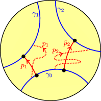
Figure 1. Illustration of the Useful Remark.

Take $3$ distinct non-intersecting geodesics $(\gamma_{i})_{0\leq i\leq 2}$ in the hyperbolic plane $\mathbb{H}^{2}$. Assume that for $i=1,2$ we have a piecewise smooth oriented path $p_{i}$ going from $\gamma_{0}$ to $\gamma_{i}$, intersecting $\gamma_{0}$ and $\gamma_{i}$ only at its endpoints. Therefore, the complement $\mathbb{H}^{2}\setminus(\gamma_{0}\cup\gamma_{i}\cup p_{i})$ has four connected components, that we respectively call north of $\gamma_{i}$, south of $\gamma_{0}$ and east/west of $p_{i}$, following the compass. Assume in addition that $p_{2}$ only visits the east of $p_{1}$, and $p_{1}$ only visits the west of $p_{2}$. Then:

1. the oriented orthogeodesics $\bar{p}_{i}$ from $\gamma_{0}$ to $\gamma_{i}$ are disjoint;

2. $\bar{p}_{2}$ entirely lies east of $\bar{p}_{1}$;

3. $\bar{p}_{1}$ entirely lies west of $\bar{p}_{2}$.

2.1.5. Length of a path or a geodesic

If $\gamma$ is a 1-dimensional Riemannian manifold, we will denote by $\ell(\gamma)$ its length. If now $\gamma$ is a smooth path in a Riemannian manifold $Y$, we will denote by $\ell(\gamma)$ its length in $Y$ (which coincides with its length for the metric on $\gamma$ induced by $Y$). If $\gamma$ is a loop in a hyperbolic surface $Y$, we will denote by $\ell_{Y}(\gamma)$ the minimal length of a representative of the free homotopy class of $\gamma$ (if $\gamma$ is contractible, $\ell_{Y}(\gamma)=0$, otherwise it is the length of the unique geodesic representative of the free homotopy class of $\gamma$). In general, $\ell(\gamma)$ and $\ell_{Y}(\gamma)$ are different, but they are of course equal if $\gamma$ is a closed geodesic in $Y$.

If ${\mathbf{S}}$ is endowed with a hyperbolic structure $Y$, then each component ${\mathbf{c}}_{i}$ of $\mathbf{c}$ is freely homotopic to a periodic geodesic, which is unique if ${\mathbf{c}}_{i}$ is non-contractible, but may be reduced to a point otherwise. We denote $\ell_{Y}({\mathbf{c}})=\sum_{i=1}^{\mathfrak{n}}\ell_{Y}({\mathbf{c}}_{i})$ the total length of a geodesic representative.

2.2. Opening the intersections of ${\mathbf{c}}$

In this paragraph, we explain how to open the self-intersections of ${\mathbf{c}}$ to replace them by bars. Our construction yields a new picture which consists of a simple multi-loop $\beta$ and a collection of bars $B$ with endpoints on $\beta$, replacing the intersections.

Notation 2.12.

Throughout the paper, the letter $r$ stands for the number of self-intersection points of the multi-loop ${\mathbf{c}}$. We identify the set of intersection points of the multi-loop $\mathbf{c}$ with the set $\{1,\ldots,r\}$ by picking an arbitrary numbering.

2.2.1. The construction

If $r=0$ then ${\mathbf{c}}$ is a simple loop and we simply take $\beta={\mathbf{c}}$, and no bars. Now assume $r\geq 1$. Let $a_{1},\ldots,a_{r}$ be the intersection points of $\mathbf{c}$ and $D_{1},\ldots,D_{r}$ be disjoint open disks around them. We can take the disks small enough so that, for each $j$, ${\mathbf{c}}\cap D_{j}$ is the union of two oriented segments $I_{j},I^{\prime}_{j}$ intersecting transversally at $a_{j}$. We open the intersection at each $a_{j}$ and replace the two intersecting segments $I_{j},I^{\prime}_{j}$ by two smooth disjoint segments, joined by a transversal segment $B_{j}$ traversed twice, replacing the intersection. There are two distinct ways to perform this operation, represented in Figure 2(b) and 2(c) respectively.

(a) The initial intersection.

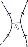
(b) Opening the first way.

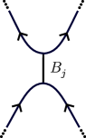
(c) Opening the second way.

Figure 2. Opening an intersection to replace it by a bar, two ways.

Opening all of the intersections (having made an arbitrary choice between the two ways for each intersection) yields a new representative ${\mathbf{c}}^{\mathrm{op}}$ of the homotopy class of ${\mathbf{c}}$, represented in Figure 3. The operation of going from ${\mathbf{c}}$ to the new representative ${\mathbf{c}}^{\mathrm{op}}$ will be referred to as opening the intersections of ${\mathbf{c}}$ (to replace them by bars).

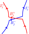
(a) The first way.

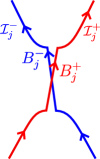
(b) The second way.

Figure 3. A close deformation of the multi-loop ${\mathbf{c}}^{\mathrm{op}}$. Notice that each bar is traversed twice (in the directions we will later denote $B_{j}^{+}$ and $B_{j}^{-}$).

By convention, the bars $B_{j}$ are closed, i.e. contain their endpoints. If $\dot{B_{j}}$ is the open segment, i.e. the segment without its endpoints, we call $\beta$ the connected components of ${\mathbf{c}}^{\mathrm{op}}\setminus(\bigcup_{j=1}^{r}\dot{B_{j}})$. We observe that $\beta$ is a simple multi-loop. The geometric image of ${\mathbf{c}}^{\mathrm{op}}$ is the simple multi-loop $\beta$ joined by the collection of bars $B=(B_{1},\ldots,B_{r})$.

Note that $\beta$ is not necessarily a multi-curve – see Figure 4(b) for an example where one of the components of $\beta$ is contractible. When we later specialise our discussion to the class of multi-loops called generalized eights in §2.3, the family $\beta$ will actually be a multi-curve (see Lemma 2.21).

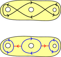
(a) A generalized eight.

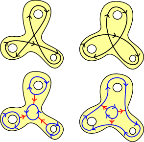
(b) Two non-isotopic representatives of a loop.

Figure 4. An example of the construction for three loops filling a surface of signature $(0,4)$. Here, we opened all the intersections the first way.

Remark 2.13.

The bars are naturally numbered as $(B_{1},\ldots,B_{r})$ thanks to our choice of numbering of the intersection points of $\mathbf{c}$. However, there is no canonical way to number the components of $\beta$ based on our information so far, and because picking a numbering is not very useful for our purposes, we do not do so. We will denote as $\Lambda^{\beta}$ the set of components of $\beta$ (this notation will make more sense after §3.3), so that $\beta=(\beta_{\lambda})_{\lambda\in\Lambda^{\beta}}$.

2.2.2. Orientation of the bars

Let us define orientations $B_{j}^{\pm}$ on the bars $B_{j}$ for $1\leq j\leq r$. The convention will depend on the type of opening.

We first observe that the endpoints of the bars $B_{1},\ldots,B_{r}$ partition the multi-loop $\beta$ into $2r$ segments, reflecting the partition of ${\mathbf{c}}$ into the simple portions defined in Definition 1.21. We will call simple portions of ${\mathbf{c}}^{\mathrm{op}}$ these subsegments of $\beta$. Each simple portion is naturally oriented by the original orientation of ${\mathbf{c}}^{\mathrm{op}}$. Each bar $B_{j}$ touches four (non necessarily distinct) simple portions: two at each endpoint.

We then settle on the following convention, illustrated in Figure 3.

1. In the first way, we choose the orientation $B_{j}^{+}$ of $B_{j}$ such that $B_{j}^{+}$ arrives on the right of the two simple portions touching its terminus $t(B_{j}^{+})$: one of these simple portions originates in $t(B_{j}^{+})$ and the other one terminates in $t(B_{j}^{+})$. Similarly, $B_{j}^{+}$ leaves from the left of the two simple portions touching its origin $o(B_{j}^{+})$; one of them originates in $o(B_{j}^{+})$ and the other one terminates in $o(B_{j}^{+})$. In this case we denote by $B_{j}^{-}$ the opposite orientation of $B_{j}$.

2. In the second way, we choose the orientation $B_{j}^{+}$ of $B_{j}$ such that the two simple portions touching its terminus $t(B_{j}^{+})$ originate in $t(B_{j}^{+})$, and the two simple portions touching its origin $o(B_{j}^{+})$ terminate in $o(B_{j}^{+})$. In this case, we define the orientation $B_{j}^{-}$ to be identical to $B_{j}^{+}$.

2.2.3. Labelling of simple portions

Let us label the simple portions and define a few useful notations. Our most important set of indices will be the set

(2.1) $$\Theta=\{1,\ldots,r\}\times\{+,-\},$$

which will naturally label the simple portions. Indeed, for $(j,\epsilon)\in\Theta$, let $\mathcal{I}_{j}^{\epsilon}$ be the oriented simple portion originating from the terminus of $B_{j}^{\epsilon}$, so that $B^{+}_{j}$ arrives on $\mathcal{I}_{j}^{+}$ from the right at the point $o(\mathcal{I}_{j}^{+})=t(B_{j}^{+})$ and $B^{-}_{j}$ arrives on $\mathcal{I}_{j}^{-}$ from the left at the point $o(\mathcal{I}_{j}^{-})=t(B_{j}^{-})$, as represented in Figure 3.

Remark 2.14.

Note that, out of the four simple portions touching the bar $B_{j}$, only two are labelled $\mathcal{I}_{j}^{\pm}$ by the above convention. The other two simple portions are denoted as $\mathcal{I}_{j^{\prime}}^{\pm}$ for another (possibly equal) integer $j^{\prime}$.

We shall most often refer to the elements of $\Theta$ by the letter $q$, so that if $q=(j,\epsilon)$ is an elements of $\Theta$, then the bar $B_{q}$ stands for $B_{j}^{\epsilon}$, $\mathcal{I}_{q}$ for $\mathcal{I}_{j}^{\epsilon}$, etc.

The signs in $\Theta$ will play an important role throughout the paper.

Notation 2.15.

We define the sign function on $\Theta$ by:

(2.2) $$\forall q=(j,\epsilon)\in\Theta,\quad\operatorname{Sign}(q)=\epsilon.$$

We denote as $\iota:\Theta\rightarrow\Theta$ the involution defined by $\iota(j,\epsilon)=(j,-\epsilon)$.

It will be helpful to relate the elements of $\Theta$ and the components of the multi-loop $\beta$.

Notation 2.16.

For $q\in\Theta$, let $\lambda(q)\in\Lambda^{\beta}$ denote the component of $\beta$ on which $B_{q}$ terminates, i.e. such that the terminus $t(B_{q})$ belongs to the loop $\beta_{\lambda(q)}$.

For $\lambda\in\Lambda^{\beta}$ (i.e. for a component $\beta_{\lambda}$ of the multi-loop $\beta$), we define the set of indices

(2.3) $$\Theta_{t}(\lambda):=\{q\in\Theta:t(B_{q})\in\beta_{\lambda}\}\subseteq\Theta.$$

In other words, this is the set of indices $q\in\Theta$ such that $\lambda(q)=\lambda$, or, equivalently, such that the bar $B_{q}$ terminates on $\beta_{\lambda}$. We extend this notation to any subset $W\subseteq\Lambda^{\beta}$ by letting

(2.4) $$\Theta_{t}(W):=\bigcup_{\lambda\in W}\Theta_{t}(\lambda)=\{q\in\Theta:t(B_{q})\in W\}.$$

Remark 2.17.

We make the key observation that, since the multi-loop $\beta$ is decomposed in the simple portions $\mathcal{I}_{q}$ with $q\in\Theta$, the sets $(\Theta_{t}(\lambda))_{\lambda\in\Lambda^{\beta}}$ generate a partition of $\Theta$:

$$\Theta=\bigsqcup_{\lambda\in\Lambda^{\beta}}\Theta_{t}(\lambda).$$

Remark 2.18.

It will be useful to keep in mind from the construction that each component $\beta_{\lambda}$ of $\beta$ is freely homotopic to an “initial” piecewise smooth curve $\beta_{\lambda,\mathrm{init}}$, included in the original multi-loop ${\mathbf{c}}$, made of smooth segments joining some of the intersection points of $\mathbf{c}$. The partition of $\beta_{\lambda}$ into the union of a collection of segments $(\mathcal{I}_{q})_{q\in\Theta_{t}(\lambda)}$ is inherited from a partition of $\beta_{\lambda,\mathrm{init}}$ into segments $(\mathcal{I}_{q,\mathrm{init}})_{q\in\Theta_{t}(\lambda)}$ which are the simple portions of Definition 1.21.

2.2.4. Diagrams

The result of opening all of the intersections of the multi-loop $\mathbf{c}$ is what we call a diagram.

Definition 2.19.

A diagram $\mathbf{D}$ in $\mathbf{S}$ is the data (modulo isotopy) of a simple multi-loop $\beta$, together with a collection of disjoint bars $B=(B_{1},\ldots,B_{r})$ defined as closed, mutually disjoint segments, having their endpoints in $\beta$ and disjoint from $\beta$ otherwise.

Starting with a multi-loop $\mathbf{c}$ and opening all intersections (either way), we obtain a diagram $\mathbf{D}$, which is said to represent $\mathbf{c}$. Conversely, the multi-loop $\mathbf{c}$ is said to stem from $\mathbf{D}$ if $\mathbf{D}$ represents $\mathbf{c}$.

Different representatives of the same homotopy class may give rise to non-isotopic diagrams: see Figure 4(b). The paper by Graaf and Schrijver [7] precisely describes when two multi-loops can be homotopic without being isotopic: this may happen if and only if one can be sent to the other by an isotopy followed by a finite succession of Reidemeister moves of type III.

2.2.5. First v.s. second way

Throughout this article, we will be in particular interested in the case when we open all of the intersections the first way. We denote by $\mathbf{D}^{(1)}$ the diagram obtained by opening all intersections the first way. One possible reason for preferring the first way is the fact that the multi-loop $\beta$ then inherits a global orientation that fits with the orientation of the simple portions $(\mathcal{I}_{q})_{q\in\Theta}$, in other words with the initial orientation of ${\mathbf{c}}$. If we open the intersections the second way, the orientations of the simple portions $(\mathcal{I}_{q})_{q\in\Theta}$ do not fit into a global orientation of $\beta$, which is not a problem, but can sometimes be slightly cumbersome in terms of notations.

Unless explicitely stated, for the sake of simplicity, we invite the reader to consider that the construction above has been done by opening every intersection the first way. However, many of our results, notably our change of variable presented in §3, hold for whichever choice of opening is made – different openings yielding different interesting results. We will be careful to point out the few places where the choice of opening actually does matter.

2.3. Generalized eights

We introduce a class of multi-loops, called generalized eights, on which we focus attention for most of the paper. Their name comes from the fact that they are generalizations of the basic figure-eight loop, the loop with exactly one self-intersection ($r=1$).

Definition 2.20.

Let $\mathcal{N}$ be a regular neighbourhood of ${\mathbf{c}}$ in ${\mathbf{S}}$. We say that ${\mathbf{c}}$ is a generalized eight if no connected components of $\partial\mathcal{N}$ is contractible in ${\mathbf{S}}$.

This definition has the following consequence on the surface $\mathbf{S}$ and the multi-loop $\beta$.

Lemma 2.21.

If $\mathbf{c}$ is a generalized eight, then $\chi(\mathbf{S})=r$ and $\beta$ is a multi-curve.

Proof.

Let $\mathcal{N}$ be a regular neighbourhood of $\mathbf{c}$ in $\mathbf{S}$. Since $\mathbf{c}$ fills $\mathbf{S}$ and no boundary component of $\mathcal{N}$ is contractible, $\mathbf{S}\setminus\mathcal{N}$ is a union of cylinders, and hence $\chi(\mathbf{S})=\chi(\mathcal{N})$. We then conclude by observing that the regular neighbourhood $\mathcal{N}$ retracts on the $4$-regular graph with vertices the $r$ intersections points of $\mathbf{c}$, and edges its $2r$ simple portions, of Euler characteristic $r-2r=-r$.

The definition of generalized eight directly implies that none of the components of $\beta$ is contractible. To prove that $\beta_{i}$ cannot be freely homotopic to $\beta_{j}$ or its inverse for $i\neq j$ two components of $\beta$, we remark that if $\beta_{i}$ is freely homotopic to $\beta_{j}$ or its inverse, then there is a cylinder in ${\mathbf{S}}$ bordered by $\beta_{i}$ and $\beta_{j}$. This cylinder may contain in its interior other components $\beta_{k}$ homotopic to $\beta_{i}^{\pm 1}$. We pick $k$ such that the cylinder $C$ bordered by $\beta_{i}$ and $\beta_{k}$ does not contain in its interior any other component of the multi-loop $\beta$. Because ${\mathbf{c}}$ fills ${\mathbf{S}}$, the cylinder $C$ must contain bars $B_{l}$ going from $\beta_{i}$ to $\beta_{k}$. These bars, together with $\beta_{i}$ and $\beta_{k}$, cut $C$ into connected components homeomorphic to disks, contradicting the fact that $\partial\mathcal{N}$ does not have contractible components. ∎

Remark 2.22.

If $\mathbf{c}$ is a generalized eight, Reidemeister moves of type III are not possible and hence any multi-loop homotopic to $\mathbf{c}$ is also isotopic. As a consequence, the diagram $\mathbf{D}^{(1)}$ obtained by opening the intersections the first way is uniquely defined up to isotopy.

2.4. Removing bars and intersections

We define two ways of removing a bar from a diagram: either by just deleting it (we call this the first way of removing a bar), or the second way, shown on Figure 5(a).

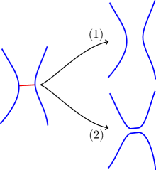
(a) A bar in a diagram.

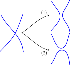
(b) An intersection on a multi-loop.

Figure 5. The two ways of removing a bar on a diagram or an intersection point on a multi-loop.

If the diagram was obtained by opening all intersections of a multi-loop ${\mathbf{c}}$, removing a bar corresponds to removing an intersection from ${\mathbf{c}}$. Correspondingly, there are two ways to remove an intersection from ${\mathbf{c}}$ (the first and the second way), shown on Figure 5(b).

We make the following straightforward observation, which will enable us to argue by induction on $r$ in the proof of Theorem 3.11.

Lemma 2.23.

If ${\mathbf{c}}$ is a generalized eight, the multi-loop ${\mathbf{c}}^{\prime}$ obtained by removing an intersection point is still a generalized eight, filling a surface of absolute Euler characteristic $r-1$.

Note that the number of components of the multi-loop ${\mathbf{c}}^{\prime}$ is, a priori, different from the number of components of $\mathbf{c}$; this is one of the motivations for studying multi-loops instead of mere loops.

2.5. Reconstitution of ${\mathbf{c}}^{\mathrm{op}}$ and relabelling of $\Theta$

Let us explain how to retrieve the multi-loop $\mathbf{c}$ from the diagram, and define some convenient notations to express the representant ${\mathbf{c}}^{\mathrm{op}}$ of the homotopy class of $\mathbf{c}$ in terms of a succession of bars and simple portions.

2.5.1. Cycle-decomposition and rewriting of ${\mathbf{c}}^{\mathrm{op}}$

For $q\in\Theta$, we define

(2.5) $$p(q):=B_{q}\mathord{\mathchoice{\,\vbox{\hbox{\scalebox{0.5}{$\displaystyle\bullet$}}}\,}{\,\vbox{\hbox{\scalebox{0.5}{$\textstyle\bullet$}}}\,}{\,\vbox{\hbox{\scalebox{0.5}{$\scriptstyle\bullet$}}}\,}{\,\vbox{\hbox{\scalebox{0.5}{$\scriptscriptstyle\bullet$}}}\,}}\mathcal{I}_{q}$$

to be the concatenation of the oriented segments $B_{q}$ and $\mathcal{I}_{q}$ (which do, by definition, connect). The representative ${\mathbf{c}}^{\mathrm{op}}$ of the homotopy class of ${\mathbf{c}}$ is the concatenation of the $2r$ paths $p(q)$ for $q\in\Theta$. More precisely, there is a unique permutation $\sigma$ of the set $\Theta$, decomposed into $\mathfrak{n}$ disjoint cycles $\sigma=\prod_{i=1}^{\mathfrak{n}}(q_{1}^{i}\,q_{2}^{i}\,\ldots\,q_{n_{i}}^{i})$ such that, for all $i\in\{1,\ldots,\mathfrak{n}\}$, the $i$th component ${\mathbf{c}}^{\mathrm{op}}_{i}$ of ${\mathbf{c}}^{\mathrm{op}}$ coincides with the concatenation

(2.6) $${\mathbf{c}}^{\mathrm{op}}_{i}=p(q_{1}^{i})\mathord{\mathchoice{\,\vbox{\hbox{\scalebox{0.5}{$\displaystyle\bullet$}}}\,}{\,\vbox{\hbox{\scalebox{0.5}{$\textstyle\bullet$}}}\,}{\,\vbox{\hbox{\scalebox{0.5}{$\scriptstyle\bullet$}}}\,}{\,\vbox{\hbox{\scalebox{0.5}{$\scriptscriptstyle\bullet$}}}\,}}p(q_{2}^{i})\mathord{\mathchoice{\,\vbox{\hbox{\scalebox{0.5}{$\displaystyle\bullet$}}}\,}{\,\vbox{\hbox{\scalebox{0.5}{$\textstyle\bullet$}}}\,}{\,\vbox{\hbox{\scalebox{0.5}{$\scriptstyle\bullet$}}}\,}{\,\vbox{\hbox{\scalebox{0.5}{$\scriptscriptstyle\bullet$}}}\,}}\ldots\mathord{\mathchoice{\,\vbox{\hbox{\scalebox{0.5}{$\displaystyle\bullet$}}}\,}{\,\vbox{\hbox{\scalebox{0.5}{$\textstyle\bullet$}}}\,}{\,\vbox{\hbox{\scalebox{0.5}{$\scriptstyle\bullet$}}}\,}{\,\vbox{\hbox{\scalebox{0.5}{$\scriptscriptstyle\bullet$}}}\,}}p(q_{n_{i}}^{i})$$

(or a circular permutation thereof).

The length of the $i$-th cycle is denoted as $n_{i}$, and we have $\sum_{i=1}^{\mathfrak{n}}n_{i}=2r$. Because of the invariance of the free homotopy class of (2.6) under circular permutation, it is convenient to consider that the elements $q_{k}^{i}=(j^{i}_{k},\epsilon^{i}_{k})\in\Theta$ are numbered by $k\in\mathbb{Z}_{n_{i}}$ where $\mathbb{Z}_{n_{i}}:=\mathbb{Z}\diagup n_{i}\mathbb{Z}$.

Remark 2.24.

By construction, we have the following orientation rules in (2.6), see Figure 3:

• if $\epsilon^{i}_{k}=+$ then $B_{q^{i}_{k}}$ arrives at $\mathcal{I}_{q^{i}_{k}}$ from the right and leaves from $\mathcal{I}_{q^{i}_{k-1}}$ from the left;

• otherwise, $B_{q^{i}_{k}}$ arrives at $\mathcal{I}_{q^{i}_{k}}$ from the left and leaves from $\mathcal{I}_{q^{i}_{k-1}}$ from the right.

2.5.2. Re-labelling of $\Theta$

For $q\in\Theta$, let $\operatorname{Comp}(q)=i\in\{1,\ldots,\mathfrak{n}\}$ be the label of the component ${\mathbf{c}}_{i}$ of $\mathbf{c}$ in which $q$ appears in the decomposition (2.6). We set

$$\Theta^{i}=\{q\in\Theta,\operatorname{Comp}(q)=i\}.$$

Then, for any $q\in\Theta^{i}$, we can write using the permutation $\sigma$:

(2.7) $${\mathbf{c}}^{\mathrm{op}}_{i}=p(q)\mathord{\mathchoice{\,\vbox{\hbox{\scalebox{0.5}{$\displaystyle\bullet$}}}\,}{\,\vbox{\hbox{\scalebox{0.5}{$\textstyle\bullet$}}}\,}{\,\vbox{\hbox{\scalebox{0.5}{$\scriptstyle\bullet$}}}\,}{\,\vbox{\hbox{\scalebox{0.5}{$\scriptscriptstyle\bullet$}}}\,}}p(\sigma q)\mathord{\mathchoice{\,\vbox{\hbox{\scalebox{0.5}{$\displaystyle\bullet$}}}\,}{\,\vbox{\hbox{\scalebox{0.5}{$\textstyle\bullet$}}}\,}{\,\vbox{\hbox{\scalebox{0.5}{$\scriptstyle\bullet$}}}\,}{\,\vbox{\hbox{\scalebox{0.5}{$\scriptscriptstyle\bullet$}}}\,}}p(\sigma^{2}q)\mathord{\mathchoice{\,\vbox{\hbox{\scalebox{0.5}{$\displaystyle\bullet$}}}\,}{\,\vbox{\hbox{\scalebox{0.5}{$\textstyle\bullet$}}}\,}{\,\vbox{\hbox{\scalebox{0.5}{$\scriptstyle\bullet$}}}\,}{\,\vbox{\hbox{\scalebox{0.5}{$\scriptscriptstyle\bullet$}}}\,}}\ldots\mathord{\mathchoice{\,\vbox{\hbox{\scalebox{0.5}{$\displaystyle\bullet$}}}\,}{\,\vbox{\hbox{\scalebox{0.5}{$\textstyle\bullet$}}}\,}{\,\vbox{\hbox{\scalebox{0.5}{$\scriptstyle\bullet$}}}\,}{\,\vbox{\hbox{\scalebox{0.5}{$\scriptscriptstyle\bullet$}}}\,}}p(\sigma^{n_{i}-1}q).$$

We now consider the set

$$\Theta^{\prime}=\bigsqcup_{i=1}^{\mathfrak{n}}\mathbb{Z}_{n_{i}}=\{(i,k),i\in\{1,\ldots,\mathfrak{n}\},k\in\mathbb{Z}_{n_{i}}\}.$$

The map

(2.8) $$\phi:\begin{cases}\Theta^{\prime}&\rightarrow\Theta\\ (i,k)&\mapsto q^{i}_{k}=(j^{i}_{k},\epsilon^{i}_{k})\end{cases}$$

is a bijection, and the cyclic ordering of $\mathbb{Z}_{n_{i}}$ is compatible with the cycling ordering of $q^{i}_{k}$ in the path (2.6). We shall identify $\Theta$ with $\Theta^{\prime}$ through the map $\phi$, thus writing $(i,k)$ for $1\leq i\leq\mathfrak{n}$, $k\in\mathbb{Z}_{n_{i}}$ to enumerate the elements of $\Theta$. Doing so, $\Theta^{i}$ can be identified with $\{(i,k),k\in\mathbb{Z}_{n_{i}}\}$, that is to say, with $\mathbb{Z}_{n_{i}}$. After this identification, the permutation $\sigma$ is given by $(i,k)\mapsto(i,k+1)$.

2.5.3. Periodic extensions

Similarly define

$${\mathbf{\Theta}}=\bigsqcup_{i=1}^{\mathfrak{n}}\mathbb{Z}=\{(i,k),i\in\{1,\ldots,\mathfrak{n}\},k\in\mathbb{Z}\}=\bigsqcup_{i=1}^{\mathfrak{n}}{\mathbf{\Theta}}^{i},$$

where ${\mathbf{\Theta}}^{i}=\{(i,k),k\in\mathbb{Z}\}$. When needed, the sequence $(i,k)\mapsto q^{i}_{k}$ can also be defined for $(i,k)\in{\mathbf{\Theta}}$ by pre-composing with the projection map $\mathbb{Z}\rightarrow\mathbb{Z}_{n_{i}}$. In accordance with the previous discussion, we will denote $\sigma:{\mathbf{\Theta}}\rightarrow{\mathbf{\Theta}}$ the shift map $(i,k)\mapsto(i,k+1)$.

2.6. U-turns and crossings

The following definition will be useful to our analysis.

Definition 2.25.

For $q\in\Theta$, we say that $q$ is a crossing index if $\operatorname{Sign}(q)\operatorname{Sign}(\sigma q)=+1$, and a U-turn index otherwise. We denote by $\mathcal{C}\subseteq\Theta$ the set of crossing indices and by $\mathcal{U}\subseteq\Theta$ the set of U-turn indices. If $\Theta=\mathcal{U}$, we say that we are in the purely non-crossing case.

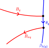
(a) U-turn.

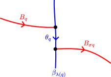
(b) Crossing.

Figure 6. A U-turn v.s. crossing index (here $\operatorname{Sign}(q)=+$).

The terminology is motivated by the fact that if $q$ is a crossing index, then to go from $B_{q}$ to $B_{\sigma q}$ we have to cross the component $\beta_{\lambda(q)}$ of $\beta$, while in the other case, we make a U-turn when arriving at $\beta_{\lambda(q)}$. See Figure 6.

3. Coordinate system adapted to a generalized eight

We assume until §11 that the multi-loop ${\mathbf{c}}$ is a generalized eight filling a surface ${\mathbf{S}}$. We open the intersections of ${\mathbf{c}}$ by the procedure defined in the previous section (in this section, we allow every intersection to be opened in the first or second way). By hypothesis, the simple multi-loop $\beta$ is a multi-curve. Let us show how the bars $B_{1},\ldots,B_{r}$ and the simple portions $(\mathcal{I}_{q})_{q\in\Theta}$ can be used to define new coordinates on the Teichmüller space $\mathcal{T}^{*}_{g_{\mathbf{S}},n_{\mathbf{S}}}$ of marked hyperbolic metrics on $\mathbf{S}$, well-adapted to expressing the length function of ${\mathbf{c}}$.

First, we notice that the dimension of $\mathcal{T}_{g_{\mathbf{S}},n_{\mathbf{S}}}^{*}$ is equal to $6g_{\mathbf{S}}-6+3n_{\mathbf{S}}=3\chi(\mathbf{S})$. We proved in Lemma 2.21 that, for a generalized eight, $\chi(\mathbf{S})=r$. As a consequence, the dimension of the Teichmüller space $\mathcal{T}^{*}_{g_{\mathbf{S}},n_{\mathbf{S}}}$ is $3r$, so this is the number of coordinates we expect to need to describe a point on $\mathcal{T}_{g_{\mathbf{S}},n_{\mathbf{S}}}^{*}$.

3.1. Coordinates $\vec{L}=(L_{1},\ldots,L_{r})$ and $\vec{\theta}=(\theta_{1}^{\pm},\ldots,\theta_{r}^{\pm})$ on the Teichmüller space

Consider a point $Y\in\mathcal{T}^{*}_{g_{\mathbf{S}},n_{\mathbf{S}}}$, i.e. a compact hyperbolic metric on $\mathbf{S}$. As explained in Remark 2.8, we take a representative of $Y$ in the Teichmüller space such that the multi-curve $\beta$ is a simple multi-geodesic.

For $q\in\Theta$, we replace the bar $B_{q}$ by the representative $\overline{B}_{q}$ of minimal length in its homotopy class with endpoints gliding on $\beta$. While the endpoints $t(B_{q})$ glide to the new endpoints $t(\overline{B}_{q})$ along $\beta$, it is important to note that the segments $\mathcal{I}_{q}$ glide to new segments $\overline{\mathcal{I}}_{q}$ of $\beta_{\lambda(q)}$. Although the original segments $\mathcal{I}_{q}$ were positively oriented along $\beta_{\lambda(q)}$, it can happen that $\overline{\mathcal{I}}_{q}$ goes in the reverse direction, or that $\overline{\mathcal{I}}_{q}$ wraps an arbitrary number of times around $\beta_{\lambda(q)}$.

We are now ready to define our new coordinates on the Teichmüller space $\mathcal{T}_{g_{\mathbf{S}},n_{\mathbf{S}}}^{*}$.

Definition 3.1 (Coordinates $(\vec{L},\vec{\theta})$).

Let $Y\in\mathcal{T}_{g_{\mathbf{S}},n_{\mathbf{S}}}^{*}$.

1. For $j\in\{1,\ldots,r\}$, we denote by $L_{j}=L_{j}(Y)$ the (positive) length of the orthogeodesic $\overline{B}_{j}$. We write $\vec{L}=(L_{1},\ldots,L_{r})$.

2. For $q\in\Theta$, we denote by $\theta_{q}=\theta_{q}(Y)$ the algebraic length of $\overline{\mathcal{I}}_{q}$: positive if it goes in the same direction as $\mathcal{I}_{q}$, negative otherwise. We write $\vec{\theta}=(\theta_{q})_{q\in\Theta}$.

Figure 7. An example of coordinates $(\vec{L},\vec{\theta})$ in a case when $r=2$. We have additionally represented the pair of pants decomposition constructed in §3.2 as dashed curves (here, $\#\Lambda^{\beta}=3$ and $\#\Lambda^{\Gamma}=2$).

Remark 3.2 (Crossing and U-turn variables).

If $q\in\mathcal{C}$ is a crossing index, then we say that $\theta_{q}$ is a crossing variable; if $q\in\mathcal{U}$ is a U-turn variable, then we say that $\theta_{q}$ is a U-turn variable. By the Useful Remark (Remark 2.11), U-turn variables are always positive: if $q\in\mathcal{U}$, then $\theta_{q}\geq 0$. Thus, the discussion concerning U-turn variables is a little simpler than for crossing variables.

Notation 3.3.

It will often be convenient to use the notation $L(q)=L_{j}$ for $q=(j,\epsilon)\in\Theta$ (note that $L(q)$ does not depend on the sign component of $q$). We will also benefit from introducing $\epsilon L(q):=\operatorname{Sign}(q)L(q)$. The vector $(\epsilon L(q))_{q\in\Theta}$ then contains each length $L_{j}$ exactly twice, once positively and once negatively. This corresponds to the fact that each bar is explored exactly twice when going along ${\mathbf{c}}^{\mathrm{op}}$, following its two orientations, as illustrated in Figure 3.

We can already note that $(\vec{L},\vec{\theta})$ belongs to $\mathbb{R}_{>0}^{r}\times\mathbb{R}^{\Theta}\subset\mathbb{R}^{3r}$, a space of same dimension as the Teichmüller space $\mathcal{T}^{*}_{g_{\mathbf{S}},n_{\mathbf{S}}}$. The remainder of this section is devoted to proving that $(\vec{L},\vec{\theta})$ is a coordinate system on $\mathcal{T}^{*}_{g_{\mathbf{S}},n_{\mathbf{S}}}$, finding the expression of the Weil–Petersson measure in these coordinates, and describing its range.

We do not start from scratch, but use the fact that the expression for the Weil–Petersson measure is already known in Fenchel–Nielsen coordinates, thanks to Wolpert’s theorem [14]. In order to apply Wolpert’s result, we use an auxiliary decomposition of ${\mathbf{S}}$ into pairs of pants, determined by the multi-curve $\beta$ and the bars $B_{1},\ldots,B_{r}$. We find relations between the Fenchel–Nielsen coordinates and the parameters $(\vec{L},\vec{\theta})$, and calculate the determinant.

Remark 3.4.

This approach seems a bit artificial, and it would be interesting to study directly the Weil–Petersson measure in coordinates $(\vec{L},\vec{\theta})$, without resorting to an auxiliary system of Fenchel–Nielsen coordinates.

3.2. Decomposition into pairs of pants

Using the multi-curve $\beta$ and the bars $B_{1},\ldots,B_{r}$, we define a decomposition of ${\mathbf{S}}$ into pairs of pants (3-holed spheres) that will serve as an auxiliary tool in several places.

3.2.1. Pair of pants determined by two simple curves joined by a segment

Let $(C_{+},C_{-})$ be a multi-curve on $\mathbf{S}$, and $B$ be a simple segment going from $C_{-}$ to $C_{+}$, not intersecting $C_{-}\cup C_{+}$ except at its endpoints. The topological pair of pants determined by $C_{-}$, $C_{+}$ and $B$ is defined as a one-sided regular neighbourhood of $C_{-}\cup C_{+}\cup B$; that is to say, a regular neighbourhood $\mathcal{N}$ of $C_{-}\cup C_{+}\cup B$, from which we remove the cylinders bordered by one of the curves $C_{\pm}$ and one component of $\partial\mathcal{N}$.

This also applies when $C=C_{+}=C_{-}$ as soon as $B$ is not homotopically trivial with gliding endpoints along $C$. We have either a pair of pants if $B$ leaves and arrives on the same side of $C$, or a once-holed torus otherwise.

The three cases are shown in Figure 8.

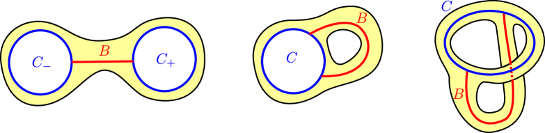
Figure 8. The three possible pairs of pants (or once-holed tori) determined by two simple curves joined by a segment.

3.2.2. Construction of the pair of pants decomposition

The (arbitrary) numbering of $B_{1},\ldots,B_{r}$ determines a decomposition $({\mathbf{P}}_{1},\ldots,{\mathbf{P}}_{r})$ of ${\mathbf{S}}$ into connected surfaces of Euler characteristic $-1$, defined inductively below. This decomposition is non-canonical, as it depends on the numbering of the bars $B_{1},\ldots,B_{r}$.

The construction provides us with an increasing family of multi-curves $\Sigma_{0}\subset\Sigma_{1}\subset\ldots\subset\Sigma_{r}$, and an increasing family of surfaces ${\mathbf{S}}_{j}={\mathbf{S}}_{j-1}\cup{\mathbf{P}}_{j}$ for $1\leq j\leq r$. It will also produce an auxiliary family of sets $\widetilde{{\mathbf{S}}}_{j}$.

• To initiate, we let ${\mathbf{S}}_{0}=\emptyset$ and $\widetilde{{\mathbf{S}}}_{0}=\Sigma_{0}$ be the multi-curve $\beta$.

• Let $j\in\{1,\ldots,r\}$. The intersection of the $j$-th bar $B_{j}$ with $\widetilde{{\mathbf{S}}}_{j-1}$ is the union of two non-empty closed segments $I_{+}$, $I_{-}$ (possibly reduced to single points) containing the endpoints of $B_{j}$. The complement of $I_{+}\cup I_{-}$ in $B_{j}$ is a non-empty sub-segment $B^{\prime}_{j}$ of $B_{j}$ which meets one or two components of $\partial\widetilde{{\mathbf{S}}}_{j-1}$ at its endpoints; call $C_{+},C_{-}$ these components. We let ${\mathbf{P}}_{j}$ be the pair of pants determined by $B^{\prime}_{j}$, $C_{+}$ and $C_{-}$.

• We then let $\Sigma_{j}=\Sigma_{j-1}\cup\partial{\mathbf{P}}_{j}$ (it is a multi-curve), $\widetilde{{\mathbf{S}}}_{j}=\widetilde{{\mathbf{S}}}_{j-1}\cup{\mathbf{P}}_{j}$ (the disjoint union of a surface and a multi-curve) and ${\mathbf{S}}_{j}={\mathbf{S}}_{j-1}\cup{\mathbf{P}}_{j}={\mathbf{P}}_{1}\cup\ldots\cup{\mathbf{P}}_{j}$ (a bona-fide surface). They are related by $\widetilde{{\mathbf{S}}}_{j}={\mathbf{S}}_{j}\cup\beta$.

By an argument similar to Remark 2.21, because $\mathbf{c}$ is a generalized eight, the boundary of each pair of pants $\mathbf{P}_{j}$ is a multi-curve in $\mathbf{S}$. The construction finishes for $j=r$, and we have $\widetilde{{\mathbf{S}}}_{r}={{\mathbf{S}}}_{r}={\mathbf{S}}$, because the multi-loop $\mathbf{c}$ fills the surface $\mathbf{S}$.

Remark 3.5.

For each $j$, the surface $\mathbf{S}_{j}$ is filled by the multi-loop $\mathbf{c}^{\prime}$ obtained by removing the intersections $j+1,\ldots,r$ from $\mathbf{c}$ the first way, according to the procedure described in §2.4. The pairs of pants decomposition $\mathbf{P}_{1},\ldots,\mathbf{P}_{j}$ associated to the multi-loops $\mathbf{c}$ and $\mathbf{c}^{\prime}$ are the same.

3.2.3. Reduction to Case (a) and (b)

We shall assume (without loss of generality) that the numbering of $B_{1},\ldots,B_{r}$ is such that the first bars $B_{1},\ldots,B_{r_{0}}$ are in the third situation of Figure 8 (that is, depart and arrive on one unique component of $\beta$, on opposite sides) and the remaining $B_{r_{0}+1},\ldots,B_{r}$, either join two different components of $\beta$, or depart and arrive on one component of $\beta$ on the same side, or leave from a component of $\beta$ already touched by $B_{1},\ldots,B_{r_{0}}$. Then, ${\mathbf{P}}_{1},\ldots,{\mathbf{P}}_{r_{0}}$ are disjoint once-holed tori, and ${\mathbf{P}}_{r_{0}+1},\ldots,{\mathbf{P}}_{r}$ are bona fide pairs of pants falling into one of the first two cases of Figure 8.

As a consequence, for $j>r_{0}$, there are only two possible scenarios that can happen at the $j$-th step in the construction of the pair of pants decomposition, which we shall call Case (a) and Case (b); they are represented in Figure 9.

1. $C_{-}$ and $C_{+}$ are distinct (i.e. the bar $B_{j}^{\prime}$ has endpoints on different components of $\partial\tilde{\mathbf{S}}_{j}$), and hence $\mathbf{S}_{j}$ has one more genus and one less boundary component than $\mathbf{S}_{j-1}$.

2. $C_{-}=C_{+}$ (i.e. the bar $B_{j}^{\prime}$ has endpoints on one unique component of $\partial\tilde{\mathbf{S}}_{j}$), and hence $\mathbf{S}_{j}$ has one more boundary component than $\mathbf{S}_{j-1}$, and the same genus.

We will refer to these two cases in proofs by induction.

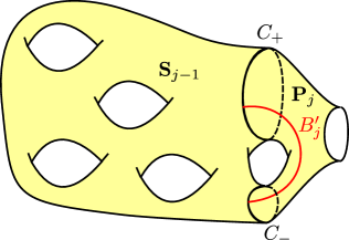
(a) Case (a).

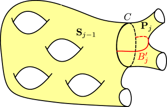
(b) Case (b).

Figure 9. The two possible scenarios when constructing $\mathbf{P}_{j}$.

3.3. Set of boundary components of the pair of pants decomposition

3.3.1. Definition

Let us denote as $\Gamma=(\Gamma_{\lambda})_{\lambda\in\Lambda}$ the multi-curve $\Sigma_{r}$ in the construction above, i.e. the multi-curve obtained by taking the boundary of the pair of pants decomposition $\textbf{P}_{1},\ldots,\mathbf{P}_{r}$ of $\mathbf{S}$. It is indexed by a set $\Lambda$ with $3g_{\mathbf{S}}-3+2n_{\mathbf{S}}$ elements.

Remark 3.6.

The construction above provides a special representative of the homotopy class of each boundary component $\Gamma_{\lambda}$, as a simple piecewise smooth curve made of a concatenation of bars $\overline{B}_{q}$ and simple portions of $\beta$ (see the forthcoming Figure 20 for an example). More precisely, we will show later that the $\Gamma_{\lambda}$ are what we call polygonal curves, as defined in Definition 8.1. This property will play a key role in §4.4 and §8.

Remark 3.7.

Extending Remark 2.18, it will also be convenient to keep in mind that each boundary component $\Gamma_{\lambda}$ is freely homotopic to a piecewise smooth curve $\Gamma_{\lambda,\mathrm{init}}$, included in the original ${\mathbf{c}}$, made of smooth segments joining some of the intersection points of $\mathbf{c}$.

3.3.2. Partitions of $\Lambda$

Some of the elements of $\Lambda$ are the boundary components of $\mathbf{S}$ – we denote as $\Lambda_{\mathrm{BC}}$ this set, which is in natural bijection with $\partial\mathbf{S}=\{1,\ldots,n_{\mathbf{S}}\}$. The other elements are inner curves, and we denote this set as $\Lambda_{\mathrm{in}}:=\Lambda\setminus\Lambda_{\mathrm{BC}}$. We have $\#\Lambda_{\mathrm{in}}=3g_{\mathbf{S}}-3+n_{\mathbf{S}}$.

We notice that the multi-curve $\beta$ is part of this pair of pants decomposition (because $\beta=\Sigma_{0}\subset\Sigma_{r}$). To reflect this, we define $\Lambda^{\beta}\subseteq\Lambda$ to be the set of components of $\Gamma$ which are also a component of the multi-curve $\beta$. This motivates the writing of the multi-curve $\beta$ as $(\beta_{\lambda})_{\lambda\in\Lambda^{\beta}}$ introduced before, where $\Gamma_{\lambda}=\beta_{\lambda}$ for $\beta\in\Lambda^{\beta}$.

The components of $\Gamma$ which are not part of the multi-loop $\beta$, and have therefore been created in the process of creating Fenchel–Nielsen parameters, will be denoted as $\Lambda^{\Gamma}:=\Lambda\setminus\Lambda^{\beta}$. The partition $\Lambda=\Lambda_{\mathrm{BC}}\sqcup\Lambda_{\mathrm{in}}$ between boundary/inner components naturally induces two partitions of $\Lambda^{\beta}$ and $\Lambda^{\Gamma}$, defined by

$$\Lambda_{\mathrm{BC}}^{\beta}:=\Lambda_{\mathrm{BC}}\cap\Lambda^{\beta} \Lambda_{\mathrm{BC}}^{\Gamma}:=\Lambda_{\mathrm{BC}}\cap\Lambda^{\Gamma}$$

$$\Lambda_{\mathrm{in}}^{\beta}:=\Lambda_{\mathrm{in}}\cap\Lambda^{\beta} \Lambda_{\mathrm{in}}^{\Gamma}:=\Lambda_{\mathrm{in}}\cap\Lambda^{\Gamma}.$$

3.3.3. Order on $\Lambda$

We do not fix a numbering of the set $\Lambda$. However, it will be convenient to equip $\Lambda$ with an order relation in the following way.

Definition 3.8.

For $\lambda\in\Lambda$, we denote as $\mathrm{step}(\lambda)$ the step of the induction when the component $\Gamma_{\lambda}$ is created, i.e.

$$\mathrm{step}(\lambda):=\min\{j\in\{1,\ldots,r\}:\,\Gamma_{\lambda}\text{ is a boundary component of }\mathbf{P}_{j}\}.$$

This induces an order on $\Lambda$, defined by writing, for $\lambda,\lambda^{\prime}\in\Lambda$,

$$\lambda<\lambda^{\prime}\Leftrightarrow\mathrm{step}(\lambda)<\mathrm{step}(\lambda^{\prime}).$$

The relation $\lambda<\lambda^{\prime}$ simply mean that $\Gamma_{\lambda}$ appeared earlier than $\Gamma_{\lambda^{\prime}}$ in our recursive construction of the pants decomposition.

Remark 3.9.

This order is strongly connected (for any $\lambda$, $\lambda^{\prime}$, either $\lambda\leq\lambda^{\prime}$ or $\lambda^{\prime}\leq\lambda$) but a priori not anti-symmetric (there would typically be distinct elements $\lambda\neq\lambda^{\prime}$ with $\mathrm{step}(\lambda)=\mathrm{step}(\lambda^{\prime})$, since we often create several boundary components at a given step of the induction).

Remark 3.10.

In the proof by induction of §3.4.4, it will be convenient to assume that the arbitrary choice of the numbering $\{1,\ldots,n_{\mathbf{S}}\}$ of the boundary of $\mathbf{S}$ has been made so that the function $\lambda\mapsto\mathrm{step}(\lambda)$ is non-decreasing as a function of $\lambda\in\Lambda_{\mathrm{BC}}=\{1,\ldots,n_{\mathbf{S}}\}$, i.e. for every $i<j$ in $\{1,\ldots,n_{\mathbf{S}}\}$, the $j$-th boundary component of $\partial\mathbf{S}$ appears after (or at the same time as) the $i$-th boundary component in the construction of the pair of pants decomposition. In particular, the new components appearing in the last step, when we add the final pair of pants $\mathbf{P}_{r}$, are labelled $n_{\mathbf{S}}$ in Case (a), or $n_{\mathbf{S}}$ and $n_{\mathbf{S}}-1$ in Case (b).

3.4. Expression of the Weil–Petersson measure

We are now ready to state and prove our new expression for the Weil–Petersson measure in the coordinates $(\vec{L},\vec{\theta})$.

3.4.1. Expression in Fenchel–Nielsen coordinates

For given boundary lengths $\mathbf{x}$, once a decomposition of $\mathbf{S}$ into pairs of pants ${\mathbf{P}}_{1},\ldots,{\mathbf{P}}_{r}$ is given, it is standard to consider Fenchel–Nielsen coordinates $(y_{\lambda},\alpha_{\lambda})_{\lambda\in\Lambda_{\mathrm{in}}}$ on $\mathcal{T}_{g_{\mathbf{S}},n_{\mathbf{S}}}(\mathbf{x})$. The coordinates $y_{\lambda}$ are the lengths $\ell_{Y}(\Gamma_{\lambda})$ of the closed geodesics homotopic to $\Gamma_{\lambda}$ for the metric $Y$. The coordinates $\alpha_{\lambda}$ are twist parameters, defined up to translation. We will explain in the proof of Theorem 3.11 how to adequately choose the origin of twist parameters in relation with the multi-loop ${\mathbf{c}}$ that we want to study. By work of Wolpert [14], we know that

(3.1) $$\,\mathrm{d}\mathrm{Vol}^{\mathrm{WP}}_{g_{\mathbf{S}},n_{\mathbf{S}},\mathbf{x}}(Y)=\prod_{\lambda\in\Lambda_{\mathrm{in}}}\,\mathrm{d}y_{\lambda}\,\mathrm{d}\alpha_{\lambda}.$$

To obtain coordinates on $\mathcal{T}^{*}_{g_{\mathbf{S}},n_{\mathbf{S}}}$, we simply multiply this by the Lebesgue measure for the length parameters $\mathbf{x}=(x_{1},\ldots,x_{n_{\mathbf{S}}})$, in other words the collection of $y_{\lambda}$ for $\lambda\in\Lambda_{\mathrm{BC}}$. Since $\Lambda=\Lambda_{\mathrm{in}}\cup\Lambda_{\mathrm{BC}}$, we obtain the expression

(3.2) $$\,\mathrm{d}\mathrm{Vol}^{\mathrm{WP}}_{g_{\mathbf{S}},n_{\mathbf{S}}}(\mathbf{x},Y)=\prod_{\lambda\in\Lambda}\,\mathrm{d}y_{\lambda}\prod_{\lambda\in\Lambda_{\mathrm{in}}}\,\mathrm{d}\alpha_{\lambda}.$$

3.4.2. Main statement

We shall prove the following.

Theorem 3.11.

Let $\mathbf{c}$ be a generalized eight. For any diagram $\mathbf{D}$ representing $\mathbf{c}$, the map

(3.3) $$\begin{cases}\mathcal{T}^{*}_{g_{\mathbf{S}},n_{\mathbf{S}}}&\rightarrow\mathbb{R}_{>0}^{r}\times\mathbb{R}^{\Theta}\\ (\mathbf{x},Y)&\mapsto(\vec{L},\vec{\theta})\end{cases}$$

is a $\mathcal{C}^{1}$-diffeomorphism onto its image $\mathfrak{D}$, and

(3.4) $$\prod_{j=1}^{n_{\mathbf{S}}}\sinh\left(\frac{x_{j}}{2}\right)\,\mathrm{d}\mathrm{Vol}^{\mathrm{WP}}_{g_{\mathbf{S}},n_{\mathbf{S}}}(\mathbf{x},Y)={2^{r}}\prod_{\lambda\in\Lambda^{\beta}}\sinh^{2}\left(\frac{y_{\lambda}}{2}\right)\prod_{i=1}^{r}\sinh(L_{i})\,\mathrm{d}^{r}\vec{L}\,\mathrm{d}^{2r}\vec{\theta}$$

where $y_{\lambda}=\ell_{Y}(\beta_{\lambda})$, $\,\mathrm{d}^{r}\vec{L}=\prod_{i=1}^{r}\,\mathrm{d}L_{i}$ and $\,\mathrm{d}^{2r}\vec{\theta}=\prod_{i=1}^{r}\,\mathrm{d}\theta_{i}^{+}\,\mathrm{d}\theta_{i}^{-}$.

We insist on the fact that this formula holds for any coordinate system $(\vec{L},\vec{\theta})$ obtained by opening the intersections of $\mathbf{c}$, meaning that intersection can be open in the first or second way. This yields different new sets of coordinates. We postpone to §3.5 the description of the image $\mathfrak{D}$ of the change of variable.

Remark 3.12.

Earlier in the paper we assumed that $\mathbf{S}$ was connected, but since the formula is multiplicative, it will also hold for disconnected $\mathbf{S}$.

3.4.3. Dirac variant

The integral that we want to evaluate, (1.13), actually relates to the measures

$$\prod_{j=1}^{k}x_{i_{j}}\delta(x_{i_{j}}-x_{i_{j}^{\prime}}){\,\mathrm{d}\mathrm{Vol}^{\mathrm{WP}}_{g_{\mathbf{S}},n_{\mathbf{S}}}(\mathbf{x},Y)},$$

where $V$ is a subset of $\partial\mathbf{S}=\{1,\ldots,n_{\mathbf{S}}\}$ and $\mathrm{m}=\bigsqcup_{j=1}^{k}\{i_{j},i_{j}^{\prime}\}$ is a matching of $\partial\mathbf{S}\setminus V$. Note that, by our conventions, $\partial\mathbf{S}$ is identified with $\Lambda_{\mathrm{BC}}$, so that $V$ can be viewed as a subset of $\Lambda_{\mathrm{BC}}$. Theorem 3.11 allows us to write these measures in the new coordinates.

Corollary 3.13.

For any set $V\subseteq\partial\mathbf{S}$ and any perfect matching $\mathrm{m}=\bigsqcup_{j=1}^{k}\{i_{j},i_{j}^{\prime}\}$ of $\partial\mathbf{S}\setminus V$,

(3.5) $$\begin{split}&\prod_{j=1}^{k}x_{i_{j}}\delta(x_{i_{j}}-x_{i_{j}^{\prime}})\,\mathrm{d}\mathrm{Vol}^{\mathrm{WP}}_{g_{\mathbf{S}},n_{\mathbf{S}}}(\mathbf{x},Y)\\ &=2^{r}\frac{\prod_{\lambda\in V^{\beta}}\sinh\left(\frac{y_{\lambda}}{2}\right)\prod_{\lambda\in\Lambda_{\mathrm{in}}^{\beta}}\sinh^{2}\left(\frac{y_{\lambda}}{2}\right)}{\prod_{\lambda\in V^{\Gamma}}\sinh\left(\frac{y_{\lambda}}{2}\right)}T_{V,\mathrm{m}}(\vec{L},\vec{\theta})\prod_{i=1}^{r}\sinh(L_{i})\,\mathrm{d}^{r}\vec{L}\,\,\mathrm{d}^{2r}\vec{\theta}\end{split}$$

where $y_{\lambda}=\ell_{Y}(\Gamma_{\lambda})$ for $\lambda\in\Lambda$, $V^{\beta}=V\cap\Lambda_{\mathrm{BC}}^{\beta}$, $V^{\Gamma}=V\cap\Lambda_{\mathrm{BC}}^{\Gamma}$, and $T_{V,\mathrm{m}}(\vec{L},\vec{\theta})$ is the expression of the distribution

$$\frac{\prod_{\lambda\in\Lambda_{\mathrm{BC}}^{\beta}\setminus V^{\beta}}\sinh\left(\frac{y_{\lambda}}{2}\right)}{\prod_{\lambda\in\Lambda_{\mathrm{BC}}^{\Gamma}\setminus V^{\Gamma}}\sinh\left(\frac{y_{\lambda}}{2}\right)}\prod_{j=1}^{k}x_{i_{j}}\delta(x_{i_{j}}-x_{i_{j}^{\prime}})$$

in the new coordinates.

Proof.

We simply divide the previous expression by $\prod_{j=1}^{n_{\mathbf{S}}}\sinh\left(\frac{x_{j}}{2}\right)=\prod_{\lambda\in\Lambda_{\mathrm{BC}}}\sinh\left(\frac{y_{\lambda}}{2}\right)$, and simplify the factors $\prod_{\lambda\in\Lambda_{\mathrm{BC}}^{\beta}}\sinh\left(\frac{y_{\lambda}}{2}\right)$ which appear simultanously at the numerator and denominator of the resulting fraction. ∎

We shall never need to develop the full explicit expression of $T_{V,\mathrm{m}}(\vec{L},\vec{\theta})$.

Note that, in the expression above, the lengths $y_{\lambda}$ for $\lambda\in\Lambda_{\mathrm{BC}}\cup\Lambda^{\beta}$ should all be expressed in terms of the variables $(\vec{L},\vec{\theta})$. Obtaining explicit expressions will be the goal of §4. The expression of $y_{\lambda}$ for $\lambda\in\Lambda^{\beta}$ is just a sum of the variables $\theta_{q}$, but the expressions for $y_{\lambda}$ when $\lambda\in\Lambda^{\Gamma}$ will require more work.

Whilst the lengths $y_{\lambda}$ for $\lambda\in\Lambda_{\mathrm{in}}^{\Gamma}$ do not appear explicitely in the expression (3.5), they are implicitely present in the domain of definition $\mathfrak{D}$ of the change of variable, as we will see in Proposition 3.21.

3.4.4. Proof of Theorem 3.11

The proof goes by induction on the number of intersections $r$.

The case $r=1$.

The case $r=1$ corresponds to two possible situations: ${\mathbf{c}}$ is either a figure-eight, or ${\mathbf{c}}=(c_{1},c_{2})$ where $c_{1}$ and $c_{2}$ are two curves intersecting once, filling a once-holed torus.

The first case is represented in Figure 10(a). The set of boundary components of the pair of pants decomposition is $\Lambda=\partial\mathbf{S}=\{1,2,3\}$, and $\Lambda^{\beta}=\{1,2\}$ so that $x_{1}=y_{1}=\theta_{1}^{+}$ and $x_{2}=y_{2}=\theta_{1}^{-}$. Noting that, by cutting the pair of pants along its orthogeodesic $B_{1}$, we obtain a convex right-angled hexagon, the classic trigonometric formula [5, Theorem 2.4.1 (i)] yields

$$\cosh(L_{1})=\frac{\cosh\left(\frac{x_{1}}{2}\right)\cosh\left(\frac{x_{2}}{2}\right)+\cosh\left(\frac{x_{3}}{2}\right)}{\sinh\left(\frac{x_{1}}{2}\right)\sinh\left(\frac{x_{2}}{2}\right)},$$

hence $\sinh\left(\frac{x_{3}}{2}\right)\,\mathrm{d}x_{3}=2\sinh(L_{1})\sinh\left(\frac{x_{1}}{2}\right)\sinh\left(\frac{x_{2}}{2}\right)\,\mathrm{d}L_{1}$, or equivalently

$$\sinh\left(\frac{x_{1}}{2}\right)\sinh\left(\frac{x_{2}}{2}\right)\sinh\left(\frac{x_{3}}{2}\right)\,\mathrm{d}x_{1}\,\mathrm{d}x_{2}\,\mathrm{d}x_{3}=2\sinh^{2}\left(\frac{y_{1}}{2}\right)\sinh^{2}\left(\frac{y_{2}}{2}\right)\sinh(L_{1})\,\mathrm{d}L_{1}\,\mathrm{d}\theta_{1}^{-}\,\mathrm{d}\theta_{1}^{+}$$

as announced.

(a) The pair of pants.

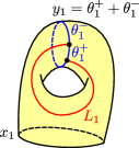
(b) The once-holed torus.

Figure 10. The two cases where $r=1$.

In the second case, the surface $\mathbf{S}$ is a once-holed torus, $\beta$ is a curve on $\mathbf{S}$, and $\Lambda$ has two components, $\beta$ and $\partial\mathbf{S}$. The length of $\beta$ is $y_{1}=\theta_{1}^{+}+\theta_{1}^{-}$, and we notice that the parameter $\theta_{1}^{+}$ can be chosen to be a twist parameter. The Weil–Petersson measure for a once-holed torus of boundary length $x_{1}$ can then be written

$$\,\mathrm{d}\mathrm{Vol}^{\mathrm{WP}}_{1,1,x_{1}}(Y)=\,\mathrm{d}y_{1}\,\mathrm{d}\theta_{1}^{+}=\,\mathrm{d}\theta_{1}^{-}\,\mathrm{d}\theta_{1}^{+}.$$

We can conclude by observing that $\cosh\left(\frac{x_{1}}{2}\right)=\cosh^{2}\left(\frac{y_{1}}{2}\right)-\sinh^{2}\left(\frac{y_{1}}{2}\right)\cosh(L_{1})$, as in the pair of pants case above, and hence

$$\sinh\left(\frac{x_{1}}{2}\right)\,\mathrm{d}x_{1}=2\sinh^{2}\left(\frac{y_{1}}{2}\right)\sinh(L_{1})\,\mathrm{d}L_{1}.$$

∎

Let us now perform the induction.

Proof of the induction of Theorem 3.11.

Let $r\geq 2$, and $\mathbf{c}$ be a generalized eight with $r$ self-intersections filling a surface $\mathbf{S}$, with a choice of opening for each intersection point. Let ${\mathbf{c}}^{\prime}$ denote the multi-loop obtained by removing the last intersection point from ${\mathbf{c}}$ the first way (as described in §2.4). Then, $\mathbf{c}^{\prime}$ is a generalized eight with $r-1$ intersections, and fills the surface $\mathbf{S}_{r-1}$. We assume that the proposition is true for the surface $\mathbf{S}_{r-1}$ and the multi-loop $\mathbf{c}^{\prime}$ (with intersections opened as they are for $\mathbf{c}$), and want to prove it for $\mathbf{S}=\mathbf{S}_{r}$ by attaching the pair of pants $\mathbf{P}_{r}$.

If $\mathbf{S}_{r}$ is a disjoint union of once-holed tori, then the property is a direct consequence of the result for $r=1$, thanks to its multiplicativity. We hence assume that it is not the case. We therefore have two cases to consider, Case (a) and Case (b).

Let $\vec{L}^{\prime}$ and $\vec{\theta}^{\prime}=(\theta_{1}^{\prime\pm},\ldots,\theta_{r-1}^{\prime\pm})$ be the parameters associated to the surface $\mathbf{S}_{r-1}$ and to ${\mathbf{c}}^{\prime}$, as constructed in §3.1. We observe that $\vec{L}^{\prime}=(L_{1},\ldots,L_{r-1})$ are the lengths of $\overline{B}_{1},\ldots,\overline{B}_{r-1}$, and in particular $\vec{L}^{\prime}$ is the same as $\vec{L}$ with the last component removed.

The parameters $(\theta_{q}^{\prime})_{q\in\{1,\ldots,r-1\}\times\{\pm\}}$, are defined as the lengths of simple portions $\overline{\mathcal{I}}_{q}^{\prime}$ contained in $\beta$ and delimited by the endpoints of the bars $\overline{B}_{1},\ldots,\overline{B}_{r-1}$. We can therefore easily relate $\vec{\theta}^{\prime}$ and $\vec{\theta}$: among the $2(r-1)$ segments $\overline{\mathcal{I}}_{q}^{\prime}$, two of them contain the endpoints of $\overline{B}_{r}$. All the other $\overline{\mathcal{I}}_{q}^{\prime}$ are also intervals $\overline{\mathcal{I}}_{q}$. As a consequence, for $k\in\{1,\ldots,r-1\}$, $\epsilon=\pm$, we have $\theta_{k}^{\epsilon}=\theta_{k}^{\prime\epsilon}$ for all except two values of $(k,\epsilon)$, namely $(n_{+},\epsilon_{+}),(n_{-},\epsilon_{-})$, for which we have the simple relations

(3.6) $$\theta_{n_{+}}^{\prime\epsilon_{+}}=\theta_{n_{+}}^{\epsilon_{+}}+\theta_{r}^{+}\qquad\text{and}\qquad\theta_{n_{-}}^{\prime\epsilon_{-}}=\theta_{n_{-}}^{\epsilon_{-}}+\theta_{r}^{-}.$$

We now proceed differently depending on the case to consider, (a) or (b).

Case (a).

In this case, $\mathbf{S}_{r}$ is obtained from $\mathbf{S}_{r-1}$ by gluing $\mathbf{P}_{r}$ to two of its boundary components. Let $\lambda_{\pm}\in\Lambda$ denote the indices of the two boundary components of $\mathbf{S}_{r-1}$ on which we glue the pair of pants $\mathbf{P}_{r}$, which satisfy $\mathrm{step}(\lambda_{\pm})<r$. By Remark 3.10, these two boundary components of $\mathbf{S}_{r-1}$ are replaced by the $n_{\mathbf{S}}$-th boundary component of $\mathbf{S}=\mathbf{S}_{r}$ when ${\mathbf{P}}_{r}$ is attached to $\mathbf{S}_{r-1}$.

Because the endpoints of the orthogeodesic $\overline{B}^{+}_{r}$ are on the multi-loop $\beta$, there exist $i_{\pm}$ such that the bar $\overline{B}_{r}^{+}$ goes from the component $\beta_{i_{-}}$ of $\beta$ to the component $\beta_{i_{+}}$ of $\beta$. It is homotopic (with endpoints gliding along $\beta$) to a succession of $5$ orthogonal segments of respective lengths $t_{r}^{-},\alpha_{r}^{-},T,\alpha_{r}^{+},t_{r}^{+}$, as shown on Figure 11. More precisely, we can lift the four geodesics $\beta_{i_{-}}$, $\Gamma_{\lambda_{-}}$, $\Gamma_{\lambda_{+}}$ and $\beta_{i_{+}}$ to the hyperbolic plane, and orient them so that they are aligned and the bar $\overline{B}^{+}_{r}$ arrives on the right of $\beta_{i_{+}}$. Then, we define:

• $H^{\pm}$ to be the orthogeodesics between $\beta_{i_{\pm}}$ and $\Gamma_{\lambda_{\pm}}$, and $H$ between $\Gamma_{\lambda_{-}}$ and $\Gamma_{\lambda_{+}}$;

• $t_{r}^{\pm}$ and $T$ to be the respective (positive) lengths of $H^{\pm}$ and $H$;

• the quantities $\alpha_{r}^{+}$ and $\alpha_{r}^{-}$ to denote the algebraic distance between the endpoints of $H^{+}$ and $H$ along $\Gamma_{\lambda_{+}}$ and between the endpoints of $H$ and $H^{-}$ along $\Gamma_{\lambda_{-}}$ respectively.

It is important in our discussion to remark that $H^{\pm}$ are contained in $\mathbf{S}_{r-1}$, so that their lengths depend only on $Y_{\mathbf{S}_{r-1}}$, the restriction of the metric $Y$ to $\mathbf{S}_{r-1}$.

Figure 11. The geometric construction in Case (a). The black dots symbolize the right-angles between the different segments.

In order to express the Weil–Petersson measure for $\mathbf{S}_{r}$, and relate it to the Weil–Petersson measure for $\mathbf{S}_{r-1}$, we need to define twist parameters along the glued components $\Gamma_{\lambda_{\pm}}$. We choose them to be the algebraic lengths $\alpha_{r}^{\pm}$. As a consequence, the expression of the Weil–Petersson measure in Fenchel–Nielsen coordinates recalled in §3.4 implies the factorization

(3.7) $$\,\mathrm{d}\mathrm{Vol}^{\mathrm{WP}}_{g_{\mathbf{S}},n_{\mathbf{S}},\mathbf{x}}(Y)=\,\mathrm{d}\alpha_{r}^{+}\,\mathrm{d}\alpha_{r}^{-}\,\mathrm{d}y_{\lambda_{+}}\,\mathrm{d}y_{\lambda_{-}}\,\mathrm{d}\mathrm{Vol}^{\mathrm{WP}}_{g_{\mathbf{S}}-1,n_{\mathbf{S}}+1,\mathbf{x}^{\prime}}(Y_{\mathbf{S}_{r-1}}),$$

where $\mathbf{x}=(x_{1},\ldots,x_{n_{\mathbf{S}}})$ and $\mathbf{x}^{\prime}=(x_{1},\ldots,x_{n_{\mathbf{S}}-1},y_{\lambda_{+}},y_{\lambda_{-}})$ correspond to the respective length-vectors of $\mathbf{S}_{r}$ and $\mathbf{S}_{r-1}$.

We can now, as in the case $r=1$, use the classic trigonometric formula for convex right-angled hexagons [5, Theorem 2.4.1 (i)], which yields

(3.8) $$\cosh(T)=\frac{\cosh\left(\frac{y_{\lambda_{+}}}{2}\right)\cosh\left(\frac{y_{\lambda_{-}}}{2}\right)+\cosh\left(\frac{x_{n_{\mathbf{S}}}}{2}\right)}{\sinh\left(\frac{y_{\lambda_{+}}}{2}\right)\sinh\left(\frac{y_{\lambda_{-}}}{2}\right)},$$

which implies that the map $x_{n_{\mathbf{S}}}\mapsto T$ is a $\mathcal{C}^{1}$-diffeomorphism onto its image, and

(3.9) $$\sinh\left(\frac{x_{n_{\mathbf{S}}}}{2}\right)\,\mathrm{d}x_{n_{\mathbf{S}}}=2\sinh\left(\frac{y_{\lambda_{+}}}{2}\right)\sinh\left(\frac{y_{\lambda_{-}}}{2}\right)\sinh(T)\,\mathrm{d}T.$$

It follows that $\prod_{j=1}^{n_{\mathbf{S}}}\sinh\left(\frac{x_{j}}{2}\right)\,\mathrm{d}\mathrm{Vol}^{\mathrm{WP}}_{g_{\mathbf{S}},n_{\mathbf{S}}}(\mathbf{x},Y)$ is equal to

$$2\sinh(T)\,\mathrm{d}T\,\mathrm{d}\alpha_{r}^{+}\,\mathrm{d}\alpha_{r}^{-}\prod_{j=1}^{n_{\mathbf{S}}-1}\sinh\left(\frac{x_{j}}{2}\right)\sinh\left(\frac{y_{\lambda_{+}}}{2}\right)\sinh\left(\frac{y_{\lambda_{-}}}{2}\right)\,\mathrm{d}\mathrm{Vol}^{\mathrm{WP}}_{g_{\mathbf{S}}-1,n_{\mathbf{S}}+1}(\mathbf{x}^{\prime},Y_{\mathbf{S}_{r-1}})$$

which, using the induction hypothesis, implies that

(3.10) $$\begin{split}&\prod_{j=1}^{n_{\mathbf{S}}}\sinh\left(\frac{x_{j}}{2}\right)\,\mathrm{d}\mathrm{Vol}^{\mathrm{WP}}_{g_{\mathbf{S}},n_{\mathbf{S}}}(\mathbf{x},Y)\\ &={2^{r}}\sinh(T)\,\mathrm{d}T\,\mathrm{d}\alpha_{r}^{+}\,\mathrm{d}\alpha_{r}^{-}\prod_{\lambda\in\Lambda^{\beta}}\sinh^{2}\left(\frac{y_{\lambda}}{2}\right)\prod_{i=1}^{r-1}\sinh(L_{i})\,\mathrm{d}L_{i}\prod_{k=1}^{r-1}\,\mathrm{d}\theta_{k}^{\prime+}\,\mathrm{d}\theta_{k}^{\prime-}\end{split}$$

where we use the observation that the length-vector $\vec{L}^{\prime}$ is equal to $(L_{1},\ldots,L_{r-1})$.

Let us now denote by $\epsilon_{r}^{+}$ and $\epsilon^{-}_{r}$ the algebraic distance from the endpoint of $H^{+}$ to the endpoint of $\overline{B}_{r}$ along $\beta_{i_{+}}$, and from the endpoint of $\overline{B}_{r}$ to the endpoint of $H^{-}$ along $\beta_{i_{-}}$ respectively, as represented in Figure 11. Let us temporarily admit the following formula (which will be checked in §3.4.5):

Lemma 3.14.

Given a fixed metric $Y_{\mathbf{S}_{r-1}}$, the map $(\alpha_{r}^{-},\alpha_{r}^{+},T)\mapsto(\epsilon_{r}^{-},\epsilon_{r}^{+},L_{r})$ is a $\mathcal{C}^{1}$-diffeomorphism onto its image, and

(3.11) $$\sinh(T)\,\mathrm{d}T\,\mathrm{d}\alpha_{r}^{-}\,\mathrm{d}\alpha_{r}^{+}=\sinh(L_{r})\,\mathrm{d}L_{r}\,\mathrm{d}\epsilon_{r}^{-}\,\mathrm{d}\epsilon_{r}^{+}.$$

We can now remark that

(3.12) $$\theta_{r}^{+}+\epsilon_{r}^{+}=\mathrm{fn}(Y_{\mathbf{S}_{r-1}})\qquad\mbox{and}\qquad\theta_{r}^{-}-\epsilon_{r}^{-}=\mathrm{fn}(Y_{\mathbf{S}_{r-1}}).$$

Indeed, for instance, the first quantity is the signed distance (measured along $\beta_{i_{+}}$) between the extremity of $H^{+}$ lying in $\beta_{i_{+}}$, and one of the bars $\overline{B}_{m_{+}}$ with $m_{+}<r$. See Figure 12.

Figure 12. The relations between the different algebraic lengths along $\beta_{i_{+}}$.

The relation (3.12) implies that in (3.11), we can change variables $(\epsilon_{r}^{-},\epsilon_{r}^{+})\rightsquigarrow(\theta_{r}^{-},\theta_{r}^{+})$ and replace $\,\mathrm{d}\epsilon_{r}^{-}\,\mathrm{d}\epsilon_{r}^{+}$ by $\,\mathrm{d}\theta_{r}^{-}\,\mathrm{d}\theta_{r}^{+}$. Our expression (3.10) then becomes

$$2^{r}\sinh(L_{r})\,\mathrm{d}L_{r}\,\mathrm{d}\theta_{r}^{-}\,\mathrm{d}\theta_{r}^{+}\prod_{\lambda\in\Lambda^{\beta}}\sinh^{2}\left(\frac{y_{\lambda}}{2}\right)\prod_{i=1}^{r-1}\sinh(L_{i})\,\mathrm{d}L_{i}\prod_{k=1}^{r-1}\,\mathrm{d}\theta_{k}^{\prime+}\,\mathrm{d}\theta_{k}^{\prime-}.$$

Now recall the relations between $\theta_{k}^{\epsilon}$ and $\theta_{k}^{\prime\epsilon}$. For $k\leq r-1$ and $\epsilon=\pm$, those parameters are equal, except from two sets of indices, for which these values differ by a translation by (3.6). Hence, our final expression for the measure is the announced one. ∎

Remark 3.15.

Part of this discussion is irrelevant when $\beta_{i_{-}}=\Gamma_{\lambda_{-}}$, because in this case, $H^{-}$ and $\alpha_{r}^{-}$ are ill-defined. The previous discussion has to be modified as follows.

• If $\beta_{i_{-}}$ is a boundary curve, then there is no twist parameter attached to it and there is no bar $\overline{B}_{k}$ arriving at $\beta_{i_{-}}$ on the other side of $\overline{B}_{r}$: we have $\theta_{r}^{-}=x_{i_{-}}=y_{i_{-}}$.

• If $\beta_{i_{-}}$ is not a boundary curve, then we can take directly $\theta_{r}^{-}$ as twist parameter, instead of the ill-defined $\alpha_{r}^{-}$.

In all cases, the final outcome of the calculation is the same, with less intermediate steps. Similar remarks can be made when $\beta_{i_{+}}=\Gamma_{\lambda_{+}}$. We skip details specific to these cases, similar and simpler than the one we treated.

Case (b).

In this case, we attach $\mathbf{P}_{r}$ to one boundary component $\Gamma_{\lambda}$ of $\mathbf{S}_{r-1}$ (with $\mathrm{step}(\lambda)<r$), and get the two new boundary components of $\mathbf{S}_{r}$ labelled $n_{\mathbf{S}}$ and $n_{\mathbf{S}}-1$.

Figure 13. The geometric construction in Case (b).

The situation is quite similar to Case (a) with a small difference, namely the fact that $\lambda_{+}=\lambda_{-}$; we therefore denote them $\lambda$. There exist $i_{\pm}$ such that the orthogeodesic $\overline{B}_{r}^{+}$ goes from $\beta_{i_{-}}$ to $\beta_{i_{+}}$. It is homotopic to a succession of $5$ orthogonal segments of respective lengths $t_{r}^{-},\alpha_{r}^{-},T,\alpha_{r}^{+},t_{r}^{+}$, as shown on Figure 13. Note that, when lifting Figure 11 and 13 in the universal cover, we obtain the same picture, the only difference being that the lifts of $\Gamma_{\lambda_{\pm}}$ now are two different lifts of the same periodic geodesic $\Gamma_{\lambda}$. We therefore define the orthogeodesics $H^{\pm}$ and $H$, as well as the lengths $t_{r}^{\pm}$, $\alpha_{r}^{\pm}$ and $T$ as in Case (a).

We choose the twist parameter to be $\alpha_{r}^{+}$. As a consequence, the expression of the Weil–Petersson measure in Fenchel–Nielsen coordinates implies the factorization

(3.13) $$\,\mathrm{d}\mathrm{Vol}^{\mathrm{WP}}_{g_{\mathbf{S}},n_{\mathbf{S}},\mathbf{x}}(Y)=\,\mathrm{d}\alpha_{r}^{+}\,\mathrm{d}y_{\lambda}\,\mathrm{d}\mathrm{Vol}^{\mathrm{WP}}_{g_{\mathbf{S}},n_{\mathbf{S}}-1,\mathbf{x}^{\prime}}(Y_{\mathbf{S}_{r-1}})$$

where $\mathbf{x}^{\prime}=(x_{1},\ldots,x_{n_{\mathbf{S}}-2},y_{\lambda})$.

We can now use the following formulas:

(3.14) $$\cosh\left(\frac{x_{n_{\mathbf{S}}}}{2}\right)=\sinh\left(\frac{\alpha}{2}\right)\sinh\left(\frac{T}{2}\right)$$

(3.15) $$\cosh\left(\frac{x_{n_{\mathbf{S}}-1}}{2}\right)=\sinh\left(\frac{y_{\lambda}-\alpha}{2}\right)\sinh\left(\frac{T}{2}\right),$$

where $\alpha$ is the distance between the two endpoints of the orthogeodesic $H$ measured along $\Gamma_{\lambda}$, as shown on Figure 14.

Figure 14. The length $\alpha$ in the pair of pants $\mathbf{P}_{r}$.

As a consequence, we make the following observation, replacing equation (3.9) in Case (a), obtained by calculating a $2\times 2$ determinant: for fixed $y_{\lambda}$, the map $(x_{n_{\mathbf{S}}-1},x_{n_{\mathbf{S}}})\mapsto(\alpha,T)$ is a $\mathcal{C}^{1}$-diffeomorphism onto its image, and

$$\sinh\left(\frac{x_{n_{\mathbf{S}}-1}}{2}\right)\sinh\left(\frac{x_{n_{\mathbf{S}}}}{2}\right)\,\mathrm{d}x_{n_{\mathbf{S}}-1}\,\mathrm{d}x_{n_{\mathbf{S}}}=2\sinh\left(\frac{y_{\lambda}}{2}\right)\sinh(T)\,\mathrm{d}\alpha\,\mathrm{d}T.$$

The rest of the proof goes along the same lines as in Case (a) and we skip details. ∎

Finally, to conclude, in all cases, the fact that the map $(\mathbf{x},Y)\in\mathcal{T}^{*}_{g_{\mathbf{S}},n_{\mathbf{S}}}\mapsto(\vec{L},\vec{\theta})$ is a $\mathcal{C}^{1}$-diffeomorphism onto its image can also obtained by induction, since at each step we checked that the maps were $\mathcal{C}^{1}$-diffeomorphisms onto their images. ∎

3.4.5. Proof of Lemma 3.14

To finish this section, there remains to prove Lemma 3.14. We also start investigating the range of definition of $\vec{L}$ and $\vec{\theta}$.

Let us consider a family of $M$ aligned geodesics $\gamma_{1},\ldots,\gamma_{M}$ on the hyperbolic plane, such that, for all $i$, $\gamma_{i+1}$ is on the left of $\gamma_{i}$ (for now, we will only take $M=3$ and $4$, but more general situations will arise in §7). For indices $i\neq j$, let $H_{ij}$ denote the orthogeodesic between $\gamma_{i}$ and $\gamma_{j}$ and $z_{ij}$ the endpoint of $H_{ij}$ lying on $\gamma_{j}$. Let us first prove one intermediate lemma in a three-geodesic configuration, illustrated in Figure 15.

Lemma 3.16.

Let $M=3$. We denote as $L$, $t$, $T$ the following orthogeodesic lengths

$$L=\ell(H_{13})\qquad t=\ell(H_{23})\qquad T=\ell(H_{12})$$

and $\epsilon$, $\alpha$ the algebraic distances

$$\epsilon=\vec{\mathrm{d}}(z_{23},z_{13})\qquad\qquad\alpha=\vec{\mathrm{d}}(z_{32},z_{12}).$$

Then, for fixed $t>0$, the map

$$\psi_{t}:\begin{cases}\mathbb{R}\times\mathbb{R}_{>0}&\rightarrow\mathbb{R}\times\mathbb{R}_{>0}\\ (\alpha,T)&\mapsto(\epsilon,L)\end{cases}$$

is a $\mathcal{C}^{1}$-diffeomorphism onto the set of real numbers $(\epsilon,L)$ such that

(3.16) $$\begin{cases}\cosh(t)\cosh(L)-\cosh(\epsilon)\sinh(t)\sinh(L)>1\\ L>t,\end{cases}$$

and its Jacobian can be expressed as

(3.17) $$\sinh(T)\,\mathrm{d}T\,\mathrm{d}\alpha=\sinh(L)\,\mathrm{d}L\,\mathrm{d}\epsilon.$$

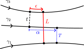
Figure 15. The three geodesics and the lengths we will study. The dots mark the points $z_{ij}$, where the geodesics meet perpendicularly.

Proof.

The fact that the image of $\{\alpha\in\mathbb{R},T>0\}$ is included in the set of $(\epsilon,L)$ satisfying the conditions (3.16) can be read from standard formulas for right-angled hexagons in hyperbolic geometry, see e.g. [5, Ch. 2 §4]:

(3.18) $$\cosh(T)=\cosh(t)\cosh(L)-\cosh(\epsilon)\sinh(t)\sinh(L)$$

(3.19) $$\cosh(L)=\cosh(t)\cosh(T)+\cosh(\alpha)\sinh(t)\sinh(T).$$

Conversely, if (3.16) holds for parameters $(L,\epsilon)$, then there exists $T\not=0$ such that (3.18) holds. This defines $T$ up to the sign, and we choose the positive solution. Another classical hyperbolic trigonometry formula states that, for this geometric situation to hold, we must have

(3.20) $$\frac{\sinh(\epsilon)}{\sinh(T)}=\frac{\sinh(\alpha)}{\sinh(L)}.$$

One can then define $\alpha$ so that the relation (3.20) holds. Note that $\alpha$ has the same sign as $\epsilon$. By using $\cosh^{2}(L)=1+\sinh^{2}(L)$ and the two relations (3.18) and (3.20), one then deduces that

$$(\cosh(L)-\cosh(t)\cosh(T))^{2}=(\cosh(\alpha)\sinh(t)\sinh(T))^{2}$$

or, in other words,

$$\cosh(L)=\cosh(t)\cosh(T)\pm\cosh(\alpha)\sinh(t)\sinh(T).$$

Because we assumed that $L>t$, we actually obtain that (3.19) holds, which means that $L$ is indeed the length of the orthogeodesic $H_{13}$ on Figure 15.

The determinant calculation (3.17) follows from (3.19) and (3.20), but it is worth writing some details. Start writing the jacobian of the change of variable as the determinant of the matrix of partial derivatives:

$$\cosh(\epsilon)\,\frac{\,\mathrm{d}L\,\mathrm{d}\epsilon}{\,\mathrm{d}T\,\mathrm{d}\alpha}=\frac{\partial L}{\partial T}\frac{\partial(\sinh(\epsilon))}{\partial\alpha}-\frac{\partial L}{\partial\alpha}\frac{\partial(\sinh(\epsilon))}{\partial T}.$$

Because of the relation (3.20), we can rewrite this as

$$\cosh(\epsilon)\,\frac{\,\mathrm{d}L\,\mathrm{d}\epsilon}{\,\mathrm{d}T\,\mathrm{d}\alpha}=\frac{\partial L}{\partial T}\frac{\cosh(\alpha)\sinh(T)}{\sinh(L)}-\frac{\partial L}{\partial\alpha}\frac{\sinh(\alpha)\cosh(T)}{\sinh(L)}.$$

An elementary calculation of $\partial L/\partial T$ and $\partial L/\partial\alpha$ from (3.19) yields that

$$\cosh(\epsilon)\,\frac{\,\mathrm{d}L\,\mathrm{d}\epsilon}{\,\mathrm{d}T\,\mathrm{d}\alpha}=\frac{\sinh(T)}{\sinh^{2}(L)}(\sinh(t)\cosh(T)+\cosh(t)\sinh(T)\cosh(\alpha)).$$

Using another classical trigonometric formula, we recognize the quantity in the bracket to be $\cosh(\epsilon)\sinh(L)$, and hence this simplifies to

$$\frac{\,\mathrm{d}L\,\mathrm{d}\epsilon}{\,\mathrm{d}T\,\mathrm{d}\alpha}=\frac{\sinh(T)}{\sinh(L)}$$

which is the desired relation. ∎

Remark 3.17.

We actually have $L\geq t+T$, so for any given $a>0$, the set $\{\alpha\in\mathbb{R},T>a\}$ is sent to a subset of the set of the set of values $(\epsilon,L)$ such that

$$\begin{cases}\cosh(t)\cosh(L)-\cosh(\epsilon)\sinh(t)\sinh(L)\geq\cosh(a)\\ L\geq t+a.\end{cases}$$

Notation 3.18.

This result provides us with a map $\phi_{t}:(\epsilon,L)\mapsto\vec{\mathrm{d}}(z_{31},z_{21})$, which corresponds to the algebraic distance along the bottom geodesic.

In order to prove Lemma 3.14, we simply apply Lemma 3.16 twice in a four-geodesic configuration, as done below. See also Figure 16.

Figure 16. The four-geodesic configuration we consider. We have represented the quantities $\tilde{T}^{+}$ and $\theta^{+}$ appearing in the statement.

Lemma 3.19.

Let $M=4$. We denote as $L$, $t^{\pm}$ and $T$ the orthogeodesic lengths

$$L=\ell(H_{14})\qquad t^{+}=\ell(H_{34})\qquad t^{-}=\ell(H_{12})\qquad T=\ell(H_{23})$$

and $\epsilon^{\pm}$, $\alpha^{\pm}$ the algebraic lengths

$$\epsilon^{+}=\vec{\mathrm{d}}(z_{34},z_{14})\qquad\alpha^{+}=\vec{\mathrm{d}}(z_{43},z_{23})\qquad\alpha^{-}=\vec{\mathrm{d}}(z_{32},z_{12})\qquad\epsilon^{-}=\vec{\mathrm{d}}(z_{41},z_{21}).$$

For fixed $t^{-},t^{+}>0$, the map

$$\begin{cases}\mathbb{R}^{2}\times\mathbb{R}_{>0}&\rightarrow\mathbb{R}^{2}\times\mathbb{R}_{>0}\\ (\alpha^{-},\alpha^{+},T)&\mapsto(\epsilon^{-},\epsilon^{+},L)\end{cases}$$

is a $\mathcal{C}^{1}$-diffeomorphism onto the set of real numbers $(\epsilon^{-},\epsilon^{+},L)$ such that

(3.21) $$\begin{cases}\cosh(t^{+})\cosh(L)-\cosh(\epsilon^{+})\sinh(t^{+})\sinh(L)>1\\ \cosh(t^{-})\cosh(\tilde{T}^{+})-\cosh(\epsilon^{-}-\theta^{+})\sinh(t^{-})\sinh(\tilde{T}^{+})>1\\ L>t^{+}\quad\text{and}\quad\tilde{T}^{+}>t^{-},\end{cases}$$

where $\tilde{T}^{+}$ is the second component of $\psi_{t^{+}}^{-1}(\epsilon^{+},L)$ and $\theta^{+}:=\phi_{t^{+}}(\epsilon^{+},L)$. Its Jacobian can be expressed as

(3.22) $$\sinh(T)\,\mathrm{d}T\,\mathrm{d}\alpha^{-}\,\mathrm{d}\alpha^{+}=\sinh(L)\,\mathrm{d}L\,\mathrm{d}\epsilon^{-}\,\mathrm{d}\epsilon^{+}.$$

Proof.

We simply apply the previous result twice, once to the three geodesics $\gamma_{1},\gamma_{3},\gamma_{4}$, and another time to $\gamma_{3},\gamma_{2},\gamma_{1}$ with reverse orientation. ∎

Remark 3.20.

We always have $L\geq t^{+}+T+t^{-}$ and $\tilde{T}^{+}\geq t^{-}+T$. Hence, for any $a>0$, the set $\{\alpha^{-},\alpha^{+}\in\mathbb{R},T>a\}$ corresponds to a subset of the set of real numbers $(\epsilon^{-},\epsilon^{+},L)$ such that

$$\begin{cases}\cosh(t^{+})\cosh(L)-\cosh(\epsilon^{+})\sinh(t^{+})\sinh(L)\geq\cosh(a)\\ \cosh(t^{-})\cosh(\tilde{T}^{+})-\cosh(\epsilon^{-}-\theta^{+})\sinh(t^{-})\sinh(\tilde{T}^{+})\geq\cosh(a)\\ L>t^{+}+a\quad\text{and}\quad\tilde{T}^{+}>t^{-}+a.\end{cases}$$

3.5. Domain of definition of the new coordinates

In this section, we discuss the range of definition $\mathfrak{D}$ of the coordinates $(\vec{L},\vec{\theta})$, which will be the domain of the integral (1.13) in the new coordinates. We prove the following statement, which describes the boundary of $\mathfrak{D}$.

Proposition 3.21.

The boundary of $\mathfrak{D}$ is contained in $\bigcup_{\lambda\in\Lambda}\{y_{\lambda}=0\}$.

Proof.

We once again proceed by induction, closely following the proof of Theorem 3.11 but making the domain of definition of the variables more explicit.

The result is trivial for $r=1$. Let us fix a metric $Y_{\mathbf{S}_{r-1}}\in\mathcal{T}_{g_{\mathbf{S}_{r-1}},n_{\mathbf{S}_{r-1}}}^{*}$ and describe the domain of definition of the three new coordinates $(\theta_{r}^{-},\theta_{r}^{+},L_{r})$ defined when attaching the pair of pants ${\mathbf{P}}_{r}$. We note that there exists a unique hyperbolic metric associated to any set of Fenchel–Nielsen coordinates. Hence, the constraints on the new variables are:

• $(\epsilon_{r}^{+},\epsilon_{r}^{-},L_{r})$ need to belong to the image of the diffeomorphism in Lemma 3.19 – we call this the local constraint;

• the new boundary components of the pair of pants need to be of positive length, i.e. $x_{n_{\mathbf{S}}}>0$ in Case (a) and $x_{n_{\mathbf{S}}},x_{n_{\mathbf{S}}-1}>0$ in Case (b) – we call this the global constraint.

We prove Proposition 3.21 by proving that the global constraints are stronger than the local constraints. Indeed, in Case (a), because of (3.8), the global constraint is equivalent to

$$\cosh(T)>\frac{\cosh\left(\frac{y_{\lambda_{+}}}{2}\right)\cosh\left(\frac{y_{\lambda_{-}}}{2}\right)+1}{\sinh\left(\frac{y_{\lambda_{+}}}{2}\right)\sinh\left(\frac{y_{\lambda_{-}}}{2}\right)}.$$

Note that the quantity

$$a:=\operatorname{argcosh}\Big{(}\frac{\cosh\left(\frac{y_{\lambda_{+}}}{2}\right)\cosh\left(\frac{y_{\lambda_{-}}}{2}\right)+1}{\sinh\left(\frac{y_{\lambda_{+}}}{2}\right)\sinh\left(\frac{y_{\lambda_{-}}}{2}\right)}\Big{)}>0,$$

only depends $y_{\lambda_{+}}$ and $y_{\lambda_{-}}$, i.e. on the metric $Y_{\mathbf{S}_{r-1}}$ in $\mathcal{T}_{g_{\mathbf{S}}-1,n_{\mathbf{S}}+1}^{*}$ that we are considering to be fixed. Hence, the global constraint implies the $T>a$, where $a$ is fixed. By Remark 3.20, this implies strictly stronger conditions than the original local constraints, which is what we wanted to check.

In Case (b), the formulas (3.14) and (3.15) are equivalent to

$$\cosh(T)=\frac{\cosh^{2}\left(\frac{\alpha}{2}\right)+\cosh(x_{n_{\mathbf{S}}})}{\sinh^{2}\left(\frac{\alpha}{2}\right)}\quad\mbox{and}\quad\cosh({{T}})=\frac{\cosh^{2}\left(\frac{y_{\lambda}-\alpha}{2}\right)+\cosh(x_{n_{\mathbf{S}}-1})}{\sinh^{2}\left(\frac{y_{\lambda}-\alpha}{2}\right)}.$$

Thus the new global constraints are equivalent to

$$\cosh({{T}})>\frac{\cosh^{2}\left(\frac{\alpha}{2}\right)+1}{\sinh^{2}\left(\frac{\alpha}{2}\right)}=1+\frac{2}{\sinh^{2}\left(\frac{\alpha}{2}\right)}\quad\mbox{and}\quad\cosh({{T}})>1+\frac{2}{\sinh^{2}\left(\frac{y_{\lambda}-\alpha}{2}\right)}.$$

Define $a:=\operatorname{argcosh}(1+2/\sinh^{2}\left(\frac{y_{\lambda}}{2}\right))$. Since $0<\alpha<y_{\lambda}$, the two global constraints imply that $T>a>0$, which allows to conclude as in Case (a). ∎

3.6. A priori bounds on Fenchel–Nielsen parameters

We shall need some rough a priori bounds on the parameters $y_{\lambda}=\ell_{Y}(\Gamma_{\lambda})$ for $\lambda\in\Lambda$ and $\theta_{q}$ for $q\in\Theta$, that grow at most linearly with respect to $\ell_{Y}({\mathbf{c}})$.

Proposition 3.22.

On the level set $\{Y\in\mathcal{T}_{g_{\mathbf{S}},n_{\mathbf{S}}}^{*}\,:\,\ell_{Y}({\mathbf{c}})=\ell\}$, we have

(3.23) $$\forall\lambda\in\Lambda, \quad 0\leq y_{\lambda}\leq\ell$$

(3.24) $$\forall q\in\Theta, \quad|\theta_{q}|\leq 2\ell$$

and the twist parameters $(\alpha_{\lambda})_{\lambda\in\Lambda_{\mathrm{in}}}$ constructed in the proof of Theorem 3.11 satisfy

(3.25) $$\forall\lambda\in\Lambda_{\mathrm{in}},\quad|\alpha_{\lambda}|\leq 3\ell.$$

The proof relies on elementary hyperbolic trigonometry, and in particular the following lemma.

Lemma 3.23.

Let $Y$ be a compact hyperbolic surface with two simple, closed geodesics $\gamma_{1},\gamma_{2}$. We assume that $\gamma_{1}$ and $\gamma_{2}$ are either disjoint or equal. Let $H$ be a simple orthogeodesic segment going from $\gamma_{1}$ to $\gamma_{2}$, not intersecting $\gamma_{1}$ and $\gamma_{2}$ in its interior. Then, $\sinh(\ell(\gamma_{1})/2)\sinh(\ell(H))\geq 1$.

Proof.

If $\gamma_{1}=\gamma_{2}$, this is a direct consequence of the collar lemma [5, Theorem 4.1.1]. If the two geodesics are disjoint, then the surface filled by $\gamma_{1}$, $\gamma_{2}$ and $H$ is a pair of pants. Cutting this pair of pants along its orthogeodesics, we obtain a convex right-angled hexagon with consecutive sides of length $\ell(\gamma_{1})/2$, $\ell(H)$ and $\ell(\gamma_{2})/2$. We can further cut this hexagon and obtain a right-angled pentagon with consecutive side-lengths $\ell(\gamma_{1})/2$ and $\ell(H)$, which implies the claim by [5, Lemma 2.3.5]. ∎

We use this lemma to prove the following.

Lemma 3.24.

Let $Y$ be a compact hyperbolic surface with:

• three simple oriented closed geodesics $\gamma_{1},\gamma_{2},\gamma_{3}$;

• an orthogeodesic $H_{12}$ leaving from the right of $\gamma_{1}$ and arriving at the left of $\gamma_{2}$;

• an orthogeodesic $H_{23}$ leaving from the right of $\gamma_{2}$ and arriving at the left of $\gamma_{3}$.

Let $J\subset\gamma_{2}$ be the segment joining $t(H_{12})$ to $o(H_{23})$ and $H$ be the orthogeodesic from $\gamma_{1}$ to $\gamma_{3}$, homotopic with gliding endpoints to $H_{12}\mathord{\mathchoice{\,\vbox{\hbox{\scalebox{0.5}{$\displaystyle\bullet$}}}\,}{\,\vbox{\hbox{\scalebox{0.5}{$\textstyle\bullet$}}}\,}{\,\vbox{\hbox{\scalebox{0.5}{$\scriptstyle\bullet$}}}\,}{\,\vbox{\hbox{\scalebox{0.5}{$\scriptscriptstyle\bullet$}}}\,}}J\mathord{\mathchoice{\,\vbox{\hbox{\scalebox{0.5}{$\displaystyle\bullet$}}}\,}{\,\vbox{\hbox{\scalebox{0.5}{$\textstyle\bullet$}}}\,}{\,\vbox{\hbox{\scalebox{0.5}{$\scriptstyle\bullet$}}}\,}{\,\vbox{\hbox{\scalebox{0.5}{$\scriptscriptstyle\bullet$}}}\,}}H_{23}$. Then, if $\gamma$ denotes the geodesic representative of the homotopy class $\gamma_{1}\mathord{\mathchoice{\,\vbox{\hbox{\scalebox{0.5}{$\displaystyle\bullet$}}}\,}{\,\vbox{\hbox{\scalebox{0.5}{$\textstyle\bullet$}}}\,}{\,\vbox{\hbox{\scalebox{0.5}{$\scriptstyle\bullet$}}}\,}{\,\vbox{\hbox{\scalebox{0.5}{$\scriptscriptstyle\bullet$}}}\,}}H\mathord{\mathchoice{\,\vbox{\hbox{\scalebox{0.5}{$\displaystyle\bullet$}}}\,}{\,\vbox{\hbox{\scalebox{0.5}{$\textstyle\bullet$}}}\,}{\,\vbox{\hbox{\scalebox{0.5}{$\scriptstyle\bullet$}}}\,}{\,\vbox{\hbox{\scalebox{0.5}{$\scriptscriptstyle\bullet$}}}\,}}\gamma_{3}\mathord{\mathchoice{\,\vbox{\hbox{\scalebox{0.5}{$\displaystyle\bullet$}}}\,}{\,\vbox{\hbox{\scalebox{0.5}{$\textstyle\bullet$}}}\,}{\,\vbox{\hbox{\scalebox{0.5}{$\scriptstyle\bullet$}}}\,}{\,\vbox{\hbox{\scalebox{0.5}{$\scriptscriptstyle\bullet$}}}\,}}H^{-1}$, we have

(3.26) $$\cosh\left(\frac{\ell(\gamma)}{2}\right)\geq\cosh(\ell(J)).$$

Of course, the orientations of $\gamma_{1}$, $\gamma_{2}$ and $\gamma_{3}$ are irrelevant in the length estimate, but serve to describe the isotopy class of the picture $\gamma_{1}\cup\gamma_{2}\cup\gamma_{2}\cup H_{12}\cup H_{23}$.

Proof.

The geodesic $\gamma$ is a figure eight, going around the two closed geodesics $\gamma_{1}$ and $\gamma_{3}$, connected by the orthogeodesic $H$. It then follows that

$$\cosh\left(\frac{\ell(\gamma)}{2}\right) =\cosh\left(\frac{\ell(\gamma_{1})}{2}\right)\cosh\left(\frac{\ell(\gamma_{3})}{2}\right)+\cosh(H)\sinh\left(\frac{\ell(\gamma_{1})}{2}\right)\sinh\left(\frac{\ell(\gamma_{3})}{2}\right)$$

$$\geq\cosh(H)\sinh\left(\frac{\ell(\gamma_{1})}{2}\right)\sinh\left(\frac{\ell(\gamma_{3})}{2}\right).$$

Expressing the length of $H$ in terms of the lengths of $J$ and $H_{12}$, $H_{23}$, we obtain

$$\cosh(H) =\cosh(\ell(H_{12}))\cosh(\ell(H_{23}))+\cosh(\ell(J))\sinh(\ell(H_{12}))\sinh(\ell(H_{23}))$$

$$\geq\cosh(\ell(J))\sinh(\ell(H_{12}))\sinh(\ell(H_{23})).$$

By Lemma 3.23, $\sinh(\ell(\gamma_{1})/2)\sinh(\ell(H_{12}))\geq 1$ and $\sinh(\ell(\gamma_{3})/2)\sinh(\ell(H_{23}))\geq 1$, which leads to our claim. ∎

We are now ready to proceed to the proofs of the bounds.

Proof of Proposition 3.22.

The upper bound on $y_{\lambda}$ is a direct consequence of Remark 3.7, which states that $\Gamma_{\lambda}$ is freely homotopic to a path $\Gamma_{\lambda,\mathrm{init}}$ on $\mathbf{c}$, and hence

$$y_{\lambda}=\ell_{Y}(\Gamma_{\lambda})\leq\ell(\Gamma_{\lambda,\mathrm{init}})\leq\ell({\mathbf{c}})=\ell.$$

Let us now prove the bound on $\theta_{q}$ for an index $q\in\Theta$.

• If $q$ is a U-turn parameter, then we simply observe that $0\leq\theta_{q}\leq\ell(\beta_{\lambda(q)})\leq\ell$.

• If $q$ is a crossing parameter, we apply Lemma 3.24 to the simple closed geodesics $\gamma_{1}=\beta_{\lambda(\sigma^{-1}q)}$, $\gamma_{2}=\beta_{\lambda(q)}$ and $\gamma_{3}=\beta_{\lambda(\sigma q)}$, with the orthogeodesics $H_{12}=\overline{B}_{q}$ and $H_{23}=\overline{B}_{\sigma q}$, so that $J=\overline{\mathcal{I}}_{q}$. We check that the figure-eight $\gamma$ produced by the lemma is freely homotopic to a loop $\gamma_{\mathrm{init}}$ drawn on $\mathbf{c}$, going along $\beta_{\lambda(\sigma^{-1}q),\mathrm{init}}$, $\beta_{\lambda(\sigma q),\mathrm{init}}$ and twice $\mathcal{I}_{q,\mathrm{init}}$. We conclude that

  $$\cosh(\theta_{q})\leq\cosh(\ell(\gamma))\leq\cosh(2\ell).$$

The bounds on the twist parameters are obtained the same way, constructing for each case (Case (a) and (b)) a figure-eight $\gamma$ such that $|\alpha_{\lambda}|\leq\ell(\gamma)\leq 3\ell$ (the factor of $3$ being there for Case (b), due to repeated portions of $\mathbf{c}$ used to describe the homotopy class of $\gamma$). ∎

3.7. Polynomial bounds on volumes and the case of double-filling loops

One can straightforwardly deduce from the apriori bound on Fenchel–Nielsen parameters, Proposition 3.22, a rough polynomial upper bound on the volume of the set of hyperbolic surfaces $Y\in\mathcal{T}^{*}_{g_{\mathbf{S}},n_{\mathbf{S}}}$ such that $\ell_{Y}({\mathbf{c}})\leq\ell$. A similar statement was obtained when $\mathbf{S}$ is a once-holed torus in [2, eq. (8.4)].

Corollary 3.25.

For any family of distinct indices $(i_{j},i_{j}^{\prime})_{1\leq j\leq k}$ in $\partial\mathbf{S}$, any $\ell\geq 0$,

(3.27) $$\int_{\ell_{Y}({\mathbf{c}})\leq\ell}\prod_{j=1}^{k}\delta(x_{i_{j}}-x_{i_{j}^{\prime}})\,\mathrm{d}\mathrm{Vol}^{\mathrm{WP}}_{g_{\mathbf{S}},n_{\mathbf{S}}}(\mathbf{x},Y)\leq(3\ell)^{3\chi(\mathbf{S})}.$$

Proof.

We simply write the expression of $\,\mathrm{d}\mathrm{Vol}^{\mathrm{WP}}_{g_{\mathbf{S}},n_{\mathbf{S}}}(\mathbf{x},Y)$ in Fenchel–Nielsen coordinates as in (3.1), and use the bounds given by Proposition 3.22 on the lengths and twist angles. ∎

Remark 3.26.

We have assumed at the beginning of §3 that the loop $\mathbf{c}$ is a generalized eight, and therefore, as of now, we have only proven Corollary 3.25 for generalized eights. For the sake of the following application, it will be useful to observe that this result can be extended to any multi-loop $\mathbf{c}$. This proof relies on definitions from Section 11 and can be omitted at first read; it is only presented here for completeness and to allow to state the interesting Lemma 3.27 below.

Proof of Corollary 3.25 for general loops.

Let $\mathbf{c}^{\prime}$ be a skeleton of $\mathbf{c}$, and $\mathbf{S}^{\prime}$ be the surface filled by $\mathbf{c}^{\prime}$. If $\mathbf{S}^{\prime}=\mathbf{S}$, then by Proposition 11.13, $\ell_{Y}({\mathbf{c}}^{\prime})\leq\ell_{Y}({\mathbf{c}})$, from which we deduce the claim. Otherwise, $\mathbf{S}$ is obtained from $\mathbf{S}^{\prime}$ by gluing a finite number of cylinders and adding cylindrical bars. We add the corresponding twist parameters to our coordinate system and remove the $\theta_{q}$ that have become redundant. Corollary 3.25 persists because we can choose those twist parameters so that they still satisfy (3.25), by the same proof. ∎

As in [2, §8.1], we can use polynomial volume bounds to prove the following special case of our main result, Theorem 1.23, for double-filling loops (defined in Definition 1.21).

Lemma 3.27.

If $\mathbf{c}$ is double-filling, then $\mathcal{J}\in\mathcal{R}_{w}^{\mathrm{N}}$ and

$$\lVert\mathcal{J}\rVert_{\mathcal{R}_{w}^{\mathrm{N}}}\leq\mathrm{fn}(g_{\mathbf{S}},n_{\mathbf{S}},\mathrm{K},\mathrm{N})\prod_{j\in V}\|\tilde{g}_{j}\|_{\mathcal{F}^{\mathrm{K}_{j},\mathrm{N}_{j}}}.$$

Proof of Lemma 3.27.

Let us write

$$\int_{0}^{\ell}|\mathcal{J}(s)|\,\mathrm{d}s\leq\int_{\ell_{Y}({\mathbf{c}})\leq\ell}\,\prod_{j\in V}|f_{j}(x_{j})|\prod_{j=1}^{k}x_{i_{j}}\delta(x_{i_{j}}-x_{i_{j}^{\prime}})\,\mathrm{d}\mathrm{Vol}^{\mathrm{WP}}_{g_{\mathbf{S}},n_{\mathbf{S}}}(\mathbf{x},Y).$$

By hypothesis on the functions $f_{j}$ and using equation (1.8) on $\tilde{g}_{j}$, we have for each $j\in V$,

$$|f_{j}(x_{j})|\leq\mathrm{fn}(\mathrm{K},\mathrm{N})\|\tilde{g}_{j}\|_{\mathcal{F}^{\mathrm{K}_{j},\mathrm{N}_{j}}}(1+x_{j})^{\mathrm{K}_{j}-1}e^{x_{j}/2}$$

and for each $1\leq j\leq k$, $x_{i_{j}}\leq e^{x_{i_{j}}/2}$. By Proposition 1.30, if $\ell_{Y}({\mathbf{c}})\leq\ell$ and $\mathbf{c}$ is double-filling, then $\sum_{j=1}^{n_{\mathbf{S}}}x_{j}\leq\ell$ and hence

$$\prod_{j\in V}|f_{j}(x_{j})|\prod_{j=1}^{k}x_{i_{j}}\leq\mathrm{fn}(\mathrm{K},\mathrm{N})\prod_{j\in V}\|\tilde{g}_{j}\|_{\mathcal{F}^{\mathrm{K}_{j},\mathrm{N}_{j}}}(1+\ell)^{\sum_{j\in V}(\mathrm{K}_{j}-1)}e^{\ell/2}.$$

With Corollary 3.25, using the hypothesis $\mathrm{K}_{j}\leq\mathrm{N}_{j}$ and the definition $\mathrm{N}=\sum_{j\in V}\mathrm{N}_{j}+3\chi(\mathbf{S})+1$, this implies that

$$\int_{0}^{\ell}|\mathcal{J}(s)|\,\mathrm{d}s\leq\mathrm{fn}(g_{\mathbf{S}},n_{\mathbf{S}},\mathrm{K},\mathrm{N})\prod_{j\in V}\|\tilde{g}_{j}\|_{\mathcal{F}^{\mathrm{K}_{j},\mathrm{N}_{j}}}(1+\ell)^{\mathrm{N}-1}e^{\ell/2},$$

which allows us to conclude and to obtain the claimed bound. ∎

Remark 3.28.

Had we not assumed that $\mathbf{c}$ was double-filling, Proposition 1.30 would only have implied that

(3.28) $$\int_{0}^{\ell}|\mathcal{J}(s)|\,\mathrm{d}s\leq\mathrm{fn}(g_{\mathbf{S}},n_{\mathbf{S}},\mathrm{K},\mathrm{N})\prod_{j\in V}\|\tilde{g}_{j}\|_{\mathcal{F}^{\mathrm{K}_{j},\mathrm{N}_{j}}}(1+\ell)^{\mathrm{N}-1}e^{\ell},$$

i.e. a similar upper bound but without the factor $1/2$ in the exponential, which is not enough to conclude to Theorem 1.23.

4. Expression of length functions in the new coordinate system

The aim of this section is to give explicit expressions in the coordinates $(\vec{L},\vec{\theta})$ for the length $\ell_{Y}({\mathbf{c}})$, but also for all the lengths $y_{\lambda}$ of the multi-curve $(\Gamma_{\lambda})_{\lambda\in\Lambda}$ defined in §3.2.

4.1. Trajectories in $T^{1}{\mathbf{S}}$ and multiplication in $\mathrm{SL}(2,\mathbb{R})$

It is a classical fact that $\mathcal{T}^{*}_{g_{\mathbf{S}},n_{\mathbf{S}}}$ may be seen as the space of discrete faithful representations of the fundamental group $\pi_{1}(\mathbf{S})$ into $\mathrm{PSL}(2,\mathbb{R})$ (modulo conjugacy). Moreover, if $Y\in\mathcal{T}^{*}_{g_{\mathbf{S}},n_{\mathbf{S}}}$ corresponds to the representation $\rho:\pi_{1}(\mathbf{S})\longrightarrow\mathrm{PSL}(2,\mathbb{R})$, we can express all lengths thanks to the trace of $\rho$:

(4.1) $$2\cosh\left(\frac{\ell_{Y}(\gamma)}{2}\right)=|{\rm Tr}\,\rho(\gamma)|$$

(where $\rho(\gamma)\in\mathrm{PSL}(2,\mathbb{R})$ is the image under $\rho$ of the homotopy class of $\gamma$). Our method to express lengths in the new coordinates consists in providing an explicit expression for $\rho(\gamma)$ in (4.1), by writing a representative of the homotopy class of $\gamma$ as a succession of orthogonal segments.

We recall that the unit tangent bundle $T^{1}\mathbb{H}^{2}$ itself can be identified with $\mathrm{PSL}(2,\mathbb{R})$. We can then identify different geometric actions on $T^{1}\mathbb{H}^{2}$ with the right-multiplication by a specific matrix: $a^{t}$ is the action of the geodesic flow at time $t$, $w^{t}$ the conjugate of the geodesic flow by a rotation of angle $\pi/2$, and $k^{\theta}$ the rotation of angle $\theta$ by $k^{\theta}$, where

(4.2) $$a^{t}=\begin{pmatrix}e^{\frac{t}{2}}&0\\ 0&e^{-\frac{t}{2}}\end{pmatrix}\qquad w^{t}=\begin{pmatrix}\cosh\left(\frac{t}{2}\right)&\sinh\left(\frac{t}{2}\right)\\ \sinh\left(\frac{t}{2}\right)&\cosh\left(\frac{t}{2}\right)\end{pmatrix}\qquad k^{\theta}=\begin{pmatrix}\cos\left(\frac{\theta}{2}\right)&\sin\left(\frac{\theta}{2}\right)\\ -\sin\left(\frac{\theta}{2}\right)&\cos\left(\frac{\theta}{2}\right)\end{pmatrix}.$$

These moves are represented on Figure 17.

Figure 17. The moves corresponding to the matrices $a^{t}$, $w^{t}$ and $k^{\theta}$.

It is important to note that, while $a^{t}$ always has non-negative entries, this is true of $w^{t}$ only if $t\geq 0$. In what follows, a lot of effort is devoted to using $w^{t}$ only for $t\geq 0$.

4.2. Expression of $\ell_{Y}({\mathbf{c}})$ in the new coordinates

Let us now focus on finding an expression for $\ell_{Y}(\mathbf{c})$ in terms of $(\vec{L},\vec{\theta})$. We shall do so component by component, i.e. provide an expression for the $i$th component $\mathbf{c}_{i}$ of $\mathbf{c}$ for $i\in\{1,\ldots,\mathfrak{n}\}$. Oftenwise, we will focus on one component $\mathbf{c}_{i}$ at a time, in which case we will drop the mention of $i$ to lighten notations. This shall always be mentioned, to avoid any confusion.

4.2.1. Piecewise geodesic representative of ${\mathbf{c}_{i}}$

First, we recall that we saw in (2.7) that the homotopy class of ${\mathbf{c}}^{\mathrm{op}}_{i}$ can be written, for any index $q\in\Theta^{i}$, as

$${\mathbf{c}}^{\mathrm{op}}_{i}=p(q)\mathord{\mathchoice{\,\vbox{\hbox{\scalebox{0.5}{$\displaystyle\bullet$}}}\,}{\,\vbox{\hbox{\scalebox{0.5}{$\textstyle\bullet$}}}\,}{\,\vbox{\hbox{\scalebox{0.5}{$\scriptstyle\bullet$}}}\,}{\,\vbox{\hbox{\scalebox{0.5}{$\scriptscriptstyle\bullet$}}}\,}}p(\sigma q)\mathord{\mathchoice{\,\vbox{\hbox{\scalebox{0.5}{$\displaystyle\bullet$}}}\,}{\,\vbox{\hbox{\scalebox{0.5}{$\textstyle\bullet$}}}\,}{\,\vbox{\hbox{\scalebox{0.5}{$\scriptstyle\bullet$}}}\,}{\,\vbox{\hbox{\scalebox{0.5}{$\scriptscriptstyle\bullet$}}}\,}}\ldots\mathord{\mathchoice{\,\vbox{\hbox{\scalebox{0.5}{$\displaystyle\bullet$}}}\,}{\,\vbox{\hbox{\scalebox{0.5}{$\textstyle\bullet$}}}\,}{\,\vbox{\hbox{\scalebox{0.5}{$\scriptstyle\bullet$}}}\,}{\,\vbox{\hbox{\scalebox{0.5}{$\scriptscriptstyle\bullet$}}}\,}}p(\sigma^{n_{i}-1}q)$$

where, for any $q^{\prime}$, $p(q^{\prime})$ is the concatenation of the bar $B_{q^{\prime}}$ and the simple portion $\mathcal{I}_{q^{\prime}}$.

Consider a point $Y\in\mathcal{T}^{*}_{g_{\mathbf{S}},n_{\mathbf{S}}}$. As suggested in Remark 2.8, we can pick our representative so that $\beta$ is a multi-geodesic. We then consider the representative of the homotopy class of ${\mathbf{c}}_{i}$ given by a cyclic succession of orthogonal geodesics segments:

(4.3) $$\bar{p}(q)\mathord{\mathchoice{\,\vbox{\hbox{\scalebox{0.5}{$\displaystyle\bullet$}}}\,}{\,\vbox{\hbox{\scalebox{0.5}{$\textstyle\bullet$}}}\,}{\,\vbox{\hbox{\scalebox{0.5}{$\scriptstyle\bullet$}}}\,}{\,\vbox{\hbox{\scalebox{0.5}{$\scriptscriptstyle\bullet$}}}\,}}\bar{p}(\sigma(q))\mathord{\mathchoice{\,\vbox{\hbox{\scalebox{0.5}{$\displaystyle\bullet$}}}\,}{\,\vbox{\hbox{\scalebox{0.5}{$\textstyle\bullet$}}}\,}{\,\vbox{\hbox{\scalebox{0.5}{$\scriptstyle\bullet$}}}\,}{\,\vbox{\hbox{\scalebox{0.5}{$\scriptscriptstyle\bullet$}}}\,}}\ldots\mathord{\mathchoice{\,\vbox{\hbox{\scalebox{0.5}{$\displaystyle\bullet$}}}\,}{\,\vbox{\hbox{\scalebox{0.5}{$\textstyle\bullet$}}}\,}{\,\vbox{\hbox{\scalebox{0.5}{$\scriptstyle\bullet$}}}\,}{\,\vbox{\hbox{\scalebox{0.5}{$\scriptscriptstyle\bullet$}}}\,}}\bar{p}(\sigma^{n_{i}-1}q)$$

for a $q\in\Theta^{i}$, where $\bar{p}(q):=\overline{B}_{q}\mathord{\mathchoice{\,\vbox{\hbox{\scalebox{0.5}{$\displaystyle\bullet$}}}\,}{\,\vbox{\hbox{\scalebox{0.5}{$\textstyle\bullet$}}}\,}{\,\vbox{\hbox{\scalebox{0.5}{$\scriptstyle\bullet$}}}\,}{\,\vbox{\hbox{\scalebox{0.5}{$\scriptscriptstyle\bullet$}}}\,}}\overline{\mathcal{I}}_{q}.$ Each bar $\overline{B}_{q}$ is now an orthogeodesic from $\beta_{\lambda(\sigma^{-1}q)}$ to $\beta_{\lambda(q)}$.

For the rest of §4.2, it will be convenient to use the relabelling of $\Theta$ introduced in §2.5.2, which allows us to identify $\Theta^{i}$ with the cyclic set $\mathbb{Z}_{n_{i}}=\mathbb{Z}\diagup n_{i}\mathbb{Z}$. Through this identification, going through the elements $k\in\mathbb{Z}_{n_{i}}$ corresponds to going through the elements $\sigma^{k}q$ in (4.3). We will therefore write $\overline{B}(i,k)=\overline{B}(\sigma^{k}q)$, $\overline{\mathcal{I}}(i,k)=\overline{\mathcal{I}}(\sigma^{k}q)$, $\theta(i,k)=\theta(\sigma^{k}q)$ etc. Following Notation 3.3, we will also write $L(i,k)=L(\sigma^{k}q)$ and $\epsilon L(i,k)=\epsilon L(\sigma^{k}q)$. As a consequence, the consecutive lengths of all the segments encountered in (4.3) are (up to cyclic permutation)

$$L(i,1),\theta(i,1),\ldots,L(i,n_{i}),\theta(i,n_{i}).$$

The sign of $\epsilon L(i,k)$ tells us in which direction the bar $\overline{B}(i,k)$ is taken at the step $k$.

4.2.2. Lift of ${\mathbf{c}}$ to the universal cover

We now consider a lift of the closed path (4.3) to the universal cover of $\mathbf{S}$, identified with a subset of the hyperbolic plane. For each index $q\in{\mathbf{\Theta}}^{i}$, let $\tilde{\beta}_{q}\subset\mathbb{H}^{2}$ be a lift of the geodesic $\beta_{\lambda(q)}$ such that, if $\tilde{B}_{\sigma^{-1}q,q}$ denotes the oriented orthogeodesic going from $\tilde{\beta}_{\sigma^{-1}q}$ to $\tilde{\beta}_{q}$, then $\tilde{B}_{\sigma^{-1}q,q}$ projects down to $\overline{B}_{q}$ on the surface.

Whilst there was a priori no natural orientation for the multi-curve $\beta$ on $\mathbf{S}$, we can now orient the lifts $\tilde{\beta}_{q}$ so that the bar $\tilde{B}_{\sigma^{-1}q,q}$ arrives on the right of $\tilde{\beta}_{q}$ for each $q\in\mathbf{\Theta}^{i}$ with $\operatorname{Sign}(q)=+$ and on the left otherwise. We then make the following crucial observation.

Lemma 4.1.

The geodesics $(\tilde{\beta}_{q})_{q\in\mathbf{\Theta}^{i}}$ are disjoint and, for any $q\in\mathbf{\Theta}^{i}$, $\tilde{\beta}_{q}$ and $\tilde{\beta}_{\sigma q}$ are aligned. $\tilde{\beta}_{\sigma q}$ is on the left of $\tilde{\beta}_{q}$ if and only if $\operatorname{Sign}(q)=+$.

We denote by $\tilde{\mathcal{I}}_{q}\subset\tilde{\beta}_{q}$ the segment between the endpoint of $\tilde{B}_{\sigma^{-1}q,q}$ and the origin of $\tilde{B}_{q,\sigma q}$. Then the segment $\tilde{\mathcal{I}}_{q}$ projects down to the segment $\overline{\mathcal{I}}_{q}$ on the surface. If we call $\tilde{p}(q)=\tilde{B}_{\sigma^{-1}q,q}\mathord{\mathchoice{\,\vbox{\hbox{\scalebox{0.5}{$\displaystyle\bullet$}}}\,}{\,\vbox{\hbox{\scalebox{0.5}{$\textstyle\bullet$}}}\,}{\,\vbox{\hbox{\scalebox{0.5}{$\scriptstyle\bullet$}}}\,}{\,\vbox{\hbox{\scalebox{0.5}{$\scriptscriptstyle\bullet$}}}\,}}\tilde{\mathcal{I}}(q)$, then the infinite concatenation $\mathord{\mathchoice{\,\vbox{\hbox{\scalebox{0.5}{$\displaystyle\bullet$}}}\,}{\,\vbox{\hbox{\scalebox{0.5}{$\textstyle\bullet$}}}\,}{\,\vbox{\hbox{\scalebox{0.5}{$\scriptstyle\bullet$}}}\,}{\,\vbox{\hbox{\scalebox{0.5}{$\scriptscriptstyle\bullet$}}}\,}}_{q\in{\mathbf{\Theta}}^{i}}\;\tilde{p}(q)$ of orthogonal geodesics segments in the hyperbolic plane projects down to (4.3) on the surface. We shall denote by $\tilde{\mathbf{c}}_{i}$ the infinite geodesic homotopic to $\mathord{\mathchoice{\,\vbox{\hbox{\scalebox{0.5}{$\displaystyle\bullet$}}}\,}{\,\vbox{\hbox{\scalebox{0.5}{$\textstyle\bullet$}}}\,}{\,\vbox{\hbox{\scalebox{0.5}{$\scriptstyle\bullet$}}}\,}{\,\vbox{\hbox{\scalebox{0.5}{$\scriptscriptstyle\bullet$}}}\,}}_{q\in{\mathbf{\Theta}}^{i}}\;\tilde{p}(q)$ in the hyperbolic plane.

Notation 4.2.

The notation $\tilde{B}_{mn}$, for the moment only defined for $n=\sigma m$, may be extended to arbitrary $m,n\in{\mathbf{\Theta}}^{i}$. We call $\tilde{B}_{mn}\subset\mathbb{H}^{2}$ the oriented orthogeodesic segment from $\tilde{\beta}_{m}$ to $\tilde{\beta}_{n}$. We denote by $L_{mn}>0$ its length and $z_{mn}\in\tilde{\beta}_{n}$ its terminus.

4.2.3. Expression of the length of $\mathbf{c}_{i}$ as a trace

Starting from (4.3) we now find a formula expressing each $\ell_{Y}({\mathbf{c}}_{i})$ as the trace of a product of matrices.

Lemma 4.3.

For $i\in\{1,\ldots,\mathfrak{n}\}$, the length of the component ${\mathbf{c}}_{i}$ is given by the formula

(4.4) $$\cosh\left(\frac{\ell_{Y}({\mathbf{c}}_{i})}{2}\right)=\frac{1}{2}\,{\rm Tr}\left(a_{1}^{i}b_{1}^{i}\ldots a_{n_{i}}^{i}b_{n_{i}}^{i}\right)$$

where the matrices $a_{k}^{i},b_{k}^{i}$ are defined by

(4.5) $$a_{k}^{i}=a^{\epsilon L(i,k)}=\begin{pmatrix}e^{\frac{\epsilon L(i,k)}{2}}&0\\ 0&e^{-\frac{\epsilon L(i,k)}{2}}\end{pmatrix}\qquad b_{k}^{i}=w^{\theta(i,k)}=\begin{pmatrix}\cosh\left(\frac{\theta(i,k)}{2}\right)&\sinh\left(\frac{\theta(i,k)}{2}\right)\\ \sinh\left(\frac{\theta(i,k)}{2}\right)&\cosh\left(\frac{\theta(i,k)}{2}\right)\end{pmatrix}.$$

Proof.

For the proof, let us fix a value of $i$. As explained at the beginning of this section, the elements of $\Theta^{i}$ are labelled $(i,k)$ with $k\in\mathbb{Z}_{n_{i}}$. To lighten notations, we shall omit the mention of $i$, for instance writing $n_{i}=n$, $L_{k}=L(i,k)$, $\theta(i,k)=\theta_{k}$, etc.

Let $v$ denote the unit vector tangent to the bar $\overline{B}_{1}=\overline{B}(i,1)$ based at its origin. We consider a lift $\tilde{v}$ of $v$ in $T^{1}\mathbb{H}^{2}$ identified with $\mathrm{PSL}(2,\mathbb{R})$. The decomposition (4.3) into a succession of orthogonal geodesic segments precisely tells us that $\tilde{v}a_{1}b_{1}\ldots a_{n}b_{n}=\rho({\mathbf{c}})\tilde{v}$. This implies that

(4.6) $$\rho({\mathbf{c}})=\tilde{v}a_{1}b_{1}\ldots a_{n}b_{n}\tilde{v}^{-1}.$$

In light of (4.1), we obtain $\cosh(\ell_{Y}({\mathbf{c}})/2)=\frac{1}{2}\,|{\rm Tr}\left(a_{1}b_{1}\ldots a_{n}b_{n}\right)|$, which is our claim up to the presence of the absolute value.

To prove the proposition, we need to argue that we can remove the absolute value. In order to do so, we realise the matrix $a_{1}b_{1}\ldots a_{n}b_{n}$ as the endpoint of a continuous path

$$\tilde{a}_{1}\diamond\tilde{b}_{1}\diamond\ldots\diamond\tilde{a}_{n}\diamond\tilde{b}_{n}$$

in $\mathrm{SL}(2,\mathbb{R})$ starting at the identity matrix. More precisely, for any $k$, let us define the paths

$$\tilde{a}_{k}:[0,L_{k}] \longrightarrow\mathrm{SL}(2,\mathbb{R}) \tilde{b}_{k}:[0,\theta_{k}] \longrightarrow\mathrm{SL}(2,\mathbb{R})$$

$$t \longmapsto a^{\operatorname{Sign}(k)t} t \longmapsto w^{t},$$

which respectively correspond to the geodesic motion along the bar $\overline{B}_{k}$ (in positive or negative time depending on $\operatorname{Sign}(k)$), and the parallel transport of a vector orthogonal to $\overline{\mathcal{I}}_{k}$. Note that the endpoint of $\tilde{a}_{k}$ and $\tilde{b}_{k}$ are the matrices $a_{k}$ and $b_{k}$. We then define the path $\tilde{a}_{1}\diamond\tilde{b}_{1}\diamond\ldots\diamond\tilde{a}_{n}\diamond\tilde{b}_{n}$ as the concatenation of the successive paths with matching endpoints $t\mapsto\tilde{a}_{1}(t)$, $t\mapsto a_{1}\tilde{b}_{1}(t)$, $t\mapsto a_{1}b_{1}\tilde{a}_{2}(t)$, $t\mapsto a_{1}b_{1}a_{2}\tilde{b}_{2}(t)$, $\ldots$, and $t\mapsto a_{1}b_{1}\ldots a_{n}\tilde{b}_{n}(t)$.

Thanks to our prescription of orientation rules, the path ${\mathbf{c}}^{\mathrm{op}}_{i}$ traced in $\mathbf{S}$ may be lifted to a path ${\mathbf{c}}^{\mathrm{nl}}_{i}$ traced in the unit tangent bundle $T^{1}{\mathbf{S}}$, projecting down to ${\mathbf{c}}^{\mathrm{op}}_{i}$, satisfying the following: ${\mathbf{c}}^{\mathrm{nl}}_{i}$ is made of unit vectors that point to the left of each oriented segment $\overline{\mathcal{I}}_{k}$, and are tangent to the bars $\overline{B}_{k}$. We call this a nice lift of ${\mathbf{c}}^{\mathrm{op}}_{i}$. To ${\mathbf{c}}^{\mathrm{nl}}_{i}$, we may apply the following statement.

Lemma 4.4.

Suppose we have a piecewise smooth closed path $(\gamma,v)$ drawn in $T^{1}{\mathbf{S}}$, where the path $t\mapsto\gamma(t)\in{\mathbf{S}}$ is non-contractible, in minimal position, and $v(t)\in T_{\gamma(t)}^{1}{\mathbf{S}}$ is always on the left of $\gamma$. Then there is a homotopy from $(\gamma,v)$ to $(\gamma_{\mathrm{g}},v_{\mathrm{n}})$, where $\gamma_{\mathrm{g}}$ is the closed geodesic homotopic to $\gamma$ and $v_{\mathrm{n}}(t)$ is the left-normal vector to $\gamma_{g}(t)$.

We can then conclude that the path $c_{i}^{\mathrm{nl}}$ in $T^{1}\mathbf{S}$ can be continuously deformed to

$$[0,\ell_{Y}(\mathbf{c}_{i})] \rightarrow T^{1}{\mathbf{S}}$$

$$t \mapsto v_{0}w^{t}$$

where $v_{0}$ is normal to the geodesic representative of $\mathbf{c}_{i}$ and lies on its left. As a consequence, the path $v\tilde{a}_{1}\diamond\tilde{b}_{1}\diamond\ldots\diamond\tilde{a}_{n}\diamond\tilde{b}_{n}$ can also be continuously deformed to $t\mapsto v_{0}w^{t}$. Each path in this continuous family leads to the same value of ${\rm Tr}\,\rho({\mathbf{c}}_{i})$. Since the trace of $w^{\ell(\mathbf{c}_{i})}$ is positive, we must have ${\rm Tr}(a_{1}b_{1}\ldots a_{n}b_{n})>0$ as well, proving the proposition. ∎

4.2.4. The formula for the length of $\mathbf{c}_{i}$

Expanding (4.4), we can deduce the following expression for the length of ${\mathbf{c}}_{i}$. We shall use a shorthand notation for hyperbolic trigonometric functions.

Notation 4.5.

We denote $\operatorname{hyp}_{+}:=\cosh$, $\operatorname{hyp}_{-}:=\sinh$. For $\delta=(\delta_{1},\ldots,\delta_{n})\in\{\pm 1\}^{n}$ and $t=(t_{1},\ldots,t_{n})\in\mathbb{R}^{n}$, we set

(4.7) $$\operatorname{hyp}_{\delta}(t):=\prod_{i=1}^{n}\operatorname{hyp}_{\delta_{i}}(t_{i}).$$

We prove the following.

Theorem 4.6.

For any $Y\in\mathcal{T}_{g_{\mathbf{S}},n_{\mathbf{S}}}^{*}$ of coordinates $(\vec{L},\vec{\theta})$, any $i\in\{1,\ldots,\mathfrak{n}\}$,

$$\cosh\left(\frac{\ell_{Y}({\mathbf{c}}_{i})}{2}\right) =\sum_{\begin{subarray}{c}\delta\in\{\pm 1\}^{n_{i}}\\ \delta_{1}\ldots\delta_{n_{i}}=+1\end{subarray}}\operatorname{hyp}_{\delta}\left(\frac{\theta}{2}\right)\cosh\left(\frac{\rho^{\delta}\cdot\epsilon L}{2}\right)$$

where $\rho^{\delta}_{k}=\prod_{1\leq j<k}\delta_{j}$ (for $k=1$ this empty product is equal to $1$), $\epsilon L=(\epsilon L(i,1),\ldots,\epsilon L(i,n_{i}))$, and $\cdot$ denotes the scalar product, so that $\rho^{\delta}\cdot\epsilon L=\sum_{k=1}^{n_{i}}\epsilon_{k}L_{k}\rho^{\delta}_{k}$.

Note that this result holds for any choice of openings of the intersections of $\mathbf{c}$, and provides different expressions for the length of $\mathbf{c}$ in different coordinate systems depending on that choice.

Proof.

As in the previous proof, we momentarily drop all references to the index $i$. By equation (4.4), the desired quantity can be expressed as $\frac{1}{2}\,{\rm Tr}\left(A_{1}\ldots A_{n}\right)$ where for any $k$, $A_{k}=a_{k}b_{k}$, and $a_{k},b_{k}$ are defined in (4.5). Calculating the product, we find

$$A_{k} =a_{k}b_{k}=\begin{pmatrix}\cosh\left(\frac{\theta_{k}}{2}\right)e^{\epsilon_{k}L_{k}/2}&\sinh\left(\frac{\theta_{k}}{2}\right)e^{\epsilon_{k}L_{k}/2}\\ \sinh\left(\frac{\theta_{k}}{2}\right)e^{-\epsilon_{k}L_{k}/2}&\cosh\left(\frac{\theta_{k}}{2}\right)e^{-\epsilon_{k}L_{k}/2}\end{pmatrix}$$

$$=\operatorname{hyp}_{+}\left(\frac{\theta_{k}}{2}\right)E_{+1}\left(\frac{\epsilon_{k}L_{k}}{2}\right)+\operatorname{hyp}_{-}\left(\frac{\theta_{k}}{2}\right)E_{-1}\left(\frac{\epsilon_{k}L_{k}}{2}\right)$$

with the matrices $E_{\pm 1}$ defined by

(4.8) $$E_{+1}(s)=\begin{pmatrix}e^{s}&0\\ 0&e^{-s}\end{pmatrix}\qquad\qquad E_{-1}(s)=\begin{pmatrix}0&e^{s}\\ e^{-s}&0\end{pmatrix}.$$

We need to understand products of these matrices. Using the fact that

$$E_{+1}(s)E_{+1}(s^{\prime})=E_{+1}(s+s^{\prime})\qquad\qquad E_{+1}(s)E_{-1}(s^{\prime})=E_{-1}(s+s^{\prime})$$

$$E_{-1}(s)E_{+1}(s^{\prime})=E_{-1}(s-s^{\prime})\qquad\qquad E_{-1}(s)E_{-1}(s^{\prime})=E_{+1}(s-s^{\prime})$$

one proves by a straightforward induction that for any $s\in\mathbb{R}^{n}$ and $\delta\in\{\pm 1\}^{n}$,

$$E_{\delta_{1}}(s_{1})\ldots E_{\delta_{n}}(s_{n})=E_{\delta_{1}\ldots\delta_{n}}(\rho^{\delta}\cdot s)$$

where $\rho^{\delta}_{k}$ is defined in the statement of the Lemma. Therefore, expanding the product of the matrices $A_{k}$, we obtain

(4.9) $$\cosh\left(\frac{\ell_{Y}({\mathbf{c}}_{i})}{2}\right)=\frac{1}{2}\,\sum_{\delta\in\{\pm 1\}^{n}}\operatorname{hyp}_{\delta}\left(\frac{\theta}{2}\right){\rm Tr}\left(E_{\delta_{1}\ldots\delta_{n}}\left(\frac{\rho^{\delta}\cdot\epsilon L}{2}\right)\right)$$

which allows us to conclude, since ${\rm Tr}(E_{+1}(s))=2\cosh(s)$ and ${\rm Tr}(E_{-1}(s))=0$.

∎

Motivated by Proposition 4.6, we introduce the following function $M_{n}$.

Notation 4.7.

For an integer $n\geq 1$, $x=(x_{1},\ldots,x_{n})$ and $t=(t_{1},\ldots,t_{n})\in\mathbb{R}^{n}$, we define

(4.10) $$M_{n}(x,t) =2\operatorname{argcosh}\sum_{\begin{subarray}{c}\delta\in\{\pm 1\}^{n}\\ \delta_{1}\ldots\delta_{n}=+1\end{subarray}}\operatorname{hyp}_{\delta}\left(\frac{t}{2}\right)\cosh\left(\frac{\rho^{\delta}\cdot x}{2}\right).$$

Then, Theorem 4.6 tells us that

(4.11) $$\ell_{Y}({\mathbf{c}}_{i})=M_{n_{i}}\left(\epsilon L(i,1),\ldots,\epsilon L(i,n_{i}),\theta(i,1),\ldots,\theta(i,n_{i})\right)$$

where we recall that $\epsilon L(i,k)$ is short-hand for $\epsilon(i,k)L(i,k)$. Adding the lengths of all components of ${\mathbf{c}}$, we obtain

(4.12) $$\ell_{Y}({\mathbf{c}})=\sum_{i=1}^{\mathfrak{n}}M_{n_{i}}\left(\epsilon L(i,1),\ldots,\epsilon L(i,n_{i}),\theta(i,1),\ldots,\theta(i,n_{i})\right).$$

4.3. Parameters $\tau$

In the following section, we shall apply similar techniques to find the expression of the lengths $(\ell_{Y}(\Gamma_{\lambda}))_{\lambda\in\Lambda}$ of the pair of pants decomposition constructed in §3.2. As in the case of $\mathbf{c}$, we can realise the path $\Gamma_{\lambda}$ by going along a succession of bars $B_{q}$ and simple portions $\mathcal{I}_{q}$, now with different orientation rules (this was already observed in Remark 3.6). This motivates the following definitions.

For the rest of this section (and hence until the end of §10), we shall assume that all intersections are opened the first way. As a consequence, the multi-curve $\beta$ is oriented. This convention will lighten notations for the expressions of $\ell_{Y}(\Gamma_{\lambda})$; however, the methods we develop can be adapted to other situations.

4.3.1. Definition

Let $q,q^{\prime}\in\Theta$ be two indices such that $\lambda(q)=\lambda(q^{\prime})$ and $\operatorname{Sign}(q)=\operatorname{Sign}(q^{\prime})=:\epsilon$, i.e. both bars $B_{q}$ and $B_{q^{\prime}}$ arrive on the same component of $\beta$ and on the same side. We denote as $\mathcal{K}_{qq^{\prime}}$ the oriented segment on $\beta$ going from the terminus point $t(B_{q})$ to the terminus point $t(B_{q^{\prime}})$, following the orientation of $\beta$ if $\epsilon=+$, and its reverse orientation otherwise.

Once the bars ${B}_{q},{B}_{q^{\prime}}$ have glided to the orthogeodesics $\overline{B}_{q},\overline{B}_{q^{\prime}}$, the segment $\mathcal{K}_{qq^{\prime}}$ glides to a new segment $\overline{\mathcal{K}}_{qq^{\prime}}$, and we denote by $\tau_{qq^{\prime}}$ its length. Thanks to the Useful Remark (Remark 2.11), $\tau_{qq^{\prime}}$ is always strictly positive.

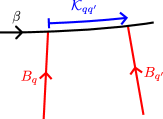
(a) $\epsilon=+$.

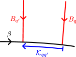
(b) $\epsilon=-$.

Figure 18. The segment $\mathcal{K}_{qq^{\prime}}$.

In the special case when a segment $\mathcal{K}_{qq^{\prime}}$ does not contain any other point $t(B_{q^{\prime\prime}})$ in its interior, with $B_{q^{\prime\prime}}$ also arriving on the same side as $B_{q}$ and $B_{q^{\prime}}$, then we simply denote by $\mathcal{K}_{q}$ this segment. This notation (where $q^{\prime}$ has been removed) is justified by the remark that there is exactly one $q^{\prime}$ with this property. We then denote $\tau_{q}:=\tau_{qq^{\prime}}$ (or, when convenient, $\tau(q)$).

4.3.2. Relation between $\tau$ and $\theta$

Each parameters $\tau_{qq^{\prime}}$ is a sum of a certain number of parameters $\theta_{q^{\prime\prime}}$: there exists a (uniquely defined) set of indices $\Theta_{\tau}(qq^{\prime})\subseteq\Theta$ such that

(4.13) $$\tau_{qq^{\prime}}=\sum_{q^{\prime\prime}\in\Theta_{\tau}(qq^{\prime})}\theta_{q^{\prime\prime}},$$

reflecting a partition of $\mathcal{K}_{qq^{\prime}}$ into $\mathcal{K}_{qq^{\prime}}=\bigsqcup_{q^{\prime\prime}\in\Theta_{\tau}(qq^{\prime})}\mathcal{I}_{q^{\prime\prime}}$.

In the case of $\tau_{q}$, we adopt as slightly simpler notation, writing that there exists a set of indices $\Theta_{\tau}(q)\subseteq\Theta$ such that

(4.14) $$\tau_{q}=\sum_{q^{\prime}\in\Theta_{\tau}(q)}\theta_{q^{\prime}}.$$

For a set $W\subseteq\Theta$, we let $\Theta_{\tau}(W):=\bigcup_{q\in W}\Theta_{\tau}(q)$. Note that this union is not necessarily disjoint.

4.4. Expression of the boundary lengths in the new coordinates

We are now ready to find the expression of the length of the curves $\Gamma_{\lambda}$ for $\lambda\in\Lambda$. We recall that we assumed, for the sake of simplicity, that the intersections have been opened the first way (see Remark 4.9 for the general case).

4.4.1. Case where $\Gamma_{\lambda}$ is a component of $\beta$

First, we note that in the special case where the curve $\Gamma_{\lambda}$ is a component of the multi-curve $\beta$, i.e. when $\lambda\in\Lambda^{\beta}$, then we can simply write $y_{\lambda}=\ell_{Y}(\beta_{\lambda})$, which has the simple expression in terms of the parameters $\vec{\theta}$:

(4.15) $$y_{\lambda}=\sum_{q:\lambda(q)=\lambda}\theta_{q}=\sum_{q\in\Theta_{t}(\lambda)}\theta_{q},$$

where we recall the definition of the set $\Theta_{t}(\lambda)$ from Notation 2.16.

4.4.2. Polygonal curve associated to $\Gamma_{\lambda}$

Let us now fix $\lambda\in\Lambda^{\Gamma}=\Lambda\setminus\Lambda^{\beta}$ (i.e. $\Gamma_{\lambda}$ is not a component of $\beta$). The length of $\Gamma_{\lambda}$ does not depend on its orientation; we orient it so that, if $j:=\operatorname{step}(\lambda)$ is the step of the construction of the pair of pants decomposition at which $\Gamma_{\lambda}$ appears, then $\mathbf{P}_{j}$ lies on the left of $\Gamma_{\lambda}$.

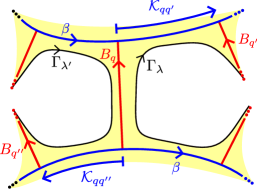
Figure 19. Following two (non-necessarily distinct) boundary components $\Gamma_{\lambda}$ and $\Gamma_{\lambda^{\prime}}$ of $\mathbf{S}$ near a bar $B_{q}$ with $\operatorname{Sign}(q)=+$.

Let us first assume that $\lambda\in\Lambda_{\mathrm{BC}}$, i.e. $\lambda$ is a boundary component of S. Examining the local picture at each intersection and following the boundary of the regular neighbourhood of the loop $\mathbf{c}$ (as represented in Figure 19), we obtain that we can write the boundary component $\Gamma_{\lambda}$ as an alternating succession of bars $B_{q}$ and segments $\mathcal{K}_{q}$ defined in §4.3, i.e. as

(4.16) $$\bar{p}_{1}^{\lambda}\mathord{\mathchoice{\,\vbox{\hbox{\scalebox{0.5}{$\displaystyle\bullet$}}}\,}{\,\vbox{\hbox{\scalebox{0.5}{$\textstyle\bullet$}}}\,}{\,\vbox{\hbox{\scalebox{0.5}{$\scriptstyle\bullet$}}}\,}{\,\vbox{\hbox{\scalebox{0.5}{$\scriptscriptstyle\bullet$}}}\,}}\ldots\mathord{\mathchoice{\,\vbox{\hbox{\scalebox{0.5}{$\displaystyle\bullet$}}}\,}{\,\vbox{\hbox{\scalebox{0.5}{$\textstyle\bullet$}}}\,}{\,\vbox{\hbox{\scalebox{0.5}{$\scriptstyle\bullet$}}}\,}{\,\vbox{\hbox{\scalebox{0.5}{$\scriptscriptstyle\bullet$}}}\,}}\bar{p}_{m(\lambda)}^{\lambda}$$

for some integer $m(\lambda)$, where each piece $\bar{p}_{k}^{\lambda}$ is a concatenation $\overline{B}_{q}\mathord{\mathchoice{\,\vbox{\hbox{\scalebox{0.5}{$\displaystyle\bullet$}}}\,}{\,\vbox{\hbox{\scalebox{0.5}{$\textstyle\bullet$}}}\,}{\,\vbox{\hbox{\scalebox{0.5}{$\scriptstyle\bullet$}}}\,}{\,\vbox{\hbox{\scalebox{0.5}{$\scriptscriptstyle\bullet$}}}\,}}\overline{\mathcal{K}}_{q}$ for some $q=q_{k}^{\lambda}\in\Theta$.

Remark 4.8.

We also notice that $\operatorname{Sign}q_{k}^{\lambda}=(-1)^{k}$, and in particular the integer $m(\lambda)$ is even, but this will not play any role in the discussion.

More generally, if $\lambda\in\Lambda_{\mathrm{in}}$, then we realise $\Gamma_{\lambda}$ as a boundary component of the surface $\mathbf{S}_{j}$ explored at the step $j$ of the construction of the pair of pants decomposition. We then obtain that $\Gamma_{\lambda}$ can, too, be written under the form (4.16), but now with bars $\bar{p}_{k}^{\lambda}=\overline{B}_{q}\mathord{\mathchoice{\,\vbox{\hbox{\scalebox{0.5}{$\displaystyle\bullet$}}}\,}{\,\vbox{\hbox{\scalebox{0.5}{$\textstyle\bullet$}}}\,}{\,\vbox{\hbox{\scalebox{0.5}{$\scriptstyle\bullet$}}}\,}{\,\vbox{\hbox{\scalebox{0.5}{$\scriptscriptstyle\bullet$}}}\,}}\overline{\mathcal{K}}_{qq^{\prime}}$ for some $q=q_{k}^{\lambda}$ and $q^{\prime}={q_{k}^{\prime\lambda}}\in\Theta$. See Figure 20 for an example.

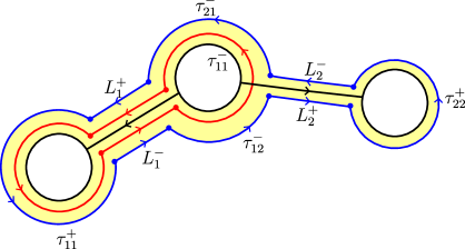
Figure 20. An example of the two new boundary components $\Gamma_{\lambda}$ for a case where $r=2$, and their description in terms of a succession of bars and segments $\mathcal{K}$. We use the shorthand notation $\tau_{ij}^{\epsilon}:=\tau_{(i,\epsilon),(j,\epsilon)}$.

This expression for the homotopy class of $\Gamma_{\lambda}$ is the equivalent of (4.3) for the curve $\mathbf{c}_{i}$ and will, as before, be our starting point to compute the length of $\Gamma_{\lambda}$. The lengths appearing in this decomposition are the lengths of the bars $\overline{B}_{q}$, which are the same lengths $L_{q}$ as before, now together with the lengths $\tau_{qq^{\prime}}$ of the segments $\overline{\mathcal{K}}_{qq^{\prime}}$.

The important observation here is that, as we go along the curve $\Gamma_{\lambda}$, we follow a succession of geodesic segments, only making right turns (as seen on Figure 19, and in the orientation convention of $\tau_{qq^{\prime}}$ in §4.3). Such a path will be called a polygonal curve in Definition 8.1.

Remark 4.9.

If we open the intersections both ways, we can still obtain a description of $\Gamma_{\lambda}$ as a polygonal curve (a succession of orthogonal geodesic segments making only right turns), but the notations for the orientations of the bars and the parameters $\tau$ need to be adapted. In particular, we no longer have alternate signs for the bars, and $m(\lambda)$ is not necessarily even (see for instance a figure-eight opened the second way).

4.4.3. Re-labelling

Let us now relabel the segments and lengths appearing in the decomposition (4.16) following the order in which they occur in $\Gamma_{\lambda}$. We shall therefore denote $\overline{B}^{\lambda}_{k}:=\overline{B}_{q_{k}^{\lambda}}$ and $\mathcal{K}^{\lambda}_{k}:=\mathcal{K}_{q_{k}^{\lambda}q_{k}^{\prime\lambda}}$, and call $L^{\lambda}_{k}$, $\tau^{\lambda}_{k}$ their respective lengths. Note that both these lengths are always positive quantities, by definition for $L^{\lambda}_{k}$, and in virtue of the Useful Remark for $\tau^{\lambda}_{k}$. We denote as $\vec{L}^{\lambda}$ and $\vec{\tau}^{\lambda}$ the vectors $\vec{L}^{\lambda}=(L_{1}^{\lambda},\ldots,L^{\lambda}_{m(\lambda)})$ and $\vec{\tau}^{\lambda}=(\tau^{\lambda}_{1},\ldots,\tau^{\lambda}_{m(\lambda)})$.

4.4.4. Expression of the length

We now follow quite closely the discussion of §4.1.

Lemma 4.10.

For any $Y\in\mathcal{T}_{g_{\mathbf{S}},n_{\mathbf{S}}}^{*}$, any $\lambda\in\Lambda^{\Gamma}$, we have

(4.17) $$\cosh\left(\frac{\ell_{Y}(\Gamma_{\lambda})}{2}\right)=\frac{1}{2}\,{{\rm Tr}\left(a_{1}^{\lambda}b_{1}^{\lambda}\ldots a_{m(\lambda)}^{\lambda}b_{m(\lambda)}^{\lambda}\right)}$$

where, for any index $k$, $a_{k}^{\lambda}:=A(L_{k}^{\lambda})$ and $b_{k}^{\lambda}:=A(\tau_{k}^{\lambda})$ with

(4.18) $$A(s):=w^{s}k^{-\frac{\pi}{2}}=\frac{\sqrt{2}}{2}\begin{pmatrix}e^{\frac{s}{2}}&-e^{-\frac{s}{2}}\\ e^{\frac{s}{2}}&e^{-\frac{s}{2}}\end{pmatrix}.$$

Proof.

The proof is the same as the proof of Lemma 4.3. The new path in $T^{1}\mathbf{S}$ that we consider is represented on Figure 21.

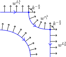
Figure 21. The path in $T^{1}\mathbf{S}$ followed in the proof of Lemma 4.10.

The key argument to remove the absolute value is that this path has the property required by Lemma 4.4, namely that the vectors always point to its left. ∎

Expanding the trace, we can deduce the following formula giving the lengths of the curves $\Gamma_{\lambda}$.

Theorem 4.11.

For any $Y\in\mathcal{T}_{g_{\mathbf{S}},n_{\mathbf{S}}}^{*}$, any $\lambda\in\Lambda^{\Gamma}$, we have

$$\cosh\left(\frac{\ell_{Y}(\Gamma_{\lambda})}{2}\right)=\frac{1}{2}\sum_{\alpha\in\{\pm 1\}^{m(\lambda)}}{\alpha_{1}\alpha_{2}\ldots\alpha_{m(\lambda)}}\operatorname{hyp}_{-\nabla\alpha}\left(\frac{L}{2}\right)\exp\left(\frac{\alpha\cdot\tau}{2}\right)$$

where $(\nabla\alpha)_{k}:=\alpha_{k}/{\alpha_{k-1}}=\alpha_{k}{\alpha_{k-1}}$ with the convention $\alpha_{0}=\alpha_{m(\lambda)}$.

Remark 4.12.

For $m=1$ this reduces to

$$\cosh\left(\frac{\ell_{Y}(\Gamma)}{2}\right)=\sinh\left(\frac{L_{1}}{2}\right)\sinh\left(\frac{\tau_{1}}{2}\right).$$

Proof.

To simplify notations, we shall remove the dependency on $\lambda$ from the name of the matrices and lengths. By equation (4.17), the announced quantity can be expressed as

$$\frac{1}{2}\,{{\rm Tr}\left(A(L_{1})A(\tau_{1})\ldots A(L_{m})A(\tau_{m})\right)}$$

where $A(s)$ is the matrix introduced in (4.18). Calculating the product, we find

$$A(L)A(\tau)=\begin{pmatrix}e^{\frac{\tau}{2}}\sinh\left(\frac{L}{2}\right)&-e^{-\frac{\tau}{2}}\cosh\left(\frac{L}{2}\right)\\ e^{\frac{\tau}{2}}\cosh\left(\frac{L}{2}\right)&-e^{-\frac{\tau}{2}}\sinh\left(\frac{L}{2}\right)\end{pmatrix}=\cosh\left(\frac{L}{2}\right)e_{-1}\left(\frac{\tau}{2}\right)+\sinh\left(\frac{L}{2}\right)e_{+1}\left(\frac{\tau}{2}\right)$$

with the matrices $e_{\pm 1}$ defined by

$$e_{+1}(s)=\begin{pmatrix}e^{s}&0\\ 0&-e^{-s}\end{pmatrix}\qquad\qquad e_{-1}(s)=\begin{pmatrix}0&-e^{-s}\\ e^{s}&0\end{pmatrix}.$$

We can use once again the matrices $E_{-1},E_{+1}$ introduced in equation (4.8), and note the relations

$$e_{+1}(s)e_{+1}(s^{\prime})=E_{+1}(s+s^{\prime})\qquad\qquad e_{+1}(s)e_{-1}(s^{\prime})=-E_{-1}(s-s^{\prime})$$

$$e_{-1}(s)e_{+1}(s^{\prime})=E_{-1}(-s-s^{\prime})\qquad\qquad e_{-1}(s)e_{-1}(s^{\prime})=-E_{+1}(s^{\prime}-s)$$

and

$$E_{+1}(s)e_{+1}(s^{\prime})=E_{-1}(s)e_{-1}(s^{\prime})=e_{+1}(s+s^{\prime})$$

$$E_{+1}(s)e_{-1}(s^{\prime})=E_{-1}(s)e_{+1}(s^{\prime})=e_{-1}(s^{\prime}-s).$$

A straightforward induction then shows that for any $s\in\mathbb{R}^{2k}$ and $\delta\in\{\pm 1\}^{2k}$,

$$e_{\delta_{1}}(s_{1})e_{\delta_{2}}(s_{2})\ldots e_{\delta_{2k}}(s_{2k})=\delta_{2}\delta_{4}\ldots\delta_{2k}\,E_{\pi(\delta)}(\alpha^{\delta}\cdot s),$$

where $\pi(\delta)=\prod_{k}\delta_{k}$ and $\alpha^{\delta}_{k}:=\prod_{j\leq k}\delta_{j}$, and that for any $s\in\mathbb{R}^{2k+1}$ and $\delta\in\{\pm 1\}^{2k+1}$,

$$e_{\delta_{1}}(s_{1})e_{\delta_{2}}(s_{2})\ldots e_{\delta_{2k+1}}(s_{2k+1})=\delta_{2}\delta_{4}\ldots\delta_{2k}\,e_{\pi(\delta)}(\pi(\delta)\,\alpha^{\delta}\cdot s).$$

Therefore, in the case $m=2k$,

$$\cosh\left(\frac{\ell(\Gamma)}{2}\right)=\frac{1}{2}\,\sum_{\delta\in\{\pm 1\}^{2k}}\delta_{2}\delta_{4}\ldots\delta_{m}\operatorname{hyp}_{-\delta}\left(\frac{L}{2}\right){\rm Tr}\left(E_{\pi(\delta)}\left(\frac{\alpha^{\delta}\cdot\tau}{2}\right)\right)$$

which implies that

$$\cosh\left(\frac{\ell(\Gamma)}{2}\right) =\sum_{\begin{subarray}{c}\delta\in\{\pm 1\}^{m}\\ \pi(\delta)=+1\end{subarray}}\delta_{2}\delta_{4}\ldots\delta_{m}\operatorname{hyp}_{-\delta}\left(\frac{L}{2}\right)\cosh\left(\frac{{\alpha^{\delta}\cdot\tau}}{2}\right)$$

since ${\rm Tr}(E_{+1}(s))=2\cosh(s)$ and ${\rm Tr}(E_{-1}(s))=0$. By expanding $\cosh\left(\frac{{\alpha^{\delta}\cdot\tau}}{2}\right)$ into exponential functions, and letting $\alpha_{k-1}\alpha_{k}=\delta_{k}=\alpha_{k}/\alpha_{k-1}$, we obtain the claimed formula.

In the case $m=2k+1$, we conclude similarly, now using

$$\cosh\left(\frac{\ell(\Gamma)}{2}\right) =\sum_{\begin{subarray}{c}\delta\in\{\pm 1\}^{m}\\ \pi(\delta)=+1\end{subarray}}\delta_{2}\delta_{4}\ldots\delta_{m-1}\operatorname{hyp}_{-\delta}\left(\frac{L}{2}\right)\sinh\left(\frac{{\alpha^{\delta}\cdot\tau}}{2}\right).$$

∎

4.4.5. Reformulation and final outcome

Motivated by Theorem 4.11, we now introduce the following notation.

Notation 4.13.

For an integer $m\geq 1$ and $x=(x_{1},\ldots,x_{m})$, $t=(t_{1},\ldots,t_{m})$, we define

(4.19) $$Q_{m}(x,t)=2\operatorname{argcosh}\frac{1}{2}\sum_{\alpha\in\{\pm 1\}^{m}}{\alpha_{1}\alpha_{2}\ldots\alpha_{m}}\operatorname{hyp}_{-\nabla\alpha}\left(\frac{x}{2}\right)\exp\left(\frac{\alpha\cdot t}{2}\right)$$

and

(4.20) $$F_{m}(x,t) =\frac{\cosh\Big{(}\frac{1}{2}Q_{m}(x,t)\Big{)}}{\exp\Big{(}\frac{1}{2}\sum_{n=1}^{m}t_{n}\Big{)}}=\frac{1}{2}\sum_{\alpha\in\{0,1\}^{m}}(-1)^{\alpha_{1}+\ldots+\alpha_{m}}\operatorname{hyp}_{-\partial\alpha}\left(\frac{x}{2}\right)\exp(-\alpha\cdot t)$$

with $(\partial\alpha)_{n}:=1$ if $\alpha_{n-1}=\alpha_{n}$ and $-1$ if $\alpha_{n-1}\not=\alpha_{n}$.

Remark 4.14.

Note that we go from (4.19) to (4.20) by the change of indices $(\alpha_{n})\rightsquigarrow(\frac{\alpha_{n}+1}{2})$.

We have proved that

(4.21) $$\ell_{Y}(\Gamma_{\lambda})=Q_{m(\lambda)}(\vec{L}^{\lambda},\vec{\tau}^{\lambda}).$$

We observe that the relation between the functions $Q_{m}$ and $F_{m}$ can be rewritten

(4.22) $$U(Q_{m}(x,t))=\sum_{n=1}^{m}t_{n}+2\log F_{m}(x,t),$$

for the function

(4.23) $$U(x)=2\log\cosh\left(\frac{x}{2}\right)=x-2\log 2+\mathcal{O}(e^{-x}).$$

The final outcome of the calculation then is

(4.24) $$\ell_{Y}(\Gamma_{\lambda})=\sum_{n=1}^{m(\lambda)}\tau^{\lambda}_{n}-2\log 2+2\log F_{m(\lambda)}(\vec{L}^{\lambda},\vec{\tau}^{\lambda})+\mathcal{O}(e^{-\ell_{Y}(\Gamma_{\lambda})}).$$

4.4.6. Set of indices associated to $\lambda$

Recall from (4.14) (the labelling by $q$ being replaced by $(\lambda,k)$) that the lengths $\tau^{\lambda}_{k}$ can be expressed by

(4.25) $$\tau^{\lambda}_{k}=\sum_{q\in\Theta_{\tau}(\lambda,k)}\theta_{q},$$

for some uniquely defined set of indices $\Theta_{\tau}(\lambda,k)\subseteq\Theta$. Now, we define the following index notation.

Notation 4.15.

For $\lambda\in\Lambda^{\Gamma}$, let

(4.26) $$\Theta_{\ell}(\lambda):=\bigcup_{k=1}^{m(\lambda)}\Theta_{\tau}(\lambda,k)\subseteq\Theta.$$

We extend the notation $\Theta_{\ell}(\lambda)$ to the indices $\lambda\in\Lambda^{\beta}$ by letting $\Theta_{\ell}(\lambda):=\Theta_{t}(\lambda)$ the set of indices introduced in Notation 2.16. If $W$ is a subset of $\Lambda$ we denote

(4.27) $$\Theta_{\ell}(W):=\bigcup_{\lambda\in W}\Theta_{\ell}(\lambda).$$

For any $\lambda\in\Lambda$, $\Theta_{\ell}(\lambda)$ denotes the set of indices $q\in\Theta$ necessary to express the length $\ell_{Y}(\Gamma_{\lambda})$.

Remark 4.16.

Keep in mind that the sets $\Theta_{\ell}(\lambda)$ are not disjoint: in fact, each $q\in\Theta$ may belong to two sets $\Theta_{\ell}(\lambda)$ with $\lambda\in\Lambda_{\mathrm{BC}}$, expressing the fact that each simple portion $\mathcal{I}_{q}$ has a boundary component of $\mathbf{S}$ on its left and one on its right. As a consequence, one has an inclusion $(\Theta_{\ell}(W))^{c}\subseteq\Theta_{\ell}(W^{c})$ (where $V^{c}$ denotes the complement of the set $V$), which in general is strict.

5. Expression of the volume functions as pseudo-convolutions of FR functions

Let us now, in this brief section, come back to our initial objective, i.e. proving Theorem 1.23, and reformulate it using the new notions and formulae presented in §2 to 4. More precisely, we shall explain how to compute the volume functions defined in (1.13) by

$$\mathcal{J}:\ell\mapsto\int_{\ell_{Y}({\mathbf{c}})=\ell}\prod_{j\in V}f_{j}(x_{j})\prod_{j=1}^{k}x_{i_{j}}\delta(x_{i_{j}}-x_{i_{j}^{\prime}})\frac{\,\mathrm{d}\mathrm{Vol}^{\mathrm{WP}}_{g_{\mathbf{S}},n_{\mathbf{S}}}(\mathbf{x},Y)}{\,\mathrm{d}\ell}$$

as pseudo-convolutions of functions in the class $\mathcal{F}$ – a notion that will be formalized in §6.

We recall that, in the integral above, $V$ is a subset of $\partial\mathbf{S}$. By our conventions introduced in §3.3, we identify $\partial\mathbf{S}$ with $\Lambda_{\mathrm{BC}}$, and hence $V$ with a subset of $\Lambda_{\mathrm{BC}}\subseteq\Lambda$. We write $V^{\beta}:=V\cap\Lambda^{\beta}$ and $V^{\Gamma}:=V\cap\Lambda^{\Gamma}$, so that $V^{\beta}$ are the components of $V$ that are components of the multi-curve $\beta$, and $V^{\Gamma}$ those that are not.

5.1. Change of variables

Let us change variables using our Jacobian computation, and more precisely its Dirac variant, Corollary 3.13. We obtain that:

$$\mathcal{J}(\ell)=2^{r}\int_{\ell_{Y}({\mathbf{c}})=\ell}{\mathchoice{1\mskip-4.0mu{\rm{l}}}{1\mskip-4.0mu{\rm{l}}}{1\mskip-4.5mu{\rm{l}}}{1\mskip-5.0mu{\rm{l}}}}_{\mathfrak{D}}(\vec{L},\vec{\theta})\prod_{\lambda\in V}f_{\lambda}(y_{\lambda})\frac{\prod_{\lambda\in V^{\beta}}\sinh\left(\frac{y_{\lambda}}{2}\right)\prod_{\lambda\in\Lambda_{\mathrm{in}}^{\beta}}\sinh^{2}\left(\frac{y_{\lambda}}{2}\right)}{\prod_{\lambda\in V^{\Gamma}}\sinh\left(\frac{y_{\lambda}}{2}\right)}\\ T_{V,\mathrm{m}}(\vec{L},\vec{\theta})\prod_{i=1}^{r}\sinh(L_{i})\frac{\,\mathrm{d}^{r}\vec{L}\,\mathrm{d}^{2r}\vec{\theta}}{\,\mathrm{d}\ell}$$

where $\mathfrak{D}$ is the domain of variation of the new variables $(\vec{L},\vec{\theta})$, studied in §3.5, and $T_{V,\mathrm{m}}$ is an explicit distribution which we shall leave as such. The integral $\mathcal{J}(\ell)$ can be rewritten under the simpler form

(5.1) $$\mathcal{J}(\ell)=2^{r}\int_{\ell_{Y}({\mathbf{c}})=\ell}{\mathchoice{1\mskip-4.0mu{\rm{l}}}{1\mskip-4.0mu{\rm{l}}}{1\mskip-4.5mu{\rm{l}}}{1\mskip-5.0mu{\rm{l}}}}_{\mathfrak{D}}(\vec{L},\vec{\theta})\prod_{\begin{subarray}{c}\lambda\in V^{\beta}_{+}\end{subarray}}g_{\lambda}(y_{\lambda})\prod_{\lambda\in V^{\Gamma}}u_{\lambda}(y_{\lambda})\,T_{V,\mathrm{m}}(\vec{L},\vec{\theta})\prod_{i=1}^{r}\sinh(L_{i})\frac{\,\mathrm{d}^{r}\vec{L}\,\mathrm{d}^{2r}\vec{\theta}}{\,\mathrm{d}\ell},$$

by setting $V^{\beta}_{+}:=V^{\beta}\cup\Lambda_{\mathrm{in}}^{\beta}$ and, for $\lambda\in\Lambda$,

$$g_{\lambda}(y):=f_{\lambda}(y)\sinh\left(\frac{y}{2}\right)\qquad\text{and}\qquad u_{\lambda}(y):=\frac{f_{\lambda}(y)}{\sinh\left(\frac{y}{2}\right)}$$

where $f_{\lambda}$ is already defined for $\lambda\in V\subseteq\Lambda_{\mathrm{BC}}$, and is extended to $\lambda\in\Lambda$ by letting

$$\begin{cases}f_{\lambda}(y):=1&\text{for }\lambda\in\Lambda_{\mathrm{BC}}\setminus V\\ f_{\lambda}(y):=\sinh\left(\frac{y}{2}\right)&\text{for }\lambda\in\Lambda_{\mathrm{in}}.\end{cases}$$

5.2. Expansion of the product in the integral

Let us now focus on the factor

(5.2) $$\prod_{\begin{subarray}{c}\lambda\in V^{\beta}_{+}\end{subarray}}g_{\lambda}(y_{\lambda})\prod_{V^{\Gamma}}u_{\lambda}(y_{\lambda})$$

appearing in the integral $\mathcal{J}$.

5.2.1. The functions $g_{\lambda}$

For technical considerations related to cancellations at zero in the integral, let us first rewrite for each $\lambda\in V^{\beta}_{+}$

$$g_{\lambda}(y):=\tilde{g}_{\lambda}(y)\chi_{\textrm{z}}(y)^{2},$$

where $\chi_{\textrm{z}}$ is the function introduced in Notation 1.22. We notice that we can apply the Friedman–Ramanujan hypothesis to every term $\tilde{g}_{\lambda}$ appearing in the product above. Indeed, for $\lambda\in V^{\beta}$, by the hypothesis on the functions $(f_{\lambda})_{\lambda\in V}$ in Notation 1.22, we have that $\tilde{g}_{\lambda}\in\mathcal{F}^{\mathrm{K}_{\lambda},\mathrm{N}_{\lambda}}$ and, if $p_{\lambda}$ denotes its principal term,

(5.3) $$|\tilde{g}_{\lambda}(y)-p_{\lambda}(y)\,e^{y}|\leq\|\tilde{g}_{\lambda}\|_{\mathcal{F}^{\mathrm{K}_{\lambda},\mathrm{N}_{\lambda}}}(1+y)^{\mathrm{N}_{\lambda}-1}e^{y/2}$$

where $p_{\lambda}$ is a polynomial of degree $\leq\mathrm{K}_{\lambda}-1$. For $\lambda\in\Lambda_{\mathrm{in}}^{\beta}$, we simply notice that $\tilde{g}_{\lambda}(y)=\sinh^{2}(y/2)/\chi_{\textrm{z}}(y)^{2}$ which belongs to $\mathcal{F}^{\mathrm{K}_{\lambda},\mathrm{N}_{\lambda}}$ for the integers $(\mathrm{K}_{\lambda},\mathrm{N}_{\lambda}):=(1,1)$, thanks to the fact that $\sinh^{2}(y/2)$ has a zero of order $2$ at $0$. Its principal term is $p_{\lambda}(y)e^{y}$ with $p_{\lambda}(y):=1/4$. We can write the Friedman–Ramanujan hypothesis explicitely for these terms and obtain

(5.4) $$|\tilde{g}_{\lambda}(y)-p_{\lambda}(y)\,e^{y}|\leq\|\tilde{g}_{\lambda}\|_{\mathcal{F}^{\mathrm{K}_{\lambda},\mathrm{N}_{\lambda}}}e^{y/2}$$

where $\|\tilde{g}_{\lambda}\|_{\mathcal{F}^{\mathrm{K}_{\lambda},\mathrm{N}_{\lambda}}}$ is a fixed universal constant.

We pick a set of indices $W^{\beta}\subseteq V^{\beta}_{+}$ for which we take the remainder term in the approximations (5.3) and (5.4). This allows us to expand the product as a sum of terms of the form

$$\prod_{\lambda\in V^{\beta}_{+}}\chi_{\textrm{z}}(y_{\lambda})^{2}\prod_{\lambda\in V^{\beta}_{+}\setminus W^{\beta}}p_{\lambda}(y_{\lambda})e^{y_{\lambda}}\prod_{\lambda\in W^{\beta}}\|\tilde{g}_{\lambda}\|_{\mathcal{F}^{\mathrm{K}_{\lambda},\mathrm{N}_{\lambda}}}\,r_{\lambda}(y_{\lambda})$$

where for all $\lambda\in W^{\beta}$, $|r_{\lambda}(y_{\lambda})|\leq(1+y_{\lambda})^{\mathrm{N}_{\lambda}-1}e^{y_{\lambda}/2}$.

We then use the fact that, for $\lambda\in\Lambda^{\beta}$, $y_{\lambda}$ is a linear combination of the components of the vector $\vec{\theta}$, given by the simple expression (4.15):

(5.5) $$y_{\lambda}=\sum_{q\in\Theta_{\ell}(\lambda)}\theta_{q}.$$

Note that the sets $\Theta_{\ell}(\lambda)$ for $\lambda\in V^{\beta}_{+}\setminus W^{\beta}$ are disjoint and their union is $\Theta_{\ell}(V^{\beta}_{+}\setminus W^{\beta})$ (note that this is not a priori the case for the sets $\Theta_{\ell}(\lambda)$ for $\lambda\in\Lambda$, and we here use the fact that $\lambda\in\Lambda^{\beta}$). We obtain that we can further expand the product as a sum of contribution of the form

(5.6) $$\mathrm{fn}((\tilde{g}_{\lambda})_{\lambda\in V^{\beta}})\prod_{\begin{subarray}{c}\lambda\in V^{\beta}_{+}\end{subarray}}\chi_{\textrm{z}}(y_{\lambda})^{2}\prod_{\lambda\in V^{\beta}_{+}\setminus W^{\beta}}\prod_{q\in\Theta_{\ell}(\lambda)}\theta_{q}^{\mathrm{K}_{q}^{\lambda}}\prod_{q\in\Theta_{\ell}(V^{\beta}_{+}\setminus W^{\beta})}e^{\theta_{q}}\prod_{\lambda\in W^{\beta}}r_{\lambda}(y_{\lambda})$$

where for $\lambda\in V^{\beta}_{+}\setminus W^{\beta}$, $\sum_{q\in\Theta_{\ell}(\lambda)}\mathrm{K}_{q}^{\lambda}\leq\mathrm{K}_{\lambda}-1$. In particular, for $\lambda\in\Lambda_{\mathrm{in}}^{\beta}$, $\mathrm{K}_{q}^{\lambda}=0$. We also note that the constant in front can be bounded by $\prod_{\lambda\in V^{\beta}}\|\tilde{g}_{\lambda}\|_{\mathcal{F}^{\mathrm{K}_{\lambda},\mathrm{N}_{\lambda}}}$.

5.2.2. The functions $u_{\lambda}$

Similarly, applying the Friedman–Ramanujan hypothesis to the functions $\tilde{g}_{\lambda}(y)=f_{\lambda}(y)\sinh(y/2)/\chi_{\textrm{z}}(y)^{2}\in\mathcal{F}^{\mathrm{K}_{\lambda},\mathrm{N}_{\lambda}}$ for $\lambda\in V^{\Gamma}$ allows us to replace the functions $u_{\lambda}$ by an approximation, this time by the polynomial function $p_{\lambda}$ coming from the principal term of $\tilde{g}_{\lambda}$, up to an exponentially decaying error. More precisely, using the relation

$$u_{\lambda}(y)=\frac{4\chi_{\textrm{z}}(y)^{2}}{(1-e^{-y})^{2}}e^{-y}\tilde{g}_{\lambda}(y)$$

together with the hypothesis (1.12) on the function $\chi_{\textrm{z}}$, we see that

$$|u_{\lambda}(y)-p_{\lambda}(y)|\leq 32\|\tilde{g}_{\lambda}\|_{\mathcal{F}^{\mathrm{K}_{\lambda},\mathrm{N}_{\lambda}}}(1+y)^{\mathrm{N}_{\lambda}-1}e^{-y/2}.$$

We now replace each term in the product by this expansion, and obtain it can be rewritten as a sum of terms of the form

$$\prod_{\lambda\in V^{\Gamma}\setminus W^{\Gamma}_{0}}p_{\lambda}(y_{\lambda})\prod_{\lambda\in W^{\Gamma}_{0}}32\|\tilde{g}_{\lambda}\|_{\mathcal{F}^{\mathrm{K}_{\lambda},\mathrm{N}_{\lambda}}}\,r_{\lambda}^{0}(y_{\lambda})$$

where $W^{\Gamma}_{0}\subseteq V^{\Gamma}$ and $|r_{\lambda}^{0}(y)|\leq(1+y)^{\mathrm{N}_{\lambda}-1}e^{-y/2}$ for all $\lambda\in W^{\Gamma}_{0}$.

We now express $p_{\lambda}(y_{\lambda})$ as a linear combination of monomials, and use the expression for $y_{\lambda}$ in terms of $(\vec{L},\vec{\theta})$ obtained in §4.4. Note that, for these terms which are not components of $\beta$, the expression is more complex, and not a simple linear combination. More precisely, by (4.24),

(5.7) $$y_{\lambda}=\sum_{n=1}^{m(\lambda)}\tau_{n}^{\lambda}-2\log 2+2\log F_{m(\lambda)}(\vec{L}^{\lambda},\vec{\tau}^{\lambda})+\mathcal{O}\left(e^{-y_{\lambda}}\right)$$

where $\vec{L}^{\lambda}=(L_{1}^{\lambda},\ldots,L_{m(\lambda)}^{\lambda})$ and $\vec{\tau}^{\lambda}=(\tau_{1}^{\lambda},\ldots,\tau_{m(\lambda)}^{\lambda})$ are the lengths of the bars and segments $\mathcal{K}$ appearing in the description of $\Gamma_{\lambda}$ as a polygonal curve, and $F_{m(\lambda)}$ is the function defined in (4.20). We can further express the parameters $\tau$ appearing in the sum in (5.7) in terms of $\vec{\theta}$ using (4.25) which states that

$$\tau_{n}^{\lambda}=\sum_{q\in\Theta_{\tau}(\lambda,n)}\theta_{q}.$$

The set of indices involved in writing $\vec{\tau}^{\lambda}$ is $\Theta_{\ell}(\lambda)=\bigcup_{n=1}^{m(\lambda)}\Theta_{\tau}(\lambda,n)$. Altogether, we obtain that the product of the $u_{\lambda}$ terms can be expressed as a sum of terms of the form

(5.8) $$\mathrm{fn}((\tilde{g}_{\lambda})_{\lambda\in V^{\Gamma}})\prod_{\lambda\in V^{\Gamma}\setminus W^{\Gamma}}\Big{[}(\log F_{m(\lambda)}(\vec{L}^{\lambda},\vec{\tau}^{\lambda}))^{d_{\lambda}}\prod_{q\in\Theta_{\ell}(\lambda)}\theta_{q}^{\mathrm{K}_{q}^{\lambda}}\Big{]}\prod_{\lambda\in W^{\Gamma}}r_{\lambda}(\vec{L},\vec{\theta}^{\lambda})$$

where:

• $W^{\Gamma}\subseteq V^{\Gamma}$ is the set of indices with exponential decay (it contains the set $W^{\Gamma}_{0}$ above, but can contain more elements due to the exponentially decaying term in (5.7));

• for $\lambda\in W^{\Gamma}$, $\vec{\theta}^{\lambda}=(\theta_{q})_{q\in\Theta_{\ell}(\lambda)}$ is the set of $\theta$ parameters required to express $y_{\lambda}$ and

  (5.9) $$|r_{\lambda}(\vec{L},\vec{\theta}^{\lambda})|\leq(1+y_{\lambda})^{\mathrm{N}_{\lambda}-1}e^{-y_{\lambda}/2};$$

• for $\lambda\in V^{\Gamma}\setminus W^{\Gamma}$, $\sum_{q\in\Theta_{\ell}(\lambda)}\mathrm{K}_{q}^{\lambda}+\,\mathrm{d}_{\lambda}\leq\mathrm{K}_{\lambda}-1$;

• the constant factor is bounded by $\prod_{\lambda\in V^{\Gamma}}\|\tilde{g}_{\lambda}\|_{\mathcal{F}^{\mathrm{K}_{\lambda},\mathrm{N}_{\lambda}}}$.

5.2.3. Conclusion and substitution in the integral

Taking equations (5.1), (5.6) and (5.8), we obtain that the integral $\mathcal{J}(\ell)$ can be rewritten as a fixed sum of terms of the form

(5.10) $$\begin{split}&\mathrm{fn}((\tilde{g}_{\lambda})_{\lambda\in V},r)\int_{\ell_{Y}(\mathbf{c})=\ell}{\mathchoice{1\mskip-4.0mu{\rm{l}}}{1\mskip-4.0mu{\rm{l}}}{1\mskip-4.5mu{\rm{l}}}{1\mskip-5.0mu{\rm{l}}}}_{\mathfrak{D}}(\vec{L},\vec{\theta})\prod_{\lambda\in V^{\beta}_{+}}\chi_{\textrm{z}}(y_{\lambda})^{2}\prod_{q\in\Theta_{\ell}(V_{+}\setminus W)}\theta_{q}^{\mathrm{K}_{q}}\prod_{q\in\Theta_{\ell}(V^{\beta}_{+}\setminus W^{\beta})}e^{\theta_{q}}\\ &\prod_{\lambda\in V^{\Gamma}\setminus W^{\Gamma}}(\log F_{m(\lambda)}(\vec{L}^{\lambda},\vec{\tau}^{\lambda}))^{d_{\lambda}}\prod_{\lambda\in W}r_{\lambda}(\vec{L},\vec{\theta}^{\lambda})\,T_{V,\mathrm{m}}(\vec{L},\vec{\theta})\prod_{i=1}^{r}\sinh(L_{i})\frac{\,\mathrm{d}^{r}\vec{L}\,\mathrm{d}^{2r}\vec{\theta}}{\,\mathrm{d}\ell},\end{split}$$

where:

• $V_{+}:=V\cup\Lambda_{\mathrm{in}}^{\beta}$ and $W:=W^{\beta}\cup W^{\Gamma}\subseteq V_{+}$;

• $\mathrm{K}_{q}:=\sum_{\lambda\in V_{+}\setminus W,\Theta_{\ell}(\lambda)\ni q}\mathrm{K}_{q}^{\lambda}$ (with $\mathrm{K}_{q}^{\lambda}$ defined to be $0$ if non already defined);

• $|r_{\lambda}(\vec{L},\vec{\theta}^{\lambda})|\leq(1+y_{\lambda})^{\mathrm{N}_{\lambda}-1}e^{\alpha_{\lambda}y_{\lambda}/2}$ with $\alpha_{\lambda}=1$ if $\lambda\in W^{\beta}$ and $-1$ if $\lambda\in W^{\Gamma}$

• the constant factor is bounded by $\mathrm{fn}(r)\prod_{\lambda\in V}\|\tilde{g}_{\lambda}\|_{\mathcal{F}^{\mathrm{K}_{\lambda},\mathrm{N}_{\lambda}}}$.

Note that we have

(5.11) $$\sum_{q\in\Theta_{\ell}(V_{+}\setminus W)}\mathrm{K}_{q}+\sum_{\lambda\in V^{\Gamma}\setminus W^{\Gamma}}d_{\lambda}\leq\sum_{\lambda\in V}(\mathrm{K}_{\lambda}-1).$$

5.3. Active and neutral parameters

Our final aim is to prove that the integral $\mathcal{J}$ is a Friedman–Ramanujan function following the method sketched in §1.3.8 to prove that a convolution $f_{1}\ast f_{2}$ is a Friedman–Ramanujan function. We recall that, in this case, the idea is to observe that $\mathcal{L}^{\mathrm{K}_{1}+\mathrm{K}_{2}}(f_{1}\ast f_{2})=\mathcal{L}^{\mathrm{K}_{1}}f_{1}\ast\mathcal{L}^{\mathrm{K}_{2}}f_{2}$. Hence, if we choose the indices $\mathrm{K}_{1}$ and $\mathrm{K}_{2}$ so that $\mathcal{L}^{\mathrm{K}_{i}}f_{i}$ are elements of $\mathcal{R}$ (which we can do if $f_{i}\in\mathcal{F}$), then we can easily deduce by an upper bound that $\mathcal{L}^{\mathrm{K}_{1}+\mathrm{K}_{2}}(f_{1}\ast f_{2})\in\mathcal{R}$, which in turn implies that $f_{1}\ast f_{2}\in\mathcal{F}$.

Now, if a function $f_{i}$ is already an element of $\mathcal{R}$, we do not need to cancel its principal term; in other words, we do not need to apply the operator $\mathcal{L}$ to $f_{i}$ in order to establish the Friedman–Ramanujan property for $f_{1}\ast f_{2}$ (we can take $\mathrm{K}_{i}=0$). In our language, this means that the variable $x_{i}$ corresponding to $f_{i}$ in the convolution $f_{1}\ast f_{2}(x)=\int_{x_{1}+x_{2}=x}f_{1}(x_{1})f_{2}(x_{2})\frac{\,\mathrm{d}x_{1}\,\mathrm{d}x_{2}}{\,\mathrm{d}x}$ is a neutral parameter. To the contrary, a variable which appears with a principal term in the integral (and will therefore need to be cancelled by applying the operator $\mathcal{L}$) will be called an active parameter.

Notation 5.1.

We partition the set of $\Theta$ into sets of active and neutral parameters $\Theta=\Theta_{\mathrm{ac}}\sqcup\Theta_{\mathrm{nt}}$ where

(5.12) $$\Theta_{\mathrm{ac}}:=\{q\in\Theta_{\ell}(V^{\beta}_{+})\,:\,q\notin\Theta_{\ell}(W)\}.$$

We denote as $\vec{\theta}_{\mathrm{ac}}=(\theta_{q})_{q\in\Theta_{\mathrm{ac}}}$ and $\vec{\theta}_{\mathrm{nt}}=(\theta_{q})_{q\in\Theta_{\mathrm{nt}}}$ the components of $\vec{\theta}=(\theta_{q})_{q\in\Theta}$ in those two sets of indices. We will call neutral parameters the components of $\vec{\theta}_{\mathrm{nt}}$ together with the vector $\vec{L}=(L_{1},\ldots,L_{r})$, and active parameters the components of $\vec{\theta}_{\mathrm{ac}}$.

In the following, the convolution argument will concern the variables $\vec{\theta}_{\mathrm{ac}}$, while $\vec{L}$ and $\vec{\theta}_{\mathrm{nt}}$ are kept fixed. We will not need to apply the operator $\mathcal{L}$ with respect to the neutral variables, because their contribution does not yield a principal term in the product (5.10).

Remark 5.2.

The reason why we do not need to work on the neutral parameters is that they will appear without a factor $2$ in our comparison estimate, Proposition 9.3. We have already commented on the importance of factors of $2$ in Proposition 1.30, a simple comparison estimate. We saw in Lemma 3.27 how double-filling loops (for which all parameters are neutral) can easily be proven to be Friedman–Ramanujan remainders, by direct inequalities, without any need to apply the operator $\mathcal{L}$.

We now set aside the neutral parameters in (5.10) and consider them as constants. The focus of the remainder of the paper is thus on integrals of the form

(5.13) $$\mathbf{Int}(\ell)=\int_{h(\vec{\theta}_{\mathrm{ac}})=\ell}\varphi_{0}(\vec{\theta}_{\mathrm{ac}})\prod_{q\in\Theta_{\mathrm{ac}}}\theta_{q}^{\mathrm{K}_{q}}e^{\theta_{q}}\,\frac{\,\mathrm{d}\vec{\theta}_{\mathrm{ac}}}{\,\mathrm{d}\ell}$$

where:

• all neutral variables $\vec{L},\vec{\theta}_{\mathrm{nt}}$ are fixed;

• we have the upper bound

  (5.14) $$\sum_{q\in\Theta_{\mathrm{ac}}}\mathrm{K}_{q}\leq\sum_{\begin{subarray}{c}\lambda\in V^{\beta}_{+}\\ \Theta_{\ell}(\lambda)\not\subseteq\Theta_{\ell}(W)\end{subarray}}(\mathrm{K}_{\lambda}-1)\leq\sum_{\lambda\in V^{\beta}_{+}\setminus W}(\mathrm{K}_{\lambda}-1);$$

• the weight function $\varphi_{0}$ is defined as

  (5.15) $$\varphi_{0}(\vec{\theta}_{\mathrm{ac}})={\mathchoice{1\mskip-4.0mu{\rm{l}}}{1\mskip-4.0mu{\rm{l}}}{1\mskip-4.5mu{\rm{l}}}{1\mskip-5.0mu{\rm{l}}}}_{\mathfrak{D}}(\vec{L},\vec{\theta})\prod_{\lambda\in V^{\beta}_{+}}\chi_{\textrm{z}}(y_{\lambda})^{2}\prod_{\lambda\in V^{\Gamma}\setminus W^{\Gamma}}(\log F_{m(\lambda)}(\vec{L}^{\lambda},\vec{\tau}^{\lambda}))^{d_{\lambda}}$$

  and, for each $\lambda\in V^{\Gamma}\setminus W^{\Gamma}$, $d_{\lambda}\leq\mathrm{K}_{\lambda}-1$;

• the level function $h$ is the length function of $\mathbf{c}$,

  (5.16) $$h(\vec{\theta}_{\mathrm{ac}})=\ell_{Y}({\mathbf{c}})=\sum_{i=1}^{\mathfrak{n}}\ell_{Y}({\mathbf{c}}_{i}).$$

It will be useful in the following to keep track of the quantities we have taken out of the integral due to depending only on neutral variables:

(5.17) $$\mathrm{fn}((\tilde{g}_{\lambda})_{\lambda\in V},r)\prod_{q\in\Theta_{\ell}(V_{+})\cap\Theta_{\mathrm{nt}}}\theta_{q}^{\mathrm{K}_{q}}\prod_{\lambda\in W}r_{\lambda}(\vec{L},\vec{\theta}_{\mathrm{nt}})\,T_{V,\mathrm{m}}(\vec{L},\vec{\theta}_{\mathrm{nt}})\prod_{i=1}^{r}\sinh(L_{i}).$$

Comparing with the forthcoming definition (6.3), this appears as the $(h,\varphi_{0})$-convolution of the Friedman–Ramanujan functions $(\theta_{q}^{\mathrm{K}_{q}}e^{\theta_{q}})_{q\in\Theta_{\mathrm{ac}}}$. The reason why we use the word convolution is that the function $h(\vec{\theta}_{\mathrm{ac}})$ behaves in many respects like the sum $\sum_{q\in\Theta_{\mathrm{ac}}}\theta_{q}$ (plus a function of the neutral variables), and the function $\varphi_{0}$ will be shown to have “small” derivatives in some sense, so it can be thought of as close to being constant. The purpose of §6 is to make these notions precise.

6. Pseudo-convolutions and stability of the FR hypothesis

In this section, we introduce a notion of pseudo-convolution $f_{1}\star\ldots\star f_{n}|^{h}_{\varphi}$ of functions $(f_{i})_{1\leq i\leq n}$ with the level function $h$ and the weight $\varphi$, which generalizes the usual convolution $f_{1}\ast\ldots\ast f_{n}$, and is motivated by the form of (5.13). We then study the way the operator $\mathcal{L}=\operatorname{id}-\mathcal{P}$ acts on pseudo-convolutions in §6.2. This will provide statements of the following kind: if $f_{1},\ldots,f_{n}$ are Friedman–Ramanujan functions, and if $(h,\varphi)$ satisfy adequate assumptions, then $f_{1}\star\ldots\star f_{n}|^{h}_{\varphi}$ is also a Friedman–Ramanujan function; see Theorem 6.28. Roughly speaking, the function $h(x_{1},\ldots,x_{n})$ is assumed to be close to $x_{1}+\ldots+x_{n}+C$ and $\varphi$ to a constant (in a certain topology defined in §6.3).

6.1. Definition of the notion of pseudo-convolution

We make the following definition.

Definition 6.1.

Take $n\geq 1$. Let $\varphi:\mathbb{R}^{n}\rightarrow\mathbb{R}$ be a locally bounded, measurable function, and $h$ be a real-valued mesurable function defined on a set containing the support $\operatorname{supp}(\varphi)$ of $\varphi$. We assume that for every compact subset $K\subset\mathbb{R}$, the set $h^{-1}(K)\cap\operatorname{supp}(\varphi)$ has finite measure.

We call $(h,\varphi)$-convolution of $n$ locally integrable functions $f_{1},\ldots,f_{n}:\mathbb{R}\rightarrow\mathbb{R}$ the pushforward of the product measure $\varphi(x_{1},\ldots,x_{n})\prod_{i=1}^{n}f_{i}(x_{i})\,\mathrm{d}x_{i}$ by the map $h$. In other words, it is the distribution $\nu$ on $\mathbb{R}_{\geq 0}$ defined by the fact that, for every continuous function $F:\mathbb{R}_{\geq 0}\rightarrow\mathbb{R}$ with compact support,

$$\int_{\mathbb{R}}F(x)\nu(\mathrm{d}x)=\int_{\mathbb{R}^{n}}F(h(x_{1},\ldots,x_{n}))\,\varphi(x_{1},\ldots,x_{n})\prod_{i=1}^{n}f_{i}(x_{i})\,\mathrm{d}x_{i}.$$

In our applications, the functions $h$ and $\varphi$ will always be much more than measurable. More precisely, throughout this article, we suppose the following.

Notation 6.2 (Assumptions on $(\varphi,h)$).

Take $a>0$. We assume the following.

• $\varphi:\mathbb{R}^{n}\rightarrow\mathbb{R}$ is a $\mathcal{C}^{1}$ function of support included in $(a,+\infty)^{n}$.

• $h:[a,+\infty)^{n}\rightarrow\mathbb{R}$ is a $\mathcal{C}^{1}$ function.

• For any index $1\leq i\leq n$ and any fixed $\hat{\mathbf{x}}_{i}=(x_{j})_{j\not=i}\in[a,+\infty)^{n-1}$, the function

  $$h_{i}^{\hat{\mathbf{x}}_{i}}:\,x_{i}\mapsto h(x_{1},\ldots,x_{n})$$

  is a $\mathcal{C}^{1}$-diffeomorphism from $[a,+\infty)$ onto its image; we denote $\ell\mapsto h_{i}^{-1}(\ell,\hat{\mathbf{x}}_{i})$ its inverse.

• The derivative $(\ell,\hat{\mathbf{x}}_{i})\mapsto\partial_{\ell}h_{i}^{-1}(\ell,\hat{\mathbf{x}}_{i})$ is bounded on its domain of definition.

The following proposition follows directly from the change of variable formula:

Proposition 6.3.

Under the hypotheses of Notation 6.2, the $(h,\varphi)$-convolution $\nu$ of any $n$ locally integrable functions $f_{1},\ldots,f_{n}$ admits a density with respect to the Lebesgue measure, with the following expression

(6.1) $$\frac{d\nu}{\,\mathrm{d}\ell}(\ell)=\int\varphi\big{(}x_{1},\ldots,h_{i}^{-1}(\ell,\hat{\mathbf{x}}_{i}),\ldots,x_{n}\big{)}f_{i}(h_{i}^{-1}(\ell,\hat{\mathbf{x}}_{i}))\prod_{j\not=i}f_{j}(x_{j})\,\partial_{\ell}h_{i}^{-1}(\ell,\hat{\mathbf{x}}_{i})\,\mathrm{d}\hat{\mathbf{x}}_{i}$$

where $\,\mathrm{d}\hat{\mathbf{x}}_{i}:=\prod_{j\not=i}\,\mathrm{d}x_{j}$. In particular this is independent of the choice of the index $i$.

Notation 6.4.

The expression (6.1) will be denoted $f_{1}\star\ldots\star f_{n}|^{h}_{\varphi}$.

If $x=(x_{1},\ldots,x_{n})$ are related by the implicit relation $h(x)=\ell$, we will denote $\frac{\,\mathrm{d}x_{1}\ldots\,\mathrm{d}x_{n}}{\,\mathrm{d}\ell}=\frac{\,\mathrm{d}x}{\,\mathrm{d}\ell}$ any of the equivalent expressions of the measure

(6.2) $$\frac{\,\mathrm{d}x_{1}\ldots\,\mathrm{d}x_{n}}{\,\mathrm{d}\ell}=\frac{\,\mathrm{d}x}{\,\mathrm{d}\ell}:=\partial_{\ell}h_{i}^{-1}(\ell,\hat{\mathbf{x}}_{i})\,\mathrm{d}\hat{\mathbf{x}}_{i}.$$

This corresponds to the disintegration of the Lebesgue measure $\,\mathrm{d}x=\,\mathrm{d}x_{1}\ldots\,\mathrm{d}x_{n}$ on the level-sets of $h$. Thus, we can write

(6.3) $$f_{1}\star\ldots\star f_{n}|^{h}_{\varphi}(\ell)= \int_{h(x)=\ell}\varphi(x)\prod_{i=1}^{n}f_{i}(x_{i})\,\frac{\,\mathrm{d}x}{\,\mathrm{d}\ell}.$$

Example 6.5.

The usual convolution corresponds to $h(x)=x_{1}+\ldots+x_{n}$, and either $\varphi\equiv 1$, or $\varphi(x)={\mathchoice{1\mskip-4.0mu{\rm{l}}}{1\mskip-4.0mu{\rm{l}}}{1\mskip-4.5mu{\rm{l}}}{1\mskip-5.0mu{\rm{l}}}}_{x_{1}\geq 0,\ldots,x_{n}\geq 0}$ (in the case of convolutions of functions defined on $\mathbb{R}_{\geq 0}$).

Remark 6.6 (Associativity).

The associativity of the usual convolution follows from associativity of the addition. For a general function $h$, the associativity rule may be replaced by formulae such as

$$f_{1}\star\ldots\star f_{n}|^{h}_{\varphi}(\ell)=\int f_{2}\star\ldots\star f_{n}|^{h_{x_{1}}}_{\varphi_{x_{1}}}(\ell)f_{1}(x_{1})\,\mathrm{d}x_{1}$$

where $\varphi_{x_{1}}$ (and similarly $h_{x_{1}}$) is the function of $n-1$ variables defined by freezing the first variable to $x_{1}$:

$$\varphi_{x_{1}}(x_{2},x_{3},\ldots,x_{n}):=\varphi(x_{1},x_{2},x_{3},\ldots,x_{n}).$$

This simply expresses the fact that we can do the convolution $f_{2}\star\ldots\star f_{n}|^{h_{x_{1}}}_{\varphi_{x_{1}}}$ with respect to $x_{2},\ldots,x_{n}$ (while $x_{1}$ is kept fixed) and then integrate with respect to $f_{1}(x_{1})\,\mathrm{d}x_{1}$, to obtain the pseudo-convolution $f_{1}\star\ldots\star f_{n}|^{h}_{\varphi}$.

In the rest of the article, we will need to use this associativity rule for multiple variables and pairs $(h,\varphi)$. In order to avoid cumbersome notations, we will often omit the index $x_{1}$ in the freezed functions $h_{x_{1}}$ and $\varphi_{x_{1}}$ when the context allows to avoid any confusion.

6.2. Action of the operator $\mathcal{L}_{\ell}$ on pseudo-convolution

In §1.3.7 we defined two operators acting on locally integrable functions, $\mathcal{P}_{x}=\int_{0}^{x}$ (taking a primitive) and $\mathcal{L}_{x}=\operatorname{id}-\mathcal{P}_{x}$. Since we are dealing with functions of several variables $(x_{1},\ldots,x_{n})$, the subscript $x_{i}$ will serve to indicate that the primitive is taken with respect to the variable $x_{i}$.

The goal of this section is to compare $\mathcal{L}^{\mathrm{K}_{1}+\ldots+\mathrm{K}_{n}}_{\ell}(f_{1}\star\ldots\star f_{n}|^{h}_{\varphi})$ with $(\mathcal{L}_{x_{1}}^{\mathrm{K}_{1}}f_{1})\star\ldots\star(\mathcal{L}_{x_{n}}^{\mathrm{K}_{n}}f_{n})|^{h}_{\varphi}$. With the usual convolution on functions defined on $\mathbb{R}$, we have the exact identity

(6.4) $$\mathcal{L}^{\mathrm{K}_{1}+\ldots+\mathrm{K}_{n}}_{\ell}(f_{1}*\ldots*f_{n})=(\mathcal{L}_{x_{1}}^{\mathrm{K}_{1}}f_{1})*\ldots*(\mathcal{L}_{x_{n}}^{\mathrm{K}_{n}}f_{n}).$$

Note that, in the case of functions defined on $\mathbb{R}_{\geq 0}$ only, there are additional boundary terms coming from $x_{i}=0$ in this relation (we leave this observation as an exercise to the reader).

For general functions $h$ and $\varphi$, the two expressions $\mathcal{L}^{\mathrm{K}_{1}+\ldots+\mathrm{K}_{n}}_{\ell}(f_{1}\star\ldots\star f_{n}|^{h}_{\varphi})$ and $(\mathcal{L}_{x_{1}}^{\mathrm{K}_{1}}f_{1})\star\ldots\star(\mathcal{L}_{x_{n}}^{\mathrm{K}_{n}}f_{n})|^{h}_{\varphi}$ will not be equal. We provide in Theorem 6.16 a detailed expression for the error term produced by replacing one by the other.

We saw in §1.3.8 how the identity (6.4) can be exploited to prove the stability of the Friedman–Ramanujan hypothesis by convolution. In §6.4, we will use the results of this section to provide a similar stability result, under certain hypotheses on the level function $h$ and the weight $\varphi$.

6.2.1. Basic calculus in one variable

We gather in the following lemmas the behavior of $\mathcal{P}$ and $\mathcal{L}$ under change of variables and multiplication. The change of variable formula yields:

Lemma 6.7.

Let $h:(0,+\infty)\rightarrow(h_{\inf},+\infty)$ be a $\mathcal{C}^{1}$-diffeomorphism with $h_{\inf}\geq 0$, and $h^{-1}$ be its inverse. Then, for any continuous function $G:\mathbb{R}_{\geq 0}\rightarrow\mathbb{R}$,

$$\mathcal{P}_{\ell}(G\circ h^{-1})=(\mathcal{P}_{x}G)\circ h^{-1}+R_{x}G\circ h^{-1}$$

where $R_{x}G(x):=\mathcal{P}_{x}(G(\partial_{x}h-1))$.

Proof.

This is just a way of writing

$$\int_{h_{\inf}}^{\ell}G(h^{-1}(u))\,\mathrm{d}u=\int_{0}^{h^{-1}(\ell)}G(t)\,\mathrm{d}t+\int_{0}^{h^{-1}(\ell)}G(t)(h^{\prime}(t)-1)\,\mathrm{d}t.$$

It is important to note that $\ell\mapsto G(h^{-1}(\ell))$ is only defined on $(h_{\inf},+\infty)$, so the operator $\mathcal{P}_{\ell}$ should, a priori, be defined as $\int_{h_{\inf}}^{\ell}$. However, if we extend $G(h^{-1}(\ell))$ to be $0$ if $\ell\leq h_{\inf}$, the formula remains true taking $\mathcal{P}_{\ell}=\int_{0}^{\ell}$. ∎

Integration by parts can be written in the following form:

Lemma 6.8.

For any continuous function $G:\mathbb{R}_{\geq 0}\rightarrow\mathbb{R}$ and any $\mathcal{C}^{1}$ function $\varphi:\mathbb{R}_{\geq 0}\rightarrow\mathbb{R}$,

$$\mathcal{P}_{x}(\varphi G)=\varphi\,\mathcal{P}_{x}G-\mathcal{P}_{x}\big{(}\partial_{x}{\varphi}\,\mathcal{P}_{x}G\big{)}.$$

Proof.

This just says that

$$\int_{0}^{x}\varphi(t)G(t)\,\mathrm{d}t=\varphi(x)\int_{0}^{x}G(t)\,\mathrm{d}t-\int_{0}^{x}\varphi^{\prime}(t)\Big{(}\int_{0}^{t}G(s)\,\mathrm{d}s\Big{)}\,\mathrm{d}t$$

which is indeed true by integration by parts. ∎

By combining both previous formulas and iterating them, we obtain:

Proposition 6.9.

With the notations of Lemma 6.7 and 6.8, for any $\mathrm{K}\geq 1$,

$$\mathcal{L}^{\mathrm{K}}_{\ell}((\varphi G)\circ h^{-1})=\, (\varphi\,\mathcal{L}^{\mathrm{K}}_{x}G)\circ h^{-1}$$

$$-\sum_{t=0}^{\mathrm{K}-1}\mathcal{L}_{\ell}^{\mathrm{K}-1-t}\big{(}(\varphi\,R_{x}(\mathcal{L}_{x}^{t}G))\circ h^{-1}\big{)}$$

$$+\sum_{t=0}^{\mathrm{K}-1}\mathcal{L}_{\ell}^{\mathrm{K}-1-t}\mathcal{P}_{\ell}\big{(}\partial_{\ell}(\varphi\circ h^{-1})\,\mathcal{P}_{\ell}(\mathcal{L}_{x}^{t}G\circ h^{-1})\big{)}.$$

Proof.

For $\mathrm{K}=1$, a combination of Lemmas 6.7 and 6.8 (w.r.t. the variable $\ell$) yields

$$\mathcal{L}_{\ell}((\varphi G)\circ h^{-1}) =(\varphi G)\circ h^{-1}-\mathcal{P}_{\ell}(\varphi\circ h^{-1}\cdot G\circ h^{-1})$$

$$\overset{\ref{l:product}}{=}(\varphi G)\circ h^{-1}-\varphi\circ h^{-1}\cdot\mathcal{P}_{\ell}(G\circ h^{-1})+\mathcal{P}_{\ell}\big{(}\partial_{\ell}(\varphi\circ h^{-1})\,\mathcal{P}_{\ell}(G\circ h^{-1})\big{)}$$

$$\overset{\ref{l:Icompo}}{=}(\varphi\,\mathcal{L}_{x}G)\circ h^{-1}-(\varphi\,R_{x}G)\circ h^{-1}+\mathcal{P}_{\ell}\big{(}\partial_{\ell}(\varphi\circ h^{-1})\,\mathcal{P}_{\ell}(G\circ h^{-1})\big{)}$$

which gives the expression of the commutator $[L,T]$ for with $L=\mathcal{L}$ and $TG=(\varphi G)\circ h^{-1}$:

$$[L,T]G=-(\varphi R_{x}G)\circ h^{-1}+\mathcal{P}_{\ell}\big{(}\partial_{\ell}(\varphi\circ h^{-1})\,\mathcal{P}_{\ell}(G\circ h^{-1})\big{)}.$$

We then use the algebraic identity

$$L^{\mathrm{K}}T=TL^{\mathrm{K}}+\sum_{t=0}^{\mathrm{K}-1}L^{\mathrm{K}-1-t}[L,T]L^{t}.$$

to obtain the claimed formula for general $\mathrm{K}$. ∎

6.2.2. Application to the first variable

Proposition 6.9 allows us to compare $\mathcal{L}_{\ell}^{\mathrm{K}}(f_{1}\star\ldots\star f_{n}|^{h}_{\varphi})$ with $(\mathcal{L}_{x_{1}}^{\mathrm{K}}f_{1})\star f_{2}\ldots\star f_{n}|^{h}_{\varphi}$, which is a first step towards the aim of this subsection. We prove the following.

Proposition 6.10.

For any family of continuous functions $(f_{j})_{1\leq j\leq n}$ and any integer $\mathrm{K}\geq 1$,

(6.5) $$\mathcal{L}_{\ell}^{\mathrm{K}}\big{(}f_{1}\star\ldots\star f_{n}|^{h}_{\varphi}\big{)}(\ell)= \;(\mathcal{L}_{x_{1}}^{\mathrm{K}}f_{1})\star f_{2}\star\ldots\star f_{n}|^{h}_{\varphi\frac{\partial h}{\partial x_{1}}}(\ell)+\mathcal{L}_{\ell}^{\mathrm{K}}\big{(}f_{1}\star\ldots\star f_{n}|^{h}_{\varphi(1-\frac{\partial h}{\partial x_{1}})}\big{)}(\ell)$$

(6.6) $$-\sum_{t=0}^{\mathrm{K}-1}\mathcal{L}_{\ell}^{\mathrm{K}-1-t}\Big{(}\int f_{2}\star\ldots\star f_{n}|^{h_{x_{1}}}_{\varphi\frac{\partial h}{\partial x_{1}}R_{x_{1}}(\mathcal{L}^{t}_{x_{1}}f_{1})}(\ell)\,\mathrm{d}x_{1}\Big{)}$$

(6.7) $$+\sum_{t=0}^{\mathrm{K}-1}\mathcal{L}_{\ell}^{\mathrm{K}-1-t}\mathcal{P}_{\ell}\Big{(}\int f_{2}\star\ldots\star f_{n}|^{h_{x_{1}}}_{\frac{\partial\varphi}{\partial x_{1}}\mathcal{P}_{x_{1}}(\mathcal{L}_{x_{1}}^{t}f_{1}\frac{\partial h}{\partial x_{1}})}(\ell)\,\mathrm{d}x_{1}\Big{)}.$$

Remark 6.11.

For the usual convolution, we have $h(x_{1},\ldots,x_{n})=x_{1}+\ldots+x_{n}$ and $\varphi=1$, so $\frac{\partial\varphi}{\partial x_{1}}=0$ and $\frac{\partial h}{\partial x_{1}}=1$ (and hence $R_{x_{1}}=0$). We see that only the first term remains:

$$\mathcal{L}_{\ell}^{\mathrm{K}}(f_{1}\ast\ldots\ast f_{n})=(\mathcal{L}_{x_{1}}^{\mathrm{K}}f_{1})\ast f_{2}\ast\ldots\ast f_{n}.$$

In the case $\varphi(x_{1},\ldots,x_{n})={\mathchoice{1\mskip-4.0mu{\rm{l}}}{1\mskip-4.0mu{\rm{l}}}{1\mskip-4.5mu{\rm{l}}}{1\mskip-5.0mu{\rm{l}}}}_{x_{1}\geq 0,\ldots,x_{n}\geq 0}$, we get a boundary term with a Dirac mass at $x_{1}=0$, it corresponds to the term (6.7).

Proof.

We start by writing our pseudo-convolution as:

(6.8) $$f_{1}\star\ldots\star f_{n}|^{h}_{\varphi}(\ell)=\int\varphi(h_{1}^{-1}(\ell,\hat{\mathbf{x}}_{1}),\hat{\mathbf{x}}_{1})\,f_{1}(h_{1}^{-1}(\ell,\hat{\mathbf{x}}_{1}))\prod_{i=2}^{n}f_{i}(x_{i})\,\partial_{\ell}h_{1}^{-1}(\ell,\hat{\mathbf{x}}_{1})\,\mathrm{d}x_{2}\ldots\,\mathrm{d}x_{n}.$$

We break (6.8) into two terms, writing

$$\partial_{\ell}h_{1}^{-1}(\ell,\hat{\mathbf{x}}_{1})=1+\partial_{\ell}h_{1}^{-1}(\ell,\hat{\mathbf{x}}_{1})\Big{(}1-\frac{\partial h}{\partial x_{1}}(h_{1}^{-1}(\ell,\hat{\mathbf{x}}_{1}))\Big{)}.$$

We observe that the second term on the right-hand-side yields exactly the second announced term in (6.5). We are therefore left to apply the operator $\mathcal{L}_{\ell}^{\mathrm{K}}$ to the function

$$\int\varphi(h_{1}^{-1}(\ell,\hat{\mathbf{x}}_{1}),\hat{\mathbf{x}}_{1})\,f_{1}(h_{1}^{-1}(\ell,\hat{\mathbf{x}}_{1}))\prod_{i=2}^{n}f_{i}(x_{i})\,\mathrm{d}x_{2}\ldots\,\mathrm{d}x_{n}$$

which we do by applying Proposition 6.9 with respect to the variable $x_{1}$ (while $x_{2},\ldots,x_{n}$ are frozen parameters) and the function $h=h_{1}$. We obtain:

(6.9) $$\mathcal{L}_{\ell}^{\mathrm{K}}\big{(}(\varphi f_{1})\circ h_{1}^{-1}\big{)}=\, \varphi\circ h_{1}^{-1}\,\big{(}\mathcal{L}^{\mathrm{K}}_{x_{1}}f_{1}\big{)}\circ h_{1}^{-1}$$

(6.10) $$-\sum_{t=0}^{\mathrm{K}-1}\mathcal{L}_{\ell}^{\mathrm{K}-1-t}\big{(}\varphi\circ h_{1}^{-1}\,\big{(}R_{x_{1}}(\mathcal{L}_{x_{1}}^{t}f_{1})\big{)}\circ h_{1}^{-1}\big{)}$$

(6.11) $$+\sum_{t=0}^{\mathrm{K}-1}\mathcal{L}_{\ell}^{\mathrm{K}-1-t}\mathcal{P}_{\ell}\big{(}\partial_{\ell}(\varphi\circ h_{1}^{-1})\,\mathcal{P}_{\ell}(\mathcal{L}_{x_{1}}^{t}f_{1}\circ h_{1}^{-1})\big{)}.$$

Integrating the terms (6.9) and (6.10) along $x_{2},\ldots,x_{n}$ respectively yield the first term of (6.5) and the term (6.6) in the theorem. For the last term (6.11), we use the chain rule

$$\partial_{\ell}(\varphi\circ h_{1}^{-1})=\Big{(}\frac{\partial\varphi}{\partial x_{1}}\circ h_{1}^{-1}\Big{)}\,\partial_{\ell}h_{1}^{-1},$$

and the change of variable

$$\mathcal{P}_{\ell}(\mathcal{L}_{x_{1}}^{t}f_{1}\circ h_{1}^{-1})=\mathcal{P}_{x_{1}}\Big{(}\mathcal{L}_{x_{1}}^{t}f_{1}\,\frac{\partial h}{\partial x_{1}}\Big{)}\circ h_{1}^{-1}$$

which leads to the claim once again by integration. ∎

Notation 6.12.

For $1\leq j\leq n$, $x=(x_{1},\ldots,x_{n})$ and $0\leq t\leq\mathrm{K}-1$, introduce the functions

$$F^{\mathrm{K}}_{j}(x)=\mathcal{L}_{x_{j}}^{\mathrm{K}}f_{j}(x_{j})\,\frac{\partial h}{\partial x_{j}}(x) G_{j}(x)=f_{j}(x_{j})\Big{(}1-\frac{\partial h}{\partial x_{j}}(x)\Big{)}$$

$$H^{t}_{j}(x)=-R_{x_{j}}(\mathcal{L}^{t}_{x_{j}}f_{j})(x_{j})\,\frac{\partial h}{\partial x_{j}}(x) I_{j}^{t}(x)=\mathcal{P}_{x_{j}}\Big{(}\mathcal{L}_{x_{j}}^{t}f_{j}\frac{\partial h}{\partial x_{j}}\Big{)}(x).$$

We can rephrase Proposition 6.10 as follows:

Corollary 6.13.

For any family of continuous functions $(f_{j})_{1\leq j\leq n}$ and any integer $\mathrm{K}\geq 1$, $\mathcal{L}_{\ell}^{\mathrm{K}}(f_{1}\star\ldots\star f_{n}|^{h}_{\varphi})$ is the sum of the following functions, or of the images of these functions under some power $\mathcal{L}_{\ell}^{t}$ where $0\leq t\leq\mathrm{K}-1$:

• $\int f_{2}\star\ldots\star f_{n}|^{h_{x_{1}}}_{T_{1}\varphi}(\ell)\,\mathrm{d}x_{1}$ where the operator $T_{1}$ is the multiplication by the function $F^{\mathrm{K}}_{1},G_{1}$ or $H_{1}^{t}$ with $0\leq t\leq\mathrm{K}-1$; or

• $\mathcal{P}_{\ell}\big{(}\int f_{2}\star\ldots\star f_{n}|^{h_{x_{1}}}_{T_{1}\varphi}(\ell)\,\mathrm{d}x_{1}\big{)}$ where $T_{1}=I_{1}^{t}\partial_{1}$ with $0\leq t\leq\mathrm{K}-1$, i.e. $T_{1}$ is the derivative with respect to $x_{1}$ followed by multiplication by $I_{1}^{t}$.

Proof.

We observe that by the associativity rule, Theorem 6.10 can also be written

$$\mathcal{L}_{\ell}^{\mathrm{K}}\big{(}f_{1}\star\ldots\star f_{n}|^{h}_{\varphi}\big{)}(\ell)= \;\int f_{2}\star\ldots\star f_{n}|^{h_{x_{1}}}_{F_{1}^{K}\varphi}(\ell)\,\mathrm{d}x_{1}+\mathcal{L}_{\ell}^{\mathrm{K}}\Big{(}\int f_{2}\star\ldots\star f_{n}|^{h_{x_{1}}}_{G_{1}\varphi}(\ell)\,\mathrm{d}x_{1}\Big{)}$$

$$+\sum_{t=0}^{\mathrm{K}-1}\mathcal{L}_{\ell}^{\mathrm{K}-1-t}\int f_{2}\star\ldots\star f_{n}(\ell)|^{h_{x_{1}}}_{H_{1}^{t}\varphi}\,\mathrm{d}x_{1}$$

$$+\sum_{t=0}^{\mathrm{K}-1}\mathcal{L}_{\ell}^{\mathrm{K}-1-t}\mathcal{P}_{\ell}\Big{(}\int f_{2}\star\ldots\star f_{n}|^{h_{x_{1}}}_{I_{1}^{t}\partial_{1}\varphi}(\ell)\,\mathrm{d}x_{1}\Big{)}.$$

The conclusion then follows directly. ∎

6.2.3. The multi-variable result

We shall now successively apply Corollary 6.13 in the variables $x_{1},\ldots,x_{n}$. In order to do so, the following notations for multi-indices will be helpful.

Notation 6.14 (Multi-indices).

If $\alpha=(\alpha_{1},\ldots,\alpha_{n})\in\mathbb{Z}_{\geq 0}^{n}$ is a multi-index, we use the standard notations $|\alpha|=\sum_{i=1}^{n}\alpha_{i}$, $\partial^{\alpha}=\prod_{i=1}^{n}\partial_{i}^{\alpha_{i}}$ (with $\partial_{i}=\frac{\partial}{\partial x_{i}}$) and $\alpha\cdot x=\sum_{i=1}^{n}\alpha_{i}x_{i}$.

Most of the time, all of the coefficients will be $\alpha_{i}=0$ or $1$, that is to say, we will manipulate differential operators of order at most one in each variable. This motivates the following convention.

Notation 6.15.

If $\pi$ is a subset of $\{1,\ldots,n\}$, we identify $\pi$ with the multi-index $\alpha={\mathchoice{1\mskip-4.0mu{\rm{l}}}{1\mskip-4.0mu{\rm{l}}}{1\mskip-4.5mu{\rm{l}}}{1\mskip-5.0mu{\rm{l}}}}_{\pi}$ (the indicator function of $\pi$), and hence denote $\partial^{\pi}=\partial^{{\mathchoice{1\mskip-4.0mu{\rm{l}}}{1\mskip-4.0mu{\rm{l}}}{1\mskip-4.5mu{\rm{l}}}{1\mskip-5.0mu{\rm{l}}}}_{\pi}}=\prod_{i\in\pi}\partial_{i}$. Then, ${\mathchoice{1\mskip-4.0mu{\rm{l}}}{1\mskip-4.0mu{\rm{l}}}{1\mskip-4.5mu{\rm{l}}}{1\mskip-5.0mu{\rm{l}}}}_{\pi}\cdot x=\sum_{i\in\pi}x_{i}$.

We now have the following.

Theorem 6.16.

For any family of continuous functions $(f_{j})_{1\leq j\leq n}$ and any integers $(\mathrm{K}_{j})_{1\leq j\leq n}$ with $\mathrm{K}_{j}\geq 1$, if $\mathrm{K}=\sum_{j=1}^{n}\mathrm{K}_{j}$, then the function $\mathcal{L}_{\ell}^{\mathrm{K}}(f_{1}\star\ldots\star f_{n}|^{h}_{\varphi})$ can be expressed as the sum of the following functions, or their images under $\mathcal{L}_{\ell}^{t}\mathcal{P}_{\ell}^{t^{\prime}}$ for $0\leq t\leq\mathrm{K}-n$ and $0\leq t^{\prime}\leq n$,

(6.12) $$\mathbf{Int}_{\pi}(\ell):=\int_{\begin{subarray}{c}h(x)=\ell\end{subarray}}\partial^{\pi_{0}}\varphi(x)\prod_{j=1}^{n}\partial^{\pi_{j}}\Phi_{j}(x)\frac{\,\mathrm{d}x}{\,\mathrm{d}\ell}$$

where:

• $\pi=(\pi_{j})_{0\leq j\leq n}$ is a family of disjoint subsets of $\{1,\ldots,n\}$ such that $j\notin\pi_{j}$ for all $j$;

• if $B:=\bigsqcup_{j=0}^{n}\pi_{j}$, then for any $1\leq j\leq n$,

  (6.13) $$\Phi_{j}=\begin{cases}F^{\mathrm{K}_{j}}_{j},G_{j}\text{ or }H_{j}^{t^{\prime\prime}}\text{ with }0\leq t^{\prime\prime}\leq\mathrm{K}_{j}-1&\text{if }j\not\in B\\ I_{j}^{t^{\prime\prime}}\text{ with }0\leq t^{\prime\prime}\leq\mathrm{K}_{j}-1&\text{if }j\in B.\end{cases}$$

Remark 6.17.

The set $B$ corresponds to the set of “bad” parameters, i.e. parameters for which $\Phi_{j}=I_{j}^{t^{\prime\prime}}$ (we will see in §6.4.2 why these terms are more problematic). It is also the set of variables w.r.t. which a derivative appears in (6.12).

Remark 6.18.

The number of possible terms of form (6.12) is $\mathrm{fn}(n,\mathrm{K})$.

The proof is an induction on the number of variables to which the operators are applied (Corollary 6.13 corresponding to one variable). More precisely, we prove the following result, and deduce Theorem 6.16 by taking $k=n$.

Lemma 6.19.

With the notations of Theorem 6.16, for any $k\in\{1,\ldots,n\}$, the function $\mathcal{L}_{\ell}^{\mathrm{K}_{1}+\ldots+\mathrm{K}_{k}}(f_{1}\star\ldots\star f_{n}|^{h}_{\varphi})$ can be expressed as the sum of the following functions, or their images under $\mathcal{L}_{\ell}^{t}\mathcal{P}_{\ell}^{t^{\prime}}$ for $0\leq t\leq\sum_{j=1}^{k}(\mathrm{K}_{j}-1)$ and $0\leq t^{\prime}\leq k$,

(6.14) $$\mathbf{Int}_{\pi}^{k}(\ell):=\int_{\begin{subarray}{c}h(x)=\ell\end{subarray}}\partial^{\pi_{0}}\varphi(x)\prod_{j=1}^{k}\partial^{\pi_{j}}\Phi_{j}(x)\prod_{j=k+1}^{n}f_{j}(x_{j})\frac{\,\mathrm{d}x}{\,\mathrm{d}\ell}$$

where:

• $\pi=(\pi_{j})_{0\leq j\leq k}$ is a family of disjoint subsets of $\{1,\ldots,k\}$ such that $\pi_{j}$ contains only integers $\geq j+1$ for all $j$;

• if $B:=\bigsqcup_{j=0}^{k}\pi_{j}$, then for any $1\leq j\leq k$, $\Phi_{j}$ satisfies (6.13).

Proof.

As announced, this is done by induction on $k$. For $k=1$, we see that the announced expression fits with Corollary 6.13. If $T_{1}$ is a multiplication operator by $\Phi_{1}\in\{F_{1}^{K_{1}},G_{1},H_{1}^{t^{\prime\prime}}\}$, we take $\pi_{0}=\pi_{1}=\emptyset$. If $T_{1}=I_{1}^{t^{\prime\prime}}\,\partial_{1}$, we take $\Phi_{1}=I_{1}^{t^{\prime\prime}}$, $\pi_{0}=\{1\}$ and $\pi_{1}=\emptyset$.

Assume the result is known for $k$. We apply Corollary 6.13 with respect to the variable $x_{k+1}$, to express the image under $\mathcal{L}^{\mathrm{K}_{k+1}}$ of the function (6.14), corresponding to a given data set $\pi=(\pi_{0},\ldots,\pi_{k})$. Application of Corollary 6.13 gives rise to four different kind of terms, depending on the nature of an operator $T_{k+1}$ that modifies the function under the integral. For the various situations, we examine how the data evolves to a new set of data $\pi^{\prime}=(\pi^{\prime}_{0},\pi^{\prime}_{1},\ldots,\pi^{\prime}_{k},\pi^{\prime}_{k+1})$, for which we check that the conditions of the theorem are still satisfied.

First, for the terms for which $T_{k+1}$ is a multiplication operator by a function $\Phi_{k+1}$ equal to $F^{\mathrm{K}_{k+1}}_{k+1}$, $G_{k+1}$ or $H_{k+1}^{t^{\prime\prime}}$, we take $\pi^{\prime}_{0}=\pi_{0}$, $\pi_{j}^{\prime}=\pi_{j}$ for $j\leq k$ and $\pi_{k+1}^{\prime}=\emptyset$.

The last terms are those for which $T_{k+1}=I_{k+1}^{t^{\prime\prime}}\partial_{{k+1}}$. We need to examine the effect of applying this operator to an expression of the form $\partial^{\pi_{0}}\varphi\prod_{j=1}^{k}\partial^{\pi_{j}}\Phi_{j}$. We use the Leibniz rule to write

(6.15) $$I_{k+1}^{t^{\prime\prime}}\partial_{{k+1}}\Big{(}\partial^{\pi_{0}}\varphi\prod_{j=1}^{k}\partial^{\pi_{j}}\Phi_{j}\Big{)}=I_{k+1}^{t^{\prime\prime}}\partial_{{k+1}}\partial^{\pi_{0}}\varphi\prod_{j=1}^{k}\partial^{\pi_{j}}\Phi_{j}+I_{k+1}^{t^{\prime\prime}}\partial^{\pi_{0}}\varphi\,\partial_{x_{k+1}}\Big{(}\prod_{j=1}^{k}\partial^{\pi_{j}}\Phi_{j}\Big{)}.$$

Then, we observe that those two terms can be expressed in the announced form, letting $\Phi_{k+1}=I_{k+1}^{t^{\prime\prime}}$, $\pi^{\prime}_{k+1}=\emptyset$, and

• for the first term, $\pi^{\prime}_{0}=\pi_{0}\cup\{k+1\}$ and $\pi^{\prime}_{j}=\pi_{j}$ for $1\leq j\leq k$;

• for the second term, we take $\pi^{\prime}_{0}=\pi_{0}$ and apply the Leibniz rule to the product $\prod_{j}\partial^{\pi_{j}}\Phi_{j}$, to write it as a sum of different contributions; then, for $1\leq j\leq k$, we take one of the $\pi^{\prime}_{j}$ to be equal to $\pi_{j}\cup\{k+1\}$ (corresponding to the index which is hit by the Leibniz rule) and leave all the others are untouched ($\pi^{\prime}_{j}=\pi_{j}$).

∎

6.3. The classes of functions $E^{(a)}$ and $\mathcal{E}^{(a)}$

Let us introduce classes of functions which will be helpful to quantify the distance between a $(h,\varphi)$ pseudo-convolution and the usual convolution.

6.3.1. Definition

For now, and the rest of the paper, we fix $a>0$.

Definition 6.20.

We let $E_{n}^{(a)}$ be the vector space of functions $h:[a,+\infty)^{n}\rightarrow\mathbb{R}$ such that:

• $h$ is of class $\mathcal{C}^{\infty}$;

• for every multi-index $\alpha\in\{0,1\}^{n}$ such that $\alpha\not=(0,\ldots,0)$,

  $$\sup_{x\in[a,+\infty)^{n}}\Big{\{}e^{\alpha\cdot x}|\partial^{\alpha}h(x)|\Big{\}}<+\infty.$$

This space is endowed with the seminorms $\lVert h\rVert_{\alpha,a}:=\sup\{e^{\alpha\cdot x}|\partial^{\alpha}h(x)|,x\in[a,+\infty)^{n}\}$.

Notice that, in this definition, we only control partial derivatives of $h$ that are of order at most one in each variable.

Notation 6.21.

Define $L_{n}(x_{1},\ldots,x_{n})=x_{1}+\ldots+x_{n}$ to be the linear functional associated to the usual convolution.

In what follows, we will prove results for pseudo-convolutions assuming that $h$ is close to $L_{n}$ in a certain sense; the definition below is used to quantify this.

Definition 6.22.

We let $\mathcal{E}_{n}^{(a)}$ be the affine space of functions $h$ such that $h-L_{n}\in E_{n}^{(a)}$. Equivalently, $h$ belongs in $\mathcal{E}_{n}^{(a)}$ if and only if

• $h$ is of class $\mathcal{C}^{\infty}$;

• for every multi-index $\alpha\in\{0,1\}^{n}$ such that $|\alpha|\geq 2$,

  $$\sup_{x\in[a,+\infty)^{n}}\Big{\{}e^{\alpha\cdot x}|\partial^{\alpha}h(x)|\Big{\}}<+\infty$$

• for every $j\in\{1,\ldots,n\}$,

  $$\sup_{x\in[a,+\infty)^{n}}\Big{\{}e^{x_{j}}|\partial_{j}h(x)-1|\Big{\}}<+\infty.$$

6.3.2. Core examples

Our main examples of such functions will be the following.

Notation 6.23.

For $\beta=(\beta_{\epsilon})_{\epsilon\in\{\pm\}^{n}}$ a family of real numbers, we define

$$h_{\beta}(x)=2\log\Big{(}\sum_{\epsilon\in\{\pm\}^{n}}\beta_{\epsilon}\operatorname{hyp}_{\epsilon}\left(\frac{x}{2}\right)\Big{)}.$$

Proposition 6.24.

We assume that $\beta$ is not identically $0$ and that, for all $\epsilon$, $\beta_{\epsilon}\geq 0$. Then, $h_{\beta}\in\mathcal{E}_{n}^{(a)}$ for any $a>0$. Moreover, there exists $C=C(a,n)$, independent of $\beta$, such that

(6.16) $$\sup_{\alpha\not=(0,\ldots,0)}\lVert h_{\beta}-L_{n}\rVert_{\alpha,a}\leq C.$$

Corollary 6.25.

The same result holds for the family

(6.17) $$\tilde{h}_{\beta}(x_{1},\ldots,x_{n})=2\operatorname{argcosh}\Big{(}\sum_{\epsilon\in\{\pm\}^{n}}\beta_{\epsilon}\operatorname{hyp}_{\epsilon}\left(\frac{x}{2}\right)\Big{)}$$

if we impose the additional condition that $\beta_{(1,\ldots,1)}\geq 1$.

Proof of Proposition 6.24.

For $y\in\mathbb{R}$, introduce

$$g_{\pm}(y)=e^{-y/2}\operatorname{hyp}_{\pm}(y)=\frac{1\pm e^{-y}}{2}.$$

Let $g_{\epsilon}(x)=\prod_{j=1}^{n}g_{\epsilon_{j}}(x_{j})$. We have

$$h_{\beta}(x)=L_{n}(x)+2\log\Big{(}\sum_{\epsilon\in\{\pm\}^{n}}\beta_{\epsilon}g_{\epsilon}(x)\Big{)}.$$

Note that $|\partial g_{+}(y)|=\frac{e^{-y}}{2}\leq e^{-y}g_{+}(y)$ and, if $y\geq a>0$,

$$|\partial g_{-}(y)|=\frac{e^{-y}}{2}\leq\frac{1}{1-e^{-a}}e^{-y}g_{-}(y).$$

It follows that the constant $C=(1-e^{-a})^{-n}$ satisfies, for all $\alpha\in\{0,1\}^{n}$ and $x\in[a,+\infty)^{n}$,

(6.18) $$|\partial^{\alpha}g_{\epsilon}(x)|\leq C\,e^{-\alpha\cdot x}g_{\epsilon}(x).$$

For $\alpha\in\{0,1\}^{n}$ with $|\alpha|=k\geq 1$, the partial derivative $\partial^{\alpha}\log\Big{(}\sum_{\epsilon\in\{\pm\}^{n}}\beta_{\epsilon}g_{\epsilon}(x)\Big{)}$ is a linear combination of terms of the form

(6.19) $$\frac{\prod_{j=1}^{k}\Big{(}\sum_{\epsilon\in\{\pm\}^{n}}\beta_{\epsilon}\partial^{\pi_{j}}g_{\epsilon}(x)\Big{)}}{\Big{(}\sum_{\epsilon\in\{\pm\}^{n}}\beta_{\epsilon}g_{\epsilon}(x)\Big{)}^{k}}$$

where $\pi_{1},\ldots,\pi_{k}$ form a partition of $\{i,\alpha_{i}=1\}$. For each $j\in\{1,\ldots,k\}$, (6.18) implies

$$\frac{\sum_{\epsilon\in\{\pm\}^{n}}\beta_{\epsilon}|\partial^{\pi_{j}}g_{\epsilon}(x)|}{\sum_{\epsilon\in\{\pm\}^{n}}\beta_{\epsilon}g_{\epsilon}(x)}\leq C\exp\Big{(}-\sum_{i\in\pi_{j}}\alpha_{i}x_{i}\Big{)}.$$

As a result, the term (6.19) is bounded by $C^{k}\exp(-\sum_{i=1}^{n}\alpha_{i}x_{i})$, proving the proposition. ∎

Let us now prove the corollary.

Proof of Corollary 6.25.

We write $\tilde{h}_{\beta}=V(h_{\beta})$ where

$$V(x)=2\operatorname{argcosh}(e^{\frac{x}{2}})=x+2\log 2+\omega(e^{-x})$$

is the reciprocal of the function $U$ that appeared in (4.22). By $\omega(e^{-x})$ we mean a function whose derivatives are all $\mathcal{O}(e^{-x})$. It is straightforward to check that $\tilde{h}$ satisfies the same derivative estimates as $h$, provided we know beforehand that $\sum_{\epsilon\in\{\pm\}^{n}}\beta_{\epsilon}\operatorname{hyp}_{\epsilon}\left(\frac{x}{2}\right)$ stays bounded away from $1$ on $[a,+\infty)^{n}$ (to avoid the singularity of $\operatorname{argcosh}$ at $1$). The condition $\beta_{(1,\ldots,1)}\geq 1$ implies that

$$\sum_{\epsilon\in\{\pm\}^{n}}\beta_{\epsilon}\operatorname{hyp}_{\epsilon}\left(\frac{x}{2}\right)\geq\exp\left(\frac{1}{2}\sum_{i=1}^{n}x_{i}\right)\geq\exp\Big{(}\frac{na}{2}\Big{)}>1$$

which is enough to conclude. ∎

6.3.3. Useful properties

First, we make the following immediate observation.

Remark 6.26.

If $\pi=(\pi_{1},\ldots,\pi_{N})$ is a partition of $\{1,\ldots,n\}$, and if for all $j\in\{1,\ldots,N\}$, the functions $(x_{i})_{i\in\pi_{j}}\mapsto h_{j}((x_{i})_{i\in\pi_{j}})$ are in $\mathcal{E}_{|\pi_{j}|}^{(a)}$, then following function is an element of $\mathcal{E}_{n}^{(a)}$:

$$(x_{1},\ldots,x_{n})\mapsto\sum_{j=1}^{N}h_{j}((x_{i})_{i\in\pi_{j}}).$$

It may also be useful to note the following simple implication of the definition of $\mathcal{E}_{n}^{(a)}$:

Proposition 6.27.

Assume that (6.16) holds for all $\alpha\in\{0,1\}^{n}$ such that $|\alpha|=1$. Then there exists $l_{0}\in\mathbb{R}$ such that, for all $x=(x_{1},\ldots,x_{n})\in[a,+\infty)^{n}$,

$$|h(x)-L_{n}(x)-l_{0}|\leq C\sum_{i=1}^{n}e^{-x_{i}}.$$

Proof.

First, we observe that if a function $g:[a,+\infty)\rightarrow\mathbb{R}$ satisfies $|g(t)-g(s)|\leq Ce^{-t}$ for all $t<s$, by Cauchy’s rule, it admits a limit $g(+\infty)$ at infinity, which satisfies

$$|g(t)-g(+\infty)|\leq Ce^{-t}.$$

This property holds for instance if $|g^{\prime}(t)|\leq Ce^{-t}$, and is stable under taking limits of sequences of functions. Applied to $g=h-L_{n}$ successively in each variable, denoting $l_{0}=g(+\infty,\ldots,+\infty)$, this yields

$$|g(x)-l_{0}| \leq\sum_{i=1}^{n}|g(x_{1},\ldots,x_{i-1},x_{i},+\infty,\ldots,+\infty)-g(x_{1},\ldots,x_{i-1},+\infty,+\infty,\ldots,+\infty)|$$

which implies that $|g(x)-l_{0}|\leq C\sum_{i=1}^{n}e^{-x_{i}}$. ∎

6.4. Stability of the Friedman–Ramanujan hypothesis by pseudo-convolution

We now have the ingredients to state a general result, according to which $f_{1}\star\ldots\star f_{n}|^{h}_{\varphi}$ is a Friedman–Ramanujan function if $f_{1},\ldots,f_{n}$ are so, under certain assumptions on $h$ on $\varphi$. In particular, we will prove Theorem 6.28 – which is not yet the result used to prove Theorem 1.23, but may be considered as a preliminary version, and provides a nice abstract statement:

Theorem 6.28.

Let $a>0$. We assume that $h\in\mathcal{E}_{n}^{(a)}$ and that $\varphi\in E_{n}^{(a)}$ with $\operatorname{supp}\varphi\subset(a,+\infty)^{n}$. If $(f_{j})_{1\leq j\leq n}$ are continuous functions in $\mathcal{F}$, then $f_{1}\star\ldots\star f_{n}|^{h}_{\varphi}\in\mathcal{F}$.

Recall that we always assume that the conditions of Notation 6.2 hold.

6.4.1. Quantitative hypotheses on the functions $h$, $\varphi$ and $f_{j}$

As we prove Theorem 6.28, we will be able to give estimates on the Friedman–Ramanujan norms of $f_{1}\star\ldots\star f_{n}|^{h}_{\varphi}$ as a function of those of $f_{1},\ldots,f_{n}$ (the precise bound is given in (6.27)). To this end, we introduce more specific notation which will be useful to track everything in the proof.

Notation 6.29.

Let $n\geq 1$ and $a>0$. We assume the following.

1. The function $h$ lies in $\mathcal{E}_{n}^{(a)}$. We denote $C_{1},C_{2}\geq 1$ two constants such that

   $$\forall\alpha\in\{0,1\}^{n}\setminus\{(0,\ldots,0)\}, \quad\lVert h-L_{n}\rVert_{\alpha,a}\leq C_{1}$$

   $$\forall j\in\{1,\ldots,n\}, \quad\Big{|}\frac{\partial h}{\partial x_{j}}\Big{|}\leq C_{2}.$$

   By the hypothesis from Notation 6.2 there exists a constant $C_{2}^{\prime}$ such that

   $$\forall j\in\{1,\ldots,n\},\quad 0<\Big{|}\frac{\partial x_{j}}{\partial h}\Big{|}\leq C_{2}^{\prime}.$$

   We let $C_{0}=\max(C_{1},C_{2},C_{2}^{\prime})$. By Proposition 6.27, there exists a $l_{0}\geq 1$ such that

   (6.20) $$\forall x=(x_{1},\ldots,x_{n})\in[a,+\infty)^{n},\quad\sum_{i=1}^{n}x_{i}\leq h(x)+l_{0}.$$

2. The function $\varphi$ is supported in $(a,+\infty)^{n}$ and $\varphi\in E_{n}^{(a)}$. Let $C_{3}\,\geq 0$ be a constant such that, for every multi-index $\alpha\in\{0,1\}^{n}$ with $\alpha\not=(0,\ldots,0)$, $\lVert\varphi\rVert_{\alpha,a}\leq C_{3}$.

3. For $j\in\{1,\ldots,n\}$, $f_{j}\in\mathcal{F}^{\mathrm{K}_{j},\mathrm{N}_{j}}$ is a continuous function. We assume w.l.o.g. that $\mathrm{K}_{j}\leq\mathrm{N}_{j}$ and $\lVert f_{j}\rVert_{\mathcal{F}^{\mathrm{K}_{j},\mathrm{N}_{j}}}=1$. By Remark 1.29, for $x_{j}\geq 0$ and $0\leq m<\mathrm{K}_{j}$,

   $$|\mathcal{L}^{m}f_{j}(x_{j})|\leq M_{\mathrm{K}_{j},\mathrm{N}_{j}}(1+x_{j})^{\mathrm{K}_{j}-1}e^{x_{j}}$$

   $$|\mathcal{L}^{\mathrm{K}_{j}}f_{j}(x_{j})|\leq M_{\mathrm{K}_{j},\mathrm{N}_{j}}(1+x_{j})^{\mathrm{N}_{j}-1}e^{\frac{x_{j}}{2}}.$$

   We let $\mathrm{K}=\sum_{j=1}^{n}\mathrm{K}_{j}$, $\mathrm{N}=\sum_{j=1}^{n}\mathrm{N}_{j}$ and $M_{\mathrm{K},\mathrm{N}}^{\times}:=\prod_{j=1}^{n}M_{\mathrm{K}_{j},\mathrm{N}_{j}}$.

Remark 6.30.

Comparison estimates such as (6.20), comparing $\sum_{i=1}^{n}x_{i}$ with $h(x_{1},\ldots,x_{n})$, are crucial throughout the paper.

6.4.2. Estimates on the functions $F_{j}^{\mathrm{K}_{j}}$, $G_{j}$, $H_{j}^{t}$ and $I_{j}^{t}$

We can deduce from our hypotheses some bounds on the functions introduced in Notation 6.12, which appear when computing $\mathcal{L}^{\mathrm{K}}_{\ell}(f_{1}\star\ldots f_{n}|_{\varphi}^{h})$. This will allow us to foresee some key elements of the proof of Theorem 6.28.

Lemma 6.31.

Under the assumptions ($h$) and ($f$) from Notation 6.29, for $j\in\{1,\ldots,n\}$, for any set $\pi_{j}\subset\{1,\ldots,n\}$ such that $j\notin\pi_{j}$ and any $x\in[a,+\infty)^{n}$,

• if $\Phi_{j}=F^{\mathrm{K}_{j}}_{j},G_{j}$ or $H_{j}^{t}$ with $0\leq t<\mathrm{K}_{j}$,

  (6.21) $$|\partial^{\pi_{j}}\Phi_{j}(x)|\leq C_{0}^{2}M_{\mathrm{K}_{j},\mathrm{N}_{j}}(1+x_{j})^{\mathrm{N}_{j}}e^{\frac{x_{j}}{2}}\prod_{i\in\pi_{j}}e^{-x_{i}}$$

• if $\Phi_{j}=I_{j}^{t}$ with $0\leq t<\mathrm{K}_{j}$,

  (6.22) $$|\partial^{\pi_{j}}\Phi_{j}(x)|\leq C_{0}^{2}M_{\mathrm{K}_{j},\mathrm{N}_{j}}(1+x_{j})^{\mathrm{N}_{j}}e^{x_{j}}\prod_{i\in\pi_{j}}e^{-x_{i}}.$$

Proof.

If $\pi_{j}=\emptyset$, it is a straightforward computation that

$$\begin{cases}|F^{\mathrm{K}_{j}}_{j}(x)|\leq C_{2}M_{\mathrm{K}_{j},\mathrm{N}_{j}}(1+x_{j})^{\mathrm{N}_{j}-1}e^{\frac{x_{j}}{2}},\\ |G_{j}(x)|\leq C_{1}M_{\mathrm{K}_{j},\mathrm{N}_{j}}(1+x_{j})^{\mathrm{K}_{j}-1},\\ |H^{t}_{j}(x)|\leq C_{1}C_{2}M_{\mathrm{K}_{j},\mathrm{N}_{j}}(1+x_{j})^{\mathrm{K}_{j}}\end{cases}$$

and

$$|I^{t}_{j}(x)|\leq C_{2}M_{\mathrm{K}_{j},\mathrm{N}_{j}}(1+x_{j})^{\mathrm{K}_{j}-1}e^{x_{j}}.$$

We then use the fact that $\mathrm{K}_{j}\leq\mathrm{N}_{j}$ and $C_{1},C_{2}\leq C_{0}$. When $\pi_{j}$ is non-empty, the additional exponential factors come from the hypothesis on the derivatives of $h$. ∎

We here see the crucial phenomenon at play for the proof of Theorem 6.28: compared to the original upper bound $|f_{j}(x_{j})|\leq M_{\mathrm{K}_{j},\mathrm{N}_{j}}(1+x_{j})^{\mathrm{K}_{j}-1}e^{x_{j}}$, we have gained in (6.21) a factor $e^{-x_{j}/2}$ when replacing the function $f_{j}$ by the function $F^{\mathrm{K}_{j}}_{j}$, $G_{j}$ or $H^{t}_{j}$. Unfortunately, the estimate we obtain on the function $I^{t}_{j}$ does not constitute an improvement compared to the initial growth-rate of $f_{j}$.

In this case however, an exponential factor $e^{-x_{j}/2}$ will be gained elsewhere, from the derivatives of the other functions. Remember that we have noticed in Remark 6.17 that the set of “bad” indices $B$ for which the function $I_{j}^{t}$ appears corresponds to the set of derivatives that appear elsewhere in the integral. We have seen in the lemma above that such derivatives will create a decay reducing the growth of $I_{j}^{t}$.

We obtain the following bound on the quantity $\mathcal{L}^{\mathrm{K}}(f_{1}\star\ldots\star f_{n}\|^{h}_{\varphi})$.

Proposition 6.32.

Under the assumptions ($h$) and ($f$) from Notation 6.29,

(6.23) $$|\mathcal{L}^{\mathrm{K}}(f_{1}\star\ldots\star f_{n}\|^{h}_{\varphi})(\ell)|\leq\sum_{\pi}\sum_{0\leq t+t^{\prime}\leq\mathrm{K}}|\mathcal{L}_{\ell}^{t}\mathcal{P}_{\ell}^{t^{\prime}}\mathbf{Int}_{\pi}(\ell)|$$

and

(6.24) $$|\mathbf{Int}_{\pi}(\ell)|\leq C_{0}^{2n}M_{\mathrm{K},\mathrm{N}}^{\times}\int_{\begin{subarray}{c}h(x)=\ell\end{subarray}}|\partial^{\pi_{0}}\varphi(x)|\prod_{j\in B\setminus\pi_{0}}e^{-x_{j}}\prod_{j\in B}(1+x_{j})^{\mathrm{N}_{j}}e^{x_{j}}\prod_{j\not\in B}(1+x_{j})^{\mathrm{N}_{j}}e^{\frac{x_{j}}{2}}\frac{\,\mathrm{d}x}{\,\mathrm{d}\ell}.$$

Proof.

The bound (6.23) is a direct consequence of the expression (6.12) together with the triangle inequality. Recall that

$$\mathbf{Int}_{\pi}(\ell)=\int_{h(x)=\ell}\partial^{\pi_{0}}\varphi(x)\prod_{j=1}^{n}\partial^{\pi_{j}}\Phi_{j}(x)\,\frac{\,\mathrm{d}x}{\,\mathrm{d}\ell}$$

where $\pi_{0},\pi_{1},\ldots,\pi_{n}$ are disjoint subsets of $\{1,\ldots,n\}$ such that $j\notin\pi_{j}$, and $B=\bigsqcup_{j=0}^{n}\pi_{j}$. We then use Lemma 6.31 on each term, remembering that $\Phi_{j}$ is in the first situation if $j\notin B$ and the second if $j\in B$. We conclude by noticing that $\prod_{j=1}^{n}\prod_{i\in\pi_{j}}e^{-x_{i}}=\prod_{j\in B\setminus\pi_{0}}e^{-x_{j}}$. ∎

Remark 6.33.

The previous statement is not completely optimal, but we have decided to line up all the estimates on the worst possible case. For later use, it will also be useful to lose again in optimality in (6.24), and write that:

(6.25) $$\begin{split}|\mathbf{Int}_{\pi}(\ell)|\leq C_{0}^{2n}M^{\times}_{\mathrm{K},\mathrm{N}}\int_{\begin{subarray}{c}h(x)=\ell\end{subarray}}|\partial^{\pi_{0}}\varphi(x)|\prod_{\begin{subarray}{c}j\notin\pi_{0}\end{subarray}}e^{-\frac{x_{j}}{2}}\prod_{j=1}^{n}(1+x_{j})^{\mathrm{N}_{j}}e^{x_{j}}\frac{\,\mathrm{d}x}{\,\mathrm{d}\ell}.\end{split}$$

If we compare with (6.24), we note that we have accepted to waste a factor $e^{-\frac{x_{j}}{2}}$ for $j\in B\setminus\pi_{0}$. The resulting upper bound only depends on $\pi_{0}$ and not on $B$ (both coincide if $\pi_{0}=B$).

6.4.3. End of the proof of Theorem 6.28

We are now ready to finish the proof of Theorem 6.28 by using Assumption ($\varphi$) to bound (6.24).

Proof.

Given that we now assume that $|\partial^{\pi_{0}}\varphi(x)|\leq C_{3}e^{-\sum_{j\in\pi_{0}}x_{j}}$, we obtain that for any term $\pi$ in (6.23),

(6.26) $$|\mathbf{Int}_{\pi}(\ell)|\leq C_{3}\,C_{0}^{2n}M^{\times}_{\mathrm{K},\mathrm{N}}\int_{h(x)=\ell}\prod_{j=1}^{n}(1+x_{j})^{\mathrm{N}_{j}}e^{\frac{x_{j}}{2}}\frac{\,\mathrm{d}x}{\,\mathrm{d}\ell}.$$

We now explicit the level-set integration and use the comparison estimate (6.20). We obtain that

$$|\mathbf{Int}_{\pi}(\ell)|\leq C_{3}\,C_{0}^{2n}M^{\times}_{\mathrm{K},\mathrm{N}}\int_{\sum_{j=2}^{n}x_{j}\leq\ell+l_{0}}\prod_{j=1}^{n}(1+x_{j})^{\mathrm{N}_{j}}e^{\frac{x_{j}}{2}}\Big{|}\frac{\partial x_{1}}{\partial h}\Big{|}\prod_{j=2}^{n}\,\mathrm{d}x_{j}$$

which, by assumption on the inverse derivatives of $h$, implies

$$|\mathbf{Int}_{\pi}(\ell)|\leq C_{3}\,C_{0}^{2n}C_{2}^{\prime}M^{\times}_{\mathrm{K},\mathrm{N}}(1+\ell+l_{0})^{\mathrm{N}}e^{\frac{\ell+l_{0}}{2}}\int_{\sum_{j=2}^{n}x_{j}\leq\ell+l_{0}}\prod_{j=2}^{n}\,\mathrm{d}x_{j}.$$

As a consequence,

$$|\mathbf{Int}_{\pi}(\ell)|\leq C_{3}\,C_{0}^{2n+1}M^{\times}_{\mathrm{K},\mathrm{N}}(1+\ell+l_{0})^{\mathrm{N}+n-1}e^{\frac{\ell+l_{0}}{2}}.$$

We have thus proven that the functions $\mathbf{Int}_{\pi}$ are in the class $\mathcal{R}^{\mathrm{N}+n}$. From Proposition 6.32, $\mathcal{L}_{\ell}^{\mathrm{K}}(f_{1}\star\ldots\star f_{n}|^{h}_{\varphi})$ is a sum of such functions (or images thereof under powers of $\mathcal{P}_{\ell}$ or $\mathcal{L}_{\ell}$), hence $\mathcal{L}_{\ell}^{\mathrm{K}}(f_{1}\star\ldots\star f_{n}|^{h}_{\varphi})\in\mathcal{R}^{\mathrm{N}+n}$. Proposition 1.27 then implies that $f_{1}\star\ldots\star f_{n}|^{h}_{\varphi}$ belongs in $\mathcal{F}^{\mathrm{K},\mathrm{N}+n}$. The proof furthermore gives

(6.27) $$\lVert f_{1}\star\ldots\star f_{n}|^{h}_{\varphi}\rVert_{\mathcal{F}^{\mathrm{K},\mathrm{N}+n}}\leq C_{3}\,C_{0}^{2n+1}\mathrm{fn}(n,\mathrm{K})(1+l_{0})^{\mathrm{N}+n-1}e^{\frac{l_{0}}{2}}\prod_{j=1}^{n}\lVert f_{j}\rVert_{\mathcal{F}^{\mathrm{K}_{j},\mathrm{N}_{j}}}.$$

∎

6.5. Problems in the geometric application of Assumption ($h$) and ($\varphi$)

Having noticed at the end of §5 that the integral (5.13) is the $(h,\varphi_{0})$-convolution of Friedman–Ramanujan functions (with $\varphi_{0}$ and $h$ specified in (5.15) and (5.16) respectively), we now need to examine the possibility to apply Theorem 6.28. Unfortunately, the functions $h$ and $\varphi_{0}$ do not satisfy the required assumptions, which explains why we will need two additional sections §7 and §8 to solve these issues.

6.5.1. Problem with Assumption ($h$)

The explicit expression of $\ell_{Y}({\mathbf{c}})$ was obtained in (4.12). By virtue of Corollary 6.25 and Remark 6.26, for each parameter $\vec{L}$, we have that the function

$$h:\vec{\theta}\mapsto\ell_{Y}({\mathbf{c}})$$

lies in the set $\mathcal{E}^{(a)}_{2r}$ provided we restrict all the $\theta_{q}$ to be $\geq a$. If we now fix the neutral parameters $\vec{\theta}_{\mathrm{nt}}\in\mathbb{R}_{\geq 0}^{\Theta_{\mathrm{nt}}}$ and consider

(6.28) $$h:\vec{\theta}_{\mathrm{ac}}\mapsto\ell_{Y}({\mathbf{c}}),$$

then it is easy to check that the restriction of this function to $\mathbb{R}_{\geq a}^{\Theta_{\mathrm{ac}}}$ belongs to $\mathcal{E}^{(a)}_{\#\Theta_{\mathrm{ac}}}$.

We have already remarked that the non-crossing variables $\theta_{q}$ stay positive, as consequence of the Useful Remark 2.11. As a consequence, in the purely non-crossing case (when all variables are non-crossing), Assumption ($h$) is satisfied.

If there exists some crossing variables, then they may take positive or negative values, in which case we are out of the domain of application of Corollary 6.25.

$\rightsquigarrow$Section 7 will be devoted to solving this issue by choosing a different representative of the homotopy class of ${\mathbf{c}}$. This will provide an expression of $h$ which falls in a class $\mathcal{E}$ with respect to newly defined variables. The reader might wish to focus upon first read on the purely non-crossing case, and hence skip §7.2 and §7.3.

6.5.2. Problem with Assumption ($\varphi$)

The coefficients arising in the expression of $Q_{m(\lambda)}$, obtained in (4.19) and (4.21), are equal to $\pm 1$, thus not of constant sign. As a consequence, we cannot use Proposition 6.24 nor Corollary 6.25 to deduce that $Q_{m(\lambda)}$ belongs to the class $\mathcal{E}_{m(\lambda)}$ with respect to the variables $(\tau^{\lambda}_{1},\ldots,\tau^{\lambda}_{m(\lambda)})$. We cannot either deduce that the functions $\log F_{m(\lambda)}$ are in the class $E_{m(\lambda)}$.

$\rightsquigarrow$ Section §8 will be devoted to estimating the derivatives of $F_{m(\lambda)}$. Again this will necessitate changing the representative of the homotopy class of $\Gamma_{\lambda}$.

6.6. Variants of Theorem 6.28

In the geometric applications of these techniques, we shall not use Theorem 6.28 directly, but several variants. Because these variants become quite technical, we present them by gradually modifying the assumptions and conclusions. The reader is invited to skip this section at first read, and come back to it when the necessity for these variants becomes clear.

6.6.1. First variant: comparison estimates

First, we loosen the decay hypothesis on $\varphi$, and replace it by a new assumption.

Notation 6.34 (Assumption ($\varphi$-CE)).

Assume that the smooth function $\varphi$ is supported on $(a,+\infty)^{n}$ and there exists positive functions $Z_{j}:\mathbb{R}_{>0}\rightarrow\mathbb{R}_{>0}$, $1\leq j\leq n$, such that:

• for all $\pi_{0}\subseteq\{1,\ldots,n\}$, all $x=(x_{1},\ldots,x_{n})\in(a,+\infty)^{n}$,

  $$|\partial^{\pi_{0}}\varphi(x)|\leq C_{3}\,\prod_{j\in\pi_{0}}\frac{1}{Z_{j}^{1/2}(x_{j})};$$

• there exists $l_{0}>0$ satisfying (6.20) and such that, for any $\pi_{0}\subseteq\{1,\ldots,n\}$,

  (6.29) $$2\sum_{j=1}^{n}x_{j}\leq h(x)+\sum_{j\not\in\pi_{0}}x_{j}+\sum_{j\in\pi_{0}}\log Z_{j}+l_{0}.$$

The important point, here, is that the functions $(Z_{j})_{1\leq j\leq n}$ controlling the decay of the derivatives of $\varphi$ can be incorporated in a comparison estimate for the function $h$.

Remark 6.35.

The initial result, Theorem 6.28, may be recovered by taking $Z_{j}=e^{x_{j}}$, in which case the comparison estimate (6.29) coincides with (6.20).

Theorem 6.36.

Let $a>0$. We assume that the assumptions ($h$), ($f$) and ($\varphi$-CE) hold. Then, $f_{1}\star\ldots\star f_{n}|^{h}_{\varphi}\in\mathcal{F}^{\mathrm{K},\mathrm{N}+n}$, and the estimate (6.27) holds.

Proof.

We do not reproduce the proof, completely identical to the proof of Theorem 6.28. A crucial point is again the comparison estimate (6.29), which may be rewritten on the level-set $\{h(x)=\ell\}$ in exponential form

$$\prod_{j=1}^{n}e^{x_{j}}\prod_{j\in\pi_{0}}\frac{1}{Z_{j}^{1/2}}\prod_{j\not\in\pi_{0}}e^{-\frac{x_{j}}{2}}\leq e^{\frac{l_{0}}{2}}e^{\frac{\ell}{2}}.$$

This means that the gain $\prod_{j\in\pi_{0}}Z_{j}^{-1/2}\prod_{j\not\in\pi_{0}}e^{-x_{j}/2}$ on the left-hand side results in a growth of size $e^{\ell/2}$ instead of the expected $e^{\ell}$ on the right-hand side, leading to the fact that the resulting function is a Friedman–Ramanujan remainder. ∎

6.6.2. Second variant: Linear forms

In our geometric applications, $\varphi(x_{1},\ldots,x_{n})$ will actually be split into a product involving linear forms, as follows:

Notation 6.37.

Let $\varphi$ be of the form:

(6.30) $$\varphi(x_{1},\ldots,x_{n})=\phi(\tau_{1},\ldots,\tau_{m})\,\psi(x_{1},\ldots,x_{n})$$

where, for all $1\leq i\leq m$, $\tau_{i}$ is a linear form, and more precisely $\tau_{i}(x)=\sum_{j\in\Theta(i)}x_{j}$ for a subset $\Theta(i)\subseteq\{1,\ldots,n\}$. For $\tilde{\pi}\subseteq\{1,\ldots,m\}$, we denote $\Theta(\tilde{\pi}):=\bigcup_{i\in\tilde{\pi}}\Theta(i)$.

Remark 6.38.

The original result corresponds to the case where $m=n$, $\Theta(i)=\{i\}$ so that $\tau_{i}(x)=x_{i}$, and $\psi=1$.

Let us adapt Theorem 6.16 to this new form of the density $\varphi$. The motivation for this upcoming variant may be roughly explained as follows: suppose that the derivatives $\partial^{\tilde{\pi}}\phi(\tau_{1},\ldots,\tau_{m})$ are bounded by

(6.31) $$|\partial^{\tilde{\pi}}\phi(\tau_{1},\ldots,\tau_{m})|\leq C_{3}\,e^{-\sum_{i\in\tilde{\pi}}\tau_{i}}=C_{3}\,e^{-\sum_{i\in\tilde{\pi}}\sum_{j\in\Theta(i)}x_{j}}$$

for any $\tilde{\pi}\subseteq\{1,\ldots,m\}$. Then, once the term $\partial^{\tilde{\pi}}\phi$ appears in the application of Corollary 6.13, there is no further need to gain exponential decay with respect to the variables $x_{j}$ with $j\in\Theta(\tilde{\pi})$. We wish to avoid this extra work, not only to optimize the proof, but also because in the geometric application the higher order derivatives of $\phi$ will be difficult to calculate. Thus, we copy the proof of Theorem 6.16, but once $\phi$ has been differentiated with respect to a variable $x_{j}$ (say, for $j\in\Theta(i)$), we stop applying our operators to the other variables $x_{j^{\prime}}$ with $j^{\prime}\in\Theta(i)$. This leads to the following statement.

Theorem 6.39.

For any family of continuous functions $(f_{j})_{1\leq j\leq n}$ and any integers $(\mathrm{K}_{j})_{1\leq j\leq n}$ with $\mathrm{K}_{j}\geq 1$, if $\mathrm{K}=\sum_{j=1}^{n}\mathrm{K}_{j}$, then the function $\mathcal{L}_{\ell}^{\mathrm{K}}(f_{1}\star\ldots\star f_{n}|^{h}_{\varphi})$ can be expressed as the sum of the following functions, or their images under $\mathcal{L}_{\ell}^{t}\mathcal{P}_{\ell}^{t^{\prime}}$ for $0\leq t\leq\mathrm{K}-n$ and $0\leq t^{\prime}\leq n$,

(6.32) $$\mathbf{Int}_{\tilde{\pi}_{0},\tilde{\pi},\mathcal{V},\pi}(\ell):=\int_{\begin{subarray}{c}h(x)=\ell\end{subarray}}\partial^{\tilde{\pi}}\phi(\tau_{1},\ldots,\tau_{m})\,\partial^{\pi_{0}}\psi(x)\prod_{j\in\mathcal{V}}\partial^{\pi_{j}}\Phi_{j}(x)\prod_{j\notin\mathcal{V}}f_{j}(x_{j})\frac{\,\mathrm{d}x}{\,\mathrm{d}\ell}$$

where:

• $\tilde{\pi}_{0}\subseteq\{1,\ldots,n\}$ and $\tilde{\pi}\subseteq\{1,\ldots,m\}$ are two sets of same cardinal, with a bijection $\tilde{\pi}_{0}\ni j\mapsto i_{j}\in\tilde{\pi}$ such that $j\in\Theta(i_{j})$ for all $j\in\tilde{\pi}_{0}$;

• $\mathcal{V}$ is a subset of $\{1,\ldots,n\}$ containing $\tilde{\pi}_{0}$, and so that $\mathcal{V}\cup\Theta(\tilde{\pi})=\{1,\ldots,n\}$;

• $(\pi_{j})_{j\in\mathcal{V}\cup\{0\}}$ is a family of disjoint subsets of $\mathcal{V}\setminus\tilde{\pi}_{0}$ such that $j\notin\pi_{j}$ for all $j$;

• if $B:=\tilde{\pi}_{0}\sqcup\pi_{0}\sqcup\bigsqcup_{j\in\mathcal{V}}\pi_{j}$, then for any $j\in\mathcal{V}$, $\Phi_{j}$ satisfies (6.13).

Remark 6.40.

To go from Theorem 6.39 to Theorem 6.16, let $\tilde{\pi}_{0}=\tilde{\pi}=\emptyset$, $\mathcal{V}=\{1,\ldots,n\}$.

We prove, once again, this result by proving the following (stronger) lemma for by induction on the integer $0\leq k\leq n$. This leads to the claim taking $k=n$.

Lemma 6.41.

For any $0\leq k\leq n$, the function $\mathcal{L}_{\ell}^{\mathrm{K}}(f_{1}\star\ldots\star f_{n}|^{h}_{\varphi})$ can be expressed as the sum of the following functions, or their images under $\mathcal{L}_{\ell}^{t}\mathcal{P}_{\ell}^{t^{\prime}}$ for $0\leq t\leq\mathrm{K}-k$ and $0\leq t^{\prime}\leq k$,

(6.33) $$\mathbf{Int}_{\tilde{\pi}_{0},\tilde{\pi},\mathcal{V},\pi}^{k}(\ell):=\int_{\begin{subarray}{c}h(x)=\ell\end{subarray}}\partial^{\tilde{\pi}}\phi(\tau_{1},\ldots,\tau_{m})\,\partial^{\pi_{0}}\psi(x)\prod_{j\in\mathcal{V}}\partial^{\pi_{j}}\Phi_{j}(x)\prod_{j\notin\mathcal{V}}f_{j}(x_{j})\frac{\,\mathrm{d}x}{\,\mathrm{d}\ell}$$

where:

• $\tilde{\pi}_{0}\subseteq\{1,\ldots,k\}$ and $\tilde{\pi}\subseteq\{1,\ldots,m\}$ are two sets of same cardinal, with a bijection $\tilde{\pi}_{0}\ni j\mapsto i_{j}\in\tilde{\pi}$ such that $j\in\Theta(i_{j})$ for all $j\in\tilde{\pi}_{0}$;

• $\mathcal{V}$ is a subset of $\{1,\ldots,k\}$ containing $\tilde{\pi}_{0}$, and so that $\{1,\ldots,k\}\subseteq\mathcal{V}\cup\Theta(\tilde{\pi})$;

• $(\pi_{j})_{j\in\mathcal{V}\cup\{0\}}$ is a family of disjoint subsets of $\mathcal{V}\setminus\tilde{\pi}_{0}$ such that $\pi_{j}$ contains only integers $\geq j+1$ for all $j$;

• if $B:=\tilde{\pi}_{0}\sqcup\pi_{0}\sqcup\bigsqcup_{j\in\mathcal{V}}\pi_{j}$, then for any $j\in\mathcal{V}$, $\Phi_{j}$ satisfies (6.13).

Proof.

For $k=0$, we take $\tilde{\pi}=\tilde{\pi}_{0}=\pi_{0}=\mathcal{V}=\emptyset$. Now assume the formula known at rank $k$ and let us prove it for $k+1$, by applying $\mathcal{L}^{\mathrm{K}_{k+1}}$ to an expression of the form (6.33).

First, let us observe that, if $k+1\in\Theta(\tilde{\pi})$, then we can simply apply $\mathcal{L}^{\mathrm{K}_{k+1}}$ to the integral (6.32) and leave it unchanged; the result will satisfy the requirements of the theorem at the rank $k+1$, with the same $\tilde{\pi}_{0}$, $\tilde{\pi}$, $\mathcal{V}$, $(\pi_{j})_{j\in\mathcal{V}}$.

Let us now assume that $k+1\notin\Theta(\tilde{\pi})$. As before, we apply Corollary 6.13 to (6.33) with respect to the variable $x_{{k+1}}$. For each term, we explicit how the data $(\tilde{\pi}_{0},\tilde{\pi},\mathcal{V},(\pi_{j})_{j\in\mathcal{V}})$ evolves to a new set of data $(\tilde{\pi}_{0}^{\prime},\tilde{\pi}^{\prime},\mathcal{V}^{\prime},(\pi_{j}^{\prime})_{j\in\mathcal{V}^{\prime}})$ which satifies the conditions at the next rank. Note that, here, we will always take $\mathcal{V}^{\prime}=\mathcal{V}\cup\{k+1\}$ and $\pi_{k+1}^{\prime}=\emptyset$.

In the three first cases, $T_{k+1}$ is a multiplication operator by some function $\Phi_{k+1}$ equal to $F^{\mathrm{K}_{{k+1}}}_{{k+1}}$, $G_{{k+1}}$ or $H_{{k+1}}^{t}$. We take $\tilde{\pi}_{0}^{\prime}=\tilde{\pi}_{0}$, $\tilde{\pi}^{\prime}=\tilde{\pi}$, and $\pi_{j}^{\prime}=\pi_{j}$ for $j\in\mathcal{V}$.

Otherwise, $T_{k+1}=I_{{k+1}}^{t}\partial_{{k+1}}$. In this case, we let $\Phi_{{{k+1}}}=I_{{k+1}}^{t}$. When we apply $\partial_{k+1}$ to an expression of the form $\partial^{\tilde{\pi}}\phi(\tau_{1},\ldots,\tau_{m})\,\partial^{\pi_{0}}\psi(x)\prod_{j\in\mathcal{V}}\partial^{\pi_{j}}\Phi_{j}(x)$ and then multiply it by $I_{k+1}^{t}=\partial^{\pi_{k+1}^{\prime}}\Phi_{k+1}$, by the Leibniz rule we obtain three types of terms.

• Terms of the form

  (6.34) $$\partial^{\tilde{\pi}}\partial_{{i}}\phi(\tau_{1},\ldots,\tau_{m})\,\partial^{\pi_{0}}\psi(x)\prod_{j\in\mathcal{V}^{\prime}}\partial^{\pi_{j}}\Phi_{j}(x)$$

  for $i\in\{1,\ldots,m\}$ with $k+1\in\Theta(i)$. We note that by hypothesis $i\notin\tilde{\pi}$. We take $\tilde{\pi}_{0}^{\prime}=\tilde{\pi}_{0}\cup\{k+1\}$, $\tilde{\pi}^{\prime}=\tilde{\pi}\cup\{i\}$, and leave the $(\pi_{j})_{j\in\mathcal{V}}$ unchanged.

• A term of the form

  (6.35) $$\partial^{\tilde{\pi}}\phi(\tau_{1},\ldots,\tau_{m})\;\partial^{\pi_{0}}\partial_{{k+1}}\psi(x)\prod_{j\in\mathcal{V}^{\prime}}\partial^{\pi_{j}}\Phi_{j}(x)$$

  for which we set $\tilde{\pi}_{0}^{\prime}=\tilde{\pi}_{0}$, $\tilde{\pi}^{\prime}=\tilde{\pi}$, $\pi_{0}^{\prime}=\pi_{0}\cup\{k+1\}$, and leave the $(\pi_{j})_{j\in\mathcal{V}}$ unchanged.

• Finally, a term of the form

  (6.36) $$\partial^{\tilde{\pi}}\phi(\tau_{1},\ldots,\tau_{m})\;\partial^{\pi_{0}}\psi(x)\;\partial^{{k+1}}\Big{(}\prod_{j\in\mathcal{V}}\partial^{\pi_{j}}\Phi_{j}\Big{)}(x)\Phi_{k+1}(x)$$

  which is itself a sum of terms coming from re-applying the Leibniz rule. For each of these terms, we leave $\tilde{\pi}_{0}$, $\tilde{\pi}$ and $\pi_{0}$ unchanged, add $k+1$ to exactly one of the $\pi_{j}$ with $j\in\mathcal{V}$ (corresponding to the index which is hit by the Leibniz rule), leaving the others unchanged.

∎

We deduce from Theorem 6.39 the following proposition replacing Proposition 6.32:

Lemma 6.42.

Under the assumptions ($h$) and ($f$),

$$|\mathcal{L}^{\mathrm{K}}(f_{1}\star\ldots\star f_{n}|^{h}_{\varphi})(\ell)|\leq\sum_{\tilde{\pi}_{0},\tilde{\pi},\mathcal{V},\pi}\sum_{0\leq t+t^{\prime}\leq\mathrm{K}+n}|\mathcal{L}^{t}\mathcal{P}^{t^{\prime}}\mathbf{Int}_{\tilde{\pi}_{0},\tilde{\pi},\mathcal{V},\pi}(\ell)|$$

and $|\mathbf{Int}_{\tilde{\pi}_{0},\tilde{\pi},\mathcal{V},\pi}(\ell)|$ can be bounded above by

$$C_{0}^{2n}M^{\times}_{\mathrm{K},\mathrm{N}}\int_{\begin{subarray}{c}h(x)=\ell\end{subarray}}|\partial^{\tilde{\pi}}\phi(\tau_{1},\ldots,\tau_{m})||\partial^{\pi_{0}}\psi(x)|\prod_{j\in\mathcal{V}\setminus(\tilde{\pi}_{0}\cup\pi_{0})}e^{-\frac{x_{j}}{2}}\prod_{j=1}^{n}(1+x_{j})^{\mathrm{N}_{j}}e^{x_{j}}\frac{\,\mathrm{d}x}{\,\mathrm{d}\ell}.$$

The following proposition inputs an assumption about $\varphi$ to find upper bounds on the terms appearing in Lemma 6.42.

Notation 6.43 (Assumption ($\varphi$-CE-form)).

Assume that $\varphi(x)=\phi(\tau_{1},\ldots,\tau_{m})\psi(x)$ where:

• $\psi$ satisfies Assumption ($\varphi$), namely it is supported in $(a,+\infty)^{n}$ and there exists a constant $C_{3}$ such that, for any $\pi\subseteq\{1,\ldots,n\}$,

  $$\sup_{x\in(a,+\infty)^{n}}e^{\sum_{j\in\pi}x_{j}}|\partial^{\pi}\psi|\leq C_{3}.$$

• $\phi$ satisfies Assumption ($\varphi$-CE) w.r.t. its variables $(\tau_{i})_{1\leq i\leq m}$, i.e. there exists positive functions $Z_{i}:\mathbb{R}_{>0}\rightarrow\mathbb{R}_{>0}$, $1\leq i\leq m$, such that:

  • for all $\tilde{\pi}\subseteq\{1,\ldots,m\}$,

    (6.37) $$|\partial^{\tilde{\pi}}\phi(\tau_{1},\ldots,\tau_{m})|\leq C_{4}\,\prod_{i\in\tilde{\pi}}\frac{1}{Z_{i}^{1/2}(\tau_{i})};$$

  • there exists a function $\mathcal{H}(x)$ such that for all $\tilde{\pi}\subseteq\{1,\ldots,m\}$, we have the comparison estimate

    (6.38) $$2\mathcal{H}(x)\leq h(x)+\sum_{j\not\in\Theta(\tilde{\pi})}x_{j}+\sum_{i\in\tilde{\pi}}\log Z_{i}(\tau_{i}).$$

Remark 6.44.

On the level-set $\{h(x)=\ell\}$, the comparison estimate can be rewritten under the multiplicative form

(6.39) $$\prod_{j\not\in\Theta(\tilde{\pi})}e^{-\frac{x_{j}}{2}}\prod_{i\in\tilde{\pi}}\frac{1}{Z_{i}^{1/2}(\tau_{i})}\leq e^{\frac{\ell}{2}}e^{-\mathcal{H}(x)}.$$

Proposition 6.45.

Assume that ($f$), ($h$) from Notation 6.29 and Assumption ($\varphi$-CE-form) are satisfied. Then a term of the form (6.32) may be bounded by

$$C_{0}^{2n}C_{3}C_{4}\,M^{\times}_{\mathrm{K},\mathrm{N}}\prod_{j=1}^{n}\|f_{j}\|_{\mathcal{F}^{\mathrm{K}^{j},\mathrm{N}^{j}}}(1+\ell+l_{0})^{\mathrm{N}}e^{\frac{\ell}{2}} \int_{h(x)=\ell}e^{-\mathcal{H}(x)}e^{\sum_{j=1}^{n}x_{j}}\frac{\,\mathrm{d}x}{\,\mathrm{d}\ell}.$$

As a consequence, in order to prove the Friedman-Ramanujan property, it will be enough to bound the terms appearing in Proposition 6.45.

7. Erasing of crossing parameters in the length of $\mathbf{c}$

In this section, a hyperbolic metric $Y$ on $\mathbf{S}$ is fixed. We consider our multi-loop ${\mathbf{c}}=({\mathbf{c}}_{1},\ldots,{\mathbf{c}}_{\mathfrak{n}})$. The section is devoted to solving the first issue raised in §6.5.

We recall that, for $q\in{{\Theta}}$, if $\operatorname{Sign}(q)\operatorname{Sign}(\sigma q)=-1$, we call $q$ a U-turn index, and otherwise a crossing index. We denote as $\mathcal{C}\subseteq\Theta$ the set of crossing indices. We shall solve issues related to situations when some crossing parameters $\theta_{q}$, with $q\in\mathcal{C}$, assume negative values.

7.1. Idea and organization of this section

An example of a crossing variable is represented in Figure 22. In Figure 22(a), the crossing parameter $\theta_{q}$ is positive, and the length-function $\ell_{Y}(\mathbf{c})$ belongs to an appropriate class $\mathcal{E}$, which means that the argument we have set up in §6 can be used to establish Theorem 1.16. This is not the case in Figure 22(b) unfortunately, when $\theta_{q}\leq 0$.

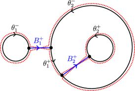
(a) When $\theta_{1}^{+}>0$.

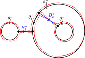
(b) When $\theta_{1}^{+}<0$.

Figure 22. A simple example with a crossing parameter $\theta_{1}^{+}$. The dotted curve is the element of the homotopy class of $\mathbf{c}_{i}$ constructed in §3 to express $\ell_{Y}(\mathbf{c}_{i})$.

In order to solve this issue, depending on the metric $Y$, we shall find a new representative of the homotopy class of a component ${\mathbf{c}}_{i}$ of $\mathbf{c}$, and introduce new positive variables $\tilde{\theta}_{q}$, such that the expression of $\ell_{Y}({\mathbf{c}}_{i})$ in those new variables now belongs to the desired class of functions $\mathcal{E}$. The idea is that, when a crossing variable is negative, we can rectify the problem by a basic move: if $\operatorname{Sign}(q)\operatorname{Sign}(\sigma q)=+1$ and $\theta_{q}<0$, the basic move consists in replacing $\overline{B}_{\sigma^{-1}q,q}\mathord{\mathchoice{\,\vbox{\hbox{\scalebox{0.5}{$\displaystyle\bullet$}}}\,}{\,\vbox{\hbox{\scalebox{0.5}{$\textstyle\bullet$}}}\,}{\,\vbox{\hbox{\scalebox{0.5}{$\scriptstyle\bullet$}}}\,}{\,\vbox{\hbox{\scalebox{0.5}{$\scriptscriptstyle\bullet$}}}\,}}\overline{\mathcal{I}}_{q}\mathord{\mathchoice{\,\vbox{\hbox{\scalebox{0.5}{$\displaystyle\bullet$}}}\,}{\,\vbox{\hbox{\scalebox{0.5}{$\textstyle\bullet$}}}\,}{\,\vbox{\hbox{\scalebox{0.5}{$\scriptstyle\bullet$}}}\,}{\,\vbox{\hbox{\scalebox{0.5}{$\scriptscriptstyle\bullet$}}}\,}}\overline{B}_{q,\sigma q}$ by the homotopic orthogeodesic $\overline{B}_{\sigma^{-1}q,\sigma q}$ from $\beta_{\sigma^{-1}q}$ to $\beta_{\sigma q}$. The segment $\overline{\mathcal{I}}_{q}$ is then said to be erased, and the variable $\theta_{q}$ is an erased variable. On Figure 23 we show a basic move in the case $\operatorname{Sign}(q)=\operatorname{Sign}(\sigma q)=+1$. We then perform these basic moves iteratively to get rid of all negative crossing variables.

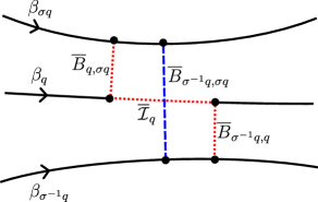
Figure 23. The basic move consists in replacing the dotted path with the dashed line in the homotopy class of $\mathbf{c}_{i}$.

We start this section by studying families of aligned geodesics in $\mathbb{H}^{2}$ and their orthogeodesics. We prove a key lemma called the staircase inequality in §7.2.2. We then construct the erasing procedure in §7.2.3; see Proposition 7.4. Once we lift our closed geodesic $\mathbf{c}_{i}$, loops $\beta$ and bars $B$ to the hyperbolic plane $\mathbb{H}^{2}$ as done in §4.2.2, we can apply Proposition 7.4 to them. This yields a partition of the Teichmüller space, as well as a new set of parameters $\tilde{\theta}_{q}$ on each element of this partition, as detailed in §7.3. The new length $\ell_{Y}(\mathbf{c}_{i})$ is expressed in these new parameters in §7.4. We then introduce a partition of unity adapted to this construction in §7.6.

For readers who decide to focus on the purely non-crossing case, it suffices to read §7.5-7.6.

7.2. Families of aligned geodesics and their orthogeodesics

Let us group together a few key observations about families of aligned geodesics and their orthogeodesics, which will be key to this section. In this whole subsection, we shall consider the following set-up. For an integer $M\geq 2$, $\gamma_{0},\ldots,\gamma_{M}$ are $M+1$ oriented geodesics in the hyperbolic plane. We assume that they are pairwise aligned, and that $\gamma_{i+1}$ is on the left of $\gamma_{i}$. We define $\overline{B}_{ij}$ to be the oriented orthogeodesics from $\gamma_{i}$ to $\gamma_{j}$, of length denoted by $L_{ij}>0$, and $z_{ij}\in\gamma_{j}$ (resp. $z_{ji}\in\gamma_{i}$) the endpoint (resp. origin) of $\overline{B}_{ij}$.

7.2.1. The $3$-geodesic lemma

First, we prove the following elementary observation.

Lemma 7.1.

Let $j\in\{1,\ldots,M-1\}$. Then,

(7.1) $$\vec{\mathrm{d}}(z_{j,j+1},z_{j-1,j+1})\geq 0\quad\Leftrightarrow\quad\vec{\mathrm{d}}(z_{j+1,j},z_{j-1,j})\geq 0\quad\Leftrightarrow\quad\vec{\mathrm{d}}(z_{j+1,j-1},z_{j,j-1})\geq 0$$

and, in terms of absolute distances,

(7.2) $$|\vec{\mathrm{d}}(z_{j+1,j},z_{j-1,j})|>|\vec{\mathrm{d}}(z_{j+1,j-1},z_{j,j-1})|+|\vec{\mathrm{d}}(z_{j,j+1},z_{j-1,j+1})|.$$

Proof.

These results stem from the elementary study of the polygon of consecutive vertices $z_{j-1,j+1}$, $z_{j,j+1}$, $z_{j+1,j}$, $z_{j-1,j}$, $z_{j,j-1}$, $z_{j+1,j-1}$ represented in Figure 24.

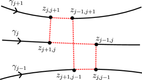
Figure 24. Illustration of the proof of Lemma 7.1.

Equation (7.1) is obtained by observing that there exists no hyperbolic hexagon with $5$ inner angles equal to $\pi/2$ and one equal to $3\pi/2$, and hence the polygon is a self-intersecting right-angled hexagon. Then, (7.2) is a direct consequence of the classic trigonometric formula for self-intersecting right-angled hexagons of consecutive side-lengths $(\ell_{i})_{1\leq i\leq 6}$ (see e.g. [5, Theorem 2.4.4]):

$$\cosh(\ell_{3})=\cosh(\ell_{1})\cosh(\ell_{5})+\cosh(\ell_{6})\sinh(\ell_{1})\sinh(\ell_{5})>\cosh(\ell_{1}+\ell_{5}).$$

∎

7.2.2. The staircase inequality

Let us now prove an inequality which we will refer to as the staircase inequality, illustrated in Figure 25.

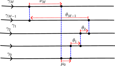
Figure 25. The geometric situation for the staircase inequality.

Lemma 7.2.

Let $M\geq 2$. We introduce the distances

$$\theta_{j}=\vec{\mathrm{d}}(z_{j-1,j},z_{j+1,j}),\quad\mu_{j}=\vec{\mathrm{d}}(z_{M,j},z_{j+1,j}),\quad\nu_{M}=\vec{\mathrm{d}}(z_{M-1,M},z_{0,M}).$$

Assume that $\theta_{j}\geq 0$ for $1\leq j\leq M-2$, that $\theta_{M-1}<0$, and that $\mu_{j}>0$ for $0\leq j\leq M-2$. Then,

(7.3) $$|\theta_{M-1}|>\sum_{j=1}^{M-2}\theta_{j}+\mu_{0}+\nu_{M}.$$

Remark 7.3.

The inequality (7.3) can also be written in the form

(7.4) $$-\sum_{j=1}^{M-1}\theta_{j}>\mu_{0}+\nu_{M}.$$

Proof.

We apply Lemma 7.1 to the geodesics $\gamma_{j-1}$, $\gamma_{j}$ and $\gamma_{M}$. We obtain that

(7.5) $$u_{j}:=\vec{\mathrm{d}}(z_{M,j},z_{j-1,j})>\vec{\mathrm{d}}(z_{M,j-1},z_{j,j-1})+\vec{\mathrm{d}}(z_{j,M},z_{j-1,M}),$$

all of these quantities being positive thanks to the hypothesis $\mu_{j-1}>0$ and (7.1).

For $2\leq j\leq M$, going along $\gamma_{j-1}$, we have the identity

$$\vec{\mathrm{d}}(z_{M,j-1},z_{j,j-1})=\vec{\mathrm{d}}(z_{M,j-1},z_{j-2,j-1})+\vec{\mathrm{d}}(z_{j-2,j-1},z_{j,j-1})=u_{j-1}+\theta_{j-1},$$

and for $j=1$, $\vec{\mathrm{d}}(z_{M,0},z_{1,0})=\mu_{0}$. As a consequence, (7.5) can be rewritten in terms of the sequence $(u_{j})_{j}$ as:

$$\begin{cases}u_{j}>u_{j-1}+\theta_{j-1}+\vec{\mathrm{d}}(z_{j,M},z_{j-1,M})&(j\geq 2)\\ u_{1}>\mu_{0}+\vec{\mathrm{d}}(z_{1,M},z_{0,M})&(j=1).\end{cases}$$

The result follows by induction, using that $u_{M-1}=|\theta_{M-1}|$ and $\nu_{M}=\sum_{j=1}^{M-1}\vec{\mathrm{d}}(z_{j,M},z_{j-1,M}).$ ∎

7.2.3. Erasing the negative crossings

We are now ready to prove the main result of this section, the contruction of the erasing procedure. We denote as $\vec{\theta}\in\mathbb{R}^{M-1}$ the vector $\theta_{j}=\vec{\mathrm{d}}(z_{j-1,j},z_{j+1,j})$ for all $1\leq j\leq M-1$, and $\vec{L}\in\mathbb{R}_{>0}^{M}$ the vector of components $L_{j,j+1}$, $0\leq j<M$. We note that the geometry of our family of aligned geodesics is entirely determined by the values of the parameters $\vec{L},\vec{\theta}$ (which belong in a subset of $\mathbb{R}_{>0}^{M}\times\mathbb{R}^{M-1}$).

Proposition 7.4.

Let $M\geq 2$ and $\vec{L}\in\mathbb{R}_{>0}^{M}$ be a fixed length-vector. There exists a partition $(P_{\xi})_{\xi\in\Xi_{M}}$ of $\mathbb{R}^{M-1}$ and a family $(I(\xi))_{\xi\in\Xi_{M}}$ of subsets

$$I(\xi)=\{0=\varphi_{\xi}(0)<\varphi_{\xi}(1)<\ldots<\varphi_{\xi}(K_{\xi}+1)=M\}$$

such that the following holds. Let $\xi\in\Xi_{M}$. For any $\vec{\theta}\in P_{\xi}$,

1. for any $1\leq j\leq K_{\xi}$, $\vec{\mathrm{d}}(z_{\varphi_{\xi}(j-1),\varphi_{\xi}(j)},z_{\varphi_{\xi}(j+1),\varphi_{\xi}(j)})\geq 0$;

2. for $0\leq j\leq K_{\xi}$, if we set

   $$\mu_{\varphi_{\xi}(j)}:=\vec{\mathrm{d}}(z_{\varphi_{\xi}(j+1),\varphi_{\xi}(j)},z_{\varphi_{\xi}(j)+1,\varphi_{\xi}(j)})$$

   $$\nu_{\varphi_{\xi}(j+1)}:=\vec{\mathrm{d}}(z_{\varphi_{\xi}(j+1)-1,\varphi_{\xi}(j+1)},z_{\varphi_{\xi}(j),\varphi_{\xi}(j+1)})$$

   then both of these distances are positive;

3. for $0\leq j\leq K_{\xi}$,

   (7.6) $$-\sum_{\varphi_{\xi}(j)<k<\varphi_{\xi}(j+1)}\theta_{k}\geq\mu_{\varphi_{\xi}(j)}+\nu_{\varphi_{\xi}(j+1)}.$$

Intuitively, this statement uses a combination of basic moves, together with the staircase inequality, to extract a path homotopic to the initial path, but with only positive turns. This is illustrated in Figure 26. Moving forward, we will use Proposition 7.4 to erase the variables $\theta_{k}$ with $k\notin I(\xi)$. This includes all of the negative $\theta_{k}$, but also the $\theta_{k}$ that are “not positive enough” to compensate for the existence of negative ones. Inequality 7.6 says that the sum of erased $\theta_{k}$ is negative, and gives a lower bound on its absolute value.

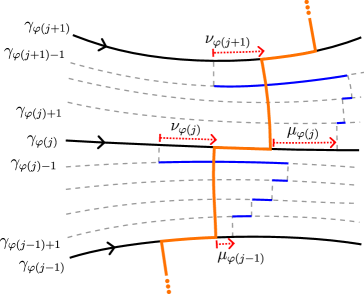
Figure 26. Illustration of the statement of Proposition 7.4.

Remark 7.5.

The partition is indexed by some set $\Xi_{M}$, the definition of which will be determined in the proof, but is of no particular interest. It is worth noting from the proof that the elements $P_{\xi}$ of the partition are products of intervals.

Remark 7.6.

We have fixed the lengths $\vec{L}$ because the whole discussion depends implicitly on the value of $\vec{L}$, although not apparent in the notation. The dependency on $\vec{L}$ shall not be relevant to our purposes.

Proof.

We shall prove the proposition by induction on the integer $M$, using a succession of basic moves. If $M=2$, the partition of $\mathbb{R}$ is $\mathbb{R}_{<0}\sqcup\mathbb{R}_{\geq 0}$. More precisely, the sets $I$ are as follows.

• If $\theta_{1}\geq 0$, there is nothing to be done, and we take $I=\{0,1,2\}$ (i.e. $K=M-1=1$ and $\varphi$ is the identity).

• If $\theta_{1}<0$, then we perform a basic move, that is, we take $I=\{0,2\}$. Inequality (7.2) then implies the claim that $|\theta_{1}|>\vec{\mathrm{d}}(z_{2,0},z_{1,0})+\vec{\mathrm{d}}(z_{1,2},z_{0,2})=\mu_{0}+\nu_{2}$.

Assume now that the construction has been achieved at the rank $M$, and extend it to the next rank $M+1$, i.e. to a family of aligned geodesics $\gamma_{0},\ldots,\gamma_{M+1}$. We apply the construction to the geodesics $\gamma_{0},\ldots,\gamma_{M}$ and obtain a partition $(P_{\xi})_{\xi\in\Xi_{M}}$ of $\mathbb{R}^{M-1}$ and a family of sets

$$I(\xi)=\{0=\varphi_{\xi}(0)<\varphi_{\xi}(1)<\ldots<\varphi_{\xi}(K_{\xi}+1)=M\}$$

satisfying the properties (a), (b), (c). Let us now construct a partition $(P_{\xi^{\prime}}^{\prime})_{\xi^{\prime}\in\Xi_{M+1}}$ of $\mathbb{R}^{M}$ and a family of sets $I^{\prime}(\xi^{\prime})$ (associated to a function $\varphi_{\xi^{\prime}}^{\prime}$ and an integer $K_{\xi^{\prime}}^{\prime}$) satisfying (a), (b), (c) at the rank $M+1$.

We shall partition

$$\mathbb{R}^{M}=\mathbb{R}^{M-1}\times\mathbb{R}=\bigsqcup_{\xi\in\Xi_{M}}(P_{\xi}\times\mathbb{R})$$

by partitionning each individual $P_{\xi}\times\mathbb{R}$. Let $\xi\in\Xi_{M}$ be fixed – to simplify notations, we drop the mention of $\xi$ in $\varphi_{\xi}$ and $K_{\xi}$. Let us cut the $\mathbb{R}$-component of $P_{\xi}\times\mathbb{R}$ (related to the value of $\theta_{M}$) depending on the relative positions of the points $z_{\varphi(K),M}$ and $z_{M+1,M}$ along $\gamma_{M}$.

• If the segment $[z_{\varphi(K),M},z_{M+1,M}]$ is positively oriented, there is nothing to be done, and we simply let $I^{\prime}=I(\xi)\cup\{M+1\}$ (in which case $K^{\prime}=K+1$).

• Otherwise, using (7.1), we observe that for any $k\in\{1,\ldots,K\}$,

  $$\vec{\mathrm{d}}(z_{M+1,\varphi(k)},z_{\varphi(k+1),\varphi(k)})\geq 0\quad\Rightarrow\quad\forall j\geq k,\quad\vec{\mathrm{d}}(z_{M+1,\varphi(j)},z_{\varphi(j-1),\varphi(j)})>0$$

  $$\vec{\mathrm{d}}(z_{\varphi(k-1),\varphi(k)},z_{M+1,\varphi(k)})\geq 0\quad\Rightarrow\quad\forall j\leq k,\quad\vec{\mathrm{d}}(z_{\varphi(j+1),\varphi(j)},z_{M+1,\varphi(j)})>0.$$

  We use this to establish the existence of a uniquely defined $K^{\prime}\in\{0,\ldots,K\}$, represented in Figure 27, such that the following two conditions hold:

  (7.7) $$\begin{split}\forall 0\leq j\leq K,\quad\big{(}\vec{\mathrm{d}}(z_{M+1,\varphi(j)},z_{\varphi(j+1),\varphi(j)})\geq 0&\quad\Leftrightarrow\quad j\geq K^{\prime}\big{)}\\ \forall 1\leq j\leq K,\quad\big{(}\vec{\mathrm{d}}(z_{\varphi(j-1),\varphi(j)},z_{M+1,\varphi(j)})>0&\quad\Leftrightarrow\quad j\leq K^{\prime}\big{)}.\end{split}$$

  

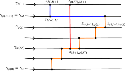
  Figure 27. In order to highlight the construction of the integer $K^{\prime}$, we have only represented the geodesics $\gamma_{\varphi(j)}$ for $0\leq j\leq K+1$ as well as $\gamma_{M+1}$, and the relevant orthogeodesics.

  We then let $I^{\prime}=\{\varphi(0),\ldots,\varphi(K^{\prime}),M+1\}$, a set associated to the integers $K^{\prime}$ and the function $\varphi^{\prime}$ which coincides with $\varphi$ for $j\leq K^{\prime}$ and is equal to $M+1$ at $K^{\prime}+1$.

Let us now construct the partition in more detail. We temporarily revert to notations depending on $\xi$ for clarity. For any $K^{\prime}\in\{0,\ldots,K_{\xi}+1\}$, we denote as $E_{K^{\prime}}$ the set of values of $\theta_{M}\in\mathbb{R}$ such that:

• $\vec{\mathrm{d}}(z_{\varphi_{\xi}(K_{\xi}),M},z_{M+1,M})\geq 0$ if $K^{\prime}=K_{\xi}+1$;

• the set of conditions (7.7) holds if $K^{\prime}$ is an integer in $\{0,\ldots,K_{\xi}\}$.

We can then write $\mathbb{R}=\bigsqcup_{K^{\prime}=0}^{K_{\xi}+1}E_{K^{\prime}}$ for each individual $\xi\in\Xi_{M}$. This yields the partition

$$\mathbb{R}^{M}=\bigsqcup_{\xi^{\prime}\in\Xi_{M+1}}P^{\prime}_{\xi^{\prime}},\quad\text{where}\quad\Xi_{M+1}=\{(\xi,K^{\prime})\,:\,\xi\in\Xi_{M},0\leq K^{\prime}\leq K_{\xi}+1\}$$

and $P^{\prime}_{\xi^{\prime}}:=P_{\xi}\times E_{K^{\prime}}$ for $\xi^{\prime}=(\xi,K^{\prime})\in\Xi_{M+1}$.

Our choice of $K^{\prime}$ straighforwardly implies that (a) and (b) are satisfied. The condition (c) is automatic in the case $K^{\prime}=K+1$, and is the last thing that we need to check when $K^{\prime}\leq K$.

By the induction hypothesis and the construction of $I^{\prime}$, we already know that (7.6) holds for $j=1,\ldots,K^{\prime}-1$, and we just need to check it for $j=K^{\prime}$. That is, we need to prove that

$$-\sum_{\varphi(K^{\prime})<k<M+1}\theta_{k}\geq\vec{\mathrm{d}}(z_{M+1,\varphi(K^{\prime})},z_{\varphi(K^{\prime})+1,\varphi(K^{\prime})})+\vec{\mathrm{d}}(z_{M,M+1},z_{\varphi(K^{\prime}),M+1}).$$

In order to do so, we write

(7.8) $$\sum_{\varphi(K^{\prime})<k<M+1}\theta_{k}=\sum_{j=K^{\prime}+1}^{K+1}\theta_{\varphi(j)}+\sum_{j=K^{\prime}}^{K}\sum_{\varphi(j)<k<\varphi(j+1)}\theta_{k}.$$

In order to bound the first term, we apply the staircase inequality, Lemma 7.2 (under the form (7.4)), to the geodesics $\gamma_{\varphi(j)}$ for $K^{\prime}\leq j\leq K$ and $\gamma_{M+1}$. The conditions (a) and (b) allow to verify the hypotheses. We obtain

(7.9) $$\begin{split}&-\sum_{j=K^{\prime}+1}^{K}\vec{\mathrm{d}}(z_{\varphi(j-1),\varphi(j)},z_{\varphi(j+1),\varphi(j)})-\vec{\mathrm{d}}(z_{\varphi(K),M},z_{M+1,M})\\ &>\vec{\mathrm{d}}(z_{M+1,\varphi(K^{\prime})},z_{\varphi(K^{\prime}+1),\varphi(K^{\prime})})+\vec{\mathrm{d}}(z_{M,M+1},z_{\varphi(K^{\prime}),M+1}).\end{split}$$

We then relate each of the terms on the left-hand-side to a $\theta_{\varphi(j)}$ by writing for $j\leq K$

$$\begin{split}\theta_{\varphi(j)}&=\vec{\mathrm{d}}(z_{\varphi(j)-1,\varphi(j)},z_{\varphi(j)+1,\varphi(j)})\\ &=\vec{\mathrm{d}}(z_{\varphi(j)-1,\varphi(j)},z_{\varphi(j-1),\varphi(j)})+\vec{\mathrm{d}}(z_{\varphi(j-1),\varphi(j)},z_{\varphi(j+1),\varphi(j)})+\vec{\mathrm{d}}(z_{\varphi(j+1),\varphi(j)},z_{\varphi(j)+1,\varphi(j)})\\ &=\nu_{\varphi(j)}+\vec{\mathrm{d}}(z_{\varphi(j-1),\varphi(j)},z_{\varphi(j+1),\varphi(j)})+\mu_{\varphi(j)}\end{split}$$

and similarly

$$\theta_{\varphi(K+1)}=\theta_{M}=\vec{\mathrm{d}}(z_{M-1,M},z_{M+1,M})=\nu_{\varphi(K+1)}+\vec{\mathrm{d}}(z_{\varphi(K),M},z_{M+1,M}).$$

Equation (7.9) then becomes

(7.10) $$\begin{split}&-\sum_{j=K^{\prime}+1}^{K+1}\theta_{\varphi(j)}+\sum_{j=K^{\prime}+1}^{K}\mu_{\varphi(j)}+\sum_{j=K^{\prime}}^{K}\nu_{\varphi(j+1)}\\ &>\vec{\mathrm{d}}(z_{M+1,\varphi(K^{\prime})},z_{\varphi(K^{\prime}+1),\varphi(K^{\prime})})+\vec{\mathrm{d}}(z_{M,M+1},z_{\varphi(K^{\prime}),M+1}).\end{split}$$

Now, to bound the second sum in (7.8), we apply the induction hypothesis to $K^{\prime}\leq j\leq K$, which yields:

(7.11) $$-\sum_{\varphi(j)<k<\varphi(j+1)}\theta_{k}>\mu_{\varphi(j)}+\nu_{\varphi(j+1)}.$$

Summing (7.10) with (7.11) for all $K^{\prime}\leq j\leq K$ allows to obtain, due to (7.8), that

$$-\sum_{\varphi(K^{\prime})<k<M+1}\theta_{k}>\vec{\mathrm{d}}(z_{M+1,\varphi(K^{\prime})},z_{\varphi(K^{\prime}+1),\varphi(K^{\prime})})+\vec{\mathrm{d}}(z_{M,M+1},z_{\varphi(K^{\prime}),M+1})+\mu_{\varphi(K^{\prime})}.$$

(we notice that all but one of the terms $\mu_{\varphi(j)}$ and $\nu_{\varphi(j+1)}$ vanish). The conclusion then follows, observing that

$$\vec{\mathrm{d}}(z_{M+1,\varphi(K^{\prime})},z_{\varphi(K^{\prime}+1),\varphi(K^{\prime})})+\mu_{\varphi(K^{\prime})}=\vec{\mathrm{d}}(z_{M+1,\varphi(K^{\prime})},z_{\varphi(K^{\prime})+1,\varphi(K^{\prime})}).$$

∎

Remark 7.7.

We can apply a similar construction to families of aligned geodesics ordered in the opposite order, i.e. such that $\gamma_{i+1}$ is now on the right of $\gamma_{i}$. Importantly, in this case, we do not reverse the direction of the hypotheses (b) (otherwise, the construction would be exactly the same and of no additional interest). See Figure 28.

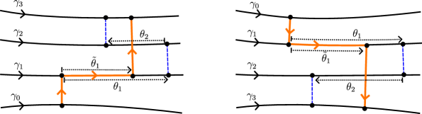
Figure 28. Two examples with $M=3$ and positive or negative crossings.

7.3. Crossing intervals and erasing of negative crossing parameters

In this section, we lift the geodesics $\beta$ to the hyperbolic plane, and apply Proposition 7.4 to erase all negative crossing variables. This yields newly defined positive variables $(\tilde{\theta}_{q})_{q\in I(\xi)}$. We will rely on the periodic re-indexation of $\Theta$ introduced in §2.5 as well as the lifting from §4.2.2.

The forthcoming discussion, in the case of purely non-crossing eights, is essentially empty.

7.3.1. Decomposition of $\Theta^{i}$ in crossing intervals

Let $i\in\{1,\ldots,\mathfrak{n}\}$. We decompose the set $\Theta^{i}\sim\mathbb{Z}_{n_{i}}$ according to the signs of its elements.

Notation 7.8.

We let $I_{1}^{+},\ldots,I_{p}^{+}\subseteq\Theta^{i}$ denote the connected components (maximal subintervals) of $\{q\in\Theta^{i},\operatorname{Sign}(q)=+\}$, and $I_{1}^{-},\ldots,I_{p}^{-}\subseteq\Theta^{i}$ the connected components of the complement. We call the intervals $I_{j}^{\delta}$ crossing intervals ($j=1,\ldots,p$, $\delta=\pm$). Actual crossings correspond to intervals $I_{j}^{\delta}$ of length $\geq 2$.

Remark 7.9.

If the function $\operatorname{Sign}$ is constant on $\Theta^{i}$, then $p=1$ (there is only one crossing interval), and we either have $I_{1}^{+}=\emptyset$ or $I_{1}^{-}=\emptyset$. In all other cases, due to the cyclicity of $\Theta^{i}\sim\mathbb{Z}_{n_{i}}$, the crossing intervals alternate in signs, and hence the number of positive and negative crossing intervals are equal.

This decomposition of $\Theta^{i}$ in crossing intervals yields the partition

$$\Theta^{i}=\bigsqcup_{j=1}^{p}\bigsqcup_{\delta=\pm}I_{j}^{\delta},$$

which allows us to identify

$$\mathbb{R}^{\Theta^{i}}\simeq\prod_{j=1}^{p}\prod_{\delta=\pm}\mathbb{R}^{I_{j}^{\delta}}.$$

Note that crossing intervals $I_{j}^{\delta}$ ($j\in\mathbb{Z}$) can also be defined as subsets of ${\mathbf{\Theta}}^{i}$, after pre-composing with the projection map $\mathbb{Z}\longrightarrow\mathbb{Z}_{n_{i}}$. In that case we have $I_{j+p}^{\delta}=I_{j}^{\delta}+n_{i}$, where $p$ is the number of positive crossing intervals (equivalently, of negative crossing intervals).

7.3.2. Application of the erasing procedure to one crossing interval

Let $j\in\{1,\ldots,p\}$ be an actual crossing. We write $I_{j}^{\delta}=\{q_{0}+1,\ldots,q_{0}+M\}$, where $M=\#I_{j}^{\delta}\geq 2$. By Lemma 4.1, we can apply Proposition 7.4 (and Remark 7.7 if $\delta=-$) to the family of $M+1$ aligned geodesics $\tilde{\beta}(q)$ with $q_{0}\leq q\leq q_{0}+M$, and obtain:

• a partition $(P_{\xi}^{o})_{\xi\in\Xi_{M}}$ of $\mathbb{R}^{\{q_{0}+1,\ldots,q_{0}+M-1\}}$;

• subsets $\{q_{0}=\varphi_{\xi}(0)<\varphi_{\xi}(1)<\ldots<\varphi_{\xi}(K_{\xi}+1)=q_{0}+M\}$ of $I_{j}^{\delta}\cup\{q_{0}\}$

satisfying the properties (a), (b), (c). We then define:

• $\Xi(I_{j}^{\delta})$ as a copy of $\Xi_{M}$;

• for $\xi=\xi_{j}^{\delta}\in\Xi(I_{j}^{\delta})$, $P_{\xi_{j}^{\delta}}=P_{\xi}^{o}\times\mathbb{R}$, so that $(P_{\xi_{j}^{\delta}})_{\xi_{j}^{\delta}\in\Xi(I_{j}^{\delta})}$ is a partition of $\mathbb{R}^{I_{j}^{\delta}}$;

• for $\xi\in\Xi(I_{j}^{\delta})$, $I_{j}^{\delta}(\xi):=\{\varphi_{\xi}(1)<\ldots<\varphi_{\xi}(K_{\xi}+1)\}$, which is a subinterval of $I_{j}^{\delta}$.

We extend this definition to the case where the crossing is not an actual crossing, by setting $(P_{\xi_{j}^{\delta}})_{\xi_{j}^{\delta}\in\Xi(I_{j}^{\delta})}$ to be the trivial partition $\mathbb{R}^{I_{j}^{\delta}}=\mathbb{R}$ indexed by a singleton set $\Xi(I_{j}^{\delta})$, and $I_{j}^{\delta}(\xi)=I_{j}^{\delta}$ in that case.

Remark 7.10.

Keep in mind that by construction, for any $\xi\in\Xi(I_{j}^{\delta})$, the interval $I_{j}^{\delta}(\xi)$ always contains the right endpoint $q_{0}+M$ of $I_{j}^{\delta}$, which is by definition a U-turn. The sets $P_{\xi_{j}^{\delta}}\subseteq\mathbb{R}^{I_{j}^{\delta}}$ all contain a full copy of $\mathbb{R}$ for the rightmost point of $I_{j}^{\delta}$, because the U-turn variables do not need to be controlled, by virtue of the Useful Remark, Remark 2.11. Indeed, it is automatic that the segments $[z_{q_{0}-1,q_{0}},z_{\varphi(1),q_{0}}]$ and $[z_{\varphi(K),q_{0}+M},z_{q_{0}+M+1,q_{0}+M}]$ are positively oriented.

Remark 7.11.

In the case described in Remark 7.9, the construction is slightly different at the last step of the induction. If $[z_{\varphi(K),n_{i}},z_{n_{i}+1,n_{i}}]$ is positively oriented, we proceed as normal, but if $[z_{\varphi(K),n_{i}},z_{n_{i}+1,n_{i}}]$ is negatively oriented, then we simply take $I(\xi)=\emptyset$.

Remark 7.12.

The construction is done in the universal cover. Since the covering group acts by isometries, if we replace $I$ by $I+n_{i}$, then the picture is translated by a hyperbolic isometry, namely the translation of axis $\tilde{\mathbf{c}}_{i}$ and of translation length $\ell({\mathbf{c}}_{i})$. This remark implies that the construction done in the universal cover projects down to ${\mathbf{S}}$, and that the subsets $I_{j}^{\delta}(\xi_{j}^{\delta})$ satisfy the invariance property $I_{j+p}^{\delta}(\xi_{j+p}^{\delta})=I_{j}^{\delta}(\xi_{j}^{\delta})+n_{i}$.

7.3.3. New representative of the homotopy class of $\mathbf{c}_{i}$

Let us show how our construction will be used to resolve the issue caused by the crossing interval $I_{j}^{\delta}$, raised in §6.5.

Notation 7.13.

Let $\xi\in\Xi(I_{j}^{\delta})$. For $q=\varphi_{\xi}(k)\in I_{j}^{\delta}(\xi)$, we consider the points

$$G_{q}:=z_{\varphi_{\xi}(k-1),\varphi_{\xi}(k)}\quad\text{and}\quad D_{q}:=z_{\varphi_{\xi}(k+1),\varphi_{\xi}(k)}.$$

We denote as $\mathcal{I}^{\prime}_{q}$ the segment $[G_{q},D_{q}]$ on $\tilde{\beta}(q)$.

By property (a), the segment $\tilde{\mathcal{I}}^{\prime}_{q}$ is positively oriented for every $q\in I_{j}^{\delta}(\xi)$. We observe that the portion $\tilde{p}_{q_{0}+1}\mathord{\mathchoice{\,\vbox{\hbox{\scalebox{0.5}{$\displaystyle\bullet$}}}\,}{\,\vbox{\hbox{\scalebox{0.5}{$\textstyle\bullet$}}}\,}{\,\vbox{\hbox{\scalebox{0.5}{$\scriptstyle\bullet$}}}\,}{\,\vbox{\hbox{\scalebox{0.5}{$\scriptscriptstyle\bullet$}}}\,}}\ldots\mathord{\mathchoice{\,\vbox{\hbox{\scalebox{0.5}{$\displaystyle\bullet$}}}\,}{\,\vbox{\hbox{\scalebox{0.5}{$\textstyle\bullet$}}}\,}{\,\vbox{\hbox{\scalebox{0.5}{$\scriptstyle\bullet$}}}\,}{\,\vbox{\hbox{\scalebox{0.5}{$\scriptscriptstyle\bullet$}}}\,}}\tilde{p}_{q_{0}+M}$ of the infinite path $\mathord{\mathchoice{\,\vbox{\hbox{\scalebox{0.5}{$\displaystyle\bullet$}}}\,}{\,\vbox{\hbox{\scalebox{0.5}{$\textstyle\bullet$}}}\,}{\,\vbox{\hbox{\scalebox{0.5}{$\scriptstyle\bullet$}}}\,}{\,\vbox{\hbox{\scalebox{0.5}{$\scriptscriptstyle\bullet$}}}\,}}_{q\in{\mathbf{\Theta}}^{i}}\;\tilde{p}(q)$ is homotopic, with endpoints gliding along $\tilde{\beta}(q_{0})$ and $\tilde{\beta}(q_{0}+M)$, to the path

(7.12) $$\tilde{B}_{q_{0},\varphi_{\xi}(1)}\mathord{\mathchoice{\,\vbox{\hbox{\scalebox{0.5}{$\displaystyle\bullet$}}}\,}{\,\vbox{\hbox{\scalebox{0.5}{$\textstyle\bullet$}}}\,}{\,\vbox{\hbox{\scalebox{0.5}{$\scriptstyle\bullet$}}}\,}{\,\vbox{\hbox{\scalebox{0.5}{$\scriptscriptstyle\bullet$}}}\,}}\mathcal{I}^{\prime}_{\varphi_{\xi}(1)}\mathord{\mathchoice{\,\vbox{\hbox{\scalebox{0.5}{$\displaystyle\bullet$}}}\,}{\,\vbox{\hbox{\scalebox{0.5}{$\textstyle\bullet$}}}\,}{\,\vbox{\hbox{\scalebox{0.5}{$\scriptstyle\bullet$}}}\,}{\,\vbox{\hbox{\scalebox{0.5}{$\scriptscriptstyle\bullet$}}}\,}}\ldots\mathord{\mathchoice{\,\vbox{\hbox{\scalebox{0.5}{$\displaystyle\bullet$}}}\,}{\,\vbox{\hbox{\scalebox{0.5}{$\textstyle\bullet$}}}\,}{\,\vbox{\hbox{\scalebox{0.5}{$\scriptstyle\bullet$}}}\,}{\,\vbox{\hbox{\scalebox{0.5}{$\scriptscriptstyle\bullet$}}}\,}}\tilde{B}_{\varphi_{\xi}(k-1),\varphi_{\xi}(k)}\mathord{\mathchoice{\,\vbox{\hbox{\scalebox{0.5}{$\displaystyle\bullet$}}}\,}{\,\vbox{\hbox{\scalebox{0.5}{$\textstyle\bullet$}}}\,}{\,\vbox{\hbox{\scalebox{0.5}{$\scriptstyle\bullet$}}}\,}{\,\vbox{\hbox{\scalebox{0.5}{$\scriptscriptstyle\bullet$}}}\,}}\mathcal{I}^{\prime}_{\varphi_{\xi}(k)}\mathord{\mathchoice{\,\vbox{\hbox{\scalebox{0.5}{$\displaystyle\bullet$}}}\,}{\,\vbox{\hbox{\scalebox{0.5}{$\textstyle\bullet$}}}\,}{\,\vbox{\hbox{\scalebox{0.5}{$\scriptstyle\bullet$}}}\,}{\,\vbox{\hbox{\scalebox{0.5}{$\scriptscriptstyle\bullet$}}}\,}}\tilde{B}_{\varphi_{\xi}(j),\varphi_{\xi}(j+1)}\mathord{\mathchoice{\,\vbox{\hbox{\scalebox{0.5}{$\displaystyle\bullet$}}}\,}{\,\vbox{\hbox{\scalebox{0.5}{$\textstyle\bullet$}}}\,}{\,\vbox{\hbox{\scalebox{0.5}{$\scriptstyle\bullet$}}}\,}{\,\vbox{\hbox{\scalebox{0.5}{$\scriptscriptstyle\bullet$}}}\,}}\ldots\mathord{\mathchoice{\,\vbox{\hbox{\scalebox{0.5}{$\displaystyle\bullet$}}}\,}{\,\vbox{\hbox{\scalebox{0.5}{$\textstyle\bullet$}}}\,}{\,\vbox{\hbox{\scalebox{0.5}{$\scriptstyle\bullet$}}}\,}{\,\vbox{\hbox{\scalebox{0.5}{$\scriptscriptstyle\bullet$}}}\,}}\mathcal{I}^{\prime}_{\varphi_{\xi}(K)}\mathord{\mathchoice{\,\vbox{\hbox{\scalebox{0.5}{$\displaystyle\bullet$}}}\,}{\,\vbox{\hbox{\scalebox{0.5}{$\textstyle\bullet$}}}\,}{\,\vbox{\hbox{\scalebox{0.5}{$\scriptstyle\bullet$}}}\,}{\,\vbox{\hbox{\scalebox{0.5}{$\scriptscriptstyle\bullet$}}}\,}}\tilde{B}_{\varphi_{\xi}(K),q_{0}+M}.$$

This is the path represented in Figure 27. We therefore see that Proposition 7.4 allows to replace our original representation of $\tilde{\mathbf{c}}_{i}$, where the segments $\tilde{\mathcal{I}}(q)$ could be oriented in any direction, to a new one where the segments $\mathcal{I}^{\prime}_{\varphi_{\xi}(k)}$ are positively oriented.

7.3.4. Erasing of all crossing intervals in $\Theta^{i}$

Let us now apply the erasing procedure simultanously to all crossing intervals in $\Theta^{i}$.

Notation 7.14.

We define for the component $\mathbf{c}_{i}$ the set

(7.13) $$\Xi^{i}:=\prod_{1\leq j\leq p}\prod_{\delta=\pm}\Xi(I_{j}^{\delta}).$$

We denote as $\xi^{i}=(\xi_{j}^{\delta})_{\begin{subarray}{c}1\leq j\leq p\\ \delta=\pm\end{subarray}}$ the elements of $\Xi^{i}$, and for such a $\xi^{i}$, we let

(7.14) $$P_{\xi^{i}}:=\prod_{j=1}^{p}\prod_{\delta=\pm}P_{\xi_{j}^{\delta}}\subseteq\prod_{j=1}^{p}\prod_{\delta=\pm}\mathbb{R}^{I_{j}^{\delta}}=\mathbb{R}^{\Theta^{i}}$$

and

(7.15) $$I(\xi^{i})=\bigsqcup_{j=1}^{p}\bigsqcup_{\delta=\pm}I_{j}^{\delta}(\xi_{j}^{\delta}),\quad\quad\tilde{I}(\xi^{i})=\bigsqcup_{j\in\mathbb{Z}}\bigsqcup_{\delta=\pm}I_{j}^{\delta}(\xi_{j}^{\delta}).$$

We denote $n_{\xi^{i}}=\#I(\xi^{i})$.

The collection $(P_{\xi^{i}})_{\xi^{i}\in\Xi^{i}}$ then forms a partition of $\mathbb{R}^{\Theta^{i}}$. The set $I(\xi^{i})$ is a subset of $\Theta^{i}$ while $\tilde{I}(\xi^{i})$ is the corresponding $n_{i}\mathbb{Z}$-periodic subset of ${\mathbf{\Theta}}^{i}$. Because $I_{j}^{\delta}(\xi_{j}^{\delta})$ always has the same right endpoint as $I_{j}^{\delta}$, $I(\xi^{i})$ contains all the U-turn variables in $\Theta^{i}$.

7.3.5. New variables $\tilde{\theta}_{q}$ and crossing inequality

For $\xi^{i}\in\Xi^{i}$, the sets $I(\xi^{i})$ and $\tilde{I}(\xi^{i})$ can be described by an increasing function $(\varphi_{k})_{k\in\mathbb{Z}}$ with values in $\mathbf{\Theta}^{i}$ such that $\varphi_{k+\#I(\xi^{i})}=\varphi_{k}+n_{i}$.

Notation 7.15.

Let $\xi^{i}\in\Xi^{i}$. For $q=\varphi_{k}\in I(\xi^{i})$, we denote as:

• $G_{q}:=z_{\varphi_{k-1},\varphi_{k}}$ and $D_{q}:=z_{\varphi_{k+1},\varphi_{k}}$;

• $\mathcal{I}^{\prime}_{q}$ the segment $[G_{q},D_{q}]$ on $\tilde{\beta}(q)$, and $\tilde{\theta}_{q}$ its length;

• $\tilde{L}_{q}=L_{\varphi_{k-1},\varphi_{k}}$ the length of the orthogeodesic $\tilde{B}_{\varphi_{k-1},\varphi_{k}}$.

By property (a), the segment $\mathcal{I}^{\prime}_{q}$ is always positively oriented and hence $\tilde{\theta}_{q}\geq 0$.

We can now adapt (7.12) and now simultaneous erase all crossing intervals. Indeed, the infinite concatenation $\mathord{\mathchoice{\,\vbox{\hbox{\scalebox{0.5}{$\displaystyle\bullet$}}}\,}{\,\vbox{\hbox{\scalebox{0.5}{$\textstyle\bullet$}}}\,}{\,\vbox{\hbox{\scalebox{0.5}{$\scriptstyle\bullet$}}}\,}{\,\vbox{\hbox{\scalebox{0.5}{$\scriptscriptstyle\bullet$}}}\,}}_{k\in\mathbb{Z}}\big{(}\tilde{B}_{\varphi_{k-1},\varphi_{k}}\mathord{\mathchoice{\,\vbox{\hbox{\scalebox{0.5}{$\displaystyle\bullet$}}}\,}{\,\vbox{\hbox{\scalebox{0.5}{$\textstyle\bullet$}}}\,}{\,\vbox{\hbox{\scalebox{0.5}{$\scriptstyle\bullet$}}}\,}{\,\vbox{\hbox{\scalebox{0.5}{$\scriptscriptstyle\bullet$}}}\,}}\mathcal{I}^{\prime}_{\varphi_{k}}\big{)}$ gives an infinite curve in the hyperbolic plane, which projects down to a curve homotopic to the lift $\tilde{\mathbf{c}}_{i}$ of $\mathbf{c}_{i}$ to $\mathbb{H}$. The fact that the new path does no longer go along $\tilde{\mathcal{I}}(q)$ for $q\in\tilde{I}(\xi^{i})$ motivates the following terminology.

Definition 7.16.

The variables $\theta_{q}$ for $q\in\Theta^{i}\setminus\tilde{I}(\xi^{i})$ are said to be erased.

We can then restate the property (c) from Proposition 7.4 in the following equivalent way.

Lemma 7.17.

For any component $i$,

(7.16) $$\sum_{q\in\Theta^{i}}\theta_{q}<\sum_{q\in I(\xi^{i})}\tilde{\theta}_{q}.$$

Proof.

We simply notice that property (c) states that

(7.17) $$\sum_{q\in\Theta^{i}\setminus I(\xi^{i})}\theta_{q}<-\sum_{k=1}^{\#I(\xi^{i})}(\nu_{\varphi_{k+1}}+\mu_{\varphi_{k}})$$

with the notation $\mu,\nu$ from Proposition 7.4, and observe that by definition,

(7.18) $$\nu_{\varphi_{k}}+\tilde{\theta}_{\varphi_{k}}+\mu_{\varphi_{k}}=\theta_{\varphi_{k}}.$$

∎

Remark 7.18.

In the case described in Remarks 7.9 and 7.11, when the sign function is constant on $\Theta^{i}$, if $\xi$ is such that $I(\xi)=\emptyset$, then (7.16) means that

$$\sum_{q\in\Theta^{i}}\theta_{q}<0.$$

In this case it is sufficient to consider the geodesic representative of ${\mathbf{c}}_{i}$, and we won’t need to express the length $\ell_{Y}({\mathbf{c}}_{i})$ in coordinates.

7.3.6. Product over all components $\mathbf{c}_{i}$

Let us now group our constructions for the different components $\mathbf{c}_{1},\ldots,\mathbf{c}_{\mathfrak{n}}$ of the multiloop $\mathbf{c}$. In order to do so, we let $\Xi:=\prod_{i=1}^{\mathfrak{n}}\Xi^{i}$. We shall consider the cartesian product of the partitions $P_{\xi^{i}}$, that is, for $\xi=(\xi^{1},\ldots,\xi^{\mathfrak{n}})\in\Xi$, we let

(7.19) $$P_{\xi}=\prod_{i=1}^{\mathfrak{n}}P_{\xi^{i}}\quad\text{and}\quad I(\xi)=\bigsqcup_{i=1}^{\mathfrak{n}}I(\xi^{i})\subseteq\Theta.$$

The sets $(P_{\xi})_{\xi\in\Xi}$ then form a partition of $\prod_{i=1}^{\mathfrak{n}}\mathbb{R}^{\Theta^{i}}=\mathbb{R}^{\Theta}$. Each $P_{\xi}$ is a product of intervals.

We shall say that the variables $\theta_{q}$ for $q\not\in I(\xi)$ are erased. The set $I(\xi)$ contains all U-turn variables. As a consequence, in the purely non-crossing case, we have $I(\xi)=\Theta$ for all $\xi$, and all the previous discussion is empty.

7.4. New expression for the length

The erasing procedure immediately yields a new expression for $\ell_{Y}({\mathbf{c}})$, true for $\vec{\theta}\in P_{\xi}$, which replaces (4.12).

Proposition 7.19.

Let $\xi\in\Xi$. As soon as $\vec{\theta}\in P_{\xi}$, we have

(7.20) $$\ell_{Y}({\mathbf{c}})=\sum_{i=1}^{\mathfrak{n}}M_{n_{\xi^{i}}}((\epsilon\tilde{L}_{q})_{q\in I(\xi^{i})},(\tilde{\theta}_{q})_{q\in I(\xi^{i})})$$

where $n_{\xi^{i}}=\#I(\xi^{i})$, $\epsilon\tilde{L}_{q}:=\operatorname{Sign}(q)\tilde{L}_{q}$ and $M_{n}$ is defined in (4.10).

Proof.

For each $1\leq i\leq\mathfrak{n}$, we apply Proposition 4.6 to the representative $\mathord{\mathchoice{\,\vbox{\hbox{\scalebox{0.5}{$\displaystyle\bullet$}}}\,}{\,\vbox{\hbox{\scalebox{0.5}{$\textstyle\bullet$}}}\,}{\,\vbox{\hbox{\scalebox{0.5}{$\scriptstyle\bullet$}}}\,}{\,\vbox{\hbox{\scalebox{0.5}{$\scriptscriptstyle\bullet$}}}\,}}_{k\in\mathbb{Z}}\big{(}\tilde{B}_{\varphi_{k-1},\varphi_{k}}\mathord{\mathchoice{\,\vbox{\hbox{\scalebox{0.5}{$\displaystyle\bullet$}}}\,}{\,\vbox{\hbox{\scalebox{0.5}{$\textstyle\bullet$}}}\,}{\,\vbox{\hbox{\scalebox{0.5}{$\scriptstyle\bullet$}}}\,}{\,\vbox{\hbox{\scalebox{0.5}{$\scriptscriptstyle\bullet$}}}\,}}\mathcal{I}^{\prime}_{\varphi_{k}}\big{)}$ of the homotopy class of $\tilde{\mathbf{c}}_{i}$ on the subset $P_{\xi^{i}}$ of $\mathbb{R}^{\Theta^{i}}$. ∎

Note that, as long as $\vec{\theta}\in P_{\xi}$, each variable $\tilde{\theta}_{q}$ with $q\in I(\xi)$ is positive. As a consequence, this new formula solves the first issue raised in §6.5.

When using formula (7.20) later, we shall consider all the variables $\theta_{q}$ with $q\not\in I(\xi)$ as additional neutral parameters. The following observation will then be useful.

Lemma 7.20.

Let $\xi\in\Xi$. On the set $P_{\xi}$, for any $q\in I(\xi)$,

(7.21) $$\tilde{L}_{q}=\mathrm{fn}((\theta_{q^{\prime}})_{q^{\prime}\not\in I(\xi)},\vec{L})\quad\text{and}\quad\tilde{\theta}_{q}=\theta_{q}+\mathrm{fn}((\theta_{q^{\prime}})_{q^{\prime}\not\in I(\xi)},\vec{L}).$$

Proof.

Let $\xi\in\Xi$. For $1\leq i\leq\mathfrak{n}$, let us represent $\xi^{i}\in\Xi^{i}$ by a function $(\varphi_{k})_{k\in\mathbb{Z}}$. For $q\in I(\xi^{i})$, the length $\tilde{L}_{q}$ is the length of the orthogeodesic from $\tilde{\beta}(\varphi_{k-1})$ to $\tilde{\beta}(\varphi_{k})$, and therefore can be expressed as a function of $\vec{L}$ and the $\theta_{q^{\prime}}$ with $q^{\prime}\in\Theta^{i}$ such that $\varphi_{k-1}<q^{\prime}<\varphi_{k}$. This implies that $q^{\prime}\notin I(\xi)$, which was our claim.

Similarly, the quantities $\nu_{\varphi_{k}},\mu_{\varphi_{k}}$ can be expressed solely in terms of the $\theta_{q^{\prime}}$ with $q^{\prime}\not\in I(\xi)$. However, we have seen in (7.18) that $\theta_{\varphi_{k}}=\nu_{\varphi_{k}}+\tilde{\theta}_{\varphi_{k}}+\mu_{\varphi_{k}}$, which allows us to conclude. ∎

As a consequence, if we fix $(\theta_{q})_{q\not\in I(\xi^{i})}$ as well as $\vec{L}$, and view the expression (7.20) as a function of $(\tilde{\theta}_{q})_{q\in I(\xi^{i})}$, then Proposition 6.24 holds for this new length function.

Remark 7.21.

An intuition as to why the variables $\theta_{q}$ taking negative values yield additional neutral parameters can be found by examining Figure 22. Recall that we have motivated in §5.3 the fact that the lengths $\vec{L}$ are neutral parameters by observing that, when we describe the path $\mathbf{c}_{i}$ as the concatenation $\mathbf{c}_{i}^{\mathrm{op}}=\mathord{\mathchoice{\,\vbox{\hbox{\scalebox{0.5}{$\displaystyle\bullet$}}}\,}{\,\vbox{\hbox{\scalebox{0.5}{$\textstyle\bullet$}}}\,}{\,\vbox{\hbox{\scalebox{0.5}{$\scriptstyle\bullet$}}}\,}{\,\vbox{\hbox{\scalebox{0.5}{$\scriptscriptstyle\bullet$}}}\,}}_{q\in{{\Theta}}^{i}}\;p(q)$, each bar is visited twice, which mean that there is a factor of $2$ in front of each $L_{j}$ in our comparison estimates.

We see in the example of Figure 22 that, when $\theta_{1}^{+}<0$, the portion $\mathcal{I}_{1}^{+}$ is visited three times by the path $\mathbf{c}_{i}^{\mathrm{op}}$, instead of once when $\theta_{1}^{+}\geq 0$. This means that we do not need to apply the operator $\mathcal{L}$ to cancel exponential growth related to the parameter $\theta_{1}^{+}$, or, in other words, that it is a neutral parameter.

7.5. The purely non-crossing case

The reader only interested in the purely non-crossing case can read the rest of the paper, considering that $\Xi$ is a set with one element denoted $\xi=(\xi^{1},\ldots,\xi^{\mathfrak{n}})$, and that in what follows we let $I(\xi)=\Theta$, $I(\xi^{i})=\Theta^{i}$ for $i\in\{1,\ldots,\mathfrak{n}\}$. In this case we have $\tilde{\theta}_{q}=\theta_{q}$ for all $q\in\Theta$, as well as $\mathcal{I}^{\prime}_{q}=\overline{\mathcal{I}}_{q}=[G_{q},D_{q}]$.

7.6. A partition of unity on Teichmüller space

We recall that the space of interest in this article is the Teichmüller space $\mathcal{T}_{g_{\mathbf{S}},n_{\mathbf{S}}}^{\ast}$, which we have equipped with a new set of coordinates $(\vec{L},\vec{\theta})\in\mathbb{R}_{>0}^{r}\times\mathbb{R}^{\Theta}$. We have introduced a partition $\mathbb{R}^{\Theta}=\bigsqcup_{\xi\in\Xi}P_{\xi}$ that we wish to use on the parameter $\vec{\theta}$. Because our methods require some smoothness, it will be more convenient to partition the values of $\vec{\theta}$ using a partition of unity, which we shall now construct. Note that the entire discussion above is dependent on the length vector $\vec{L}$, although this has not been made explicit in the notation.

Notation 7.22.

Let $\chi_{\mathcal{C},0}$ and $\chi_{\mathcal{C},\infty}$ denote two smooth functions on $\mathbb{R}_{\geq 0}$ such that:

• $\chi_{\mathcal{C},0}+\chi_{\mathcal{C},\infty}\equiv 1$;

• $\chi_{\mathcal{C},0}$ is supported in $[0,2\log 2]$ and identically equal to $1$ on $[0,\log 2]$.

Definition 7.23.

For $\xi\in\Xi$ and $\mathcal{Q}\subseteq I(\xi)$, we define a cut-off function on Teichmüller space,

(7.22) $$\Psi_{\xi,\mathcal{Q}}(\vec{L},\vec{\theta})={\mathchoice{1\mskip-4.0mu{\rm{l}}}{1\mskip-4.0mu{\rm{l}}}{1\mskip-4.5mu{\rm{l}}}{1\mskip-5.0mu{\rm{l}}}}_{P_{\xi}}(\vec{L},\vec{\theta})\prod_{q\in\mathcal{Q}}\chi_{\mathcal{C},\infty}(\tilde{\theta}_{q})\prod_{q\not\in\mathcal{Q}}\chi_{\mathcal{C},0}(\tilde{\theta}_{q}).$$

By construction,

$$\sum_{\begin{subarray}{c}\xi\in\Xi\\ \mathcal{Q}\subseteq I(\xi)\end{subarray}}\Psi_{\xi,\mathcal{Q}}\equiv 1.$$

As announced in §7.4, we associate to each partition element some additional neutral variables.

Notation 7.24 (Neutral variables associated with $(\xi,\mathcal{Q})$).

For $\xi\in\Xi$ and $\mathcal{Q}\subseteq I(\xi)$, we let

(7.23) $$\Theta_{\mathrm{nt}}(\xi,\mathcal{Q})=\Theta\setminus\mathcal{Q}.$$

Note that, on the support of the cut-off function $\Psi_{\xi,\mathcal{Q}}$, the variables $(\tilde{\theta}_{q})_{q\in\Theta\setminus\mathcal{Q}}$ stay in $[0,2\log 2]$, so that we do not need to gain exponential decay in those variables. They can therefore be considered to be neutral variables.

8. The lengths of boundary curves

8.1. Objective and plan of the section

Recall that, in Proposition 4.11, we have obtained expressions for the lengths of the pair of pants decomposition $(\Gamma_{\lambda})_{\lambda\in\Lambda}$ in our new coordinates $(\vec{L},\vec{\theta})$ on the Teichmüller space $\mathcal{T}_{g_{\mathbf{S}},n_{\mathbf{S}}}^{*}$. This new expression reads $\ell_{Y}(\Gamma_{\lambda})=Q_{m}(\vec{L}^{\lambda},\vec{\tau}^{\lambda})$, where $\vec{L}^{\lambda}=(L^{\lambda}_{1},\ldots,L^{\lambda}_{m})$ and $\vec{\tau}^{\lambda}=(\tau^{\lambda}_{1},\ldots,\tau^{\lambda}_{m})$ are the parameters described in §4.4.2, $m=m(\lambda)$, and the functions $F_{m}$, $Q_{m}$ are defined in (4.20) by

(8.1) $$F_{m}(\vec{L},\vec{\tau})=\frac{\cosh(\frac{1}{2}Q_{m}(\vec{L},\vec{\tau}))}{\exp(\frac{1}{2}\sum_{j=1}^{m}\tau_{j})}=\frac{1}{2}\sum_{\alpha\in\{0,1\}^{m}}(-1)^{|\alpha|}\operatorname{hyp}_{-\partial\alpha}\left(\frac{\vec{L}}{2}\right)e^{-\alpha\cdot\vec{\tau}}$$

with $(\partial\alpha)_{j}=1$ if $\alpha_{j}=\alpha_{j-1}$ and $-1$ if $\alpha_{j}\not=\alpha_{j-1}$.

The aim of this section is to study the function $F_{m}$, and in particular its logarithmic derivatives, which will appear when we apply our key argument to the integral (5.13). The formula (8.1) is problematic because of its alternating signs: it is not clear which terms dominate the sum, nor is it that the formula gives a positive function. In fact, the domain $\mathfrak{D}$ of $(\vec{L},\vec{\theta})$ is precisely defined by the fact that the formula giving $\cosh(\ell_{Y}(\Gamma_{\lambda})/2)$ is greater than $1$ for all $\lambda\in\Lambda$, as seen in Proposition 3.21.

We work around this problem introducing a favorable region, i.e. a region of $\mathfrak{D}$ on which $F_{m}$ is well-approximated by its term with $\alpha=(0,\ldots,0)$, equal to $\prod_{j=1}^{m}\sinh(L_{j}/2)$. This domain is defined in terms of the heights of cells introduced in §8.4.1. We provide estimates on the derivatives of $F_{m}$ true inside the favorable region in Proposition 8.17. Outside the favorable region, the height of one (or several) cells must be bounded – we neutralize such cells. The neutralization procedure is to low-height cells what the erasing procedure was to negative $\theta$ parameters in §7. The description of the neutralization procedure while dealing simultanously with all of the boundary components $(\Gamma_{\lambda})_{\lambda\in\Lambda}$ requires some technical considerations, addressed in §8.5. In §8.6, we finally obtain a partition of unity of the Teichmüller space so that we understand the length of $\Gamma_{\lambda}$ and its derivatives on every piece of the partition.

8.2. Polygonal curves, neutralization, derivation

In §4.4, we have used a key observation on the structure of the curves $\Gamma_{\lambda}$ to compute their lengths: the fact that they can be viewed as a succession of perpendicular geodesic segments of alternating lengths $L_{j}^{\lambda},\tau_{j}^{\lambda}$, turning the same direction each time (see Figure 20). We shall introduce a notion of polygonal curve, which encapsulates this key property of $\Gamma_{\lambda}$. Let us first provide this definition without reference to a hyperbolic metric. Subsequently in §8.3, a hyperbolic metric will be given, and we will work with preferred “geodesic representatives”.

8.2.1. Definition of polygonal curves

In the following, we fix a base surface $\mathbf{S}$ and an oriented multi-curve $\beta$ on $\mathbf{S}$.

Definition 8.1.

A polygonal curve $\Gamma$ (on the surface ${\mathbf{S}}$ and based on $\beta$) is an oriented closed path without self-intersections, formed by a cyclic sequence $(J_{j},K_{j})_{j\in\mathbb{Z}_{m}}$ of oriented segments where, for all $j\in\mathbb{Z}_{m}$,

• $J_{j}$ meets the multi-curve $\beta$ at its endpoints and not in its interior, and is homotopically non-trivial with gliding endpoints along $\beta$;

• $K_{j}$ is a subsegment of $\beta$, possibly with reversed orientation;

• $J_{j}$ arrives at $K_{j}$ on the right at the point $t(J_{j})=o(K_{j})$, and $K_{j}$ arrives at $J_{j+1}$ on the right at the point $t(K_{j})=o(J_{j+1})$.

Note that the multi-curve $\beta$ is essential to this definition. The segments $J_{j}$ and $K_{j}$ play different roles and will therefore be named differently.

Definition 8.2.

The segments $K_{j}$ are called the cells of the polygonal curve $\Gamma$, and the $J_{j}$ its bridges. We denote $\operatorname{Cell}(\Gamma)=\{K_{j},j\in\mathbb{Z}_{m}\}$ and $\operatorname{Br}(\Gamma)=\{{J}_{j},j\in\mathbb{Z}_{m}\}$.

For a cell $K=K_{j}\in\operatorname{Cell}(\Gamma)$, the bridges adjacent to $K$ refer to the bridges $J_{j}$ and $J_{j+1}$. We respectively call these bridges the bridge arriving on $K$ and the bridge coming out of $K$.

Notation 8.3.

We call $m$ the combinatorial length of $\Gamma$, denoted $|\Gamma|$.

By convention, for $m=0$, a polygonal curve of combinatorial length $0$ is a simple curve that does not intersect the family $\beta$ (but may be homotopic to a component of $\beta$). In particular, polygonal curves of combinatorial length $0$ do not have any cells.

Example 8.4.

We have seen in §4.4.2 that each of the curves $(\Gamma_{\lambda})_{\lambda\in\Lambda}$ in the pair of pants decomposition defined in §3.2 is a polygonal curve based on $\beta$, where:

• the bridges $J_{j}$ are among the bars $B_{q}$;

• the cells $K_{j}$ are among the segments $\mathcal{K}_{qq^{\prime}}$ defined in §4.3.

The family $(\Gamma_{\lambda})_{\lambda\in\Lambda}$ will be the main example to which the whole discussion applies. For $\lambda\in\Lambda_{\mathrm{BC}}$, we can even say that the corresponding cells are among the segments $(\mathcal{K}_{q})_{q\in\Theta}$.

Note that the components $(\beta_{\lambda})_{\lambda\in\Lambda^{\beta}}$ are polygonal curves of combinatorial length $0$.

8.2.2. Neutralizing a cell

Let $\Gamma=(J_{j},K_{j})_{j\in\mathbb{Z}_{m}}$ be a polygonal curve on $\mathbf{S}$ of combinatorial length $m\geq 2$. Let $j\in\mathbb{Z}_{m}$. We may construct a new polygonal curve $\Gamma^{\prime}$ by replacing the sequence $(J_{j},K_{j},J_{j+1})$ in $\Gamma$ by one single bridge $\tilde{J}_{j}:=J_{j}\mathord{\mathchoice{\,\vbox{\hbox{\scalebox{0.5}{$\displaystyle\bullet$}}}\,}{\,\vbox{\hbox{\scalebox{0.5}{$\textstyle\bullet$}}}\,}{\,\vbox{\hbox{\scalebox{0.5}{$\scriptstyle\bullet$}}}\,}{\,\vbox{\hbox{\scalebox{0.5}{$\scriptscriptstyle\bullet$}}}\,}}K_{j}\mathord{\mathchoice{\,\vbox{\hbox{\scalebox{0.5}{$\displaystyle\bullet$}}}\,}{\,\vbox{\hbox{\scalebox{0.5}{$\textstyle\bullet$}}}\,}{\,\vbox{\hbox{\scalebox{0.5}{$\scriptstyle\bullet$}}}\,}{\,\vbox{\hbox{\scalebox{0.5}{$\scriptscriptstyle\bullet$}}}\,}}J_{j+1}$ (or a smoothened version thereof). This operation is represented in Figure 29(a). We observe that the derived polygonal curve $\Gamma^{\prime}$ we obtain is homotopic to $\Gamma$ and that its combinatorial length is $m-1$.

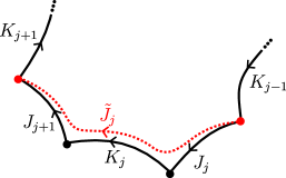
(a) One cell.

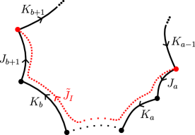
(b) Several cells.

Figure 29. Neutralization of one or several cells.

Definition 8.5.

The polygonal curve $\Gamma^{\prime}$ is said to be derived from $\Gamma$ by neutralizing the cell $K_{j}$. We call $\tilde{J}_{j}$ the roof over $K_{j}$. We denote $\tilde{K}_{j-1}:={K}_{j-1}$, $\tilde{K}_{j+1}:={K}_{j+1}$ the new cells of $\Gamma^{\prime}$.

The motivation for the name “new cells” will become apparent when we take geodesic representatives. The new polygonal curve $\Gamma^{\prime}$ satisfies

• $\operatorname{Br}(\Gamma^{\prime})=\{\tilde{J}_{j}\}\cup(\operatorname{Br}(\Gamma)\setminus\{J_{j},J_{j+1}\})$;

• $\operatorname{Cell}(\Gamma^{\prime})=\{\tilde{K}_{j-1},\tilde{K}_{j+1}\}\cup(\operatorname{Cell}(\Gamma)\setminus\{K_{j-1},K_{j},K_{j+1}\})$.

If now $\Gamma$ is a polygonal curve of combinatorial length $1$, we define $\tilde{J}_{1}$ as the simple closed curve $J_{1}\mathord{\mathchoice{\,\vbox{\hbox{\scalebox{0.5}{$\displaystyle\bullet$}}}\,}{\,\vbox{\hbox{\scalebox{0.5}{$\textstyle\bullet$}}}\,}{\,\vbox{\hbox{\scalebox{0.5}{$\scriptstyle\bullet$}}}\,}{\,\vbox{\hbox{\scalebox{0.5}{$\scriptscriptstyle\bullet$}}}\,}}K_{1}$ (or a smoothened verson thereof). Then $\Gamma^{\prime}=\tilde{J}_{1}$ is a polygonal curve of combinatorial length $0$ homotopic to $\Gamma$.

8.2.3. Simultaneous neutralization of several cells.

We now consider an interval $I=\{a,\ldots,b\}$ of $\mathbb{Z}_{m}$ of length $1\leq\#I<m$. Let us define $\tilde{J}_{I}:=J_{a}\mathord{\mathchoice{\,\vbox{\hbox{\scalebox{0.5}{$\displaystyle\bullet$}}}\,}{\,\vbox{\hbox{\scalebox{0.5}{$\textstyle\bullet$}}}\,}{\,\vbox{\hbox{\scalebox{0.5}{$\scriptstyle\bullet$}}}\,}{\,\vbox{\hbox{\scalebox{0.5}{$\scriptscriptstyle\bullet$}}}\,}}K_{a}\mathord{\mathchoice{\,\vbox{\hbox{\scalebox{0.5}{$\displaystyle\bullet$}}}\,}{\,\vbox{\hbox{\scalebox{0.5}{$\textstyle\bullet$}}}\,}{\,\vbox{\hbox{\scalebox{0.5}{$\scriptstyle\bullet$}}}\,}{\,\vbox{\hbox{\scalebox{0.5}{$\scriptscriptstyle\bullet$}}}\,}}\ldots\mathord{\mathchoice{\,\vbox{\hbox{\scalebox{0.5}{$\displaystyle\bullet$}}}\,}{\,\vbox{\hbox{\scalebox{0.5}{$\textstyle\bullet$}}}\,}{\,\vbox{\hbox{\scalebox{0.5}{$\scriptstyle\bullet$}}}\,}{\,\vbox{\hbox{\scalebox{0.5}{$\scriptscriptstyle\bullet$}}}\,}}K_{b}\mathord{\mathchoice{\,\vbox{\hbox{\scalebox{0.5}{$\displaystyle\bullet$}}}\,}{\,\vbox{\hbox{\scalebox{0.5}{$\textstyle\bullet$}}}\,}{\,\vbox{\hbox{\scalebox{0.5}{$\scriptstyle\bullet$}}}\,}{\,\vbox{\hbox{\scalebox{0.5}{$\scriptscriptstyle\bullet$}}}\,}}J_{b+1}$ (or a smoothened version thereof) and call $\tilde{J}_{I}$ the roof over $(K_{j})_{j\in I}$. A new polygonal curve $\Gamma^{\prime}$ may be obtained by replacing the sequence $(J_{a},K_{a},\ldots,K_{b},J_{b+1})$ by $\tilde{J}_{I}$, as represented in Figure 29(b). We then say that $\Gamma^{\prime}$ is derived from $\Gamma$ by neutralizing simultaneously all the $(K_{j})_{j\in I}$.

We denote $\tilde{K}_{a-1}:={K}_{a-1}$, $\tilde{K}_{b+1}:={K}_{b+1}$ and call them new cells of $\Gamma^{\prime}$. The new polygonal curve $\Gamma^{\prime}$ then satisfies:

• $\operatorname{Br}(\Gamma^{\prime})=\{\tilde{J}_{I}\}\cup(\operatorname{Br}(\Gamma)\setminus\{J_{a},J_{a+1},\ldots,J_{b+1}\})$;

• $\operatorname{Cell}(\Gamma^{\prime})=\{\tilde{K}_{a-1},\tilde{K}_{b+1}\}\cup(\operatorname{Cell}(\Gamma)\setminus\{K_{a-1},K_{a},\ldots,K_{b+1}\})$.

We extend these definitions to the case $I=\mathbb{Z}_{m}$, now taking $\Gamma^{\prime}$ to be a simple curve freely homotopic to the concatenation $J_{1}\mathord{\mathchoice{\,\vbox{\hbox{\scalebox{0.5}{$\displaystyle\bullet$}}}\,}{\,\vbox{\hbox{\scalebox{0.5}{$\textstyle\bullet$}}}\,}{\,\vbox{\hbox{\scalebox{0.5}{$\scriptstyle\bullet$}}}\,}{\,\vbox{\hbox{\scalebox{0.5}{$\scriptscriptstyle\bullet$}}}\,}}K_{1}\mathord{\mathchoice{\,\vbox{\hbox{\scalebox{0.5}{$\displaystyle\bullet$}}}\,}{\,\vbox{\hbox{\scalebox{0.5}{$\textstyle\bullet$}}}\,}{\,\vbox{\hbox{\scalebox{0.5}{$\scriptstyle\bullet$}}}\,}{\,\vbox{\hbox{\scalebox{0.5}{$\scriptscriptstyle\bullet$}}}\,}}\ldots\mathord{\mathchoice{\,\vbox{\hbox{\scalebox{0.5}{$\displaystyle\bullet$}}}\,}{\,\vbox{\hbox{\scalebox{0.5}{$\textstyle\bullet$}}}\,}{\,\vbox{\hbox{\scalebox{0.5}{$\scriptstyle\bullet$}}}\,}{\,\vbox{\hbox{\scalebox{0.5}{$\scriptscriptstyle\bullet$}}}\,}}J_{m}\mathord{\mathchoice{\,\vbox{\hbox{\scalebox{0.5}{$\displaystyle\bullet$}}}\,}{\,\vbox{\hbox{\scalebox{0.5}{$\textstyle\bullet$}}}\,}{\,\vbox{\hbox{\scalebox{0.5}{$\scriptstyle\bullet$}}}\,}{\,\vbox{\hbox{\scalebox{0.5}{$\scriptscriptstyle\bullet$}}}\,}}K_{m}$, so that it does not intersect $\beta$. Then, $\Gamma^{\prime}$ is polygonal curve of combinatorial length $0$.

In all cases, $\Gamma^{\prime}$ is homotopic to $\Gamma$, and its combinatorial length now is $m-\#I$. The two notions of neutralization coincide when $I=\{j\}$, and the polygonal curve derived by neutralizing simultanously all the $(K_{j})_{j\in I}$ is the same as the one derived by successively neutralizing the cells $K_{a},\ldots,K_{b}$ (in whichever order).

8.3. Geodesic representative and length inequalities

We now endow ${\mathbf{S}}$ with a hyperbolic metric $Y\in\mathcal{T}_{g_{\mathbf{S}},n_{\mathbf{S}}}^{*}$, and consider polygonal curves as geometric objects.

8.3.1. Geodesic representative

As suggested in Remark 2.8, we can assume by choosing the right representative in the Teichmüller space of $\mathbf{S}$ that $\beta$ is a multi-geodesic, which then implies that the cells $K_{j}$ are geodesic segments. We replace each bridge $J_{j}$ by its orthogeodesic representative $\bar{J}_{j}$. As the segments $J_{j}$ glide to their orthogeodesic representatives $\bar{J}_{j}$, the segments $K_{j}$ glide to new segments $\bar{K}_{j}$ whose endpoints match those of the family $\bar{J}_{j}$. We call $(\bar{J}_{j},\bar{K}_{j})_{j\in\mathbb{Z}_{m}}$ the piecewise geodesic representative of $\Gamma$. This allows us to define the maps

$$\mathcal{T}_{g_{\mathbf{S}},n_{\mathbf{S}}}^{*} \rightarrow\mathbb{R}_{>0} \mathcal{T}_{g_{\mathbf{S}},n_{\mathbf{S}}}^{*} \rightarrow\mathbb{R}_{>0}$$

$$Y \mapsto\ell_{Y}(J_{j}):=\ell(\bar{J}_{j}) Y \mapsto\ell_{Y}(K_{j}):=\ell(\bar{K}_{j}).$$

Note that now $\bar{J}_{j}$ and $\bar{K}_{j}$ form a right angle at their meeting point, and so do $\bar{K}_{j}$ and $\bar{J}_{j+1}$.

In the following, unless specified otherwise, we always take geodesic representatives of polygonal curves, and we suppress all the bars $\bar{.}$ from the notation.

We notice that the discussion in §4.4 is valid for any polygonal curve, not only the family $(\Gamma_{\lambda})_{\lambda\in\Lambda}$ of boundary components of our pair of pants decomposition. In particular, if we introduce the short-hand notations

(8.2) $$L_{j}:=\ell_{Y}(J_{j})\quad\text{and}\quad\tau_{j}:=\ell_{Y}(K_{j})$$

then we can apply Proposition 4.11 to any polygonal curve $\Gamma$, and obtain that $\ell_{Y}(\Gamma)=Q_{m}(\vec{L},\vec{\tau})$ for the length-vectors $\vec{L}=(L_{j})_{j\in\mathbb{Z}_{m}}$ and $\vec{\tau}=(\tau_{j})_{j\in\mathbb{Z}_{m}}$.

8.3.2. Neutralization and lengths

Let us now examine the geometric impact of neutralizing cells in a polygonal curve $\Gamma$.

First, we observe that if $\Gamma^{\prime}$ is obtained by neutralization of a cell $K_{j}$ in a polygonal curve $\Gamma$, then, due to taking geodesic representatives, the new cell $\tilde{K}_{j-1}$ is strictly included in ${K}_{j-1}$, and the new cell $\tilde{K}_{j+1}$ in ${K}_{j+1}$ (see Figure 30). This justifies the name “new cells” introduced in Definition 8.5. This is also the case when neutralizing several cells simultanously.

We extend the notation (8.2) to the definitions introduced in §8.2.2 and 8.2.3 related to new cells and bridges, so that:

• $\tilde{L}_{j}$, $\tilde{\tau}_{j-1}$ and $\tilde{\tau}_{j+1}$ respectively denote the lengths of the new bridge $\tilde{J}_{j}$ and the new cells $\tilde{K}_{j-1}$ and $\tilde{K}_{j+1}$ obtained when we neutralize the cell $K_{j}$;

• $\tilde{L}_{I}$, $\tilde{\tau}_{a-1}$ and $\tilde{\tau}_{b+1}$ respectively denote the lengths of the new bridge $\tilde{J}_{I}$ and the new cells $\tilde{K}_{a-1}$ and $\tilde{K}_{b+1}$ obtained when we neutralize simultanously $(K_{j})_{j\in I}$ for $I=\{a,\ldots,b\}$.

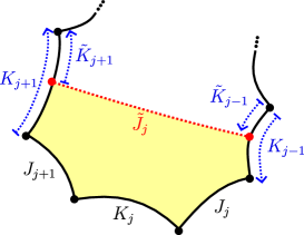
(a) One cell.

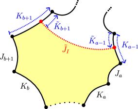
(b) Several cells.

Figure 30. Geodesic representative of a polygonal curve and of a neutralization.

Importantly, if $\Gamma^{\prime}$ is a polygonal curve derived from $\Gamma$, because $\Gamma^{\prime}$ is homotopic to $\Gamma$, we have

$$Q_{|\Gamma|}(\vec{L},\vec{\tau})=\ell_{Y}(\Gamma)=\ell_{Y}(\Gamma^{\prime})=Q_{|\Gamma^{\prime}|}(\vec{L}^{\prime},\vec{\tau}^{\prime})$$

where $\vec{L}^{\prime},\vec{\tau}^{\prime}$ are the length parameters of $\Gamma^{\prime}$. As a consequence, we obtain multiple distinct rewritings of the length of the same closed geodesic, depending on which polygonal curve we use, $\Gamma$, or any derived polygonal curve $\Gamma^{\prime}$. Our goal in the following will be to neutralize enough cells so that the expression of the length is well-behaved and can be easily understood.

We make the following observation.

Lemma 8.6.

Let $\Gamma$ be a polygonal curve of combinatorial length $m$, and $I=\{a,\ldots,b\}$ be an interval of $\mathbb{Z}_{m}$. Then,

(8.3) $$\begin{split}\tilde{L}_{I}&=\mathrm{fn}(L_{a},\ldots,L_{b+1},\tau_{a},\ldots,\tau_{b})\\ \tilde{\tau}_{a-1}&=\tau_{a-1}-\mathrm{fn}(L_{a},\ldots,L_{b+1},\tau_{a},\ldots,\tau_{b})\\ \tilde{\tau}_{b+1}&=\tau_{b+1}-\mathrm{fn}(L_{a},\ldots,L_{b+1},\tau_{a},\ldots,\tau_{b}).\end{split}$$

This is a straightforward consequence of applying the following elementary lemma to the highlighted right-angled polygon in Figure 30.

Lemma 8.7.

Let $m\geq 3$. In any right-angled convex polygon $(J_{j},K_{j})_{j\in\mathbb{Z}_{m}}$, any three consecutive lengths can be written as functions of the $2m-3$ others:

$$(\ell(K_{j}),\ell(J_{j}),\ell(K_{j+1}))=\mathrm{fn}\big{(}(\ell(J_{k}))_{k\in\mathbb{Z}_{m}\setminus\{j\}},(\ell(K_{k}))_{k\in\mathbb{Z}_{m}\setminus\{j,j+1\}}\big{)}.$$

Proof of Lemma 8.7.

When $m=3$, this is a direct consequence of the basic formulas for convex right-angled hexagons (see e.g. [5, Theorem 2.4.1 (i-ii)]). For $m>3$, we obtain the result by induction, introducing a right-angled hexagon at each step. ∎

8.4. Favorable regions for studying the length of a polygonal curve

We are now ready to study the variations of the function

(8.4) $$F_{m}(\vec{L},\vec{\tau})=\frac{1}{2}\sum_{\alpha\in\{0,1\}^{m}}(-1)^{|\alpha|}\operatorname{hyp}_{-\partial\alpha}\left(\frac{\vec{L}}{2}\right)e^{-\alpha\cdot\vec{\tau}}.$$

We observe that the first term, corresponding to $\alpha=(0,\ldots,0)$, has the coefficient

$$\operatorname{hyp}_{-1}\left(\frac{\vec{L}}{2}\right)=\prod_{j=1}^{m}\sinh\left(\frac{L_{j}}{2}\right).$$

We shall identify a “favourable” region of the Teichmüller space where this term dominates all others, so that $\cosh(\ell_{Y}(\Gamma)/2)$ is comparable to $\exp\left(\frac{1}{2}(\sum_{j=1}^{m}\tau_{j})\right)\prod_{j=1}^{m}\sinh(L_{j}/2)$.

8.4.1. Height of a cell

First, we introduce a geometric quantity associated to each cell, called its height. We will see in §8.4.2 how this is the relevant quantity one needs to introduce to describe the variations of the function $F_{m}$.

Definition 8.8.

Let $\Gamma$ be a polygonal curve of combinatorial length $m$, and $j\in\mathbb{Z}_{m}$. The height of the cell $K_{j}$ is defined as

(8.5) $$Z^{\Gamma}_{K_{j}}:=\tanh(L_{j})\tanh(L_{j+1})\,e^{\tau_{j}}.$$

We also use the short-hand notation $Z_{j}:=Z^{\Gamma}_{K_{j}}$, when convenient.

Note that, if $m=1$, the height is defined as $Z_{1}=\tanh^{2}(L_{1})e^{\tau_{1}}$. If $m=0$, the polygonal curve has no cell, so there is no notion of height.

We prove the following bounds on the height $Z_{j}$ of a cell.

Lemma 8.9.

For $m\geq 2$, $1\leq Z_{j}\leq e^{\tau_{j}}$ and upon neutralizing the cell $K_{j}$, we have

(8.6) $$\tilde{L}_{j}\leq\log Z_{j}+L_{j}+L_{j+1}.$$

Proof.

The upper bound $Z_{j}\leq e^{\tau_{j}}$ is a direct consequence of the definition. The two other bounds can be obtained from the trigonometric formula for right-angled hexagons, see e.g. [5, Theorem 2.4.1 (i)], which yield

(8.7) $$\cosh(\tilde{L}_{j})=\sinh(L_{j})\sinh(L_{j+1})\cosh(\tau_{j})-\cosh(L_{j})\cosh(L_{j+1}).$$

Indeed, $\cosh(\tilde{L}_{j})\geq 0$ together with (8.7) imply that

$$\tanh(L_{j})\tanh(L_{j+1})\cosh(\tau_{j})\geq 1$$

and hence $Z_{j}\geq 1$. Then, we rewrite (8.7) as

$$(\cosh(\tau_{j})-1)\sinh(L_{j})\sinh(L_{j+1})=\cosh(\tilde{L}_{j})+\cosh(L_{j}-L_{j+1})\geq\cosh(\tilde{L}_{j}).$$

Since $\cosh(\tau_{j})-1=2\sinh^{2}\left(\frac{\tau_{j}}{2}\right)\leq e^{\tau_{j}}/2$, this implies that

$$2\cosh(\tilde{L}_{j})\leq e^{\tau_{j}}\sinh(L_{j})\sinh(L_{j+1})=Z_{j}\cosh(L_{j})\cosh(L_{j+1})$$

which yields the result since $e^{x}/2\leq\cosh(x)\leq e^{x}$. ∎

We notice that (8.6) means that the height $Z_{j}$ of a cell $K_{j}$ can be used to bound the length $\tilde{L}_{j}$ of the roof over it, under the additional assumption that the lengths of the adjacent bridges are bounded. More generally, the height of the cell $K_{j}$ can be used to bound the length of the orthogeodesic $W_{j}$ constructed below and represented in Figure 31.

Definition 8.10.

For $j\in\mathbb{Z}_{m}$, we define the orthogeodesic $W_{j}$ by:

• $W_{j}=K_{j}$ if $L_{j}\geq 1$ and $L_{j+1}\geq 1$;

• $W_{j}$ is the orthogeodesic between $K_{j-1}$ and $J_{j+1}$ if $L_{j}<1$ and $L_{j+1}\geq 1$;

• $W_{j}$ is the orthogeodesic between $J_{j}$ and $K_{j+1}$ if $L_{j}\geq 1$ and $L_{j+1}<1$;

• $W_{j}=\tilde{J}_{j}$ otherwise, i.e. if $L_{j}<1$ and $L_{j+1}<1$.

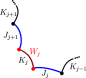
(a) $L_{j},L_{j+1}\geq 1$.

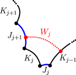
(b) $L_{j}<1$ and $L_{j+1}\geq 1$.

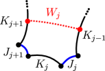
(c) $L_{j}<1$ and $L_{j+1}<1$.

Figure 31. The orthogeodesic $W_{j}$ depending on the values of $L_{j}$ and $L_{j+1}$.

We then have the following bound.

Lemma 8.11.

For any $j$, $\ell(W_{j})\leq\log(Z_{j})+2$.

Proof.

If both $L_{j}$ and $L_{j+1}$ are smaller than one, then this follows from (8.6). When both $L_{j}$ and $L_{j+1}$ are greater or equal to $1$, it is a straightforward consequence of the definition and the fact that $\log(1/\tanh(1))<1$. In the last cases, say $L_{j}<1$ and $L_{j+1}\geq 1$, we use the hyperbolic formulas for right-angles pentagons (see [5, Theorem 2.3.4 (i)]) to write $\cosh\ell(W_{j})=\sinh L_{j}\sinh\tau_{j}$, which once again yields the claim since $\log(2/\sinh(1))<1$. ∎

8.4.2. Favourable regions and estimates on $F_{m}$

We are ready to use our notion of height of a cell to identify a condition upon which the leading term of $F_{m}$ is the term $\alpha=(0,\ldots,0)$.

Lemma 8.12.

For any polygonal curve $\Gamma$ of combinatorial length $m\geq 1$, any $Y\in\mathcal{T}_{g_{\mathbf{S}},n_{\mathbf{S}}}^{*}$, any multi-index $\alpha\in\{0,1\}^{m}$ distinct from $(0,\ldots,0)$,

(8.8) $$\frac{\operatorname{hyp}_{-\partial\alpha}\left(\frac{\vec{L}}{2}\right)}{\operatorname{hyp}_{-1}\left(\frac{\vec{L}}{2}\right)}e^{-\alpha\cdot\vec{\tau}}\leq\prod_{j\in\alpha}\frac{4}{Z_{K_{j}}^{\Gamma}}.$$

In particular, if all the $Z_{j}$ go to $+\infty$, then for all $\alpha\not=(0,\ldots,0)$,

$$\frac{\operatorname{hyp}_{-\partial\alpha}\left(\frac{\vec{L}}{2}\right)}{\operatorname{hyp}_{-1}\left(\frac{\vec{L}}{2}\right)}e^{-\alpha\cdot\vec{\tau}}=o(1).$$

We can then deduce that $F_{m}(\vec{L},\vec{\tau})\sim\operatorname{hyp}_{-1}(\vec{L}/2)$ and $\cosh(\ell_{Y}(\Gamma)/2)\sim\operatorname{hyp}_{-1}\left(\frac{\vec{L}}{2}\right)\exp(\frac{1}{2}(\sum_{j=1}^{m}\tau_{j}))$, as quantified in the following statement.

Corollary 8.13.

Let $\Gamma$ be a polygonal curve of combinatorial length $m\geq 1$. For a real number $a\geq(m+3)\log 2$, if we assume

$$\forall j\in\mathbb{Z}_{m},\quad Z_{K_{j}}^{\Gamma}\geq e^{a}$$

then we have

(8.9) $$F_{m}(\vec{L},\vec{\tau})\geq\frac{1}{4}\operatorname{hyp}_{-1}\left(\frac{\vec{L}}{2}\right)\quad\text{and}\quad\cosh\left(\frac{\ell_{Y}(\Gamma)}{2}\right)\geq\frac{e^{ma/2}}{2^{m+2}}.$$

This motivates the following definitions.

Notation 8.14.

In the following, we let $a=a(r)=\max((2r+3)\log(2),2\log(8\cosh(3/2)))$, where, recall, $r$ is the number of intersections of our generalized eight. We also fix two smooth functions $\chi_{\Gamma,0},\chi_{\Gamma,\infty}$ on $\mathbb{R}$, with the property that $\chi_{\Gamma,0}$ is supported in $[-e^{a+1},e^{a+1}]$, $\chi_{\Gamma,0}\equiv 1$ on $[-e^{a},e^{a}]$, and $\chi_{\Gamma,0}+\chi_{\Gamma,\infty}\equiv 1$.

Definition 8.15.

Let $\Gamma$ be a polygonal curve of combinatorial length $m\leq 2r$. We call $\Gamma$-favourable region the region of Teichmüller space

$$\{Y\in\mathcal{T}_{g_{\mathbf{S}},n_{\mathbf{S}}}^{*}:\quad\forall j\in\mathbb{Z}_{m},Z_{K_{j}}^{\Gamma}>e^{a}\}.$$

Remark 8.16.

In particular, using Corollary 8.13 and the fact that $e^{a/2}\geq 8\cosh 3/2$, we obtain that, for any polygonal curve $\Gamma$, if $Y$ is in the $\Gamma$-favorable region, then $\ell_{Y}(\Gamma)\geq 3$.

Proof of Lemma 8.12.

Let $m\geq 2$. For $\alpha\in\{0,1\}^{m}$ such that $\alpha\neq(0,\ldots,0)$, let us write $\{j\in\mathbb{Z}_{m}:\alpha_{j}=1\}$ as a disjoint union of intervals,

$$\{j\in\mathbb{Z}_{m}:\alpha_{j}=1\}=\bigsqcup_{i=1}^{l}\{k_{i},\ldots,l_{i}\},$$

so that $\alpha_{j}=1$ for $k_{i}\leq j\leq l_{i}$ but $\alpha_{k_{i}-1}=0=\alpha_{l_{i}+1}$. Then, by definition, $(\delta\alpha)_{j}=-1$ when $j=k_{i}$ or $l_{i}+1$ and $+1$ otherwise. It follows that

$$\frac{\operatorname{hyp}_{-\partial\alpha}\left(\frac{\vec{L}}{2}\right)}{\operatorname{hyp}_{-1}\left(\frac{\vec{\vec{L}}}{2}\right)}\,e^{-\alpha\cdot\tau} =\prod_{i=1}^{l}\coth\left(\frac{L_{k_{i}}}{2}\right)\coth\left(\frac{L_{l_{i}+1}}{2}\right)\prod_{k_{i}\leq j\leq l_{i}}e^{-\tau_{j}}.$$

We note that, for all $x\geq 0$, we have $\coth(x/2)\leq 2\coth(x)$. Therefore,

$$\frac{\operatorname{hyp}_{-\partial\alpha}\left(\frac{\vec{L}}{2}\right)}{\operatorname{hyp}_{-1}\left(\frac{\vec{L}}{2}\right)}\,e^{-\alpha\cdot\tau}\leq\prod_{i=1}^{l}4\coth(L_{k_{i}})\coth(L_{l_{i}+1})\prod_{k_{i}\leq j\leq l_{i}}e^{-\tau_{j}}.$$

We then inject $1\leq\prod_{k_{i}<j\leq l_{i}}4\coth^{2}(L_{j})$ in this equation, and obtain

$$\frac{\operatorname{hyp}_{-\partial\alpha}\left(\frac{\vec{L}}{2}\right)}{\operatorname{hyp}_{-1}\left(\frac{\vec{L}}{2}\right)}\,e^{-\alpha\cdot\tau}\leq\prod_{i=1}^{l}\prod_{k_{i}\leq j\leq l_{i}}4\coth(L_{j})\coth(L_{j+1})e^{-\tau_{j}}=\prod_{j\in\alpha}\frac{4}{Z_{j}}$$

which is our claim. ∎

Proof of Corollary 8.13.

First we observe that, by hypothesis, for any $j$, $4/Z_{j}\leq 4e^{-a}\leq 2^{-m-1}$ which is smaller than $1$. As a consequence, for any $\alpha\neq(0,\ldots,0)$, we have $\prod_{j\in\alpha}4/Z_{j}\leq 2^{-m-1}$. To then deduce the bound (8.9), we write the triangle inequality:

$$F_{m}(\vec{L},\vec{\tau})\geq\frac{1}{2}\operatorname{hyp}_{-1}\left(\frac{\vec{L}}{2}\right)\Big{[}1-\sum_{\begin{subarray}{c}\alpha\in\{0,1\}^{m}\\ \alpha\not=(0,\ldots,0)\end{subarray}}\frac{\operatorname{hyp}_{-\partial\alpha}\left(\frac{\vec{L}}{2}\right)}{\operatorname{hyp}_{-1}\left(\frac{L}{2}\right)}e^{-\alpha\cdot\tau}\Big{]}\geq\frac{1}{4}\operatorname{hyp}_{-1}\left(\frac{\vec{L}}{2}\right)$$

because the sum above is bounded above by $\sum_{\begin{subarray}{c}\alpha\in\{0,1\}^{m}\end{subarray}}2^{-m-1}=1/2$. There only remains to prove the last claim, which can be obtained by writing

$$\cosh\left(\frac{\ell_{Y}(\Gamma)}{2}\right) =e^{\sum_{j=1}^{m}\tau_{j}/2}F_{m}(\vec{L},\vec{\tau})\geq\frac{1}{4}e^{\sum_{j=1}^{m}\tau_{j}/2}\prod_{j=1}^{m}\sinh\left(\frac{L_{j}}{2}\right)$$

thanks to the bound on $F_{m}$. Then, since $\sinh(x/2)\geq\tanh(x)/2$ for all $x\geq 0$,

$$\cosh\left(\frac{\ell_{Y}(\Gamma)}{2}\right)\geq\frac{1}{2^{m+2}}e^{\sum_{j=1}^{m}\tau_{j}/2}\prod_{j=1}^{m}\tanh(L_{j})=\frac{1}{2^{m+2}}\prod_{j=1}^{m}Z_{j}^{1/2}\geq\frac{e^{ma/2}}{2^{m+2}}.$$

∎

8.4.3. Derivatives of $F_{m}$

Let us now estimate the logarithmic derivatives of the function $F_{m}$ within the favorable region.

Proposition 8.17.

Let $\Gamma=(J_{j},K_{j})_{j\in\mathbb{Z}_{m}}$ be a polygonal curve of combinatorial length $m\geq 1$. If the metric $Y$ is in the $\Gamma$-favourable region, then for any subset $\pi\subseteq\mathbb{Z}_{m}$,

$$\Big{|}\prod_{j\in\pi}\frac{\partial}{\partial\tau_{j}}\big{(}\log F_{m}\big{)}(\vec{L},\vec{\tau})\Big{|}\leq\mathrm{fn}(m)\,\prod_{j\in\pi}\frac{1}{Z_{j}}.$$

Proof.

Let $k=\#\pi$. The partial derivative $\partial^{\pi}\log F_{m}$ is a linear combination (with universal coefficients depending only on $k$) of fractions of the form $\prod_{j=1}^{k}(\partial^{\pi_{j}}F_{m}/F_{m})$ where the non-empty subsets $\pi_{1},\ldots,\pi_{k}$ of $\mathbb{Z}_{m}$ form a partition of $\pi$. We then write for each $j\in\{1,\ldots,k\}$

$$\frac{\partial^{\pi_{j}}F_{m}}{F_{m}}=\sum_{\alpha\in\{0,1\}^{m}}(-1)^{|\alpha|}\frac{\operatorname{hyp}_{-\partial\alpha}\left(\frac{\vec{L}}{2}\right)\partial^{\pi_{j}}(e^{-\alpha\cdot\vec{\tau}})}{F_{m}}.$$

To bound the denominator, we use (8.9), which states that $F_{m}(\vec{L},\vec{\tau})\geq\frac{1}{4}\operatorname{hyp}_{-1}(\vec{L}/2)$. For the numerator, we note that $\partial^{\pi_{j}}(e^{-\alpha\cdot\vec{\tau}})=0$ unless $\alpha_{i}=1$ for all $i\in\pi_{j}$, and in the latter case we have $\partial^{\pi_{j}}(e^{-\alpha\cdot\vec{\tau}})=(-1)^{\#\pi_{j}}e^{-\alpha\cdot\vec{\tau}}$. In particular, the term $\alpha=(0,\ldots,0)$ does not contribute to the sum. Then,

$$\left|\frac{\partial^{\pi_{j}}F_{m}}{F_{m}}\right|\leq 4\sum_{\begin{subarray}{c}\alpha\in\{0,1\}^{m}\\ \alpha\neq(0,\ldots,0)\end{subarray}}\frac{\operatorname{hyp}_{-\partial\alpha}\left(\frac{\vec{L}}{2}\right)e^{-\alpha\cdot\vec{\tau}}}{\operatorname{hyp}_{-1}\left(\frac{\vec{L}}{2}\right)}\leq 2^{3m+2}\prod_{i\in\pi_{j}}\frac{1}{Z_{i}}$$

by Lemma 8.12, using the fact that there are at most $2^{m}$ terms in the sum. Taking the product over $j=1,\ldots,k$ yields

$$\prod_{j=1}^{k}\left|\frac{\partial^{\pi_{j}}F_{m}}{F_{m}}\right|\leq 2^{(3m+2)k}\prod_{i\in\pi}\frac{1}{Z_{i}}.$$

Summing over all partitions $\pi_{1},\ldots,\pi_{k}$ of $\pi$, and noticing that $k\leq m$, yields the announced bound. ∎

8.4.4. Decoration for one polygonal curve

We recall that our aim in this section is to provide a well-described formula for the length of a polygonal curve $\Gamma$. Proposition 8.17 tells us that this is achieved as soon as our metric $Y$ lies in the $\Gamma$-favorable region. If this is not the case, then we shall replace $\Gamma$ by a derived polygonal curve $\Gamma^{\prime}$ obtained by neutralizing a cell $K$ such that $Z_{K}^{\Gamma}\leq e^{a}$, and hope that $Y$ now falls in the $\Gamma^{\prime}$-favourable region. Since the combinatorial length strictly decreases under derivation, we can iterate this process finitely many times until we reach a favourable region for a polygonal curve $\Gamma^{\prime\prime}$ derived from $\Gamma$. Since $\Gamma^{\prime\prime}$ is homotopic to $\Gamma$, this yields a well-behaved formula for the length $\ell_{Y}(\Gamma)$ in terms of the lengths of the cells and bridges of $\Gamma^{\prime\prime}$.

The decorations, defined below, will serve to enumerate all possible cases in this recursive process. Later on (§8.6), decorations will be used to construct a partition of unity on the Teichmüller space: a decoration $\infty$ on a cell $K$ will mean that we consider the region of Teichmüller space where the height $Z^{\Gamma}_{K}$ is high, and on the opposite the decoration $0$ will mean that we consider the region where the height $Z^{\Gamma}_{K}$ is low.

Let us provide the general definition of a decoration for a polygonal curve $\Gamma$.

Definition 8.18.

A decorated polygonal curve $(\Gamma,d)$ is a polygonal curve $\Gamma$ of combinatorial length $|\Gamma|\geq 1$, together with a map $d:\operatorname{Cell}(\Gamma)\longrightarrow\{0,\infty\}$. A cell $K\in\operatorname{Cell}(\Gamma)$ is called favourable if $d(K)=\infty$ and unfavourable if $d(K)=0$. A decorated polygonal curve $(\Gamma,d)$ is called favourable if all cells are favourable.

A decorated polygonal curve $(\Gamma^{\prime},d^{\prime})$ is said to be derived from $(\Gamma,d)$ if $\Gamma^{\prime}$ is derived from $\Gamma$ by neutralizing a cell $K\in\operatorname{Cell}(\Gamma)$ such that $d(K)=0$. In addition, we ask that the map $d^{\prime}$ coincides with $d$ on $\operatorname{Cell}(\Gamma^{\prime})\cap\operatorname{Cell}(\Gamma)$.

The following definition allows us to consider the iterative derivation process described above.

Definition 8.19.

Let $\Gamma$ be a polygonal curve. An exhaustion for $\Gamma$ is a sequence of decorated polygonal curves $(\mathbf{\Gamma},\mathbf{d})=(\Gamma^{k},d^{k})_{1\leq k\leq t}$, such that

• $\Gamma^{1}=\Gamma$;

• for every $k<t$, $(\Gamma^{k},d^{k})$ is not favourable, and $(\Gamma^{k+1},d^{k+1})$ is derived from $(\Gamma^{k},d^{k})$;

• for $k=t$, $(\Gamma^{t},d^{t})$ is either favourable or of combinatorial length $=0$.

Remark 8.20.

In particular, any polygonal curve of combinatorial length $0$ is left untouched by the exhaustion process. It follows that, if we apply this process to a polygonal curve $\beta_{\lambda}$ with $\lambda\in\Lambda^{\beta}$ (i.e. a component of $\beta$), then nothing happens.

Notation 8.21.

For an exhaustion $(\mathbf{\Gamma},\mathbf{d})=(\Gamma^{k},d^{k})_{1\leq k\leq t}$ of a polygonal curve $\Gamma$, we denote as $(\Gamma^{\infty},d^{\infty})=(\Gamma^{t},d^{t})$ the decorated polygonal curve at the terminal step of the exhaustion.

8.5. Families of polygonal curves and simultanous decorations

The integral (5.13), our main focus, simultanously involves all the lengths $(\ell_{Y}(\Gamma_{\lambda}))_{\lambda\in\Lambda}$ through the function ${\mathchoice{1\mskip-4.0mu{\rm{l}}}{1\mskip-4.0mu{\rm{l}}}{1\mskip-4.5mu{\rm{l}}}{1\mskip-5.0mu{\rm{l}}}}_{\mathfrak{D}}$. We will therefore need to consider simultaneously all the polygonal curves $(\Gamma_{\lambda})_{\lambda\in\Lambda}$. This motivates the need to study families of polygonal curves, which we do in this section.

In the following, our families are indexed by our set $\Lambda$ introduced in §3.3 to index our pair of pants decomposition, but the precise structure of $\Lambda$ does not matter. The one thing that is important is that we have ordered the set $\Lambda$ with the order relation $\lambda_{1}<\lambda_{2}$ if $\operatorname{step}(\lambda_{1})<\operatorname{step}(\lambda_{2})$, where $\operatorname{step}(\lambda)$ is the step of the construction of the pair of pants decomposition at which $\Gamma_{\lambda}$ appears. The considerations below can be applied to any partially ordered set $\Lambda$.

8.5.1. Compatibility of polygonal curves

When considering families of polygonal curves, we will need to understand how the different polygonal curves in our family intersect one another. Without any hypothesis, two polygonal curves can have quite wild intersections and combinatorics. The following notion of compatibility will be key to restrict the possible behaviours and describe our families of polygonal curves.

Definition 8.22 (Compatibility of two polygonal curves).

Let $\Gamma_{1}$, $\Gamma_{2}$ be two polygonal curves based on $\beta$. We say that $\Gamma_{1}$ and $\Gamma_{2}$ are compatible if:

• if two cells $K^{1}\in\operatorname{Cell}(\Gamma_{1})$, $K^{2}\in\operatorname{Cell}(\Gamma_{2})$ lie in the same component of $\beta$ and have the same orientation, then they are either disjoint or one is included in the other;

• two bridges $J^{1}\in\operatorname{Br}(\Gamma_{1})$, $J^{2}\in\operatorname{Br}(\Gamma_{2})$ are either equal or disjoint (in particular, they cannot have an endpoint in common unless they are equal).

As a consequence of our definition of polygonal curves, for any cells $K^{1},K^{2}$ within one component $\beta$ and oriented the same way, the bridges adjacent to $K^{1}$ and $K^{2}$ all lie on the same side of that component of $\beta$. The compatibility condition then implies that any two compatible polygonal curves $\Gamma_{1}$ and $\Gamma_{2}$ are homotopic to simple curves not intersecting one another.

Definition 8.23 (Inclusion of cells).

Let $\Gamma_{1}$, $\Gamma_{2}$ be two compatible polygonal curves. Let $K^{1}\in\operatorname{Cell}(\Gamma_{1})$ and $K^{2}\in\operatorname{Cell}(\Gamma_{2})$ be two cells of $\Gamma_{1}$, $\Gamma_{2}$ respectively. We say that the cell $K^{1}$ is included in the cell $K^{2}$, and write $K^{1}\subseteq K^{2}$, if $K^{1}$ is a subset of $K^{2}$ and their orientations are the same. We will say that the two cells coincide, and write $K^{1}=K^{2}$, if $K^{1}\subseteq K^{2}$ and $K^{2}\subseteq K^{1}$. In this case, we say that $\Gamma_{1}$ and $\Gamma_{2}$ have a cell in common. We say that $K^{1}$ is strictly included in $K^{2}$, and write $K^{1}\subsetneq K^{2}$, if $K^{1}\subseteq K^{2}$ and $K_{1}\neq K_{2}$.

Because of the second item in Definition 8.22, if $K^{1}=K^{2}$, then the bridges adjacent to this common cell are equal.

Remark 8.24.

The reason we insist on only comparing cells with the same orientation is that we want the notion of inclusion to be purely topological, that is, independent on the choice of a hyperbolic metric. If $K^{1}\subseteq K^{2}$ for topological polygonal curves $\Gamma_{1},\Gamma_{2}$, then, by the Useful Remark 2.11, we have that the geodesic representatives $\bar{K}^{1}$ and $\bar{K}^{2}$ satisfy $\bar{K}^{1}\subseteq\bar{K}^{2}$ in the sense of the inclusion of sets.

Definition 8.25.

We say a family of polygonal curves $(\Gamma_{\lambda})_{\lambda\in\Lambda}$ form a compatible family if

• these polygonal curves are pairwise compatible;

• for $K^{1}\in\operatorname{Cell}(\Gamma_{\lambda_{1}})$ and $K^{2}\in\operatorname{Cell}(\Gamma_{\lambda_{2}})$, if $K^{1}\subsetneq K^{2}$, then $\lambda_{2}<\lambda_{1}$.

Example 8.26.

By construction, the family $(\Gamma_{\lambda})_{\lambda\in\Lambda}$ of boundary components of our pair of pants decomposition is a compatible family of polygonal curves.

Notation 8.27.

For $\Gamma=(\Gamma_{\lambda})_{\lambda\in\Lambda}$ a compatible family of polygonal curves, we let

$$\operatorname{Cell}(\Gamma)=\bigcup_{\lambda\in\Lambda}\operatorname{Cell}(\Gamma_{\lambda}),$$

where the union runs over the $\lambda\in\Lambda$ such that $|\Gamma_{\lambda}|\geq 1$. For $K\in\operatorname{Cell}(\Gamma)$, if $\lambda\in\Lambda$ is such that $K\in\operatorname{Cell}(\Gamma_{\lambda})$, then we denote by $\tilde{J}(K)$ the roof over $K$ in $\Gamma_{\lambda}$ and $Z_{K}^{\Gamma}:=Z_{K}^{\Gamma_{\lambda}}$ the height of $K$. We call complexity of $\Gamma$, and denote $|\Gamma|$, its number of cells.

Thanks to the compatibility condition, $\tilde{J}(K)$ and $Z_{K}^{\Gamma}$ do not depend on the choice of a $\lambda\in\Lambda$ for which $K\in\operatorname{Cell}(\Gamma_{\lambda})$. The following property will allow us to compare heights within a compatible family. It says that the height is (almost) increasing for the inclusion relation.

Proposition 8.28.

Consider a compatible family $\Gamma=(\Gamma_{\lambda})_{\lambda\in\Lambda}$. Let $K,K^{\prime}\in\operatorname{Cell}(\Gamma)$, such that $K^{\prime}\subseteq K$. Then

(8.10) $$Z_{K}^{\Gamma}\geq e^{-2}Z_{K^{\prime}}^{\Gamma}.$$

Proof.

Let us lift the polygonal curve to the hyperbolic plane. Let $K$ and $K^{\prime}$ denote two lifts of our cells, such that $K^{\prime}\subseteq K$. Let $J_{-}$, $J_{+}$ denote lifts of the bridges arriving on $K$ and coming out of $K$, and similarly $J_{-}^{\prime}$, $J_{+}^{\prime}$ for $K^{\prime}$. By definition of the inclusion of cells, all of those bridges lie on the same side of $K$. We denote as $L_{\pm}$ and $L_{\pm}^{\prime}$ the lengths of these bridges, and $\tau$, $\tau^{\prime}$ the lengths of the cells $K$, $K^{\prime}$.

Let $t_{\pm}$ denote the distance between the origins of $J_{\pm}$ and $J_{\pm}^{\prime}$ along $K$. We shall only prove the property when $t_{+},t_{-}>0$, i.e. the bridges $J_{\pm}$ and $J_{\pm}^{\prime}$ are disjoint – the proof is simpler when one or both of these lengths is equal to $0$.

Let $\tilde{\beta}_{+}$, $\tilde{\beta}_{+}^{\prime}$ denote the lifts of the multicurve $\beta$ on which the bridges $J_{+}$, $J_{+}^{\prime}$ terminate. Since there is no right-angled quadrilateral in $\mathbb{H}$, these two lifts must differ. Then, completing the picture with the orthogeodesic between $\beta_{+}$ and $\beta_{+}^{\prime}$, we obtain a convex right-angled hexagon, see Figure 32.

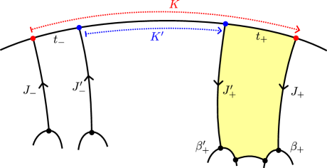
Figure 32. Illustration of the proof of Proposition 8.28.

In a convex right-angled hexagon, the lengths $\ell_{1},\ell_{2}$ of any two consecutive edges must satisfy $\sinh(\ell_{1})\sinh(\ell_{2})\geq 1$. Indeed, one can cut the hexagon along one of its orthogeodesics to obtain a right-angled pentagon with two consecutive edges of lengths $\ell_{1},\ell_{2}$, which then must satisfy the aforementioned inequality by [5, Therorem 2.3.4(i)].

It then follows that $\sinh(t_{+})\sinh(L_{+})\geq 1$. If $L_{+}\leq 1$, then $\sinh(L_{+})\geq\tanh(L_{+})/e$ and we hence obtain

(8.11) $$e^{t_{+}}\tanh(L_{+})\geq 1/e.$$

Otherwise, $e^{t_{+}}\geq 1$ and $\tanh(L_{+})\geq\tanh(1)\geq 1/e$, so the inequality (8.11) also holds. By symmetry, (8.11) remains true replacing all $+$ by $-$.

Then, we write $\tau=\tau^{\prime}+t_{+}+t_{-}$, and hence

$$Z_{K}^{\Gamma}=\tanh(L_{+})\tanh(L_{-})\,e^{\tau^{\prime}+t_{+}+t_{-}}\geq\frac{e^{\tau^{\prime}}}{e^{2}}\geq e^{-2}\tanh(L_{+}^{\prime})\tanh(L_{-}^{\prime})e^{\tau^{\prime}}=e^{-2}Z_{K^{\prime}}^{\Gamma}$$

which was our claim. ∎

8.5.2. Neutralization in a compatible family

In §8.2.2, we defined a notion of neutralization of a cell $K$ for a single polygonal curve. Now, we define and discuss the notion of neutralization of a cell $K$ in a compatible family of polygonal curves $\Gamma=(\Gamma_{\lambda})_{\lambda\in\Lambda}$.

Definition 8.29.

Let $\Gamma=(\Gamma_{\lambda})_{\lambda\in\Lambda}$ be a family of polygonal curves. Let $K\in\operatorname{Cell}(\Gamma)$.

For every $\lambda\in\Lambda$, we let $\Gamma^{\prime}_{\lambda}$ be the polygonal curve derived from $\Gamma_{\lambda}$ by simultaneously neutralizing all cells $K^{\prime}\in\operatorname{Cell}(\Gamma_{\lambda})$ such that $K^{\prime}\subseteq K$. We say that the family $\Gamma^{\prime}=(\Gamma^{\prime}_{\lambda})_{\lambda\in\Lambda}$ is derived from $\Gamma$ by neutralizing $K$.

We show, using the Useful Remark, that the notion of compatibility is stable by derivation.

Proposition 8.30.

If $\Gamma$ is a compatible family and $\Gamma^{\prime}$ is derived from $\Gamma$ by neutralizing a cell, then $\Gamma^{\prime}$ is a compatible family.

Proof.

Let $\tilde{K}^{1},\tilde{K}^{2}\in\operatorname{Cell}(\Gamma^{\prime})$ be two cells with non-empty intersection and oriented the same way. We wish to prove that either $\tilde{K}^{1}\subseteq\tilde{K}^{2}$ or $\tilde{K}^{2}\subseteq\tilde{K}^{1}$, and that the bridges adjacent to these cells are equal or disjoint.

For $i=1,2$, let $\lambda_{i}\in\Lambda$ denote an index for which $\tilde{K}^{i}\in\Gamma^{\prime}_{\lambda_{i}}$. By definition, $\Gamma^{\prime}_{\lambda_{i}}$ is derived from $\Gamma_{\lambda_{i}}$ by neutralizing some cells, and therefore the cell $\tilde{K}^{i}$ is contained in a cell $K^{i}$ of $\Gamma_{\lambda_{i}}$.

By the compatibility condition, two lifts of $\Gamma_{\lambda_{1}}$ and $\Gamma_{\lambda_{2}}$ to $\mathbb{H}^{2}$ cannot intersect transversally. Consider two such lifts, say $(J_{j}^{1},K_{j}^{1})_{j\in\mathbb{Z}}$ and $(J^{2}_{j},K^{2}_{j})_{j\in\mathbb{Z}}$, chosen so that $K_{0}^{1}$ and $K_{0}^{2}$ are respective lifts of $K^{1}$ and $K^{2}$ and $K_{0}^{1}\cap K_{0}^{2}\neq\emptyset$.

Let us consider the index

$$m=\inf\{j\geq 0:t(K^{1}_{j})\not=t(K^{2}_{j})\},$$

i.e. the first place where the two polygonal curves $\Gamma_{\lambda_{1}}$ and $\Gamma_{\lambda_{2}}$ start disagreeing after meeting along $K_{0}^{1}$ and $K_{0}^{2}$ (see Figure 33). First, we observe that if $m=+\infty$, then $\Gamma_{\lambda_{1}}=\Gamma_{\lambda_{2}}$ and thus $\Gamma^{\prime}_{\lambda_{1}}=\Gamma^{\prime}_{\lambda_{2}}$, which is enough to conclude.

If now $m<\infty$, then $J^{1}_{j}=J^{2}_{j}$ for all $j\in\{1,\ldots,m\}$. Thus, if $m>0$, then $K^{1}_{m}$ and $K^{2}_{m}$ have the same origin and, in particular, $K^{1}_{m}$ and $K_{m}^{2}$ are two distinct cells, with an intersection and oriented the same way. This is obvisouly also true by hypothesis if $m=0$. Now, because $\Gamma_{\lambda_{1}}$ and $\Gamma_{\lambda_{2}}$ are compatible, we either have $K_{m}^{2}\subsetneq K_{m}^{1}$ and $\lambda_{1}<\lambda_{2}$, or $K_{m}^{1}\subsetneq K_{m}^{2}$ and $\lambda_{2}<\lambda_{1}$ – let us assume w.l.o.g. that we are in the first situation.

If we now consider the index

$$n=\sup\{j\leq 0,o(K^{1}_{j})\not=o(K_{j}^{2})\},$$

since we assumed that $m<+\infty$, $\Gamma_{\lambda_{1}}\neq\Gamma_{\lambda_{2}}$, and hence $n>-\infty$. By the same reasoning as above, the cells $K_{n}^{1}$ and $K_{n}^{2}$ are distinct, with an intersection, and oriented the same way. Since we have now specified that $\lambda_{1}<\lambda_{2}$, we must have $K_{n}^{2}\subsetneq K_{n}^{1}$.

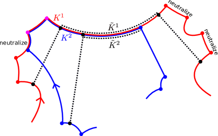
Figure 33. Example of two compatible polygonal curves under a neutralization procedure. The full lines are the initial polygonal curves. The dotted lines are the new cells $\tilde{K}^{1}$ and $\tilde{K}^{2}$ that we need to compare, and the dashed lines the new bridges. On this example, we have $m=0$ and $n=-1$.

Because two lifts of $\Gamma_{\lambda_{1}}$ and $\Gamma_{\lambda_{2}}$ cannot cross transversally, our lift of $\Gamma_{\lambda_{2}}$ then lies entirely on the right of our lift of $\Gamma_{\lambda_{1}}$, as represented in Figure 33.

Now, for $i=1,2$, let $\tilde{J}^{i}$ denote the bridge coming out of $\tilde{K}^{i}$ in $\Gamma_{\lambda_{i}}^{\prime}$. By definition of the neutralization procedure, the bridge $\tilde{J}^{i}$ is the orthogeodesic between the cell $K^{i}_{0}$ and a cell $K_{j_{i}}^{i}$ for an index $j_{i}\geq 0$, and the cells $K_{j}^{i}$ for $0<j<j_{i}$ are neutralized. There are now two cases to consider.

• If $j_{2}\geq m$, we can use the Useful Remark 2.11 to deduce that the origin of $\tilde{J}^{2}$ lies on the right of the origin of $\tilde{J}^{1}$ on $K_{0}^{1}$, and the bridges $\tilde{J}^{1}$ and $\tilde{J}^{2}$ are equal or do not cross, which is exactly our claim.

• Otherwise, $j_{2}<m$, or, in other words, the two polygonal curves $\Gamma_{\lambda_{1}}$ and $\Gamma_{\lambda_{2}}$ coincide up until the index $j_{2}$. By definition of the neutralization for a family of curve, if a cell $K^{2}_{j}$ of $\Gamma_{\lambda_{2}}$ is contained in a cell $K_{j}^{1}$ of $\Gamma_{\lambda_{1}}$ and if $K_{j}^{1}$ is neutralized, then $K^{2}_{j}$ must also be neutralized. Therefore, $j_{1}\leq j_{2}$, and we can once again use the Useful Remark to conclude.

The same reasoning also allows to prove that the origin $o(\tilde{K}^{2})$ lies on the left of $o(\tilde{K}^{1})$, and the bridges arriving on $\tilde{K}^{1}$ and $\tilde{K}^{2}$ are equal or disjoint. ∎

8.5.3. Simultaneous decoration

We are now ready to extend the notion of decoration introduced in §8.4.4 to families of polygonal curves.

Definition 8.31.

Let $\Gamma=(\Gamma_{\lambda})_{\lambda\in\Lambda}$ be a compatible family of polygonal curves. A (simultaneous) decoration of $\Gamma$ is a map $d:\operatorname{Cell}(\Gamma)\longrightarrow\{0,\infty\}$ such that any cell common to several $\Gamma_{\lambda}$ bears only one decoration.

Definition 8.32.

Let $(\Gamma,d)$ be a decorated family. A cell $K\in\operatorname{Cell}(\Gamma)$ is called unfavourable (for the decoration $d$) if $d(K)=0$ or if $K\subseteq K^{\prime}$ with $d(K^{\prime})=0$. It is called favourable otherwise. A maximal unfavourable cell is a cell which is unfavourable and maximal for inclusion.

A simultaneous decoration $d$ of the family $\Gamma$ is called favourable if all its cells are favourable.

By convention, recall that polygonal curves of combinatorial length $0$ have no cells. As a consequence, if $\Gamma=(\Gamma_{\lambda})_{\lambda\in\Lambda}$ contains only polygonal curves such that $|\Gamma_{\lambda}|=0$, then $\operatorname{Cell}(\Gamma)=\emptyset$ and in particular $\Gamma$ is favorable.

Definition 8.33.

A decorated family $(\Gamma^{\prime},d^{\prime})$ is said to be derived from $(\Gamma,d)$ if $\Gamma^{\prime}$ is derived from $\Gamma$ by neutralizing a maximal unfavourable cell and the map $d^{\prime}$ coincides with $d$ on all cells in common between $\Gamma$ and $\Gamma^{\prime}$.

Definition 8.34.

Let $\Gamma=(\Gamma_{\lambda})_{\lambda\in\Lambda}$ be a compatible family of polygonal curves. An exhaustion of $\Gamma$ is a sequence of decorated families $(\mathbf{\Gamma},\mathbf{d})=(\Gamma^{k},d^{k})_{1\leq k\leq t}$, where:

• $\Gamma^{1}=\Gamma$;

• for every $1\leq k\leq t$, $\Gamma^{k}=(\Gamma^{k}_{\lambda})_{\lambda\in\Lambda}$ is a compatible family of polygonal curves;

• for every $1\leq k<t$, $(\Gamma^{k},d^{k})$ is not favourable, and $(\Gamma^{k+1},d^{k+1})$ is derived from $(\Gamma^{k},d^{k})$;

• for $k=t$, $(\Gamma^{t},d^{t})$ is favourable.

We let $\operatorname{Cell}(\mathbf{\Gamma})=\bigcup_{k=1}^{t}\operatorname{Cell}(\Gamma^{k})$. We denote as $|\mathbf{\Gamma}|=\#\operatorname{Cell}(\mathbf{\Gamma})$ the complexity of the exhaustion $\mathbf{\Gamma}$. If $K\in\operatorname{Cell}(\mathbf{\Gamma})$, we denote $\mathbf{d}(K)=d^{k}(K)$ for any $k$ such that $K\in\operatorname{Cell}(\Gamma^{k})$.

Note that, by construction, the value of the decoration $\mathbf{d}(K)=d^{k}(K)$ is independent from the choice of an index $k$ such that $K\in\operatorname{Cell}(\Gamma^{k})$. This is also true of the roof over a cell $\tilde{J}(K)$ and height of a cell $Z_{K}^{\mathbf{\Gamma}}$ introduced in Notation 8.27.

Notation 8.35 (Terminal cells).

Let $(\mathbf{\Gamma},\mathbf{d})=(\Gamma^{k},d^{k})_{1\leq k\leq t}$ be a sequence of decorated families of polygonal curves. We denote as $(\Gamma^{\infty},d^{\infty})$ the decorated polygonal curve $(\Gamma^{t},d^{t})$. The cells of the last family $\Gamma^{\infty}$ are called the terminal cells of $(\mathbf{\Gamma},\mathbf{d})$. The set of terminal cells associated with $(\mathbf{\Gamma},\mathbf{d})$ is denoted $\mathrm{Term}({\mathbf{\Gamma}},{\mathbf{d}})$, in other words

$$\mathrm{Term}({\mathbf{\Gamma}},{\mathbf{d}}):=\operatorname{Cell}(\Gamma^{\infty}).$$

8.6. Another partition of unity on Teichmüller space

Let us now focus on our compatible family of polygonal curves $\Gamma=(\Gamma_{\lambda})_{\lambda\in\Lambda}$ defined as the boundary components of the pair of pants decomposition introduced in §3.2.

We recall that we have fixed a cutoff value $a=a(r)$ and associated cutoff functions $\chi_{\Gamma,0},\chi_{\Gamma,\infty}$ such that $\chi_{\Gamma,0}+\chi_{\Gamma,\infty}=1$ in Notation 8.14.

Notation 8.36.

Let $({\mathbf{\Gamma}},{\mathbf{d}})=(\Gamma^{k},d^{k})_{1\leq k\leq t}$ be an exhaustion of the family $(\Gamma_{\lambda})_{\lambda\in\Lambda}$. For a hyperbolic metric $Y\in\mathcal{T}_{g_{\mathbf{S}},n_{\mathbf{S}}}^{*}$, we let

(8.12) $$\Psi_{{\mathbf{\Gamma}},{\mathbf{d}}}(Y):=\prod_{K\in\operatorname{Cell}(\mathbf{\Gamma})}\chi_{\Gamma,\mathbf{d}(K)}({Z^{\mathbf{\Gamma}}_{K}}).$$

The function $\Psi_{{\mathbf{\Gamma}},{\mathbf{d}}}$ is a cut-off function on the Teichmüller space $\mathcal{T}^{*}_{g_{\mathbf{S}},n_{\mathbf{S}}}$. It achieves our purpose described throught this section. Indeed, if $Y\in\mathcal{T}_{g_{\mathbf{S}},n_{\mathbf{S}}}^{*}$ lies in the support of $\Psi_{\mathbf{\Gamma},\mathbf{d}}$, then for any cell $K\in\operatorname{Cell}(\mathbf{\Gamma})$,

• if $\mathbf{d}(K)=0$, then $Z_{K}^{\mathbf{\Gamma}}\leq e^{a+1}$;

• if $\mathbf{d}(K)=\infty$, then $Z_{K}^{\mathbf{\Gamma}}\geq e^{a}$.

We can extract from the family of functions $\Psi_{{\mathbf{\Gamma}},{\mathbf{d}}}$ with $(\mathbf{\Gamma},\mathbf{d})$ an exhaustion a partition of unity on Teichmüller space :

Proposition 8.37.

There exists a family of exhaustions $\mathfrak{E}$ of the family $(\Gamma_{\lambda})_{\lambda\in\Lambda}$ such that

(8.13) $$\forall Y\in\mathcal{T}_{g_{\mathbf{S}},n_{\mathbf{S}}}^{*},\quad\sum_{({\mathbf{\Gamma}},{\mathbf{d}})\in\mathfrak{E}}\Psi_{{\mathbf{\Gamma}},{\mathbf{d}}}(Y)=1.$$

We omit the proof, a tedious but surpriseless recursive procedure on the number of cells of the family of polygonal curves $(\Gamma_{\lambda})_{\lambda\in\Lambda}$.

8.7. Neutral variables associated with $({\mathbf{\Gamma}},{\mathbf{d}})$.

Fix an exhaustion $({\mathbf{\Gamma}},{\mathbf{d}})=(\Gamma^{k},d^{k})_{1\leq k\leq t}$ of the family $(\Gamma_{\lambda})_{\lambda\in\Lambda}$ of boundary components of our pair of pants decomposition of $\mathbf{S}$. On the support of $\Psi_{{\mathbf{\Gamma}},{\mathbf{d}}}$, we shall enlarge the set of neutral variables originally defined in §5.3, and hence diminish the number of variables with respect to which we need to apply the operator $\mathcal{L}$ under the integral (5.13).

Amongst the terminal cells of $(\mathbf{\Gamma},\mathbf{d})$, some are particularly important.

Notation 8.38.

We denote as $\mathrm{Term}_{\mathrm{BC}}(\mathbf{\Gamma},\mathbf{d})\subseteq\mathrm{Term}(\mathbf{\Gamma},\mathbf{d})$ the set of cells of $(\Gamma_{\lambda}^{\infty})_{\lambda\in\Lambda_{\mathrm{BC}}^{\Gamma}}$. We call these cells boundary terminal cells.

We observe that, by definition of the neutralization procedure, any $K\in\mathrm{Term}_{\mathrm{BC}}(\mathbf{\Gamma},\mathbf{d})$ is included in a cell of the initial polygonal curve $(\Gamma_{\lambda}^{1})_{\lambda\in\Lambda_{\mathrm{BC}}^{\Gamma}}$. The cells of this family are amongst the segments $(\mathcal{K}_{q})_{q\in\Theta}$ defined in §4.3. We also note that each segment $(\mathcal{K}_{q})_{q\in\Theta}$ can contain at most one boundary terminal cell.

We now recall that, in §4.3, we have defined for each $q\in\Theta$ a set $\Theta_{\tau}(q)\subseteq\Theta$ such that we can write the length $\tau_{q}$ of $\mathcal{K}_{q}$ as $\tau_{q}=\sum_{q^{\prime}\in\Theta_{\tau}(q)}\theta_{q^{\prime}}$.

Definition 8.39.

Let $q\in\Theta$. We call $\mathcal{K}_{q}$ a surviving boundary segment if $\mathcal{K}_{q}$ contains a boundary terminal cell. In that case, we let

(8.14) $$Z_{{\mathbf{\Gamma}},{\mathbf{d}}}(\mathcal{K}_{q}):=Z_{K}^{{\mathbf{\Gamma}}}$$

where $K$ is the unique boundary terminal cell contained in $\mathcal{K}_{q}$. We denote as $\Theta_{\mathrm{surv}}$ the set of indices $q\in\Theta$ such that $\mathcal{K}_{q}$ is a surviving boundary segment and $\vec{\tau}_{\mathrm{surv}}=(\tau_{q})_{q\in\Theta_{\mathrm{surv}}}$.

Notation 8.40.

We define additional neutral variables associated to the exhaustion $(\mathbf{\Gamma},\mathbf{d})$,

(8.15) $$\Theta_{\mathrm{nt}}({\mathbf{\Gamma}},{\mathbf{d}}):=\bigcup_{q\in\Theta\setminus\Theta_{\mathrm{surv}}}\Theta_{\tau}(q).$$

For a vector $\vec{\theta}\in\mathbb{R}^{\Theta}$, we denote as $\vec{\theta}_{\mathrm{nt}}({\mathbf{\Gamma}},{\mathbf{d}})=(\theta_{q})_{q\in\Theta_{\mathrm{nt}}({\mathbf{\Gamma}},{\mathbf{d}})}\in\mathbb{R}^{\Theta_{\mathrm{nt}}(\mathbf{\Gamma},\mathbf{d})}$ the restriction of the vector $\vec{\theta}$ to the indices in $\Theta_{\mathrm{nt}}({\mathbf{\Gamma}},{\mathbf{d}})$.

Remark 8.41.

If a boundary component $\lambda\in\Lambda_{\mathrm{BC}}$ is reduced in the exhaustion procedure to a component of combinatorial length $0$, i.e. if $|\Gamma^{\infty}_{\lambda}|=0$, then all variables $\theta_{q}$ with $\lambda(q)=\lambda$ are neutral variables.

Lemma 8.6 allows us to draw the following observations as to the variables appearing in a terminal polygonal curve.

Lemma 8.42.

Let $(\mathbf{\Gamma},\mathbf{d})$ be an exhaustion of $(\Gamma_{\lambda})_{\lambda\in\Lambda}$. Then,

• for any $q\in\Theta_{\mathrm{surv}}$, if $K$ is the unique boundary terminal cell contained in $\mathcal{K}_{q}$,

  (8.16) $$\tau_{q}=\ell(K)+\mathrm{fn}(\vec{L},\vec{\theta}_{\mathrm{nt}}({\mathbf{\Gamma}},{\mathbf{d}}));$$

• any bridge $J\in\operatorname{Br}(\Gamma^{\infty})$ of the terminal family of polygonal curves $\Gamma^{\infty}$ satisfies

  (8.17) $$\ell(J)=\mathrm{fn}(\vec{L},\vec{\theta}_{\mathrm{nt}}({\mathbf{\Gamma}},{\mathbf{d}})).$$

8.8. Structure and derivatives of the function $\Psi_{{\mathbf{\Gamma}},{\mathbf{d}}}(Y)$

Later on, we will need to be able to estimate the derivatives of the function $\Psi_{{\mathbf{\Gamma}},{\mathbf{d}}}(Y)$ with respect to certain variables. We prove the following.

Proposition 8.43.

We can rewrite $\Psi_{\mathbf{\Gamma},\mathbf{d}}(Y)$ under the form

$$\Psi_{\mathbf{\Gamma},\mathbf{d}}(Y)=\tilde{\Psi}_{\mathbf{\Gamma},\mathbf{d}}(\vec{\tau},\vec{L},\vec{\theta}_{\mathrm{nt}}(\mathbf{\Gamma},\mathbf{d}))$$

for a smooth function $\tilde{\Psi}_{\mathbf{\Gamma},\mathbf{d}}:\mathbb{R}_{>0}^{\Theta}\times\mathbb{R}_{>0}^{r}\times\mathbb{R}^{\Theta_{\mathrm{nt}}(\mathbf{\Gamma},\mathbf{d})}\rightarrow\mathbb{R}$ satisfying, for any set $\tilde{\pi}\subseteq\Theta$,

$$\Big{|}\frac{\partial^{|\tilde{\pi}|}\tilde{\Psi}_{\mathbf{\Gamma},\mathbf{d}}}{\prod_{q\in\tilde{\pi}}\partial\tau_{q}}\Big{|}\leq\mathrm{fn}(|\mathbf{\Gamma}|)\Big{(}\max_{0\leq k\leq|\tilde{\pi}|}\sup_{x\geq 0}\big{(}|\bar{\chi}_{\Gamma,0}^{(k)}(x)|+|\bar{\chi}_{\Gamma,\infty}^{(k)}(x)|\big{)}\Big{)}^{|\mathbf{\Gamma}|}$$

where $\bar{\chi}_{\Gamma,d}(x):=\chi_{\Gamma,d}(e^{x})$ for $d\in\{0,\infty\}$.

Recall that the quantity $|\mathbf{\Gamma}|$ is the complexity of $\mathbf{\Gamma}$, i.e. its number of cells, which is bounded above by $2r\#\Lambda\leq 6r^{2}$.

Proof.

Let us first make a useful observation. For any cell $K\in\operatorname{Cell}(\mathbf{\Gamma})$, there exists $K^{1}\in\operatorname{Cell}(\Gamma^{1})$ containing $K$. As a consequence, $K=K^{1}\setminus I_{K}$ for a union of intervals $I_{K}$, corresponding to some intervals that were removed in the neutralization procedure. Recalling that the cells of $\Gamma^{1}$ are amongst the collection of segments $(\mathcal{K}_{qq^{\prime}})_{q,q^{\prime}\in\Theta}$ introduced in §4.3, we obtain that there exists a set of indices $\Theta_{\Gamma}(K)\subseteq\Theta$ such that

(8.18) $$\ell_{Y}(K)=\sum_{q\in\Theta_{\Gamma}(K)}\tau_{q}-\ell_{Y}(I_{K}).$$

We now write

(8.19) $$\Psi_{{\mathbf{\Gamma}},{\mathbf{d}}}(Y)=\prod_{K\in\operatorname{Cell}(\mathbf{\Gamma})}\bar{\chi}_{\Gamma,\mathbf{d}(K)}(\ell_{Y}(K)+T_{K})$$

where for $K\in\operatorname{Cell}(\mathbf{\Gamma})$,

• $\ell_{Y}(K)$ is the length of the cell $K$;

• if $J_{\pm}(K)$ denote the two bridges adjacent to $K$, then

  $$T_{K}=\log\tanh(\ell_{Y}(J_{-}(K)))+\log\tanh(\ell_{Y}(J_{+}(K))).$$

By (8.18) this is equal to

(8.20) $$\Psi_{{\mathbf{\Gamma}},{\mathbf{d}}}(Y)=\prod_{K\in\operatorname{Cell}(\mathbf{\Gamma})}\bar{\chi}_{\Gamma,\mathbf{d}(K)}\Big{(}\sum_{q\in\Theta_{\Gamma}(K)}\tau_{q}-\ell_{Y}(I_{K})+T_{K}\Big{)}.$$

We prove, by the same method as Lemma 8.42, that for all $K\in\operatorname{Cell}(\mathbf{\Gamma})$,

$$T_{K}-\ell_{Y}(I_{K})=\mathrm{fn}(\vec{L},\vec{\theta}_{\mathrm{nt}}(\mathbf{\Gamma},\mathbf{d})).$$

Calling $f_{K}$ this function, define

$$\tilde{\Psi}_{\mathbf{\Gamma},\mathbf{d}}(\vec{\tau},\vec{L},\vec{\theta}_{\mathrm{nt}}(\mathbf{\Gamma},\mathbf{d})):=\prod_{K\in\operatorname{Cell}(\mathbf{\Gamma})}\bar{\chi}_{\Gamma,\mathbf{d}}\Big{(}\sum_{q\in\Theta_{\Gamma}(K)}\tau_{q}+f_{K}(\vec{L},\vec{\theta}_{\mathrm{nt}}(\mathbf{\Gamma},\mathbf{d}))\Big{)}.$$

The upper bound on the derivatives is a simple application of the chain rule. ∎

9. Proof of the main theorem for generalized eights

We are now ready to prove the main result, Theorem 1.23, for generalized eights.

9.1. Writing as a pseudo-convolution

We recall that, in §5, we have reduced the problem to the study of the integral (5.13)

$$\mathbf{Int}(\ell)=\int_{h(\vec{\theta}_{\mathrm{ac}})=\ell}\varphi_{0}(\vec{\theta}_{\mathrm{ac}})\prod_{q\in\Theta_{\mathrm{ac}}}\theta_{q}^{\mathrm{K}_{q}}e^{\theta_{q}}\,\frac{\,\mathrm{d}\vec{\theta}_{\mathrm{ac}}}{\,\mathrm{d}\ell}$$

with the function $h$ equal to the length of $\mathbf{c}$ in the coordinates $(\vec{L},\vec{\theta})$, see (5.16), and the density $\varphi_{0}$ given in (5.15). Under this form, the integral $\mathbf{Int}(\ell)$ is already written as a pseudo-convolution of Friedman–Ramanujan functions. However, as seen in §6.5, we cannot directly apply Theorem 6.28 (or its variants) to it to conclude to Theorem 1.23.

We shall therefore input the considerations of §7 and 8. More precisely, let us use the partitions of unity $(\Psi_{\xi,\mathcal{Q}})_{\xi\in\Xi,\mathcal{Q}\subseteq I(\xi)}$ and $(\Psi_{\mathbf{\Gamma},\mathbf{d}})_{(\mathbf{\Gamma},\mathbf{d})\in\mathfrak{E}}$ defined in §7.6 and 8.6 to subdivide the integral into

$${\mathbf{Int}}(\ell)=\sum_{(\xi,\mathcal{Q}),(\mathbf{\Gamma},\mathbf{d})}{\mathbf{Int}}_{(\xi,\mathcal{Q}),(\mathbf{\Gamma},\mathbf{d})}(\ell),$$

where $\xi$ ranges over $\Xi$, $\mathcal{Q}$ over the subsets of $I(\xi)$, $(\mathbf{\Gamma},\mathbf{d})$ over the set of exhaustions $\mathfrak{E}$ constructed in Proposition 8.37, and

$${\mathbf{Int}}_{(\xi,\mathcal{Q}),(\mathbf{\Gamma},\mathbf{d})}(\ell)=\int_{h(\vec{\theta}_{\mathrm{ac}})=\ell}\varphi_{0}(\vec{\theta}_{\mathrm{ac}})\Psi_{\xi,\mathcal{Q}}(\vec{L},\vec{\theta})\Psi_{\mathbf{\Gamma},\mathbf{d}}(\vec{L},\vec{\theta})\prod_{q\in\Theta_{\mathrm{ac}}}\theta_{q}^{\mathrm{K}_{q}}e^{\theta_{q}}\,\frac{\,\mathrm{d}\vec{\theta}_{\mathrm{ac}}}{\,\mathrm{d}\ell}.$$

We now further enlarge the set of neutral parameters.

Notation 9.1.

We define the full set of neutral parameters as

$$\Theta_{\mathrm{nt}}^{\prime}=\Theta_{\mathrm{nt}}\cup\Theta_{\mathrm{nt}}(\xi,\mathcal{Q})\cup\Theta_{\mathrm{nt}}(\mathbf{\Gamma},\mathbf{d}),$$

where $\Theta_{\mathrm{nt}}(\xi,\mathcal{Q})$ and $\Theta_{\mathrm{nt}}(\mathbf{\Gamma},\mathbf{d})$ are defined in (7.23) and (8.15) respectively. The active variables are $\vec{\theta}_{\mathrm{ac}}^{\prime}:=(\theta_{q})_{q\in\Theta_{\mathrm{ac}}^{\prime}}$ with $\Theta_{\mathrm{ac}}^{\prime}=\Theta\setminus\Theta_{\mathrm{nt}}^{\prime}$. We denote $\vec{\theta}_{\mathrm{ac}}^{\sim}=(\tilde{\theta}_{q})_{q\in\Theta_{\mathrm{ac}}^{\prime}}$ the set of modified $\theta$ parameters introduced in Notation 7.15.

From now on, all the neutral variables $\vec{\theta}_{\mathrm{nt}}^{\prime}:=(\theta_{q})_{q\in\Theta_{\mathrm{nt}}^{\prime}}$ will be frozen, and any function which depends only on the neutral variables may be treated as a constant. Our variables will be the $\vec{\theta}_{\mathrm{ac}}^{\sim}$, which are always $\geq\log(2)$, and hence circumvent the problems raised by crossings. We saw in Lemma 7.20 that $\tilde{\theta}_{q}$ and $\theta_{q}$ just differ by a constant (that is, a function of neutral variables).

We shall therefore consider the restriction of the integral ${\mathbf{Int}}_{(\xi,\mathcal{Q}),(\mathbf{\Gamma},\mathbf{d})}$ defined as

(9.1) $${\mathbf{Int}}^{\prime}_{(\xi,\mathcal{Q}),(\mathbf{\Gamma},\mathbf{d})}(\ell)=\int_{h(\vec{\theta}_{\mathrm{ac}}^{\sim})=\ell}\varphi_{0}(\vec{\theta}_{\mathrm{ac}})\Psi_{\xi,\mathcal{Q}}(\vec{L},\vec{\theta})\Psi_{\mathbf{\Gamma},\mathbf{d}}(\vec{L},\vec{\theta})\prod_{q\in\Theta_{\mathrm{ac}}^{\prime}}\theta_{q}^{\mathrm{K}_{q}}e^{\theta_{q}}\,\frac{\,\mathrm{d}\vec{\theta}_{\mathrm{ac}}^{\sim}}{\,\mathrm{d}\ell}.$$

Note that the only modification is that we have removed the functions $\theta_{q}^{\mathrm{K}_{q}}e^{\theta_{q}}$ for $q\in\Theta_{\mathrm{nt}}^{\prime}\setminus\Theta_{\mathrm{nt}}$ (now constant), and restricted the integral to the variables $\vec{\theta}_{\mathrm{ac}}^{\sim}$, which are identical to $\vec{\theta}_{\mathrm{ac}}^{\prime}$, up to an additive function of the neutral parameters.

We can now see the integral ${\mathbf{Int}}^{\prime}_{(\xi,\mathcal{Q}),(\mathbf{\Gamma},\mathbf{d})}(\ell)$ as the $(h,\varphi)$-convolutions of the functions $\theta_{q}^{\mathrm{K}_{q}}e^{\theta_{q}}$, indexed by $q\in\Theta_{\mathrm{ac}}^{\prime}$ of cardinal $n_{\mathrm{ac}}=\#\Theta_{\mathrm{ac}}^{\prime}$, where

• the function $h$ is now given by (7.20), which reads

  $$h(\vec{\theta}_{\mathrm{ac}}^{\sim})=\ell_{Y}({\mathbf{c}})=\sum_{i=1}^{\mathfrak{n}}M_{n^{\prime}_{i}}\Big{(}(\epsilon\tilde{L}_{q})_{q\in I(\xi^{i})},(\tilde{\theta}_{q})_{q\in I(\xi^{i})}\Big{)}$$

  where $n_{i}^{\prime}:=\#I(\xi^{i})$ is the number of non-erased $\theta$ parameters in the $i$-th component $\mathbf{c}_{i}$, and $\tilde{L}_{q},\tilde{\theta}_{q}$ are the modified parameters introduced in §7.4 after erasing;

• the function $\varphi$ given by

  (9.2) $$\varphi(\vec{\theta}_{\mathrm{ac}}^{\sim})=\Psi_{\xi,\mathcal{Q}}(\vec{L},\vec{\theta})\,\Psi_{\mathbf{\Gamma},\mathbf{d}}(\vec{L},\vec{\theta})\,{\mathchoice{1\mskip-4.0mu{\rm{l}}}{1\mskip-4.0mu{\rm{l}}}{1\mskip-4.5mu{\rm{l}}}{1\mskip-5.0mu{\rm{l}}}}_{\mathfrak{D}}(\vec{L},\vec{\theta})\prod_{\begin{subarray}{c}\lambda\in V_{+}^{\beta}\end{subarray}}\chi_{\textrm{z}}(y_{\lambda})^{2}\prod_{\lambda\in V^{\Gamma}\setminus W^{\Gamma}}\Big{(}\log F_{m_{\lambda}}(\vec{L}^{\lambda},\vec{\tau}^{\lambda})\Big{)}^{d_{\lambda}}.$$

In the next two sections, we show that the functions $h$ and $\varphi$ have the structure described in the second variant of Theorem 6.28, presented in §6.6.2.

9.2. Properties of the function $h$

By definition, on the support of the function $\Psi_{\xi,\mathcal{Q}}$, we have $\tilde{\theta}_{q}\geq\log(2)$ for every $q\in\Theta_{\mathrm{ac}}^{\prime}$. We can therefore apply Proposition 6.24, Corollary 6.25 and Remark 6.26 and prove that the function $h$, seen as a function of the variables $\vec{\theta}_{\mathrm{ac}}^{\sim}$, belongs in the class $\mathcal{E}_{n_{\mathrm{ac}}}^{(\log 2)}$ introduced in Definition 6.22. We can then deduce that the function $h$ is of class $\mathcal{C}^{\infty}$ on the support of $\Psi_{\xi,\mathcal{Q}}$, and that on this set,

• for every $q\in\Theta_{\mathrm{ac}}^{\prime}$,

  $$|\partial_{q}h(\vec{\theta}_{\mathrm{ac}}^{\sim})-1|\leq Ce^{-\tilde{\theta}_{q}};$$

• for every $\pi\subseteq\Theta_{\mathrm{ac}}^{\prime}$ such that $|\pi|\geq 2$,

  $$|\partial^{\pi}h(\vec{\theta}_{\mathrm{ac}}^{\sim})|\leq Ce^{-\sum_{q\in\pi}\tilde{\theta}_{q}},$$

where $C=C(\log 2,n)$ is the constant from Proposition 6.24. As a consequence, the function $h$ satisfies the hypothesis ($h$) defined in Notation 6.29 with respect to the variables $\vec{\theta}_{\mathrm{ac}}^{\sim}$, with the constant $C$.

9.3. Derivatives of the function $\varphi$

We shall rewrite the function $\varphi$ under the special form required in (6.30), i.e. split it into a product $\varphi=\phi\times\psi$ where

$$\psi(\vec{\theta}_{\mathrm{ac}}^{\sim})=\Psi_{\xi,\mathcal{Q}}(\vec{L},\vec{\theta})\,{\mathchoice{1\mskip-4.0mu{\rm{l}}}{1\mskip-4.0mu{\rm{l}}}{1\mskip-4.5mu{\rm{l}}}{1\mskip-5.0mu{\rm{l}}}}_{\mathfrak{D}}(\vec{L},\vec{\theta})\prod_{\begin{subarray}{c}\lambda\in V_{+}^{\beta}\end{subarray}}\chi_{\textrm{z}}(y_{\lambda})^{2}$$

and

$$\phi(\vec{\tau}_{\mathrm{surv}})=\Psi_{\mathbf{\Gamma},\mathbf{d}}(\vec{L},\vec{\theta})\prod_{\lambda\in V^{\Gamma}\setminus W^{\Gamma}}\Big{(}\log F_{m_{\lambda}}(\vec{L}^{\lambda},\vec{\tau}^{\lambda})\Big{)}^{d_{\lambda}}$$

where we recall that $\vec{\tau}_{\mathrm{surv}}$ is defined in Definition 8.39. To see that $\phi$ may be expressed as a function of the parameters $\vec{\tau}_{\mathrm{surv}}$ (once we have set the neutral parameters as constants), we refer to Lemma 8.42. We prove the following.

Proposition 9.2.

The functions $\psi$ and $\phi$ are $\mathcal{C}^{\infty}$ on the support of $\Psi_{\mathbf{\Gamma},\mathbf{d}}$. Furthermore,

• for any $\pi\subseteq\Theta_{\mathrm{ac}}^{\prime}$, $|\partial^{\pi}\psi|\leq\mathrm{fn}(r)e^{-\sum_{q\in\pi}\tilde{\theta}_{q}}$;

• for any $\tilde{\pi}\subseteq\Theta_{\mathrm{surv}}$, if $d:=\sum_{\lambda\in V^{\Gamma}\setminus W^{\Gamma}}d_{\lambda}$,

  $$\Big{|}\frac{\partial^{|\tilde{\pi}|}\phi}{\prod_{q\in\tilde{\pi}}\partial\tau_{q}}\Big{|}\leq\mathrm{fn}(r,d)\,\ell_{Y}(\mathbf{c})^{d}\prod_{\mathcal{K}\in\tilde{\pi}}\frac{1}{Z^{1/2}_{\mathbf{\Gamma},\mathbf{d}}(\mathcal{K})}.$$

These inequalities play the role of the derivative controls in Assumption ($\varphi$-CE-form), see Notation 6.43.

Proof.

Let us first establish the smoothness of $\psi$ and $\phi$.

We study the discontinuity of the indicator function ${\mathchoice{1\mskip-4.0mu{\rm{l}}}{1\mskip-4.0mu{\rm{l}}}{1\mskip-4.5mu{\rm{l}}}{1\mskip-5.0mu{\rm{l}}}}_{\mathfrak{D}}$. By Remark 8.41, if $\lambda\in\Lambda$ satisfies $|\Gamma^{\infty}_{\lambda}|=0$, then $\Theta_{\ell}(\lambda)\subseteq\Theta_{\mathrm{nt}}^{\prime}$. In other words, if $\lambda\in\Lambda$ satisfies $q\in\Theta_{\ell}(\lambda)$ for an active parameter $q\in\Theta_{\mathrm{ac}}^{\prime}$, then we must have $|\Gamma^{\infty}_{\lambda}|\geq 1$. In that scenario, by definition of the exhaustion, all the cells $K\in\operatorname{Cell}(\Gamma^{\infty}_{\lambda})$ must be favorable. Then, on the support of $\Psi_{\mathbf{\Gamma},\mathbf{d}}$, by definition, we must have $Z^{\Gamma}_{K}\geq e^{a}$ for all cells in $\Gamma_{\lambda}^{\infty}$; in other words, $Y$ is in the $\Gamma_{\lambda}^{\infty}$-favorable region. By Remark 8.16, we obtain that $\ell_{Y}(\Gamma_{\lambda})\geq 3$. Combined with Proposition 3.21, this yields that $\Psi_{\mathbf{\Gamma},\mathbf{d}}$ vanishes near the discontinuities of the indicator function ${\mathchoice{1\mskip-4.0mu{\rm{l}}}{1\mskip-4.0mu{\rm{l}}}{1\mskip-4.5mu{\rm{l}}}{1\mskip-5.0mu{\rm{l}}}}_{\mathfrak{D}}$. In other words, the derivatives of ${\mathchoice{1\mskip-4.0mu{\rm{l}}}{1\mskip-4.0mu{\rm{l}}}{1\mskip-4.5mu{\rm{l}}}{1\mskip-5.0mu{\rm{l}}}}_{\mathfrak{D}}$ with respect to $\vec{\theta}_{\mathrm{ac}}^{\sim}$ are identically equal to zero on the support of $\Psi_{\mathbf{\Gamma},\mathbf{d}}$.

Let us now examine the regularity of $\chi_{\textrm{z}}(y_{\lambda})$ for $\lambda\in V^{\beta}_{+}$. Let $q\in\Theta_{\mathrm{ac}}^{\prime}$ with $q\in\Theta_{\ell}(\lambda)$ (otherwise $\chi_{\textrm{z}}(y_{\lambda})$ does not depend on $\theta_{q}$). Then there also exists $q^{\prime}$ such that $q\in\Theta_{\tau}(q^{\prime})$: otherwise, $\beta_{\lambda}$ would not be reached by any of the bars $B_{1},\ldots,B_{r}$, contradicting the fact that the multi-loop $\mathbf{c}$ was assumed to be connected, and not a simple curve. Necessarily, the corresponding $\mathcal{K}_{q^{\prime}}$ must be a surviving boundary segment (otherwise, we would have $q\in\Theta_{\mathrm{nt}}(\mathbf{\Gamma},\mathbf{d})$ by definition of the set of neutral variables). This implies that $e^{\tau_{q^{\prime}}}\geq Z_{{\mathbf{\Gamma}},{\mathbf{d}}}(\mathcal{K}_{q^{\prime}})\geq e^{a}$. Because $\beta_{\lambda}$ contains the segment $\mathcal{K}_{q^{\prime}}$, we then have $y_{j}\geq\tau_{q^{\prime}}\geq a>1$. But the function $\chi_{\textrm{z}}$ is assumed to be constant on $[1,+\infty)$. Thus, we obtain that the derivatives of $\chi_{\textrm{z}}(y_{\lambda})$ with respect to $\vec{\theta}_{\mathrm{ac}}^{\sim}$ are identically equal to zero on the support of $\Psi_{\mathbf{\Gamma},\mathbf{d}}$.

The smoothness of the functions $\Psi_{\mathbf{\Gamma},\mathbf{d}}$, $\Psi_{\xi,\mathcal{Q}}$ and $\log(F_{m_{\lambda}}(\vec{L}^{\lambda},\vec{\tau}^{\lambda}))$ are immediate consequences of their definitions. To estimate the derivatives $\partial^{\tilde{\pi}}\phi$ we use the Leibniz rules. The derivatives of $\phi$ will contain derivatives of $\log F_{m_{\lambda}}(\vec{L}^{\lambda},\tau^{\lambda})$ and derivatives of $\Psi_{{\mathbf{\Gamma}},{\mathbf{d}}}$. We have all tools to estimate both.

By Lemma 8.42, the lengths of terminal cells of $({\mathbf{\Gamma}},{\mathbf{d}})$ coincide (up to additive “constants”) with the components of $\vec{\tau}_{\mathrm{surv}}=(\tau_{q})_{q\in\Theta_{\mathrm{surv}}}$. We may therefore reformulate Proposition 8.17 as follows: on the support of the test function $\Psi_{{\mathbf{\Gamma}},{\mathbf{d}}}$, for every $\lambda\in\Lambda_{\mathrm{BC}}^{\Gamma}$, for every set $\tilde{\pi}$ of surviving boundary segments with $|\tilde{\pi}|\geq 1$, we have

$$\Big{|}\frac{\partial^{\tilde{\pi}}\log F_{m_{\lambda}}(\vec{L}^{\lambda},\vec{\tau}^{\lambda})}{\prod_{q\in\tilde{\pi}}\partial\tau_{q}}\Big{|}\leq\mathrm{fn}(m_{\lambda})\,\prod_{q\in\tilde{\pi}}\frac{1}{Z_{\mathbf{\Gamma},\mathbf{d}}(\mathcal{K}_{q})}.$$

As a consequence,

$$\Bigg{|}\frac{\partial^{\tilde{\pi}}\Big{(}\big{(}\log F_{m_{\lambda}}(\vec{L}^{\lambda},\vec{\tau}^{\lambda})\big{)}^{d_{\lambda}}\Big{)}}{\prod_{q\in\tilde{\pi}}\partial\tau_{q}}\Bigg{|}\leq\mathrm{fn}(m_{\lambda})\,d_{\lambda}^{|\tilde{\pi}|}\big{|}\log F_{m_{\lambda}}(\vec{L}^{\lambda},\vec{\tau}^{\lambda})\big{|}^{d_{\lambda}-|\tilde{\pi}|}\prod_{q\in\tilde{\pi}}\frac{1}{Z_{\mathbf{\Gamma},\mathbf{d}}(\mathcal{K}_{q})}.$$

Since $m_{\lambda}$ is always less than $2r$, we can write $\max_{m_{\lambda}\leq 2r}\mathrm{fn}(m_{\lambda})=\mathrm{fn}(r)$. By definition of $F_{m_{\lambda}}$,

$$\big{|}\log F_{m_{\lambda}}(\vec{L}^{\lambda},\vec{\tau}^{\lambda})\big{|}\leq Q_{m_{\lambda}}(\vec{L}^{\lambda},\vec{\tau}^{\lambda})=\ell_{Y}(\Gamma_{\lambda})\leq\ell_{Y}(\mathbf{c})$$

by Proposition 3.22. We then deduce that

(9.3) $$\Bigg{|}\frac{\partial^{\tilde{\pi}}\Big{(}\big{(}\log F_{m_{\lambda}}(\vec{L}^{\lambda},\vec{\tau}^{\lambda})\big{)}^{d_{\lambda}}\Big{)}}{\prod_{q\in\tilde{\pi}}\partial\tau_{q}}\Bigg{|}\leq\mathrm{fn}(r,d_{\lambda})\,\ell_{Y}(\mathbf{c})^{d_{\lambda}}\prod_{q\in\tilde{\pi}}\frac{1}{Z_{\mathbf{\Gamma},\mathbf{d}}^{1/2}(\mathcal{K}_{q})}$$

using the trivial but later useful observation that $1/Z_{\mathbf{\Gamma},\mathbf{d}}(\mathcal{K}_{q})\leq 1/Z^{1/2}_{\mathbf{\Gamma},\mathbf{d}}(\mathcal{K}_{q})$.

Let us turn to the derivatives of $\Psi_{{\mathbf{\Gamma}},{\mathbf{d}}}$. It follows from Proposition 8.43, the bound $|\mathbf{\Gamma}|\leq 6r^{2}$ and the fact that our partition functions $\chi_{\Gamma,0}$, $\chi_{\Gamma,\infty}$ are fixed by Notation 8.14, that

$$\Big{|}\frac{\partial^{\tilde{\pi}}\Psi_{{\mathbf{\Gamma}},{\mathbf{d}}}}{\prod_{q\in\tilde{\pi}}\partial\tau_{q}}\Big{|}\leq\mathrm{fn}(r).$$

We then harmonize this upper bound with (9.3) by artificially introducing a product on the right-hand side. In order to do so, we note that, if $q\in\tilde{\pi}$ is a surviving boundary segment, then it contains a terminal cell $K$. On the support of the derivative above, $Z_{K}^{\Gamma^{\infty}}\leq e^{a+1}$ which, by Proposition 8.28, implies that $Z_{\mathbf{\Gamma},\mathbf{d}}(\mathcal{K}_{q})\leq e^{a+3}$. We obtain

(9.4) $$\Big{|}\frac{\partial^{\tilde{\pi}}\Psi_{{\mathbf{\Gamma}},{\mathbf{d}}}}{\prod_{q\in\tilde{\pi}}\partial\tau_{q}}\Big{|}\leq\mathrm{fn}(r)\prod_{\mathcal{K}\in\tilde{\pi}}\frac{1}{Z^{1/2}_{\mathbf{\Gamma},\mathbf{d}}(\mathcal{K})}.$$

The bounds on the derivatives of $\psi$ are trivial consequences of the Leibniz rules together with the previous observations on the derivatives of ${\mathchoice{1\mskip-4.0mu{\rm{l}}}{1\mskip-4.0mu{\rm{l}}}{1\mskip-4.5mu{\rm{l}}}{1\mskip-5.0mu{\rm{l}}}}_{\mathfrak{D}}$ and $\chi_{\textrm{z}}(y_{\lambda})$. The only derivatives appearing are the derivatives $\partial^{\pi}\Psi_{\xi,\mathcal{Q}}$, which are bounded by $\mathrm{fn}(\#\mathcal{Q},|\pi|)\leq\mathrm{fn}(r)$, and vanish for $\tilde{\theta}_{q}\geq 2\log(2)$, and hence satisfy

$$|\partial^{\pi}\Psi_{\xi,\mathcal{Q}}|\leq\mathrm{fn}(r)4^{|\pi|}\prod_{q\in\pi}e^{-\tilde{\theta}_{q}}\leq\mathrm{fn}(r)\prod_{q\in\pi}e^{-\tilde{\theta}_{q}}$$

which leads to the claim. ∎

9.4. Comparison estimate

Now, the last thing we need to check is the hypothesis (6.38) in Assumption ($\varphi$-CE-form), i.e., the comparison estimate. It will take the form of the following inequality.

Proposition 9.3.

On the support of $\Psi_{\mathbf{\Gamma},\mathbf{d}}$, we have

$$\sum_{\lambda\in\Lambda_{\mathrm{BC}}\setminus W}\ell_{Y}(\Gamma_{\lambda})\leq\ell_{Y}(\mathbf{c})+\sum_{q\not\in\Theta_{\tau}(\tilde{\pi})}\tilde{\theta}_{q}+\sum_{q\in\tilde{\pi}}(\log Z_{\mathbf{\Gamma},\mathbf{d}}(\mathcal{K}_{q})+2)+\mathrm{fn}(r).$$

We can rewrite this inequality under the form (6.38) in terms of the variables $\vec{\theta}_{\mathrm{ac}}^{\sim}$ with the comparison functions

$$\log Z_{q} :=\log Z_{\mathbf{\Gamma},\mathbf{d}}(\mathcal{K}_{q})+2$$

$$\mathcal{H}(\vec{\theta}_{\mathrm{ac}}^{\sim}) :=\frac{1}{2}\Big{(}\sum_{\lambda\in\Lambda_{\mathrm{BC}}\setminus W}\ell_{Y}(\Gamma_{\lambda})-\mathrm{fn}(r)\Big{)}.$$

The proof of the proposition can be found in §10, see Proposition 10.19. We first show how it allows to end the proof of our main theorem.

9.5. Applying the operator $\mathcal{L}$

We are now ready to apply the operator $\mathcal{L}$ to the integral (9.1), in order to prove that the result is a Friedman-Ramanujan remainder (an element of $\mathcal{R}_{w}$). By Proposition 1.27, this implies that the desired function is a Friedman-Ramanujan function, which is our claim. In order to write down the terms we obtain when we apply the operator $\mathcal{L}$, we will use Proposition 6.45, the second variant of our stability result.

The integration variable $x_{1},\ldots,x_{n}$ are the active parameters $\tilde{\theta}_{q}$ with $q\in\Theta_{\mathrm{ac}}^{\prime}$ (and in particular $n=n_{\mathrm{ac}}=\#\Theta_{\mathrm{ac}}^{\prime}$), and the linear forms $\tau_{1},\ldots,\tau_{m}$ are the components of the vector $\vec{\tau}_{\mathrm{surv}}=(\tau_{q})_{q\in\Theta_{\mathrm{surv}}}$, given by (4.14). The functions $h,\phi$ and $\psi$ are those described in §9.2 and §9.3, and the functions $f_{1},\ldots,f_{n}$ are the functions $\tilde{\theta}_{q}\mapsto\theta_{q}^{\mathrm{K}_{q}}e^{\theta_{q}}$ for $q\in\Theta_{\mathrm{ac}}^{\prime}$.

The previous discussion proves that, as a function of the variables $\vec{\theta}_{\mathrm{ac}}^{\sim}$, the functions $h$, $f_{1},\ldots,f_{n}$ and $\varphi$ satisfy Assumptions $(h)$, $(f)$ and ($\varphi$-CE-form) from Notation 6.29 and 6.43 (provided we prove the comparison estimate). The constant $\mathrm{K}$ from Assumption ($f$) is

(9.5) $$\mathrm{K}=\sum_{q\in\Theta_{\mathrm{ac}}^{\prime}}(\mathrm{K}_{q}+1)$$

which, by (5.11), is equal to

(9.6) $$\mathrm{K}=\sum_{q\in\Theta_{\mathrm{ac}}^{\prime}}\mathrm{K}_{q}+n_{\mathrm{ac}}\leq\sum_{j\in V}(\mathrm{K}_{j}-1)+n_{\mathrm{ac}}\leq\sum_{j\in V}(\mathrm{K}_{j}-1)+2r.$$

We note that the functions $\theta_{q}^{\mathrm{K}_{q}}e^{\theta_{q}}$ only have a principal term here (so we could take $\mathrm{N}_{q}=0$), but because we assume that $\mathrm{K}_{q}\leq\mathrm{N}_{q}$ in Assumption $(f)$, we take $\mathrm{N}_{q}=\mathrm{K}_{q}$ for all $q\in\Theta_{\mathrm{ac}}^{\prime}$.

We can then apply Proposition 6.45. We obtain that applying $\mathcal{L}^{\mathrm{K}}$ to (9.1) yields a sum of terms bounded by

(9.7) $$\mathrm{fn}(r,\mathrm{K})\prod_{j\in V}\|\tilde{g}_{j}\|_{\mathcal{F}^{\mathrm{K}_{j},\mathrm{K}_{j}}}(1+\ell)^{\mathrm{K}}e^{\frac{\ell}{2}} \int{\mathchoice{1\mskip-4.0mu{\rm{l}}}{1\mskip-4.0mu{\rm{l}}}{1\mskip-4.5mu{\rm{l}}}{1\mskip-5.0mu{\rm{l}}}}_{\mathfrak{D}}(\vec{L},\vec{\theta})\prod_{\lambda\in V^{\beta}_{+}}\chi_{\textrm{z}}(y_{\lambda})^{2}\prod_{q\in\Theta_{\mathrm{ac}}^{\prime}}e^{\theta_{q}}\prod_{\lambda\in\Lambda_{\mathrm{BC}}\setminus W}e^{-y_{\lambda}/2}\frac{\,\mathrm{d}\vec{\theta}_{\mathrm{ac}}^{\sim}}{\,\mathrm{d}\ell}.$$

As a consequence, our goal will be achieved if we prove that the integral in (9.7) is polynomially bounded, after integration with respect to all the frozen variables $\vec{\theta}_{\mathrm{nt}}^{\prime}$.

All the variables that were frozen are recorded in (5.17) and just after (9.1). Re-integrating them in the calculation, we are lead to consider the product of $\mathrm{fn}(r,\mathrm{K})\prod_{j\in V}\|\tilde{g}_{j}\|_{\mathcal{F}^{\mathrm{K}_{j},\mathrm{K}_{j}}}$ with

$$(1+\ell)^{\mathrm{K}}e^{\frac{\ell}{2}}\int_{h(\vec{L},\vec{\theta})=\ell}{\mathchoice{1\mskip-4.0mu{\rm{l}}}{1\mskip-4.0mu{\rm{l}}}{1\mskip-4.5mu{\rm{l}}}{1\mskip-5.0mu{\rm{l}}}}_{\mathfrak{D}}(\vec{L},\vec{\theta}) \prod_{\lambda\in V^{\beta}_{+}}\chi_{\textrm{z}}(y_{\lambda})^{2}P(\vec{L},\vec{\theta})T_{V,\mathrm{m}}(\vec{L},\vec{\theta})\prod_{i=1}^{r}\sinh(L_{i})\frac{\,\mathrm{d}^{r}\vec{L}\,\mathrm{d}^{2r}\vec{\theta}}{\,\mathrm{d}\ell}.$$

where

$$P(\vec{L},\vec{\theta})=\prod_{q\in\Theta_{\ell}(V_{+})\cap\Theta_{\mathrm{nt}}}\theta_{q}^{\mathrm{K}_{q}}\prod_{q\in\Theta_{\mathrm{nt}}^{\prime}\setminus\Theta_{\mathrm{nt}}}\theta_{q}^{\mathrm{K}_{q}}\prod_{q\in\Theta_{\mathrm{ac}}}e^{\theta_{q}}\prod_{\lambda\in W}r_{\lambda}(\vec{L},\vec{\theta})\prod_{\lambda\in\Lambda_{\mathrm{BC}}\setminus W}e^{-y_{\lambda}/2}.$$

Recall that we have assumed that we have the decay

$$|r_{\lambda}(\vec{L},\vec{\theta})|\leq\begin{cases}(1+y_{\lambda})^{\mathrm{N}_{\lambda}-1}e^{y_{\lambda}/2}&(\lambda\in W^{\beta})\\ (1+y_{\lambda})^{\mathrm{N}_{\lambda}-1}e^{-y_{\lambda}/2}&(\lambda\in W^{\Gamma}).\end{cases}$$

We also remember that $\sum_{q\in\Theta_{\mathrm{ac}}}{\theta_{q}}\leq\sum_{\lambda\in V^{\beta}_{+}\setminus W^{\beta}}y_{\lambda}=\sum_{\lambda\in V^{\beta}\setminus W^{\beta}}y_{\lambda}+\sum_{\lambda\in\Lambda_{\mathrm{in}}^{\beta}}y_{\lambda}$. It follows that

$$P(\vec{L},\vec{\theta}) \leq(1+\ell)^{\mathrm{N}^{\prime}}\prod_{\lambda\in V^{\beta}\setminus W^{\beta}}e^{y_{\lambda}}\prod_{\lambda\in\Lambda_{\mathrm{in}}^{\beta}}e^{y_{\lambda}}\prod_{\lambda\in W^{\beta}}e^{y_{\lambda}/2}\prod_{\lambda\in W^{\Gamma}}e^{-y_{\lambda}/2}\prod_{\lambda\in\Lambda_{\mathrm{BC}}\setminus W}e^{-y_{\lambda}/2}$$

for $\mathrm{N}^{\prime}\leq\sum_{\lambda\in\Theta_{\mathrm{nt}}^{\prime}}\mathrm{N}_{\lambda}$. Therefore, since $(V^{\beta}\setminus W^{\beta})\sqcup(V^{\Gamma}\setminus W^{\Gamma})\subseteq\Lambda_{\mathrm{BC}}\setminus W$,

$$P(\vec{L},\vec{\theta}) \leq(1+\ell)^{\mathrm{N}^{\prime}}\prod_{\lambda\in V^{\beta}}e^{y_{\lambda}/2}\prod_{\lambda\in\Lambda_{\mathrm{in}}^{\beta}}e^{y_{\lambda}}\prod_{\lambda\in V^{\Gamma}}e^{-y_{\lambda}/2}.$$

Putting everything together, we have proved that the integral (9.1) is bounded by a sum of terms of the form

$$\int_{h(\vec{L},\vec{\theta})=\ell}{\mathchoice{1\mskip-4.0mu{\rm{l}}}{1\mskip-4.0mu{\rm{l}}}{1\mskip-4.5mu{\rm{l}}}{1\mskip-5.0mu{\rm{l}}}}_{\mathfrak{D}}(\vec{L},\vec{\theta})\frac{\prod_{\lambda\in V^{\beta}}\chi_{\textrm{z}}(y_{\lambda})e^{y_{\lambda}/2}\prod_{\lambda\in\Lambda_{\mathrm{in}}^{\beta}}\chi_{\textrm{z}}^{2}(y_{\lambda})e^{y_{\lambda}}}{\prod_{\lambda\in V^{\Gamma}}e^{y_{\lambda}/2}}T_{V,\mathrm{m}}(\vec{L},\vec{\theta})\prod_{i=1}^{r}\sinh(L_{i})\frac{\,\mathrm{d}^{r}\vec{L}\,\mathrm{d}^{2r}\vec{\theta}}{\,\mathrm{d}\ell},$$

multiplied by $\mathrm{fn}(r,\mathrm{K})\prod_{j\in V}\|\tilde{g}_{j}\|_{\mathcal{F}^{\mathrm{K}_{j},\mathrm{K}_{j}}}(1+\ell)^{\mathrm{K}+\mathrm{N}^{\prime}}e^{\frac{\ell}{2}}$. We shall now bound this by a quantity for which we can use our change of variables, Corollary 3.13, backwards. Indeed, we note that $\chi_{\textrm{z}}(y)e^{y/2}\leq c\sinh(y/2)$ for a universal constant $c$, and hence the quantity above is smaller than

$$\mathrm{fn}(r)\int_{h(\vec{L},\vec{\theta})=\ell}{\mathchoice{1\mskip-4.0mu{\rm{l}}}{1\mskip-4.0mu{\rm{l}}}{1\mskip-4.5mu{\rm{l}}}{1\mskip-5.0mu{\rm{l}}}}_{\mathfrak{D}}(\vec{L},\vec{\theta})\frac{\prod_{\lambda\in V^{\beta}}\sinh\left(\frac{y_{\lambda}}{2}\right)\prod_{\lambda\in\Lambda_{\mathrm{in}}^{\beta}}\sinh^{2}\left(\frac{y_{\lambda}}{2}\right)}{\prod_{\lambda\in V^{\Gamma}}\sinh\left(\frac{y_{\lambda}}{2}\right)}T_{V,\mathrm{m}}(\vec{L},\vec{\theta})\prod_{i=1}^{r}\sinh(L_{i})\frac{\,\mathrm{d}^{r}\vec{L}\,\mathrm{d}^{2r}\vec{\theta}}{\,\mathrm{d}\ell}$$

$$=\mathrm{fn}(r)\int_{h(\vec{L},\vec{\theta})=\ell}\prod_{j=1}^{k}x_{i_{j}}\delta(x_{i_{j}}-x_{i_{j}^{\prime}})\frac{\,\mathrm{d}\mathrm{Vol}_{g_{\mathbf{S}},n_{\mathbf{S}}}^{\mathrm{\scriptsize{WP}}}(Y)}{\,\mathrm{d}\ell}.$$

We have shown that this quantity is polynomially bounded in the weak sense in Corollary 3.25, giving a bound

$$\int_{\ell_{Y}({\mathbf{c}})\leq\ell}\prod_{j=1}^{k}x_{i_{j}}\delta(x_{i_{j}}-x_{i_{j}^{\prime}})\,\mathrm{d}\mathrm{Vol}^{\mathrm{WP}}_{g_{\mathbf{S}},n_{\mathbf{S}}}(\mathbf{x},Y)\leq(3\ell)^{3\chi(\mathbf{S})}.$$

As a conclusion, for $\mathrm{K}=\sum_{j\in V}(\mathrm{K}_{j}-1)+2r$ we have shown that

$$\mathcal{L}^{\mathrm{K}}\mathcal{J}\in\mathcal{R}^{\mathrm{N}}$$

where $\mathrm{N}=\mathrm{K}+\mathrm{N}^{\prime}+3\chi(\mathbf{S})+1\leq\sum_{j\in V}\mathrm{N}_{j}+3\chi(\mathbf{S})+1$, implying that $\mathcal{J}$ belongs to $\mathcal{F}_{w}^{\mathrm{K},\mathrm{N}}$. Furthermore we have shown that

(9.8) $$\lVert\mathcal{J}\rVert_{\mathcal{F}_{w}^{\mathrm{K},\mathrm{N}}}\leq\mathrm{fn}(g_{\mathbf{S}},n_{\mathbf{S}},\mathrm{K},\mathrm{N})\,\prod_{j\in V}\lVert\tilde{g}_{j}\rVert_{\mathcal{F}^{\mathrm{K}_{j},\mathrm{N}_{j}}}.$$

This proves Theorem 1.23.

9.6. Theorem 9.4

As a step towards the version of §12, we add a small modification to Theorem 1.23. The only difference is that we impose the lengths of some components $\mathbf{c}_{j}$ to stay bounded.

Theorem 9.4.

With the notations of Theorem 1.23, let $W$ be a subset of $\{1,\ldots,\mathfrak{n}\}$ and $\kappa=(\kappa_{j})_{j\in W}$ be positive real numbers. Then, the function $\mathcal{J}=\mathcal{J}_{\mathbf{T},V,\mathrm{m},f,W,\kappa}$ defined by

(9.9) $$\mathcal{J}(\ell)=\int_{\ell_{Y}({\mathbf{c}})=\ell}\prod_{j\in W}{\mathchoice{1\mskip-4.0mu{\rm{l}}}{1\mskip-4.0mu{\rm{l}}}{1\mskip-4.5mu{\rm{l}}}{1\mskip-5.0mu{\rm{l}}}}_{[0,\kappa_{j}]}(\ell_{Y}(\mathbf{c}_{j}))\prod_{j\in V}f_{j}(x_{j})\prod_{j=1}^{k}x_{i_{j}}\delta(x_{i_{j}}-x_{i_{j}^{\prime}})\frac{\,\mathrm{d}\mathrm{Vol}^{\mathrm{WP}}_{g_{\mathbf{S}},n_{\mathbf{S}}}(\mathbf{x},Y)}{\,\mathrm{d}\ell}$$

is a Friedman–Ramanujan function in the weak sense. More precisely, let $\rho[{\mathbf{T}},W]$ be the number of unshielded simple portions of the multi-loop $\mathbf{c}$ that are not in $(\mathbf{c}_{j})_{j\in W}$,

$$\mathrm{K}=\sum_{j\in V\setminus W}(\mathrm{K}_{j}-1)+\rho[{\mathbf{T}},W]\quad\textrm{and}\quad\mathrm{N}=\sum_{j\in V}\mathrm{N}_{j}+3\chi(\mathbf{S})+1.$$

Then $\mathcal{J}\in\mathcal{F}_{w}^{\mathrm{K},\mathrm{N}}$, and

(9.10) $$\lVert\mathcal{J}\rVert_{\mathcal{F}_{w}^{\mathrm{K},\mathrm{N}}}\leq\mathrm{fn}(g_{\mathbf{S}},n_{\mathbf{S}},\mathrm{K},\mathrm{N})\,e^{\frac{1}{2}\sum_{j\in W}\kappa_{j}}\prod_{j\in V}\lVert\tilde{g}_{j}\rVert_{\mathcal{F}^{\mathrm{K}_{j},\mathrm{N}_{j}}}.$$

Proof.

The proof of Theorem 9.4 follows exactly the same lines as the proof of Theorem 1.23, except that the set of neutral variables is enlarged to $\Theta_{\mathrm{nt}}^{\prime}(W):=\Theta_{\mathrm{nt}}^{\prime}\cup\{q\in\Theta,\operatorname{Comp}(q)\in W\}$ (with the notation $\operatorname{Comp}(q)$ from §2.5.2, indicating to which component $c_{i}$ the index $q$ belongs). The set of active variables is therefore reduced to $\Theta\setminus\Theta_{\mathrm{nt}}^{\prime}(W)$.

Proposition 9.3 is modified as follows:

$$\sum_{\lambda\in\Lambda_{\mathrm{BC}}\setminus W}\ell_{Y}(\Gamma_{\lambda})\leq\ell_{Y}(\mathbf{c})+\sum_{q\notin\Theta_{\tau}(\tilde{\pi})}\tilde{\theta}_{q}+\sum_{q\in\tilde{\pi}}(\log Z_{\mathbf{\Gamma},\mathbf{d}}(\mathcal{K}_{q})+2)+\sum_{j\in W}\kappa_{j}+\mathrm{fn}(r)$$

and this last term is responsible for the extra factor $e^{\frac{1}{2}\sum_{j\in W}\kappa_{j}}$ in the quantitative statement of Theorem 9.4. ∎

Remark 9.5.

Note that $g$, the genus of the large surface in which $\mathbf{S}$ is embedded at the beginning of the paper, does not appear in Theorems 1.23 and 9.4. However, a notable point is that the numbers $(\kappa_{j})_{j\in W}$ may be taken to be functions of $g$. This will happen in the application to Theorem 1.6, where we have constraints such as $\ell_{Y}(\mathbf{c}_{j})\leq\kappa_{j}$ with $\kappa_{j}=\kappa\log g$, with $\kappa>0$ arbitrarily small.

Remark 9.6.

Another point is that the new exponents $\mathrm{K}$, $\mathrm{N}$ are bounded above by the ones obtained in the initial result, Theorem 1.23. In particular, the property also holds with the exponents from Theorem 1.23.

10. Proof of the crucial comparison estimate (Proposition 9.3)

The proof of the comparison estimate, Proposition 9.3, is divided in two parts: a lower bound on $\ell_{Y}(\mathbf{c})$ (presented in §10.1) and an upper bound on $\sum_{\lambda\in\Lambda_{\mathrm{BC}}\setminus W^{\Gamma}}\ell_{Y}(\Gamma_{\lambda})$ (in §10.2).

10.1. Lower bound on $\ell_{Y}(\mathbf{c})$

Let us first prove a lower bound on the length of $\mathbf{c}$. We first prove a general lemma, and then proceed to the proof in §10.1.2.

10.1.1. A lemma

Let us first prove a comparison inequality in a simple case. Let $\gamma_{1},\ldots,\gamma_{M}$ be $M$ complete oriented geodesics in the hyperbolic plane, assumed to be pairwise aligned, with $\gamma_{k+1}$ on the right of $\gamma_{k}$ for all $k$. Let us define the following notations.

• For $1\leq k\leq M-1$, $H_{k,k+1}$ is the orthogeodesic segment from $\gamma_{k}$ to $\gamma_{k+1}$, of length denoted as $\theta_{k}$, with endpoints $G_{k}\in\gamma_{k}$ and $D_{k}\in\gamma_{k+1}$.

• $D_{0}$ and $G_{M}$ are two arbitrary points on $\gamma_{1}$ and $\gamma_{M}$ respectively.

• For $1\leq k\leq M$, we denote as $L_{k}$ the distance between $D_{k-1}$ and $G_{k}$.

We then prove the following.

Lemma 10.1.

We have

(10.1) $$e^{\operatorname{dist}(D_{0},G_{M})}\geq\frac{1}{4^{M-1}}\exp\Big{(}\sum_{k=1}^{M}L_{k}\Big{)}\prod_{k=1}^{M-1}E_{k}(\theta_{k})$$

where the functions $E_{k}$ are defined by

$$E_{k}(\theta)=\begin{cases}\frac{1}{2}\exp(\theta)&\text{if the geodesic from }D_{0}\text{ to }G_{M}\text{ crosses }H_{k,k+1}\\ \cosh\theta-1=2\sinh^{2}\left(\frac{\theta}{2}\right)&\text{otherwise.}\end{cases}$$

Proof.

The proof relies on the following classic formula for hyperbolic birectangles, see [5, Equation (2.3.2)]. For a geodesic quadrilateral with consecutives sides $\rho_{1},t,\rho_{2},d$ with right angles between $\rho_{1},t$ and between $t,\rho_{2}$, we have :

(10.2) $$\cosh d=\cosh\rho_{1}\cosh\rho_{2}\cosh t-\sinh\rho_{1}\sinh\rho_{2}.$$

We then obtain that:

• if $\rho_{1}\rho_{2}\geq 0$,

  (10.3) $$e^{d}\geq\cosh d\geq\cosh\rho_{1}\cosh\rho_{2}(\cosh t-1)\geq\frac{1}{4}e^{\rho_{1}+\rho_{2}}(\cosh t-1);$$

• and if $\rho_{1}\rho_{2}\leq 0$,

  (10.4) $$e^{|d|}\geq\cosh d\geq\cosh\rho_{1}\cosh\rho_{2}\cosh t\geq\frac{1}{2^{3}}e^{|\rho_{1}|+|\rho_{2}|+|t|}.$$

Let us now prove the result by induction on $M\geq 2$. For $M=2$, this is a direct consequence of (10.3) and (10.4) applied to the quadrilateral of vertices $D_{0}$, $G_{1}$, $D_{1}$, $G_{2}$.

For $M>2$, assume the result known for $M-1$ geodesics, and let us pass to rank $M$. We observe that the geodesic from $D_{0}$ to $G_{M}$ has to cross successively $\gamma_{2},\ldots,\gamma_{M-1}$. Call $\tilde{G}_{M-1}$ its intersection point with $\gamma_{M-1}$. The induction assumption at rank $M-1$ tells us that

$$e^{\operatorname{dist}(D_{0},\tilde{G}_{M-1})}\geq\frac{1}{4^{M-2}}\exp\Big{(}\sum_{k=1}^{M-2}L_{k}+\operatorname{dist}(D_{M-2},\tilde{G}_{M-1})\Big{)}\prod_{k=1}^{M-2}E_{k}(\theta_{k}).$$

By the case $M=2$,

$$e^{\operatorname{dist}(\tilde{G}_{M-1},G_{M})}\geq\frac{1}{4}\exp(\operatorname{dist}(\tilde{G}_{M-1},G_{M-1})+L_{M})\,E_{M-1}(\theta_{M-1}).$$

The result at rank $M$ follows by putting together the two previous inequalities, given that we have the triangular inequality

$$L_{M-1}=\operatorname{dist}(D_{M-2},G_{M-1})\leq\operatorname{dist}(D_{M-2},\tilde{G}_{M-1})+\operatorname{dist}(\tilde{G}_{M-1},G_{M-1}),$$

and the equality

$$\operatorname{dist}(D_{0},G_{M})=\operatorname{dist}(D_{0},\tilde{G}_{M-1})+\operatorname{dist}(\tilde{G}_{M-1},G_{M}).$$

∎

We will actually use the following variant.

Lemma 10.2.

Let $\mathcal{Q}=\{\psi_{1}<\psi_{2}<\ldots<\psi_{j}\}\subseteq\{1,\ldots,M-1\}$. If we assume that $\theta_{k}\geq\log 2$ for all $k\in\mathcal{Q}$, then if we define $\psi_{0}:=0$ and $\psi_{j+1}:=M$,

(10.5) $$\operatorname{dist}(D_{0},G_{M})\geq\sum_{k\in\mathcal{Q}}\theta_{k}+\sum_{k=0}^{j}\operatorname{dist}(D_{\psi_{k}},G_{\psi_{k+1}})-5(M-1)\log 2.$$

Proof.

The proof is the same as above, now noting that the hypothesis on $\mathcal{Q}$ implies that $E_{k}(\theta_{k})\geq\frac{1}{8}e^{\theta_{k}}$ for all $k\in\mathcal{Q}$. ∎

10.1.2. The lower bound

Recall the partition of unity $\Psi_{\xi,\mathcal{Q}}$ defined in Definition 7.23, indexed by elements $\xi\in\Xi$ and subsets $\mathcal{Q}$ of the set of parameters $I(\xi)\subseteq\Theta$ (which intuitively corresponds to the set of “nice” variables $\theta_{q}$, i.e. the ones we do not erase). We have the decomposition $I(\xi)=\bigsqcup_{i=1}^{\mathfrak{n}}I(\xi^{i})$ depending on the index of the component $\mathbf{c}$ we consider. Consider $\tilde{I}(\xi^{i})\subseteq\mathbb{Z}$ the periodic extension of $I(\xi^{i})$, and let $\varphi^{i}:\mathbb{Z}\rightarrow\mathbb{Z}$ be an increasing numbering of it:

$$\tilde{I}(\xi^{i})=\{\varphi_{k}^{i},k\in\mathbb{Z}\},\qquad\varphi_{k}^{i}<\varphi_{k+1}^{i}.$$

Denoting $n_{\xi^{i}}=\#I(\xi^{i})$, we have the periodicity property that $\varphi_{k+n_{\xi^{i}}}^{i}=\varphi_{k}^{i}+n_{i}$.

We also recall some notation related to the lifts of the geometric situation to the hyperbolic plane introduced in §4.2.2. For a component $i\in\{1,\ldots,\mathfrak{n}\}$, $(\tilde{\beta}(q))_{q\in\mathbf{\Theta}_{i}}$ is a sequence of lifts of geodesics in the family $\beta$, which satisfies the following periodicity property: $\tilde{\beta}(q+n_{i})$ is the image of $\tilde{\beta}(q)$ by the hyperbolic translation of axis $\tilde{\mathbf{c}}_{i}$ and of length $\ell_{Y}({\mathbf{c}}_{i})$.

Last, recall the intervals $\mathcal{I}^{\prime}_{q}=[G_{q},D_{q}]$ introduced in Notation 7.13.

Notation 10.3.

Throughout this section, we fix $\xi\in\Xi$ and $\mathcal{Q}\subseteq I(\xi)$. For $i\in\{1,\ldots,\mathfrak{n}\}$, let $\mathcal{Q}_{i}:=\mathcal{Q}\cap I(\xi^{i})\subseteq\Theta^{i}\simeq\mathbb{Z}_{n_{i}}$. We pick a numbering of $\mathcal{Q}_{i}$

$$\mathcal{Q}_{i}=\{\psi_{1}^{i}<\ldots<\psi_{j_{i}}^{i}\}\subseteq\{1,\ldots,n_{i}\}.$$

Let $\tilde{\mathcal{Q}}^{i}=\{\psi_{k}^{i}\}_{k\in\mathbb{Z}}\subseteq\mathbf{\Theta}^{i}\simeq\mathbb{Z}$ denote its cyclic extension.

Note that, since $\mathcal{Q}^{i}\subseteq I(\xi^{i})$, the sequence $(\psi_{k}^{i})_{k\in\mathbb{Z}}$ is an extraction of $(\varphi_{k}^{i})_{k\in\mathbb{Z}}$.

Definition 10.4.

We call junction any geodesic segment $[D_{\psi_{k}^{i}},G_{\psi_{k+1}^{i}}]$, with $i\in\{1,\ldots,\mathfrak{n}\}$ and $k\in\{1,\ldots,j_{i}\}$. We denote $\operatorname{Junc}(\mathcal{Q})$ the set of all junctions. Two segments of $\operatorname{Junc}(\mathcal{Q})$ will be said to be disjoint if they intersect only transversally.

Remark that certain junctions are bars (if $\psi_{k+1}^{i}=\psi_{k}^{i}+1$).

Proposition 10.5.

For any $Y$ in the support of $\Psi_{\xi,\mathcal{Q}}$,

(10.6) $$\ell_{Y}({\mathbf{c}})\geq\sum_{\lambda\in\Lambda^{\beta}}\ell_{Y}(\beta_{\lambda})+\sum_{p\in\operatorname{Junc}(\mathcal{Q})}\ell(p)-12\,r\log 2.$$

Remark 10.6.

The proof consists, for each $i\in\{1,\ldots,\mathfrak{n}\}$, in constructing a representative $\mathbf{c}_{i}^{\mathrm{f}}$ of the homotopy class of $\mathbf{c}_{i}$, made of the concatenation of the intervals $\mathcal{I}^{\prime}_{q}$ and of junctions. Inequality (10.6) means that $\mathbf{c}^{\mathrm{f}}=(\mathbf{c}^{\mathrm{f}}_{1},\ldots,\mathbf{c}^{\mathrm{f}}_{\mathfrak{n}})$ almost minimizes the length in its homotopy class.

Proof.

Let $Y$ be a metric on the support of $\Psi_{\xi,\mathcal{Q}}$. We prove this property component by component and then sum the different bounds. Let us therefore fix $i\in\{1,\ldots,\mathfrak{n}\}$.

Denote by $\gamma_{k}$ the complete orthogeodesic between $\tilde{\beta}_{\varphi_{k-1}^{i}}$ and $\tilde{\beta}_{\varphi_{k}^{i}}$: it contains the geodesic segment $\tilde{B}_{\varphi_{k-1}^{i}\varphi_{k}^{i}}$. By construction of the set $I(\xi^{i})$, all these geodesics are parallel, and can be oriented so that $\gamma_{k+1}$ is on the right of $\gamma_{k}$. We are in the geometric situation described in §10.1.1, with $M=n_{\xi^{i}}+1$. The distance between $\gamma_{k}$ and $\gamma_{k+1}$ is $\tilde{\theta}_{\varphi_{k}^{i}}$. The orthogeodesic segment denoted by $H_{k,k+1}$ in §10.1.1 is $[G_{\varphi_{k}^{i}},D_{\varphi_{k}^{i}}]$.

The infinite geodesic $\tilde{\mathbf{c}}_{i}$ intersects successively all geodesics $\gamma_{k}$. Calling $D_{0}$ its intersection point with $\gamma_{1}$ and $G_{n_{\xi^{i}}+1}$ its intersection with $\gamma_{n_{\xi^{i}}+1}$, we have $\ell_{Y}({\mathbf{c}}_{i})=\operatorname{dist}(D_{0},G_{n_{\xi^{i}}+1})$. We can apply inequality (10.5) to the set of indices $\psi_{k}^{i}$, which applies here because all the $\tilde{\theta}_{\psi_{k}^{i}}$ are greater than $\log 2$ on the support of $\Psi_{\xi,\mathcal{Q}}$. We obtain that

(10.7) $$\ell_{Y}({\mathbf{c}}_{i})\geq\sum_{q\in\mathcal{Q}^{i}}\tilde{\theta}_{q}+\sum_{k=1}^{j_{i}}\operatorname{dist}(D_{\psi_{k}^{i}},G_{\psi_{k+1}^{i}})-5n_{i}\log 2.$$

By summing over $i\in\{1,\ldots,\mathfrak{n}\}$ and using $\ell_{Y}({\mathbf{c}})=\sum_{i=1}^{\mathfrak{n}}\ell_{Y}({\mathbf{c}}_{i})$, we obtain:

$$\ell_{Y}({\mathbf{c}})\geq\sum_{q\in\mathcal{Q}}\tilde{\theta}_{q}+\sum_{i=1}^{\mathfrak{n}}\sum_{k=1}^{j_{i}}\operatorname{dist}(D_{\psi_{k}^{i}},G_{\psi_{k+1}^{i}})-10r\log 2.$$

Because the $\tilde{\theta}_{q}$ are all smaller than $2\log 2$ for $q\not\in\mathcal{Q}$, we may write

$$\sum_{q\in\mathcal{Q}}\tilde{\theta}_{q} \geq\sum_{q\in I(\xi)}\tilde{\theta}_{q}-2r\log 2$$

$$\geq\sum_{q\in\Theta}\theta_{q}-2r\log 2=\sum_{\lambda\in\Lambda^{\beta}}\ell_{Y}(\beta_{\lambda})-2r\log 2$$

where we used (7.16) in the second line. This is the claim. Note that the right-hand side represents the total length of the representative $\mathbf{c}^{\mathrm{f}}=(\mathbf{c}_{1}^{\mathrm{f}},\ldots,\mathbf{c}_{\mathfrak{n}}^{\mathrm{f}})$ mentioned in Remark 10.6. ∎

10.1.3. The polygons $\mathrm{Pol}(q)$

We observe that, for any $1\leq i\leq\mathfrak{n}$ and $1\leq k\leq j_{i}$, the junction $J_{k}^{i}=[D_{\psi_{k}^{i}},G_{\psi_{k+1}^{i}}]$ leaves from $\tilde{\beta}_{\psi_{k}^{i}}$ and arrives at $\tilde{\beta}_{\psi_{k+1}^{i}}$. It is homotopic with gliding endpoints to the concatenation

$$\left(\mathord{\mathchoice{\,\vbox{\hbox{\scalebox{0.5}{$\displaystyle\bullet$}}}\,}{\,\vbox{\hbox{\scalebox{0.5}{$\textstyle\bullet$}}}\,}{\,\vbox{\hbox{\scalebox{0.5}{$\scriptstyle\bullet$}}}\,}{\,\vbox{\hbox{\scalebox{0.5}{$\scriptscriptstyle\bullet$}}}\,}}_{q=\psi_{k}^{i}+1}^{\psi_{k+1}^{i}-1}\tilde{B}_{q-1,q}\mathord{\mathchoice{\,\vbox{\hbox{\scalebox{0.5}{$\displaystyle\bullet$}}}\,}{\,\vbox{\hbox{\scalebox{0.5}{$\textstyle\bullet$}}}\,}{\,\vbox{\hbox{\scalebox{0.5}{$\scriptstyle\bullet$}}}\,}{\,\vbox{\hbox{\scalebox{0.5}{$\scriptscriptstyle\bullet$}}}\,}}\tilde{\mathcal{I}}_{q}\right)\mathord{\mathchoice{\,\vbox{\hbox{\scalebox{0.5}{$\displaystyle\bullet$}}}\,}{\,\vbox{\hbox{\scalebox{0.5}{$\textstyle\bullet$}}}\,}{\,\vbox{\hbox{\scalebox{0.5}{$\scriptstyle\bullet$}}}\,}{\,\vbox{\hbox{\scalebox{0.5}{$\scriptscriptstyle\bullet$}}}\,}}\tilde{B}_{\psi_{k+1}^{i}-1,\psi_{k+1}^{i}}.$$

Examining the points at infinity of the infinite geodesic containing a lift of $J_{k}^{i}$, and using the fact that it has to cross both $\tilde{\beta}_{\psi_{k}^{i}}$ and $\tilde{\beta}_{\psi_{k+1}^{i}}$, we make the following two observations.

• The junction $J_{k}^{i}$ crosses all the geodesics $\tilde{\beta}_{q}$ with $q\in\{\psi_{k}^{i}+1,\ldots,\psi_{k+1}^{i}\}$, assuming $q$ is a crossing parameter.

• The junction $J_{k}^{i}$ crosses all the bars $\tilde{B}_{q}$ with $q\in\{\psi_{k}^{i}+1,...,\psi_{k+1}^{i}\}$, assuming both $q-1$ and $q$ are U-turn parameters.

We deduce the following.

Lemma 10.7.

Let $q\in\Theta$, and let $1\leq i\leq\mathfrak{n}$ and $1\leq k\leq j_{i}$ for which $q\in\{\psi_{k}^{i}+1,...,\psi_{k+1}^{i}\}$. There exists a contractible geodesic polygon $\mathrm{Pol}(q)$, which is bordered, on one side by the full bar $\tilde{B}_{q}$, on other sides, by subsegments of $J_{k}^{i}$, $\tilde{\beta}_{q-1}$, $\tilde{\beta}_{q}$ and possibly $\tilde{\beta}_{q-2}$, $\tilde{\beta}_{q+1}$, $\tilde{B}_{q-1}$ and $\tilde{B}_{q+1}$, and so that none of the geodesics $\tilde{\beta}_{q^{\prime}}$ or the bars $\tilde{B}_{q^{\prime}}$ meet the interior of $\mathrm{Pol}(q)$.

Proof.

The construction is made by exhaustion of all cases, depending on whether $q-1$ and $q$ are U-turn parameters or crossing parameters.

• If $q-1$ and $q$ are crossing parameters, we simply consider the polygon with sides delimited by $\tilde{B}_{q}$, and subsegments of $\tilde{\beta}_{q}$, $\tilde{\beta}_{q-1}$ and $J_{k}^{i}$, as represented by the shaded area in Figure 34.

  

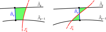
  Figure 34. The polygon $\mathrm{Pol}(q)$ when $q-1$ and $q$ are crossing parameters.

• If $q-1$ is a crossing parameter and $q$ is a U-turn, then there are four cases to consider, depending on whether $J_{k}^{i}$ intersects $\tilde{B}_{q}$ or not, and whether it first intersects $\tilde{B}_{q+1}$ or $\tilde{\beta}_{q+1}$. See Figure 35.

  

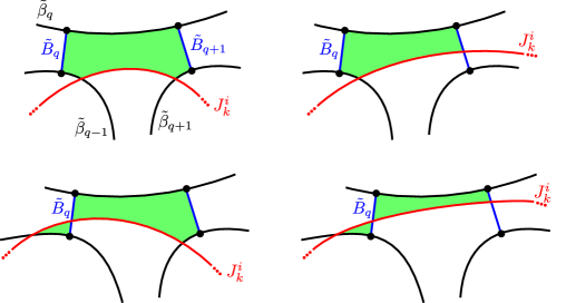
  Figure 35. The polygon $\mathrm{Pol}(q)$ in the mixed case.

• The symmetric case, when $q-1$ is a U-turn parameter and $q$ a crossing parameter.

• In the case when both $q-1$ and $1$ are U-turn parameters, there are also four cases to consider, depending on whether $J_{k}^{i}$ first intersects $\tilde{\beta}_{q-2}$ or $\tilde{B}_{q-1}$, and $\tilde{\beta}_{q+1}$ or $\tilde{B}_{q+1}$. See Figure 36.

  

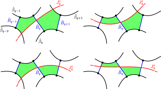
  Figure 36. The polygon $\mathrm{Pol}(q)$ when $q-1$ and $q$ are U-turn parameters.

∎

Remark 10.8.

In the case the junction $J_{k}^{i}$ intersects the bar $\tilde{B}_{q}$, the polygon $\mathrm{Pol}(q)$ is not convex but rather made of two disjoint true polygons $\mathrm{Pol}(q)=\mathrm{Pol}^{1}(q)\sqcup\mathrm{Pol}^{2}(q)$, one at the left of the bar $\tilde{B}_{q}$, the other one at its right. It can also happen that the polygon $\mathrm{Pol}(q)$ is degenerate, which happens if and only if the junction $J_{k}^{i}$ coincides with the bar $\tilde{B}_{q}$.

Because of the presence of these contractible polygons $\mathrm{Pol}(q)$, all the bars $\tilde{B}_{q}$ (or their projections $\overline{B}_{q}$ to $\mathbf{S}$), for $q\in\{\psi_{k}^{i}+1,...,\psi_{k+1}^{i}\}$, are said to be superseded by the polygon $\mathrm{Pol}(q)$. Each bar in the family $\overline{B}$ is superseded twice: if $\iota:\Theta\rightarrow\Theta$ is the involution switching signs, then $\overline{B}_{q}$ is superseded by $\mathrm{Pol}(q)$ and $\overline{B}_{\iota q}$ by $\mathrm{Pol}(\iota q)$.

Remark 10.9.

In the special case when $q\in\{\psi_{k}^{i}+1,\ldots,\psi_{k+1}^{i}-1\}$ is a U-turn parameter, then the junction $J_{k}^{i}$ does not intersect $\tilde{\beta}_{q}$, and the entirety of the simple portion $\tilde{\mathcal{I}}_{q}$ is included in the boundary of $\mathrm{Pol}(q)$. We say that $\overline{\mathcal{I}}_{q}$ is shielded by the junction $J_{k}^{i}$: there is a contractible component of $\mathbf{S}\setminus\mathbf{c}^{\mathrm{f}}$ containing $\overline{\mathcal{I}}_{q}$ in its boundary.

10.2. Upper bound on $\ell_{Y}(\Gamma_{\lambda})$

The upper bound will be related to neutralizations within the family of polygonal curves $(\Gamma_{\lambda})_{\lambda\in\Lambda}$. We invite the reader to remind themselves of the notations introduced in §8, and in particular the notion of height of a cell $Z^{\mathbf{\Gamma}}_{K}$ from Notation 8.27, the conventions related to simultanous decorations from §8.5.3, and the notion of surviving boundary segment $\mathcal{K}_{q}$, $q\in\Theta_{\mathrm{surv}}$, and associated height $Z_{{\mathbf{\Gamma}},{\mathbf{d}}}(\mathcal{K}_{q})$, introduced in Definition 8.39.

10.2.1. A useful lemma

The following lemma, illustrated in Figure 37, is an obvious consequence of the variational characterization of geodesics and orthogeodesics. Here we use Lemma 8.11, which allows us to compare certain orthogedesics with the height function introduced in Definition 8.5.

Proposition 10.10.

Let $\Gamma=(J_{j},K_{j})_{j\in\mathbb{Z}_{m}}$ be a polygonal curve. Let $I=\{a,\ldots,b\}$ be an interval of $\mathbb{Z}_{m}$ of length $\geq 2$. For $x,y$ be two points in the roof $\tilde{J}_{I}$ over $(K_{i})_{i\in I}$, denote as $\gamma_{xy}$ the subsegment of $\tilde{J}_{I}$ between $x$ and $y$. Let $\gamma=\gamma_{1}\mathord{\mathchoice{\,\vbox{\hbox{\scalebox{0.5}{$\displaystyle\bullet$}}}\,}{\,\vbox{\hbox{\scalebox{0.5}{$\textstyle\bullet$}}}\,}{\,\vbox{\hbox{\scalebox{0.5}{$\scriptstyle\bullet$}}}\,}{\,\vbox{\hbox{\scalebox{0.5}{$\scriptscriptstyle\bullet$}}}\,}}\kappa_{1}\mathord{\mathchoice{\,\vbox{\hbox{\scalebox{0.5}{$\displaystyle\bullet$}}}\,}{\,\vbox{\hbox{\scalebox{0.5}{$\textstyle\bullet$}}}\,}{\,\vbox{\hbox{\scalebox{0.5}{$\scriptstyle\bullet$}}}\,}{\,\vbox{\hbox{\scalebox{0.5}{$\scriptscriptstyle\bullet$}}}\,}}\gamma_{2}\mathord{\mathchoice{\,\vbox{\hbox{\scalebox{0.5}{$\displaystyle\bullet$}}}\,}{\,\vbox{\hbox{\scalebox{0.5}{$\textstyle\bullet$}}}\,}{\,\vbox{\hbox{\scalebox{0.5}{$\scriptstyle\bullet$}}}\,}{\,\vbox{\hbox{\scalebox{0.5}{$\scriptscriptstyle\bullet$}}}\,}}\cdots\mathord{\mathchoice{\,\vbox{\hbox{\scalebox{0.5}{$\displaystyle\bullet$}}}\,}{\,\vbox{\hbox{\scalebox{0.5}{$\textstyle\bullet$}}}\,}{\,\vbox{\hbox{\scalebox{0.5}{$\scriptstyle\bullet$}}}\,}{\,\vbox{\hbox{\scalebox{0.5}{$\scriptscriptstyle\bullet$}}}\,}}\kappa_{n}\mathord{\mathchoice{\,\vbox{\hbox{\scalebox{0.5}{$\displaystyle\bullet$}}}\,}{\,\vbox{\hbox{\scalebox{0.5}{$\textstyle\bullet$}}}\,}{\,\vbox{\hbox{\scalebox{0.5}{$\scriptstyle\bullet$}}}\,}{\,\vbox{\hbox{\scalebox{0.5}{$\scriptscriptstyle\bullet$}}}\,}}\gamma_{n+1}$ (with $n\geq 1$) be a path joining $x$ and $y$, homotopic to $\gamma_{xy}$, such that:

• for $1\leq i\leq n+1$, $\gamma_{i}$ is a piecewise geodesic path;

• for $1\leq i\leq n$, $\kappa_{i}$ is a geodesic segment contained in a segment $K_{m_{i}}$ for a $m_{i}\in I$.

Then, for any arbitrary subset $\pi$ of $\mathbb{Z}_{m}$,

(10.8) $$\ell(\gamma_{xy})\leq\sum_{\begin{subarray}{c}1\leq i\leq n\\ \kappa_{i}\notin\pi\end{subarray}}\ell(\kappa_{i})+\sum_{i=1}^{n+1}\ell(\gamma_{i})+\sum_{j\in I\cap\pi}(\log Z^{\Gamma}_{K_{j}}+2),$$

where $\kappa_{i}\notin\pi$ means that the segment $K_{m_{i}}$ containing $\kappa_{i}$ has index $m_{i}\not\in\pi$.

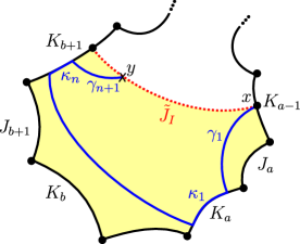
Figure 37. Illustration of the length inequality in a neutralized polygonal curve.

In practice, $\gamma$ will be simple (which implies that the indices $m_{i}$ are monotonically ordered), and the paths $\gamma_{i}$ will not intersect the cells $(K_{j})_{j\in\mathbb{Z}_{m}}$ except at their endpoints.

Remark 10.11.

If $x$ is the origin of $\tilde{J}_{I}$, then we can replace in this upper bound $\gamma_{1}$ by any piecewise geodesic path $\gamma^{\prime}_{1}$, starting anywhere on $K_{a-1}$ and ending at the origin of $\kappa_{1}$. A similar remark holds if $y$ is the endpoint of $\tilde{J}_{I}$ lying in $K_{b+1}$.

The same result also holds with $I=\mathbb{Z}_{m}$, $\tilde{J}_{I}$ replaced by $\Gamma$, and $\gamma=\gamma_{1}\mathord{\mathchoice{\,\vbox{\hbox{\scalebox{0.5}{$\displaystyle\bullet$}}}\,}{\,\vbox{\hbox{\scalebox{0.5}{$\textstyle\bullet$}}}\,}{\,\vbox{\hbox{\scalebox{0.5}{$\scriptstyle\bullet$}}}\,}{\,\vbox{\hbox{\scalebox{0.5}{$\scriptscriptstyle\bullet$}}}\,}}\kappa_{1}\mathord{\mathchoice{\,\vbox{\hbox{\scalebox{0.5}{$\displaystyle\bullet$}}}\,}{\,\vbox{\hbox{\scalebox{0.5}{$\textstyle\bullet$}}}\,}{\,\vbox{\hbox{\scalebox{0.5}{$\scriptstyle\bullet$}}}\,}{\,\vbox{\hbox{\scalebox{0.5}{$\scriptscriptstyle\bullet$}}}\,}}\gamma_{2}\mathord{\mathchoice{\,\vbox{\hbox{\scalebox{0.5}{$\displaystyle\bullet$}}}\,}{\,\vbox{\hbox{\scalebox{0.5}{$\textstyle\bullet$}}}\,}{\,\vbox{\hbox{\scalebox{0.5}{$\scriptstyle\bullet$}}}\,}{\,\vbox{\hbox{\scalebox{0.5}{$\scriptscriptstyle\bullet$}}}\,}}\cdots\mathord{\mathchoice{\,\vbox{\hbox{\scalebox{0.5}{$\displaystyle\bullet$}}}\,}{\,\vbox{\hbox{\scalebox{0.5}{$\textstyle\bullet$}}}\,}{\,\vbox{\hbox{\scalebox{0.5}{$\scriptstyle\bullet$}}}\,}{\,\vbox{\hbox{\scalebox{0.5}{$\scriptscriptstyle\bullet$}}}\,}}\kappa_{n}$ a piecewise geodesic curve (hence closed), freely homotopic to $\Gamma$ (the only difference being that there is the same number of $\kappa_{i}$ and $\gamma_{i}$, i.e. (10.8) now runs for $1\leq i\leq n$ for both sums).

Proof.

First we observe that, under the hypotheses of the statement, by the variational definition of the geodesic,

(10.9) $$\ell(\gamma_{xy})\leq\sum_{i=1}^{n}\ell(\kappa_{i})+\sum_{i=1}^{n+1}\ell(\gamma_{i}).$$

We then observe that the path $\gamma$ has to intersect each of the segments $W_{j_{i}}$ defined in Definition 8.10. More precisely, there is a portion of $\gamma$ containing $\kappa_{i}$ and homotopic to a portion of $W_{j_{i}}$. Thus, we replace $\gamma$ by a piecewise geodesic path in the same homotopy class, where each segment $\kappa_{i}$ such that $m_{i}\in\pi$ is suppressed and replaced by a portion of $W_{m_{i}}$. The result then follows from the minimizing property of $\gamma_{xy}$ together with Lemma 8.11. ∎

10.2.2. New representants of $\Gamma_{\lambda}$

In the spirit of the previous length inequality, we construct a new representant to each free homotopy class $\Gamma_{\lambda}$, which approximates its length well.

Notation 10.12.

Throughout the rest of this section, we fix an exhaustion $(\mathbf{\Gamma},\mathbf{d})=(\Gamma^{k},d^{k})_{1\leq k\leq t}$ of the family of polygonal curves $\Gamma=(\Gamma_{\lambda})_{\lambda\in\Lambda}$. For $\lambda\in\Lambda$, write

$$\Gamma^{k}_{\lambda}=(J_{j}^{\lambda,k},K_{j}^{\lambda,k})_{j\in\mathbb{Z}_{n_{\lambda}^{k}}}.$$

For $k=t$ the terminal polygonal curve, we simply denote $\Gamma^{\infty}_{\lambda}=(J_{j}^{\lambda},K_{j}^{\lambda})_{j\in\mathbb{Z}_{n_{\lambda}}}$.

Remember that we also fixed a $\xi\in\Xi$ and $\mathcal{Q}\subseteq I(\xi)$, see Notation 10.3.

In the following we focus on the elements $\lambda\in\Lambda_{\mathrm{BC}}^{\Gamma}$, that is to say, boundary curves. Let us call $\gamma_{\lambda}$ the closed geodesic homotopic to $\Gamma^{1}_{\lambda}$. For $k\in\{1,\ldots,t\}$ there exists a closed annular region $\mathrm{A}_{\lambda}^{k}$ bordered, on one side by $\gamma_{\lambda}$, on the other side by the polygonal curve $\Gamma^{k}_{\lambda}$. Note that we have the inclusion $\mathrm{A}_{\lambda}^{k}\subseteq\mathrm{A}_{\lambda}^{k-1}$ for $k\geq 2$.

The following lemma is an immediate consequence of our construction.

Lemma 10.13.

For $k\in\{1,\ldots,t\}$, we can find a simple, piecewise geodesic representative $\tilde{\Gamma}_{\lambda}^{k}$ of the free homotopy class $\Gamma_{\lambda}$, contained in the annulus $\mathrm{A}_{\lambda}^{k}$, written as a cyclic concatenation

(10.10) $$\tilde{\Gamma}_{\lambda}^{k}=\gamma_{1}^{\lambda,k}\mathord{\mathchoice{\,\vbox{\hbox{\scalebox{0.5}{$\displaystyle\bullet$}}}\,}{\,\vbox{\hbox{\scalebox{0.5}{$\textstyle\bullet$}}}\,}{\,\vbox{\hbox{\scalebox{0.5}{$\scriptstyle\bullet$}}}\,}{\,\vbox{\hbox{\scalebox{0.5}{$\scriptscriptstyle\bullet$}}}\,}}\kappa_{1}^{\lambda,k}\mathord{\mathchoice{\,\vbox{\hbox{\scalebox{0.5}{$\displaystyle\bullet$}}}\,}{\,\vbox{\hbox{\scalebox{0.5}{$\textstyle\bullet$}}}\,}{\,\vbox{\hbox{\scalebox{0.5}{$\scriptstyle\bullet$}}}\,}{\,\vbox{\hbox{\scalebox{0.5}{$\scriptscriptstyle\bullet$}}}\,}}\ldots\mathord{\mathchoice{\,\vbox{\hbox{\scalebox{0.5}{$\displaystyle\bullet$}}}\,}{\,\vbox{\hbox{\scalebox{0.5}{$\textstyle\bullet$}}}\,}{\,\vbox{\hbox{\scalebox{0.5}{$\scriptstyle\bullet$}}}\,}{\,\vbox{\hbox{\scalebox{0.5}{$\scriptscriptstyle\bullet$}}}\,}}\gamma^{\lambda,k}_{s_{\lambda}^{k}}\mathord{\mathchoice{\,\vbox{\hbox{\scalebox{0.5}{$\displaystyle\bullet$}}}\,}{\,\vbox{\hbox{\scalebox{0.5}{$\textstyle\bullet$}}}\,}{\,\vbox{\hbox{\scalebox{0.5}{$\scriptstyle\bullet$}}}\,}{\,\vbox{\hbox{\scalebox{0.5}{$\scriptscriptstyle\bullet$}}}\,}}\kappa^{\lambda,k}_{s_{\lambda}^{k}}$$

where:

• $\gamma_{j}^{\lambda,k}$ is piecewise geodesic, made of portions of junctions and bridges of $\Gamma^{k}_{\lambda}$;

• $\kappa_{j}^{\lambda,k}$ is a geodesic segment contained in one of the cells of $\Gamma_{\lambda}^{k}$.

The representative $\tilde{\Gamma}_{\lambda}^{k}$ is unique if we ask that the annulus $\tilde{\mathrm{A}}_{\lambda}^{k}$ bordered by $\gamma_{\lambda}$ and by $\tilde{\Gamma}_{\lambda}^{k}$ does not contain any junction in its interior.

In particular, $\gamma_{j}^{\lambda,k}$ does not intersect the cells of $\Gamma_{\lambda}^{k}$ except at its endpoints.

For $k=t$, we write $\gamma_{j}^{\lambda}=\gamma_{j}^{\lambda,t}$ and $\kappa_{j}^{\lambda}=\kappa_{j}^{\lambda,t}$ for $1\leq j\leq s_{\lambda}=s_{\lambda}^{t}$.

10.2.3. Length inequalities: junctions

We prove the following comparison between the lengths of the paths $(\gamma_{j}^{\lambda,1})_{1\leq j\leq s_{\lambda}^{1}}$ and the total length of all junctions.

Lemma 10.14.

We have that

$$\sum_{\lambda\in\Lambda_{\mathrm{BC}}^{\Gamma}}\sum_{j=1}^{s_{\lambda}^{1}}\ell(\gamma_{j}^{\lambda,1})\leq\sum_{p\in\operatorname{Junc}(\mathcal{Q})}\ell(p).$$

Proof.

We observe that, for $\lambda\in\Lambda_{\mathrm{BC}}^{\Gamma}$, the union of paths $\bigcup_{1\leq j\leq s_{\lambda}^{1}}\gamma_{j}^{\lambda,1}$ is composed of disjoint subsegments of junctions, that we call $(j_{l}^{\lambda})_{1\leq l\leq M_{\lambda}}$, and subsegments of the bridges of $\Gamma^{1}$, which we denote as $(b_{l}^{\lambda})_{1\leq l\leq m_{\lambda}}$. Since the bridges of $\Gamma^{1}$ are bars $\overline{B}_{q}$, the paths $(b_{l}^{\lambda})_{1\leq l\leq m_{\lambda}}$ are subsegments of bars.

We claim that to each segment $b_{l}^{\lambda}$ we can associate a subset $P(b_{l}^{\lambda})$ satisfying the following properties:

• $P(b_{l}^{\lambda})$ is included in $\bigcup_{p\in\operatorname{Junc}(\mathcal{Q})}p$ and disjoint from all $(j^{\lambda^{\prime}}_{l^{\prime}})_{\lambda^{\prime},1\leq l^{\prime}\leq M_{\lambda^{\prime}}}$;

• $\ell(b_{l}^{\lambda})\leq\ell(P(b_{l}^{\lambda}))$;

• the $P(b_{l}^{\lambda})$ are mutually disjoint for distinct $(l,\lambda)$.

Indeed, $b_{l}^{\lambda}$ is included in the bar $\overline{B}_{q}$ for an index $q$. This means that $b_{l}^{\lambda}$ is one of the boundary segments of the polygon $\mathrm{Pol}(q)\cup\mathrm{Pol}(\iota q)$. The two polygons $\mathrm{Pol}(q)$ and $\mathrm{Pol}(\iota q)$ share a side, namely $\overline{B}_{q}$. Because their union still contains the subset $b_{l}^{\lambda}$ of $\overline{B}_{q}$ in its boundary, their intersection $\mathrm{Pol}(q)\cap\mathrm{Pol}(\iota q)$ must be a polygon, the boundary of which consists of the union of:

• the entire segment $b_{l}^{\lambda}$ itself;

• a subset of $\bigcup_{p\in\operatorname{Junc}(\mathcal{Q})}p$ made of pieces of boundary of $\mathrm{Pol}(q)$ in the interior of $\mathrm{Pol}(\iota q)$, or pieces of boundary of $\mathrm{Pol}(\iota q)$ in the interior of $\mathrm{Pol}(q)$;

• and, perharps, some pieces of $\beta_{\lambda(q)}$ or $\beta_{\lambda(q-1)}$, orthogonal to $b_{l}^{\lambda}$.

We define $P(b_{l}^{\lambda})$ to be the set of points in the boundary of $\mathrm{Pol}(q)\cap\mathrm{Pol}(\iota q)$ which belong in $\bigcup_{p\in\operatorname{Junc}(\mathcal{Q})}p$. By an enumuration of all cases, a few of which are illustrated in Figure 38, we check that this set satisfies the length inequality, using either the variational characterization of geodesics or orthogeodesics.

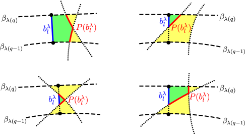
Figure 38. The construction of $P(b_{l}^{\lambda})$ in all cases where $q$ and $\iota(q)$ are crossing parameters. The overall shaded area is the union of $\mathrm{Pol}(q)$ and $\mathrm{Pol}(\iota(q))$, with the intersection represented in green. The dotted lines are the irrelevant portions of the junctions and bars, and the dashed lines the multi-curve $\beta$.

We can then write

$$\sum_{\lambda\in\Lambda_{\mathrm{BC}}^{\Gamma}}\sum_{j=1}^{s_{\lambda}^{1}}\ell(\gamma_{j}^{\lambda,1}) =\sum_{\begin{subarray}{c}\lambda\in\Lambda_{\mathrm{BC}}^{\Gamma}\\ 1\leq l\leq M_{\lambda}\end{subarray}}\ell(j^{\lambda}_{l})+\sum_{\begin{subarray}{c}\lambda\in\Lambda_{\mathrm{BC}}^{\Gamma}\\ 1\leq l\leq m_{\lambda}\end{subarray}}\ell(b_{l}^{\lambda})$$

$$\leq\ell\Big{(}\bigsqcup_{\begin{subarray}{c}\lambda\in\Lambda_{\mathrm{BC}}^{\Gamma}\\ 1\leq l\leq M_{\lambda}\end{subarray}}j_{l}^{\lambda}\sqcup\bigsqcup_{\begin{subarray}{c}\lambda\in\Lambda_{\mathrm{BC}}^{\Gamma}\\ 1\leq l\leq m_{\lambda}\end{subarray}}P(b_{l}^{\lambda})\Big{)}\leq\sum_{p\in\operatorname{Junc}(\mathcal{Q})}\ell(p)$$

because the $j^{\lambda}_{l}$ and $P(b_{l}^{\lambda})$ are disjoint subsegments of the set of junctions. ∎

10.2.4. Length inequalities and double points

Let us now prove some length inequalities related to the portions of cells $(\kappa_{j}^{\lambda})_{\lambda,j}$. We observe that the sets $(\beta_{\lambda})_{\lambda\in\Lambda_{\mathrm{BC}}^{\beta}}$ and $(\kappa_{j}^{\lambda})_{\lambda\in\Lambda_{\mathrm{BC}}^{\Gamma},1\leq j\leq s_{\lambda}}$ are included in $\beta$, and that each point of $\beta$ belongs to at most two of them. In particular,

(10.11) $$\sum_{\lambda\in\Lambda_{\mathrm{BC}}^{\beta}}\ell_{Y}(\beta_{\lambda})+\sum_{\lambda\in\Lambda_{\mathrm{BC}}^{\Gamma}}\sum_{1\leq j\leq s_{\lambda}}\ell(\kappa_{j}^{\lambda})\leq 2\ell_{Y}(\beta).$$

This is also true if we restrict the left-hand-side to smaller sets.

Notation 10.15.

In the rest of this section, we shall consider arbitrary subsets $V^{\Gamma}\subseteq\Lambda_{\mathrm{BC}}^{\Gamma}$, $V^{\beta}\subseteq\Lambda_{\mathrm{BC}}^{\beta}$, $\pi\subseteq\Theta_{\mathrm{surv}}$. We let $V=V^{\beta}\sqcup V^{\Gamma}$. We write $\kappa_{j}^{\lambda}\notin\pi$ iff the cell containing $\kappa_{j}^{\lambda}$ is not in $\pi$. We denote $\Theta_{\tau}(\pi):=\bigcup_{q\in\pi}\Theta_{\tau}(q)$ the set of indices corresponding to the segments $\mathcal{K}_{q}$ that are in $\pi$.

Plugging in these subsets, (10.11) directly implies

(10.12) $$\sum_{\lambda\in V^{\beta}}\ell_{Y}(\beta_{\lambda})+\sum_{\lambda\in V^{\Gamma}}\sum_{\begin{subarray}{c}1\leq j\leq s_{\lambda}\\ \kappa_{j}^{\lambda}\notin\pi\end{subarray}}\ell(\kappa_{j}^{\lambda})\leq 2\ell_{Y}(\beta).$$

The aim of this subsection is to improve this inequality by determining the points which are counted twice.

Definition 10.16.

We call a point in $\beta$ simple if it satisfies either of these conditions:

• it belongs to $\bigcup_{\lambda\in\Lambda_{\mathrm{in}}^{\beta}}\beta_{\lambda}$ and to at most one interval $\kappa_{j}^{\lambda}$ with $\lambda\in V^{\Gamma}$ and $\kappa_{j}^{\lambda}\notin\pi$;

• it belongs to $\bigcup_{\lambda\in V^{\beta}}\beta_{\lambda}$ and to none of the intervals $\kappa_{j}^{\lambda}$ with $\lambda\in V^{\Gamma}$ and $\kappa_{j}^{\lambda}\notin\pi$;

• or it belongs to $\bigcup_{\lambda\in\Lambda_{\mathrm{BC}}^{\beta}\setminus V^{\beta}}\beta_{\lambda}$.

Other points are called double. We call $D$ the set of double points.

Obviously, if $|D|$ stands for the 1-dimensional Lebesgue measure of $D$ as a subset of $\beta$,

(10.13) $$\sum_{\lambda\in V^{\beta}}\ell_{Y}(\beta_{\lambda})+\sum_{\lambda\in V^{\Gamma}}\sum_{\begin{subarray}{c}1\leq j\leq s_{\lambda}\\ \kappa_{j}^{\lambda}\notin\pi\end{subarray}}\ell(\kappa_{j}^{\lambda})\leq\ell_{Y}(\beta)+|D|.$$

We now prove a bound on $|D|$.

Proposition 10.17.

We have that

$$|D|\leq\sum_{\begin{subarray}{c}q\in\mathcal{Q}\cap\Theta_{\ell}(V)\\ q\notin\Theta_{\tau}(\pi)\end{subarray}}\tilde{\theta}_{q}.$$

The proof essentially revolves around the following lemma.

Lemma 10.18.

All the following points are simple:

• points in $\mathcal{K}_{q}$ where $\mathcal{K}_{q}$ is a cell of $\Gamma_{\lambda}$ with $\lambda\notin V^{\Gamma}$ or $\kappa_{l}^{\lambda}\in\pi$;

• points in $\bigcup_{\lambda\notin V^{\beta}}\beta_{\lambda}$;

• for $q\in I(\xi)$, points in $\overline{\mathcal{I}}_{q}\setminus[G_{q},D_{q}]$;

• points in $\overline{\mathcal{I}}_{q}$ where $q\not\in I(\xi)$;

• for $q\in I(\xi)\setminus\mathcal{Q}$, all points in $\overline{\mathcal{I}}_{q}$;

Proof of Lemma 10.18.

Items (a), (a’) are obvious.

Item (b) is also straightforward, because there are two junctions arriving at $G_{q}$ and $D_{q}$, which are responsible for the points in $\overline{\mathcal{I}}_{q}\setminus[G_{q},D_{q}]$ being simple.

For item (c), if $q\not\in I(\xi)$ then there is a junction that crosses $\beta_{\lambda(q)}$ transversally, say at a point $x_{q}$, which is a vertex both of $\mathrm{Pol}(q)$ and of $\mathrm{Pol}(q+1)$. The two intervals $[x_{q},o(\overline{\mathcal{I}}_{q+1})]$ and $[x_{q},t(\overline{\mathcal{I}}_{q})]$ consist of simple points (see Figure 39), and their union contains $\overline{\mathcal{I}}_{q}$.

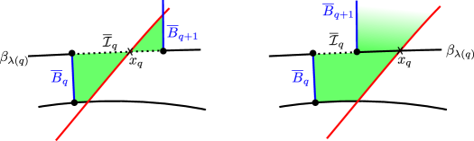
Figure 39. Illustration of case (c) in the proof of Lemma 10.18. The two highlighted polygonals are $\mathrm{Pol}(q)$ and $\mathrm{Pol}(q+1)$. The dashed path is $\overline{\mathcal{I}}_{q}$.

Regarding item (d), if $q\in(I(\xi)\setminus\mathcal{Q})\cap\mathcal{C}$, there is again a junction that crosses $\beta_{\lambda(q)}$ transversally, and we can argue as for Item (c). If $q\in(I(\xi)\setminus\mathcal{Q})\cap\mathcal{U}$ we use Remark 10.9, showing that the points in $\overline{\mathcal{I}}_{q}$ are simple. ∎

Proof of Proposition 10.17.

We write $\beta=\bigcup_{q\in\Theta}\overline{\mathcal{I}}_{q}$, where the geodesic segments are just defined as subsets of $\beta$, that is to say, we forget about their orientations. These intervals may overlap: this is the case if some of the $\theta_{q}$ were negative, or were positive but very large. By Lemma 10.18, the only possibly double points are contained in segments $[G_{q},D_{q}]$ where $q\in\mathcal{Q}\cap\Theta_{\ell}(V)$ with $q\notin\Theta_{\tau}(\pi)$. This implies the claim if we recall that $\tilde{\theta}_{q}$ is the length of $[G_{q},D_{q}]$. ∎

10.2.5. The upper bound

We are now ready to state and prove our upper bound.

Proposition 10.19.

Let $\xi\in\Xi$, $\mathcal{Q}\subseteq I(\xi)$, and $(\mathbf{\Gamma},\mathbf{d})$ be an exhaustion of $(\Gamma_{\lambda})_{\lambda\in\Lambda}$. For any arbitrary sets $V\subseteq\Lambda_{\mathrm{BC}}$ and $\pi\subseteq\Theta_{\mathrm{surv}}$, on the support of $\Psi_{\mathbf{\Gamma},\mathbf{d}}$, we have

$$\sum_{\lambda\in V}\ell_{Y}(\Gamma_{\lambda})\leq\ell_{Y}({\mathbf{c}})+\sum_{\begin{subarray}{c}q\in\mathcal{Q}\cap\Theta_{\ell}(V)\\ q\notin\Theta_{\tau}(\pi)\end{subarray}}\tilde{\theta}_{q}+\sum_{q\in\pi}(\log Z_{\mathbf{\Gamma},\mathbf{d}}(\mathcal{K}_{q})+2)+\mathrm{fn}(r)$$

where $\Theta_{\tau}(\pi)=\bigcup_{q\in\pi}\Theta_{\tau}(q)$.

Proof.

Denote $V^{\beta}=V\cap\Lambda^{\beta}$ and $V^{\Gamma}=V\cap\Lambda^{\Gamma}$. For $\lambda\in\Lambda_{\mathrm{BC}}^{\Gamma}$ and $k\in\{1,\ldots,t-1\}$, we define

$$\mathcal{S}_{\lambda}^{k}=\{K\in\operatorname{Cell}(\Gamma_{\lambda}^{k}):\exists K^{\prime}\in\operatorname{Cell}(\Gamma^{k+1}),K^{\prime}\subseteq K\},$$

the set of cells of $\Gamma_{\lambda}^{k}$ that “survive” at step $k+1$ of the exhaustion. Denote $\mathcal{Z}_{\lambda}^{k}=\operatorname{Cell}(\Gamma_{\lambda}^{k})\setminus\mathcal{S}_{\lambda}^{k}$ the set of cells of $\Gamma_{\lambda}^{k}$ that are neutralized at step $k+1$. By repeated application of Proposition 10.10, we obtain that, for any $Y$ in the support of $\Psi_{\mathbf{\Gamma},\mathbf{d}}$,

$$\ell_{Y}(\Gamma_{\lambda})=\ell(\gamma_{\lambda})\leq\sum_{j=1}^{s_{\lambda}}\ell(\gamma_{j}^{\lambda})+\sum_{\begin{subarray}{c}1\leq j\leq s_{\lambda}\\ \kappa_{j}^{\lambda}\notin\pi\end{subarray}}\ell(\kappa_{j}^{\lambda})+\sum_{q\in\pi\cap\Theta_{\ell}(\lambda)}(\log Z_{\mathbf{\Gamma},\mathbf{d}}(\mathcal{K}_{q})+2)$$

and, for $k\in\{2,\ldots,t\}$,

$$\sum_{j=1}^{s_{\lambda}^{k}}\ell(\gamma_{j}^{\lambda,k})\leq\sum_{j=1}^{s_{\lambda}^{k-1}}\ell(\gamma_{j}^{\lambda,k-1})+\sum_{K\in\mathcal{Z}_{\lambda}^{k-1}}(\log Z^{\mathbf{\Gamma}}_{K}+2).$$

Put together, this yields

$$\ell_{Y}(\Gamma_{\lambda})\leq\sum_{j=1}^{s_{\lambda}^{1}}\ell(\gamma_{j}^{\lambda,1})+\sum_{\begin{subarray}{c}1\leq j\leq s_{\lambda}\\ \kappa_{j}^{\lambda}\notin\pi\end{subarray}}\ell(\kappa_{j}^{\lambda})+\sum_{q\in\pi\cap\Theta_{\ell}(\lambda)}(\log Z_{{\mathbf{\Gamma}},{\mathbf{d}}}(\mathcal{K}_{q})+2)+\sum_{k=1}^{t-1}\sum_{K\in\mathcal{Z}_{\lambda}^{k}}(\log Z^{\mathbf{\Gamma}}_{K}+2).$$

Let us now use the decoration to further estimate this length. If $k\leq t-1$, then for any cell $K\in\mathcal{Z}_{\lambda}^{k}$, there is a cell $K^{\prime}$ of $\Gamma^{k}$, containing $K$, and bearing the decoration $0$ for the exhaustion $(\mathbf{\Gamma},\mathbf{d})$. As a result, by definition of the test function $\Psi_{\mathbf{\Gamma},\mathbf{d}}$, on its support, we have $\log Z^{\mathbf{\Gamma}}_{K^{\prime}}\leq a+1$. Proposition 8.28 then implies $\log Z^{\mathbf{\Gamma}}_{K}\leq a+3$. We can then deduce from the previous bound, after summation over $\lambda\in V^{\Gamma}$, that

$$\sum_{\lambda\in V^{\Gamma}}\ell_{Y}(\Gamma_{\lambda})\leq\sum_{\begin{subarray}{c}\lambda\in V^{\Gamma}\\ 1\leq j\leq s_{\lambda}^{1}\end{subarray}}\ell(\gamma_{j}^{\lambda,1})+\sum_{\lambda\in V^{\Gamma}}\sum_{\begin{subarray}{c}1\leq j\leq s_{\lambda}\\ \kappa_{j}^{\lambda}\notin\pi\end{subarray}}\ell(\kappa_{j}^{\lambda})+\sum_{q\in\pi}(\log Z_{\mathbf{\Gamma},\mathbf{d}}(\mathcal{K}_{q})+2)+\sum_{\begin{subarray}{c}1\leq k\leq t-1\\ \lambda\in V^{\Gamma}\\ K\in\mathcal{Z}_{\lambda}^{k}\end{subarray}}(a+9).$$

In the last sum, the number of terms in the triple sum $\sum_{k=1}^{t-1}\sum_{\lambda\in V^{\Gamma}}\sum_{K\in\mathcal{Z}_{\lambda}^{k}}$ is less than the total number of cells of all $\Gamma_{\lambda}$ with $\lambda\in V^{\Gamma}$; this is less than $4r$.

We now use Lemma 10.14, equation (10.13) and Proposition 10.17 to bound the sum over $\gamma_{j}^{\lambda}$ and $\kappa_{j}^{\lambda}$. We obtain that

$$\sum_{\lambda\in V}\ell_{Y}(\Gamma_{\lambda})=\sum_{\lambda\in V^{\Gamma}}\ell_{Y}(\Gamma_{\lambda})+\sum_{\lambda\in V^{\beta}}\ell_{Y}(\beta_{\lambda})$$

$$\leq\sum_{p\in\operatorname{Junc}(\mathcal{Q})}\ell(p)+\sum_{\lambda\in\Lambda^{\beta}}\ell_{Y}(\beta_{\lambda})+\sum_{\begin{subarray}{c}q\in\mathcal{Q}\cap\Theta_{\ell}(V)\\ q\notin\Theta_{\tau}(\pi)\end{subarray}}\tilde{\theta}_{q}+\sum_{q\in\pi}(\log Z_{\mathbf{\Gamma},\mathbf{d}}(\mathcal{K}_{q})+2)+\mathrm{fn}(r).$$

To conclude, we use the lower bound proven at the beginning of this section, (10.6). ∎

11. Arbitrary loop topologies

We now indicate how to prove Theorem 1.23 when the multi-loop ${\mathbf{c}}$ is not a generalized eight. In this case, the representatives of the homotopy class of ${\mathbf{c}}$ in minimal position may not be isotopic to one another. We choose arbitrarily one such representative – for instance, by putting an auxiliary hyperbolic metric on ${\mathbf{S}}$ and choosing the geodesic representative of ${\mathbf{c}}$ (possibly perturbing it to get rid of multiple intersections).

Let us denote by $\mathcal{N}\subseteq\mathbf{S}$ a regular neighbourhood of ${\mathbf{c}}$. The pair $(\mathcal{N},{\mathbf{c}})$ is a generalized eight, and we may apply the construction of the pairs of pants decomposition of §3.2. We keep the same notation $(\Gamma_{\lambda})_{\lambda\in\Lambda}$ for the pair of pants decomposition of $\mathcal{N}$, with the indices $\Lambda_{\mathrm{BC}}=\Lambda_{\mathrm{BC}}^{\beta}\sqcup\Lambda_{\mathrm{BC}}^{\Gamma}$ corresponding to the boundary components of $\mathcal{N}$, split into the ones which are, or not, components of the simple multi-loop $\beta$.

In $\mathbf{S}$, some of the curves $(\Gamma_{\lambda})_{\lambda\in\Lambda_{\mathrm{BC}}}$ may be contractible. Proposition 1.30 tells us that the existence of contractible $\beta_{\lambda}$ and $\Gamma_{\lambda}$ should help to prove Theorem 1.23, by making comparison estimates easier. On the other hand, contractible boundary components cause two new difficulties.

• While it is relatively easy to enumerate topological types of generalized eights, it seems daunting to make a list of all topological types of multi-loops. We sidestep this difficulty by only ever working with a fixed topological type, in this article. In the applications to spectral gaps of random hyperbolic surfaces [4], the discussion involves all possible topological types appearing in the Selberg trace formula, but we condition the Weil–Petersson measure on the set of tangle-free surfaces, in order to drastically reduce the number of local topological types to consider.

• When we vary the metric $Y$ on $\mathbf{S}$ and consider the piecewise geodesic representative of $\mathbf{c}$, as done in §4.2.1, the orthogeodesics $(\overline{B}_{q})_{q\in\Theta}$ may be ill-defined. This happens if $B_{q}$ is a problematic bar in the sense of Definition 11.4.

11.1. Diagrams and the reconstitution procedure

We recall the notion of diagram $\mathbf{D}$ representing the multi-loop $\mathbf{c}$ introduced in Definition 2.19. A diagram is the data of the simple multi-loop $\beta$ and the bars $B=(B_{1},\ldots,B_{r})$.

11.1.1. Simple portions of diagrams

We extend the notions of simple portions, introduced in Definition 1.21 for multi-loops, to diagrams as follows: a simple portion of $\mathbf{D}$ is a maximal subsegment of $\beta$ that does not meet the endpoints of the bars $B$. These simple portions may be shielded or unshielded, following once again Definition 1.21. The (un)shielded simple portion of ${\mathbf{c}}$ are in natural bijection with (un)shielded simple portion of $\mathbf{D}$.

We do not apply this terminology to the bars $B_{k}$, because they do not play the same role as the curves $\beta_{i}$: indeed, when we describe the isotopy class of $\mathbf{c}$ by following its diagram, all the bars are traversed twice, whilst each simple portion of $\beta$ only once.

11.1.2. Reconstitution procedure

Given a diagram $\mathbf{D}=(\beta,B)$, we may reconstitute a multi-loop $\mathbf{c}$ stemming from $\mathbf{D}$ by the following procedure, guided by the orientation rules in §2.2.2.

The endpoints of the bars cut $\beta$ into $2r$ non-oriented segments $\mathcal{I}_{j}$. Pick a starting segment $\mathcal{I}_{j_{0}}$ and pick arbitrarily one of the two possible orientations of this segment. There a unique closed path starting with $\mathcal{I}_{j_{0}}$, obtained by concatenating alternatively bars $B_{k}$ and segments $\mathcal{I}_{j}$, and respecting the orientation rules. If this path goes through all segments $\mathcal{I}_{j}$, then we obtain a loop (with one component) stemming from $\mathbf{D}$. If not, select another segment $\mathcal{I}_{j}$ that has not been traversed yet, and repeat the procedure until exhaustion of all segments $\mathcal{I}_{j}$.

Starting from a diagram $\mathbf{D}$ with $r$ bars, and letting $\Theta_{\mathbf{D}}:=\{1,\ldots,r\}\times\{\pm\}$, applying the reconstitution procedure gives us an orientation of each segment $\mathcal{I}_{j}$ and their labelling by elements of $\Theta_{\mathbf{D}}$, as well as two oriented copies $(B_{1}^{\pm},\ldots,B_{r}^{\pm})$ of each bar, labelled by $\Theta_{\mathbf{D}}$.

If we start with a multi-loop $\mathbf{c}$ and obtain a diagram $\mathbf{D}$ by opening the intersections (either way), the reconstitution procedure will give us back a multi-loop isotopic to $\mathbf{c}$ (modulo orientation of each component).

The reader may check that a different choice of the original orientation of $\mathcal{I}_{j_{0}}$ will just reverse the orientation of the corresponding component of $\mathbf{c}$. This means that if a multi-loop stemming from $\mathbf{D}$ has $\mathfrak{n}$ components, then the reconstitution procedure can lead to $2^{\mathfrak{n}}$ multi-loops stemming from $\mathbf{D}$, all having the same geometric image, and differing only by orientation of each component.

It seems difficult to determine when two diagrams lead to homotopic multi-loops; we do not address this problem in this paper. In the case of generalized eights, this problem does not occur and we can state the following:

Remark 11.1.

Let $\mathbf{D}$ be a diagram. Assume that ${\mathbf{S}}\setminus\mathbf{D}$ has no connected component which is a disk. Then a multi-loop stemming from $\mathbf{D}$ is a generalized eight and, as a consequence, $\mathbf{D}$ represents a generalized eight; all generalized eights leading to the diagram $\mathbf{D}$ are isotopic (modulo orientation of each component).

Note that each component of a multi-loop $\mathbf{c}$ obtained by the reconstitution procedure may be written by a concatenation such as the one we have obtained in §2.5.1, see (2.6).

11.1.3. Extended diagrams

We can extend the notation of diagram, discarding the condition that the bars do not self-intersect:

Definition 11.2.

An extended diagram $\mathbf{D}$ in $\mathbf{S}$ is the data (modulo isotopy) of a collection of simple disjoint loops $\beta$, and of a collection of bars $B=(B_{1},\ldots,B_{r})$, defined as closed segments with distinct endpoints lying in $\beta$, and disjoint from $\beta$ otherwise.

The reconstitution procedure of §11.1.2 also applies to an extended diagram $\mathbf{D}$. Simple portions of an extended diagram are defined as for usual diagrams. A simple portion of $\mathbf{D}$ is said to be shielded (in $\mathbf{S}$) if it lies in the boundary of a contractible component of $\mathbf{S}\setminus\mathbf{D}$.

Definition 11.3.

Let $\mathbf{D}=(\beta,B)$ be an extended diagram in $\mathbf{S}$, and let $\mathbf{c}=(\mathbf{c}_{1},\ldots,\mathbf{c}_{\mathfrak{n}})$ be a multi-loop obtained from $\mathbf{D}$ by the reconstitution procedure. We say that $\mathbf{D}$ satisfies the minimality condition if:

• the components $\mathbf{c}_{i}$ are non-contractible;

• if $\tilde{\mathbf{c}}_{i}$ is a lift of a component of $\mathbf{c}$ in the universal cover of $\mathbf{S}$, then $\tilde{\mathbf{c}}_{i}$ has no self-intersection;

• any two lifts $\tilde{\mathbf{c}}_{i}$, $\tilde{\mathbf{c}}_{j}$ of components of $\mathbf{c}$ in the universal cover of $\mathbf{S}$ can intersect at most once (with the convention that a shared bar counts for 1 intersection point).

Remark that if we start with a multi-loop $\mathbf{c}$ in minimal position, as we always do, then any diagram $\mathbf{D}$ representing it automatically satisfies the minimality condition; so this is a natural condition to ask for.

Definition 11.4.

A bar of an extended diagram is problematic if it satisfies either of the following two conditions:

• one of its endpoints lies on a contractible loop $\beta_{i}$;

• its two endpoints lie on one same loop $\beta_{i}$, and the bar is homotopically trivial with endpoints gliding along $\beta_{i}$.

Definition 11.5.

A bar of an extended diagram is cylindrical if it runs between $\beta_{i}$ and $\beta_{j}$ with $i\not=j$ and $\beta_{i},\beta_{j}$ are non-contractible, in the same homotopy class.

Cylindrical bars count among the non-problematic bars.

Definition 11.6.

An extended diagram $\mathbf{D}$ is said to be good if it has no problematic bar and if it satisfies the minimality condition.

11.2. An auxiliary generalized eight: the skeleton

The forthcoming Proposition 11.13 says that, by opening intersections from a multi-loop ${\mathbf{c}}$, we can create a generalized eight that has length smaller than ${\mathbf{c}}$ for any hyperbolic metric, and still fills ${\mathbf{S}}$ (or a surface obtained by removing cylinders from ${\mathbf{S}}$). Such an auxilliary loop is called a skeleton; simple examples are represented in Figure 40.

11.2.1. Removing one disk

We first prove the following lemma.

Lemma 11.7.

Let $\mathbf{D}$ be a diagram filling ${\mathbf{S}}$. Assume that at least one of the connected components of ${\mathbf{S}}\setminus\mathbf{D}$ is homeomorphic to a disk. Then we can remove one of the bars of $\mathbf{D}$ so that the resulting diagram $\mathbf{D}^{\prime}$ fills a surface ${\mathbf{S}}^{\prime}$ obtained by removing cylinders from $\mathbf{S}$.

We recall that we have defined the ways to remove a bar in a diagram in §2.4. By construction, ${\mathbf{S}}\setminus\mathbf{D}^{\prime}$ has exactly one less embedded disk than ${\mathbf{S}}\setminus\mathbf{D}$ among its connected components.

Proof.

If one of the loops $\beta_{i}$ are contractible, it borders a disk $D_{i}$. We remove a bar $B_{k}$ touching $\beta_{i}$ (and another components $\beta_{j}$) in the second way, to obtain $\mathbf{D}^{\prime}$. The filled surface ${\mathbf{S}}^{\prime}$ has same Euler characteristic as ${\mathbf{S}}$. If $B_{k}$ lies inside $D_{i}$, then $\beta_{j}$ is also contractible and obviously ${\mathbf{S}}^{\prime}={\mathbf{S}}$. Otherwise, the bar $B_{k}$ is outside the disk $D_{i}$. We have ${\mathbf{S}}^{\prime}={\mathbf{S}}$ except in one particular case, which occurs when $\beta_{i}=\beta_{j}$. In this case, ${\mathbf{S}}^{\prime}$ is obtained from ${\mathbf{S}}$ by removing a cylinder.

Assume now that none of the $\beta_{i}$ are contractible. Consider a contractible connected component $D$ of ${\mathbf{S}}\setminus\mathbf{D}$: pick a bar $B_{k}$ in the boundary of this contractible component and remove it the first way. Either ${\mathbf{S}}^{\prime}={\mathbf{S}}$, or ${\mathbf{S}}^{\prime}$ is obtained from ${\mathbf{S}}$ by removing a cylinder (this can only happen if the two sides of $B_{k}$ touch the open disk $D$). ∎

Examples of both cases appearing in this lemma can be found in Figure 40.

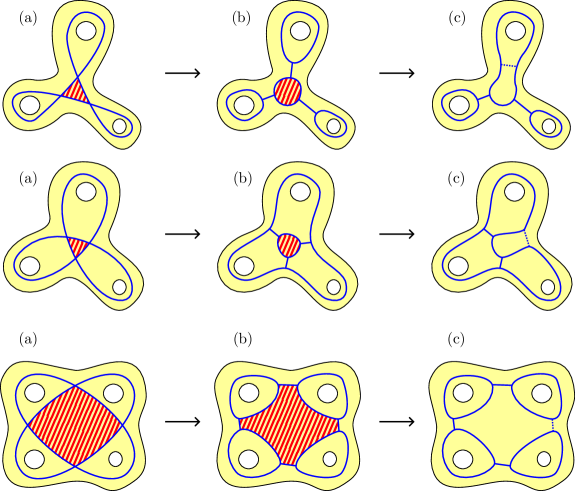
Figure 40. Three examples of (a) loops, (b) diagrams $D^{(1)}$ and (c) skeletons (shown in solid lines). The diagram $D^{(2)}$ is obtained by reincorporating the dashed bar to the skeleton. The two first examples are homotopic, non-isotopic loops.

11.2.2. Skeleton $\mathbf{D}^{\prime}$

By iteration of the process, and using Remark 11.1, we obtain:

Corollary 11.8.

For any diagram $\mathbf{D}$ filling ${\mathbf{S}}$, we can remove bars so that the resulting diagram $\mathbf{D}^{\prime}$ fills a surface ${\mathbf{S}}^{\prime}$ obtained by removing cylinders from $\mathbf{S}$, and so that no connected components of ${\mathbf{S}}^{\prime}\setminus\mathbf{D}^{\prime}$ is contractible. The diagram $\mathbf{D}^{\prime}$ represents a generalized eight ${\mathbf{c}}^{\prime}$.

Definition 11.9.

Let ${\mathbf{c}}$ be a multi-loop with $r$ self-intersections, and $\mathbf{D}^{(1)}=(\beta,B)$ be the diagram obtained by opening all the intersections of ${\mathbf{c}}$ the first way. We call skeleton of ${\mathbf{c}}$ any diagram $\mathbf{D}^{\prime}=(\beta^{\prime},B^{\prime})$ obtained from $\mathbf{D}^{(1)}$ by application of Corollary 11.8. We denote as $r^{\prime}\leq r$ its the number of bars and $\Theta^{\prime}=\{1,\ldots,r^{\prime}\}\times\{\pm\}$. We also refer to the generalized eight ${\mathbf{c}}^{\prime}$ stemming from $\mathbf{D}^{\prime}$, obtained by removing intersections from ${\mathbf{c}}$, as a skeleton of $\mathbf{c}$.

Remark 11.10.

We have $\chi(\mathbf{S})=\chi(\mathbf{S}^{\prime})=r^{\prime}$.

Remark 11.11.

A skeleton is not uniquely defined, because it depends on the order in which we choose the intersection points to remove when iterating Lemma 11.7. It suffices for us to know that a skeleton exists. The forthcoming discussion is completely dependent on the choice of a skeleton.

Remark 11.12.

Even when $\mathbf{S}$ is connected, the surface ${\mathbf{S}}^{\prime}$ may be disconnected, and some connected components may be cylinders containing a component of ${\mathbf{c}}^{\prime}$ which is a simple curve. This happens, in particular, when $\beta_{i}$ and $\beta_{j}^{\pm 1}$ are non-contractible curves bordering a cylinder containing a third curve $\beta_{k}$, in which case $\beta_{k}$ becomes a separate connected component of $\mathbf{S}^{\prime}$ once all its adjacent bars are removed the first way.

Note however that if a bar of $\mathbf{D}$ joins two non-contractible curves $\beta_{i}$, and is not in the boundary of a contractible component of ${\mathbf{S}}\setminus\mathbf{D}$, then this bar stays in each skeleton $\mathbf{D}^{\prime}$. A skeleton $\mathbf{D}^{\prime}$ never contains the cylindrical bars and $\mathbf{S}^{\prime}$ may have more connected components than $\mathbf{S}$, including cylinders (filled by a simple curve).

The multi-curve $\beta^{\prime}$ corresponding to a skeleton ${\mathbf{c}}^{\prime}$ is homotopic to the collection of non-contractible components of $\beta$ in $\mathbf{D}^{(1)}$. In particular, its number of components is smaller.

11.2.3. Length inequality and skeleton

We are now ready to prove our length inequality.

Proposition 11.13.

Let ${\mathbf{c}}$ be a multi-loop in minimal position, filling ${\mathbf{S}}$. Let ${\mathbf{c}}^{\prime}$ be a skeleton of ${\mathbf{c}}$. Then, for any hyperbolic Riemannian metric $Y$ on ${\mathbf{S}}$,

(11.1) $$\ell_{Y}({\mathbf{c}}^{\prime})\leq\ell_{Y}({\mathbf{c}}).$$

The proof relies on the following lemma.

Lemma 11.14.

Let $c_{1}$ and $c_{2}$ be two multi-loops differing by one third Reidemeister move. Let $c_{1}^{\prime}$ be obtained from $c_{1}$ by removing some intersections (in the first or the second way). Then there exists $c^{\prime}_{2}$, homotopic to $c_{1}^{\prime}$, obtained from $c_{2}$ by removing some intersections.

Proof of Lemma 11.14.

This can be checked by simple inspection of a finite number of cases. Two cases are shown in Figure 41.

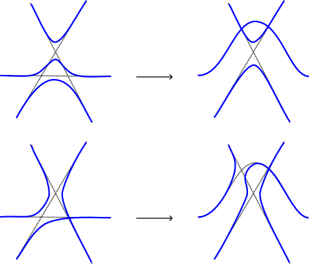
Figure 41. Illustration of two cases arising in the proof of Lemma 11.14.

∎

Proof of Proposition 11.13.

A skeleton ${\mathbf{c}}^{\prime}$ is obtained from ${\mathbf{c}}$ by removing some intersections. Let $Y$ be a hyperbolic Riemannian metric $Y$ on ${\mathbf{S}}$ and $\gamma$ be the geodesic representative of ${\mathbf{c}}$. By definition, $\ell_{Y}({\mathbf{c}})=\ell(\gamma)$. Since $\gamma$ is a geodesic, $\gamma$ is in minimal position: by the results of [7] it is isotopic to ${\mathbf{c}}$ up to a finite number of third Reidemeister moves.

For each Reidemeister move, we shall use Lemma 11.14. We obtain a multi-loop $\gamma^{\prime}$ homotopic to the skeleton ${\mathbf{c}}^{\prime}$, obtained from $\gamma$ by opening some intersections. In the homotopy class of $\gamma^{\prime}$, there is a representative $\gamma_{\varepsilon}$ which just differs from $\gamma$ in an $\varepsilon$-neighbourhood of the intersections (with $\varepsilon>0$ arbitrarily small) and such that $\ell(\gamma_{\varepsilon})<\ell(\gamma)$. More precisely, $\gamma_{\varepsilon}$ may be obtained from local “switchings”, described as follows: take embedded $\varepsilon$-disks $D_{1},\ldots,D_{r}$ around each of the intersection points $a_{1},\ldots,a_{r}$, such that $D_{i}\cap\gamma$ is the union of two simple geodesic segments intersecting once, say $[x_{1},x_{3}]\cup[x_{2},x_{4}]$. The boundary $\partial D_{i}\cap\gamma$ consists of the four cyclically ordered points $x_{1},x_{2},x_{3},x_{4}$, and the multi-loop $\gamma_{\epsilon}$ with removed intersections is such that $D_{i}\cap\gamma_{\epsilon}=[x_{1},x_{2}]\cup[x_{2},x_{3}]$. Outside the disks $D_{i}$, we have $\gamma_{\epsilon}=\gamma$. By the triangle inequality, $\ell([x_{1},x_{2}]\cup[x_{2},x_{3}])<\ell([x_{1},x_{3}]\cup[x_{2},x_{4}])$. Equivalently, $\ell(\gamma_{\varepsilon})<\ell(\gamma)$. To prove the proposition, we combine the two inequalities $\ell_{Y}({\mathbf{c}}^{\prime})\leq\ell(\gamma_{\varepsilon})$, and $\ell(\gamma_{\varepsilon})<\ell(\gamma)=\ell_{Y}({\mathbf{c}})$. ∎

11.3. Good representative of $\mathbf{c}$

The goal of this section is to construct a new representative $\mathbf{D}^{\mathrm{opt}}$ of ${\mathbf{c}}$ which is a good extended diagram: recall that this means a diagram without problematic bars (Definition 11.4) and satisfying the minimality condition (Definition 11.3).

11.3.1. Diagrams $\mathbf{D}^{(2)}$ and $\mathbf{D}^{\prime\prime}$

From the construction of ${\mathbf{c}}^{\prime}$, we see that there exists a diagram $\mathbf{D}^{(2)}$ on $\mathbf{S}$, representing ${\mathbf{c}}$, obtained by:

• gluing to some cylinders to $\mathbf{S}^{\prime}$ to obtain $\mathbf{S}$;

• adding a collection of bars to the diagram $\mathbf{D}^{\prime}$ in $\mathbf{S}$.

Remark 11.15.

The diagram $\mathbf{D}^{(2)}$ is in general different from $\mathbf{D}^{(1)}$, because $\mathbf{D}^{(1)}$ was obtained by opening all intersections the first way, whereas $\mathbf{D}^{(2)}$ is obtained from ${\mathbf{c}}$ by opening the second way certain intersections (running between contractible components of $\beta$).

The added bars may be problematic or non-problematic (cylindrical or not). Since the components of $\beta^{\prime}$ in $\mathbf{D}^{(2)}$ are non-contractible, the problematic bars of $\mathbf{D}^{(2)}$ are only of one kind: they are homotopically trivial bars, running from a component of $\beta^{\prime}$ to itself.

Recall that the (un)shielded simple portions of ${\mathbf{c}}$ are in natural bijection with (un)shielded simple portions of $\mathbf{D}^{(1)}$, and of $\mathbf{D}^{(2)}$. A simple portion of $\mathbf{D}^{\prime}$ can be written as a disjoint union of simple portion of $\mathbf{D}^{(2)}$, only one of which may be unshielded. Since $\mathbf{D}^{\prime}$ is a generalized eight, it has exactly $2\chi(\mathbf{S})$ simple portions. We deduce the following.

Lemma 11.16.

$\mathbf{D}^{(1)}$ and $\mathbf{D}^{(2)}$ have at most $2\chi(\mathbf{S})$ unshielded simple portions.

Definition 11.17.

A simple portion of $\mathbf{D}^{\prime}$ which contains only shielded simple portions of $\mathbf{D}^{(2)}$ will be called a priori neutral.

We introduce a last auxilliary diagram.

Notation 11.18.

Let $\mathbf{D}^{\prime\prime}$ be the diagram obtained by removing from $\mathbf{D}^{(2)}$ its problematic bars.

Lemma 11.19.

$\mathbf{D}^{\prime\prime}$ is a good diagram filling $\mathbf{S}$.

11.3.2. Diagram $\mathbf{D}^{\mathrm{opt}}$

We now prove the following.

Theorem 11.20.

Let $\mathbf{c}$ be a multi-loop in minimal position. Assume that $\mathbf{c}$ is connected and not double-filling. Then there exists good extended diagram $\mathbf{D}^{\mathrm{opt}}$, containing all the non-problematic bars of $\mathbf{D}^{(2)}$, such that $\mathbf{c}$ is homotopic to a multi-loop stemming from $\mathbf{D}^{\mathrm{opt}}$.

Remark 11.21.

We may assume w.l.o.g. that $\mathbf{c}$ is connected. If the surface $\mathbf{S}$ filled by $\mathbf{c}$ is not connected, the previous theorem applies in each connected component of $\mathbf{S}$.

An example of a loop which is not a generalized eight, and a good extended diagram for this loop, is represented in Figure 42.

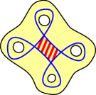
(a) The loop $\mathbf{c}$.

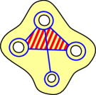
(b) The diagram $\mathbf{D}^{\mathrm{opt}}$.

Figure 42. Example of Theorem 11.20.

Proof.

We prove the result by induction on the total number $n$ of problematic bars of $\mathbf{D}^{(2)}$. The case $n=0$ is obvious as we can take $\mathbf{D}^{\mathrm{opt}}=\mathbf{D}^{(2)}$.

Assume that $n\geq 1$, and that the expected property is known until rank $n-1$. By hypothesis, the diagram $\mathbf{D}^{(2)}$ contains a problematic bar $B_{q}$. Because the bar is problematic regardless of its orientation, we assume w.l.o.g. that $\operatorname{Sign}(q)=+$. By construction of $\mathbf{D}^{(2)}$, the bar $B_{q}$ goes from one component $\beta^{\prime}_{\lambda}$ to itself and is homotopically trivial with gliding endpoints. Denote by $D$ the topological disc bordered by $B_{q}$ and $\beta^{\prime}_{\lambda}$. One of the simple portions adjacent to $B_{q}$ is shielded. To fix ideas, we assume it is $\mathcal{I}_{q}$.

A representative ${\mathbf{c}}^{\mathrm{op}}$ of the homotopy class of $\mathbf{c}$ may be obtained by applying the reconstitution procedure, and allows to write the homotopy class of c as an alternating concatenation of bars and simple portions. Denote $i_{1}=\operatorname{Comp}(q)$ and $i_{2}=\operatorname{Comp}(\iota q)$ so that the bars $B_{q}$ and $B_{\iota q}$ belong to the components ${\mathbf{c}}^{\mathrm{op}}_{i_{1}}$ and ${\mathbf{c}}^{\mathrm{op}}_{i_{2}}$ of ${\mathbf{c}}^{\mathrm{op}}$ respectively.

Recall that $B_{\iota q}$ is the same bar as $B_{q}$ with either the same or the reverse orientation. We treat the case where it has reverse orientation, the other case being similar modulo changes of notation. The local situation near the bar $B_{q}$ is shown on Figure 43.

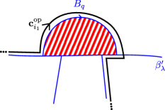
(a) $B_{q}$ and ${\mathbf{c}}^{\mathrm{op}}_{i_{1}}$.

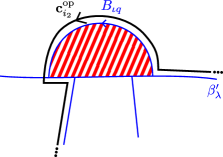
(b) $B_{\iota q}$ and ${\mathbf{c}}^{\mathrm{op}}_{i_{2}}$.

Figure 43. The local situation near the bar $B_{q}$.

We introduce a new surface $\mathbf{S}_{\circ}\subseteq\mathbf{S}$ by taking a regular neighbourhood $\mathcal{N}$ of $\mathbf{D}^{(2)}$ in $\mathbf{S}$ and gluing to $\mathcal{N}$ all connected components of $\mathbf{S}\setminus\mathbf{D}^{(2)}$ that are contractible, except the connected component contained in the disc $D$ and touching the bar $B_{q}$.

In the diagram $\mathbf{D}^{(2)}$, now viewed as a diagram on $\mathbf{S}_{\circ}$, the bar $B_{q}$ is non-problematic. We can therefore apply the induction hypothesis at rank $n-1$ to the multi-loop $\mathbf{c}$ on $\mathbf{S}_{\circ}$. We obtain a good extended diagram $\mathbf{D}^{\mathrm{opt}}_{\circ}$ on $\mathbf{S}_{\circ}$, containing all non-problematic bars of $(\mathbf{S}_{\circ},\mathbf{D}^{(2)})$ (and in particular $B_{q}$), and such that $\mathbf{c}$ is homotopic on $\mathbf{S}_{\circ}$ to a multi-loop stemming from $\mathbf{D}^{\mathrm{opt}}_{\circ}$.

In $\mathbf{S}_{\circ}$ the diagram $\mathbf{D}^{\mathrm{opt}}_{\circ}$ is good, and in $\mathbf{S}$ it has exactly one problematic bar, namely $B_{q}$. We shall define the desired diagram $\mathbf{D}^{\mathrm{opt}}$ by replacing $B_{q}$ by a new non-problematic bar $B_{\mathrm{new}}$.

Applying the reconstitution procedure to $\mathbf{D}^{\mathrm{opt}}_{\circ}$, for each $1\leq i\leq\mathfrak{n}$, we obtain a representative $\mathbf{c}_{i}^{\circ}$ of the homotopy class of ${\mathbf{c}}_{i}$ as a concatenation of bars and simple portions of $\mathbf{D}^{\mathrm{opt}}_{\circ}$. The construction will consist in replacing the two components ${\mathbf{c}}^{\circ}_{i_{1}}$ and ${\mathbf{c}}^{\circ}_{i_{2}}$, containing $B_{q}$ and $B_{\iota q}$ respectively, by new representatives ${\mathbf{c}}^{\mathrm{opt}}_{i_{1}}$ and ${\mathbf{c}}^{\mathrm{opt}}_{i_{2}}$. The other components $({\mathbf{c}}^{\circ}_{i})_{i\neq i_{1},i_{2}}$ will stay untouched.

Lifting the situation to the hyperbolic plane, for $l\in\{1,2\}$, we can write the lift $\tilde{\mathbf{c}}_{i_{l}}^{\circ}$ of $\mathbf{c}_{i_{l}}^{\circ}$ as an infinite concatenation $\mathord{\mathchoice{\,\vbox{\hbox{\scalebox{0.5}{$\displaystyle\bullet$}}}\,}{\,\vbox{\hbox{\scalebox{0.5}{$\textstyle\bullet$}}}\,}{\,\vbox{\hbox{\scalebox{0.5}{$\scriptstyle\bullet$}}}\,}{\,\vbox{\hbox{\scalebox{0.5}{$\scriptscriptstyle\bullet$}}}\,}}_{k\in\mathbb{Z}}\tilde{p}_{k}^{l}$ where, for each $k$, $\tilde{p}_{k}^{l}$ is the concatenation of lifts $\tilde{B}_{k}^{l}$ and $\tilde{\mathcal{I}}_{k}^{l}$ of a bar and a simple portion of $\mathbf{D}^{\mathrm{opt}}_{\circ}$. We pick the indices so that $\tilde{p}^{1}_{0}$ and and $\tilde{p}_{0}^{2}$ contain a lift of $B_{q}$ and $B_{\iota q}$ respectively.

Denote by $\tilde{\beta}_{k}^{l}$ the complete geodesic on $\mathbb{H}^{2}$ containing $\tilde{\mathcal{I}}^{l}_{k}$. We have $\tilde{\beta}_{0}^{1}=\tilde{\beta}_{0}^{2}$ and we call $m>0$ the smallest integer such that $\tilde{\beta}_{m}^{1}\not=\tilde{\beta}_{m}^{2}$. By the minimality condition for ${\mathbf{D}}^{\mathrm{opt}}_{\circ}$, all $k\in\{0,\ldots,m-1\}$ are crossing indices. We define the bar $\tilde{B}_{\mathrm{new}}$ on $\mathbb{H}^{2}$ as the segment going from $t(\tilde{B}^{1}_{m})$ to $t(\tilde{B}^{2}_{m})$, and let $B_{\mathrm{new}}$ be its projection to $\mathbf{S}$. See Figure 44. The desired diagram $\mathbf{D}^{\mathrm{opt}}$ is defined from $\mathbf{D}^{\mathrm{opt}}_{\circ}$ by removing $B_{q}$ and adding the non-problematic bar $B_{\mathrm{new}}$.

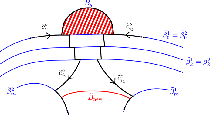
Figure 44. The new bar $B_{\mathrm{new}}$ replacing $B_{q}$.

∎

Remark 11.22.

At each induction step the number of unshielded simple portions of $\mathbf{D}^{\mathrm{opt}}$ in $\mathbf{S}$ stays the same as for the original $\mathbf{D}^{(2)}$, hence it is smaller that $2\chi(\mathbf{S})$.

11.4. Sketch of proof for general topologies

We now explain how to prove Theorem 1.23 for general multi-loops $\mathbf{c}$.

11.4.1. Coordinates on Teichmüller spaces

Since the diagram $\mathbf{D}^{\prime}$ represents a generalized eight $\mathbf{c}^{\prime}$ in $\mathbf{S}^{\prime}$, we can use it to define coordinates $(\vec{L},\vec{\theta})\in\mathbb{R}_{\geq 0}^{r^{\prime}}\times\mathbb{R}^{\Theta^{\prime}}$ on $\mathcal{T}^{*}_{g_{\mathbf{S}^{\prime}},n_{\mathbf{S}^{\prime}}}$.

The surface $\mathbf{S}$ is obtained by gluing cylinders to $\mathbf{S}^{\prime}$. This gives rise to coordinates $(\vec{L},\vec{\theta},\vec{\alpha})$ on $\mathcal{T}^{*}_{g_{\mathbf{S}},n_{\mathbf{S}}}$, obtained by adding some twist coordinates $\vec{\alpha}$ along the boundary of these cylinders, and getting rid of an equivalent number of parameters $\theta_{q}$ that have become redundant (corresponding to components of $\beta^{\prime}$ homotopic in $\mathbf{S}$). Note that $\mathcal{T}^{*}_{g_{\mathbf{S}^{\prime}},n_{\mathbf{S}^{\prime}}}$ and $\mathcal{T}^{*}_{g_{\mathbf{S}},n_{\mathbf{S}}}$ have the same dimension, that is, $3\chi(\mathbf{S})$.

Recall that certain simple portions of $\mathbf{c}^{\prime}$ are declared to be a priori neutral. The corresponding parameters $\theta_{q}$ are a priori neutral coordinates. A priori neutral parameters, as well as all the twist parameters $\vec{\alpha}$, will be neutral parameters throughout this discussion.

Remark 11.23.

If $\mathbf{c}$ is double-filling, all parameters $(\theta_{q})_{q\in\Theta}$ are a priori neutral.

11.4.2. Expression of $\ell_{Y}(\mathbf{c})$

Denote by $\mathbf{D}^{\mathrm{opt}}=(\beta^{\mathrm{opt}},B^{\mathrm{opt}})$ the good extended diagram constructed in Theorem 11.20. The reconstitution procedure, applied to the diagram $\mathbf{D}^{\mathrm{opt}}$, leads to a representative of the homotopy class of ${\mathbf{c}}$ in the form of an alternance of bars and segments similar to (2.7).

Since none of the bars of $\mathbf{D}^{\mathrm{opt}}$ is homotopically trivial with gliding endpoints, we can replace the writing (2.7) by a geodesic representative, as described in §4.2.1. Indeed, we pick the representative of the metric $Y\in\mathcal{T}_{g_{\mathbf{S}},n_{\mathbf{S}}}^{*}$ such that $\beta^{\prime}$ is a multi-geodesic, and glide the bars $B^{\mathrm{opt}}_{q}$ to their orthogeodesic representatives $\overline{B}_{q}$, and then take a representative of $\mathbf{c}$ of the form (4.3). In the special case of multiple components $\beta^{\prime}_{i}$ in the same homotopy class, their geodesic representatives are collapsed to the same curve, and the cylindrical bars $\overline{B}_{q}$ running between them are reduced to a point. Theorem 4.6 then provides an expression for the length of each component ${\mathbf{c}}_{i}$ with $1\leq i\leq\mathfrak{n}$, with the bars and segments corresponding to those of $\mathbf{D}^{\mathrm{opt}}$.

11.4.3. Rest of the proof

Once the expression for $\ell_{Y}(\mathbf{c})$ is obtained, the proof is similar to the one for generalized eights:

1. we get rid of negative crossing parameters using the erasing procedure from §7;

2. we write the integral in the new coordinates, with an additional set of a priori neutral coordinates defined in §11.4.1 (note that each non-neutral coordinate $\theta$ coincides with the length of an unshielded simple portion of $\mathbf{D}^{\mathrm{opt}}$, up to addition of a function of neutral variables);

3. we apply our results about generalized convolutions in the active variables $\Theta_{\mathrm{ac}}^{\prime\prime}\subseteq\Theta$;

4. we conclude with a comparison estimate, which is easier to prove now that some lengths $\ell(\Gamma_{\lambda})$ (corresponding to contractible components) vanish.

Remark 11.24.

The choice of $\mathrm{K}$ in Theorem 1.23 is still given by equation (9.6), but now the the a-priori-neutral parameters have been removed from the new set of active parameter $\Theta_{\mathrm{ac}}^{\prime\prime}$. Hence,

(11.2) $$\mathrm{K}=\sum_{q\in\Theta_{\mathrm{ac}}^{\prime\prime}}(\mathrm{K}_{q}+1)\leq\sum_{j\in V^{\prime}}(\mathrm{K}_{j}-1)+\rho[\mathbf{T}]$$

where the sum $V^{\prime}\subseteq V$ is the set of $\lambda\in\Lambda_{\mathrm{BC}}^{\beta}\cap V$ such that $\beta_{\lambda}$ contains at least an unshielded simple portion of $\mathbf{c}$, as mentioned in Remark 1.25. In particular, we can take $\mathrm{K}=0$ if $\rho[\mathbf{T}]=0$.

12. Variant of the main theorem for lc-surfaces

Our core motivation for proving Theorem 1.23 is the spectral gap problem, i.e. proving that $\lambda_{1}$ is close to $1/4$ for typical hyperbolic surfaces of high genus. We have explained the link between these questions, and presented the arguments leading to our spectral gap result (Theorem 1.6), in [4]. In the proof, we need to restrict the Weil–Petersson measure to the set of tangle-free surfaces. The presence of an indicator function in the restricted integral causes problems, that are overcome by the introduction of a so-called Moebius function, constructed in [3]. The $\mathbf{T}$-averages $\langle F\rangle_{g}^{{\mathbf{T}}}$ of a test function $F$, defined in (1.1), are then replaced by expressions of the form

(12.1) $$\langle\mu\otimes F\rangle_{g,Q}^{{\mathfrak{T}}}:=\mathbb{E}_{g}^{\mathrm{\scriptsize{WP}}}\Bigg{[}\sum_{\begin{subarray}{c}\mathbf{\zeta}\in\mathcal{G}(X)\\ \tau\in\mathcal{S}(X)\\ (\mathbf{\zeta},\tau)\sim{\mathfrak{T}}\end{subarray}}\mu(\tau)F(\ell(\mathbf{\zeta}))\Bigg{]}$$

where:

• $\mu$ is the Moebius function constructed in [3], defined on the “extended moduli space” of metric spaces made of disjoint unions of circles and hyperbolic surfaces with boundary;

• $\mathbf{\zeta}$ is a geodesic loop of length $\ell(\mathbf{\zeta})$;

• $\tau$ is a subset of $X$ with various connected components, which may be either surfaces with geodesic boundary, or non-contractible simple closed geodesics;

• $\mathfrak{T}$ is now a local topological type of pairs $(\mathbf{\zeta},\tau)$.

In the following, a test function $F$ is a measurable function $F:\mathbb{R}_{\geq 0}\rightarrow\mathbb{R}$ which is bounded and compactly supported.

The precise definition of $\mu$ and of the “extended moduli space” is given in [3, §2] and partially recalled below. We also recall the new notion of local topological type adapted to pairs $(\mathbf{\zeta},\tau)$, and finally explain how to extend Theorem 1.23 to the average (12.1). This provides the required technical generalization to complete the proof of Theorem 1.6.

12.1. c-surfaces

Let us recall the notion of c-surface, developed in more detail in [3, §2]. In a nutshell, a c-surface is the disjoint union of a surface and of simple curves.

Let $\mathbb{N}_{0}=\mathbb{Z}_{\geq 0}$ be the set of non-negative integers. We order the pairs $(g,n)\in\mathbb{N}_{0}^{2}$ by the order relation: $(g,n)\leq(g^{\prime},n^{\prime})$ if $2g+n-2<2g^{\prime}+n^{\prime}-2$, or if $2g+n-2=2g^{\prime}+n^{\prime}-2$ and $g\leq g^{\prime}$. For $j\geq 1$, denote by ${\mathfrak{S}}^{(j)}$ the set of $2j$-tuples $({\bf g},{\bf n})=((g_{1},n_{1}),\ldots,(g_{j},n_{j}))\in(\mathbb{N}_{0}^{2})^{j}$, satisfying $(g_{i},n_{i})=(0,2)$ or $2g_{i}-2+n_{i}>0$ for $1\leq i\leq j$, and $(g_{i},n_{i})\leq(g_{i+1},n_{i+1})$ for $1\leq i<j$.

Definition 12.1.

A c-surface of signature $({\bf g},{\bf n})\in{\mathfrak{S}}^{(j)}$ is a non-empty topological space $\mathbf{S}$ with $j$ connected components $\mathbf{S}=\bigsqcup_{i=1}^{j}\tau_{i}$ labelled from $1$ to $j$, where:

• if $(g_{i},n_{i})=(0,2)$, then $\tau_{i}$ is a $1$-dimensional oriented manifold diffeomorphic to a circle;

• if $2g_{i}+n_{i}-2>0$, then $\tau_{i}$ is a compact $2$-dimensional orientable manifold with (or without) boundary, of signature $(g_{i},n_{i})$, with boundary components numbered by $\{1,\ldots,n_{i}\}$.

Notation 12.2.

The c-surface $\mathbf{S}$ can be decomposed as $\mathbf{S}=(c,\sigma)$, where $c=(c_{1},\ldots,c_{j_{1}})$ and $\sigma=(\sigma_{1},\ldots,\sigma_{j_{2}})$ are, respectively, collections of $1$-dimensional oriented manifolds and $2$-dimensional oriented compact manifolds with boundary ($j=j_{1}+j_{2}$ is the total number of connected components). We shall denote by $\mathfrak{c}(\mathbf{S})=j_{1}$ the number of 1d components, and $\chi(\mathbf{S})$ the total absolute Euler characteristic, that is

$$\chi(\mathbf{S})=\sum_{i=1}^{j_{2}}\chi(\sigma_{i})\quad\text{where}\quad\chi(\sigma_{i})=2g_{j_{1}+i}+n_{j_{1}+i}-2.$$

We say that $\mathbf{S}$ is purely 2-dimensional if $\mathfrak{c}(\mathbf{S})=0$, and purely 1-dimensional if $\chi(\mathbf{S})=0$.

Notation 12.3 (Boundary of a c-surface).

For $\mathbf{S}=(\tau_{1},\ldots,\tau_{j})=(c_{1},\ldots,c_{j_{1}},\sigma_{1},\ldots,\sigma_{j_{2}})$, if $\partial\sigma_{i}$ is the boundary of the surface $\sigma_{i}$, we let $\partial\mathbf{S}$ be the (usual) boundary of $\mathbf{S}$

$$\partial\mathbf{S}=\Big{(}\bigsqcup_{i=1}^{j_{1}}c_{i}\Big{)}\sqcup\Big{(}\bigsqcup_{i=1}^{j_{2}}\partial\sigma_{i}\Big{)}.$$

The total number of boundary components of $\sigma$ is defined as

$$n_{\sigma}:=\sum_{i=1}^{j_{2}}n_{j_{1}+i}.$$

Definition 12.4 (Sub-c-surface).

If $\mathbf{S}$ is a c-surface, we call sub-c-surface of $\mathbf{S}$ a subset $\mathbf{S}^{\prime}\subseteq\mathbf{S}$ which (for the induced topology and differential structure) is a c-surface, and such that $\partial\mathbf{S}^{\prime}$ is a multi-curve in $\mathbf{S}$, i.e. its components are non-contractible and homotopically distinct.

Notation 12.5 (Geodesic representative).

Let $\mathbf{S}$ be a c-surface of signature $({\bf g},{\bf n})$ and $\mathbf{S}^{\prime}=(c^{\prime},\sigma^{\prime})$ be a sub-c-surface of $\mathbf{S}$. Assume $\mathbf{S}$ is endowed with a metric $Z\in\mathcal{T}^{*}_{{\bf g},{\bf n}}$, the Teichmüller space of Riemannian metrics on $\mathbf{S}$ that are hyperbolic on the 2-dimensional components. Then $\mathbf{S}^{\prime}$ is isotopic to a geodesic sub-c-surface $\mathbf{S}^{\prime}_{Z}=(c^{\prime}_{Z},\sigma^{\prime}_{Z})$: we mean by this a sub-c-surface with geodesic boundary, that we call the geodesic representative of $\mathbf{S}^{\prime}$ in $Z$.

We denote by $\mathcal{S}(Z)$ the set of geodesic sub-c-surfaces of $\mathbf{S}$ endowed with the metric $Z$.

In [3, §2], we also defined the extended moduli space $\mathbf{M}$, which is – roughly speaking – the moduli space of all possible Riemannian structures on all possible c-surfaces, with hyperbolic metrics on the 2d-components. In the context of Definition 12.5, $\mathbf{S}^{\prime}_{Z}$ may be seen as a representative of an element of $\mathbf{M}$.

The following notation will also be useful.

Notation 12.6.

For $\mathbf{S}$ as in Notation 12.3, if now $\tilde{\partial}c_{i}:=c_{i}\times\{\pm\}$ (interpreted as the two boundary curves of a cylinder containing $c_{i}$), we let

$$\tilde{\partial}\mathbf{S}=\Big{(}\bigsqcup_{i=1}^{j_{1}}\tilde{\partial}c_{i}\Big{)}\sqcup\Big{(}\bigsqcup_{i=1}^{j_{2}}\partial\sigma_{i}\Big{)}.$$

The components of $\tilde{\partial}\mathbf{S}$ are labelled by the set

$$(\{1,\ldots,j_{1}\}\times\{\pm\})\sqcup\{(i,l),1\leq i\leq j_{2},1\leq l\leq n_{i}\}.$$

When needed, we can put a total lexicographic order on this set. We let $n_{\mathbf{S}}:=2j+n_{\sigma}$. Notice that, listing all the boundary components in the natural order, we can also identify

$$\tilde{\partial}\mathbf{S}=\tilde{\partial}c\sqcup\{1,\ldots,n_{\sigma}\}=(\{1,\ldots,j_{1})\times\{\pm\})\sqcup\{1,\ldots,n_{\sigma}\}.$$

12.2. lc-surfaces and their local topological types

We enrich the notion of local topological type, to a notion designed to sort out expressions such as (12.1). The topological object to consider is now $(\mathbf{S},\mathbf{\zeta},\tau)$, where $\mathbf{\zeta}$ is a loop and $\tau$ is a c-surface, which together fill $\mathbf{S}$. Such a pair will be called a lc-surface. We define these objects in [2, §A.1].

Notation 12.7.

To any $({\bf g},{\bf n})\in{\mathfrak{S}}^{(j)}$, $j\geq 0$, we associate a fixed smooth oriented c-surface $\mathbf{S}$ of signature $({\bf g},{\bf n})$. The data of $({\bf g},{\bf n})$, or equivalently of $\mathbf{S}$, is called a c-filling type.

Definition 12.8.

A local lc-surface is a triplet $(\mathbf{S},\mathbf{\zeta},\tau)$, where $\mathbf{S}$ is a c-filling type, $\mathbf{\zeta}$ is a loop in $\mathbf{S}$, $\tau$ is a sub-c-surface of $\mathbf{S}$, and the pair $(\mathbf{\zeta},\tau)$ fills $\mathbf{S}$.

Two local lc-surfaces $(\mathbf{S},\mathbf{\zeta},\tau)$ and $(\mathbf{S}^{\prime},\mathbf{\zeta}^{\prime},\tau^{\prime})$ are said to be locally equivalent if $\mathbf{S}=\mathbf{S}^{\prime}$ (i.e. $(\mathbf{g}_{\mathbf{S}},\mathbf{n}_{\mathbf{S}})=(\mathbf{g}_{\mathbf{S}^{\prime}},\mathbf{n}_{\mathbf{S}^{\prime}})$), and there exists a positive homeomorphism $\psi:\mathbf{S}\rightarrow\mathbf{S}$, possibly permuting the boundary components and connected components of $\mathbf{S}$, such that $\psi\circ\mathbf{\zeta}$ is freely homotopic to $\mathbf{\zeta}^{\prime}$ and $\psi(\tau)=\tau^{\prime}$. We ask that the homotopy between $\psi\circ\mathbf{\zeta}$ and $\mathbf{\zeta}^{\prime}$ preserves the orientation, and that $\psi$ respects the numbering of boundary components of $\tau$ and $\tau^{\prime}$.

This defines an equivalence relation  $\mathrel{\ensurestackMath{\stackengine{-.2pt}{\scriptscriptstyle\mathrm{loc}}{\sim}{O}{c}{F}{F}{S}}}$  on local lc-surfaces. Equivalence classes for this relation are denoted as $[\mathbf{S},\mathbf{\zeta},\tau]_{\mathrm{loc}}$ and called local topological types of lc-surfaces.

Notation 12.9.

If $(\mathbf{S},\mathbf{\zeta},\tau)$ is a local lc-surface, we will denote by $\mathbf{S}_{\partial}\subseteq\mathbf{S}$ the c-surface filled by the multi-loop $(\mathbf{\zeta},\partial\tau)$, and $\mathbf{S}_{\mathrm{in}}$ its complement in $\mathbf{S}$.

Necessarily, the 1d-components of $\tau$ which lie in the 2d-components of $\mathbf{S}$ must intersect $\mathbf{\zeta}$, otherwise $\tau\cup\mathbf{\zeta}$ would not fill $\mathbf{S}$. As a consequence, $\mathbf{S}_{\partial}$ contains the 1d part of $\tau$, and $\mathbf{S}_{\mathrm{in}}$ is contained in the 2d-part of $\tau$.

Definition 12.10.

Let $\mathfrak{T}=[\mathbf{S},\mathbf{\zeta},\tau]_{\mathrm{loc}}$ be a local topological type. For a pair $(\gamma,\tau_{0})$ formed by a loop $\gamma$ and a sub-c-surface $\tau_{0}$ on a hyperbolic surface $X$, we denote as $S(\gamma,\tau_{0})$ the surface filled by $(\gamma,\tau_{0})$ in $X$ (defined in details in [2, Definition 4.1]). Then, $(\gamma,\tau_{0})$ is said to belong to the local topological type $[\mathbf{S},\mathbf{\zeta},\tau]_{\mathrm{loc}}$ if there exists a positive homeomorphism $\phi:S(\gamma,\tau_{0})\rightarrow\mathbf{S}$ such that the loops $\phi(\gamma)$ and $\mathbf{\zeta}$ are freely homotopic in $\mathbf{S}$, and such that $\phi(\tau_{0})=\tau$. In that case, we write $(\gamma,\tau_{0})\sim\mathfrak{T}$.

Notation 12.11.

For any $j\geq 1$, there is an natural bijection from the set of c-surfaces with $\mathfrak{c}(\mathbf{S})=0$ to the set of c-surfaces with $\mathfrak{c}(\mathbf{S})=j$, which consists in adding $j$ 1-dimensional connected components: we denote it by $\rho_{j}$.

Similarly, if ${\mathfrak{T}}=[{{\mathbf{S},\mathbf{\zeta},\tau}}]_{\mathrm{loc}}$ is a local topological type of lc-surface such that $\mathfrak{c}(\mathbf{S})=0$, we denote by $\rho_{j}{\mathfrak{T}}$ the local topological type obtained by adding $j$ 1-dimensional connected components to the local topological type $\mathfrak{T}$. If $\mathfrak{T}$ fills $\mathbf{S}$, then $\rho_{j}\mathfrak{T}$ fills $\rho_{j}\mathbf{S}$.

12.3. Volume functions for local topological types of lc-surfaces

We now study expressions such as (12.1) and state analogues of Theorem 1.4. As explained in [4], to prove our spectral gap result, Theorem 1.6, we can restrict attention to subsurfaces of $X$ that disconnect the hyperbolic surface $X$ into a bounded number of components. This is formalised as follows.

For an integer $Q$, we denote as ${\mathrm{MC}}_{X}(Q)$ the set of multi-curves which separate $X$ into at most $Q$ connected components. Let us define $\mathcal{S}_{Q}(X)\subset\mathcal{S}(X)$ as the set of geodesic sub-c-surfaces of $X$, with a 1d-part belonging to ${\mathrm{MC}}_{X}(Q)$. For any test function $F$, any bounded measurable function $\nu$ on the extended moduli space $\mathbf{M}$, we let

(12.2) $$\langle\nu\otimes F\rangle_{g,Q}^{{\mathfrak{T}}}:=\mathbb{E}_{g}^{\mathrm{\scriptsize{WP}}}\Bigg{[}\sum_{\begin{subarray}{c}\gamma\in\mathcal{G}(X)\\ \tau\in\mathcal{S}_{Q}(X)\\ (\gamma,\tau)\sim{\mathfrak{T}}\end{subarray}}\nu(\tau)F(\ell(\gamma))\Bigg{]}.$$

Notation 12.12.

In the following, the function $\nu$ on $\mathbf{M}$ will be assumed to satisfy the following properties for some positive real numbers $\kappa,R$ with $\kappa<R$.

• If $\tau=(c_{1},\ldots,c_{j_{1}},\sigma_{1},\ldots,\sigma_{j_{2}})$ is such that $\nu(\tau)\not=0$, then

  • for $1\leq i\leq j_{1}$, $\ell(c_{i})\leq\kappa$, where $\ell(c_{i})$ is the length of $c_{i}$ for the metric $\tau$;

  • for $1\leq i\leq j_{2}$, $\ell(\partial\sigma_{i})\leq 9R\chi(\sigma_{i})$, where $\ell(\partial\sigma_{i})$ is the total boundary length of $\sigma_{i}$.

• There exists a bound of the form

  (12.3) $$|\nu(\tau)|\leq\mathfrak{f}(\mathfrak{c}(\tau),\chi(\tau)).$$

We assume that $\mathfrak{f}(j,\chi)\leq\mathfrak{f}(j^{\prime},\chi^{\prime})$ if $j\geq j^{\prime}$ and $\chi\leq\chi^{\prime}$.

Remark 12.13.

Notice that the above conditions imply that, for any $\tau$ in the support of $\nu$,

(12.4) $$\ell(\partial\tau)\leq\kappa\mathfrak{c}(\tau)+9R\chi(\tau).$$

If we further assume that $\tau$ is a sub-c-surface of an ambiant c-surface $\mathbf{S}$ with $\mathfrak{c}(\mathbf{S})=0$, then $\ell(\partial\tau)\leq 12R\chi(\mathbf{S})$ since the maximal number of components for a multi-curve in $\mathbf{S}$ is $3\chi(\mathbf{S})$.

Example 12.14.

The hypotheses above are satisfied for $\nu=\mu_{\kappa,R}$, the Moebius function constructed in [3], with the bound

(12.5) $$\mathfrak{f}(j,\chi):=\frac{U_{1}(\chi)}{j!}e^{RU_{2}(\chi)}$$

where $U_{1}$ and $U_{2}$ are increasing sequences (for which we do not need an explicit expression).

The following generalizes Proposition 1.2, with exactly the same proof:

Proposition 12.15.

Let ${\mathfrak{T}}=[{{\mathbf{S},\mathbf{\zeta},\tau}}]_{\mathrm{loc}}$ be a local topological type of lc-surface with $\mathfrak{c}(\mathbf{S})=0$. For any $j\geq 0$, there exists a continuous functions $V_{g,Q}^{\nu,{\mathfrak{T}},j}$ such that, for any test function $F$,

$$\langle\nu\otimes F\rangle_{g,Q}^{{\rho_{j}{\mathfrak{T}}}}=\int_{0}^{+\infty}F(\ell)V_{g,Q}^{\nu,{\mathfrak{T}},j}(\ell)\,\mathrm{d}\ell.$$

We are now ready to state the Friedman–Ramanujan property that we will prove.

Theorem 12.16.

Let ${\mathfrak{T}}=[{{\mathbf{S},\mathbf{\zeta},\tau}}]_{\mathrm{loc}}$ be a local topological type of lc-surface such that $\mathfrak{c}(\mathbf{S})=0$. For any integers $Q,N\geq 0$, any large enough $g$, any $j\leq\log g$, there exists a Friedman–Ramanujan function $h_{g,Q,N}^{\nu,{\mathfrak{T}},j}$ such that, for any test function $F$, any $\eta>0$,

$$\Big{|}\langle\nu\otimes F\rangle_{g,Q}^{{\rho_{j}{\mathfrak{T}}}}-\frac{1}{g^{\chi(\mathbf{S})}}\int_{0}^{+\infty}F(\ell)h_{g,Q,N}^{\nu,{\mathfrak{T}},j}(\ell)\,\mathrm{d}\ell\Big{|}$$

$$\leq\mathrm{fn}(Q,N,\chi(\mathbf{S}),\eta)\,M^{j}\mathfrak{f}(j,\chi(\tau))e^{13R\chi(\mathbf{S})}\frac{\lVert F(\ell)\,e^{(1+\eta)\ell}\rVert_{\infty}}{g^{N+1}}$$

where $M=\mathrm{fn}(Q,N,n_{\mathbf{S}},\kappa)=2^{2(Q+n_{\mathbf{S}})}\tilde{a}_{N}^{2}(e^{\kappa}-1)$ with the constant $\tilde{a}_{N}$ from Theorem A.1. More precisely, there exists $\mathrm{K}=\mathrm{K}(N,\chi(\mathbf{S}))$ and $\mathrm{N}=\mathrm{N}(N,\chi(\mathbf{S}))$ such that $h_{g,Q,N}^{\nu,{\mathfrak{T}},j}\in\mathcal{F}_{w}^{\mathrm{K},\mathrm{N}}$, and

(12.6) $$\lVert h_{g,Q,N}^{\nu,{\mathfrak{T}},j}\rVert^{w}_{\mathcal{F}^{\mathrm{K},\mathrm{N}}}\leq\mathrm{fn}(Q,N,\chi(\mathbf{S}))\,\tilde{a}_{N}^{2j}\mathfrak{f}(j,\chi(\tau))\,e^{6R\chi(\mathbf{S})}.$$

It is essential in this statement that the exponents and constants are independent from the number of 1d components $j$ and the specific topology of $(\mathbf{\zeta},\tau)$ amongst pairs filling $\mathbf{S}$.

12.4. Writing down the volume functions for lc-local types

Let us now sketch the proof of Theorem 12.16, which is very similar to the proof of Theorem 1.23.

As before, we start by writing down an explicit expression for the volume function $V_{g,Q}^{\nu,{\mathfrak{T}},j}$. We then use the asymptotic expansion from [1, Theorem 1.1] to obtain an approximate expression for this volume function, up to errors decaying like $1/g^{N+1}$. The Friedman–Ramanujan property follows from a variant of Theorem 1.23. The main new difficulty here is to control the dependency of the estimates on the integer $j$, the number of 1d-components of our lc-local-type (as we will need to understand this dependency well for the spectral gap result).

12.4.1. Realizations of a lc-local type

In order to write down the volume functions $V_{g,Q}^{\nu,{\mathfrak{T}},j}$ with a formula similar to (1.9), we need an enumeration of the possible embeddings of the c-filling type $\mathbf{S}$ into a surface $S_{g}$ of genus $g$. We therefore extend from [2, §4.5] the notion of realization of a filling type into $S_{g}$.

For the sake of convenience, we treat separately purely 2d and 1d c-filling types, before merging the two definitions. Recall from Notation 12.3 that we can put an order on the labels of the connected components of $\partial\mathbf{S}$.

Definition 12.17.

Let $\mathbf{S}=(\sigma_{1},\ldots,\sigma_{j})$ be a purely 2-dimensional c-filling type, and let $g\geq 2$. We call realization of $\mathbf{S}$ in a connected surface $S_{g}$ of genus $g$ any pair $\mathfrak{R}=(\vec{I},\vec{g})$, where:

• $\vec{I}$ is a partition of $\partial\mathbf{S}$ into $\mathfrak{q}\geq 1$ non-empty sets $I_{1},\ldots,I_{\mathfrak{q}}$, numbered such that $i\mapsto\min I_{i}$ is an increasing function;

• we ask furthermore the partition to be transitive in the sense given below;

• $\vec{g}=(g_{1},\ldots,g_{\mathfrak{q}})$ is a vector of non-negative integers;

• if for any $1\leq i\leq\mathfrak{q}$, we denote $n_{i}:=\#I_{i}$ and $\chi_{i}:=2g_{i}-2+n_{i}$, then $\chi_{i}>0$ or $(g_{i},n_{i})=(0,2)$, and we have:

  (12.7) $$\chi(\mathbf{S})+\sum_{i=1}^{\mathfrak{q}}\chi_{i}=2g-2.$$

The set of realizations of $\mathbf{S}$ in $S_{g}$ is denoted as $R_{g}(\mathbf{S})$.

Recall that $\partial\mathbf{S}$ comes naturally partitioned into $\bigsqcup_{i=1}^{j}\partial\sigma_{i}$. The partition $\vec{I}$ being transitive means that there does not exist a strict non-empty subset of $\partial\mathbf{S}$ that can be realized simultanously as a union of sets $(\partial\sigma_{i})_{1\leq i\leq j}$ and as a union of sets $(I_{i})_{1\leq i\leq\mathfrak{q}}$.

Realizations are meant to enumerate all possible embeddings of a local type in a closed surface of genus $g$ (i.e. absolute Euler characteristic $2g-2$), modulo the action of the mapping class group ([2, §4.5]). The transitivity assumption guarantees that the resulting surface is connected.

For a purely 1d c-filling type, i.e. a multi-curve, we have a similar definition for realizations of a multicurve in a connected surface $S_{g,n}$ of signature $(g,n)$.

Definition 12.18.

Let $c=(c_{1},\ldots,c_{j})$ be a purely 1-dimensional c-filling type. Let $(g,n)\in\mathbb{N}_{0}^{2}$ be such that $2g-2+n>0$ or $(g,n)=(0,2)$. We call realization of $c$ in a connected surface $S_{g,n}$ of signature $(g,n)$ any pair $\mathfrak{R}=(\vec{J},\vec{g})$, where:

• $\vec{J}$ is a partition of $\{1,\ldots,n\}\sqcup\tilde{\partial}c$ into $\mathfrak{q}\geq 1$ non-empty sets $J_{1},\ldots,J_{\mathfrak{q}}$, numbered so that $i\mapsto\min J_{i}$ is an increasing function;

• we ask furthermore the partition to be transitive in the sense given below;

• $\vec{g}=(g_{1},\ldots,g_{\mathfrak{q}})$ is a vector of non-negative integers;

• if for any $1\leq i\leq\mathfrak{q}$, we denote $n_{i}:=\#J_{i}$ and $\chi_{i}:=2g_{i}-2+n_{i}$, then $\chi_{i}>0$ or $(g_{i},n_{i})=(0,2)$, and in the latter case, $J_{i}$ must contain exactly one element of $\{1,\ldots,n\}$ and one element of $\tilde{\partial}c$;

• we have:

  (12.8) $$\sum_{i=1}^{\mathfrak{q}}\chi_{i}=2g-2+n.$$

The set of realizations of $(c_{1},\ldots,c_{j})$ in $S_{g,n}$ is denoted as $R^{1}_{g,n}(j)$.

We recall that here $\tilde{\partial}c=\{1,\ldots,j\}\times\{\pm\}$ is the set of boundary curves of the cylinders containing the multi-curve $c$. Note that the superscript $1$ refers to the fact that we consider realizations of 1d curves. If the curves, instead of being numbered by $\{1,\ldots,j\}$, are numbered by an abstract set $B$ of cardinality $j$, we write $R^{1}_{g,n}(B)$. Similarly, if the boundary components of $S_{g,n}$ are indexed by a set $I$ of cardinality $n$, we denote $S_{g,I}$ and $R^{1}_{g,I}(B)$.

Realizations are meant to enumerate (modulo the action of the mapping class group) all possible embeddings of a multi-curve with $j$ components into a surface of signature $(g,n)$. In the fourth point of the definition, we impose that two curves cannot be in the same homotopy class, but we authorize the case where one of the curves is homotopic to a boundary component. In particular, if $(g,n)=(0,2)$ we must have $j\leq 1$.

Because we are only interested in connected surfaces $S_{g,n}$, we again impose a transitivity condition, defined as follows. Remark that $\{1,\ldots,n\}\sqcup\tilde{\partial}c$ comes naturally partitioned into

$$\Big{(}\bigsqcup_{k=1}^{n}\{k\}\Big{)}\sqcup\Big{(}\bigsqcup_{i=1}^{j}(\{i\}\times\{\pm\})\Big{)}.$$

The partition $\vec{J}$ being transitive means that there does not exist a strict non-empty subset of $\{1,\ldots,n\}\sqcup\tilde{\partial}c$ that can be realized simultanously as a union of sets $\{k\}$ and $\{i\}\times\{\pm\}$ as above, and as a union of sets $J_{i}$ with $1\leq i\leq\mathfrak{q}$.

Remark that the definition makes sense for $j=0$, in this case we must have $\mathfrak{q}=1$.

The definitions above can be extended for realizations of an arbitrary c-filling types $\mathbf{S}=(c,\sigma)$ (having 1d and 2d components $c$ and $\sigma$) into a connected surface $S_{g}$. For the purpose of controlling the dependency of volume functions on $j$, we opt for the following formulation in two steps: we first realize the 2d part $\sigma$ into $S_{g}$, and in a second step we realize $c$ in $S_{g}\setminus\sigma$.

Definition 12.19.

Let $\mathbf{S}=(c,\sigma)$ be a general c-filling type, separated into its 1d and 2d components $c=(c_{1},\ldots,c_{j})$ and $\sigma$. Let $g\geq 2$. We call realization of $\mathbf{S}$ in a connected surface $S_{g}$ of genus $g$ the data of $\mathfrak{R}=(\mathfrak{R}_{\sigma},\pi,(\mathfrak{R}_{l})_{1\leq l\leq\mathfrak{q}})$, where

• $\mathfrak{R}_{\sigma}=(\vec{I},\vec{g})=(I_{1},\ldots,I_{\mathfrak{q}},g_{1},\ldots,g_{\mathfrak{q}})$ is a realization of $\sigma$ in $S_{g}$ with $\mathfrak{q}$ components;

• $\pi$ is a partition of $\{1,\ldots,j\}$ into (possibly empty) sets $\pi_{1},\ldots,\pi_{\mathfrak{q}}$;

• for each $1\leq l\leq\mathfrak{q}$, $\mathfrak{R}_{l}=(\vec{J}_{l},\vec{g}_{l})\in R^{1}_{g_{l},I_{l}}(\pi_{l})$ is a realization of $(c_{i})_{i\in\pi_{l}}$ in a connected surface $S_{l}=S_{g_{l},n_{l}}$ of signature $(g_{l},n_{l})$, where $n_{l}=\#I_{l}$.

The set of realizations of $\mathbf{S}$ in $S_{g}$ is denoted as $R_{g}(\mathbf{S})$.

For such a realization, the integer $\mathfrak{q}$ corresponds to the number of connected components of $S_{g}\setminus\sigma$. If those components are called $S_{1},\ldots,S_{\mathfrak{q}}$, then $S_{l}$ has $n_{l}$ boundary components indexed by $I_{l}$. The set $\pi_{l}$ corresponds to the curves in $(c_{1},\ldots,c_{j})$ that lie inside the component $S_{l}$.

For $1\leq l\leq\mathfrak{q}$, we denote $\vec{J}_{l}=(J_{l}^{1},\ldots,J_{l}^{{\mathfrak{q}}_{l}})$, i.e. we let $\mathfrak{q}_{l}$ be the number of connected components of the surface $S_{l}\setminus(\bigcup_{i\in\pi_{l}}c_{i})$ (some of those components may be peripheral annuli). Then $(J_{l}^{i})_{1\leq i\leq{\mathfrak{q}}_{l}}$ forms a partition of $I_{l}\sqcup(\pi_{l}\times\{\pm\})$.

The collection $(J_{l}^{i})_{\begin{subarray}{c}1\leq l\leq{\mathfrak{q}},1\leq i\leq{\mathfrak{q}}_{l}\end{subarray}}$ forms a partition of $\tilde{\partial}\mathbf{S}=\{1,\ldots,n_{\sigma}\}\sqcup\tilde{\partial}c$. Letting $n_{l}^{i}=\#J_{l}^{i}$, we have

$$\sum_{i=1}^{{\mathfrak{q}}_{l}}n_{l}^{i}=n_{l}+2|\pi_{l}|\quad\text{and}\quad\sum_{l=1}^{\mathfrak{q}}\sum_{i=1}^{{\mathfrak{q}}_{l}}n_{l}^{i}=n_{\sigma}+2j=n_{\mathbf{S}}.$$

Notation 12.20.

With the notations of Definition 12.19, for $Q\geq 0$ an integer, we denote by $R_{g,Q}(\mathbf{S})$ the set of realizations in $R_{g}(\mathbf{S})$ for which $c\in\mathrm{MC}_{S_{g}}(Q)$, that is to say, the 1d part $c$ disconnects $S_{g}$ into at most $Q$ connected components.

Remark that the number of connected components of $S_{g}\setminus\mathbf{S}$ coincides with $\sum_{l=1}^{\mathfrak{q}}{\mathfrak{q}}_{l}$. For a realization in $R_{g,Q}(\mathbf{S})$, by definition, the surface $S_{g}\setminus c$ has at most $Q$ connected components. Each connected component of $S_{g}\setminus\mathbf{S}$ is either a connected component of $S_{g}\setminus c$, or shares a boundary with one boundary component of $\sigma$. Hence,

$$\sum_{l=1}^{\mathfrak{q}}{\mathfrak{q}}_{l}\leq Q+n_{\sigma}.$$

12.4.2. Volume function associated to a realization

For a realization $\mathfrak{R}\in R_{g}(\mathbf{S})$, we define the volume function $V_{\mathfrak{R}}(\mathbf{z})$, which is a function of $n_{\mathbf{S}}=n_{\sigma}+2j$ variables $\mathbf{z}=(z_{t})_{t\in\tilde{\partial}\mathbf{S}}$ defined by

$$V_{\mathfrak{R}}(\mathbf{z}):=\prod_{l=1}^{{\mathfrak{q}}}\prod_{i=1}^{{\mathfrak{q}}_{l}}V_{g_{l}^{i},n_{l}^{i}}(\mathbf{z}_{J_{l}^{i}})\quad\text{where}\quad\mathbf{z}_{J_{l}^{i}}=(z_{t},t\in J_{l}^{i}),$$

where we recall that for any $(g,n)$ with $2g-2+n>0$, $V_{g,n}(x_{1},\ldots,x_{n})$ is the total volume of the moduli space of surfaces of signature $(g,n)$ with boundary lengths $x_{1},\ldots,x_{n}$, and

$$V_{0,2}(x_{1},x_{2})=\frac{1}{x_{1}}\delta(x_{1}-x_{2})$$

where $\delta$ denotes the Dirac mass at $0$.

For $1\leq l\leq{\mathfrak{q}}$, let

$$J_{l}^{\mathrm{cyl}}:=\bigcup_{\begin{subarray}{c}1\leq i\leq{\mathfrak{q}}_{l}\\ \chi_{l}^{i}=0\end{subarray}}J_{l}^{i},$$

where $\chi_{l}^{i}=2g_{n}^{i}-2+n_{l}^{i}\geq 0$. We then define $J^{\mathrm{cyl}}:=\bigcup_{l=1}^{{\mathfrak{q}}}J_{l}^{\mathrm{cyl}}$. This corresponds to the set of boundary components of $\mathbf{S}$ that are glued to one another by cylinders in the realization.

12.4.3. Upper bound on volume functions

Let us prove a rough upper bound on the volume functions.

Lemma 12.21.

For a fixed partition $(\vec{J}_{l})_{1\leq l\leq\mathfrak{q}}$ of $\tilde{\partial}{\mathbf{S}}$ as above, the sum over all corresponding realizations possessing this datum satisfies, for a universal constant $C$,

$$\frac{1}{V_{g}}\sum_{\mathfrak{R}}\prod_{t\in\tilde{\partial}\mathbf{S}}z_{t}\,\,V_{\mathfrak{R}}(\mathbf{z})\leq\frac{C}{g^{\chi(\mathbf{S})}}\prod_{t\in\tilde{\partial}\mathbf{S}\setminus J^{\mathrm{cyl}}}2\sinh\left(\frac{z_{t}}{2}\right)\prod_{\begin{subarray}{c}\chi_{l}^{i}=0\\ J_{l}^{i}=\{t,t^{\prime}\}\end{subarray}}z_{t}\delta(z_{t}-z_{t^{\prime}})$$

to be interpreted as an inequality between two positive measures. The number of possible data sets $(\vec{J}_{l})_{1\leq l\leq\mathfrak{q}}$ is at most $2^{n_{\mathbf{S}}(Q+n_{\sigma})}$.

Proof.

The choice of $(\vec{J}_{l})_{1\leq l\leq\mathfrak{q}}$ automatically fixes ${\mathfrak{q}}$, $\vec{I}$, $\pi$ and $J^{\mathrm{cyl}}$. This reduces to a sum over all possible values of $g_{1},\ldots,g_{\mathfrak{q}}$ and $\vec{g}_{l}$. This sum is controlled by [13, Lemma 24]:

$$\sum_{\mathfrak{R}}\prod_{t\in\tilde{\partial}\mathbf{S}}z_{t}\,\,V_{\mathfrak{R}}(\mathbf{z})\leq\prod_{l=1}^{{\mathfrak{q}}}W_{\chi_{l}}\prod_{t\in\tilde{\partial}\mathbf{S}\setminus J^{\mathrm{cyl}}}2\sinh\left(\frac{z_{t}}{2}\right)\prod_{\begin{subarray}{c}\chi_{l}^{i}=0\\ J_{l}^{i}=\{t,t^{\prime}\}\end{subarray}}z_{t}\delta(z_{t}-z_{t^{\prime}})$$

where, for $\chi>0$,

$$W_{\chi}=\begin{cases}V_{\frac{\chi}{2}+1,0}&\text{if }\chi\text{ is even};\\ V_{\frac{\chi+1}{2},1}&\text{otherwise.}\end{cases}$$

The product $\prod_{l=1}^{{\mathfrak{q}}}W_{\chi_{l}}$ itself is bounded by $\mathcal{O}(V_{g}/g^{\chi(\mathbf{S})})$. Then, $2^{(n_{\sigma}+2j)(Q+n_{\sigma})}$ is an upper bound on the number of partitions of a set with $n_{\mathbf{S}}=n_{\sigma}+2j$ elements into at most $Q+n_{\sigma}$ subsets. ∎

Remark 12.22.

If we want to further impose that $\mathbf{S}=(c,\sigma)$ is realised as a sub-c-surface, we have to impose that $\chi_{j}>0$ and $\chi_{l}^{i}>0$ in Definitions 12.18 and 12.19. It is also possible to impose this restriction only on some elements $J_{j}$ or $J_{l}^{i}$ of the partitions; that is to say, forbid certain components to be cylinders. Obviously, imposing restrictions on the set of allowed realizations does not modify the following discussion.

12.5. Proof of our main results

We now turn to the proof of the main results of this section, Proposition 12.15 and Theorem 12.16. We omit technical details that are similar to earlier considerations: we focus on the main new difficulty, which is to control the dependency on the integer $j$. This requires to go back to our previous work [1], following the dependency of the estimates in the number of boundary components. We refer to §A for these estimates.

Remark 12.23.

At some point it seems necessary to assume some upper bound, say $j\ll g^{1/2}$. It is not clear if this is strictly necessary, or only a consequence of our imperfect optimisation of the estimates. In any case, the application to spectral gap results only requires $j\leq\log g$.

12.5.1. Expression of the volume function

Let ${\mathfrak{T}}=[{{\mathbf{S},\mathbf{\zeta},\tau}}]_{\mathrm{loc}}$ be a local topological type of lc-surface such that $\mathfrak{c}(\mathbf{S})=0$ (thus, $n_{\sigma}=n_{\mathbf{S}}$). Recall that $\rho_{j}\mathfrak{T}$ stands for the local topological type obtained by adding $j$ 1-dimensional connected components to $\mathfrak{T}$. If $\mathfrak{T}$ fills the c-surface $\mathbf{S}$, then $\rho_{j}\mathfrak{T}$ fills the c-surface $\rho_{j}\mathbf{S}$ and the decomposition of $\rho_{j}\mathbf{S}$ into 1d and 2d-components can be written as $\rho_{j}\mathbf{S}=(c_{1},\ldots,c_{j},\mathbf{S})$.

We now straightforwardly apply the method developed in [2, Thm. 5.5 and Prop. 5.21] to establish Proposition 12.15, and see that the volume function $V_{g,Q}^{\nu,{\mathfrak{T}},j}(\ell)$ has the form

(12.9) $$\int_{\begin{subarray}{c}\vec{\alpha}\in\mathbb{R}_{>0}^{j}\end{subarray}}\int_{\begin{subarray}{c}\mathbf{x}\in\mathbb{R}_{>0}^{n_{\mathbf{S}}}\end{subarray}}\int_{\begin{subarray}{c}Y\in\mathcal{M}_{\mathbf{x}}(\mathbf{S}|\mathbf{S}_{\partial})\\ \ell_{Y}({\mathbf{\zeta}})=\ell\end{subarray}}\phi(\mathbf{x},\vec{\alpha})\,\nu(\tau_{(\mathbf{x},Y)},\vec{\alpha})\frac{\,\mathrm{d}\mathrm{Vol}^{\mathrm{WP}}_{g_{\mathbf{S}},n_{\mathbf{S}}}(\mathbf{x},Y)}{\,\mathrm{d}\ell}\,\mathrm{d}\vec{\alpha},$$

where, for $\vec{\alpha}=(\alpha_{1},\ldots,\alpha_{j})\in\mathbb{R}_{>0}^{j}$ and $\mathbf{x}\in\mathbb{R}_{>0}^{n_{\mathbf{S}}}$,

$$\phi(\mathbf{x},\alpha_{1},\ldots,\alpha_{j})=\frac{1}{\alpha_{1}\ldots\alpha_{j}}\Phi_{g,Q}^{\mathfrak{T},j}(\mathbf{x},\alpha_{1},\alpha_{1},\ldots,\alpha_{j},\alpha_{j})$$

and $\Phi_{g,Q}^{\mathfrak{T},j}$ is defined by

(12.10) $$\Phi_{g,Q}^{\mathfrak{T},j}(\mathbf{z}):=\frac{1}{m(\mathfrak{T})}\frac{1}{V_{g}}\prod_{t\in\tilde{\partial}\mathbf{S}}z_{t}\,\sum_{\mathfrak{R}\in R_{g,Q}(\rho_{j}\mathbf{S})}V_{\mathfrak{R}}(\mathbf{z}).$$

Recall from Notation 12.5 that for $Z=(\mathbf{x},Y)$, $\tau_{Z}\in\mathcal{S}(Z)$ is the geodesic representative of $\tau$ for the metric $Z$. We should actually restrict the sum to realizations $\mathfrak{R}$ such that $(c_{1},\ldots,c_{j},\tau)$ stands as a sub-c-surface in $S_{g}$ (see Remark 12.22).

Careful attention needs to be paid to the domain of integration $\mathcal{M}_{\mathbf{x}}(\mathbf{S}|\mathbf{S}_{\partial})$. Recall from Notation 12.9 that $\mathbf{S}=\mathbf{S}_{\partial}\sqcup\mathbf{S}_{\mathrm{in}}$ where $\mathbf{S}_{\partial}$ is filled by $\mathbf{\zeta}$ and $\partial\tau$. By hypothesis, the function $Y\mapsto\nu(\tau_{(\mathbf{x},Y)},\vec{\alpha})$ is invariant by the mapping class group of $\tau$. Thus the pair $(\ell_{Y}(\mathbf{\zeta}),\nu(\tau_{(\mathbf{x},Y)},\vec{\alpha}))$, initially defined on the Teichmüller space $\mathcal{T}_{\mathbf{x}}(\mathbf{S})$, is invariant by $\mathrm{MCG}(\mathbf{S}_{\mathrm{in}})$. It follows that the integral takes place on $\mathcal{M}_{\mathbf{x}}(\mathbf{S}|\mathbf{S}_{\partial})$, defined as the quotient of $\mathcal{T}_{\mathbf{x}}(\mathbf{S})$ by $\mathrm{MCG}(\mathbf{S}_{\mathrm{in}})$ and the Dehn twists along the shared boundary components of $\mathbf{S}_{\partial}$ and $\mathbf{S}_{\mathrm{in}}$. The combinatorial factor $m(\mathfrak{T})$ is the number of diffeomorphisms of $\mathbf{S}_{\partial}$ stabilising $(\mathbf{\zeta},\partial\tau)$, modulo homotopy.

12.5.2. Rough upper bounds on the volume function associated to a type

Let us prove the following rough upper bound.

Lemma 12.24.

Let $\mathfrak{T}=[\mathbf{S},\mathbf{\zeta},\tau]_{\mathrm{loc}}$ be a local topological type of lc-surface such that $\mathfrak{c}(\mathbf{S})=0$. For any large enough $g$, any $j,Q\geq 0$, any test function $F$, any $0<\eta\leq 1/9$,

$$\Big{|}\int_{\mathbb{R}_{>0}}F(\ell)V_{g,Q}^{\nu,\mathfrak{T},j}(\ell)\,\mathrm{d}\ell\Big{|}$$

$$\leq\mathrm{fn}(\chi(\mathbf{S}),\eta)2^{(n_{\mathbf{S}}+2j)(Q+n_{\mathbf{S}})}(e^{\kappa}-1)^{j}\mathfrak{f}(j,\chi(\tau))e^{13R\chi(\mathbf{S})}\frac{\lVert F(\ell)\,e^{(1+\eta)\ell}\rVert_{\infty}}{g^{\chi(\mathbf{S})}}.$$

Proof.

We use the formula for the volume function and the upper bound from Lemma 12.21. In order to control the exponential terms, we note that, in each term appearing with associated lengths $(z_{t})_{t\in\tilde{\partial}\mathbf{S}}$, if $\mathbf{x}=(x_{1},\ldots,x_{n_{\mathbf{S}}})$ is the vector of boundary lengths of the surface $\mathbf{S}$ filled by $(\mathbf{\zeta},\tau)$ and $\vec{\alpha}=(\alpha_{1},\ldots,\alpha_{j})$ the vector of the 1d-component, then

(12.11) $$\frac{1}{2}\sum_{t\in\tilde{\partial}\mathbf{S}}z_{t}=\sum_{j=1}^{j}\alpha_{j}+\frac{1}{2}\sum_{i=1}^{n_{\mathbf{S}}}x_{i}.$$

By a straightfoward adaptation from Proposition 1.30, for every hyperbolic metric $Y$ on $\mathbf{S}$,

(12.12) $$\frac{1}{2}\sum_{i=1}^{n_{\mathbf{S}}}x_{i}\leq\ell_{Y}(\mathbf{\zeta})+\ell_{Y}(\partial\tau)\leq\ell_{Y}(\mathbf{\zeta})+12R\chi(\mathbf{S})$$

on the support of $\nu$, by Remark 12.13. As a result, the integral $|\int_{\mathbb{R}_{>0}}F(\ell)V_{g,Q}^{\nu,\mathfrak{T},j}(\ell)\,\mathrm{d}\ell|$ is bounded above by $2^{(n_{\mathbf{S}}+2j)(Q+n_{\mathbf{S}})}e^{12R\chi(\mathbf{S})}\lVert F(\ell)\,e^{(1+\eta)\ell}\rVert_{\infty}g^{-\chi(\mathbf{S})}$ times

$$\int_{\begin{subarray}{c}\vec{\alpha},\mathbf{x}>0\\ Y\in\mathcal{M}_{\mathbf{x}}(\mathbf{S}|\mathbf{S}_{\partial})\end{subarray}}e^{-\eta\ell_{Y}({\mathbf{\zeta}})}\prod_{i=1}^{j}e^{\alpha_{i}}{\mathchoice{1\mskip-4.0mu{\rm{l}}}{1\mskip-4.0mu{\rm{l}}}{1\mskip-4.5mu{\rm{l}}}{1\mskip-5.0mu{\rm{l}}}}_{[0,\kappa]}(\alpha_{i})|\nu(\tau_{(\mathbf{x},Y)},\vec{\alpha})|\,\mathrm{d}\mathrm{Vol}^{\mathrm{WP}}_{g_{\mathbf{S}},n_{\mathbf{S}}}(\mathbf{x},Y)\,\mathrm{d}\vec{\alpha}.$$

We now integrate $\vec{\alpha}$ on $[0,\kappa]^{j}$, using the upper bound (12.12), to bound the previous integral by

$$(e^{\kappa}-1)^{j}\mathfrak{f}(j,\chi(\tau))\int_{\mathbf{x},Y\in\mathcal{M}_{\mathbf{x}}(\mathbf{S}|\mathbf{S}_{\partial})}e^{-\eta\ell_{Y}({\mathbf{\zeta}})}\,\mathrm{d}\mathrm{Vol}^{\mathrm{WP}}_{g_{\mathbf{S}},n_{\mathbf{S}}}(\mathbf{x},Y)$$

where the integral runs over the set of $\mathbf{x}>0$ and $Y\in\mathcal{M}_{\mathbf{x}}(\mathbf{S}|\mathbf{S}_{\partial})$. We conclude by noticing that the integral above is bounded by $\mathrm{fn}(\chi(\mathbf{S}),\eta)e^{9\eta R\chi(\tau)}$. Indeed, we showed in [3] that, because $\tau$ is a derived tangle, we can construct a multi-loop $\gamma_{\tau}$, filling $\tau$, of total length $\leq 9R\chi(\tau)$. We then conclude using an adaptation of Corollary 3.25, proving that the Weil–Petersson volume of the set

$$\{(\mathbf{x},Y),\mathbf{x}>0,Y\in\mathcal{M}_{\mathbf{x}}(\mathbf{S}|\mathbf{S}_{\partial}),\ell_{Y}({\mathbf{\zeta}})+\ell_{Y}(\gamma_{\tau})\leq\ell\}$$

grows at most polynomially in $\ell$, because $(\mathbf{\zeta},\gamma_{\tau})$ fills $\mathbf{S}$. ∎

12.5.3. Preliminary step

We are now ready to detail the proof of Theorem 12.16, which we do in the next few paragraphs. First, Lemma A.2 shows that we can restrict attention to realizations of rank $r_{g}^{\rho_{j}\mathbf{S}}(\mathfrak{R})\leq N$ in the sum (12.10), modulo an error

$$\leq\mathrm{fn}(Q,N,\chi(\mathbf{S}))\frac{2^{2j(Q+n_{\mathbf{S}})}}{g^{N+1}}\exp\Big{(}\frac{1}{2}\sum_{t\in\tilde{\partial}\mathbf{S}}z_{t}\Big{)}.$$

Given $Q$, $N$ and $\mathbf{S}$, the number of such realizations is bounded: we are reduced to dealing with a finite number of terms in (12.10). We therefore pick a realisation $\mathfrak{R}\in R_{g,Q}(\rho_{j}\mathbf{S})$.

12.5.4. First step

We now use the result of [1] (recalled in the appendix as Theorem A.1) to write an approximate expression (up to errors decaying like $1/g^{N+1}$) of each term $\frac{1}{V_{g}}\prod_{t\in\tilde{\partial}\mathbf{S}}z_{t}V_{\mathfrak{R}}(\mathbf{z})$ in the definition of $\Phi_{g,Q}^{\mathfrak{T},j}(\mathbf{z})$, see equation (12.10). More precisely, the quantity above is well-approximated by a function $F_{g,\mathfrak{R}}^{(N)}(\mathbf{z})$ of the form

(12.13) $$F_{g,\mathfrak{R}}^{(N)}(\mathbf{z}):=\sum_{V_{+},V_{-},V_{0}}P_{g,\mathfrak{R}}^{(N,V_{\pm})}(\mathbf{z})\prod_{t\in V_{+}}\cosh\left(\frac{z_{t}}{2}\right)\prod_{t\in V_{-}}\sinh\left(\frac{z_{t}}{2}\right)\prod_{\begin{subarray}{c}\chi_{i}^{l}=0\\ J_{l}^{i}=\{t,t^{\prime}\}\end{subarray}}z_{t}\delta(z_{t}-z_{t^{\prime}})$$

where:

• $V_{+},V_{-},V_{0}$ runs over partitions of the set $V:=\tilde{\partial}\mathbf{S}\setminus J^{\mathrm{cyl}}$;

• the function $P_{g,\mathfrak{R}}^{(N,V_{\pm})}$ is a polynomial function in the variables $(z_{t})_{t\in V}$, of total degree in $(z_{t})_{t\in V_{+}\sqcup V_{-}}$ is $\leq 2N$ and partial degree with respect to each $(z_{t})_{t\in V_{0}}$ less than $a_{N+1}$.

The error made in this approximation can be bounded above by

$$\mathrm{fn}(Q,N,\chi(\mathbf{S}))\,\tilde{a}_{N}^{2j}\frac{(\|\mathbf{z}\|+1)^{3N+1}}{g^{N+1}}\exp\Big{(}\frac{1}{2}\sum_{t\in\tilde{\partial}\mathbf{S}}z_{t}\Big{)}.$$

By Theorem A.1 and (A.3), the coefficients of the polynomials $P_{g,\mathfrak{R}}^{(N,V_{\pm})}$ are bounded by

$$\mathrm{fn}(Q,N,\chi(\mathbf{S}))\tilde{a}_{N}^{n_{\mathbf{S}}+2j}\frac{V_{g_{\mathbf{S}},n_{\mathbf{S}}}}{V_{g}}V_{\mathfrak{R}}(\mathbf{0})\leq\mathrm{fn}(Q,N,\chi(\mathbf{S}))\frac{\tilde{a}_{N}^{2j}}{g^{\chi(\mathbf{S})}}.$$

12.5.5. Second step: the Friedman–Ramanujan property

The leading term in Theorem 12.16 is obtained by replacing the function $\Phi_{g,Q}^{\mathfrak{T},j}(\mathbf{z})$ by its approximate expression up to errors $1/g^{N+1}$. It is thus of the form (12.9), with

$$\phi(\mathbf{x},\vec{\alpha})=\frac{1}{\alpha_{1}\ldots\alpha_{j}}\tilde{\Phi}_{g,Q}^{\mathfrak{T},j}(\mathbf{x},\alpha_{1},\alpha_{1},\ldots,\alpha_{j},\alpha_{j}),$$

where $\tilde{\Phi}_{g,Q}^{\mathfrak{T},j}(\mathbf{z})$ is a sum of finitely many terms of the form (12.13). We are left with the question of proving that each function of $\ell$ defined by

(12.14) $$\int_{\begin{subarray}{c}\alpha,\mathbf{x}>0\end{subarray}}\int_{\begin{subarray}{c}Y\in\mathcal{M}_{\mathbf{x}}(\mathbf{S}|\mathbf{S}_{\partial})\\ \ell_{Y}({\mathbf{\zeta}})=\ell\end{subarray}}\frac{1}{\alpha_{1}\ldots\alpha_{j}}F_{g,\mathfrak{R}}^{(N)}(\mathbf{x},\alpha_{1},\alpha_{1},\ldots,\alpha_{j},\alpha_{j})\,\nu(\tau_{(\mathbf{x},Y)},\vec{\alpha})\,\mathrm{d}\vec{\alpha}\frac{\,\mathrm{d}\mathrm{Vol}^{\mathrm{WP}}_{g_{\mathbf{S}},n_{\mathbf{S}}}(\mathbf{x},Y)}{\,\mathrm{d}\ell}$$

is a Friedman–Ramanujan function, with estimates on its norm.

The proof of this fact is the same as the proof of Theorem 9.4, applied to the multi-loop $(\mathbf{\zeta},\partial\tau,c_{1},\ldots,c_{j})$, with the set $W$ corresponding to loops in $\partial\tau\cup(c_{1},\ldots,c_{j})$, $\kappa_{i}:=\kappa$ for loops in $(c_{1},\ldots,c_{j})$, and $\sum_{i\in\partial\tau}\kappa_{i}\leq 12R\chi(\mathbf{S})$.

The set of a priori neutral variables is enlarged to include the parameters $q\in\Theta$ such that the simple portion $\mathcal{I}_{q}$ is contained in the interior of the 2d-part of $\tau$ (indeed, those simple portions cannot be included in a boundary component of $\mathbf{S}$).

Theorem 9.4 then shows that (12.14) is a Friedman–Ramanujan function, with the same parameters as in Remarks 1.18. Hence, the parameters $\mathrm{K}(N,\mathbf{S})=2N+2\chi(\mathbf{S})$ and $\mathrm{N}(N,\mathbf{S})=n_{\mathbf{S}}(a_{N+1}+1)+3\chi(\mathbf{S})+1$ satisfy the claim of Theorem 12.16. We obtain an estimate of the Friedman–Ramanujan norm of the function (12.14) by:

$$\mathrm{fn}(Q,N,\chi(\mathbf{S}))\,\tilde{a}_{N}^{2j}\mathfrak{f}(j,\chi(\tau))e^{6R\chi(\mathbf{S})},$$

where the term $\mathfrak{f}(j,\chi(\tau))$ comes from the requirements on the function $\nu$ given in Notation 12.12.

12.5.6. Third step: estimate of the remainder term

As in the proof of Lemma 12.24, using (12.11), (12.12) and the requirements on the function $\nu$ coming from Notation 12.12, we see that the remainder term in Theorem 12.16 is bounded by

$$\mathrm{fn}(Q,N,\chi(\mathbf{S}))\frac{\lVert F(\ell)\,e^{(1+\eta)\ell}\rVert_{\infty}}{g^{N+1}}\left(2^{2j(Q+n_{\mathbf{S}})}+\tilde{a}_{N}^{2j}\right)e^{12R\chi(\mathbf{S})}$$

$$\int_{\begin{subarray}{c}\alpha,\mathbf{x}>0\end{subarray}}\int_{Y\in\mathcal{M}_{\mathbf{x}}(\mathbf{S}|\mathbf{S}_{\partial})}e^{-\eta\ell_{Y}({\mathbf{\zeta}})}\prod_{i=1}^{j}e^{\alpha_{i}}{\mathchoice{1\mskip-4.0mu{\rm{l}}}{1\mskip-4.0mu{\rm{l}}}{1\mskip-4.5mu{\rm{l}}}{1\mskip-5.0mu{\rm{l}}}}_{[0,\kappa]}(\alpha_{i})|\nu(\tau_{Y},\vec{\alpha})|\,\mathrm{d}\vec{\alpha}\,\mathrm{d}\mathrm{Vol}^{\mathrm{WP}}_{g_{\mathbf{S}},n_{\mathbf{S}}}(\mathbf{x},Y).$$

As in the proof of Lemma 12.24, we conclude by integrating $\vec{\alpha}$ on $[0,\kappa]^{j}$ and bounding the final integral, introducing a multi-loop filling $\tau$.

13. Proof of the spectral gap result

Theorem 12.16 was the last brick in the proof of Theorem 1.6, namely that, given $\alpha<1/2$ and arbitrary small $\epsilon>0$,

(13.1) $$\lim_{g\rightarrow\infty}\mathbb{P}_{g}^{\mathrm{\scriptsize{WP}}}\left(\lambda_{1}(X)\leq\frac{1}{4}-\alpha^{2}-\epsilon\right)=0.$$

The full argument leading to Theorem 1.6 from Theorem 12.16 is given in our exposition paper [4]. Here, we outline the main steps.

13.1. Trace method

The trace method consists in controlling the expectation of a sum over the set $\mathcal{G}(X)$ of all primitive closed geodesics of $X$:

(13.2) $$\left\langle F\right\rangle_{g,\kappa,R}=\mathbb{E}_{g}^{\mathrm{\scriptsize{WP}}}\Bigg{[}\sum_{\gamma\in\mathcal{G}(X)}F(\ell(\gamma))\,\mathds{1}_{\mathrm{TF}_{g}^{\kappa,R}}(X)\Bigg{]}$$

where we restricted the Weil–Petersson measure to the set $\mathrm{TF}_{g}^{\kappa,R}$ of all $(\kappa,R)$-tangle-free surfaces, following the definition of [12, 3]. The test function $F=F_{m,L}$ will be of the form

(13.3) $$F_{m,L}(\ell)=\ell e^{-\ell/2}\mathcal{D}^{m}H_{L}(\ell)$$

where $H_{L}$ is itself a smooth function whose support is $[-L,L]$, constructed by dilation of the function for $L=1$, i.e. $H_{L}(\ell):=H_{1}(\ell/L)$ and $\mathcal{D}$ is the differential operator $\frac{1}{4}-\partial^{2}$.

The introduction of the operator $\mathcal{D}$ is one of the keys of our approach, as it will give rise to cancellations in (13.2), leading to subexponential growth. The parameters $\kappa$, $R$ and $L$ will be determined later; $\kappa$ is a fixed, arbitrary small number, and $R=\kappa\log g$; similarly, $L$ will grow logarithmically with the genus $g$. The important point is that the tangle-free set $\mathrm{TF}_{g}^{\kappa,R}$ is a set of large probability (see [4, Lemma 4.4]), namely that, for $\kappa<\kappa_{0}=\min(2/3,2\operatorname{argsinh}1)$,

(13.4) $$1-\mathbb{P}_{g}^{\mathrm{\scriptsize{WP}}}\left(\mathrm{TF}_{g}^{\kappa,R}\right)\leq C_{\mathrm{tf}}(\kappa^{2}+g^{\frac{3}{2}\kappa-1}).$$

From [4], it suffices to show that the expectation (13.2) is $o(e^{(\alpha+\epsilon)L})$ as $g\rightarrow+\infty$. More precisely, the Selberg trace formula together with the Markov inequality allows to write

(13.5) $$\mathbb{P}_{g}^{\mathrm{\scriptsize{WP}}}\left(\delta\leq\lambda_{1}\leq\frac{1}{4}-\alpha^{2}-\epsilon\right)\leq\frac{C}{e^{(\alpha+\epsilon)L}}\Big{(}\left\langle F_{m,L}\right\rangle_{g,\kappa,R}+g\log(g)^{2}\Big{)}+C_{\mathrm{tf}}(\kappa^{2}+g^{\frac{3}{2}\kappa-1})$$

for all $\delta>0$ (see [4, Lemma 2.7]). We therefore need to have $e^{(\alpha+\epsilon)L}\geq g^{1+\eta}$ for a $\eta>0$, in order to balance the terms growing linearly with $g$ (including, in particular, the topological term from the Selberg trace formula). From now on, we take $L=A\log g$ for an integer $A\geq\alpha+\epsilon$.

13.2. Restriction to a finite number of types

We now restrict the number of topological configurations in the average $\left\langle F_{m,L}\right\rangle_{g,\kappa,R}$ by using asymptotic expansions in powers of $1/g$ and the tangle-free hypothesis. First, letting ${\chi_{+}}=2A+1$, we observe that we can replace the average $\left\langle F_{m,L}\right\rangle_{g,\kappa,R}$ by a truncated version $\left\langle F_{m,L}\right\rangle_{g,\kappa,R,{\chi_{+}}}$, where for a general test function $F$,

$$\left\langle F\right\rangle_{g,\kappa,R,{\chi_{+}}}:=\mathbb{E}_{g}^{\mathrm{\scriptsize{WP}}}\Bigg{[}\sum_{\mathbf{T}:\chi(\mathbf{T})\leq{\chi_{+}}}\sum_{\begin{subarray}{c}\gamma\in\mathcal{G}(X)\\ \gamma\sim\mathbf{T}\end{subarray}}F(\ell(\gamma))\,{\mathchoice{1\mskip-4.0mu{\rm{l}}}{1\mskip-4.0mu{\rm{l}}}{1\mskip-4.5mu{\rm{l}}}{1\mskip-5.0mu{\rm{l}}}}_{\mathrm{TF}_{g}^{\kappa,R}}(X)\Bigg{]}.$$

The possibility to restrict the sum to local topological types $\mathbf{T}$ of absolute Euler characteristic $\chi(\mathbf{T})\leq{\chi_{+}}$ comes from standard estimates recalled in §B (see (B.2)).

We now decompose this average according to the local types it contains, i.e. we write

(13.6) $$\left\langle F\right\rangle_{g,\kappa,R,{\chi_{+}}}=\sum_{\mathbf{T}\in\mathrm{Loc}_{{\chi_{+}}}^{\kappa,R,L}}\langle F\rangle_{g,\kappa,R}^{{\mathbf{T}}}$$

where $\mathrm{Loc}_{{\chi_{+}}}^{\kappa,R,L}$ is the set of local topological types of loops, filling a surface of Euler characteristic bounded by ${\chi_{+}}$, that can be realized by a closed geodesic of length $\leq L$ in a $(\kappa,R)$-tangle-free surface, and for $\mathbf{T}\in\mathrm{Loc}_{{\chi_{+}}}^{\kappa,R,L}$

(13.7) $$\langle F\rangle_{g,\kappa,R}^{{\mathbf{T}}}:=\mathbb{E}_{g}^{\mathrm{\scriptsize{WP}}}\Bigg{[}\sum_{\begin{subarray}{c}\gamma\in\mathcal{G}(X)\\ \gamma\sim\mathbf{T}\end{subarray}}F(\ell(\gamma))\,{\mathchoice{1\mskip-4.0mu{\rm{l}}}{1\mskip-4.0mu{\rm{l}}}{1\mskip-4.5mu{\rm{l}}}{1\mskip-5.0mu{\rm{l}}}}_{\mathrm{TF}_{g}^{\kappa,R}}(X)\Bigg{]}.$$

We know from [3] that for $R=\kappa\log g$ and $L=A\log g$,

(13.8) $$\#\mathrm{Loc}_{{\chi_{+}}}^{\kappa,R,L}\leq\mathrm{fn}(\kappa,A,{\chi_{+}})(\log g)^{n_{\mathrm{typ}}}$$

for a constant $n_{\mathrm{typ}}=\mathrm{fn}(\kappa,A,{\chi_{+}})>0$ depending only on $\kappa$, $A$ and ${\chi_{+}}$.

13.3. Expression of the indicator function using the Moebius function

Thanks to the result of [3], we can express the indicator function $\mathds{1}_{\mathrm{TF}_{g}^{\kappa,R}}$ in terms of the Moebius function $\mu_{\kappa,R}$ : for every hyperbolic surface $X$,

(13.9) $$1-\mathds{1}_{\mathrm{TF}_{g}^{\kappa,R}}(X)=\sum_{\tau\in\mathcal{S}(X)}\mu_{\kappa,R}(\tau)$$

where the sum runs over all the geodesic sub-c-surfaces of $X$. We can then rewrite (13.6) as

(13.10) $$\sum_{\mathbf{T}\in\mathrm{Loc}_{{\chi_{+}}}^{\kappa,R,L}}\langle F\rangle_{g}^{{\mathbf{T}}}-\sum_{\begin{subarray}{c}\mathbf{S}\\ \chi(\mathbf{S})<{\chi_{+}^{\prime\prime}}\end{subarray}}\sum_{{\mathfrak{T}}\in\mathrm{Loc}_{\mathbf{S},{\chi_{+}},\chi_{+}^{\prime}}^{\kappa,R,L}}\langle\mu_{\kappa,R}\otimes F\rangle_{g,Q}^{{\mathfrak{T}}}$$

up to a small error term. The set $\mathrm{Loc}_{\mathbf{S},{\chi_{+}},\chi_{+}^{\prime}}^{\kappa,R,L}$ now is the set of local topological types $\mathfrak{T}$ of lc-surfaces $(\mathbf{S},\mathbf{\zeta},\tau)$ such that:

• the loop $\mathbf{\zeta}$ fills a surface of absolute Euler characteristic $\leq{\chi_{+}}$, and has a topology that can be realised in a tangle-free surface with a geodesic having length less than $L$;

• the absolute Euler characteristic of $\tau$ is less than $\chi_{+}^{\prime}$;

• the topology of the pair $(\zeta,\tau)$ is constrained by the fact that it can be realised in a hyperbolic surface $Z$, in which $\ell_{Z}(\zeta)\leq L$ and $\tau$ is a $(\kappa,R)$-derived tangle.

We recall from (12.2) that

(13.11) $$\langle\mu_{\kappa,R}\otimes F\rangle_{g,Q}^{{\mathfrak{T}}}:=\mathbb{E}_{g}^{\mathrm{\scriptsize{WP}}}\Bigg{[}\sum_{\begin{subarray}{c}\gamma\in\mathcal{G}(X)\\ \tau\in\mathcal{S}_{Q}(X)\\ (\gamma,\tau)\sim{\mathfrak{T}}\end{subarray}}\mu_{\kappa,R}(\tau)F(\ell(\gamma))\Bigg{]}.$$

Note that the sum $\sum_{\mathbf{S}}$ runs over all c-surfaces of absolute Euler characteristic less than some ${\chi_{+}^{\prime\prime}}$ to be chosen later (we assume without loss of generality that ${\chi_{+}},\chi_{+}^{\prime}\leq{\chi_{+}^{\prime\prime}}$). The set of such c-surfaces is infinite, because $\mathbf{S}$ could contain an arbitrary number of 1d-components (which do not contribute to the Euler characteristic). Thus we prefer to rewrite the second sum in (13.10) as

(13.12) $$\sum_{\begin{subarray}{c}\mathbf{S}\\ \chi(\mathbf{S})<{\chi_{+}^{\prime\prime}}\\ \mathfrak{c}(\mathbf{S})=0\end{subarray}}\sum_{{\mathfrak{T}}\in\mathrm{Loc}_{\mathbf{S},{\chi_{+}},\chi_{+}^{\prime}}^{\kappa,R,L}}\sum_{j=0}^{+\infty}\langle\mu_{\kappa,R}\otimes F\rangle_{g,Q}^{{\rho_{j}\mathfrak{T}}},$$

where the first sum, running over purely 2d c-surfaces of bounded Euler characteristic, is now finite. Recall that the operation $\rho_{j}$ consists in adding $j$ 1d components to a c-surface.

The passage from (13.6) to (13.10) is detailed in §B.3; the small error term comes from truncating the Euler characteristic of the local topological types, and from the introduction of the large integer $Q$.

Now, we showed in [3] that, if $L=A\log g$, $R=\kappa\log g$, $\mathfrak{c}(\mathbf{S})=0$ and $\chi(\mathbf{S})<{\chi_{+}^{\prime\prime}}$, then

(13.13) $$\#\mathrm{Loc}_{\mathbf{S},{\chi_{+}},\chi_{+}^{\prime}}^{\kappa,R,L}\leq\mathrm{fn}(\kappa,A,{\chi_{+}^{\prime\prime}})g^{10\chi_{+}^{\prime}{\chi_{+}^{\prime\prime}}\kappa}.$$

Therefore, we shall take $\kappa$ very small so that this polynomial contribution in $g$ does not interfere with our method.

The important thing here is that we have removed the indicator function $\mathds{1}_{\mathrm{TF}_{g}^{\kappa,R}}$ from the average we consider. This allows to use Theorems 1.16 and 12.16 that describe the special structure of the volume functions associated to $\langle F\rangle_{g}^{{\mathbf{T}}}$ and $\langle\mu_{\kappa,R}\otimes F\rangle_{g,Q}^{{\mathfrak{T}}}$.

13.4. Cancellation and the Friedman–Ramanujan hypothesis

Theorems 1.16 and 12.16 can be combined with the integration by parts phenomenon presented in [2, Proposition 3.18] to obtain the following propositions. The underlying principle is that $\mathcal{D}^{m}$ vanishes on $\mathbb{C}_{m-1}[\ell]e^{\ell/2}$, hence the choice of our test function (13.3).

First, Theorem 1.16 implies the following, related to the average $\langle F_{m,L}\rangle_{g}^{{\mathbf{T}}}$.

Proposition 13.1 ([2]).

Let $\mathbf{T}=[\mathbf{S},\mathbf{c}]_{loc}$ be a local topological type with $\chi(\mathbf{S})\leq{\chi_{+}}$. For any integer $N\geq 0$, there exists constants $c,\mathrm{K}=\mathrm{fn}(N,{\chi_{+}})$ such that, for any large enough $g$, any $m\geq\mathrm{K}$, any $\eta>0$ and any $L\geq 1$,

$$\langle F_{m,L}\rangle_{g}^{{\mathbf{T}}}\leq\mathrm{fn}(N,{\chi_{+}},\eta,m)\Big{(}L^{c}+\frac{e^{L(\frac{1}{2}+\eta)}}{g^{N+1}}\Big{)}.$$

Summing over $\mathbf{T}\in\mathrm{Loc}_{{\chi_{+}}}^{\kappa,R,L}$, and using (13.8) to bound the number of terms in the sum, we obtain that for $R=\kappa\log g$ and $L=A\log g$,

(13.14) $$\sum_{\mathbf{T}\in\mathrm{Loc}_{{\chi_{+}}}^{\kappa,R,L}}\langle F_{m,L}\rangle_{g}^{{\mathbf{T}}}\leq\mathrm{fn}(N,\kappa,A,{\chi_{+}},m,\eta)L^{n_{\mathrm{typ}}}\Big{(}L^{c}+\frac{e^{L(\frac{1}{2}+\eta)}}{g^{N+1}}\Big{)}$$

where we recall that $c=\mathrm{fn}(N,{\chi_{+}})$ and $n_{\mathrm{typ}}=\mathrm{fn}(\kappa,A,{\chi_{+}})$.

We now state a similar property for the average (13.12), now using Theorem 12.16.

Proposition 13.2.

Let ${\mathfrak{T}}\in\mathrm{Loc}_{\mathbf{S},{\chi_{+}},\chi_{+}^{\prime}}^{\kappa,R,L}$ for a filling type $\mathbf{S}$ such that $\mathfrak{c}(\mathbf{S})=0$ and $\chi(\mathbf{S})\leq{\chi_{+}^{\prime\prime}}$. For any integer $N\geq 0$, there exists constants $c,\mathrm{K}=\mathrm{fn}(N,{\chi_{+}^{\prime\prime}})$ such that, for any large enough $g$, any $m\geq\mathrm{K}$, any $\eta>0$ and any $L\geq 1$, $R=\kappa\log(g)$, $U_{3}(\chi):=U_{2}(\chi)+13\chi$,

$$\sum_{j=0}^{+\infty}\langle\mu_{\kappa,R}\otimes F_{m,L}\rangle_{g,Q}^{{\rho_{j}{\mathfrak{T}}}}\leq\mathrm{fn}(Q,N,{\chi_{+}^{\prime\prime}},\kappa,m,\eta)\,g^{\kappa U_{3}(\chi_{+}^{\prime})}\left(L^{c}+\frac{e^{L(\frac{1}{2}+\eta)}}{g^{N+1}}\right).$$

Proof.

We use our cancellation argument with the Friedman–Ramanujan function $h_{g,Q,N}^{\mu_{\kappa,R},\mathfrak{T},j}$, and sum the contribution associated to each $j$, using the fact that, for the Moebius function $\mu_{\kappa,R}$, $\mathfrak{f}(j,\chi)=U_{1}(\chi)e^{RU_{2}(\chi)}/j!$ and hence the constant appearing is smaller than

(13.15) $$\mathrm{fn}(Q,N,{\chi_{+}^{\prime\prime}})e^{R(U_{2}(\chi_{+}^{\prime})+13{\chi_{+}^{\prime\prime}})}\sum_{j=0}^{+\infty}\frac{M^{j}}{j!}=\mathrm{fn}(Q,N,{\chi_{+}^{\prime\prime}})g^{\kappa U_{3}(\chi_{+}^{\prime})+M}$$

where $M=\mathrm{fn}(Q,N,{\chi_{+}^{\prime\prime}},\kappa)$. ∎

Summing over all filling types $\mathbf{S}$ such that $\mathfrak{c}(\mathbf{S})=0$ and $\chi(\mathbf{S})\leq{\chi_{+}^{\prime\prime}}$ and all local topological types ${\mathfrak{T}}\in\mathrm{Loc}_{\mathbf{S},{\chi_{+}},\chi_{+}^{\prime}}^{\kappa,R,L}$ (the cardinality of which is bounded by (13.13)), we obtain an integer $\mathrm{K}$ such that, for any $m\geq\mathrm{K}$,

(13.16) $$\sum_{\begin{subarray}{c}\mathbf{S}\\ \chi(\mathbf{S})<{\chi_{+}^{\prime\prime}}\\ \mathfrak{c}(\mathbf{S})=0\end{subarray}}\sum_{{\mathfrak{T}}\in\mathrm{Loc}_{\mathbf{S},{\chi_{+}},\chi_{+}^{\prime}}^{\kappa,R,L}}\sum_{j=0}^{+\infty}\langle\mu_{\kappa,R}\otimes F_{m,L}\rangle_{g,Q}^{{\rho_{j}{\mathfrak{T}}}}\leq\mathrm{fn}(Q,N,{\chi_{+}^{\prime\prime}},\kappa,m,\eta)g^{\kappa U_{4}({\chi_{+}^{\prime\prime}})}\left(L^{c}+\frac{e^{L(\frac{1}{2}+\eta)}}{g^{N+1}}\right)$$

where $U_{4}(\chi):=U_{2}(\chi)+13\chi+10\chi^{2}$. The important thing here is that the bound is subexponential in $L$: there is a polynomial term $L^{c}$, and an exponential term $e^{L(\frac{1}{2}+\eta)}$ which is compensated by the factor $g^{-(N+1)}$. Balancing these terms, we can conclude the proof of Theorem 1.6.

13.5. Final choice of parameters

Let $\alpha\in(0,1/2)$ and $0<\epsilon<\frac{1}{4}-\alpha^{2}$. We pick our parameters the following way.

• The order $N$ of the expansion is chosen to be an integer so that $2\alpha(N+2)>1$.

• We take $L=A\log g$ with $A=2(N+2)$; this ensures that $e^{L/2}/g^{N+1}=g$, to match the topological term of the trace formula.

• ${\chi_{+}}=2A+1$ to be able to limit the local types of loops filling a surface of Euler characteristic $<{\chi_{+}}$ (as prescribed after (B.2)).

• $\chi_{+}^{\prime}=2A+4$ and $Q=2A+5+6\chi_{+}^{\prime}$, as recommended in Proposition B.6, to reduce the possibilities to derived tangles $\tau$ with $\chi(\tau)<\chi_{+}^{\prime}$ with a 1d-component separating at most $Q$ connected components.

• ${\chi_{+}^{\prime\prime}}=\mathrm{fn}(A,{\chi_{+}},\chi_{+}^{\prime})$ is prescribed in Proposition B.9, implying that we can restrict attention to c-filling types $\mathbf{S}$ with $\chi(\mathbf{S})<{\chi_{+}^{\prime\prime}}$.

• We can now apply Propositions 13.1 and 13.2 with a parameter $\eta<\epsilon$.

• This allows to fix the integer $m$ in the definition of $F_{m,L}$: it is chosen as the maximum of the integers given by Propositions 13.1 and 13.2, for the finite number of c-filling types $\mathbf{S}$ with $\chi(\mathbf{S})<{\chi_{+}^{\prime\prime}}$ and $\mathfrak{c}(\mathbf{S})=0$.

• As announced, we take $R=\kappa\log g$, where we now pick the parameter $\kappa$ so that

  $$\begin{cases}0<\kappa<\min(1/10,2\operatorname{argsinh}1)\\ (U_{2}(\chi_{+}^{\prime})+36\chi_{+}^{\prime})\kappa<1\\ U_{4}({\chi_{+}^{\prime\prime}})\kappa<\alpha A-1\end{cases}$$

  as recommended in Proposition B.6 and to ensure that the upper bound obtained in equation (13.15) is $\mathcal{O}(e^{(\alpha+\eta)L})$.

Then, for $F_{m,L}(\ell)=\ell\mathcal{D}^{m}H_{L}(\ell)e^{-\ell/2}$, the expected trace (13.2) is $o(e^{(\alpha+\epsilon)L})$ as $g\rightarrow+\infty$. By the inequality (13.5), this allows to conclude that

$$\limsup_{g\rightarrow+\infty}\mathbb{P}_{g}^{\mathrm{\scriptsize{WP}}}\left(\delta\leq\lambda_{1}\leq\frac{1}{4}-\alpha^{2}-\epsilon\right)\leq C_{\mathrm{tf}}\kappa^{2}$$

for the universal constant $C_{\mathrm{tf}}$ from (13.4). Since $\kappa$ can be taken to be arbitrarily small, this concludes the proof of Theorem 1.6.

Appendix A Following constants in [1] and [2]

In this short appendix, we explicit some constants from the literature. It is useful to recall the notation used in [1],

$$V_{g,n}(\mathbf{x})=\sum_{\sum_{i=1}^{n}\alpha_{i}\leq 3g-3+n}c_{g,n}(\alpha)\prod_{i=1}^{n}\frac{x_{i}^{2\alpha_{i}}}{2^{2\alpha_{i}}(2\alpha_{i}+1)!}$$

for the total Weil–Petersson volume of $\mathcal{M}_{g,n}(\mathbf{x})$. The constant coefficient of this polynomial is $c_{g,n}(0)=V_{g,n}(0)=V_{g,n}$.

A.1. Constants in [1]

The main result of [1], Theorem 1.1, reads as follows.

Theorem A.1.

For any integers $g\geq 0$, $n\geq 1$ such that $2g-2+n>0$, there exists a family of $n$-variable even polynomial functions $(P_{g,n}^{(N,V_{\pm})})_{N,V_{\pm}}$, with $N\geq 0$ and $V_{+}\sqcup V_{-}\subseteq\{1,\ldots,n\}$, such that for any integer $N\geq 0$ and any length vector $\mathbf{x}\in\mathbb{R}_{\geq 0}^{n}$,

(A.1) $$\Big{|}\frac{x_{1}\ldots x_{n}V_{g,n}(\mathbf{x})}{V_{g,n}}-F_{g,n}^{(N)}(\mathbf{x})\Big{|}\leq\mathrm{fn}(N,n)\frac{(\|\mathbf{x}\|+1)^{3N+1}}{(g+1)^{N+1}}\exp\left(\frac{x_{1}+\ldots+x_{n}}{2}\right)$$

where

$$F_{g,n}^{(N)}(\mathbf{x}):=\sum_{V_{+}\sqcup V_{-}\subseteq\{1,\ldots,n\}}P_{g,n}^{(N,V_{\pm})}(\mathbf{x})\prod_{i\in V_{+}}\cosh\left(\frac{x_{i}}{2}\right)\prod_{i\in V_{-}}\sinh\left(\frac{x_{i}}{2}\right).$$

Furthermore, we have the following.

1. If $V_{0}:=\{1,\ldots,n\}\setminus(V_{-}\sqcup V_{+})$, then the polynomial $P_{g,n}^{(N,V_{\pm})}$ is odd in the variable $(x_{i})_{i\in V_{0}\cup V_{+}}$ and even in the variables $(x_{i})_{i\in V_{-}}$.

2. The total degree of $P_{g,n}^{(N,V_{\pm})}$ in the variables $(x_{i})_{i\in V_{+}\sqcup V_{-}}$ is $\leq 2N$. The partial degree with respect to each $x_{i}$ with $i\in V_{0}$ can be bounded by a quantity $a_{N+1}=\mathrm{fn}(N)$.

3. The coefficients of $P_{g,n}^{(N,V_{\pm})}$ can be written as linear combinations (independent of $g$) of the $c_{g,n}(\alpha)/V_{g,n}$ for multi-indices $\alpha$ such that $\sup_{1\leq i\leq n}\alpha_{i}\leq 2N+a_{N+1}$.

4. There exists $\tilde{a}_{N}=\mathrm{fn}(N)$ such that the constant in (A.1) and the coefficients of the polynomials $P_{g,n}^{(N,V_{\pm})}$ are bounded by $\tilde{a}_{N}^{n}$, uniformly in $g$.

The number of boundary components $n$ will be set to be $n=n_{\mathbf{S}}+2j$ for the purposes of this paper, with $n_{\mathbf{S}}$ fixed and $j$ arbitrary. We saw in §12 how essential it is to understand the dependency in $n$ (i.e., $j$) of the constants.

Proof.

The expression, and the first three points, are explicitely addressed in [1] (we multiplied the result of [1, Theorem 1.1] by $x_{1}\ldots x_{n}$ to make it directly usable for our purposes).

However, the last point requires to follow the proof of [1, Theorem 1.1] to check how all the constants $C_{n}$, present in [1], depend on the number $n$ of boundary components (both for the constant in (A.1) and the coefficients of the polynomials).

Thanks to [13, Lemma 24], the constants $C_{n}$ in [1, eq (20)] and [1, Lemma 2.4] may be seen to be uniform in $n$. In [1, Lemma 2.8], the constant $C_{n}$ may be of order at most $2^{n}$, because the number of terms in the sum [1, eq (24)] is $2^{n}$. This leads to the conclusion that the constant $C_{n,N}$ in [1, Theorem 4.2] can be bounded by $2^{2nN}$.

After establishing [1, Theorem 4.2], the proof of Theorem A.1 is done in §5.4 in [1], and consists in applying [1, Lemma 5.3] to the function $f(\alpha):=c_{g,n}(\alpha)/V_{g,n}$. It is known that

$$0\leq c_{g,n}(\alpha)\leq c_{g,n}(0)=V_{g,n},$$

see e.g. [9, Lemma 3.1], so we mainly need to check how [1, Lemma 5.3] depends on $n$.

When applying [1, Lemma 5.3] to bound the error term, we must take $|m|=2N+1$, $p=N+1$, $a=a_{N+1}$, so there arises a constant $C_{n,a,p,2N}$ bounded by $2^{N+1+n}a_{N+1}^{n}(4n)^{N+1}n^{2N+1}$. Hence, the error term in [1, Lemma 5.3] is less than

$$2^{2nN}2^{N+1+n}a_{N+1}^{n}(4n)^{N+1}n^{2N+1},$$

giving the desired control for the constant in (A.1).

We now turn to the control on the coefficients of the polynomial $P_{g,n}^{(N,V_{\pm})}$. In [1, Lemma 5.3], the “linear combinations of the values $\delta^{\mathbf{m}}f(\alpha)$” may be checked to have coefficients bounded by $n^{N+1}$. Given that $|\mathbf{m}|\leq 2N$ and $|\alpha|\leq a_{N+1}$, the number of possible terms is at most $(a_{N+1}+1)^{n}(N+1)^{n}$. Finally $|\delta^{\mathbf{m}}f(\alpha)|\leq 2^{2N}\sup_{\alpha}|f(\alpha)|=2^{2N}f(0)$, where $f(0)=1$. The outcome is that each coefficient of $P_{g,n}^{(N,V_{\pm})}$ is bounded by

$$n^{N+1}2^{2N}(a_{N+1}+1)^{n}(N+1)^{n}$$

which implies our claim. ∎

A.2. A constant in [2]

For a realisation $\mathfrak{R}$ of $\rho_{j}\mathbf{S}$ into a surface of genus $g$, the notion of “rank” $r_{g}^{\rho_{j}\mathbf{S}}(\mathfrak{R})$ is defined in [2, §5.4.1]. The idea is that the rank of a realization is the height in the asymptotic expansion in powers of $1/g$ at which it appears. This allows us to truncate the sum over all realizations to those of rank $<N$, as done in [2, Lemma 5.20]. This result can be adapted to our needs, in the following form.

Lemma A.2.

There exists a universal constant $D>0$ such that, for any c-filling type $\mathbf{S}$ with $\mathfrak{c}(\mathbf{S})=0$, any integers $N\geq\chi(\mathbf{S})$, $Q\geq 0$, any large enough $g$, any $0\leq j\leq\log(g)$,

(A.2) $$\frac{V_{g_{\mathbf{S}},n_{\mathbf{S}}}}{V_{g}}\sum_{\begin{subarray}{c}\mathfrak{R}\in R_{g,Q}(\rho_{j}\mathbf{S})\\ r_{g}^{\rho_{j}\mathbf{S}}(\mathfrak{R})\geq N\end{subarray}}V_{\mathfrak{R}}(\mathbf{0})\leq 2^{(n_{\mathbf{S}}+2j)(Q+n_{\mathbf{S}})}\frac{D^{Q+n_{\mathbf{S}}}}{g^{N}}.$$

Remark A.3.

The rank of a realisation is always greater than $\chi(\mathbf{S})$, and the argument leading to (A.2) also shows that for any realisation $\mathfrak{R}\in R_{g,Q}(\rho_{j}\mathbf{S})$, we have for each individual term

(A.3) $$\frac{V_{g_{\mathbf{S}},n_{\mathbf{S}}}}{V_{g}}V_{\mathfrak{R}}(\mathbf{0})\leq\frac{D^{Q+n_{\mathbf{S}}}}{g^{\chi(\mathbf{S})}}.$$

Proof.

The proof is identical to the proof of [2, Lemma 5.20], but one needs to follow the dependency on $j$ of the implied constants. In the first lines of proof, there is an implied constant $\mathcal{O}_{\mathbf{S}}\left(1\right)$ which is the number of partitions of $\partial\mathbf{S}$. In the current context, this is replaced by the number of partitions of $\tilde{\partial}\mathbf{S}$ into at most $Q+n_{\mathbf{S}}$ sets. This number is bounded by $2^{(n_{\mathbf{S}}+2j)(Q+n_{\mathbf{S}})}$. A second constant $\mathcal{O}_{\mathbf{S}}\left(1\right)$ counts the number of subsets of $\{1,\ldots,\mathfrak{q}\}$ with $\mathfrak{q}=Q+n_{\mathbf{S}}$, which is less than $2^{Q+n_{\mathbf{S}}}$.

Using [13, Lemma 24], we can prove that the implied constant in [2, eq (5.10)] may be bounded by $CD^{k-1}$ for some $D>0$, where $k$ is the number of connected components of $S_{g}\setminus\rho_{j}\mathbf{S}$. Since we are only counting realisations such that $k\leq Q+n_{\mathbf{S}}$, the implied constant in [2, eq (5.10)] and the following lines is at most $D^{Q+n_{\mathbf{S}}}$.

In [2, eq (5.11)], $\mathfrak{q}$ now varies from $2$ to $Q+n_{\mathbf{S}}$ and $n_{j^{+}}$ varies from $1$ to $n_{\mathbf{S}}+2j-1$. In [2, eq (5.12)], we thus need to understand the dependency on $n$ of the bound $\mathcal{O}_{N,n}\left(.\right)$, with $n\leq n_{\mathbf{S}}+2j-1$. Using [11, Theorem 1.8], we can see that this upper bound is uniform as long as $n^{2}=o(g)$, more than we need to treat $n\leq n_{\mathbf{S}}+2j-1$ with $n_{\mathbf{S}}$ fixed and $j\leq\log g$. ∎

Appendix B Discarding sets of extremely small probability

In this section, we explain how to discard sets of extremely small probability in the moduli space, such as surfaces containing strict subsurfaces of large Euler characteristic with short boundaries, or multi-curves of small lengths disconnecting the surface in many connected components.

By “extremely small probability”, we mean probability $\mathcal{O}(g^{-N})$ where we can tune the parameters to make the exponent $N$ as large as we need. This stands in contrast to the set of surfaces containing tangles, which has probability of order $\kappa^{2}+g^{\frac{3}{2}\kappa-1}$.

The reason why sets of “extremely small probability” can easily be discarded in the trace method is that they contribute a negligible amount to our trace averages. This comes from the following deterministic counting estimate for periodic geodesics, adapted from [5, Theorem 4.1.6 and Lemma 6.6.4].

Lemma B.1 ([2, Lemma 2.1]).

Let $X$ be a hyperbolic surface, compact or with geodesic boundary. For any $L>0$,

$$\#\{\gamma\in\mathcal{G}(X)\,:\,\ell(\gamma)\leq L\}\leq 205\,{\chi(X)}\,e^{L}$$

where $\chi(X)$ is the absolute Euler characteristic of $X$. As a consequence, if $F$ is a test function supported in $[-L,L]$, then

(B.1) $$\sum_{\gamma\in\mathcal{G}(X)}|F(\ell(\gamma))|\leq 560\,{\chi(X)}L\lVert F(\ell)e^{\ell}\rVert_{\infty}.$$

In what follows, $F$ is always assumed to be supported in $[-L,L]$.

B.1. Surfaces of large (but fixed) Euler characteristic and short boundary

The following proposition is useful to give a probabilistic bound on the Euler characteristic of the surface filled by a closed geodesic $\gamma$ on a surface of large genus $g$.

Proposition B.2.

The probability for a random hyperbolic surface of genus $g$ to contain a multi-loop of length $\leq L$ filling a surface of absolute Euler characteristic $>\chi$ is $\mathcal{O}_{\chi}\left(L^{c(\chi)}e^{L}/g^{\chi+1}\right)$.

Proof.

If there is a multi-loop of length $\leq L$ filling a surface of absolute Euler characteristic greater than $\chi$, then there exists a subsurface of absolute Euler characteristic $\chi+1$ and boundary length $\leq 2L$, by [3, Lemma 4.13]. Then repeat the proof of [2, Proposition 6.7]. ∎

Together with Lemma B.1, this allows to decompose the average $\langle F\rangle_{g}^{{\text{all}}}$ into

(B.2) $$\langle F\rangle_{g}^{{\text{all}}}=\sum_{\mathbf{T}:\chi(\mathbf{T})\leq{\chi_{+}}}\langle F\rangle_{g}^{{\mathbf{T}}}+\mathcal{O}_{\chi_{+}}\Big{(}\frac{L^{c({\chi_{+}})+1}e^{2L}}{g^{{\chi_{+}}}}\lVert F\rVert_{\infty}\Big{)}$$

if $F$ is supported in $[-L,L]$ (note that here we used the fact that the Euler characteristic of a surface of genus $g$ is linear in $g$). If $L=A\log g$ for an integer $A$, and we specify ${\chi_{+}}=2A+1$, then the error term is $\mathcal{O}_{A}(\lVert F\rVert_{\infty})$. As a consequence, for our prospects, it is enough to study the term $\sum_{\chi(\mathbf{T})\leq{\chi_{+}}}\langle F\rangle_{g}^{{\mathbf{T}}}$ for arbitrarily large fixed ${\chi_{+}}$.

B.2. Short multi-curves separating into at least $Q$ connected components.

Recall that, for an integer $Q$, we denote as ${\mathrm{MC}}_{X}(Q)$ the set of multi-curves which separate the surface $X$ into at most $Q$ connected components. We shall estimate the probability of the following events.

Notation B.3.

For an integer $Q\geq 1$, $g\geq 2$ and $0<\kappa<1$, let

$$\mathcal{B}_{g}^{\kappa,Q}:=\left\{X\in\mathcal{M}_{g}\,:\,\forall c\text{ multi-curve on }X,\ell^{\mathrm{max}}(c)\leq\kappa\Rightarrow\,c\in\mathrm{MC}_{X}(Q)\right\}$$

where $\ell^{\mathrm{max}}$ denotes the length of the longest component of the multi-curve $c$.

We shall prove the following bound on the probability of the event $\mathcal{B}_{g}^{\kappa,Q}$.

Proposition B.4.

For any $Q\geq 1$, $g\geq 2$, $0<\kappa<1$,

(B.3) $$1-\mathbb{P}_{g}^{\mathrm{\scriptsize{WP}}}\left(\mathcal{B}_{g}^{\kappa,Q}\right)\leq\frac{\mathrm{fn}(\kappa,Q)}{g^{Q-1}}.$$

In other words, the events $\mathcal{B}_{g}^{\kappa,Q}$ are events of extremely small probability: we can adjust the parameter $Q$ to match any desired rate of decay.

In order to prove this bound, let us introduce a counting function $\mathcal{Y}_{\kappa,Q}$, defined for a compact hyperbolic surface $X$ as

$$\mathcal{Y}_{\kappa,Q}(X)=\sum_{j=1}^{+\infty}\frac{1}{j!}\sum_{\begin{subarray}{c}c\in{\mathrm{MC}}_{X}(Q)\\ \mathfrak{c}(c)=j\end{subarray}}{\mathchoice{1\mskip-4.0mu{\rm{l}}}{1\mskip-4.0mu{\rm{l}}}{1\mskip-4.5mu{\rm{l}}}{1\mskip-5.0mu{\rm{l}}}}_{[0,\kappa]}(\ell_{X}^{\mathrm{max}}(c))$$

where we recall that $\mathfrak{c}(c)$ is the number of components of the multi-curve $c$. This function counts the total number of unordered multi-curves that disconnect $X$ into at most $Q$ components, and with maximal length $\leq\kappa$. More generally, for any $\beta>0$, we define a weighted version

$$\mathcal{Y}_{\kappa,Q,\beta}(X)=\sum_{j=1}^{+\infty}\frac{\beta^{j}}{j!}\sum_{\begin{subarray}{c}c\in{\mathrm{MC}}_{X}(Q)\\ \mathfrak{c}(c)=j\end{subarray}}{\mathchoice{1\mskip-4.0mu{\rm{l}}}{1\mskip-4.0mu{\rm{l}}}{1\mskip-4.5mu{\rm{l}}}{1\mskip-5.0mu{\rm{l}}}}_{[0,\kappa]}(\ell_{X}^{\mathrm{max}}(c)).$$

The sum actually stops at $j=3g-3$, but we want to estimate the expectation of $\mathcal{Y}_{\kappa,Q,\beta}$ uniformly as $g$ varies. We prove the following.

Proposition B.5.

For any fixed $\beta>0$, $Q\geq 1$ and $n$,

$$\sup_{g}\mathbb{E}_{g,n}^{\mathrm{\scriptsize{WP}}}\left[\mathcal{Y}_{\kappa,Q,\beta}\right]<+\infty\quad\text{and}\quad\sup_{g}\mathbb{E}_{g,n}^{\mathrm{\scriptsize{WP}}}\left[\mathcal{Y}^{2}_{\kappa,Q,\beta}\right]<+\infty.$$

Proof.

We use the upper bound

$$V_{g_{i},n_{i}}(x_{1},\ldots,x_{n_{i}})\leq V_{g_{i},n_{i}}\exp\left(\frac{x_{1}+\ldots+x_{n_{i}}}{2}\right),$$

for any $g_{i},n_{i}$ which comes from the bound of [9, Lemma 3.2] on the coefficients of volume polynomials. By standard integration methods on the moduli space, this gives

(B.4) $$\mathbb{E}_{g,n}^{\mathrm{\scriptsize{WP}}}\left[\mathcal{Y}_{\kappa,Q,\beta}\right]\leq\frac{1}{V_{g,n}}\sum_{j=1}^{+\infty}\frac{\beta^{j}I_{\kappa}^{j}}{j!}\sum_{\mathfrak{q}=1}^{Q}\sum_{\vec{g},\vec{n}}\#\mathrm{Orb}_{g,n}^{j,Q}(\vec{g},\vec{n})\prod_{i=1}^{\mathfrak{q}}V_{g_{i},n_{i}}$$

where:

• the sum over $1\leq\mathfrak{q}\leq Q$ is a sum over the number of connected components of the complement of $c$;

• the sum over $\vec{g},\vec{n}$ is a sum over the vectors $(g_{i},n_{i})_{1\leq i\leq\mathfrak{q}}$ satisfying $2g_{i}-2+n_{i}>0$,

  $$\sum_{i=1}^{\mathfrak{q}}n_{i}=2j\quad\text{and}\quad\sum_{k=1}^{\mathfrak{q}}(2g_{i}-2+n_{i})=2g-2+n;$$

• the quantity $I_{\kappa}$ is defined as $I_{\kappa}=\int_{0}^{\kappa}\ell e^{\frac{\ell}{2}}d\ell$;

• $\mathrm{Orb}_{g,n}^{j,Q}(\vec{g},\vec{n})$ is the set of MCG-equivalence classes, in a surface $S_{g,n}$ of signature $(g,n)$, of multi-curves $c=(c_{1},\ldots,c_{j})$ with $j$ components, cutting the surface $S_{g,n}$ into $\mathfrak{q}$ numbered pieces of respective signatures $(g_{1},n_{1}),\ldots,(g_{\mathfrak{q}},n_{\mathfrak{q}})$.

We then prove that for each $\vec{g},\vec{n}$,

$$\#\mathrm{Orb}_{g,n}^{j,Q}(\vec{g},\vec{n})\leq\mathfrak{q}^{2j}.$$

To see this, we define a surjective map from a subset $\mathcal{A}\subset\{1,\ldots,\mathfrak{q}\}^{2j}$ onto $\mathrm{Orb}_{g,n}^{j,Q}(\vec{g},\vec{n})$. Fix a family of surfaces $(S_{i})_{1\leq i\leq\mathfrak{q}}$ of respective signatures $(g_{i},n_{i})_{1\leq i\leq\mathfrak{q}}$. Given a sequence $(i_{k},i_{k}^{\prime})_{1\leq k\leq j}$ with $(i_{k},i_{k}^{\prime})\in\{1,\ldots,\mathfrak{q}\}^{2}$, glue successively, for $k=1,\ldots,j$, a boundary curve of $S_{i_{k}}$ to a boundary curve of $S_{i_{k}^{\prime}}$, and call this curve $c_{k}$. The set $\mathcal{A}$ is the subset of $\{1,\ldots,\mathfrak{q}\}^{2j}$ such that this succession of gluings is actually possible and gives a connected surface of signature $(g,n)$. In this case, we obtain a surface of signature $(g,n)$ together with a muticurve $(c_{1},\ldots,c_{j})$, that can be mapped to our reference surface $S_{g,n}$ by a homeomorphism. Any multi-curve that cuts $S_{g,n}$ into $\mathfrak{q}$ pieces of respective signatures $(g_{1},n_{1}),\ldots,(g_{\mathfrak{q}},n_{\mathfrak{q}})$ is MCG-equivalent to a multi-curve obtained this way.

Now, for fixed $(n_{1},\ldots,n_{\mathfrak{q}})$, we know from [13, Lemma 24] that

(B.5) $$\sum_{\begin{subarray}{c}g_{1},\ldots,g_{\mathfrak{q}},\\ \sum_{i=1}^{\mathfrak{q}}(2g_{i}-2+n_{i})=2g-2+n\end{subarray}}\prod_{i=1}^{\mathfrak{q}}V_{g_{i},n_{i}}\leq C\Big{(}\frac{D}{2g-2+n}\Big{)}^{{\mathfrak{q}}-1}V_{g,n}$$

for universal constants $C,D$. In particular, this is bounded above by $CV_{g,n}$. Taking into account all the possibilities for $(n_{1},\ldots,n_{\mathfrak{q}})$, we lose another factor $(2j)^{Q}$. We end up with the upper bound

$$\mathbb{E}_{g,n}^{\mathrm{\scriptsize{WP}}}\left[\mathcal{Y}_{\kappa,Q,\beta}\right]\leq C\sum_{j=1}^{+\infty}\frac{\beta^{j}}{j!}Q^{2j+1}(2j)^{Q}I_{\kappa}^{j}$$

which is a convergent series.

The bound on the second moment comes from the inequality $\mathcal{Y}^{2}_{\kappa,Q,\beta}\leq\mathcal{Y}_{\kappa,Q,4\beta}$, together with the previous case. ∎

We now conclude to the proof of Proposition B.4, by the same method.

Proof of Proposition B.4.

For a hyperbolic surface $X$, define ${\mathrm{MC}}^{(1)}_{X}(Q)\subset{\mathrm{MC}}_{X}(Q)$ to be the set of multi-curves which separate $X$ into exactly $Q$ components, and $\mathcal{Y}^{(1)}_{\kappa,Q}$ the random variable

$$\mathcal{Y}^{(1)}_{\kappa,Q}(X) =\sum_{j=1}^{+\infty}\frac{1}{j!}\sum_{\begin{subarray}{c}c\in{\mathrm{MC}}^{(1)}_{X}(Q)\\ \mathfrak{c}(c)=j\end{subarray}}{\mathchoice{1\mskip-4.0mu{\rm{l}}}{1\mskip-4.0mu{\rm{l}}}{1\mskip-4.5mu{\rm{l}}}{1\mskip-5.0mu{\rm{l}}}}_{[0,\kappa]}(\ell_{X}^{\mathrm{max}}(c))$$

which counts the total number of such multi-curves, with maximal length $\leq\kappa$.

Using the bound (B.5) with $\mathfrak{q}=Q$, we obtain

$$\mathbb{E}_{g}^{\mathrm{\scriptsize{WP}}}\left[\mathcal{Y}^{(1)}_{\kappa,Q}\right]\leq\frac{D^{Q}}{g^{Q-1}}\sum_{j=1}^{+\infty}\frac{Q^{2j}(2j)^{Q}I_{\kappa}^{j}}{j!}=:\frac{\mathrm{fn}(\kappa,Q)}{g^{Q-1}}.$$

This yields the announced results, because $\mathcal{Y}^{(1)}_{\kappa,Q}\geq 1$ on the complement of $\mathcal{B}_{g}^{\kappa,Q}$.

∎

B.3. Application of the Moebius inversion formula and choice of the integer $Q$

We are now ready to we control the cost of going from (13.6) to (13.10), i.e. check that this truncation of the set of realizations induces a small error that won’t interfere with the trace method. This is key to restricting the set of realisations in (13.10) and (13.11), hence making it possible to apply the results of §12. We prove the following.

Proposition B.6.

Let $\mathbf{T}\in\mathrm{Loc}_{{\chi_{+}}}^{\kappa,R,L}$, for $L=A\log g$, $R=\kappa\log g$, $\chi_{+}^{\prime}=2A+4$, $Q=2A+5+6\chi_{+}^{\prime}$. Provided that $\kappa(U_{2}(\chi_{+}^{\prime})+37\chi_{+}^{\prime})<1$, with $U_{2}$ the sequence in (12.5), we have:

(B.6) $$\langle F\rangle_{g,\kappa,R}^{{\mathbf{T}}}=\left\langle F\right\rangle_{g}^{{\mathbf{T}}}-\mathbb{E}_{g}^{\mathrm{\scriptsize{WP}}}\Bigg{[}\sum_{\begin{subarray}{c}(c,\sigma)\in\mathcal{S}(X)\\ \chi(\sigma)<\chi_{+}^{\prime}\\ c\in\,{\mathrm{MC}}_{X}(Q)\end{subarray}}\sum_{\begin{subarray}{c}\gamma\in\mathcal{G}(X)\\ \gamma\sim\mathbf{T}\end{subarray}}\mu_{\kappa,R}(c,\sigma)F(\ell(\gamma))\Bigg{]}+\mathcal{O}_{A}\left(\|F\|_{\infty}\right).$$

Proof.

By definition, we have that $\mathrm{TF}_{g}^{\kappa,R}\subset\mathcal{B}_{g}^{\kappa,Q}$ for any $Q$. Furthermore, if $\tau_{\kappa,R}(X)$ denotes the maximal $(\kappa,R)$-derived tangle of $X$, defined in [3], we have $\mathrm{TF}_{g}^{\kappa,R}\subset\{\chi(\tau_{\kappa,R}(X))<\chi_{+}^{\prime}\}$ because, on $\mathrm{TF}_{g}^{\kappa,R}$, the property “all derived tangles have absolute Euler characteristic less than $\chi_{+}^{\prime}$” is trivially true. We can rewrite these inclusions in the form

$$\mathds{1}_{\mathrm{TF}_{g}^{\kappa,R}}=\mathds{1}_{\mathrm{TF}_{g}^{\kappa,R}}\mathds{1}_{\mathcal{B}_{g}^{\kappa,Q}}\mathds{1}_{[0,\chi_{+}^{\prime})}(\chi(\tau_{\kappa,R}(X)).$$

The Moebius inversion formula from [3] allows to rewrite the error term in (B.6) as $E_{1}+E_{2}$, where

(B.7) $$E_{1}=\mathbb{E}_{g}^{\mathrm{\scriptsize{WP}}}\Bigg{[}\mathds{1}_{[\chi_{+}^{\prime},+\infty)}(\chi(\tau_{\kappa,R}(X)))\Bigg{(}1-\sum_{\begin{subarray}{c}(c,\sigma)\in\mathcal{S}(X)\\ \chi(\sigma)<\chi_{+}^{\prime}\\ c\in\,{\mathrm{MC}}_{X}(Q)\end{subarray}}\mu_{\kappa,R}(c,\sigma)\Bigg{)}\sum_{\begin{subarray}{c}\gamma\in\mathcal{G}(X)\\ \gamma\sim\mathbf{T}\end{subarray}}F(\ell(\gamma))\Bigg{]}$$

and

(B.8) $$E_{2}=\mathbb{E}_{g}^{\mathrm{\scriptsize{WP}}}\Bigg{[}(\mathds{1}_{\mathcal{B}_{g}^{\kappa,Q}}(X)-1)\mathds{1}_{[0,\chi_{+}^{\prime})}(\chi(\tau_{\kappa,R}(X)))\Bigg{(}1-\sum_{\begin{subarray}{c}(c,\sigma)\in\mathcal{S}(X)\\ \chi(\sigma)<\chi_{+}^{\prime}\\ c\in\,{\mathrm{MC}}_{X}(Q)\end{subarray}}\mu_{\kappa,R}(c,\sigma)\Bigg{)}\sum_{\begin{subarray}{c}\gamma\in\mathcal{G}(X)\\ \gamma\sim\mathbf{T}\end{subarray}}F(\ell(\gamma))\Bigg{]}.$$

We shall bound these two terms separately, using the bound (12.5) on the Moebius function, Lemma B.1, as well as our probabilistic bounds on the events $\{\chi(\tau_{\kappa,R}(X))\geq\chi_{+}^{\prime}\}$ and $\mathcal{B}_{g}^{\kappa,Q}$. This is done in the two following lemmas, which then allow to conclude. ∎

Lemma B.7.

We have

$$|E_{1}|\leq\mathrm{fn}(Q,\chi_{+}^{\prime},\kappa)\|F\|_{\infty}\frac{Le^{L+R(36\chi_{+}^{\prime}+U_{2}(\chi_{+}^{\prime}))}}{g^{\chi_{+}^{\prime}/2-1}}$$

and, in particular, if we specify $L=A\log g$, $R=\kappa\log g$, $\chi_{+}^{\prime}=2A+4$ and fix a value of $\kappa$ such that $\kappa<(U_{2}(\chi_{+}^{\prime})+36\chi_{+}^{\prime})^{-1}$, then $|E_{1}|\leq\mathrm{fn}(Q,A)\|F\|_{\infty}$.

Proof.

We use the triangle inequality and the deterministic bound from Lemma B.1 to obtain

(B.9) $$|E_{1}|\leq 10^{4}Lge^{L}\|F\|_{\infty}\mathbb{E}_{g}^{\mathrm{\scriptsize{WP}}}\Bigg{[}\mathds{1}_{[\chi_{+}^{\prime},+\infty)}(\chi(\tau_{\kappa,R}(X)))\Bigg{(}1+\sum_{\begin{subarray}{c}(c,\sigma)\in\mathcal{S}(X)\\ \chi(\sigma)<\chi_{+}^{\prime}\\ c\in\,{\mathrm{MC}}_{X}(Q)\end{subarray}}|\mu_{\kappa,R}(c,\sigma)|\Bigg{)}\Bigg{]}.$$

Let us now bound the contribution of the Moebius function. We first use the fact that, if $(c,\sigma)$ with $c=(c_{1},\ldots,c_{j})$, by [3],

$$|\mu_{\kappa,R}(c,\sigma)|=|\mu_{\kappa,R}(c)||\mu_{\kappa,R}(\sigma)|=\frac{1}{2^{j}j!}{\mathchoice{1\mskip-4.0mu{\rm{l}}}{1\mskip-4.0mu{\rm{l}}}{1\mskip-4.5mu{\rm{l}}}{1\mskip-5.0mu{\rm{l}}}}_{[0,\kappa]}(\ell_{X}^{\mathrm{max}}(c))|\mu_{\kappa,R}(\sigma)|$$

which yields

$$1+\sum_{\begin{subarray}{c}(c,\sigma)\in\mathcal{S}(X)\\ \chi(\sigma)<\chi_{+}^{\prime}\\ c\in\,{\mathrm{MC}}_{X}(Q)\end{subarray}}|\mu(c,\sigma)|\leq(1+\mathcal{Y}_{\kappa,Q})\Big{(}1+\sum_{\begin{subarray}{c}\sigma\in\mathcal{S}(X)\\ \chi(\sigma)<\chi_{+}^{\prime}\\ \mathfrak{c}(\sigma)=0\end{subarray}}|\mu(\sigma)|\Big{)}.$$

This allows us to reduce ourselves to bounding the sum of the Moebius function for purely 2d c-surfaces. This is done in [3], and we obtain a bound of the form

(B.10) $$\sum_{\begin{subarray}{c}\sigma\in\mathcal{S}(X)\\ \chi(\sigma)<\chi_{+}^{\prime}\\ \mathfrak{c}(\sigma)=0\end{subarray}}|\mu(\sigma)|\leq\mathrm{fn}(\chi_{+}^{\prime})g^{3\chi_{+}^{\prime}}e^{RU_{2}(\chi_{+}^{\prime})}.$$

The factor $g^{3\chi_{+}^{\prime}}$ in (B.10) is inconvenient. In order to compensate it, we split the event $\{\chi(\tau_{\kappa,R}(X))\geq\chi_{+}^{\prime}\}$ depending on the relative position of $\chi(\tau_{\kappa,R})$ and $8\chi_{+}^{\prime}$:

$$\mathds{1}_{[\chi_{+}^{\prime},+\infty)}(\chi(\tau_{\kappa,R}(X)))=\mathds{1}_{[\chi_{+}^{\prime},8\chi_{+}^{\prime})}(\chi(\tau_{\kappa,R}(X)))+\mathds{1}_{[8\chi_{+}^{\prime},+\infty)}(\chi(\tau_{\kappa,R}(X))).$$

This is helpful because, now, we can improve (B.10) on the set where $\chi(\tau_{\kappa,R}(X))<8\chi_{+}^{\prime}$:

$${\mathchoice{1\mskip-4.0mu{\rm{l}}}{1\mskip-4.0mu{\rm{l}}}{1\mskip-4.5mu{\rm{l}}}{1\mskip-5.0mu{\rm{l}}}}_{[\chi_{+}^{\prime},8\chi_{+}^{\prime})}(\chi(\tau_{\kappa,R}(X)))\sum_{\begin{subarray}{c}\sigma\in\mathcal{S}(X)\\ \chi(\sigma)<\chi_{+}^{\prime}\\ \mathfrak{c}(\sigma)=0\end{subarray}}|\mu(\sigma)|\leq\mathrm{fn}(\chi_{+}^{\prime})e^{RU_{2}(\chi_{+}^{\prime})}.$$

Altogether, we obtain

$$|E_{1}|\leq \,\mathrm{fn}(\chi_{+}^{\prime})\|F\|_{\infty}L\,g\,e^{L+RU_{2}(\chi_{+}^{\prime})}$$

$$\mathbb{E}_{g}^{\mathrm{\scriptsize{WP}}}\Bigg{[}(1+\mathcal{Y}_{\kappa,Q})\Big{(}\mathds{1}_{[\chi_{+}^{\prime},+\infty)}(\chi\big{(}\tau_{\kappa,R}(X))\big{)}+g^{3\chi_{+}^{\prime}}\mathds{1}_{[8\chi_{+}^{\prime},+\infty)}(\chi\big{(}\tau_{\kappa,R}(X))\big{)}\Big{)}\Bigg{]}.$$

We then use the Cauchy–Schwarz inequality to bound the expectation above by

$$(1+\mathbb{E}_{g}^{\mathrm{\scriptsize{WP}}}\left[\mathcal{Y}^{2}_{\kappa,Q}\right]^{1/2})\,\Big{(}\mathbb{P}_{g}^{\mathrm{\scriptsize{WP}}}\left(\chi(\tau_{\kappa,R}(X))\geq\chi_{+}^{\prime}\right)^{1/2}+g^{3\chi_{+}^{\prime}}\mathbb{P}_{g}^{\mathrm{\scriptsize{WP}}}\left(\chi(\tau_{\kappa,R}(X))\geq 8\chi_{+}^{\prime}\right)^{1/2}\Big{)}$$

which, Proposition B.2 and B.5, is bounded by

$$\mathrm{fn}(Q,\chi_{+}^{\prime},\kappa)R^{c(\chi_{+}^{\prime})}\Bigg{(}\frac{e^{9R\chi_{+}^{\prime}/2}}{g^{\chi_{+}^{\prime}/2}}+g^{3\chi_{+}^{\prime}}\frac{e^{36R\chi_{+}^{\prime}}}{g^{4\chi_{+}^{\prime}}}\Bigg{)}\leq\mathrm{fn}(Q,\chi_{+}^{\prime},\kappa)\frac{e^{36R\chi_{+}^{\prime}}}{g^{\chi_{+}^{\prime}/2}}$$

which is our claim. ∎

With exactly the same proof, now using Proposition B.4 to bound the probability of the complement of $\mathcal{B}_{g}^{\kappa,Q}$, we obtain:

Lemma B.8.

We have:

$$|E_{2}|\leq\mathrm{fn}(Q,\chi_{+}^{\prime})\lVert F\rVert_{\infty}\frac{Le^{L+RU_{2}(\chi_{+}^{\prime})}}{g^{(Q-1)/2-1-3\chi_{+}^{\prime}}}.$$

In particular, if we specify $L=A\log g$, $R=\kappa\log g$, $Q=2A+5+6\chi_{+}^{\prime}$ and fix $\kappa$ such that $\kappa<U_{2}(\chi_{+}^{\prime})^{-1}$, then $|E_{2}|\leq\mathrm{fn}(A,\chi_{+}^{\prime})\|F\|_{\infty}$.

The following proposition shows that we can further restrict the Euler characteristic of $\mathbf{S}$, the surface filled by $(\mathbf{\zeta},\tau)$:

Proposition B.9.

If $L=A\log g$ and $R=\kappa\log g$, we may find ${\chi_{+}^{\prime\prime}}=\mathrm{fn}(A,\chi_{+}^{\prime})$ such that, for all $\kappa<1/10$,

$$\sum_{\mathbf{S}}\sum_{{\mathfrak{T}}\in\mathrm{Loc}_{\mathbf{S},{\chi_{+}},\chi_{+}^{\prime}}^{\kappa,R,L}}\langle\mu_{\kappa,R}\otimes F\rangle_{g,Q}^{{\mathfrak{T}}}=\sum_{\begin{subarray}{c}\mathbf{S}\\ \chi(\mathbf{S})<{\chi_{+}^{\prime\prime}}\end{subarray}}\sum_{{\mathbf{T}}\in\mathrm{Loc}_{\mathbf{S},{\chi_{+}},\chi_{+}^{\prime}}^{\kappa,R,L}}\langle\mu_{\kappa,R}\otimes F\rangle_{g,Q}^{{\mathfrak{T}}}+\mathcal{O}_{A,Q}(1).$$

We omit the proof, a medley of all the previous arguments.

Appendix C List of notations

$\mathrm{fn}((u_{i})_{i\in\mathcal{V}})$	Function of the parameters $(u_{i})_{i\in\mathcal{V}}$.	Nota 1.14
$S_{g}$, $g\geq 2$	Fixed compact surface of genus $g$.
$X\in\mathcal{M}_{g}$	A metric $X$ on $S_{g}$, up to isometry.
$\mathcal{G}(X)$	Set of primitive closed geodesics of $X$.	Def 1.1
$\ell_{X}(\gamma)$	Length of the geodesic representative of $\gamma$ in $X$.	Def 1.1
$\mathbb{P}_{g}^{\mathrm{\scriptsize{WP}}}$, $\mathbb{E}_{g}^{\mathrm{\scriptsize{WP}}}$	Weil–Petersson probability measure and expectation.
$\lambda_{1}(X)$	First non-trivial eigenvalue of Laplacian.	Thm 1.6
$\mathbf{T}=[\mathbf{S},\mathbf{c}]_{\mathrm{loc}}$	Local topological type $\mathbf{T}$, i.e. a surface $\mathbf{S}$ filled by a multi-loop $\mathbf{c}$.	Def 1.1
$\langle F\rangle_{g}^{{\mathbf{T}}}$	Average $\mathbb{E}_{g}^{\mathrm{\scriptsize{WP}}}\Big{(}\sum_{\gamma\text{ of type }\mathbf{T}}F(\ell_{X}(\gamma))\Big{)}$.	Def 1.1
$V_{g}^{\mathbf{T}}(\ell)$	Volume function corresponding to the average $\langle\,\cdot\,\rangle_{g}^{{\mathbf{T}}}$.	Prop 1.2
$f_{k}^{\mathbf{T}}(\ell)$	$k$-th coefficient of the asymptotic expansion of $V_{g}^{\mathbf{T}}(\ell)$.	Thm 1.3
$\mathcal{F}$ and $\mathcal{R}$	Friedman–Ramanujan functions and remainders.	Def 1.7
$\mathcal{F}^{\mathrm{K}}$, $\mathcal{F}^{\mathrm{K},\mathrm{N}}$, $\mathcal{R}^{\mathrm{N}}$	FR functions and remainders of bounded growth.	Def 1.7
$\mathcal{F}_{w}$ and $\mathcal{R}_{w}$	Weak forms of $\mathcal{F}$ and $\mathcal{R}$.	Def 1.10
$\lVert\cdot\rVert_{\mathcal{R}^{\mathrm{N}}}$, $\lVert\cdot\rVert_{\mathcal{F}^{\mathrm{K},\mathrm{N}}}$	Norms on those spaces (see also weak forms version).	Def 1.13
$(g_{\mathbf{S}},n_{\mathbf{S}})$, $\chi({\mathbf{S}})$, $\partial\mathbf{S}$	Signature of $\mathbf{S}$, absolute value of Euler characteristic and boundary of $\mathbf{S}$.	Nota 1.17
$\mathcal{T}_{g_{\mathbf{S}},n_{\mathbf{S}}}^{*}$	Teichmüller space of $\mathbf{S}$ (with free $>0$ boundary length).	§1.3.1
$\mathcal{T}_{g_{\mathbf{S}},n_{\mathbf{S}}}(\mathbf{x})$	Teichmüller space of $\mathbf{S}$ (with fixed boundary lengths $\mathbf{x}$).	§1.3.1
$\,\mathrm{d}\mathrm{Vol}^{\mathrm{WP}}_{g_{\mathbf{S}},n_{\mathbf{S}}}$	Weil–Petersson measure on $\mathcal{T}_{g_{\mathbf{S}},n_{\mathbf{S}}}^{*}$.	§1.3.1
$\rho[\mathbf{T}]$	Number of unshielded simple portions of $\mathbf{T}$.	Def 1.21
$V$	A subset of $\partial\mathbf{S}$.	Nota 1.22
$\mathrm{m}$	A matching of the complement of $V$ as $\bigsqcup_{j}\{i_{j},i_{j}^{\prime}\}$.	Nota 1.22
$\chi_{\textrm{z}}$	A smooth function vanishing at $0$.	Nota 1.22
$\mathcal{J}=\mathcal{J}_{\mathbf{T},V,\mathrm{m},f}$	The main integral to understand.	Eq (1.13)
$f_{j}$, $\tilde{g}_{j}$	Functions appearing in $\mathcal{J}$.	Nota 1.22
$\mathrm{K}_{j}$, $\mathrm{N}_{j}$, $\mathrm{K}$, $\mathrm{N}$	Friedman–Ramanujan exponents.	Nota 1.22
$\mathcal{P}=\mathcal{P}_{x}$, $\mathcal{L}=\mathcal{L}_{x}$	Operators $\int_{0}^{x}$ and $\operatorname{id}-\int_{0}^{x}$.	§1.3.7
$\mathbf{c}=(\mathbf{c}_{1},\ldots,\mathbf{c}_{\mathfrak{n}})$	A multi-loop filling $\mathbf{S}$.	Def 2.2.
$J$, $o(J)$, $t(J)$	A segment $J$, its origin and terminus.	Nota 2.5
$p\mathord{\mathchoice{\,\vbox{\hbox{\scalebox{0.5}{$\displaystyle\bullet$}}}\,}{\,\vbox{\hbox{\scalebox{0.5}{$\textstyle\bullet$}}}\,}{\,\vbox{\hbox{\scalebox{0.5}{$\scriptstyle\bullet$}}}\,}{\,\vbox{\hbox{\scalebox{0.5}{$\scriptscriptstyle\bullet$}}}\,}}q$	Concatenation of the paths $p$ and $q$.	Nota 2.6
$\bar{J}$	Orthogeodesic homotopic to $J$ with gliding endpoints.	Rem 2.8
$\mathbb{H}^{2}$	The hyperbolic plane.
$\vec{\mathrm{d}}$	The algebraic distance along a geodesic.	Def 2.10
$\ell(\gamma)$, $\ell_{Y}(\gamma)$	Length of a path v.s. the geodesic in a free homotopy class.	§2.1.5
$r$	Number of intersections of $\mathbf{c}$.	Nota 2.12
$\beta,(B_{1},\ldots,B_{r})$	Simple multi-loop and bars obtained when opening the intersections of $\mathbf{c}$.	§2.2.1
$\mathbf{c}^{\mathrm{op}}$	The representative of $\mathbf{c}$ obtained after opening.	§2.2.1
$(\beta_{\lambda})_{\lambda\in\Lambda^{\beta}}$	The components of the multi-loop $\beta$.	Rem 2.13
$B_{j}^{\pm}$	Choice of orientation of the bars.	§2.2.2
$\Theta$	The set of $q=(j,\epsilon)\in\{1,\ldots,r\}\times\{+,-\}$.	§2.2.3
$\mathcal{I}_{q}$, $q\in\Theta$	Labelling of the simple portions.	§2.2.3
$\operatorname{Sign}(q)$, $\iota(q)$	Sign function and sign switching involution.	Def 2.15
$\lambda(q)$	The component of $\beta$ in which $B_{q}$ terminates.	Nota 2.16
$\Theta_{t}(\lambda)$, $\Theta_{t}(W)$	The set of $q\in\Theta$ s.t. $\lambda(q)=\lambda$ or $\lambda(q)\in W$.	Nota 2.16
$\beta_{\lambda,{\mathrm{init}}}$, $\mathcal{I}_{q,\mathrm{init}}$	Paths on $\mathbf{c}$ corresponding to $\beta_{\lambda}$ and $\mathcal{I}_{q}$.	Rem 2.18
$\mathbf{D}$	A diagram $(\beta,B)$.	Def 2.19
$\mathbf{D}^{(1)}$	Diagram obtained by opening all intersections the first way.	§2.2.4
$p(q)$	The concatenation of $B_{q}$ and $\mathcal{I}_{q}$.	Eq (2.5)
$\sigma$	The permutation of $\Theta$ allowing to go along $\mathbf{c}$.	Eq (2.6)
$n_{i}$	Length of the cycle of $\sigma$ describing $\mathbf{c}_{i}$.	Eq (2.6)
$\mathbb{Z}_{n}$	Cyclic set $\mathbb{Z}\diagup n\mathbb{Z}$.	§2.5.1
$\operatorname{Comp}(q)$	Label of the component $\mathbf{c}_{i}$ of $\mathbf{c}$ in which $q$ appears.	§2.5.2
$\Theta^{i}=(q_{k}^{i})_{k\in\mathbb{Z}_{n_{i}}}$	Set of $q\in\Theta$ of component $\operatorname{Comp}(q)=i$.	§2.5.2
$\mathbf{\Theta}$, $\mathbf{\Theta}^{i}$	Periodic extensions of $\Theta$ and $\Theta^{i}$.	§2.5.3
$\mathcal{C}$, $\mathcal{U}$	Set of crossing v.s. non-crossing indices.	Def 2.25
$\vec{L},\vec{\theta}$	Coordinate system on $\mathcal{T}_{g_{\mathbf{S}},n_{\mathbf{S}}}^{*}$.	§3.1
$L(q)$, $\epsilon L(q)$	Length of $B_{q}$ and its signed version.	Nota 3.3
$\mathbf{P}_{1},\ldots,\mathbf{P}_{r}$	Decomposition of $\mathbf{S}$ in pairs of pants.	§3.2
$\Sigma_{0},\ldots,\Sigma_{r}$ $\mathbf{S}_{0},\ldots,\mathbf{S}_{r}$	Auxilliary families of multi-curves and surfaces.	§3.2
$(\Gamma_{\lambda})_{\lambda\in\Lambda}$	Set of boundary components of $(\mathbf{P}_{1},\ldots,\mathbf{P}_{r})$.	§3.3.1
$\Lambda_{\mathrm{BC}}$, $\Lambda_{\mathrm{in}}$	Indices $\lambda$ such that $\Gamma_{\lambda}$ is a boundary / inner curve.	§3.3.2
$\Lambda^{\beta}$, $\Lambda^{\Gamma}$	Indices $\lambda$ such that $\Gamma_{\lambda}$ is / isn’t a component of $\beta$.	§3.3.2
$\Lambda_{\mathrm{BC}}^{\beta}$, $\Lambda_{\mathrm{in}}^{\beta}$, $\Lambda_{\mathrm{BC}}^{\Gamma}$, $\Lambda_{\mathrm{in}}^{\Gamma}$	Intersection of the above sets.	§3.3.2
$\mathrm{step}(\lambda)$, $\lambda<\lambda^{\prime}$	Step when $\Gamma_{\lambda}$ is constructed, and induced order on $\Lambda$.	Def 3.8
$y_{\lambda},\alpha_{\lambda}$	Fenchel–Nielsen parameters associated to $\mathbf{P}_{1},\ldots,\mathbf{P}_{r}$.	§3.4
$\mathfrak{D}$	Image of the map $Y\mapsto(\vec{L},\vec{\theta})$.	Thm 3.11
$V^{\beta}$, $V^{\Gamma}$	Intersection of $V$ with $\Lambda^{\beta}$ and $\Lambda^{\Gamma}$.	Cor 3.13
$T_{V,\mathrm{m}}$	Expression of a Dirac-distribution in $(\vec{L},\vec{\theta})$.	Cor 3.13
$a^{t}$, $w^{t}$, $k^{\theta}$	Matrices in $\mathrm{PSL}_{2}(\mathbb{R})$ representing different moves in $T^{1}\mathbb{H}^{2}$.	§4.1
$\bar{p}(q)=\overline{B}_{q}\mathord{\mathchoice{\,\vbox{\hbox{\scalebox{0.5}{$\displaystyle\bullet$}}}\,}{\,\vbox{\hbox{\scalebox{0.5}{$\textstyle\bullet$}}}\,}{\,\vbox{\hbox{\scalebox{0.5}{$\scriptstyle\bullet$}}}\,}{\,\vbox{\hbox{\scalebox{0.5}{$\scriptscriptstyle\bullet$}}}\,}}\overline{\mathcal{I}}_{q}$	Path associated to $q\in\Theta$.	§4.2.2
$\tilde{\beta}_{q}$, $\tilde{B}_{q}$, $\tilde{\mathcal{I}}_{q}$, $\tilde{p}(q)$	Lifts of $\beta_{\lambda(q)}$, $\overline{B}_{q}$, $\overline{\mathcal{I}}_{q}$ and $\bar{p}(q)$ to $\mathbb{H}^{2}$, for $q\in\mathbf{\Theta}^{i}$.	§4.2.2
$\tilde{B}_{mn}$, $L_{mn}$, $z_{mn}$	Orthogeodesic from $\tilde{\beta}_{m}$ to $\tilde{\beta}_{n}$, length and terminus.	§4.2.2
$\operatorname{hyp}_{+}$ and $\operatorname{hyp}_{-}$	The hyperbolic functions $\cosh$ and $\sinh$.	Nota 4.5
$\operatorname{hyp}_{\delta}(t)$	The product of the hyperbolic functions $\operatorname{hyp}_{\delta_{i}}(t_{i})$.	Nota 4.5
$E_{\pm}(s)$	Useful matrices.	Eq (4.8)
$M_{n}(x,t)$	Function used to compute $\ell_{Y}(\mathbf{c}_{i})$ as a function of $\vec{L},\vec{\theta}$.	Nota 4.7
$\mathcal{K}_{qq^{\prime}}$, $\overline{\mathcal{K}}_{qq^{\prime}}$, $\tau_{qq^{\prime}}$	Segment between two bars of the same sign, and its length.	§4.3
$\mathcal{K}_{q}$, $\tau_{q}$	Special case where $q^{\prime}$ is the next bar of the same side.	§4.3
$\Theta_{\tau}(qq^{\prime})$	Set of indices needed to write $\tau_{qq^{\prime}}$ in terms of $\vec{\theta}$.	§4.3
$\Theta_{\tau}(W)$	Set of indices needed to write $(\tau_{q})_{q\in W}$ in terms of $\vec{\theta}$.	§4.3
$\bar{p}_{k}^{\lambda}$, $q_{k}^{\lambda}$, ${q^{\prime}}_{k}^{\lambda}$	Segments appearing when we describe $\Gamma_{\lambda}$ and their indices.	§4.4.2
$m(\lambda)$	Number of segments in the writing of $\Gamma_{\lambda}$.	§4.4.2
$\vec{L}^{\lambda}$, $\vec{\tau}^{\lambda}$	Length parameters appearing in $\Gamma_{\lambda}$.	§4.4.2
$\nabla\alpha$, $\delta\alpha$	Sequences of indices associated to $\alpha$.	Thm 4.11 Nota (4.13)
$Q_{m}(x,t)$, $F_{m}(x,t)$	Functions used to compute $\ell_{Y}(\Gamma_{\lambda})$ as a function of $\vec{L},\vec{\theta}$.	Nota 4.13
$\Theta_{\ell}(\lambda)$, $\Theta_{\ell}(W)$	Sets of indices needed to write $\ell_{Y}(\Gamma_{\lambda})$, or $(\ell_{Y}(\Gamma_{\lambda}))_{\lambda\in W}$.	Nota 4.15
$V^{\beta}$, $V^{\Gamma}$, $V_{+}^{\beta}$, $V_{+}$	Sets of variables of interest in $\Lambda$.	§5.1
$W,W^{\beta},W^{\Gamma}$, $r_{\lambda}$	Set of variables for which we took a remainder term $r_{\lambda}$.	§5.2.3
$d_{\lambda}$, $\mathrm{K}_{q}$	Exponents appearing in the integral $\mathcal{J}$.	§5.2.3
$\Theta_{\mathrm{ac}}$, $\Theta_{\mathrm{nt}}$	Set of active and neutral parameters.	Nota 5.1
$\vec{\theta}_{\mathrm{ac}}$, $\vec{\theta}_{\mathrm{nt}}$	Corresponding subvectors of $\vec{\theta}$.	Nota 5.1
$f_{1}\star\ldots\star f_{n}|^{h}_{\varphi}$	Pseudo-convolution of $(f_{i})_{1\leq i\leq n}$ with height $h$ and weight $\varphi$.	Nota 6.4
$\frac{\,\mathrm{d}x}{\,\mathrm{d}\ell}=\frac{\,\mathrm{d}x_{1}\ldots\,\mathrm{d}x_{n}}{\,\mathrm{d}\ell}$	Desintegration of Lebesgue measure on the level-sets of $h$.	Eq (6.2)
$F_{j}^{\mathrm{K}}$, $G_{j}$, $H_{j}^{t}$, $I_{j}^{t}$	Auxilliary functions associated to $f_{j}$.	Nota 6.12
$\mathbf{Int}_{\pi}$, $B$, $\Phi_{j}$	Integrals we obtain when we apply our operator $\mathcal{L}$, and associated quantities.	Thm 6.16
$E_{n}^{(a)}$, $\mathcal{E}_{n}^{(a)}$	Functional spaces in which we hope to find $\varphi$ and $h$.	Def 6.20, 6.22
$\|\cdot\|_{\alpha,a}$	Semi-norms on $E_{n}^{(a)}$.	Def 6.20
($h$), ($\varphi$), ($f$)	Assumptions on the functions $h$, $\varphi$, $(f_{j})_{1\leq j\leq n}$.	Nota 6.29
($\varphi$-CE), $Z_{j}$	Assumption as a comparison estimate and height function.	Nota 6.34
$\overline{B}_{ij}$, $L_{ij}$, $z_{ij}$	Orthogeodesics, their lengths and endpoints.	§7.2
$I_{j}^{\delta}$	The crossing intervals.	Nota 7.8
$\Xi(I_{j}^{\delta})$, $P_{\xi_{j}^{\delta}}$, $I_{j}^{\delta}(\xi)$	The partitioning associated to the crossing interval $I_{j}^{\delta}$.	§7.3.2
$\Xi^{i}$, $P_{\xi_{i}}$, $I(\xi^{i})$, $n_{\xi^{i}}$	The partitioning associated to $\mathbf{c}_{i}$.	Nota 7.14
$\mathcal{I}_{q}^{\prime}=[G_{q},D_{q}]$, $\tilde{\theta_{q}}$, $\tilde{L}_{q}$	The new segments and lengths after erasing.	Nota 7.15
$\Xi$, $P_{\xi}$, $I(\xi)$	Product over all partitions for $1\leq i\leq\mathfrak{n}$.	Nota 7.3.6
$\chi_{\mathcal{C},0}$, $\chi_{\mathcal{C},\infty}$	Functions used to construct partition of unity.	Nota 7.22
$(\Psi_{\xi,\mathcal{Q}})_{\xi\in\Xi,\mathcal{Q}\subseteq I(\xi)}$	Partition of unity to deal with crossing parameters.	Def 7.23
$\Theta_{\mathrm{nt}}(\xi,\mathcal{Q})$	Neutral parameters associated to $(\xi,\mathcal{Q})$.	Nota 7.24
$\Gamma=(J_{j},K_{j})_{j\in\mathbb{Z}_{m}}$	Polygonal curve, its bridges and cells.	Def 8.1
$\operatorname{Cell}(\Gamma)$, $\operatorname{Br}(\Gamma)$	Cells and bridges of $\Gamma$.	Def 8.2
$|\Gamma|$	Combinatorial length of $\Gamma$.	Nota 8.3
$L_{j}$, $\tau_{j}$	Length of geodesic representatives of the bridges and cells.	§8.3.1
$Z_{K}^{\Gamma}$	Height of a cell.	Def 8.8
$\chi_{\Gamma,0}$, $\chi_{\Gamma,\infty}$, $a$	Functions used to construct partition of unity, cutoff value.	Nota 8.14
$(\Gamma,d)$	Decorated polygonal curve.	Def 8.18
$(\mathbf{\Gamma},\mathbf{d})$	Exhaustion.	Def 8.19
$(\Gamma^{\infty},d^{\infty})$	Terminal step of the exhaustion.	Nota 8.21
$\mathrm{Term}({\mathbf{\Gamma}},{\mathbf{d}})$	Set of terminal cells of the exhaustion.	Nota 8.35
$(\Psi_{{\mathbf{\Gamma}},{\mathbf{d}}})_{(\mathbf{\Gamma},\mathbf{d})\in\mathfrak{E}}$	Partition of unity associated to $(\Gamma_{\lambda})_{\lambda\in\Lambda}$.	§8.6
$\mathrm{Term}_{\mathrm{BC}}(\mathbf{\Gamma},\mathbf{d})$	Set of boundary terminal cells of an exhaustion in $\mathfrak{E}$.	Nota 8.38
$\Theta_{\mathrm{surv}}$, $\vec{\tau}_{\mathrm{surv}}$	Set of surviving boundary segments and their lengths.	Def 8.39
$Z_{{\mathbf{\Gamma}},{\mathbf{d}}}(\mathcal{K}_{q})$	Height of a surviving boundary segments.	Def 8.39
$\Theta_{\mathrm{nt}}({\mathbf{\Gamma}},{\mathbf{d}})$, $\vec{\theta}_{\mathrm{nt}}({\mathbf{\Gamma}},{\mathbf{d}})$	Neutral variables associated to $({\mathbf{\Gamma}},{\mathbf{d}})$ and their vector.	Nota 8.40

References

- [1] Nalini Anantharaman and Laura Monk. A high-genus asymptotic expansion of Weil–Petersson volume polynomials. Journal of Mathematical Physics, 63(4):043502, 2022.
- [2] Nalini Anantharaman and Laura Monk. Friedman–ramanujan functions in random hyperbolic geometry and application to spectral gaps. preprint, 2023.
- [3] Nalini Anantharaman and Laura Monk. A Moebius inversion formula to discard tangled hyperbolic surfaces. in preparation, 2023.
- [4] Nalini Anantharaman and Laura Monk. Spectral gap of random hyperbolic surfaces. in preparation, 2023.
- [5] Peter Buser. Geometry and Spectra of Compact Riemann Surfaces. Birkhäuser, Boston, 1992.
- [6] Joel Friedman. A proof of Alon’s second eigenvalue conjecture. Proceedings of the thirty-fifth annual ACM symposium on Theory of computing, pages 720–724, 2003.
- [7] Maurits Graaf and Alexander Schrijver. Making Curves Minimally Crossing by Reidemeister Moves. Journal of Combinatorial Theory, Ser. B, 70:134–156, 1997.
- [8] Maryam Mirzakhani. Simple geodesics and Weil–Petersson volumes of moduli spaces of bordered Riemann surfaces. Inventiones Mathematicae, 167(1):179–222, 2007.
- [9] Maryam Mirzakhani. Growth of Weil–Petersson volumes and random hyperbolic surfaces of large genus. Journal of Differential Geometry, 94(2):267–300, 2013.
- [10] Maryam Mirzakhani. Counting mapping class group orbits on hyperbolic surfaces. arXiv:1601.03342, 2016.
- [11] Maryam Mirzakhani and Peter Zograf. Towards large genus asymptotics of intersection numbers on moduli spaces of curves. Geometric and Functional Analysis, 25(4):1258–1289, 2015.
- [12] Laura Monk and Joe Thomas. The tangle-free hypothesis on random hyperbolic surfaces. International Mathematics Research Notices, rnab160, 2021.
- [13] Xin Nie, Yunhui Wu, and Yuhao Xue. Large genus asymptotics for lengths of separating closed geodesics on random surfaces. Journal of Topology, 16(1):106–175, 2023.
- [14] Scott Wolpert. On the Weil-Petersson geometry of the moduli space of curves. Amer. J. Math., 107(4):969–997, 1985.