Certification of quantum correlations and DIQKD
at arbitrary distances through routed Bell tests

Abstract

Transmission loss represents a major obstacle for the demonstration of quantum Bell nonlocality over long distances and applications that rely on it, such as Device-Independent Quantum Key Distribution. In this work, we investigate the recently proposed concept of routed Bell experiments, in which one party can perform measurements either near or far from the source. We prove that routed Bell tests can certify quantum correlations for arbitrary loss on the channel to the distant device, using only entangled qubits. This is achieved by applying the concepts of self-testing and quantum steering to routed Bell tests. Finally, we present a DIQKD protocol for the routed Bell scenario that can operate over arbitrary distances.

Bell nonlocality represents the most fundamental —and arguably the most basic— separation between quantum and classical physics. Here, the “quantum advantage” manifests as the difference between the correlations achievable by spatially separated parties performing local measurements on a shared resource. Crucially, this distinction does not rely on any assumptions on the amount of resources available to the parties or the computational complexity of a specific task. This makes nonlocality a powerful resource for various quantum information tasks, such as device-independent (DI) cryptography Acín et al. (2007).

In practice, however, harnessing the power of quantum nonlocality comes with significant experimental challenges. In particular, local detection efficiencies must exceed a specific threshold; otherwise, a local model might exploit the so-called “detection loophole” to explain the observed correlations Pearle (1970); Clauser and Horne (1974).

The required threshold efficiencies vary considerably depending on the setup. Using complex Bell inequalities (e.g. involving many measurement settings) and high-dimensional entanglement can theoretically permit very low detection efficiencies Massar (2002); Massar and Pironio (2003); Vértesi et al. (2010); Pál and Vértesi (2015); Márton et al. (2023); Miklin et al. (2022); Xu et al. (2023). However, for all practical Bell tests using low-dimensional systems, such as qubits, the required detection efficiencies remain relatively high, typically above 60%, even when detection loss is the only source of imperfection, see e.g. Ref. Brunner et al. (2014). For applications like device-independent quantum key distribution (DIQKD), the efficiency requirements are even more stringent. In fact, commonly considered DIQKD protocols are insecure when the efficiency is below 50% Acín et al. (2016); Chaturvedi et al. (2024).

While recent state-of-the-art experiments have reported loophole-free Bell tests Hensen et al. (2015); Giustina et al. (2015) and proof-of-principle demonstrations of DIQKD Nadlinger et al. (2022); Zhang et al. (2022), the distribution of nonlocal correlations over long distances remains a challenge. A key issue comes from transmission loss, which typically increases exponentially with distance. This places severe limits on Bell tests and their applications, even with ideal detectors operating at unit efficiency. This has motivated the development of solutions based on the heralding of remote entanglement, see e.g. Simon and Irvine (2003); Gisin et al. (2010); Kołodyński et al. (2020); Steffinlongo et al. (2024), which are still out of reach with current technology.

Figure 1: The routed Bell scenario. A source distributes entanglement to Alice and Bob. A switch positioned after the source directs Bob’s system either to a nearby measurement device Bob_S  or to a distant device Bob_L, which experiences loss with transmission $\eta$. We show that performing a Bell test between Alice and Bob_S  allows the certification of nonlocal quantum correlations along the long path for arbitrary transmission $\eta>0$.

Recently, an alternative approach for mitigating transmission loss in Bell experiments was proposed, coined “routed Bell tests” Chaturvedi et al. (2024); Lobo et al. (2024) and illustrated in Fig. 1. This consists of a bipartite Bell experiment, where one of the parties (say Bob) can perform measurements at two different locations: either close to the source or far away. Interestingly, these tests can tolerate more loss than standard Bell tests Lobo et al. (2024), and can increase robustness to loss for DIQKD Roy-Deloison et al. (2024); Tan and Wolf (2024). The setup is closely related to DI protocols with a “local Bell test” Lim et al. (2013).

In the present paper, we prove that routed Bell tests based on entangled qubits can tolerate arbitrarily high transmission loss, enabling the distribution of genuine quantum correlations over an arbitrarily large distance. Our approach is analytical and uses the concepts of self-testing Mayers and Yao (2004); Bowles et al. (2018) and quantum steering Wiseman et al. (2007); Uola et al. (2020). In particular, we derive a steering witness for qubits that can be violated for arbitrary loss, which is of independent interest. In turn, we present a DIQKD protocol for the routed Bell test which can achieve a non-zero key rate at arbitrary distances. We conclude with a number of open questions.

The routed Bell scenario.— Consider the task of certifying quantum correlations between two distant parties, Alice and Bob. In a routed Bell test Chaturvedi et al. (2024), sketched in Fig. 1, the entanglement source is placed close to Alice to minimize loss. Crucially, Bob is able to perform measurements at two different locations: either close to the source (represented by party Bob_S) or far away after a lossy channel with transmission $\eta$ (party Bob_L). This can be achieved by incorporating a switch that, based on a randomly chosen input, can route the particle through either a short path (SP) or a long path (LP). The core idea is that conducting a Bell test in the SP (between Alice and Bob_S), where transmission losses are limited, can be used to benchmark the source and Alice’s device. This SP test then imposes strong constraints on classical models attempting to explain the correlations observed in the LP (between $A$ and $B_{L}$), thereby reducing the loss and efficiency requirements to certify genuine quantum correlations in the LP Lobo et al. (2024).

In each round of the experiment, a source prepares a quantum state $\rho_{AB}$ and distributes the system $A$ to Alice and $B$ to Bob. Depending on her input $x$, Alice performs a measurement described by a set of positive operator-valued measures (POVMs) $\{\text{A}_{a|x}\}_{x}$, and outputs the outcome $a$. In turn, system $B$ is routed by a switch, located after the source, to one of two measurement stations, Bob_r, depending on the input of the switch $r=S,L$. Note that Bob’s measurements may be different in each measurement station. These are described by a set of POVMs, denoted $\{\text{B}^{r}_{b_{r}|y_{r}}\}_{y_{r}}$. The correlations in the experiment are described by the probability distribution

$$p(a,b|x,y,r)=\tr(\text{A}_{a|x}\otimes\text{B}^{r}_{b_{r}|y_{r}}\rho_{AB})\,.$$ (1)

Our goal is to certify that the correlations between the distant parties, Alice and Bob_L, are genuinely quantum, meaning that they cannot be explained if Bob_L’s device operates classically. Crucially, even if the correlations between Alice and Bob_S are quantum, those between Alice and Bob_L  could still be classical. For instance, if the source emits a maximally entangled state and Alice and Bob_S  successfully violate a Bell inequality, decoherence may occur before the system reaches Bob_L  resulting in correlations which can be described by a device of Bob_L  that behaves fully classically Lobo et al. (2024).

Following Ref. Lobo et al. (2024), we define short-range quantum (SRQ) correlations as those that admit a description

$$p(a,b_{r}|x,y_{r},r)\stackrel{{\scriptstyle\rm SRQ}}{{=}}\begin{cases}\tr(\text{A}_{a|x}\otimes\text{B}_{b_{S}|y_{S}}^{S}\rho_{AB})&r=S\\ \sum_{\lambda}p(b_{L}|y_{L},\lambda)\tr(\text{A}_{a|x}\rho_{\lambda})&r=L\end{cases}\,,$$ (2)

where we defined $\rho_{\lambda}=\tr_{B}(\rho_{AB}\mathds{1}\otimes{\rm E}_{\lambda})$ for some POVM $\{{\rm E}_{\lambda}\}_{\lambda}$. Here $\rho_{\lambda}$ is an unnormalized state of Alice prepared by applying this POVM on Bob’s system in the LP, and $p(b_{L}|y_{L},\lambda)$ is a classical response function of Bob_L’s device.

Correlations $p$ which are not SRQ are termed long-range quantum (LRQ) or ‘nonlocal’. LRQ correlations require the distribution of entanglement along the LP and are a prerequisite for all applications that rely on the certification of quantum properties between the distant parties Lobo et al. (2024); Roy-Deloison et al. (2024). Similar to nonlocal correlations in the standard Bell scenario, LRQ correlations can be detected by the violation of a “routed” Bell inequality. In the following, we introduce an inequality that can be violated by a quantum model even in the presence of arbitrary losses along the LP, provided that Bob_L  performs enough measurements. Moreover when the SP devices are ideal, the minimal required number of measurements scales optimally Lobo et al. (2024).

Routed Bell inequality tolerating arbitrary loss.— We consider a routed Bell scenario where Alice and Bob_S  have two binary-outcome measurements $a,x,b_{S},y_{S}\in\{0,1\}$ and Bob_L  has a continuous number of settings $y_{L}\equiv\theta\in[0,2\pi)$ and ternary outcomes $b_{L}\in\{0,1,\varnothing\}$ (see below for the scenario with discrete settings). The transmission over the channel to Bob_L  is limited, and denoted $\eta$; which includes the limited efficiency of the detector. Hence Bob_L  will obtain inconclusive events, when the particle was lost, denoted by a third output $\varnothing$. When the distance to Bob_L  is large, this occurs with high probability.

Our Bell test consists of two interconnected parts. First, Alice and Bob_S  perform a standard CHSH Bell test, i.e. they evaluate the SP quantity

$$\mathcal{S}=\sum_{a,b_{S},x,y_{S}}(-1)^{a+b_{S}+xy_{S}}\,p(a,b_{S}|x,y_{S},S).$$ (3)

Second, Alice and Bob_L  perform an asymmetric Bell test (where Alice has binary inputs and Bob_L  has a continuous input) evaluating the LP quantity

$$\mathcal{C} =\int\frac{\differential\theta}{2\pi}\sum_{a,b_{L}=0,1}(-1)^{a+b}\Big{(}c_{\theta}p(a,b_{L}|0,\theta,L)$$

$$\qquad\qquad\qquad\qquad\qquad+s_{\theta}p(a,b_{L}|1,\theta,L)\Big{)}$$ (4)

where $s_{\theta}=\sin\theta$, $c_{\theta}=\cos\theta$ here and below. As we will show below, local correlations satisfy the following Bell inequality $\mathcal{C}\leq\frac{2\sqrt{2}}{\pi}\sin(\pi\frac{\mathcal{T}}{2})$ where

$$\mathcal{T} =\int\frac{\differential\theta}{2\pi}\sum_{b_{L}=0,1}p(b_{L}|\theta)\,$$ (5)

is the average click probability of Bob_L’s detector, with $p(b_{L}|\theta)=\sum_{a,x}p(a,b_{L}|x,\theta,L)$.

The key point is that the two above quantities, $\mathcal{S}$ and $\mathcal{C}$, are not independent. In particular, we will see that when ${\mathcal{S}}>2$, i.e. when the SP correlations are nonlocal, the SRQ bound on the LP quantity $\mathcal{C}$ is significantly reduced compared to the above local bound. This is formalized in the following Result:

Result 1 (Strong Routed Bell inequality).

All SRQ correlations satisfy the routed Bell inequality

$$\mathcal{C}\leq\frac{2}{\pi}\sin(\frac{\pi}{2}{\mathcal{T}})\begin{cases}\frac{{\mathcal{S}}+\sqrt{8-{\mathcal{S}}^{2}}}{2\sqrt{2}}&{\mathcal{S}}>2\\ \sqrt{2}&{\mathcal{S}}\leq 2\end{cases}\,.$$ (6)

Moreover, the inequality (6) is tight, i.e. there exists an explicit SRQ model that saturates it.

Note that we also analysed the case where Bob_L  performs a finite number $n$ of measurement settings $\theta_{i}$, and the quantities $\mathcal{C}$ and $\mathcal{T}$ are sums rather than integrals. In Appendix D.3 we adapt our routed Bell inequality to this case. In particular, we show that the SRQ bound (6) remains valid when the r.h.s. is multiplied by the factor $\frac{\pi}{2n}\left(\sin(\frac{\pi}{2n})\right)^{-1}\geq 1$.

We now present our main result, namely a quantum strategy that leads to the violation of the above strong routed Bell inequality for any transmission $\eta>0$, enabling the certification of nonlocal correlations at arbitrary distance.

Corollary (Quantum Bell nonlocality at arbitrary distance).

In the routed Bell scenario of Fig. 1, performing real projective measurements on the two-qubit maximally entangled state $\ket{\Phi^{+}}=(\ket{00}+\ket{11})/\sqrt{2}$ violates the inequality (6) for arbitrary transmission in the LP $\eta>0$.

More precisely, Alice and Bob_S  perform two anti-commuting Pauli measurements that achieve the optimal CHSH value of $\mathcal{S}=2\sqrt{2}$. Let Bob_L  perform all real projective qubit measurements, parametrized by an angle $\theta$, i.e. all observables of the form $c_{\theta}Z+s_{\theta}X$, with $X$ and $Z$ the Pauli matrices. For such strategies, the LP quantities are given by $\mathcal{C}=\mathcal{T}=\eta$, where $\eta$ is the transmission of the LP. Inserting these in Eq. (6), we get a violation of the inequality whenever

$$\mathcal{C}=\eta>\frac{2}{\pi}\sin(\frac{\pi\eta}{2})$$ (7)

which holds for any $\eta>0$. This shows that the routed Bell scenario offers a dramatic advantage in terms of robustness to loss compared to standard Bell tests. For our particular example here, we note that correlations $p(a,b_{L}|x,\theta,L)$ observed by Alice and Bob_L  are SRQ for $\eta\leq 1/2$ (and even $\eta\leq\frac{2}{\pi}$ assuming the state $\ket{\Phi^{+}}$); see App. A for a detailed discussion.

It is worth noting that in this setup the full correlations $p(a,b_{L}|x,\theta,L)$ observed by Alice and Bob_L  are SRQ for $\eta\leq\frac{2}{\pi}$, as shown in App. A.

Next, let us consider the influence of noise. Assume that the source and the detectors are good but not ideal, such that the correlations satisfy $\mathcal{T}=\eta$, $\mathcal{C}\geq\eta(1-\epsilon_{\mathcal{C}})$ and $\mathcal{S}\geq 2\sqrt{2}(1-\varepsilon_{\mathcal{S}})$. In the regime where $\varepsilon_{\mathcal{S}},\epsilon_{\mathcal{C}},\eta,\frac{1}{n}\ll 1$, we expand our routed Bell inequality in their leading orders and find that it is violated if

$$\eta^{2}>\frac{24}{\pi^{2}}(\epsilon_{\mathcal{C}}+\sqrt{2\varepsilon_{\mathcal{S}}}-\varepsilon_{\mathcal{S}})+\frac{1}{n^{2}}.$$ (8)

This exhibits a strong trade-off between transmission, noise and the number of Bob_L’s measurement settings $n$. However, it also shows that quantum nonlocal correlation can be established for arbitrary low transmission, provided that the devices are good enough. Note also that in this expression the required number of measurement settings $n>1/\eta$ is known to be minimal Massar and Pironio (2003); Lobo et al. (2024).

Sketch of the proof of Result 1.—

The proof of Result 1 works in two steps. First, we use the SP CHSH test to gain information about the measurement of Alice. This can be done based only on the observed CHSH value $\mathcal{S}$. Second, we use this information to see if the correlations in the LP are compatible with an SQR model, Eq. (2). Conditioned on the SP test, the latter can be viewed as a steering scenario where Alice’s measurements are only partially characterized, as we now discuss.

It is instructive to start with the case where the CHSH value reaches its maximal quantum value of ${\mathcal{S}}=2\sqrt{2}$. Here we can certify that $\rho_{AB}$ is equivalent to a two-qubit Bell state and that the two observables of Alice $A_{x}={\rm A}_{0|x}-{\rm A}_{1|x}$ correspond to two anti-commuting Pauli operators $A_{0}=Z$ and $A_{1}=X$ Popescu and Rohrlich (1992); Braunstein et al. (1992); Kaniewski (2016); up to irrelevant local isometries. Therefore, the conditions (2) for the correlations to be SRQ (for the LP $r=L$) becomes equivalent to steering Wiseman et al. (2007); Uola et al. (2020). More precisely, for SRQ correlations Alice’s states remotely prepared by Bob_L’s measurement (the so-called assemblage) $\rho_{b_{L}|\theta}=\tr_{B}(\rho_{AB}\mathds{1}\otimes{\rm B}_{b_{L}|\theta,L})$ admit a local hidden state (LHS) model

$$\rho_{b_{L}|\theta}\stackrel{{\scriptstyle\rm LHS}}{{=}}\sum_{\lambda}p(b_{L}|\theta,\lambda)\rho_{\lambda}\,.$$ (9)

Conversely, if we can demonstrate that the assemblage $\rho_{b_{L}|\theta}$ exhibits steering (i.e., does not admit an LHV model), then we guarantee that the correlations are LRQ. More generally, whenever the SP correlations are ideal and self-test the state and measurements of Alice, the violation of any steering (or equivalently measurement incompatibility Quintino et al. (2014); Uola et al. (2015)) witness by the LP correlations guarantee that the full correlations are LRQ.

In order to test the steerability of the assemblage $\rho_{b_{L}|\theta}$ for arbitrary transmission $\eta$, we devise a steering inequality, which features a continuous input $\theta$ for Bob_L  and where Alice’s trusted measurements are $Z$ and $X$. To this end, define the steering observables

$$\hat{\mathcal{C}} =\int\frac{\differential\theta}{2\pi}\tr[(c_{\theta}Z+s_{\theta}X)(\rho_{0|\theta}-\rho_{1|\theta})]$$ (10)

$$\hat{\mathcal{T}} =\int\frac{\differential\theta}{2\pi}\tr(\rho_{0|\theta}+\rho_{1|\theta}),$$ (11)

which are equal to the LP quantities $\mathcal{C}$ and $\mathcal{T}$ in Eqs. (Certification of quantum correlations and DIQKD at arbitrary distances through routed Bell tests, 5) when $A_{0}=Z$ and $A_{1}=X$.

The following Lemma characterizes the set of values $(\hat{\mathcal{T}},\hat{\mathcal{C}})$ attainable by LHS models, and thus proves our main result (6) in the case $\mathcal{S}=2\sqrt{2}$.

Lemma 1 (Steering witness for arbitrary loss).

All LHS models satisfy the tight inequality

$$|\hat{\mathcal{C}}|\leq\frac{2}{\pi}\sin({\hat{\mathcal{T}}}\frac{\pi}{2}),$$ (12)

for $\hat{\mathcal{T}}$ and $\hat{\mathcal{C}}$ defined in Eqs. (10,11). Furthermore, for any $\hat{\mathcal{T}}\in[0,1]$ there exists an LHS model that saturates the bound, and such that $\tr(\rho_{0|\theta}+\rho_{1|\theta})$ and $\tr[(c_{\theta}Z+s_{\theta}X)(\rho_{0|\theta}-\rho_{1|\theta})]$ are independent of $\theta$.

The proof of Lemma 1 is given in Appendix B.1. Essentially, it consists of noticing that given the symmetry of the problem one can choose the assemblage to run over pure real qubit states $\rho_{\lambda}=\frac{1}{2}(\mathds{1}+c_{\lambda}Z+s_{\lambda}X)$, with a uniformly distributed $\lambda\in[0,2\pi]$. Given this, the response function that maximizes $|\hat{\mathcal{C}}|$ for fixed $\hat{\mathcal{T}}$ is easy to find. In Appendix B.2 we also derive a similar steering inequality for the case where Bob_L  has a finite number of settings $n$, which complements the steering witness of Ref. Skrzypczyk and Cavalcanti (2015).

The above reasoning can be lifted to the case $2<\mathcal{S}<2\sqrt{2}$, by noting that the CHSH score observed in the SP can still be used to characterize Alice’s measurements, albeit only partially. Indeed, since Alice performs two binary-outcome measurements, Jordan’s lemma Jordan (1875); Scarani (2012) implies that her observables $A_{x}$ can be jointly decomposed into qubit blocks as

$$A_{x}=\bigoplus_{\alpha}A_{x}^{\alpha}\,\,\,\text{with}\,\,\,A_{x}^{\alpha}=c_{\alpha}\frac{Z+X}{\sqrt{2}}+(-1)^{x}s_{\alpha}\frac{Z-X}{\sqrt{2}}.$$ (13)

Furthermore, it is well known (see App. C) that the distribution of the “measurement angle” $\alpha$ is constrained by the observed CHSH score

$$2\sum_{\alpha}\mu_{\alpha}(c_{\alpha}+s_{\alpha})\geq\mathcal{S},$$ (14)

where $\mu_{\alpha}=\tr\rho_{AB}\,\Pi^{\alpha}_{A}\otimes\mathds{1}_{B}$ is the probability to find the state in the corresponding qubit block.

Applying the Jordan’s decomposition to any SRQ model in Eq. (2), we see that in the LP it must give rise to LHS models in all of the qubit blocks labeled by $\alpha$. More precisely, all SRQ correlation admit a decomposition $p(a,b_{L}|x,\theta,L)=\sum_{\alpha}\mu_{\alpha}\,p^{\alpha}(a,b_{L}|x,\theta,L)$, where all $p^{\alpha}(a,b_{L}|x,\theta,L)$ are compatible with an LHS model when Alice’s measurements are given by $A_{x}^{\alpha}$ in Eq. (13).

To finish the proof, it remains to combine this observation with the steering inequality of Eq. (36), and the constraint on the distribution of the angle $\alpha$ in Eq. (14) obtained from the SP. This is done in Appendix D, where we also construct a SRQ model saturating the inequality (6).

Possibility of DIQKD with arbitrary loss.— LRQ correlations are a prerequisite to ensure the security of DIQKD in these setups Roy-Deloison et al. (2024). Now that we have demonstrated the possibility of certifying LRQ correlations over arbitrary distances, a natural question arises: can these correlations also enable DIQKD? Here we answer this positively by presenting a DIQKD protocol with a positive key rate for arbitrary low transmission $\eta>0$. This is remarkable as there exist strong attacks on DIQKD protocols that exploit the detection loophole.

Any DIQKD protocol becomes insecure when $\eta\leq 1/n$, where $n$ is the number of measurement inputs. Importantly, this also apply to the routed Bell setup Roy-Deloison et al. (2024); Tan and Wolf (2024).

We develop a DIQKD protocol for the routed Bell scenario where the key is extracted from the measurement input (rather than the output). We reconsider the previous setup (as in Fig. 1) but where each party (Alice, Bob_S  and Bob_L) has $n$ possible binary measurements, given by the observables of the form:

$$A_{x}=\cos(\frac{x\pi}{n})Z+\sin(\frac{x\pi}{n})X$$ (15)

with $x=1,\dots,n$ for Alice, and similarly for Bob_S  and Bob_L. The source still produces a maximally entangled two-qubit state $\ket{\Phi^{+}}$. The resulting SP correlations have the property of achieving the maximal violation of the $n$-input chained Bell inequality Braunstein and Caves (1989). In this case, we can again use a self-testing result Šupić et al. (2016), which ensures that the state is $\ket{\Phi^{+}}$ and that Alice’s observables are of the form (15).

In turn, this shows that when Alice performs the measurement $x$ and obtains the outcome $a$, the state transmitted to Bob_L  is a pure qubit state of the form

$$\rho_{a|x}=\frac{1}{2}\Bigg{(}\mathds{1}+(-1)^{a}\Big{(}\cos(\frac{x\pi}{n})Z+\sin(\frac{x\pi}{n})\Big{)}X\Bigg{)}\,.$$ (16)

Hence, due to the test performed in the SP, we can view the combination of the source and Alice’s measurement as a device preparing states of the form (16), which are then sent through the LP to Bob_L. Moreover, recall that Bob_L  performs qubit Pauli measurement of the form $B_{y_{L}}=\cos(\frac{y_{L}\pi}{n})Z+\sin(\frac{y_{L}\pi}{n})X$. Overall, we can now describe the LP correlations as a prepare-and-measure scenario. In fact, we recover precisely the setup of the receiver-device-independent (RDI) QKD protocol introduced in Ref Ioannou et al. (2022a, b). In this protocol, Alice prepares states of the form (16) and Bob performs measurements $B_{y_{L}}^{L}$. The parties can then extract a secret key based on Bob_L’s input, and this is possible for $\eta>1/n$.

We obtain a DIQKD protocol tailored to the routed Bell scenario, which can provide a secret key for any transmission $\eta>0$, by taking $n$ sufficiently large.

Conclusion.— We have shown that quantum correlations can be certified at arbitrary transmission rates in a routed Bell scenario. This can be achieved with qubit entanglement and without complicated heralding setups. A key insight underlying this result is that the short-path test functions as a (partial) self-test of Alice’s device, allowing us to derive an explicit ’routed Bell inequality’, which imposes strong constraints on any potential classical simulation of the long-path correlations. Additionally, we presented a DIQKD protocol tailored to the routed Bell test scenario, which can tolerate arbitrary loss. These results demonstrate the clear potential of the routed Bell scenario for long-distance quantum correlations and its applications.

In the future, it would be interesting to characterize the admissible trade-off between noise and loss in routed Bell tests, and develop efficient protocols for demonstrating nonlocal quantum correlations and their applications. In particular, we believe that considering the full statistics of the experiments on the long path could improve the noise vs loss threshold.

Appendix A Local hidden variable models for lossy singlet correlations

Here, we review some results on the critical detection efficiency for standard Bell nonlocality for the specific scenarios considered in this work, i.e., focusing on cases with asymmetric losses, where Alice’s device operates at unit efficiency and Bob’s has finite efficiency, $\eta$. This corresponds to a situation where transmission is the only source of loss, and Alice is close to the source while Bob is far away.

As the local dimension $d$ of the entangled state increases, nonlocality can be observed at arbitrarily low transmission rates, specifically $\eta\geq 1/d$ using a Bell inequality with $d$ settings Vértesi et al. (2010). However, this result is largely impractical due to the increase in settings and Hilbert space dimension as $\eta$ decreases. Limiting the dimension or number of measurements thus provides more realistic insights.

General bounds on the detection efficiency can also be established based solely on the number of measurement settings. Specifically, when Bob’s settings $n_{B}$ satisfy $n_{B}\leq 1/\eta$, the correlations become local and can be reproduced by a local hidden-variable (LHV) model via data rejection Pearle (1970); Clauser and Horne (1974). In the scenarios considered in the main text—where Alice has two settings with binary outcomes and Bob has any number of settings with ternary outcomes (the third outcome corresponding to a no-click event)—all facets of the local polytope correspond to relabelings of the CHSH inequality Pironio (2014). Therefore, demonstrating nonlocality in such cases reduces to violating a CHSH inequality. Consequently, all correlations in these scenarios become local when $\eta\leq\eta_{CHSH}=1/2$ Eberhard (1993); Cabello and Larsson (2007).

Another interesting case is when the number of settings is unrestricted but we fix the state to be a maximally entangled two-qubit state. For projective measurements, an LHV model can simulate correlations when $\eta\leq\eta_{PVM}=1/2$ Gisin and Gisin (1999). Below, we make two small extensions to this result: (1) When Alice’s measurements are restricted to a plane, an LHV model can simulate correlations up to $\eta_{RPVM}=2/\pi$; (2) for arbitrary POVMs by Bob, critical detection efficiency further decreases to $\eta_{POVM}=1/4$ and $\eta_{RPOVM}=1/\pi$, respectively. These results are summarized in the table below.

	Bob measures all PVMs	Bob measures all POVMs
Alice measures all PVMs	$\eta_{*}^{PVM}=\frac{1}{2}$	$\eta_{*}^{PVM}=\frac{1}{4}$
Alice measures all PVMs in a plane	$\eta_{*}^{RPVM}=\frac{2}{\pi}$	$\eta_{*}^{RPOVM}=\frac{1}{\pi}$

Table 1: The critical detection efficiencies (for Bob) below which the correlations obtained with a maximally entangled two-qubit state and the measurements specified in the table can be reproduced by an LHV model.

Beyond the case of maximally entangled two-qubit states with projective measurements on Alice’s side, we are unaware of any results demonstrating the locality of such lossy quantum correlations. It is worth noting that these correlations remain extremal in the set of probabilities, making it particularly challenging to construct LHV models. Specifically, convex decomposition methods typically used for white noise Hirsch et al. (2017) cannot be applied here.

A.1 LHV models for the singlet

We start by summarizing the LHV model constructed in Ref. Gisin and Gisin (1999), before extending it to include (i) POVMs on Bob’s side and (ii) a restriction to measurements in the plane.

The LHV model of Gisin-Gisin –

First, we recall the model of Ref. Gisin and Gisin (1999), which considers the correlations obtained from the single state $\ket{\Psi^{-}}=\frac{1}{\sqrt{2}}(\ket{01}-\ket{10})$, and all projective measurements

$$p(a,b|\bm{x},\bm{y})=\bra{\Psi^{-}}\text{A}_{a|\bm{x}}\otimes\text{B}_{b|\bm{y}}\ket{\Psi^{-}}$$ (17)

where ${\rm A}_{a|\bm{x}}=\frac{1}{2}(\mathds{1}+aA_{\bm{x}})$, ${\rm B}_{b|\bm{y}}=\begin{cases}\frac{\eta}{2}(\mathds{1}+bB_{\bm{x}})&b=\pm 1\\ (1-\eta)\mathds{1}&b=\varnothing\end{cases}$ and we introduced $A_{\bm{x}}=\bm{x}\cdot\bm{\sigma}$ and similarly for Bob.

Note that the choice of the maximally entangled states plays no role, as they are all related by a local unitary transformation, which can be absorbed as a relabeling of the measurement settings (since we consider an invariant set of possible measurements). In the model of Gisin and Gisin (1999) Alice and Bob share a random anti-parallel pair of vectors on the sphere $(\bm{\lambda},\bm{\lambda}^{\prime}=-\bm{\lambda})$. Alice response function is deterministic

$$a(\bm{\lambda},\bm{x})={\rm sign}\,\bm{x}\cdot\bm{\lambda}.$$ (19)

Bob’s response function $p(b|\bm{\lambda},\bm{y})$ is slightly more complicated, he outputs no-click with probability

$$p(\varnothing|\bm{\lambda}^{\prime},\bm{y})=1-|\bm{y}\cdot\bm{\lambda}^{\prime}|$$ (20)

and otherwise outputs the sign $b={\rm sign}\,\bm{y}\cdot\bm{\lambda}^{\prime}$. Straightforward algebra allows one to verify Gisin and Gisin (1999) that this response function reproduces the singlet correlations $p(a,b|\bm{x},\bm{y})$ for $\eta=\eta_{*}^{PVM}=\frac{1}{2}$. It is straightforward to adjust the model for any lower value of transmission.

Modification of the Gisin-Gisin model to include POVMs on Bob’s side–

We now show how the above model can be modified to also simulate lossy POVM measurements on Bob’s side. As the first step, note that the above model can be used to simulate any two-outcome POVM with $\eta=\frac{1}{2}$

$${\rm B}_{b|\bm{y}}=\begin{cases}\frac{1}{2}\outerproduct{\bm{y}}{\bm{y}}&b=0\\ \mathds{1}-\frac{1}{2}\outerproduct{\bm{y}}{\bm{y}}&b=\varnothing,\end{cases}$$ (21)

by merging $b=-1$ with $b=\varnothing$.

Now let us consider any extremal POVMs on Bob’s side, which in the ideal case reads $\{B^{\prime}_{b}=\alpha_{b}\outerproduct{\bm{y}_{b}}{\bm{y}_{b}}\}$ and has $2\leq n\leq 4$ outcomes. Adding the lossed of thansmission $\eta^{\prime}$ the POVM becomes of the form

$${\rm B}_{b}=\begin{cases}\eta^{\prime}\,\alpha_{b}\outerproduct{\bm{y}_{b}}{\bm{y}_{b}}&0\leq b\leq n-1\\ (1-\eta^{\prime})\mathds{1}&b=\varnothing.\end{cases}$$ (22)

with $\sum_{b=0}^{n-1}\alpha_{b}=2$. For $\eta^{\prime}=\frac{1}{4}$ this POVM can be decomposed as a convex mixture of two-outcome POVMs

$${\rm B}_{b}^{(b^{\prime})}=\begin{cases}\frac{1}{2}\outerproduct{\bm{y}_{b}}{\bm{y}_{b}}&b=b^{\prime}\\ \mathds{1}-\frac{1}{2}\outerproduct{\bm{y}_{b}}{\bm{y}_{b}}&b=\varnothing\\ 0&\text{otherwise}.\end{cases}$$ (23)

Indeed for $p_{b}^{\prime}=\frac{\alpha_{b^{\prime}}}{2}$ (with $\sum p_{b^{\prime}}=1$) we find that

$${\rm B}_{b}=\sum_{b^{\prime}}p_{b^{\prime}}{\rm B}_{b}^{(b^{\prime})}=\begin{cases}\frac{1}{4}\,\alpha_{b}\outerproduct{\bm{y}_{b}}{\bm{y}_{b}}&0\leq b\leq n-1\\ (1-\frac{1}{4})\mathds{1}&b=\varnothing.\end{cases}$$ (24)

Hence, for $\eta\leq\eta_{*}^{POVM}=\frac{1}{4}$ the correlations $p(a,b|\bm{x},\{{\rm B}_{b}\})$ obtained with a maximally entangled states projective measurements of Alice and any lossy measurement of Bob admit a LHV representation.

A LHV model for correlations in a plane. –

Now let us restrict the set of possible measurements of Alice to real projective measurements, that is we now have ${\rm A}_{a|\varphi}=\frac{1}{2}(\mathds{1}+aA_{\varphi})$ with

$$A_{\varphi}=\cos\varphi\,Z+\sin\varphi\,X.$$ (25)

We will also change the state to $\ket{\Phi^{+}}=\frac{1}{\sqrt{2}}(\ket{00}+\ket{11})$. Since $A_{\varphi}$ and the shared $\Phi^{+}$ are real (in the computational basis) we find

$$p(a,b|\bm{x},\bm{y})=\bra{\Phi^{+}}\text{A}_{a|\bm{x}}\otimes\text{B}_{b|\bm{y}}\ket{\Phi^{+}}=\bra{\Phi^{+}}\text{A}_{a|\bm{x}}\otimes\text{B}_{b|\bm{y}}^{*}\ket{\Phi^{+}}=\bra{\Phi^{+}}\text{A}_{a|\bm{x}}\otimes\frac{\text{B}_{b|\bm{y}}+\text{B}_{b|\bm{y}}^{*}}{2}\ket{\Phi^{+}}.$$

i.e. the only contribution to the correlations comes from the real part ${\rm Re}[\text{B}_{b|\bm{y}}]=\frac{\text{B}_{b|\bm{y}}+\text{B}_{b|\bm{y}}^{*}}{2}$ of Bob’s measurement operators. We can thus limit his measurements to be real without loss of generality.

First, let us assume that they are also projective ${\rm B}_{b|\bm{y}}=\frac{1}{2}(\mathds{1}+b\bm{y}\cdot\bm{\sigma})$. The real part of such PVM ${\rm Re}[\text{B}_{b|\bm{y}}]$ is a convex combination of projective measurements in the plane ${\rm B}_{b|y_{L}}=\frac{1}{2}(\mathds{1}+bB_{y_{L}})$ with $B_{y_{L}}^{L}=\cos\theta\,Z+\sin\theta\,X$. Hence, it is sufficient to consider Bob measuring ${\rm B}_{b|\theta}$. The correlations are then given by

$$p(a,b|\varphi,\theta) =\eta\bra{\Phi^{+}}\frac{1}{4}\left(\mathds{1}+aA_{\varphi}+bB_{\theta}+abA_{\varphi}\otimes B_{\theta}\right)\ket{\Phi^{+}}$$ (26)

$$=\frac{\eta}{4}\left(1+ab\cos(\varphi-\theta)\right).$$ (27)

We now consider the following LHV model. Let Alice and Bob share a random vector $\bm{\lambda}=\binom{\cos\zeta}{\sin\zeta}$ on the circle $\zeta\in[0,2\pi]$. As before Alice’s response function is deterministic

$$a(\bm{\lambda},\bm{x})=a(\zeta,\varphi)={\rm sign}\,\bm{x}\cdot\bm{\lambda}=\text{sign}\cos(\zeta-\varphi),$$ (28)

which gives the right marginals $p(a|\varphi)=\frac{1}{2}$. Bob’s response function is similar as before but with a slightly different dependence, he outputs no-click with the probability

$$p(\varnothing|\zeta,\theta)=1-|\cos(\zeta-\theta)|,$$ (29)

and otherwise outputs $b={\rm sign}\,\cos(\zeta-\theta)$. For the overall no-click probability we find

$$\eta_{*}^{RPVM}=p(b\neq\varnothing|\theta)=\int_{0}^{2\pi}\frac{\differential\zeta}{2\pi}|\cos(\zeta-\theta)|=\frac{2}{\pi}.$$ (30)

To see that the full correlations are correct, we introduce the indicator function

$$\chi(\alpha)=\begin{cases}1&\cos(\alpha)\geq 0\\ 0&\text{otherwise}\end{cases},$$ (31)

and compute

$$p(a=1,b=1|\varphi,\theta) =\int\frac{\differential\zeta}{2\pi}|\cos(\zeta-\theta)|\chi(\zeta-\varphi)\chi(\zeta-\theta)$$ (32)

$$=\int\frac{\differential\zeta}{2\pi}|\cos(\zeta)|\chi(\zeta+\theta-\varphi)\chi(\zeta)$$ (33)

$$=\int_{-\pi/2}^{\pi/2}\frac{\differential\zeta}{2\pi}\cos(\zeta)\chi(\zeta+\theta-\varphi)$$ (34)

$$=\frac{1+\cos(\theta-\varphi)}{2\pi}=\eta_{*}^{RPVM}\frac{1+\cos(\theta-\varphi)}{4}.$$ (35)

This is indeed the same value as in Eq. (26). The computation for the remaining probabilities can be done similarly, leading to the conclusion that the LHV model simulates the lossy correlations obtained with a maximally entangled state, Alice performing projective measurements restricted to a plane, and Bob performing any projective measurements with efficiency $\eta\leq\eta_{*}^{RPVM}=\frac{2}{\pi}.$

Finally, by replicating the discussion of Section. A.1 it is straightforward to show that the model can be modified to work when Bob performs any POVM with efficiency $\eta\leq\eta_{*}^{RPOVM}=\frac{1}{\pi}$.

Appendix B Steering inequalities

In this appendix we prove the steering inequalities discussed in the main text. In the next section we prove the lemma 1. Then we present it’s generalization the the case of discrete measurement setting for Bob_L.

B.1 Proof of the continuous steering inequality (Lemma 1)

Lemma 1 (Steering witness for arbitrary loss).

All LHS models ($\rho_{b|\theta}\stackrel{{\scriptstyle\rm LHS}}{{=}}\sum_{\lambda}p(b|\theta,\lambda)\rho_{\lambda}$) satisfy the tight inequality

$$|\hat{\mathcal{C}}|\leq\frac{2}{\pi}\sin(\hat{\mathcal{T}}\frac{\pi}{2}),$$ (36)

for the steering obwervables

$$\hat{\mathcal{T}} =\int\frac{\differential\theta}{2\pi}\hat{\rm t}(\theta)\qquad\text{with}\qquad\hat{\rm t}(\theta)=\tr(\rho_{0|\theta}+\rho_{1|\theta})$$ (37)

$$\hat{\mathcal{C}} =\int\frac{\differential\theta}{2\pi}\hat{\rm c}(\theta)\qquad\text{with}\qquad\hat{\rm c}(\theta)=\tr[(c_{\theta}Z+s_{\theta}X)(\rho_{0|\theta}-\rho_{1|\theta})].$$ (38)

Furthermore, there exists an LHS model saturating the bound with $\hat{\rm t}(\theta)=t$ and $\hat{\rm c}(\theta)=\frac{2}{\pi}\sin(t\frac{\pi}{2})$ for any $t\in[0,1]$.

Proof.

Consider any LHS model. It is represented by a (potentially continuous) state assemblage $\{\rho_{\lambda}=\mu_{\lambda}\varrho_{\lambda}\}$, with each state $\varrho_{\lambda}$ (with $\tr\varrho_{\lambda}=1$) sampled with some probability (density) $\mu_{\lambda}$, and a response function $p(b|\lambda,\theta)$. The proof is done in two steps first (a) we show that is sufficient to consider a particular symmentic hidden state distribution. Then (b), for this LHS model we compute the attainable values of the steering observables $\hat{\rm c}(\theta)$ and $\hat{\rm t}(\theta)$.

It is sufficient to consider the consider the LHS models with a uniform distribution over all real pure state. –

In the first part of the proof, we assume that this model attains some values $\hat{\mathcal{T}}$ and $\hat{\mathcal{C}}$ for the quantities of interest, and then show that these values can be attained with a LHS of a specific “real-symmetric” form. Precisely an LHS with the ”canonical” state distribution consisting of all pure real states

$$\varrho_{\zeta}=\Psi_{\zeta}=\frac{1}{2}(\mathds{1}+c_{\zeta}Z+s_{\zeta}X)$$ (39)

with a uniformly distributed $\zeta\in[0,2\pi]$ (i.e. $\mu(\zeta)=\frac{1}{2\pi}$), and some response function $p(b|\zeta,\theta)$.

Note first, that if any state $\rho_{\lambda}$ in the initial model is not real it can be replaced by $\varrho_{\lambda}^{\prime}=\frac{1}{2}(\varrho_{\lambda}+\varrho_{\lambda}^{*})$ without affecting the values $\hat{\mathcal{T}}$ and $\hat{\mathcal{C}}$. This simply follows from the fact that the quantities $\hat{\rm t}(\theta)$ and $\hat{\rm c}(\theta)$ are insensitive to complex conjugation of the states $\rho_{b|\theta}$. Hence, without loss of generality we can assume that all states $\varrho_{\lambda}$ in the assemblage are real.

Second, note that every real qubit state $\varrho_{\lambda}$ can be written as a convex combination of two real pure states

$$\varrho_{\lambda}=p\Psi_{\zeta(\lambda)}+(1-p)\Psi_{\zeta^{\prime}(\lambda)}$$ (40)

with $\outerproduct{\Psi_{\lambda}}{\Psi_{\lambda}}$ of the form of Eq. (39) (e.g. by diagonalizing $\varrho_{\lambda}$). Therefore, in the original assemblage we replace the state $\varrho_{\lambda}$ by the pair of states $\outerproduct{\Psi_{\zeta(\lambda)}}{\Psi_{\zeta(\lambda)}}$ and $\outerproduct{\Psi_{\zeta^{\prime}(\lambda)}}{\Psi_{\zeta^{\prime}(\lambda)}}$ with associated probabilities $p\mu_{\lambda}$ and $(1-p)\mu_{\lambda}$. This can be done for all mixed states, giving rise to an equivalent LHS model (giving the same states $\rho_{b|\theta}$), with the state assemblage only containing real pure states $\{\mu^{(0)}(\zeta)\outerproduct{\Psi_{\zeta}}{\Psi_{\zeta}}\}$, and the response function given by

$$p^{(0)}(b|\zeta,\theta)=\int\differential\lambda\,p(b|\lambda,\theta)p(\lambda|\zeta).$$ (41)

Finally, we can use the symmetry of the quantities $\hat{\mathcal{T}}$ and $\hat{\mathcal{C}}$, to see that one can consider uniform states distribution $\mu(\zeta)=\frac{1}{2\pi}$ without loss of generality. To see this, assume that the LHS model $\{\rho_{\zeta}=\mu_{\zeta}^{(0)}\Psi_{\zeta}\}$ with the response function $p^{(0)}(b|\zeta,\theta)$, gives $\rho^{(0)}_{b|\theta}=\int\frac{\differential\zeta}{2\pi}\,\mu^{(0)}_{\zeta}\Psi_{\zeta}\,p^{(0)}(b|\zeta,\theta)$ reaching the values

$$\hat{\mathcal{T}} =\int\frac{\differential\theta}{2\pi}\tr(\rho^{(0)}_{0|\theta}+\rho^{(0)}_{1|\theta})=\int\frac{\differential\theta}{2\pi}\mu_{\zeta}^{(0)}(p^{(0)}(0|\zeta,\theta)+p^{(0)}(1|\zeta,\theta))$$ (42)

$$\hat{\mathcal{C}} =\int\frac{\differential\theta}{2\pi}\tr(c_{\theta}Z+s_{\theta}X)(\rho^{(0)}_{0|\theta}-\rho^{(0)}_{1|\theta})=\int\frac{\differential\theta}{2\pi}\mu_{\zeta}^{(0)}(p^{(0)}(0|\zeta,\theta)-p^{(0)}(1|\zeta,\theta))\tr\left((c_{\theta}Z+s_{\theta}X)\Psi_{\zeta}\right)$$ (43)

Let us now verify that a “symmetrized LHS” with

$$\rho_{\zeta}=\frac{1}{2\pi}\Psi_{\zeta}\qquad p(b|\zeta,\theta)=\int\frac{\differential\delta}{2\pi}p^{(0)}(b|\zeta+\delta,\theta+\delta)\mu^{(0)}_{\zeta+\delta}$$ (44)

achieves the same values $\hat{\mathcal{T}}^{\prime}=\hat{\mathcal{T}}$ and $\hat{\mathcal{C}}^{\prime}=\hat{\mathcal{C}}$. Intuitively, one expects this to be the case, as the symmetrized LHS in Eq. (44) is constructed by rotating the original model given by $\mu^{(0)}_{\zeta}$ and $p^{(0)}(b|\zeta,\theta)$ by a random angle. Formally, this can be verified by direct computation

$$\hat{\mathcal{T}}^{\prime} =\int\frac{\differential\theta}{2\pi}\tr(\rho_{0|\theta}+\rho_{1|\theta})=\int\frac{\differential\theta}{2\pi}\int\frac{\differential\zeta}{2\pi}\tr\Psi_{\zeta}(p(0|\zeta,\theta)+p(1|\zeta,\theta))$$ (45)

$$=\int\frac{\differential\theta}{2\pi}\frac{\differential\zeta}{2\pi}\frac{\differential\delta}{2\pi}\left(p^{(0)}(0|\zeta+\delta,\theta+\delta)+p^{(0)}(1|\zeta+\delta,\theta+\delta)\right)\mu^{(0)}_{\zeta+\delta}$$ (46)

$$=\int_{0}^{2\pi}\frac{\differential\delta^{\prime}}{2\pi}\int_{\delta^{\prime}}^{2\pi+\delta^{\prime}}\frac{\differential\theta^{\prime}}{2\pi}\frac{\differential\zeta^{\prime}}{2\pi}\left(p^{(0)}(0|\zeta^{\prime},\theta^{\prime})+p^{(0)}(1|\zeta^{\prime},\theta^{\prime})\right)\mu^{(0)}_{\zeta^{\prime}}=\hat{\mathcal{T}},$$ (47)

where we did a variable change $\zeta^{\prime}=\zeta+\delta,\theta^{\prime}=\theta+\delta,\delta^{\prime}=\delta$, satisfying $\differential\theta^{\prime}\differential\zeta^{\prime}\differential\delta^{\prime}=\differential\theta\differential\zeta\differential\delta$ (the Jacobian matrix $\left(\begin{array}[]{ccc}1&0&1\\ 0&1&1\\ 0&0&1\end{array}\right)$ has unit determinant). In the same way one finds

$$\hat{\mathcal{C}} =\int\frac{\differential\theta}{2\pi}\tr(c_{\theta}Z+s_{\theta}X)(\rho_{0|\theta}-\rho_{1|\theta})$$ (48)

$$=\int\frac{\differential\theta}{2\pi}\frac{\differential\zeta}{2\pi}\frac{\differential\delta}{2\pi}\left(p^{(0)}(0|\zeta+\delta,\theta+\delta)-p^{(0)}(1|\zeta+\delta,\theta+\delta)\right)\mu^{(0)}_{\zeta+\delta}\tr\left((c_{\theta}Z+s_{\theta}X)\Psi_{\zeta}\right)$$ (49)

$$=\int\frac{\differential\theta}{2\pi}\frac{\differential\zeta}{2\pi}\frac{\differential\delta}{2\pi}\left(p^{(0)}(0|\zeta+\delta,\theta+\delta)-p^{(0)}(1|\zeta+\delta,\theta+\delta)\right)\mu^{(0)}_{\zeta+\delta}\tr\left((c_{\theta+\delta}Z+s_{\theta+\delta}X)\Psi_{\zeta+\delta}\right)$$ (50)

$$=\int\frac{\differential\theta}{2\pi}\frac{\differential\zeta}{2\pi}\frac{\differential\delta}{2\pi}\left(p^{(0)}(0|\zeta+\delta,\theta+\delta)-p^{(0)}(1|\zeta+\delta,\theta+\delta)\right)\mu^{(0)}_{\zeta+\delta}\tr\left((c_{\theta}Z+s_{\theta}X)\Psi_{\zeta}\right)$$ (51)

$$=\int\frac{\differential\theta^{\prime}}{2\pi}\frac{\differential\zeta^{\prime}}{2\pi}\frac{\differential\delta^{\prime}}{2\pi}\left(p^{(0)}(0|\zeta^{\prime},\theta^{\prime})-p^{(0)}(1|\zeta^{\prime},\theta^{\prime})\right)\mu^{(0)}_{\zeta^{\prime}}\tr\left((c_{\theta^{\prime}}Z+s_{\theta^{\prime}}X)\Psi_{\zeta^{\prime}}\right)=\hat{\mathcal{C}}$$ (52)

To summarize, we have shown that if the values $\hat{\mathcal{T}}$ and $\hat{\mathcal{C}}$ are attained by any LHS model, they can also be attained by the LHS model with the uniform density on real pure states $\{\rho_{\zeta}=\frac{1}{2\pi}\Psi_{\zeta}\}$. Hence, to understand which values are attainable it is sufficient to consider these LHS models. This is what we do next.

Steering observable for the symmetrized hidden state distribution –

For any such model, specified by the response function $p(b|\zeta,\theta)$, let us consider the possible relation between the quantities $\hat{\text{c}}(\theta)$ and $\hat{\text{t}}(\theta)$. By the symmetry of our LHS model, we only have to consider the case of a single fixed $\theta$. For concreteness, let us focus on $\theta=0$ and fix the value of

$$\hat{\text{t}}(0)=\int\frac{\differential\zeta}{2\pi}\,p(b\neq\varnothing|\zeta,0)\,.$$ (53)

It is easy to see that the maximal value of $\hat{\text{c}}(0)$ is attained for the deterministic response function

$$b(\zeta,0)=\begin{cases}0&\zeta\in[0,\Omega]\cup[2\pi-\Omega,2\pi]\\ 1&\zeta\in[\pi-\Omega,\pi+\Omega]\\ \varnothing&\text{otherwise},\end{cases}$$ (54)

for some parameter $\Omega\in[0,\pi/2]$, where

$$\rho_{0|0} =\int_{-\Omega}^{\Omega}\frac{\differential\zeta}{2\pi}\Psi_{\zeta}=\frac{1}{2\pi}(\Omega\mathds{1}+\sin(\Omega)Z)$$ (55)

$$\rho_{1|0} =\int_{\pi-\Omega}^{\pi+\Omega}\frac{\differential\zeta}{2\pi}\Psi_{\zeta}=\frac{1}{2\pi}(\Omega\mathds{1}-\sin(\Omega)Z)$$ (56)

$$\rho_{\varnothing|0} =\frac{\mathds{1}}{2}-\rho_{0|0}-\rho_{1|0}=\frac{1}{2}\left(1-\frac{2\Omega}{\pi}\right)\mathds{1}.$$ (57)

This LHS model attains $\hat{\text{c}}(\theta)=\frac{2\sin(\Omega)}{\pi}$ and $\hat{\text{t}}(\theta)=\frac{2\Omega}{\pi}$. We thus find that

$$\pi\frac{\hat{\text{c}}(\theta)}{2}\leq\sin(\pi\frac{\hat{\text{t}}(\theta)}{2})$$ (58)

holds for all $\theta$. The same inequality for the averages

$$\pi\frac{\hat{\mathcal{C}}}{2}\leq\int\frac{\differential\theta}{2\pi}\sin(\pi\frac{\hat{\text{t}}(\theta)}{2})\leq\sin(\pi\frac{\hat{\mathcal{T}}}{2}).$$ (59)

follows from the fact that $\sin(\pi\frac{t}{2})$ is a concave function on the interval $t\in[0,1]$. The inequality is manifestly tight, since we constructed the LHS model saturating it. The same bound can be shown for $-\pi\frac{\hat{\mathcal{C}}}{2}$ with identical arguments. ∎

B.2 Generalization to steering inequalities with discrete inputs

In this section we consider the characterization of the set of unsteerable correlations (LHS) in terms of the following quantities

$$\hat{\mathcal{C}}=\frac{1}{n}\sum_{i=0}^{n-1}\hat{\text{c}}(\theta_{i}) \qquad\text{with}\qquad\hat{\text{c}}(\theta)=\tr[(c_{\theta}Z+s_{\theta}X)(\rho_{0|\theta}-\rho_{1|\theta})]$$ (60)

$$\hat{\mathcal{T}}=\frac{1}{n}\sum_{i=0}^{n-1}\hat{\text{t}}(\theta_{i}) \qquad\text{with}\qquad\hat{\text{t}}(\theta)=\tr(\rho_{0|\theta}+\rho_{1|\theta}),$$ (61)

where Bob’s input is discrete and labeled by the angles $\theta_{i}=i\frac{\pi}{n}$ for $i\in\{0,\dots,n-1\}$. We now prove the following result.

Lemma 2 (LHS set for discrete setting).

For any LHS model the values of $(\hat{\mathcal{T}},\hat{\mathcal{C}})$ in Eq. (61,60) are contained in the set whose extremal points are $(\hat{\mathcal{T}}_{k},\pm\hat{\mathcal{C}}_{k})$ for $k=0,\dots,n$ with

$$\hat{\mathcal{T}}_{k} =\frac{k}{n}$$ (62)

$$\hat{\mathcal{C}}_{k} =\frac{\sin\left(\frac{\pi}{2}\frac{k}{n}\right)}{n\sin\left(\frac{\pi}{2n}\right)}.$$ (63)

Furthermore, this characterization is tight, i.e. all values on the boundary of the set are attainable by some LHS model.

We want to find all pairs of values $(\hat{\mathcal{T}},\hat{\mathcal{C}})$ compatible with a LHS model. Recall that, since $\hat{\text{t}}$ and $\hat{\text{c}}$ only depend on the real part of the stats $\rho_{b|\theta}$, one can assume without loss of generality that the hidden states are sampled from $\{\mu_{\zeta}\Psi_{\zeta}\}$ where all $\Psi_{\zeta}$ in Eq. (39) are pure and real (see Appendix B.1 for the full argument).

Let us now consider LHS models with a fixed state $\Psi_{\zeta}$ and some response function $p^{(\zeta)}(b|\theta)$. This leads to $\rho_{b|\theta}=p^{(\zeta)}(b|\theta)\Psi_{\zeta}$ and

$$\hat{\text{t}}(\theta_{i}) :=p^{(\zeta)}(0|\theta_{i})+p^{(\zeta)}(1|\theta_{i})=p^{(\zeta)}(\checkmark|\theta_{i})$$ (64)

$$\hat{\text{c}}(\theta_{i}) :=(p^{(\zeta)}(0|\theta_{i})-p^{(\zeta)}(1|\theta_{i}))\cos(\theta_{i}-\zeta),$$ (65)

where we introduce the conclusive outcome ”$\checkmark$” collecting both 0 and 1. We are interested in maximizing $\hat{\mathcal{C}}$, hence in the last equation it is always optimal to set $p^{(\zeta)}(0|\theta_{i})=p^{(\zeta)}(\checkmark|\theta_{i})$ or $p^{(\zeta)}(1|\theta_{i})=p^{(\zeta)}(\checkmark|\theta_{i})$ depending on the sign of the cosine. This allows us to rewrite the above quantities with

$$\hat{\text{t}}(\theta_{i}) :=p^{(\zeta)}(\checkmark|\theta_{i})$$ (66)

$$\hat{\text{c}}(\theta_{i}) :=p^{(\zeta)}(\checkmark|\theta_{i})\,|\cos(\theta_{i}-\zeta)|.$$ (67)

Now, set $\hat{\mathcal{T}}^{(\zeta)}_{k}=\frac{k}{n}$ with $k=0,\dots,n$, and ask what is the corresponding maximal value of

$$\hat{\mathcal{C}}^{(\zeta)}_{k}:=\max_{p^{(\zeta)}(\checkmark|\theta_{i})}\quad \frac{1}{n}\sum_{i=0}^{n-1}p^{(\zeta)}(\checkmark|\theta_{i})\,|\cos(\theta_{i}-\zeta)|$$ (68)

such that $$\sum_{i=0}^{n-1}p^{(\zeta)}(\checkmark|\theta_{i})=k.$$ (69)

For the chosen values, the maximization of particularly simple, as one just picks the $k$ maximal values of $|\cos(\theta_{i}-\zeta)|$ by setting $p^{(\zeta)}(\checkmark|\theta_{i})=1$ for the corresponding $\theta_{i}$ and $p^{(\zeta)}(\checkmark|\theta_{i})=0$ otherwise. Hence we find the following pairs of values

$$\left(\hat{\mathcal{T}}^{(\zeta)}_{k}=\frac{k}{n},\,\hat{\mathcal{C}}^{(\zeta)}_{k}=\frac{1}{n}\sum_{i\in\mathds{I}_{k}}|\cos(\theta_{i}-\zeta)|\right)\qquad\text{for }k=0,\dots,n$$ (70)

where $\mathds{I}_{k}\subset\{0,\dots,n-1\}$ is the set of $k$ indices with the highest values of $|\cos(\theta_{i}-\varphi)|$. It is also easy to see what are the maximal values of $\hat{\mathcal{C}}$ in general. For instance, let $\hat{\mathcal{T}}=\hat{\mathcal{T}}_{k}+\frac{1}{n}p$ with $p\in[0,1]$, in this case to maximize $\hat{\mathcal{C}}$ one sets $p^{(\zeta)}(\checkmark|\theta_{i})=1$ for the $k$ maximal values of $|\cos(\theta_{i}-\varphi)|$ and $p^{(\zeta)}(\checkmark|\theta_{i})=p$ for the next one. Therefore, in this regime the boundary of the unsteerable set is given by

$$(\hat{\mathcal{T}},\hat{\mathcal{C}})=(1-p)(\hat{\mathcal{T}}^{(\zeta)}_{k},\hat{\mathcal{C}}^{(\zeta)}_{k})+p(\hat{\mathcal{T}}^{(\zeta)}_{k+1},\hat{\mathcal{C}}^{(\zeta)}_{k+1})$$ (71)

and Eq. (70) gives all the extremal points of the set.

It remains to see how the set depends on the choice of the angle $\zeta$, and how it is affected by considering convex combination of LHS models with different $\zeta$. To answer the first question, note that without loss of generality we can restrict $\zeta\in[0,\frac{1}{2}\frac{\pi}{n}]$ by the symmetry of the problem. In this case, noting that $|\cos((n-i)\frac{\pi}{n}-\zeta)|=|\cos(i\frac{\pi}{n}+\zeta)|$ we see that the largest values of $|\cos(\theta_{i}-\zeta)|$ are attained in the decreasing order by $\theta_{0},\theta_{1},\theta_{n-1},\theta_{2},\theta_{n-2},\dots$ so that

$$\hat{\mathcal{C}}_{k}^{(\zeta)} =\frac{1}{n}\left(\cos(\zeta)+\cos(\frac{\pi}{n}-\zeta)+\cos(\frac{\pi}{n}+\zeta)+\cos(2\frac{\pi}{n}-\zeta)+\cos(2\frac{\pi}{n}+\zeta)+\dots\right)$$ (72)

with exactly $k$ terms, where by construction all the angles are mapped to the the interval $[0,\frac{\pi}{2}]$ such that the cosines are all positive. It is then convenient to split the analysis in two branches, with even $k=2j$ and odd $k=2j+1$. For the two cases we obtain

$$\hat{\mathcal{C}}_{2j}^{(\zeta)} =\frac{1}{n}\sum_{\ell=1}^{j}\left(\cos((\ell-1)\frac{\pi}{n}+\zeta)+\cos(\ell\frac{\pi}{n}-\zeta)\right)$$ (73)

$$\hat{\mathcal{C}}_{2j+1}^{(\zeta)} =\frac{1}{n}\cos(\zeta)+\frac{1}{n}\sum_{\ell=1}^{j}\left(\cos(\ell\frac{\pi}{n}-\zeta)+\cos(\ell\frac{\pi}{n}+\zeta)\right).$$ (74)

Recall that in all of the above expressions the argument of the cosines are in the interval $[0,\frac{\pi}{2}]$, where $\cos(x)$ is a concave function satisfying $\cos(x_{1})+\cos(x_{2})\leq 2\cos(\frac{x_{1}+x_{2}}{2})$. Therefore, we have the following inequalities

$$\cos(\ell\frac{\pi}{n}-\frac{\pi}{n}+\zeta)+\cos(\ell\frac{\pi}{n}-\zeta)\leq 2\cos(\ell\frac{\pi}{n}-\frac{\pi}{2n})$$ (75)

$$\cos(\ell\frac{\pi}{n}-\zeta)+\cos(\ell\frac{\pi}{n}+\zeta)\leq 2\cos(\ell\frac{\pi}{n})$$ (76)

and also $\cos(\zeta)\leq 1$. By using these inequalities for all term in the sums of Eqs. (73,74) we obtain

$$\hat{\mathcal{C}}_{2j}^{(\zeta)} \leq\hat{\mathcal{C}}_{2j}^{(\frac{\pi}{2n})}=\frac{2}{n}\sum_{\ell=1}^{j}\cos((\ell-\frac{1}{2})\frac{\pi}{n})=\frac{1}{n\sin\left(\frac{\pi}{2n}\right)}\sin\left(\pi\frac{2j}{2n}\right)$$ (77)

$$\hat{\mathcal{C}}_{2j+1}^{(\zeta)} \leq\hat{\mathcal{C}}_{2j+1}^{(0)}=\frac{1}{n}+\frac{2}{n}\sum_{\ell=1}^{j}\cos(\ell\frac{\pi}{n})=\frac{1}{n\sin\left(\frac{\pi}{2n}\right)}\sin\left(\pi\frac{2j+1}{2n}\right).$$ (78)

This allows us to define the maximal value for all $k$, which takes care of the optimization over $\zeta$

$$\hat{\mathcal{C}}_{k}=\frac{\sin\left(\pi\frac{k}{2n}\right)}{n\sin\left(\frac{\pi}{2n}\right)}$$ (79)

We have thus established that the pairs of values $(\hat{\mathcal{T}}_{k}=\frac{k}{n},\hat{\mathcal{C}}_{k})$ for $k=0,\dots,n$ are saturable and give the boundary of the LHS set for “extremal” hidden state distributions (given by a single $\Psi_{\zeta}$). It is straightforward to see that this set is convex, and hence these value are also the extremal points for the set of all LHS correlations (which are convex combination of the strategies with fixes $\zeta$).

To complete the proof we need to repeat the same argumentation while minimizing $\hat{\mathcal{C}}$. The whole derivation is identical except that we flip the outputs $b=0$ and $1$, and consequently the sign of $\hat{\mathcal{C}}_{k}$. $\square$

It is interesting to compare the discrete LHS set we just characterized where Bob does $n$ different measurements, with the continuous one discussed in the main text where Bob’s setting $\theta$ is continuous. In Fig 2, we graphically represent them for the case $n=6$ and see that for this rather low value of $n$ the sets are already very close to each other.

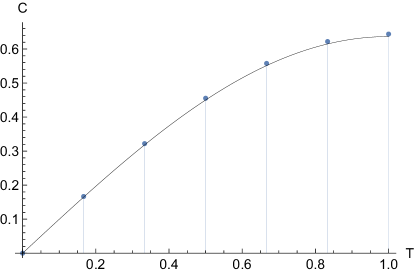
Figure 2: The points give the extremal pairs of value $(\hat{\mathcal{T}}_{k},\hat{\mathcal{C}}_{k})$ for the scenario with $n=6$ outcomes. The line value is the steering bound for a continuous input $\theta$ from the main text. Remarkably at $n=6$ the difference is already almost imperceptible.

The Lemma 2 gives the characterization of the LHS set in the plane $(\hat{\mathcal{T}},\hat{\mathcal{C}})$ in terms of its extremal points $(\hat{\mathcal{T}}_{k},\pm\hat{\mathcal{C}}_{k})$ with $k=0,\dots,n$. This is conceptually appealing, but in the next section it will be easier to use an equivalent characterization in terms of an explicit bound.

Lemma 2 (Steering for discrete setting).

For any LHS model the values of $(\hat{\mathcal{T}},\hat{\mathcal{C}})$ in Eq. (61,60) satisfy

$$|\hat{\mathcal{C}}| \leq\mathcal{B}_{n}(\hat{\mathcal{T}})\leq\frac{\sin\left(\frac{\pi}{2}\hat{\mathcal{T}}\right)}{n\sin\left(\frac{\pi}{2n}\right)}\qquad\text{with}$$ (80)

$$\mathcal{B}_{n}(\hat{\mathcal{T}}) =(1-\hat{\mathcal{T}}n+\lfloor\hat{\mathcal{T}}n\rfloor)\hat{\mathcal{C}}_{\lfloor\mathcal{T}n\rfloor}+(\hat{\mathcal{T}}n-\lfloor\hat{\mathcal{T}}n\rfloor)\hat{\mathcal{C}}_{\lfloor\hat{\mathcal{T}}n\rfloor+1}$$ (81)

$$\hat{\mathcal{C}}_{k} =\frac{\sin\left(\pi\frac{k}{2n}\right)}{n\sin\left(\frac{\pi}{2n}\right)},$$ (82)

where $\mathcal{B}_{n}(\hat{\mathcal{T}})$ is an increasing concave function of $\hat{\mathcal{T}}\in[0,1]$. Furthermore, the bound is saturable.

Proof.

This is just a rewriting on the lemma in a different form. The piece-wise linear function $\mathcal{B}_{n}(\hat{\mathcal{T}})$ is constructed by collecting the line segments connecting the nearby pairs of extremal points $(\hat{\mathcal{T}}_{k},\hat{\mathcal{C}}_{k})$ and $(\hat{\mathcal{T}}_{k+1},\hat{\mathcal{C}}_{k+1})$ for $k=0,\dots,n-1$. The concavity of the function $\mathcal{B}_{n}(\hat{\mathcal{T}})$ follows from the fact that the slope of these line segments is decreasing, i.e. from

$$\hat{\mathcal{C}}_{k+1}-\hat{\mathcal{C}}_{k}\geq\hat{\mathcal{C}}_{k+2}-\hat{\mathcal{C}}_{k+1}\quad\Longleftrightarrow\quad\sin\left(\pi\frac{k+1}{2n}\right)-\sin\left(\pi\frac{k}{2n}\right)\geq\sin\left(\pi\frac{k+2}{2n}\right)-\sin\left(\pi\frac{k+1}{2n}\right)$$ (83)

for all $k=0,\dots,n-2$. The last inequality can be rewritten as

$$\int^{\pi\frac{k+1}{2n}}_{\pi\frac{k}{2n}}\cos(x)\differential x\geq\int^{\pi\frac{k+2}{2n}}_{\pi\frac{k+1}{2n}}\cos(x)\differential x$$ (84)

which is easy to see from the fact that $\cos(x)$ is an decreasing funciton for $x\in\left[0,\frac{\pi}{2}\right]$.

Finally the bound

$$\mathcal{B}_{n}(\hat{\mathcal{T}})\leq G_{n}(\hat{\mathcal{T}}):=\frac{\sin\left(\frac{\pi}{2}\hat{\mathcal{T}}\right)}{n\sin\left(\frac{\pi}{2n}\right)}$$ (85)

follows from the fact that $G_{n}(\hat{\mathcal{T}})$ is a concave function of $\hat{\mathcal{T}}$, and $\mathcal{B}_{n}(\hat{\mathcal{T}})$ is a piece-wise linearization of $G_{n}(\hat{\mathcal{T}})$ on the values $(\hat{\mathcal{T}}_{k},\hat{\mathcal{C}}_{k})=(\hat{\mathcal{T}}_{k},G_{n}(\hat{\mathcal{T}}_{k}))$.

∎

Appendix C CHSH as self-test of Alice’s measurements.

C.1 A priori model of Alice’s measurements

Let $\rho_{AB}$ be the global state shared by Alice and Bob. Since the the measurements that Alice performs on this state are binary, it is convenient to define the two corresponding (Hermitian) observables as

$$A_{x}=\rm{A}_{0|x}-{\rm A}_{1|x}.$$ (86)

In general these measurements are not PVMs (projective). Nevertheless, the usual trick is to dilate them by considering the dilated state $\ket{\rho_{\tilde{A}AB}}$ with $\tr_{\tilde{A}}\rho_{\tilde{A}AB}=\rho_{AB}$, on which the measurements are projective, ${\rm A}_{a|x}={\rm A}_{a|x}^{2}$. Then the operators $A_{x}$ we defined must have eigenvalues $\pm 1$.

By virtue of the Jordan’s lemma Jordan (1875); Scarani (2012) there exists a basis of Hilbert space associated to Alice’s quantum system such that

$$A_{x}=\bigoplus_{\alpha}\left(c_{\alpha}H+(-1)^{x}s_{\alpha}M\right)$$ (87)

where $c_{\alpha}=\cos(\alpha)$, $s_{\alpha}=\sin(\alpha)$, $H=\frac{Z+X}{\sqrt{2}}$, $M=\frac{Z-X}{\sqrt{2}}$, and $X$ with $Z$ are the Pauli operators. We are free to chose the basis inside each qubit block such that $\alpha\in[0,\pi/2]$. This guarantees that $c_{\alpha}$ and $s_{\alpha}$ are positive.

Let $\Pi_{\alpha}$ be the projectors on the qubits blocks in the Jordan decomposition, then by applying the local decoherence map, Alice can prepare the state

$$\bar{\rho}_{AB}=\sum_{\alpha}\Pi_{\alpha}\rho_{AB}\Pi_{\alpha}=\bigoplus_{\alpha}\mu_{\alpha}\,\rho^{\alpha}_{AB},$$ (88)

where $\mu_{\alpha}=\tr\Pi_{\alpha}\rho_{AB}\Pi_{\alpha}$ is a probability density and $\rho^{\alpha}_{AB}=\frac{1}{\mu_{\alpha}}\Pi_{\alpha}\rho_{AB}\Pi_{\alpha}$ is a density operator with a qubit on Alice’s side. The state $\bar{\rho}_{AB}$ is a local post-processing of $\rho_{AB}$ (in particular if it is entangled, $\rho_{AB}$ must be), and they become the sate after the measurements of Alice. Furthermore, since the measurements of Bob are black-box we can assume that all states $\rho_{AB}=\outerproduct{\Psi^{\alpha}}{\Psi^{\alpha}}$ are pure, by introducing their purification and giving it to a third party Eve, on which Bob’s measurements act trivially. From now on we thus assume that the bipartite state before entering the lab of Bob is given by

$$\bar{\rho}_{AB}=\bigoplus_{\alpha}\mu_{\alpha}\outerproduct{\Psi_{\alpha}}{\Psi_{\alpha}}$$ (89)

C.2 CHSH test with Alice and Bob_S  as a self-test of Alice’s device

Consider the CHSH test performed with the measurements $\{A_{a|x}\}_{x}$ and $\{B_{b|y_{S}}^{S}\}_{y_{S}}$ by Alice and Bob_S, respectively. The CHSH score observed in the test

$$\mathcal{S}=\sum_{a,b_{S},x,y_{S}}(-1)^{a+b_{S}+xy_{S}}\,p(a,b_{S}|x,y_{S},S)$$ (90)

can be written in the form $\mathcal{S}=\tr\bar{\rho}_{AB}\Big{(}(A_{0}+A_{1})B^{S}_{0}+(A_{0}-A_{1})B^{S}_{1}\Big{)}$ where we defined the observables $B^{S}_{y_{S}}={\rm B}^{S}_{0|y_{S}}-{\rm B}^{S}_{1|y_{S}}$. With the help of the Jordan form in Eq. (87,89) we obtain $A_{0}+A_{1}=2\bigoplus_{\alpha}c_{\alpha}H$ with $A_{0}-A_{1}=2\bigoplus_{\alpha}s_{\alpha}M,$ and can rewrite the expected CHSH score as

$$\mathcal{S} =\sum_{\alpha}\mu_{\alpha}\,\mathcal{S}_{\alpha}\qquad\text{with}\qquad\mathcal{S}_{\alpha}=2\bra{\Psi_{\alpha}}c_{\alpha}H\otimes B_{0}^{S}+s_{\alpha}M\otimes B_{1}^{S}\ket{\Psi_{\alpha}}\leq 2(c_{\alpha}+s_{\alpha}),$$ (91)

where we used $\|H\otimes B_{0}^{S}\|,\|M\otimes B_{1}^{S}\|\leq 1$.

We summarize the conclusions of the last two sections in the following well-known lemma.

Lemma 3.

In the CHSH test, Alice’s binary measurements and the state can be decomposed as

$$A_{x} =\bigoplus_{\alpha}A_{x}^{\alpha}\quad\text{with}\quad A_{x}^{\alpha}:=c_{\alpha}H+(-1)^{x}s_{\alpha}M$$ (92)

$$\bar{\rho}_{AB} =\bigoplus_{\alpha}\mu_{\alpha}\outerproduct{\Psi_{\alpha}}{\Psi_{\alpha}},$$ (93)

with $\alpha\in\left[0,\frac{\pi}{2}\right]$. Observing a CHSH score of $S$ guarantees that

$$\mathcal{S}\leq 2\sum_{\alpha}\mu_{\alpha}(c_{\alpha}+s_{\alpha}).$$ (94)

Appendix D Routed Bell tests from steering inequalities

In this appendix we prove out main result. In the next section we prove our man result–the routed Bell test in the Eq. (6). Then we present a generalization to the scenario with discrete inputs. But first, we start with a general discussion on SRQ correlations, where the CHSH score in measured in the SP. One notes that this discussion can be easily generalized to any scenario where Alice is restricted to two binary measuremnts.

Recall that SRQ correlation are defined as

$$p(a,b_{r}|x,y_{r},r)\stackrel{{\scriptstyle\rm SRQ}}{{=}}\begin{cases}\tr(\text{A}_{a|x}\otimes\text{B}_{b_{S}|y_{S}}^{S}\,\rho_{AB})&r=S\\ \tr\big(\text{A}_{a|x}\otimes(\sum_{\lambda}p(b_{L}|y_{L},\lambda)\,{\rm E}_{\lambda})\rho_{AB}\big{missing})&r=L\end{cases}.$$ (95)

On top of this Jordan’s lemma implies some structure for Alice’s measurement. Hence, when it is applicable the SRQ correlation can be put in the form

$$p(a,b_{r}|x,y_{r},r)\stackrel{{\scriptstyle\rm SRQ}}{{=}}\begin{cases}\sum_{\alpha}\mu_{\alpha}\tr(\text{A}_{a|x}^{\alpha}\otimes\text{B}_{b_{S}|y_{S}}^{S}\,\rho_{AB}^{\alpha})&r=S\\ \sum_{\alpha}\mu_{\alpha}\tr\big(\text{A}_{a|x}^{\alpha}\otimes(\sum_{\lambda}p(b_{L}|y_{L},\lambda)\,{\rm E}_{\lambda})\rho_{AB}^{\alpha}\big{missing})&r=L\end{cases},$$ (96)

where $\mu_{\alpha}$ is a probability distribution and each $\text{A}_{a|x}^{\alpha}=\frac{1}{2}(\mathds{1}+(-1)^{a}(c_{\alpha}H+(-1)^{x}s_{\alpha}M)$ is a “trusted” qubit measurement. Now we can relax this characterization of SQR correlations by only keeping the information of the CHSH score $\mathcal{S}$ in the SP. With the help lemma 3 this score can be used to constraint the distribution of the distribution of the anle $\alpha$. We thus obtain the following (relaxed) characterization of SRQ correlations

$$p(a,b_{r}|x,y_{r},r)\,\text{is SRQ }\implies\begin{cases}2\sum_{\alpha}\mu_{\alpha}(c_{\alpha}+s_{\alpha})\geq\mathcal{S}\\ p(a,b_{L}|x,y_{L},L)=\sum_{\alpha}\mu_{\alpha}\tr\big(\text{A}_{a|x}^{\alpha}\otimes(\sum_{\lambda}p(b_{L}|y_{L},\lambda)\,{\rm E}_{\lambda})\rho_{AB}^{\alpha}\big{missing})\end{cases}$$ (97)

In turn, to shorten the notation, let us write $p(a,b_{L}|x,y_{L},L)=\sum_{\alpha}\,\mu_{\alpha}p^{\alpha}(a,b_{L}|x,y_{L},L)$, with each distribution $p^{\alpha}$ stems comes from a specific qubit block of Alice

$$p^{\alpha}(a,b_{L}|x,y_{L},L):=\tr\big(\text{A}_{a|x}^{\alpha}\otimes(\sum_{\lambda}p(b_{L}|y_{L},\lambda)\,{\rm E}_{\lambda})\rho_{AB}^{\alpha}\big{missing})=\tr_{A}\big{(}\text{A}_{a|x}^{\alpha}\sum_{\lambda}p(b_{L}|y_{L},\lambda)\rho_{\lambda}^{\alpha}\big{)},$$ (98)

with $\rho_{\lambda}^{\alpha}=\tr_{B}^{\prime}(\mathds{1}\otimes{\rm E}_{\lambda}\,\rho_{AB}^{\alpha})$. Here, the last equality guarantees that each $p^{\alpha}$ admits a LHS model. Let us formalize this observation by introducing the following definition

$${\bf Definition}:\qquad p(a,b|x,y)\text{ is unsteerable for }\text{A}_{a|x}\,\Longleftrightarrow\,p(a,b|x,y)=\tr(\text{A}_{a|x}\sum_{\lambda}p(b|y,\lambda)\rho_{\lambda}),$$ (99)

which is equivalent to unsteerablility of Alice’s assemblage $\rho_{b|y}=\sum_{\lambda}p(b|y,\lambda)\rho_{\lambda}$ if her measurements $\text{A}_{a|x}$ are tomographically complete. Finally, using Eq. (97) we obtain the followings characterization of all SRQ correlation.

Lemma 4.

In the routed scenario of Fig. 1 any SRQ correlation $p(a,b_{r}|x,y_{r},r)$ in Eq. (2) admits the following decomposition

$$p(a,b_{L}|x,y_{L},L)=\sum_{\alpha}\mu_{\alpha}\,p^{\alpha}(a,b_{L}|x,y_{L},L)$$ (100)

$$p^{\alpha}(a,b_{L}|x,y_{L},L)\text{ is unsteerable for }{\rm A}_{a|x}^{\alpha}=\frac{1}{2}(\mathds{1}+(-1)^{a}(c_{\alpha}H+(-1)^{x}s_{\alpha}M)\quad\forall\alpha$$ (101)

$$2\sum_{\alpha}\mu_{\alpha}(c_{\alpha}+s_{\alpha})\geq\mathcal{S}$$ (102)

where $\alpha\in\left[0,\frac{\pi}{2}\right]$, $\mu_{\alpha}$ is a probability distributions and $\mathcal{S}=\sum_{a,b_{S},x,y_{S}}(-1)^{a+b_{S}+xy_{S}}\,p(a,b_{S}|x,y_{S},S)$ in the CHSH score in the SP.

Note that here $\alpha$ may take continuous values, in which case the sums are to be replaced with integrals. This lemma allows one to promote steering inequalities to routed Bell tests, as we now illustrate.

D.1 Proof of the bound in Result 1

To prove the result we are going to show that lemma 4, implies that any SRQ correlation abides to the inequality

$$\mathcal{C}\leq\sin(\pi\frac{\mathcal{T}}{2})\begin{cases}\frac{\mathcal{S}+\sqrt{8-\mathcal{S}^{2}}}{\pi\sqrt{2}}&{\mathcal{S}}>2\\ \frac{2\sqrt{2}}{\pi}&{\mathcal{S}}\leq 2\end{cases}$$ (103)

for the SP CHSH score $\mathcal{S}$ and the LP quantities

$$\mathcal{C} =\int\frac{\differential\theta}{2\pi}\sum_{a,b_{L}=0,1}(-1)^{a+b}\big{(}c_{\theta}p(a,b_{L}|0,\theta,L)+s_{\theta}p(a,b_{L}|1,\theta,L)\big{)}$$ (104)

$$\mathcal{T} =\int\frac{\differential\theta}{2\pi}\sum_{b=0,1}p(b_{L}|\theta)\,.$$ (105)

To do so, for each $p^{\alpha}(a,b_{L}|x,\theta,L)$ let us define the following quantities

$$\hat{\rm c}^{\alpha}(\theta) =\sum_{a,b_{L}=0,1}(-1)^{a+b_{L}}\big{(}c_{\theta}p^{\alpha}(a,b_{L}|0,\theta,L)+s_{\theta}\,p^{\alpha}(a,b_{L}|1,\theta,L)\big{)}$$ (106)

$$\hat{\rm t}^{\alpha}(\theta) =\sum_{b_{L}=0,1}p^{\alpha}(b_{L}|\theta)=\sum_{a,b_{L}=0,1}p^{\alpha}(a,b_{L}|x,\theta,L)$$ (107)

as well as their averages with respect to $\theta$

$$\hat{\mathcal{T}}^{\alpha}=\int\frac{\differential\theta}{2\pi}\hat{\rm t}^{\alpha}(\theta)\qquad\hat{\mathcal{C}}^{\alpha}=\int\frac{\differential\theta}{2\pi}\hat{\rm c}^{\alpha}(\theta).$$ (108)

By virtue of Eq. (100) these quantities can be related to the observed values by averaging aver $\alpha$

$$\hat{\mathcal{T}}=\sum_{\alpha}\mu_{\alpha}\,\hat{\mathcal{T}}^{\alpha}\qquad\hat{\mathcal{C}}=\sum_{\alpha}\mu_{\alpha}\,\hat{\mathcal{C}}^{\alpha}.$$ (109)

Now, we also know (Eq. 101) that the correlations $p^{\alpha}(a,b_{L}|x,\theta,L)$ are unsteerable with the measurements ${\rm A}^{\alpha}_{a|x}$ performed by Alice. In other words they admits a LHS model leading to the unsteerable assemblage $\rho_{b_{L}|\theta}^{\alpha}=\sum_{\lambda}p(b_{L}|\theta,\lambda)\rho_{\lambda}^{\alpha}$ on Alice’s side, leading to

$$p^{\alpha}(a,b_{L}|x,\theta,L)=\frac{1}{2}\tr\big((\mathds{1}+(-1)^{a}A_{x}^{\alpha})\rho_{b_{L}|\theta}\big{missing})\qquad\text{with}\qquad A_{x}^{\alpha}=c_{\alpha}\frac{Z+X}{\sqrt{2}}+(-1)^{x}s_{\alpha}\frac{Z-X}{\sqrt{2}}.$$ (110)

Straightforward algebra allows us to express the quantities $\hat{\rm t}^{\alpha}(\theta)$ and $\hat{\rm c}^{\alpha}(\theta)$ with the help of these states $\rho_{b_{L}|\theta}^{\alpha}$ and the qubit observable $A_{x}^{\alpha}$ as

$$\hat{\rm t}^{\alpha}(\theta) =\tr(\rho^{\alpha}_{0|\theta}+\rho^{\alpha}_{1|\theta})$$ (111)

$$\hat{\rm c}^{\alpha}(\theta) =\tr\big((\rho^{\alpha}_{0|\theta}-\rho^{\alpha}_{1|\theta})\left(C_{\alpha}(c_{\theta}Z+s_{\theta}X)+S_{\alpha}(s_{\theta}Z+c_{\theta}X)\right)\big{missing})$$

where we introduced the trigonometric functions $C_{\alpha}:=\frac{c_{\alpha}+s_{\alpha}}{\sqrt{2}}\in[0,1]$ and $S_{\alpha}:=\frac{c_{\alpha}-s_{\alpha}}{\sqrt{2}}\in[-1,1]$. Then, when averaging over $\theta$ we find

$$\hat{\mathcal{T}}^{\alpha} =\int\frac{\differential\theta}{2\pi}\tr(\rho^{\alpha}_{0|\theta}+\rho^{\alpha}_{1|\theta})$$ (112)

$$\hat{\mathcal{C}}^{\alpha} =C_{\alpha}\hat{\mathcal{C}}_{1}^{\alpha}+S_{\alpha}\hat{\mathcal{C}}_{2}^{\alpha}$$ (113)

$$\hat{\mathcal{C}}_{1}^{\alpha} =\int\frac{\differential\theta}{2\pi}\tr\big((\rho^{\alpha}_{0|\theta}-\rho^{\alpha}_{1|\theta})(c_{\theta}Z+s_{\theta}X)\big{missing})$$ (114)

$$\hat{\mathcal{C}}_{2}^{\alpha} =\int\frac{\differential\theta}{2\pi}\tr\big((\rho^{\alpha}_{0|\theta}-\rho^{\alpha}_{1|\theta})(s_{\theta}Z+c_{\theta}X)\big{missing}).$$ (115)

Since the states $\rho_{b_{L}|\theta}^{\alpha}$ are prepared with an LHS these quantities satisfy the steering inequality given by the Lemma 1, implying $|\hat{\mathcal{C}}_{1}^{\alpha}|,\,|\hat{\mathcal{C}}_{2}^{\alpha}|\leq\frac{2}{\pi}\sin(\pi\frac{\hat{\rm T}^{\alpha}}{2})$ (to see this explicitly for $\hat{\mathcal{C}}_{2}^{\alpha}$ one can introduce a simple coordinate change $\theta\to\frac{\pi}{2}-\theta$ in the integrals and the labeling of Bob’s setting). Combining the two inequalities we find that following bound

$$\hat{\mathcal{C}}^{\alpha}\leq(C_{\alpha}+|S_{\alpha}|)\frac{2}{\pi}\sin(\pi\frac{\hat{\mathcal{T}}^{\alpha}}{2})=\left(C_{\alpha}+\sqrt{1-C_{\alpha}^{2}}\right)\frac{2}{\pi}\sin(\pi\frac{\hat{\mathcal{T}}^{\alpha}}{2})$$ (116)

must hold for any $p^{\alpha}(a,b_{L}|x,\theta,L)$ unsteerable for ${\rm A}_{a|x}^{\alpha}$. Plugging this bound togetehr with Eq. (109) into Lemma 4, implies that for any SRQ correlation $p^{\alpha}(a,b_{r}|x,y_{r},r)$, the quantities $\mathcal{S},\mathcal{C}$ and $\mathcal{T}$ must satisfy the following optimization must be feasible

$$\min_{\mu_{\alpha},C_{\alpha},\hat{\mathcal{C}}^{\alpha},\hat{\mathcal{T}}^{\alpha}}\qquad 1$$ (117)

such that $$\hat{\mathcal{C}}^{\alpha}\leq\left(C_{\alpha}+\sqrt{1-C_{\alpha}^{2}}\right)\frac{2}{\pi}\sin(\pi\frac{\hat{\mathcal{T}}^{\alpha}}{2})$$ (118)

$$\mathcal{C}=\sum_{\alpha}\mu_{\alpha}\hat{\mathcal{C}}^{\alpha}$$ (119)

$$\mathcal{T}=\sum_{\alpha}\mu_{\alpha}\hat{\mathcal{T}}^{\alpha}$$ (120)

$$\sum_{\alpha}\mu_{\alpha}C_{\alpha}\geq\frac{\mathcal{S}}{2\sqrt{2}}$$ (121)

To solve this, one notes that the two-variables function

$$F(C_{\alpha},\hat{\mathcal{T}}^{\alpha}):=\left(C_{\alpha}+\sqrt{1-C_{\alpha}^{2}}\right)\frac{2}{\pi}\sin(\pi\frac{\hat{\mathcal{T}}^{\alpha}}{2})$$ (122)

in the first constraint is concave, since it is a product of two single-variable concave functions. Using this property we must have

$$\hat{\mathcal{C}}=\sum_{\alpha}\mu_{\alpha}\,\hat{\mathcal{C}}^{\alpha}\leq\sum_{\alpha}\mu_{\alpha}F(C_{\alpha},\hat{\mathcal{T}}^{\alpha})\leq F\left(\sum_{\alpha}\mu_{\alpha}C_{\alpha},\mathcal{T}s\right).$$ (123)

This allows us to relax the feasibility program to

$$\min_{\mu_{\alpha},C_{\alpha}}\qquad 1$$ (124)

such that $$\mathcal{C}\leq F\left(\sum_{\alpha}\mu_{\alpha}C_{\alpha},\mathcal{T}\right)$$ (125)

$$\sum_{\alpha}\mu_{\alpha}C_{\alpha}\geq\frac{\mathcal{S}}{2\sqrt{2}}.$$ (126)

Here $F(C,\mathcal{T})$ is maximized at $C=\frac{1}{\sqrt{2}}$, hence for $\frac{\mathcal{S}}{2\sqrt{2}}\leq\frac{1}{\sqrt{2}}$ is below this value, the program is feasible iff $\mathcal{C}\leq F\left(\frac{1}{\sqrt{2}},\mathcal{T}\right).$ In turn, when $\frac{\mathcal{S}}{2\sqrt{2}}>\frac{1}{\sqrt{2}}$, setting $C=\sum_{\alpha}\mu_{\alpha}C_{\alpha}=\frac{1}{\sqrt{2}}$ is incompatible with the CHSH constraint. In this case since $F(C,\mathcal{T})$ is decreasing with $C\in\left[\frac{1}{\sqrt{2}},1\right]$, the program is feasible iff $\mathcal{C}\leq F\left(\frac{\rm S}{2\sqrt{2}},{\rm T}\right)$. Combining the two cases, we conclude that the program is feasible iff

$$\mathcal{C}\leq\begin{cases}F\left(\frac{\mathcal{S}}{2\sqrt{2}},{\mathcal{T}}\right)&{\mathcal{S}}>2\\ F\left(\frac{\rm 1}{\sqrt{2}},{\mathcal{T}}\right)&{\mathcal{S}}\leq 2.\end{cases}$$ (127)

This is precisely the expression in Eq. (103), which must thus hold for all SRQ correlations. This proves the the first part of the theorem. We now also show that the bound can be saturated by an SRQ model.

D.2 Proof of the tigtness of the bound in Result 1

We now construct an SRQ model saturating the bound. Take any $\alpha\in[0,\frac{\pi}{4}]$ (with $S_{\alpha}=\frac{c_{\alpha}-s_{\alpha}}{\sqrt{2}}\geq 0$). Let the source prepare the maximally entangled state $\ket{\Phi^{+}}=\frac{1}{\sqrt{2}}(\ket{00}+\ket{11})$ and let Alice’s measurements be precisely the ones given by the Jordan’s lemma

$$\hat{A}_{x}^{\alpha}=\left(c_{\alpha}H+(-1)^{x}s_{\alpha}M\right).$$ (128)

With this state and these measurements of Alice chosing the optimal measurements of Bob_S  give the CHSH score (see e.g. the derivation of Lemma 3)

$$\mathcal{S}=2\sqrt{2}\left(\frac{c_{\alpha}+s_{\alpha}}{\sqrt{2}}\right)=2\sqrt{2}\,C_{\alpha}.$$ (129)

We let Bob_S  these measurements.

Now after the router in the LP we perform a two-outcomes measurement $\{{\rm E}_{\lambda}\}$ in the eigenbasis of $H=\frac{Z+X}{\sqrt{2}}$. By doing so, and observing an output $\lambda=\pm 1$ (with equal probability) collapses Alice’s reduced state to

$$\varrho_{\pm}=\frac{1}{2}\left(\mathds{1}\pm H\right).$$ (130)

A copy of the value $\lambda$ is sent to the device of Bob_L  (manisfestly there is no entanglement shared between Alice and Bob_L) which instructs his measurement apparatus to implement some deterministic response function $p(b_{L}|\lambda,\theta)\in\{0,1\}$, which we assume to satisfy $p(0|\pm,\theta)=p(1|\mp,\theta)$. This is an LHS model that after Bob_L’s measurement leaves Alice’s qubit in a state

$$\rho_{b_{L}|\theta}=\frac{1}{2}\left(p(b_{L}|+,\theta)\varrho_{+}+p(b_{L}|-,\theta)\varrho_{-}\right).$$ (131)

In particular, let us now compute the following quantities

$${\rm t}(\theta) =\sum_{b_{L}=0,1}p(b_{L}|\theta)=\tr(\rho_{0|\theta}+\rho_{1|\theta})=\frac{p(0|+,\theta)+p(1|+,\theta)+p(0|-,\theta)+p(1|-,\theta)}{2}$$ (132)

$$\rho_{0|\theta}-\rho_{1|\theta} =\frac{p(0|+,\theta)-p(1|+,\theta)}{2}\varrho_{+}-\frac{p(1|-,\theta)-p(0|-,\theta)}{2}\varrho_{-}$$ (133)

$$=\frac{p(0|+,\theta)-p(1|+,\theta)}{2}(\varrho_{+}-\varrho_{-})$$ (134)

$$=(-1)^{s(\theta)}\frac{{\rm t}(\theta)}{2}H$$ (135)

where we used $p(0|\pm,\theta)=p(1|\mp,\theta)$, and the fact that we are free to chose the sign $s(\theta)\in\{0,1\}$ in the last equality by setting either $p(0|+,\theta)$ or $p(1|+,\theta)$ equal to one (if $p(\varnothing|+,\theta)=1$ then ${\rm t}(\theta)=0$ and the sign does not matter). Next, noting that

$$\tr H\left(C_{\alpha}(c_{\theta}Z+s_{\theta}X)+S_{\alpha}(s_{\theta}Z+c_{\theta}X)\right)=\sqrt{2}(C_{\alpha}+S_{\alpha})(c_{\theta}+s_{\theta})=2(C_{\alpha}+S_{\alpha})\sin(\frac{\pi}{4}+\theta)$$ (136)

we compute the quantities $\mathcal{T}$ and $\mathcal{C}$ achieved by our SRQ model

$$\mathcal{T} =\int\frac{\differential\theta}{2\pi}{\rm t}(\theta)$$ (137)

$$\mathcal{C} =\int\frac{\differential\theta}{2\pi}\tr(\rho_{0|\theta}-\rho_{1|\theta})\left(C_{\alpha}(c_{\theta}Z+s_{\theta}X)+S_{\alpha}(s_{\theta}Z+c_{\theta}X)\right)$$ (138)

$$=(C_{\alpha}+S_{\alpha})\int\frac{\differential\theta}{2\pi}(-1)^{s(\theta)}\sin(\frac{\pi}{4}+\theta){\rm t}(\theta)$$ (139)

$$=(C_{\alpha}+S_{\alpha})\int\frac{\differential\theta}{2\pi}\left|\sin(\frac{\pi}{4}+\theta)\right|{\rm t}(\theta)$$ (140)

where we chose $s(\theta)$ to compensate the sign of the sinus.

Next, let us find ${\rm t}(\theta)$ maximizing $\mathcal{C}$ for a given $\mathcal{T}$. It is straightforward to see that this is the one which gives a conclusive outcome $(b_{L}\neq\varnothing)$ when $\left|\sin(\frac{\pi}{4}+\theta)\right|$ takes its largest values, i.e. by choosing

$${\rm t}(\theta)=\begin{cases}1&(\frac{\pi}{4}+\theta)\in[\frac{\pi}{2}-\Omega,\frac{\pi}{2}+\Omega]\cup[\frac{3\pi}{2}-\Omega,\frac{3\pi}{2}+\Omega]\\ 0&\text{otherwise}\end{cases}$$ (141)

for some parameter $\Omega\in[0,\pi/2]$. Straightforward integration shows that this SRQ model achaives the values

$$\mathcal{T} =\frac{\Omega}{\pi/2}$$ (142)

$$\mathcal{C} =(C_{\alpha}+S_{\alpha})\frac{\sin(\Omega)}{\pi/2}=(C_{\alpha}+S_{\alpha})\frac{\sin(\mathcal{T}\,\pi/2)}{\pi/2}.$$ (143)

Recalling that by varying the angle $\alpha$ we can also have $C_{\alpha}=\frac{\mathcal{S}}{2\sqrt{2}}$ and hence $S_{\alpha}=\frac{\sqrt{8-\mathcal{S}^{2}}}{2\sqrt{2}}$. Plugging this into Eq. (143) we conclude that our SQR model can saturate

$$\mathcal{C}=\frac{\mathcal{S}+\sqrt{8-\mathcal{S}^{2}}}{\pi\sqrt{2}}\sin(\mathcal{T}\frac{\pi}{2}),$$ (144)

for any CHSH score $\mathcal{S}\in[2,2\sqrt{2}]$ and $\mathcal{T}\in[0,1]$. This concludes the proof.

The case $\mathcal{S}\leq 2$ is remarkable in the sense that here the CHSH score plays no role. Hence,

$$\mathcal{C}\leq\frac{2\sqrt{2}}{\pi}\sin(\mathcal{T}\frac{\pi}{2})$$ (145)

is a regular Bell inequality. Since in our setup Alice only has two binary measurements, it is known that $p(a,b_{L}|x,\theta,L)$ is nonlocal if and only if it violates the CHSH test (for some pair of Bob_L’s settings $\theta_{0}$ and $\theta_{1}$).

D.3 Routed Bell inequalities for Bob_L  with discrete inputs.

Let us now slightly modify the setting of the Result 1 such that Bob_L  has a finite number $n$ of measuremtn setttings labeled by $\theta_{i}$ with $i=0,\dots n-1$. Then for the LP correlations we define the following quantities

$$\mathcal{C} =\frac{1}{n}\sum_{i=0}^{n-1}\sum_{a,b_{L}=0,1}(-1)^{a+b_{L}}\left(c_{\theta_{i}}p(a,b_{L}|0,\theta_{i},L)+s_{\theta_{i}}p(a,b_{L}|1,\theta_{i},L)\right)$$ (146)

$$\mathcal{T} =\frac{1}{n}\sum_{i=0}^{n-1}\sum_{b_{L}=0,1}p(b_{L}|\theta_{i},L),$$ (147)

where we essentially replaced an integral over $\theta$ with a discrete sum over $\theta_{i}$. With the help of the discrete steering inequality (80) we now show the following routed Bell inequality.

Result 2.

In the routed Bell scenario of Fig. 1 the SP CHSH score $\mathcal{S}$ in Eq. (3), and the LP quuantities $\mathcal{C}$ and $\mathcal{T}$ in Eqs. (146, 147) satisfy

$$\mathcal{C}\quad\leq\quad\mathcal{B}_{n}(\mathcal{T})\begin{cases}\frac{\mathcal{S}+\sqrt{8-\mathcal{S}^{2}}}{2\sqrt{2}}&\mathcal{S}>2\\ \sqrt{2}&\mathcal{S}\leq 2\end{cases}\quad\leq\quad\frac{\sin\left(\frac{\pi}{2}\hat{\mathcal{T}}\right)}{n\sin\left(\frac{\pi}{2n}\right)}\begin{cases}\frac{\mathcal{S}+\sqrt{8-\mathcal{S}^{2}}}{2\sqrt{2}}&\mathcal{S}>2\\ \sqrt{2}&\mathcal{S}\leq 2\end{cases}$$ (148)

for any SRQ correlations. Where the function $\mathcal{B}_{n}$ is defined in Eq. (81), and $n$ is the number of measurement settings of Bob_L.

Proof.

This result can be proven by following the steps of the Sec.  almost identically. So here we will only highlight the differences.

Naturally, the starting point is the Lemma. 4 and the decomposition $p(a,b_{L}|x,y_{L},L)=\sum_{\alpha}\mu_{\alpha}\,p^{\alpha}(a,b_{L}|x,y_{L},L)$. However we now work with different quantities

$$\hat{\mathcal{T}}^{\alpha} =\frac{1}{n}\sum_{i=0}^{n-1}\sum_{a,b_{L}=0,1}p(a,b_{L}|x,\theta_{i},L)=\frac{1}{n}\sum_{i=0}^{n-1}\hat{\rm t}^{\alpha}(\theta_{i})=\frac{1}{n}\sum_{i=0}^{n-1}\tr(\rho^{\alpha}_{0|\theta_{i}}+\rho^{\alpha}_{1|\theta_{i}})$$ (149)

$$\hat{\mathcal{C}}^{\alpha} =\frac{1}{n}\sum_{i=0}^{n-1}\sum_{a,b_{L}=0,1}(-1)^{a+b_{L}}\,(c_{\theta_{i}}p^{\alpha}(a,b_{L}|0,\theta_{i},L)+s_{\theta_{i}}p^{\alpha}(a,b_{L}|1,\theta_{i},L)=\frac{1}{n}\sum_{i=0}^{n-1}\hat{\rm c}^{\alpha}(\theta_{i})=C_{\alpha}\hat{\mathcal{C}}_{1}^{\alpha}+S_{\alpha}\hat{\mathcal{C}}_{2}^{\alpha}$$ (150)

$$\hat{\mathcal{C}}_{1}^{\alpha} =\frac{1}{n}\sum_{i=0}^{n-1}\tr\{(\rho^{\alpha}_{0|\theta_{i}}-\rho^{\alpha}_{1|\theta_{i}})(c_{\theta_{i}}Z+s_{\theta_{i}}X)\big{\}}$$ (151)

$$\hat{\mathcal{C}}_{2}^{\alpha} =\frac{1}{n}\sum_{i=0}^{n-1}\tr\{(\rho^{\alpha}_{0|\theta_{i}}-\rho^{\alpha}_{1|\theta_{i}})(s_{\theta_{i}}Z+c_{\theta_{i}}X)\big{\}}.$$ (152)

Since each $p^{\alpha}(a,b_{L}|x,y_{L},L)$ admits a LHS model, the quantities $(\hat{\mathcal{T}}^{\alpha},\hat{\mathcal{C}}_{1}^{\alpha})$ and $(\hat{\mathcal{T}}^{\alpha},\hat{\mathcal{C}}_{2}^{\alpha})$ must satisfy the steering inequality (80), implying

$$\hat{\mathcal{C}}^{\alpha}\leq(C_{\alpha}+S_{\alpha})\mathcal{B}_{n}(\hat{\mathcal{T}}^{\alpha})=(C_{\alpha}+\sqrt{1-C_{\alpha}^{2}})\mathcal{B}_{n}(\mathcal{T}^{\alpha}).$$ (153)

Therefore for any SRQ model, the following program must be feasible

$$\min_{\mu_{\alpha},C_{\alpha},\hat{\mathcal{C}}^{\alpha},\hat{\mathcal{T}}^{\alpha}}\qquad 1$$ (154)

such that $$\hat{\mathcal{C}}^{\alpha}\leq\left(C_{\alpha}+\sqrt{1-C_{\alpha}^{2}}\right)\mathcal{B}_{n}(\hat{\mathcal{T}}^{\alpha})$$ (155)

$$\mathcal{C}=\sum_{\alpha}\mu_{\alpha}\hat{\mathcal{C}}^{\alpha}$$ (156)

$$\mathcal{T}=\sum_{\alpha}\mu_{\alpha}\hat{\mathcal{T}}^{\alpha}$$ (157)

$$\sum_{\alpha}\mu_{\alpha}C_{\alpha}\geq\frac{\mathcal{S}}{2\sqrt{2}}.$$ (158)

As before the function on the rhs of the first constraint is concave in both variables $C_{\alpha}$ and $\hat{\mathcal{T}}^{\alpha}$, so the program can be relaxed to

$$\min_{\mu_{\alpha},C_{\alpha}}\qquad 1$$ (159)

such that $$\mathcal{C}\leq\left(C_{\alpha}+\sqrt{1-C_{\alpha}^{2}}\right)\mathcal{B}_{n}(\mathcal{T})$$ (160)

$$\sum_{\alpha}\mu_{\alpha}C_{\alpha}\geq\frac{\mathcal{S}}{2\sqrt{2}}.$$ (161)

In turn, just like for the program in Eq. (124) one can show that it it feasible iff

$$\mathcal{C}\leq\mathcal{B}_{n}(\mathcal{T})\begin{cases}\frac{\mathcal{S}+\sqrt{8-\mathcal{S}^{2}}}{2\sqrt{2}}&\mathcal{S}>2\\ \sqrt{2}&\mathcal{S}\leq 2.\end{cases}$$ (162)

The second inequality in (148) follows from the upper bound on $\mathcal{B}_{n}(\mathcal{T})$ provided by the Eq. (80). This concludes the proof and this manuscript. ∎