Bondi-like Accretion Flow Dynamics: The Role of Gravitational Potential

Abstract

The formation of massive black holes and their coevolution with host galaxies are pivotal areas of modern astrophysics. Spherical accretion onto a central point mass serves as a foundational framework in cosmological simulations, semianalytical models, and observational studies. This work extends the classical spherical accretion model by incorporating the gravitational potential of host galaxies, including contributions from stellar components and dark matter halos. Numerical solutions spanning parsec-scale to event-horizon-scale regimes reveal that the flow structure is highly sensitive to the mass and size of the dark matter halo. Adding low angular momentum to the accreting gas demonstrates that such flows resemble spherical Bondi accretion, with mass accretion rates converging towards the Bondi rate. We find that the low angular momentum flow resembles the spherical Bondi flow and its mass accretion rate approaches the Bondi accretion rate. Due to the presence of dark matter, the mass accretion rate is increased by a factor of more than $\sim\%100$ in comparison to analogous hydrodynamic solutions. These findings underscore the critical role of stellar and dark matter gravitational potentials in shaping the dynamics and accretion rates of quasi-spherical flows, providing new insights into astrophysical accretion processes.

1 Introduction

Almost every galaxy hosts a super massive black hole (SMBH). Black hole accretion systems, such as X-ray binariess or active galactic nucleis, have the capacity to release significant amounts of energy into the interstellar medium. The mass of a black hole is closely correlated with various properties of its host galaxy, indicating a co-evolution between the central black hole (BH) and its host galaxy Tremaine et al. (2002); Kormendy & Ho (2013). However, it remains largely unknown how black holes are connected to their larger-scale environments and host dark matter halos. It has been suggested that several mechanisms drive gas into the galaxy’s center, eventually triggering AGN activity, which depends on either the galaxy’s cosmic environments or the dark matter halos that host them Hopkins et al. (2008). Understanding these mechanisms could also provide insights into galaxy cluster formation, particularly for low-luminosity AGNs, where accretion dynamics deviate from standard models.

In recent decades, numerous analytical models have been developed to elucidate the fundamental physical processes occurring within the accretion flow. The simplest model for accretion is spherical accretion, which assumes a spherically symmetric inflow Bondi (1952) accretion model, while being a useful mathematical construct, represents an idealized scenario. In reality, angular momentum, even if minimal, plays a key role in determining accretion dynamics. Deviations from idealized spherical flows, especially in the presence of small angular momentum or environmental complexities remains an important avenue for research.

The classical Bondi problem has been instrumental in analyzing accretion onto primordial black holes in the early universe, before the formation of galaxies and stars Ricotti (2007). The central AGN is typically located in the densest region of a cluster’s hot atmosphere. Consequently, the classical Bondi accretion of hot gas is often considered a primary fueling mechanism for black holes. Narayan & Fabian (2011) introduced an accretion flow known as the slowly rotating accretion flow. This model serves as an intermediate case between Bondi accretion and the advection-dominated accretion flow (ADAF), making it particularly relevant to the central regions of elliptical galaxies, where the accretion rate closely mirrors that of Bondi accretion. Extending such frameworks to include time-dependent processes or magnetohydrodynamic (MHD) effects could enhance their relevance to AGN observations.

A spherical or quasi-spherical flow has no angular momentum, so the loss of angular momentum is not essential for accretion. Bondi flows with purely spherical surfaces or flows with angular momentum below the minimum value in circular orbits around black holes are examples of such solutions. Recent investigations of Bondi accretion and quasi-spherical accretion have given considerable attention to the influence of the gravitational potential exerted by the stars within the galaxy Ciotti & Pellegrini (2017, 2018); Samadi et al. (2019); Ranjbar & Abbassi (2023). However, as our solution involves large-scale distances, the potential impact of dark matter cannot be overlooked. This study aims to investigate the significance of dark matter in the dynamics and structure of Bondi and Bondi-like accretion.

The classical Bondi solution is used in the interpretation of observational results, in numerical investigations, or in cosmological simulations involving galaxies and accretion on their central BHs. In many such studies, when the instrumental resolution is limited, or the numerical resolution is inadequate, an estimate of the mass accretion rate is derived using the classical Bondi solution, taking values of temperature and density measured at some finite distance from the BH. This procedure clearly produces an estimate that can depart from the true value, even when assuming that accretion fulfills the hypotheses of the Bondi model (stationarity, spherical symmetry, etc.). Ranjbar & Abbassi (2023) developed the analytical setup of the problem for generic accretion from classical Bondi accretion to the inclusion of the additional effects of galactic potential and slow rotation and outflow; We also numerically investigated the deviation of mass accretion rate from Bondi rate in presence of rotation. Here we reconsider the problem for the Bondi-like case in the presence of a dark matter halo that was not discussed in detail in Ranjbar & Abbassi (2023) and extend the investigation also to the case of the Hernquest potential.

In addition to these considerations, the gravitational potential of the host galaxy, which includes stellar and dark matter components of galaxies, must also be taken into account when studying accretion flows on scales beyond those of black holes. Estimating the influence of the host galaxy’s gravitational potential requires complex calculations, a factor frequently overlooked in previous research.

Many galaxies are known to be enveloped by dark matter, and it is reasonable to expect that black holes and their accretion flows are similarly surrounded by dark matter halos. The distribution of dark matter can vary depending on the mass and type of the galaxy. Among the various profiles used to describe dark matter, the NFW (Navarro-Frenk-White) Navarro et al. (1996), Hernquist Hernquist (1990), Jaffe Jaffe (1983), and King King (1962) profiles are widely recognized. For the present study, we specifically consider the Hernquist profile, which represents a simple and spherical model, offering a basic representation of dark matter in elliptical galaxies. The gravitational response of black holes in the astrophysical environment was tested with this model Cardoso et al. (2022).

Observations indicate that the distribution of both the stellar (baryonic matter) and dark matter components within galaxies is such that their total mass profile is evident over a large radial distance (e.g., Treu & Koopmans (Treu & Koopmans (2002), 2004); Gavazzi et al. (2007)). A physical process at a sub-pc and pc scale can be complex in reality. Based on observations, an SMBH of $\sim 10^{8}-10^{9}M_{\odot}$ is embedded in a stellar bulge of the size of a few $10^{2}pc$, e.g. Philipp et al. (1999). Close to the BH, its gravitational potential drastically influences the movement of stars and the interstellar medium. However, at larger distances, the gravitational impact of the BH on the overall dynamics of stellar and interstellar medium diminishes significantly. In such scenarios, alongside the BH’s potential, the gravitational potential of the galaxy stars becomes consequential on the parsec scale and must be taken into account. At larger scales, such as the galaxy scale, it is essential to incorporate the gravitational potential of host galaxies Yang & Bu (2018), Bu et al. (2016), Sun & Yang (2021). Previous studies have explored Bondi accretion at the galaxy scale, considering the influence of the host galaxy’s gravitational potential ((Barai et al., 2011; Korol et al., 2016; Ciotti & Pellegrini, 2017)). In this paper, our focus will be on investigating the impact of both the dark matter halo and the gravitational potential of the stars on Bondi-like accretion. Apart from the gravitational influence of the galaxy potential, the presence of dark matter can also exert an impact on the structural characteristics of the accretion flow. However, this problem has not received enough attention until now.

In this study, our aim is to systematically study how adding dark matter potential plus bulge stars potential to the equation of motion of Bondi accretion impacts its structure and mass accretion rate. Additionally, we explore the influence of the dark matter potential on a slowly rotating accretion flow. Ultimately, we seek to understand the impact of low angular momentum and dark matter potential on spherical accretions. By employing more realistic gravitational potentials, we aim to explore their effects on the characteristics of different accretion solution types. In our solution, the outer boundary is exactly in the Bondi radius.

The paper is organized as follows. In section 2, we consider the generalized case of Bondi-like accretion in the presence of galaxy potential hosting the central BH 2.2. Section 3 presents the equations for accretion flow with low angular momentum. In Section 4, we present the numerical results obtained from our study. Finally, in Section 5, we discuss the implications and findings of our results. and technical details are given in the appendix.

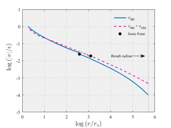
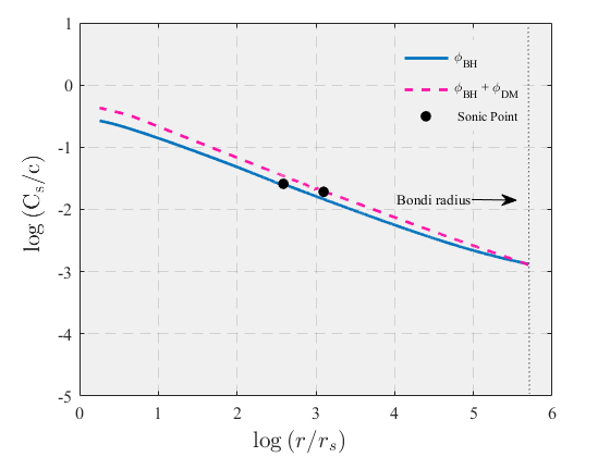
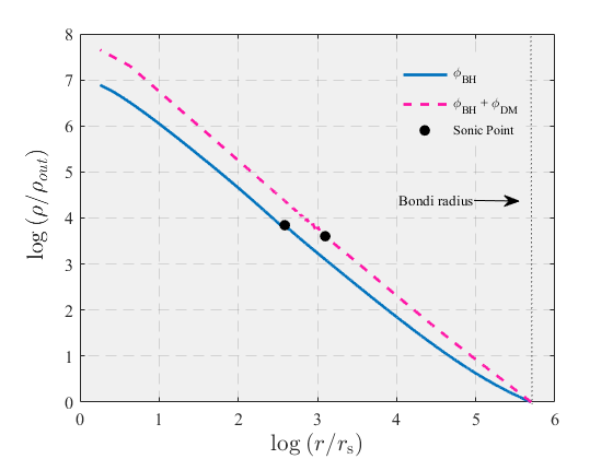
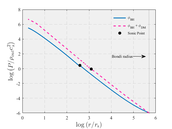
Figure 1: Global solutions for Bondi accretion, $\gamma=5/3$, $M_{halo}=M_{BH}$, $a=100$. Blue line related without dark matter potential,($\phi_{DM}=0,r_{c}=386.74$). Dashed pink line ($\phi_{DM}\neq 0,r_{c}=1253.6$). Galaxy potential is $\phi_{galaxy}\neq 0$. A solid dot indicates the position of the critical point. The vertical dotted lines correspond to the location of the Bondi radius $r_{B}$.

2 Bondi-like Flow

The mechanisms by which SMBHs in galactic nuclei are fed remain uncertain. For spherically symmetric accretion of hot gas Bondi (1952), the accretion begins from a characteristic radius, known as the Bondi radius, defined as:

$$r_{B}=\frac{2GM_{BH}}{c_{s,\infty}^{2}},$$ (1)

where $G$ is the gravitational constant, $M_{BH}$ is the black hole mass, and $c_{s,\infty}$ is the sound speed of the ambient gas. At this radius, the gravitational energy due to the SMBH becomes comparable to the thermal energy of the gas. The Bondi radius represents the scale at which the SMBH’s gravitational influence transitions from negligible to dominant, offering a natural framework for modeling accretion flows.

In this section, we calculate the dynamics of accreting matter in the combined gravitational potential of a host galaxy and a central black hole, assuming a steady-state, spherically symmetric flow (i.e., no angular momentum). We consider the simplest case: spherically symmetric steady accretion under the gravitational field of a black hole plus host galaxy (i.e. stars plus dark matter). The inclusion of both stellar and dark matter gravitational potentials allows for a more comprehensive understanding of accretion dynamics at scales beyond the immediate vicinity of the SMBH, bridging the gap between galactic and sub-galactic scales. Spherical accretion onto a gravitating body was first studied by Bondi (1952) and is often called Bondi accretion, which is now believed to be quite significant. While the classical Bondi model is invaluable for its simplicity and mathematical elegance, it has limitations when applied to realistic astrophysical scenarios. These include neglecting the influence of large-scale gravitational potentials, angular momentum, and potential radiative feedback effects. Extending the Bondi framework to account for such complexities can significantly enhance its applicability to modern observations and simulations. Our analysis incorporates the combined gravitational potential of the black hole, stellar bulge, and dark matter halo. This multi-component approach enables us to study how each component contributes to the accretion dynamics, offering insights into the coupling between small-scale and large-scale astrophysical processes. The solutions derived here serve as a baseline for understanding more intricate accretion scenarios, including rotating and radiatively inefficient flows.

2.1 Basic Equations

We consider a spherically symmetric flow around a black hole embedded in a dark matter halo. The flow is assumed to be steady and one-dimensional in the radial ($r$) direction. The magnetic and radiation fields are neglected, and the flow is further assumed to be inviscid and adiabatic. Under the Newtonian approximation, the continuity equation and the equation of motion of this infalling matter are given by:

$$\frac{1}{4\pi r^{2}}\frac{d}{dr}(\rho vr^{2})=0,$$ (2)

$$v\frac{dv}{dr}=-\frac{d\Phi}{dr}-\frac{1}{\rho}\frac{dp}{dr},$$ (3)

where $\Phi$ is the gravitational potential (for more details, see 2.2), $v$ is the flow velocity (negative for accretion), $\rho$ is the density, and $p$ is the pressure. These equations form the foundation for describing spherical accretion in the combined gravitational field of the black hole and the host galaxy, allowing us to explore the impact of dark matter and stellar potentials on the dynamics.

Integrating these equations yields the continuity equation:

$$-4\pi\rho vr^{2}=\dot{M},$$ (4)

where $\dot{M}$ is the mass accretion rate, which is constant in this case. This result implies a steady inflow of mass, with the accretion rate governed by the density and velocity profiles of the gas. In spherical accretion flow, the entropy of the gas remains constant:

$$S_{in}=\frac{c_{s}^{2}}{\rho^{\gamma-1}}=\text{constant},$$ (5)

where $c_{s}$ is the sound speed $c_{s}=(p/\rho)^{1/2}$, and $\gamma$ is the ratio of specific heat of the gas, set to be $\gamma=5/3$. This assumption ensures that the flow remains adiabatic, a reasonable approximation for many astrophysical accretion scenarios. Consequently, the Bernoulli equation is given by:

$$\frac{1}{2}v^{2}+\Phi+\frac{\gamma S_{in}}{(\gamma-1)r^{2(\gamma-1)}v^{\gamma-1}}\left(\frac{\dot{M}}{4\pi}\right)^{\gamma-1}=B,$$ (6)

where $B$ is the Bernoulli constant. The Bernoulli equation connects the gravitational potential, flow velocity, and thermodynamic properties, providing a comprehensive description of the system’s dynamics. In this framework, the inclusion of dark matter and stellar potentials significantly modifies the gravitational potential term $\Phi$, impacting both the structure and the location of critical point of the flow.

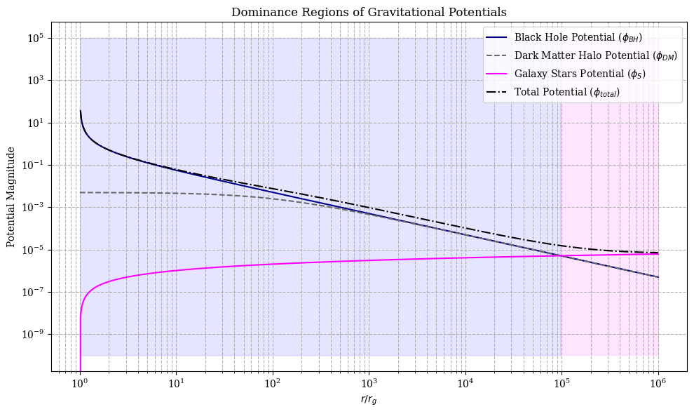
Figure 2: The magnitudes of the potentials for the black hole, dark matter halo, and galaxy stars are plotted at different length scales. The dot-dashed black line is their sum. Shaded regions are added to indicate where each potential dominates over the others. Blue shade for the black hole potential dominance. Red shade for the galaxy star potential dominance.

2.2 Gravitational Potential

To provide a more physical and accurate model of quasi-spherical accretion, we have applied a multi-component model of the Galactic potential. In cosmological simulations, the Bondi accretion rate is typically used to model the black hole’s gas accretion.

The total gravitational potential $\Phi$ is modeled as the sum of the potentials of the central black hole $\phi_{BH}$, the dark matter halo $\phi_{DM}$ and the stars of galaxy $\phi_{S}$ and can be expressed as

$$\Phi=\phi_{BH}+\phi_{DM}+\phi_{S}$$ (7)

This formulation allows us to systematically investigate how different components of the Galactic potential influence accretion dynamics over a wide range of scales. For the black hole potential, we consider the Paczyński–Wiita potential, which approximates the gravitational potential around a non-rotating black hole:

$$\phi_{BH}=-\frac{GM_{BH}}{r-r_{s}}$$ (8)

where $r$ is the radial distance from the black hole, $G$ is the gravitational constant, $M_{BH}$ is the mass of the black hole, and $r_{s}=2GM/c^{2}=2r_{g}$ is the Schwarzschild radius (with $c$ being the speed of light). This approach allows for the general relativistic effect in an approximate manner.

Around the Bondi radius, the effect of the gravitational potential will change compared to the case of a pure black hole potential. Such a change will potentially change the dynamics of accretion flow. So to study the accretion flow far away from the black hole, it is crucial to consider not only the gravitational potential of the black hole but also that of the galaxy stars and dark matter halo, as it plays a significant role and must be taken into account. The second term of Eq. 7 pertains to the potential of the dark matter halo, modeled using a Hernquist-type profile. The density distribution for this profile is given by:

$$\rho=\frac{M_{halo}a_{0}}{2\pi r(r+a_{0})^{3}}$$ (9)

where $M_{halo}$ is the total mass of the halo, and $a_{0}$ is a typical length scale. The potential of the dark halo, assumed to be spherical, is:

$$\phi_{DM}(r)=-\frac{GM_{halo}}{r+a_{0}}$$ (10)

where $G$ is the gravitational constant. This component becomes significant at larger scales, where the gravitational influence of the dark matter halo dominates over the black hole and stellar components.

The third term of Eq. 7 is the galaxy stars potential. Observations indicate a tight relation between the BH mass and the velocity dispersion of stars in the bulge (Ferrarese & Merritt (2000); Greene & Ho (2006)). Based on the $M_{BH}-\sigma$ correlation, it appears that the velocity dispersion of stars is a constant, which supports the idea that most AGNs exhibit a constant velocity dispersion (e.g. Kormendy & Ho (2013)). So the gravitational potential of the galaxy stars within the stars bulge is assumed to be (Bu et al. (2016))

$$\phi_{S}(r)=\sigma^{2}lnr+C$$ (11)

Where $C$ is a constant and $\sigma$ is the dispersion velocity of stars Bu et al. (2016), Sun & Yang (2021). It is common for elliptical galaxies with a central black hole mass $M_{BH}=10^{8}M_{\odot}$ to have a stellar dispersion velocity of $150-250$ $kms^{-1}$. We consider the dispersion velocity of stars to be a constant of radius, which is $\sigma=200km/s$ Kormendy & Ho (2013).

Then a question is how the above gravitational potential influence in a large value of $r$ can be in. Most numerical simulations of accretion flow so far have focused only on the region relatively close to the black, so it is difficult for them to answer this question. To answer it, we have to study the spherical accretion flow far away from the black hole, near the Bondi radius, or beyond the Bondi radius. In far from away distances, in addition to the potential of the black hole, the gravitational potential of the galaxy stars and dark matter halo will become important and should be included. Around the Bondi radius, the slope of the gravitational potential will change compared to the case of a pure black hole potential (see Figure 2). Such a change will potentially change the dynamics of accretion.

Figure 2 shows the magnitudes of the three potentials on the same graph to compare their values at different radii. Black Hole Potential Dominates at very small scales, close to the Schwarzschild radius. The gravitational influence is very strong near the event horizon and quickly diminishes with distance. Dark matter halo potential becomes significant at larger scales, reflecting the impact of the dark matter distribution in the galaxy. It remains relatively flat over a wide range of distances compared to the black hole potential. This potential represents the gravitational influence of the distribution of stars within the galaxy. It shows a more gradual change with distance, usually logarithmic, reflecting the spread of stellar mass. Highlight regions where each potential dominates. The blue shade indicates where the black hole potential is dominant and the red shade shows the the region where galaxy star potential is dominant.

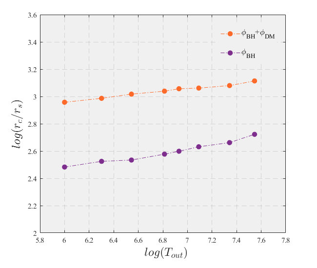
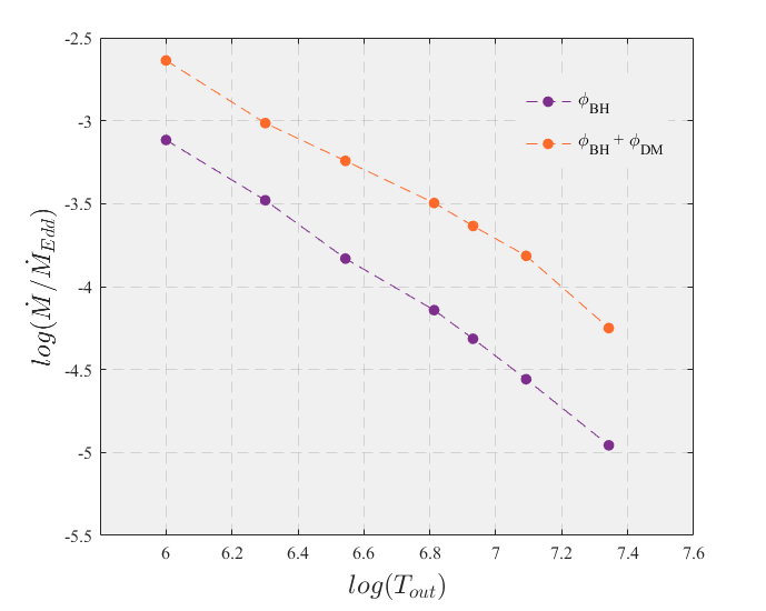
Figure 3: Left panel: The position of the critical point as a function of the temperature at the outer boundary $T_{out}$. Solutions are for $a_{0}=50,M_{halo}=M_{BH}$. Yellow dots are cases without dark matter potential and green dots are with dark matter potential. Right panel: Mass accretion rate with zero angular momentum in units of Eddington accretion rate as a function of temperature at the outer boundary ($T_{out}$), Our solution is for $a_{0}=50,M_{halo}=M_{BH}$. Magenta dots show the mass accretion rate without dark matter potential and green dots show the mass accretion rate with dark matter potential.

2.3 Numerical Method

Spherical accretion has a critical point, which prevents the direct integration of the equations from the outer subsonic region to the inner supersonic region. This difficulty has been handled in this way: either one starts with an arbitrarily chosen critical radius, integrates both inward and outward with the help of regularity conditions, and adjusts the critical radius until the outer and inner boundary conditions are satisfied. This approach ensures a smooth and physically consistent transition across the critical point. The governing differential equations are:

$$\frac{dc_{s}}{dr}=\frac{(\gamma-1)}{2vc_{s}}(-\frac{2vc_{s}^{2}}{r}-c_{s}^{2}\frac{dv}{dr})$$ (12)

$$\frac{dv}{dr}=\frac{v}{\gamma c_{s}^{2}-v^{2}}(\Omega_{k}^{2}r-\frac{2\gamma c_{s}^{2}}{r}+\frac{GM_{halo}}{(r+a)^{2}}+\frac{\sigma^{2}}{r})$$ (13)

The location of the sonic point is unknown and is an eigenvalue, so we need a three-boundary condition to solve equations.

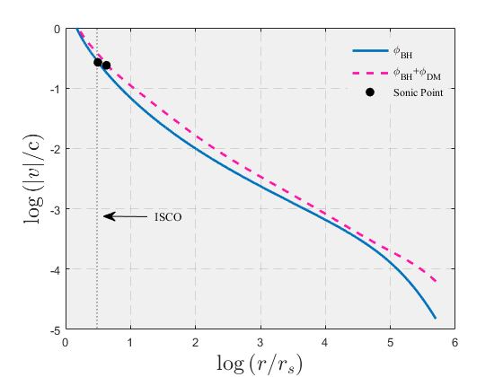
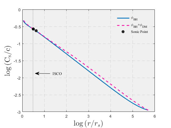
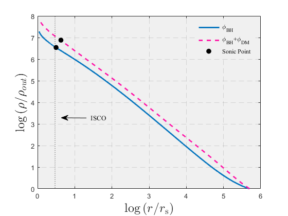
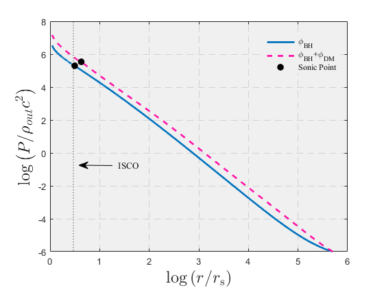
Figure 4: Global solutions for slowly rotating accretion flow,$L=85$, $\gamma=5/3$, $M_{halo}=M_{BH}$, $a=100$. Blue line related without dark matter potential,($\phi_{DM}=0,r_{c}=3.14$). Dashed pink curves ($\phi_{DM}\neq 0,r_{c}=4.25$). A solid dot indicates the position of the critical point. The vertical dotted lines correspond to the location of the marginally stable orbit (ISCO).

2.4 Boundary Condition

The dynamics of an astrophysical accretion flow can be characterized by a system of nonlinear ordinary differential equations. Consequently, the boundary condition assumes a potentially significant role in addressing this boundary value problem. Considering the inherent transonic nature of accretion onto a black hole, it is essential for the solution to fulfill the sonic-point condition at a distinct radius referred to as the sonic radius ($r_{c}$).

$$\frac{dv}{dr}=\frac{N}{D}$$ (14)

We have two boundary conditions in the sonic radius and one in the outer boundary. The boundary conditions at the sonic radius are as follows:

$$\gamma c_{s}^{2}-v^{2}=0,\quad r=r_{c}$$ (15)

$$\Omega_{k}^{2}r-\frac{2\gamma c_{s}^{2}}{r}+\frac{GM_{halo}}{(r+a)^{2}}+\frac{\sigma^{2}}{r}=0$$ (16)

These conditions ensure that the flow transitions smoothly through the sonic point, where the flow velocity equals the local sound speed. This transonic behavior is essential for realistic accretion models.

On the other hand, in complex astrophysical environments, the accreting gas at the outer boundary exhibits a variety of states, characterized by factors such as temperature and angular momentum. Consequently, an analysis of the accretion process necessitates consideration of the role played by the outer boundary condition (OBC). Such a model shows that the accretion power is as well coupled with the conditions in the outer gas as possible. At the outer boundary

$$c_{s}=c_{out}$$ (17)

In our study, we designate the Bondi radius as the outer boundary in our solutions that is $\sim 10^{5.7}$. While the classical Bondi model addresses accretion without angular momentum, real cosmic accretion invariably involves some rotation. Accounting for this rotation introduces additional complexity but provides a more realistic depiction of the process.

3 Low angular momentum accretion

The angular momentum of an accretion flow plays a crucial role in determining its flow characteristics. Low angular momentum accretion onto astrophysical black holes may manifest as practically inviscid flow in realistic astrophysical systems Olivares et al. (2023), such as detached binaries fueled by accretion from OB stellar winds Illarionov & Sunyaev (1975). Additionally, recent studies focusing on accretion onto the black hole at the center of our galaxy have also provided evidence for the existence of such flow Mościbrodzka et al. (2006), Moscibrodzka (2006). These flows represent an intermediate case between purely spherical accretion and disk accretion, making their study essential for understanding a wide range of astrophysical systems.

The governing equations for low angular momentum accretion are:

$$\frac{d}{dr}(4\pi\rho vr^{2})=0,$$ (18)

$$v\frac{dv}{dr}=r\Omega^{2}-\frac{d\Phi}{dr}-\frac{1}{\rho}\frac{dp}{dr}$$ (19)

$$v\frac{d}{dr}(\Omega r^{2})=\frac{1}{\rho r^{2}}(\rho\nu r^{4}\frac{d\Omega}{dr})$$ (20)

$$\frac{\rho v}{(\gamma-1)}\frac{dc_{s}^{2}}{dr}-c_{s}^{2}v\frac{d\rho}{dr}=\rho\nu r^{2}(\frac{d\Omega}{dr})^{2}$$ (21)

where $\nu$ is the kinematic coefficient of viscosity, which is defined by $\nu=\alpha c_{s}v$, the rotating accretion flow should have some viscosity that transports the angular momentum outward, thereby enabling the inward accretion of gas. $\Phi$ is the gravitational potential the same as eq 7 that included Paczynski–Wiita potential for the black hole, the potential of stars, and dark matter halo potential. To solve a differential equation in the subsonic region, we use a numerical technique similar to that described in Ranjbar & Abbassi (2023). For more details, please refer to the appendix. In the inner region, the differential equations are reduced to a set of linear algebraic equations that do not entail any boundary conditions at all. For the supersonic region, we have

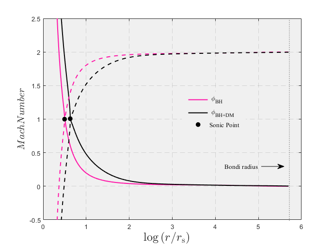
Figure 5: Global numerical solutions for the Mach Number. The pink line is for ($r_{c}=3.1447,a_{0}=0,M_{h}=0,\mathcal{L}=85$) and the black line ($r_{c}=4.2527,a_{0}=100,M_{h}=M_{BH},\mathcal{L}=85$). The position of the critical point located near the horizon of the black hole that shows with The solid black dot.

$$l_{in}=\Omega r^{2}$$ (22)

$$s_{in}=\frac{c_{s}^{2}}{\rho^{\gamma-1}}$$ (23)

$$B=\frac{v^{2}}{2}+\frac{l_{in}^{2}}{2r^{2}}+\Phi+\frac{\gamma s_{in}}{(\gamma-1)r^{2(\gamma-1)}v^{(\gamma-1})}(\frac{\dot{M}}{4\pi})^{(\gamma-1)}$$ (24)

where $l_{in}$ is the angular momentum per unit mass, $s_{in}$ is the entropy, and $B$ is the Bernoulli constant.

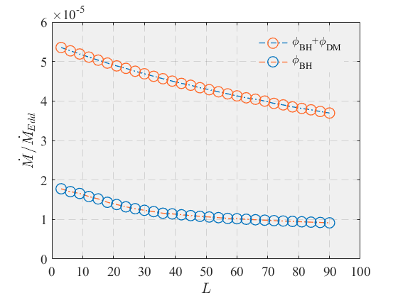
Figure 6: Mass accretion rate in units of Eddington accretion rate as a function of angular momentum at the outer boundary $\mathcal{L}>1$, The orange dots are for $a_{0}=100,M_{h}=M_{BH}$ and the blue line is the case without dark matter potential.

4 Numerical Results

This paper aims to obtain numerically exact global solutions for accretion flows with zero angular momentum and low angular momentum in the presence of a dark matter potential. Since self-similar solutions cannot describe flows in boundary regions, we utilized global solutions to understand the properties of the flow near the inner and outer boundaries. In this study, we employed the Hernquist profile to describe the spherical dark matter halo in elliptical galaxies. In this section, we present the results of our calculations and discuss their physical properties. We pay particular attention to the effects of including galaxy potential (DM + Stars) in the solutions. Our solutions in this study correspond to $a_{0}=50$ and $M_{halo}=M_{BH}$.

Table 1: Summary of Models

Model	Halo Gravity	Stars Gravity	$M_{\text{halo}}$	$a_{0}$	$L$	$T_{\text{out}}$	$\dot{M}_{\text{BH}}/\dot{M}_{\text{Edd}}$	$r_{c}/r_{s}$
Bondi	OFF	OFF	0	0	0	$6.5\times 10^{6}$	$7.21\times 10^{-5}$	386
Bondi	OFF	OFF	0	0	0	$1.0\times 10^{6}$	$7.65\times 10^{-4}$	304
Bondi	ON	ON	1	50	0	$6.5\times 10^{6}$	$5.12\times 10^{-4}$	1022
Bondi	ON	OFF	1	50	0	$6.5\times 10^{6}$	$3.19\times 10^{-4}$	1134
Bondi	ON	ON	1	100	0	$6.5\times 10^{6}$	$3.00\times 10^{-4}$	1253
SRAF	OFF	OFF	0	0	85	$6.5\times 10^{6}$	$9.30\times 10^{-6}$	3.20
SRAF	OFF	OFF	0	0	85	$1.0\times 10^{6}$	$2.01\times 10^{-4}$	3.02
SRAF	ON	OFF	1	50	85	$6.5\times 10^{6}$	$4.81\times 10^{-5}$	5.09
SRAF	ON	OFF	1	100	85	$6.5\times 10^{6}$	$3.75\times 10^{-5}$	4.11
SRAF	ON	OFF	1	100	85	$1.0\times 10^{6}$	$3.71\times 10^{-4}$	3.49

Table 2: Summary of Models, Col 1, the type of accretion flow. Cols 2 and 3 correspond to DM halo gravity and star gravity, and col 4 is the mass of the dark matter halo in units of the black hole mass. Col 5 is a characteristic scale length related to the dark matter halo. Cols 6 and 7, Specific angular momentum and temperature at the outer boundary. Col 8, the mass accretion rate normalized to the Eddington accretion rate. and col 9 the location of the sonic point normalized to the Schwarzschild radius $r_{s}$.

Figure 1 displays sample solutions, including the radial profiles of velocity, sound speed, density, and pressure corresponding to $\alpha=0.1$, $\gamma=5/3$, $c_{out}=10^{-3}$ and $\phi_{galaxy}=0$. The solutions clearly fall within the Bondi regime, as the gas exhibits negligible specific angular momentum at the outer boundary. The radial velocity is significant but remains lower than the near free-fall velocity characteristic of spherical Bondi flow. Notably, the angular momentum is zero for all solutions, truly representing Bondi accretion flow. The solution depicted by the upper curve in the four panels of Figure 1 ( $\phi_{DM}\neq 0$) provides clear evidence of the influence exerted by the gravitational potential of dark matter. The sonic radius, $r_{s}$, indicated by the black dot, is located at $417r_{g}$ without a dark matter halo and shifts to $745r_{g}$ when a dark matter halo is included. Figure 1 demonstrates the effect of the dark matter potential on Bondi accretion. In spherical accretion, the flow passes the critical point near the Bondi radius, becoming supersonic inside $r_{c}$.

Figure 3, the left panel illustrates the position of the sonic point as a function of temperature at the outer boundary, revealing systematic shifts as the dark matter potential is introduced. This figure shows how the sonic radius moves as we take into account dark matter potential. This behavior is particularly interesting as it highlights the influence of dark matter on the dynamics of accretion flows. Figure 3, the right panel shows the variation of the mass accretion rate as a function of temperature at the outer boundary. These temperatures are representative of the interstellar medium (ISM) in a galactic nucleus. It is evident that the addition of dark matter potential significantly increases the mass accretion rate.

However, in the case of rotating viscous accretion flow, a large portion of the flow remains subsonic well inside $r_{B}$ due to the rotational motion counterbalancing gravity. In figure 4 the critical radius $r_{c}$ for low angular momentum flow is much lower ($r_{c}\approx 3r_{s}$) compared to zero angular momentum flow. The sonic radius is close to the marginally stable orbit, $r_{ms}=3r_{g}$. As a result, when angular momentum is high, a sonic point will exist inside the ISCO radius; however, as angular momentum decreases, a sonic point may form outside the radius. The low angular momentum flow also exhibits a lower radial infall velocity at the outer boundary due to the reduced centrifugal force (Figure 1). These characteristics indicate that the low angular momentum flow more closely resembles spherical flow than disk flow, as expected.

Figure 5 depicts the radial profile of the Mach number, showing changes in its structure in the presence of a dark matter halo.␣‌Black dots show the position of the sonic point. These changes further underscore the impact of dark matter on the accretion flow dynamics.

Finally, Figure 6 presents the mass accretion rate in units of the Bondi rate as a function of angular momentum at the outer boundary, expressed in units of $L$. Our results indicate that, regardless of the value of $T_{\text{out}}$, the mass accretion rate $\dot{m}$ decreases as the rotation of the external gas $L$ increases, approaching the Bondi accretion rate as $L$ decreases. The mass accretion rate for the lowest angular momentum flow is nearly equal to the Bondi rate, while for the highest angular momentum flow, it is approximately 20 times smaller than the corresponding Bondi rate.

Table 2 compares different configurations of accretion models under various gravitational influences and parameters. The models include both Bondi and SRAF (Slowly rotating accretion flow) scenarios. Bondi Models: When both halo and star gravity are off, the accretion rate is the lowest ( $7.21\times 10^{-5}$ and the critical radius is $r_{g}$. Turning on star gravity (while keeping DM halo gravity off) increases the accretion rate slightly. When DM halo gravity is on (both with and without star gravity), the accretion rate significantly increases, and the critical radius also changes substantially. SRAF Models: Similar to the Bondi models, turning on halo gravity increases the accretion rate significantly. The presence of star gravity also affects the accretion rate but to a lesser extent compared to halo gravity.

Figure 8 illustrates the variation of the mass accretion rate as a function of $T_{\text{out}}$. This figure compares the accretion rate of the classical Bondi model with a modified model that incorporates the gravitational potential of the galaxy, dark matter potential, and rotation. At radii greater than $10\text{pc}$, the gravitational influence of the stars may surpass that of the black hole. The figure demonstrates that the inclusion of the galactic gravitational potential slightly enhances the mass accretion rate. Furthermore, the introduction of slow rotation to the Bondi model results in a decrease in the mass accretion rate compared to the classical Bondi rate.

Our models have made modifications to the classical Bondi model, as depicted in Figure 7. The figure illustrates the dependence of accretion rates on temperature at the outer boundary $T_{out}$. In Figure 7, the blue lines represent the accretion rates predicted by our model that normalize with Eddington accretion rate, while the red lines indicate $\dot{M}/\dot{M}_{Bondi}$. As shown in Fig. 7, with the increase of $T_{\text{out}}$, the accretion rates (blue lines) of our models decrease slower than the changing trend predicted by the Bondi model. Compared to our model, the Bondi model always overestimates the accretion rates, as shown by red lines. When turning on the effect of dark matter potential, the mass accretion rate is slightly strengthened. The gravitational potential is helpful to increase the accretion rates in our model.

These findings provide new insights into the behavior of accretion flows in the presence of dark matter, enhancing our understanding of the complex dynamics in galactic nuclei and the role of dark matter in influencing these processes.

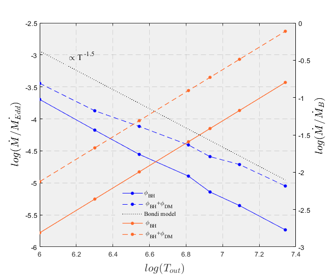
Figure 7: The dependence of accretion rates on the temperature at the outer boundary. We set the gas density at the outer boundary to be $10^{-24}grcm^{-3}$. Red lines mean the accretion rates $\dot{M}/\dot{M}_{Edd}$ predicted by our models while blue lines mean $\dot{M}/\dot{M}_{Bondi}$. Black dotted lines mean the changing trend of the accretion rates predicted by the Bondi model.

5 DISCUSSION AND SUMMARY

Given the extensive use of the classical Bondi theory, and considering that accretion on the MBHs at the center of galaxies is certainly more complicated than the description provided by this theory, the motivation for this work was to generalize the theory, including the effect of a general gravitational potential due to a host galaxy (stars + dark matter). In section 2 all the hypotheses of classical Bondi accretion (stationary, absence of rotation, spherical symmetry) were maintained. In section 3 we consider an accretion flow with slow rotation in the presence of galactic potential. The behavior of gases at the parsec scale can significantly impact the activity of low-luminosity active galactic nuclei (LLAGNs). In this study, we investigate the effect of dark matter on the properties of slightly rotating accretion flows around a non-rotating black hole. The model considered consists of a Schwarzschild black hole surrounded by dark matter, with a Bondi-like accretion flow. Initially, we consider spherically symmetric accretion flows at the outer boundary, introducing a small angular momentum to break the spherical symmetry. This study incorporates the Hernquist profile, a widely used model for dark matter halos, into the Bondi accretion scenario to examine its influence on the structure of the accretion flow. This approach allows us to systematically analyze how dark matter influences the structure and dynamics of accretion flows. The key difference between the present work and the previous ones is that we include the gravitational potential of the dark matter halo in addition to the black hole potential and galaxy potential at such large radii.

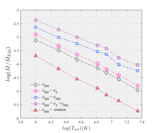
Figure 8: $M_{halo}=M_{BH}$, $a_{0}=50$, Variations of accretion rate as a function of temperature at the outer boundary in different gravitational potentials and rotation. Black diamond corresponds to the accretion model with zero angular momentum, Pink stars are the Bondi model with galaxy potential. Blue squares include dark matter potential. Violet circles are both of them. finally, red triangles show the accretion model with low angular momentum.

By introducing the dark matter potential, we aim to explore its impact on the dynamics of the accretion flow, including the effects of slight angular momentum. Our objective is to compare the influence of the dark matter halo on both spherical accretion and slowly rotating accretion flows, gaining insights into the distinct characteristics and consequences of these scenarios in the presence of a dark matter halo.

Our findings reveal significant differences between accretion flows with and without a dark matter halo. The presence of a dark matter halo affects the structure of accretion in the following ways:

1. The inclusion of the dark matter halo, combined with the black hole potential, leads to an increase in the mass accretion rate. Dark matter enhances the gravitational pull in the galaxy’s center, thereby increasing the mass accretion rate. The enhancement in accretion rates may also play a critical role in fueling LLAGNs, providing a pathway for interpreting observational data.

2. We found that the sonic point or sonic surface resides near the Bondi radius for low-angular momentum flows. The dark matter potential also affects the position of the sonic point. In both Bondi and slowly rotating accretion scenarios, the presence of dark matter significantly shifts the location of the sonic point. With increased temperature at the outer boundary, the sonic point or sonic surface can also be close to the Bondi radius.

3. When the black hole is embedded in a dark matter halo, our results indicate that dark matter effectively increases the mass accretion rate and expands the location of the sonic point in the non-rotating black hole.

Future investigations should explore additional profiles of dark matter halos, such as the NFW (Navarro-Frenk-White) and Jaffe profiles. By incorporating these different profiles into our analysis, we can further enhance our understanding of dark matter’s impact on the accretion process. Additionally, it would be valuable to examine the influence of a dark matter halo on outflow phenomena. Studying whether dark matter affects the intensity of outflows can provide critical insights into the complex relationship between dark matter and the overall dynamics of accretion processes. In this study, we assume that the couple between electrons and ions is sufficiently strong, resulting in a one-temperature plasma flow.

Appendix A Technical Method

The following section addresses the two-boundary value problem with unknown parameters, [$j,r_{\rm c}$]. Since the black hole accretion is necessarily transonic because of the nature of gravity around central objects, we define the critical point of the accretion flow in the following way. In principle, the critical point is a point of discontinuity of the differential equation and mathematically is defined as the $\mathrm{d}v/\mathrm{d}r\to 0/0$ form. Here, $r_{\rm c}$ denotes the location of the critical point. In the following subsection we try to simplify the system of the equation to be solved in a range $x=[r_{\rm c},x_{\rm out}]$.

A.1 System of BVP equations

The system of equations adopted in section 3 is written as:

$$\diff{v}{r}=f_{1r}=v\frac{\mathcal{N}}{\mathcal{D}},$$ (A1)

$$\diff{\Omega}{r}=f_{2r}=\frac{v\left(\Omega r^{2}-j\right)}{\alpha r^{3}c_{\mathrm{s}}},$$ (A2)

$$\diff{c_{\rm s}}{r}=f_{3r}=\frac{\gamma-1}{2vc_{\rm s}}\left[\frac{v^{2}\left(\Omega r^{2}-j\right)^{2}}{\alpha r^{3}c_{\rm s}}-\frac{2vc_{\rm s}^{2}}{r}-c_{\rm s}^{2}\diff{v}{r}\right],$$ (A3)

or equivalently,

$$f_{3r}=\frac{\gamma-1}{2vc_{\rm s}}\left[\frac{v^{2}\left(\Omega r^{2}-j\right)^{2}}{\alpha r^{3}c_{\rm s}}-\frac{2vc_{\rm s}^{2}}{r}-c_{\rm s}^{2}f_{1r}\right],$$ (A4)

where,

$$\mathcal{D} =\gamma c_{s}^{2}-v^{2},$$ (A5)

$$\mathcal{N} =\left(\Omega_{\mathrm{{}_{K}}}^{2}-\Omega^{2}\right)r-\frac{2\gamma c_{\rm s}^{2}}{r}$$

$$\quad+\frac{(\gamma-1)\left(\Omega r^{2}-j\right)^{2}v}{\alpha r^{3}c_{\rm s}}+\frac{GM_{halo}}{(r+a)^{2}}+\frac{\sigma^{2}}{r}.$$ (A6)

The Keplerian angular velocity is given by:

$$\Omega_{\mathrm{{}_{K}}}^{2}=\frac{GM}{r\left(r-r_{\mathrm{s}}\right)}.$$ (A7)

To determine the behavior of transonic solutions near the critical point, one needs to study $\left(\frac{\mathrm{d}v}{\mathrm{d}r}\right)_{\rm c}$. Since $\frac{\mathrm{d}v}{\mathrm{d}r}=\frac{N}{D}=\frac{0}{0}$ at a critical point, one must apply l’Hospital’s rule. Thus,

Since there is a singularity event near the horizon, we can not use the direct integration of hydrodynamics equations ( Runga-Kutta method ) from the outer boundary toward the horizon to obtain smooth global solutions. So we employ a powerful technique to solve this problem which is called the iterative relaxation technique Press et al. (1992). Although we can use a simpler shooting method since our computational domain for realistic external media is $r_{out}\sim parsec$, it’s better to use the relaxation method. Our problem is two two-point boundary values, which means we have no the value of variables in boundaries so we need to use the guess function. This method begins with a guess and as the solution is improved iteratively, the result tends to be the real solution In this method, $j$ and $r_{\rm c}$ are eigenvalues so consider an initial guess for them and then integrate from the outer boundary to the sonic radius. For the inner region, we have algebraic equations which it is easily solved. In our system, only one boundary abscissa $r_{\rm out}=x_{\rm max}$ is specified, while the other boundary $r_{\rm c}$ is to be determined.

A.2 Adding an extra constant dependent variable

In the above system, only one boundary abscissa $x_{\rm max}$ is specified, while the other boundary $r_{\rm c}$ is to be determined. Therefore, we add an extra constant dependent variable as Press et al. (1992),

$$y_{4}\equiv\ln(r_{\rm c})-\ln(x_{\rm max}),$$ (A8)

with the derivative:

$$\diff{y_{4}}{r}=0.$$ (A9)

We also define a new independent variable $t$ by setting,

$$\ln(x)-\ln(x_{\rm max})=ty_{4},\quad\quad 0\leq t\leq 1.$$ (A10)

Note here that we choose $\ln(x)$ since the outer boundary is very far from the inner boundary, i.e., $x_{\rm max}=r_{\mathrm{{}_{B}}}=10^{5.7}r_{\rm s}$.

A.3 Writing sys_bvp.m subroutine

The above system with a new independent variable, $t$, will be written as,

$$\diff{v}{t}=\diff{v}{\ln x}\diff{\ln x}{t}=f_{1}=xy_{4}*f_{1r},$$ (A11)

$$\diff{\Omega}{t}=f_{2}=xy_{4}*f_{2r},$$ (A12)

$$\diff{c_{\rm s}}{t}=f_{3}=xy_{4}*f_{3r},$$ (A13)

$$\diff{y_{4}}{t}=f_{4}=0,$$ (A14)

A.4 Boundary conditions

point $a$ is $r_{\rm out}$ and point $b$ shows the location of $r_{\rm c}$ which correspond to $t=0$ and $t=1$ respectively.

At $t=0$,

$$v_{a}=ya(1),\qquad\Omega_{a}=ya(2),\qquad c_{\rm sa}=ya(3),\\$$ (A15)

$$g(1)=\Omega_{a}-\frac{L}{0.136}(\frac{c}{c_{\mathrm{out}}})^{-4},\\$$ (A16)

$$g(2)=c_{\rm sa}-c_{\mathrm{out}}.\\$$ (A17)

At $t=1$,

$$v_{b}=yb(1),\qquad\Omega_{b}=yb(2),$$ (A18)

$$c_{\rm sb}=yb(3),\qquad y_{4}=yb(4),$$

$$r_{\rm c}=\exp(\ln(x_{\rm max})+y4)$$ (A19)

$$g(3) =\left(\Omega_{\rm Kb}^{2}-\Omega_{b}^{2}\right)r_{\rm c}-\frac{2\gamma c_{\rm sb}^{2}}{r_{\rm c}},$$ (A20)

$$\quad+\frac{(\gamma-1)(\Omega_{b}r_{c}^{2}-j)^{2}v_{b}}{\alpha r_{c}^{3}c_{\rm sb}}+\frac{GM_{h}}{(r_{\rm c}+a)^{2}}+\frac{\sigma^{2}}{r_{\rm c}},$$

$$g(4)=\gamma c_{\rm sb}^{2}-v_{b}^{2},$$ (A22)

$$g(5)=\Omega_{b}r_{c}^{2}-j+\frac{2\alpha c_{\rm sb}\Omega_{b}r_{c}^{2}}{v_{b}}.$$ (A23)

References

- Barai et al. (2011) Barai, P., Proga, D., & Nagamine, K. 2011, MNRAS, 418, 591, doi: 10.1111/j.1365-2966.2011.19508.x
- Bondi (1952) Bondi, H. 1952, Monthly Notices of the Royal Astronomical Society, 112, 195, doi: 10.1093/mnras/112.2.195
- Bu et al. (2016) Bu, D.-F., Yuan, F., Gan, Z.-M., & Yang, X.-H. 2016, ApJ, 818, 83, doi: 10.3847/0004-637X/818/1/83
- Cardoso et al. (2022) Cardoso, V., Dias, O. J. C., et al. 2022, Physical Review D, 105, 061501, doi: 10.1103/PhysRevD.105.f1501
- Ciotti & Pellegrini (2017) Ciotti, L., & Pellegrini, S. 2017, ApJ, 848, 29, doi: 10.3847/1538-4357/aa8d1f
- Ciotti & Pellegrini (2018) —. 2018, ApJ, 868, 91, doi: 10.3847/1538-4357/aae97d
- Ferrarese & Merritt (2000) Ferrarese, L., & Merritt, D. 2000, ApJ, 539, L9, doi: 10.1086/312838
- Gavazzi et al. (2007) Gavazzi, R., Treu, T., Rhodes, J. D., et al. 2007, ApJ, 667, 176, doi: 10.1086/519237
- Greene & Ho (2006) Greene, J. E., & Ho, L. C. 2006, ApJ, 641, 117, doi: 10.1086/500353
- Hernquist (1990) Hernquist, L. 1990, The Astrophysical Journal, 356, 359, doi: 10.1086/168785
- Hopkins et al. (2008) Hopkins, P. F., Hernquist, L., Cox, T. J., & Kereš, D. 2008, ApJS, 175, 356, doi: 10.1086/524362
- Illarionov & Sunyaev (1975) Illarionov, A. F., & Sunyaev, R. A. 1975, A&A, 39, 185
- Jaffe (1983) Jaffe, W. 1983, Monthly Notices of the Royal Astronomical Society, 202, 995, doi: 10.1093/mnras/202.4.995
- King (1962) King, I. 1962, The Astronomical Journal, 67, 471, doi: 10.1086/108754
- Kormendy & Ho (2013) Kormendy, J., & Ho, L. C. 2013, Annual Review of Astronomy and Astrophysics, 51, 511, doi: 10.1146/annurev-astro-082812-140018
- Korol et al. (2016) Korol, V., Ciotti, L., & Pellegrini, S. 2016, MNRAS, 460, 1188, doi: 10.1093/mnras/stw1029
- Moscibrodzka (2006) Moscibrodzka, M. 2006, A&A, 450, 93, doi: 10.1051/0004-6361:20054165
- Mościbrodzka et al. (2006) Mościbrodzka, M., Das, T. K., & Czerny, B. 2006, MNRAS, 370, 219, doi: 10.1111/j.1365-2966.2006.10470.x
- Narayan & Fabian (2011) Narayan, R., & Fabian, A. C. 2011, MNRAS, 415, 3721, doi: 10.1111/j.1365-2966.2011.18987.x
- Navarro et al. (1996) Navarro, J. F., Frenk, C. S., & White, S. D. M. 1996, The Astrophysical Journal, 462, 563, doi: 10.1086/177394
- Olivares et al. (2023) Olivares, H. R., Mościbrodzka, M. A., & Porth, O. 2023, Astronomy & Astrophysics, 678, doi: 10.1051/0004-6361/202247253
- Philipp et al. (1999) Philipp, S., Zylka, R., Mezger, P. G., et al. 1999, Astronomy and Astrophysics, 348, 768
- Press et al. (1992) Press, W. H., Teukolsky, S. A., Vetterling, W. T., & Flannery, B. P. 1992, Numerical Recipes in FORTRAN 77: The Art of Scientific Computing, 2nd edn. (Cambridge, UK: Cambridge University Press)
- Ranjbar & Abbassi (2023) Ranjbar, R., & Abbassi, S. 2023, The Astrophysical Journal, 954, 117, doi: 10.3847/1538-4357/ace163
- Ricotti (2007) Ricotti, M. 2007, The Astrophysical Journal, 662, 53, doi: 10.1086/512364
- Samadi et al. (2019) Samadi, M., Zanganeh, S., & Abbassi, S. 2019, MNRAS, 489, 3870, doi: 10.1093/mnras/stz2397
- Sun & Yang (2021) Sun, H.-W., & Yang, X.-H. 2021, MNRAS, 505, 4129, doi: 10.1093/mnras/stab1616
- Tremaine et al. (2002) Tremaine, S., Gebhardt, K., Bender, R., et al. 2002, ApJ, 574, 740, doi: 10.1086/341002
- Treu & Koopmans (2002) Treu, T., & Koopmans, L. V. E. 2002, ApJ, 575, 87, doi: 10.1086/341216
- Treu & Koopmans (2004) —. 2004, ApJ, 611, 739, doi: 10.1086/422245
- Yang & Bu (2018) Yang, X.-H., & Bu, D.-F. 2018, MNRAS, 478, 2887, doi: 10.1093/mnras/sty1254