How to Upscale Neural Networks with Scaling Law?
A Survey and Practical Guidelines

Abstract

Neural scaling laws have revolutionized the design and optimization of large-scale AI models by revealing predictable relationships between model size, dataset volume, and computational resources. Early research established power-law relationships in model performance, leading to compute-optimal scaling strategies. However, recent studies highlighted their limitations across architectures, modalities, and deployment contexts. Sparse models, mixture-of-experts, retrieval-augmented learning, and multimodal models often deviate from traditional scaling patterns. Moreover, scaling behaviors vary across domains such as vision, reinforcement learning, and fine-tuning, underscoring the need for more nuanced approaches. In this survey, we synthesize insights from over 50 studies, examining the theoretical foundations, empirical findings, and practical implications of scaling laws. We also explore key challenges, including data efficiency, inference scaling, and architecture-specific constraints, advocating for adaptive scaling strategies tailored to real-world applications. We suggest that while scaling laws provide a useful guide, they do not always generalize across all architectures and training strategies.

How to Upscale Neural Networks with Scaling Law?
A Survey and Practical Guidelines

Ayan Sengupta^∗  Yash Goel^∗  Tanmoy Chakraborty Indian Institute of Technology Delhi, India {ayan.sengupta, ee1210984, tanchak}@ee.iitd.ac.in

^*

1 Introduction

Scaling laws have become a fundamental aspect of modern AI development, especially for large language models (LLMs). In recent years, researchers have identified consistent relationships between model size, dataset volume, and computational resources, demonstrating that increasing these factors leads to systematic improvements in performance. These empirical patterns have been formalized into mathematical principles, known as scaling laws, which provide a framework for understanding how the capabilities of neural networks evolve as they grow. Mastering these laws is crucial for building more powerful AI models, optimizing efficiency, reducing costs, and improving generalization.

The study of neural scaling laws gained prominence with the foundational work of Kaplan et al. (2020), who demonstrated that model performance follows a power-law relationship with respect to size, data, and compute. Their findings suggested that larger language models (LMs) achieve lower loss when trained on sufficiently large datasets with increased computational resources. Later, Hoffmann et al. (2022) refined these ideas, introducing the notion of compute-optimal scaling, which revealed that training a moderate-sized model on a larger dataset is often more effective than scaling model size alone. However, recent studies Muennighoff et al. (2023); Caballero et al. (2023); Krajewski et al. (2024) have challenged the universality of these laws, highlighting cases where sparse models, mixture-of-experts architectures, and retrieval-augmented methods introduce deviations from traditional scaling patterns. These findings suggested that while scaling laws provide a useful guide, they do not always generalize across all architectures and training strategies.

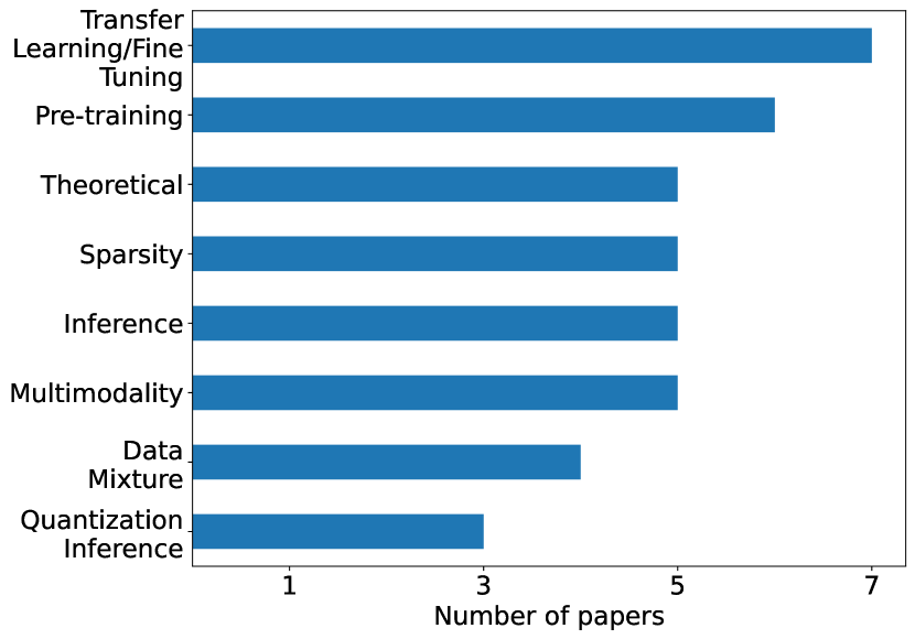
Figure 1: Papers surveyed under different categories. The detailed paper list is provided in Table 6 of Appendix B.

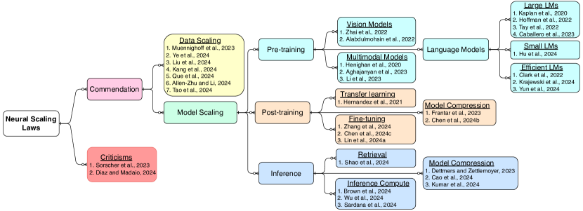
Figure 2: A taxonomy of neural scaling laws.

Despite the growing importance of scaling laws, existing research remains fragmented, with limited synthesis of theoretical foundations, empirical findings, and practical implications. Given the rapid evolution of this field, there is a need for a structured analysis that consolidates key insights, identifies limitations, and outlines future research directions. While theoretical studies have established the mathematical principles governing scaling, their real-world applications, such as efficient model training, optimized resource allocation, and improved inference strategies, are less explored. To address this gap, we reviewed over 50 research articles (Figure 1 highlights papers on scaling laws on different topics) to comprehensively analyze scaling laws, examining their validity across different domains and architectures.

While prior surveys have made valuable contributions to understanding scaling laws, they have primarily focused on specific aspects of the scaling phenomenon (See Table 1). Choshen et al. (2024) emphasized statistical best practices for estimating and interpreting scaling laws using training data, while Li et al. (2024b) emphasized on methodological inconsistencies in scaling studies and the reproduction crisis in scaling laws. Our survey distinguishes itself by offering comprehensive coverage of architectural considerations, data scaling implications, and inference scaling – areas that previous surveys either overlooked or addressed only partially.

Category	Choshen et al. (2024)	Li et al. (2024b)	Ours
Covers neural scaling laws broadly	Yes	No	Yes
Discusses fitting methodologies	Yes	Yes	Yes
Analyzes architectural considerations	No	Limited	Yes
Includes data scaling and pruning	No	Limited	Yes
Explores inference scaling	No	Limited	Yes
Considers domain-specific scaling	No	No	Yes
Provides practical guidelines	Yes	Yes	Yes
Critiques limitations of scaling laws	Limited	Yes	Yes
Proposes future research directions	Limited	Yes	Yes

Table 1: Key differences between our survey and existing surveys on neural scaling laws (Choshen et al., 2024; Li et al., 2024b).

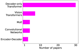
(a) Architecture-wise statistics

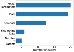
(b) Variable-wise statistics

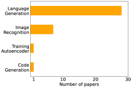
(c) Task-wise statistics

Figure 3: Number of paper studied in this survey paper for different model architectures (a), scaling variables (b) and scaling tasks (c). The detailed paper list is provided in Table 6 of Appendix B.

2 Taxonomy of neural scaling laws

Understanding the scaling laws of neural models is crucial for optimizing performance across different domains. We predominantly explore the scaling principles for language models, extending to other modalities such as vision and multimodal learning. We also examine scaling behaviors in domain adaptation, inference, efficient model architectures, and data utilization. We highlight the taxonomy tree of scaling laws research in Figure 2. As highlighted in Figure 1, neural scaling laws have been proposed predominantly for pre-training and fine-tuning scaling of large neural models. Among the models studied, as highlighted in Figure 3a, decoder-only Transformers dominate the subject, followed by vision transformers (ViT) and Mixture-of-Experts (MoE).

The most common neural scaling laws take the form of power laws (Equation 1), where the model’s loss ($L$) or performance metric assumes to follow a predictable relationship with different scaling variables,

$$L(P_{i....n})=\sum_{i=1}^{n}\alpha_{i}\cdot P_{i}^{-\beta_{i}}$$ (1)

with appropriate scaling parameters $\beta_{i}$ and fitting parameters $\alpha_{i}$ for different scaling parameter $P_{i}$. Figure 3b highlights that the number of model parameters and data size are the most common used scaling factors. The exact forms of all the scaling laws are highlighted in Table 7 of Appendix B. Among all the tasks, Figure 3c suggests that language generation is the most common task used for developing these scaling laws, where the training cross-entropy loss is widely used to fit the laws. Based on the values obtained empirically, the scaling laws are fitted with non-linear optimization, most commonly by running algorithms like least square and BFGS (Broyden-Fletcher-Goldfarb-Shanno). Statistical methods like goodness-of-fit metrics are used to validate the correctness of the fitted curves. We elaborate on the evaluation of neural scaling laws in Appendix A.

In the following sections, we review the existing literature on neural scaling across various domains.

2.1 Scaling laws of language models

Kaplan et al. (2020) suggested that larger LMs improve performance by reducing loss through power-law scaling. However, this view evolved when studies showed that many large models were undertrained, and data scaling plays an equally crucial role in compute efficiency (Hoffmann et al., 2022). More recent breakthroughs challenged traditional scaling assumptions. Broken Neural Scaling Law (BNSL) introduced non-monotonic trends, meaning that model performance can sometimes worsen before improving, depending on dataset thresholds and architectural bottlenecks (Caballero et al., 2023). Another exciting development came from small LMs, where optimized training strategies, such as a higher data-to-parameter ratio and adaptive learning schedules, enable models ranging from 1.2B to 2.4B parameters to rival significantly larger 7B-13B models (Hu et al., 2024). These findings reshape the fundamental assumptions of scaling laws, proving that strategic training can outperform brute-force model expansion.

Modality	Paper	Key insights	Applicability
Language	Kaplan et al. (2020)	Larger models are more sample-efficient, needing fewer training examples to generalize well.	Predicts model loss decreases with increasing parameters, used in early LMs like GPT-3.
2-4	Hoffmann et al. (2022)	The best performance comes from balancing model size and data, rather than just increasing parameters.	Balances compute, model size, and dataset size for optimal efficiency, as seen in Chinchilla.
2-4	Caballero et al. (2023)	Performance does not always improve smoothly; there are inflection points where scaling stops working.	Identifies phase transitions, minimum data thresholds, and unpredictability in scaling behavior.
2-4	Hu et al. (2024)	Smaller models with better training can rival much larger models.	Demonstrates that smaller models with optimized training can outperform larger undertrained models.
Vision	Zhai et al. (2022)	ViTs follow power-law scaling but plateau at extreme compute levels, with benefits primarily seen in datasets >1B images.	Image classification, object detection, large-scale vision datasets.
Multimodal	Aghajanyan et al. (2023)	Multimodal models experience competition at smaller scales but transition into synergy as model and token count grow.	Multimodal learning, mixed-modal generative models, cross-domain AI.
2-4	Li et al. (2024a)	Scaling vision encoders in vision-language models does not always improve performance, reinforcing the importance of data quality over raw scaling.	Vision-language models, image-text alignment, multimodal scaling challenges.

Table 2: Critical neural scaling laws for language, vision and multimodal models.

2.2 Scaling laws in other modalities

In computer vision, ViTs exhibit power-law scaling when model size, compute, and data grow together, but their performance plateaus at extreme compute levels, with noticeable gains only when trained on datasets exceeding 1B images (Zhai et al., 2022). Meanwhile, studies on scaling law extrapolation revealed that while larger models generally scale better, their efficiency declines at extreme sizes, requiring new training strategies to maintain performance (Alabdulmohsin et al., 2022). In multimodal learning, an interesting phenomenon called the “competition barrier” has been observed where at smaller scales different input modalities compete for model capacity, but as models grow, they shift into a synergistic state, enabling accurate performance predictions based on model size and token count (Aghajanyan et al., 2023).

However, not all scaling trends align with expectations. Contrary to the assumption that larger is always better, scaling vision encoders in vision-language models can sometimes degrade performance, highlighting the fact that data quality and modality alignment are more critical than brute-force scaling (Li et al., 2024a). These findings collectively emphasize that scaling laws are domain-dependent – optimal scaling strategies require a careful balance between compute efficiency, dataset quality, and architecture rather than simply increasing model size. Table 2 summarizes the scaling laws of pre-trained models for language and other modalities.

2.3 Scaling laws for domain adaptation

Pre-training and fine-tuning techniques have accelerated the adoption of large-scale neural models, yet the extent to which these models transfer across tasks and domains remains a key research question tied to scaling principles. Studies show that transfer learning follows a power-law where pre-training amplifies fine-tuning effectiveness, especially in small data regimes. Even with limited downstream data, larger models benefit significantly from pre-training, improving generalization (Hernandez et al., 2021). In vision, pre-training saturation occurs due to upstream-downstream interactions, rather than just task complexity. Lower network layers quickly specialize in simple tasks, while higher layers adapt to complex downstream objectives (Abnar et al., 2021). Similarly, in synthetic-to-real transfer, larger models consistently reduce transfer gaps, enhancing generalization across domains (Mikami et al., 2021).

Fine-tuning strategies scale differently depending on dataset size. Parameter-efficient fine-tuning (PEFT) is well-suited for small datasets, low-rank adaptation (LoRA) (Hu et al., 2021) performs best for mid-sized datasets, and full fine-tuning is most effective for large datasets. However, PEFT methods provide better generalization in large models, making them attractive alternatives to full-scale fine-tuning (Zhang et al., 2024).

Scaling laws are also being utilized to accurately predict the fine-tuning performance of models. The FLP method (Chen et al., 2024c) estimates pre-training loss from FLOPs, enabling accurate forecasts of downstream performance, particularly in models up to 13B parameters. Further refinements like FLP-M improve mixed-dataset predictions and better capture emergent abilities in large models. Finally, the Rectified scaling law (Lin et al., 2024a) introduces a two-phase fine-tuning transition, where early-stage adaptation is slow before shifting into a power-law improvement phase. This discovery enables compute-efficient model selection using the “Accept then Stop” (AtS) algorithm to terminate training at optimal points.

Paper	Key insights	Applicability
Hernandez et al. (2021)	Pre-training amplifies fine-tuning, particularly for small datasets, and benefits larger models even under data constraints.	Transfer learning, pre-training optimization, few-shot learning.
1-3 Abnar et al. (2021)	Large-scale pre-training improves downstream performance, but effectiveness depends on upstream-downstream interactions, not task complexity.	Vision transfer learning, upstream-downstream performance interactions.
1-3 Zhang et al. (2024)	Optimal fine-tuning strategy depends on dataset size: PEFT for small, LoRA for mid-scale, and full fine-tuning for large-scale datasets.	Fine-tuning strategies, parameter-efficient tuning, LoRA, full fine-tuning.
1-3 Lin et al. (2024a)	Fine-tuning follows a two-phase transition: slow early adaptation followed by power-law improvements, guiding compute-efficient model selection.	Compute-efficient fine-tuning, early stopping, model selection strategies.

Table 3: Key highlights from scaling of fine-tuned and domain-adapted models.

We summarize these findings in Table 3, suggesting that transfer learning is highly scalable, but effective scaling requires precise tuning strategies rather than just increasing model size.

2.4 Scaling laws for model inference

Simply scaling up models is not always the best way to improve model performance.  Chen et al. (2024a) suggested that more efficient test-time compute strategies can dramatically reduce inference costs while maintaining or even exceeding performance. Instead of blindly increasing LLM calls, they further suggested for allocating resources based on query complexity, ensuring that harder queries receive more compute while simpler ones use fewer resources. The importance of test-time compute strategies becomes even clearer when dealing with complex reasoning tasks. While sequential modifications work well for simple queries, parallel sampling and tree search dramatically improve results on harder tasks. Adaptive compute-optimal techniques have been shown to reduce computational costs by 4$\times$ without degrading performance, allowing smaller models with optimized inference strategies to surpass much larger models (Snell et al., 2024; Brown et al., 2024). Advanced inference approaches, such as REBASE tree search (Wu et al., 2024), further push the boundaries of efficiency, enabling small models to perform on par with significantly larger ones.

Another breakthrough came from retrieval augmented models, where increasing the datastore size consistently improves performance without hitting saturation (Shao et al., 2024). This allows smaller models to outperform much larger ones on knowledge-intensive tasks, reinforcing that external datastores provide a more efficient alternative to memorizing information in model parameters.

Paper	Key insights	Applicability
Brown et al. (2024)	Adaptive test-time compute strategies reduce computational costs by 4$\times$ while maintaining performance, enabling smaller models to compete with much larger ones.	Test-time compute efficiency, inference cost reduction, compute-limited environments.
1-3 Wu et al. (2024)	Advanced inference methods like REBASE tree search allow smaller models to match the performance of significantly larger ones.	High-efficiency inference, performance optimization for small models.
1-3 Shao et al. (2024)	Increasing datastore size in retrieval-augmented models consistently improves performance under the same compute budget, without evident saturation.	Retrieval-augmented language models, knowledge-intensive tasks, compute-efficient architectures.
1-3 Clark et al. (2022)	Routing-based models show diminishing returns at larger scales, requiring optimal routing strategies for efficiency.	Routing-based models, MoEs, transformer scaling.
1-3 Krajewski et al. (2024)	Fine-grained MoEs achieve up to 40$\times$ compute efficiency gains when expert granularity is optimized.	Mixture of Experts models, large-scale compute efficiency.
1-3 Frantar et al. (2023)	Sparse model scaling enables predicting optimal sparsity levels for given compute budgets.	Sparse models, structured sparsity optimization, parameter reduction.

Table 4: Scaling laws of efficient models.

2.5 Scaling laws for efficient models

Scaling laws have expanded beyond simple parameter growth, introducing new methods to optimize routing, sparsity, pruning, and quantization for efficient LLM scaling. Routing-based models benefit from optimized expert selection, but their returns diminish at extreme scales, requiring careful expert configuration (Clark et al., 2022). In contrast, fine-grained MoE models consistently outperform dense transformers, achieving up to 40$\times$ compute efficiency gains when expert granularity is properly tuned (Krajewski et al., 2024). However, balancing the number of experts ($E$) is crucial, where models with 4-8 experts offer superior inference efficiency, but require $2.5-3.5\times$ more training resources, making 16-32 expert models more practical when combined with extensive training data (Yun et al., 2024). Sparse model scaling offers another efficiency boost. Research has demonstrated that higher sparsity enables effective model scaling, allowing $2.15\times$ more parameters at 75% sparsity, improving training efficiency while maintaining performance (Frantar et al., 2023). Additionally, pruning laws ($\text{P}^{2}$ scaling laws) predict that excessive post-training data does not always improve performance, helping optimize resource allocation in pruned models (Chen et al., 2024b). Dettmers and Zettlemoyer (2023) showed that 4-bit quantization provides the best trade-off between accuracy and model size, optimizing zero-shot performance while reducing storage costs. Larger models tolerate lower precision better, following an exponential scaling law where fewer high-precision components are needed to retain performance (Cao et al., 2024). Meanwhile, training precision scales logarithmically with compute budgets, with 7-8 bits being optimal for balancing size, accuracy, and efficiency (Kumar et al., 2024). Recent reserach has expanded into distillation as well, developing a mathematical framework that predicts how well a student model will perform based on the student model’s size, the teacher model’s performance and the compute budget allocation between the teacher and the student (Busbridge et al., 2025). We summarize these practical insights in Table 4 for better readability.

2.6 Data scaling laws

Paper	Key insights	Applicability
Ye et al. (2024)	Predicts optimal data compositions before training, reducing compute costs by up to 27% while maintaining performance.	Pre-training optimization, data efficiency improvements.
1-3 Liu et al. (2024)	REGMIX optimizes data mixtures using proxy models, achieving 90% compute savings.	Compute-efficient training, automated data selection, large-scale models.
1-3 Allen-Zhu and Li (2024)	Language models can store 2 bits of knowledge per parameter, with knowledge retention dependent on training exposure.	Knowledge encoding, model compression, retrieval-augmented models.

Table 5: Critical scaling laws for data mixing and knowledge capacity.

Scaling models involves more than just increasing parameters; optimizing data mixtures, training duration, and vocabulary size also plays a crucial role in enhancing performance and efficiency. Data mixing laws allow AI practitioners to accurately predict optimal data compositions before training, leading to 27% fewer training steps without compromising accuracy (Ye et al., 2024). Techniques like REGMIX optimize data selection using proxy models and regression, reducing compute costs by 90% compared to manual data selection (Liu et al., 2024). Meanwhile, AUTOSCALE revealed that data efficiency depends on model scale, where high-quality data like Wikipedia helps small models but loses effectiveness for larger models, which benefit from diverse datasets like CommonCrawl (Kang et al., 2024). For continual learning, the D-CPT Law provided a theoretical framework for balancing general and domain-specific data, guiding efficient domain adaptation and long-term model updates (Que et al., 2024). Additionally, Chinchilla scaling assumptions were challenged by evidence showing that training models for more epochs on limited data can outperform simply increasing model size (Muennighoff et al., 2023). Repeated data exposure remains stable up to 4 epochs, but returns diminish to zero after around 16 epochs, making longer training a more effective allocation of compute resources. Furthermore, the vocabulary scaling law suggested that as language models grow larger, their optimal vocabulary size should increase according to a power law relationship (Tao et al., 2024). Finally, knowledge capacity scaling laws established that language models store 2 bits of knowledge per parameter, meaning a 7B model can encode 14B bits of knowledge – surpassing English Wikipedia and textbooks combined (Allen-Zhu and Li, 2024). Table 5 summarizes the data scaling laws for developing neural models when data is not available in abundance.

3 Practical guidelines for utilizing scaling laws

Large-scale adoption of neural models requires careful determination of several key factors:

• Model size vs. data size: How should the number of parameters and dataset size be balanced to achieve optimal performance?

• Compute budget: Given a fixed computational budget, how can training and inference be optimized for efficiency?

• Training strategy: Should longer training duration be prioritized over increased model size, especially in data-constrained environments?

• Architecture choice: Should the model be dense or sparse (e.g., MoE) to optimize performance for a given budget?

• Inference efficiency: What test-time strategies, such as retrieval augmentation or tree search, can be employed to enhance model output quality?

• Quantization and pruning: How can quantization and structured sparsity be used to minimize memory footprint while maintaining accuracy?

Based on the selections of the above choices, one can follow the steps highlighted in Figure 4 for developing large-scale neural models. Figure 4a illustrates that for developing large-scale models with multimodal capabilities, multimodal scaling laws Aghajanyan et al. (2023) can be followed. For developing domain-specific nuanced application, one can follow D-CPT law Que et al. (2024), which provides a comprehensive guideline for domain-continuous pre-training. For developing general-purpose LLMs, one may need to follow Kaplan/Chinchilla scaling laws, if sufficient data is available and the model choice is dense; otherwise, MoE scaling laws Krajewski et al. (2024) be utilized to develop sparser models. If sufficient data is not available, one can either train the model for longer epochs, following Sardana et al. (2024), or use data mixing strategies Ye et al. (2024) for deriving optimal data composition for pre-training the model.

Post-training, inference strategies (c.f. Figure 4b) can be followed to ensure that the model is utilized efficiently for the downstream applications. If the high memory consumption of the model is a concern, compression strategies like pruning Chen et al. (2024b) or low-precision quantization Cao et al. (2024) can be used. To make larger models inference efficient, inference scaling laws Wu et al. (2024) or test-time scaling laws Chen et al. (2024a) can be utilized. Appendix D elaborates more practical guidelines in terms of using the existing literature of neural scaling laws for developing large-scale neural models.

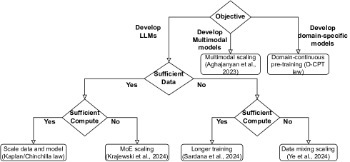
(a) Training strategies

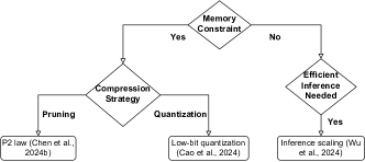
(b) Inference strategies

Figure 4: Practical guidelines for utilizing neural scaling laws while developing large-scale models.

4 Criticisms of scaling laws

Diaz and Madaio (2024) challenged the generalizability of neural scaling laws, arguing that they fail in diverse real-world AI applications. They argued that scaling laws do not always hold when AI models serve heterogeneous populations with conflicting criteria for model performance. Larger datasets inherently reflect diverse communities, making it difficult to optimize a single model for all users. Similar to issues in multilingual AI, increasing data diversity often leads to performance degradation rather than improvement. Universal evaluation metrics are inadequate for capturing these complexities, potentially reinforcing biases against underrepresented groups. The authors further argued that smaller, localized AI models may be more effective for specific communities, highlighting the need to move beyond one-size-fits-all scaling assumptions.

Beyond dataset expansion, data pruning contradicts traditional scaling laws by demonstrating that performance improvements do not always require exponentially more data. Strategic pruning achieves comparable or superior results with significantly fewer training samples (Sorscher et al., 2023). Not all data contributes equally, and selecting the most informative examples enables more efficient learning. Experimental validation on CIFAR-10, SVHN, and ImageNet shows that careful dataset curation can surpass traditional power-law improvements, questioning the necessity of brute-force scaling.

Despite their significant impact, many studies on scaling laws suffer from limited reproducibility (see Table 8 in Appendix C) due to proprietary datasets, undisclosed hyperparameters, and undocumented training methodologies. The inability to replicate results across different computing environments raises concerns about their robustness. Large-scale experiments conducted by industry labs often depend on private infrastructure, making independent verification challenging. This lack of transparency undermines the reliability of scaling law claims and highlights the urgent need for open benchmarks and standardized evaluation frameworks to ensure reproducibility.

5 Future recommendations

While neural scaling laws have provided valuable insights into model performance, their current formulations often fail to account for recent advancements in architecture, data efficiency, and inference strategies. The following directions highlight key areas where scaling laws should be adapted to improve their predictive power and practical utility.

Inference-aware scaling: Scaling laws should incorporate test-time computation, as compute-efficient inference strategies (e.g., iterative refinement, tree search, retrieval-based augmentation) can allow smaller models to outperform larger ones. Future research should focus on balancing training vs. inference compute costs to develop models that scale efficiently in real-world applications.

Compute-optimal model selection: Scaling laws should not only predict performance improvements but also guide model selection given a fixed compute budget. Future work should explore multi-objective optimization frameworks that balance performance, energy efficiency, and cost to drive more sustainable AI development.

Efficient data scaling and pruning: The optimization of model scaling necessitates a shift from volume-based to quality-focused data selection. Future frameworks should prioritize informative examples and integrate diversity metrics to enhance generalization, moving beyond simple dataset expansion.

6 Conclusion

This survey provided a comprehensive analysis of neural scaling laws, exploring their theoretical foundations, empirical findings, and practical implications. It synthesized insights across various modalities, including language, vision, multimodal learning, and reinforcement learning, to uncover common trends and deviations from traditional power-law scaling. While early research established predictable relationships between model size, dataset volume, and computational resources, more recent studies have shown that these relationships are not universally applicable. Sparse architectures, retrieval-augmented models, and domain-specific adaptations often exhibit distinct scaling behaviors, challenging the notion of uniform scalability. Furthermore, advancements in fine-tuning, data pruning, and efficient inference strategies have introduced new perspectives on compute-optimal scaling. Despite their significance, scaling laws remain an evolving area of research, requiring further refinement to address real-world deployment challenges and architectural innovations.

Limitations

While this survey provides a broad synthesis of neural scaling laws, it primarily focuses on model size, data scaling, and compute efficiency. Other important aspects, such as hardware constraints, energy consumption, and the environmental impact of large-scale AI training, are not deeply explored. Another limitation is the reliance on prior empirical findings, which may introduce variability due to differing experimental setups and proprietary datasets. Without access to fully reproducible scaling law experiments, some conclusions remain dependent on the methodologies employed in original studies.

Ethical Considerations

Scaling laws, while effective in optimizing AI performance, can also raise issues of accessibility and fairness. The development of increasingly large models favors institutions with substantial computational resources, creating a divide between well-funded research groups and smaller organizations. Furthermore, as scaling laws often assume uniform data utility, they may amplify biases present in large-scale datasets, potentially leading to skewed outcomes in real-world applications. Ethical concerns also arise from the energy-intensive nature of training large models, contributing to environmental concerns. Addressing these issues requires more inclusive AI development strategies, ensuring that scaling laws consider broader societal impacts rather than focusing solely on performance optimization.

Appendix A Fitting and validating scaling laws

Fitting scaling laws involves several key methodological choices that can significantly impact the final results and conclusions. The choice of optimization approach, loss function, initialization strategy, and validation method all play crucial roles in determining the reliability and reproducibility of scaling law studies.

A.1 Optimization methods

The most common approaches for fitting scaling laws involve non-linear optimization algorithms like BFGS (Broyden-Fletcher-Goldfarb-Shanno) (used by  Frantar et al. (2023)), L-BFGS (used by  Tao et al. (2024)) and least squares (used by  Caballero et al. (2023)). Some studies (Covert et al., 2024; Hashimoto, 2021) also use optimizers like Adam or Adagrad, though these may be less suitable for scaling law optimization due to their data-hungry nature and assumptions about gradient distributions.

A.2 Loss functions and objectives

Several loss functions are commonly used for fitting scaling laws:

• Mean squared error (MSE): Emphasizes larger errors due to quadratic scaling (used by  Ghorbani et al. (2021)).

• Mean absolute error (MAE): Provides more robust fitting less sensitive to outliers (used by  Hilton et al. (2023)).

• Huber loss: Combines MSE’s sensitivity to small errors with MAE’s robustness to outliers (used by  Hoffmann et al. (2022)).

A.3 Initialization strategies

The initialization of scaling law parameters proves to be critically important for achieving good fits. Common approaches include grid search over parameter spaces (Aghajanyan et al., 2023), random sampling from parameter ranges (Frantar et al., 2023), and multiple random restarts to avoid local optima (Caballero et al., 2023).

A.4 Validation methods

It is hugely important to understand if the scaling law fit achieved is accurate and valid. Most of the papers surveyed lack in validating their fits. Several approaches can help validating the effectiveness of scaling law fits. Statistical methods like computing confidence intervals can act as a goodness-of-fit metric (Alabdulmohsin et al., 2022). Furthermore, researchers can perform out-of-sample testing by extrapolation to larger scales (Hoffmann et al., 2022).

A.5 Limitations of fitting techniques

Li et al. (2024b) revealed several critical methodological considerations in fitting scaling laws. Different optimizers can converge to notably different solutions even with similar initializations, underscoring the need for careful justification of optimizer choice. Similarly, the analysis showed that different loss functions can produce substantially different fits when working with real-world data containing noise or outliers, suggesting that loss function selection should be guided by specific data characteristics and desired fit properties. Perhaps most importantly, the paper demonstrated that initialization can dramatically impact the final fit, with some methods exhibiting high sensitivity to initial conditions. Together, these findings emphasize the importance of thorough methodology documentation across all aspects of the fitting process - from optimizer selection and loss function choice to initialization strategy - to ensure reproducibility and reliability in scaling law studies.

Appendix B Other scaling laws

B.1 Scaling laws for reinforcement learning

Scaling laws in reinforcement learning (RL) and reward model optimization reveal both similarities and differences with generative modeling. Single-agent RL follows power-law scaling with model size and environment interactions, with optimal scaling exponents between 0.4-0.8 across tasks lower than the 0.5 exponent observed in language models (Hilton et al., 2023). RL tasks require orders of magnitude smaller models than generative tasks, correlating with task horizon length, which dictates environment interaction scaling. Task difficulty increases compute needs but does not affect scaling exponents, highlighting horizon length as a key factor in RL scaling efficiency.

In board games like Hex which involves multi-agent RL, Jones (2021) showed that AlphaZero performance follows predictable scaling trends, with compute requirements increasing 7$\times$ per board size increment for perfect play and 4$\times$ for surpassing random play (Jones, 2021). Neumann and Gros (2023) extended this study to Pentago and ConnectFour, proposing scaling laws which show that player strength scales with network size as $\alpha_{N}\approx 0.88$, performance with compute as $\alpha_{C}\approx 0.55$, and optimal network size with compute budget as $\alpha_{\text{opt}}\approx 0.63$ (Neumann and Gros, 2023). Larger multi-agent models exhibit higher sample efficiency, though these trends may not generalize to highly complex games like Chess and Go.

Reward model overoptimization in RLHF follows distinct functional forms: Best-of-$n$ (BoN) reward optimization is governed by $d(\alpha_{\text{bon}}-\beta_{\text{bon}}d)$, whereas RL reward optimization follows $d(\alpha_{\text{RL}}-\beta_{\text{RL}}\log d)$, where $d$ represents KL divergence from the initial policy (Gao et al., 2022). RL requires higher KL divergence than BoN for optimization, and reward model overoptimization scales logarithmically with model size, while policy size has minimal impact. These findings reinforce the importance of balancing compute allocation, environment complexity, and optimization techniques to achieve scalable and efficient RL models.

B.2 Sparse autoencoders

Recent research has established scaling laws for dictionary learning, providing insights into how latent representations and sparsity impact reconstruction error and computational efficiency. Sparse autoencoders with top-$K$ selection follow power-law scaling for reconstruction error (MSE) in terms of the number of latents $n$ and sparsity $k$, though this relationship only holds for small $k$ relative to model dimension (Gao et al., 2024). Larger language models require more latents to maintain the same MSE at a fixed sparsity, reinforcing that latent dimensionality must scale with model size for effective reconstruction. Additionally, MSE follows a power-law relationship with the compute used during training, suggesting that efficient scaling strategies must balance sparsity, latent size, and training compute to minimize error effectively. This is reinforced by Lindsey et al. (2024), showing that feature representations follow predictable scaling trends, where larger models develop richer, more interpretable dictionaries as the number of learned features increases.

B.3 Graph neural networks

Unlike in computer vision and natural language processing, where larger datasets typically improve model generalization, graph self-supervised learning (Graph SSL) methods fail to exhibit expected scaling behavior and performance fluctuates unpredictably across different data scales (Ma et al., 2024). However, self-supervised learning pretraining loss does scale with more training data, but this improvement does not translate to better downstream performance. The scaling behavior is method-specific, with some approaches like InfoGraph showing more stable scaling than others like GraphCL.

Paper	Category	Task	Architecture	Datasets Used	Model Range	Data Range
Kaplan et al. (2020)	Pre-Training	Language Generation	Decoder-only Transformer	WebText2	0M - 1B	22M - 23B
Hoffmann et al. (2022)	Pre-Training	Language Generation	Decoder-only Transformer	MassiveText,Github, C4	70M - 16B	5B - 500B
Tay et al. (2022)	Pre-Training , Transfer Learning	Language Generation	Switch, T5 Encoder-Decoder, Funnel, MoS, MLP-mixer, GLU, Lconv, Evolved, Dconv, Performer,Universal, ALBERT	Pretraining: C4, Fine-Tuning: GLUE, SuperGLUE, SQuAD	173M - 30B
Hu et al. (2024)	Pre-Training	Language Generation	Decoder-only Transformer	Large mixture	40M - 2B
Caballero et al. (2023)	Pre-Training	Downstream Image Recognition and Language Generation	ViT, Transformers, LSTM	Vision pretrained: JFT-300M, downstream : Birds200, Caltech101, CIFAR-100; Language : BigBench
Hernandez et al. (2021)	Transfer Learning	Code Generation	Decoder-only Transformer	Pre-train: WebText2, CommonCrawl, English Wikipedia, Books; FineTune: Github repos
Abnar et al. (2021)	Transfer Learning	Image Recognition	ViT, MLP-Mixers, ConvNets	Pre-train: JFT, ImageNet21K	10M - 10B
Mikami et al. (2021)	Transfer learning	Image Recognition	ConvNets	Syntheic Data
Zhang et al. (2024)	Transfer Learning	Machine Translation and Language Generation	Decoder-only Transformer	WMT14 English-German (En-De) and WMT19 English-Chinese (En-Zh), CNN/Daily-Mail, MLSUM	1B - 16B	84B - 283B
Chen et al. (2024c)	Transfer learning	Language Generation	Decoder-only Transformer	Pre-Train: RedPajama v1, Validation: GitHub,ArXiv,Wikipedia, C4, RedPajama validation sets, ProofPile	43M - 3B
Lin et al. (2024a)	Transfer learning	Language Generation	Decoder-only Transformer, Encoder-Decoder Transformer, Multilingual, MoE	Fine Tune: WMT19 English-Chinese (En-Zh), Gigaword, FLAN	100M - 7B
Dettmers and Zettlemoyer (2023)	Quantization Inference	Language Generation	Decoder-only Transformer	The Pile, Lambada, PiQA, HellaSwag, Windogrande	19M - 176B
Cao et al. (2024)	Quantization Inference	Language Generation	Decoder-only Transformer	WikiText2, SlimPajama, MMLU, Alpaca	500M - 70B
Kumar et al. (2024)	Quantization Pre-Training, Quantization Inference	Language Generation	Decoder-only Transformer	Dolma V1.7	30M - 220M	1B - 26B
Chen et al. (2024a)	Inference	Language Generation	Decoder-only Transformer	MMLU Physics, TruthfulQA, GPQA, Averitec
Snell et al. (2024)	Inference	Language Generation	Decoder-only Transformer	MATH
Brown et al. (2024)	Inference	Language Generation	Decoder-only Transformer	GSM8K, MATH, MiniF2F-MATH, CodeContests, SWE-bench lite	70M - 70B
Wu et al. (2024)	Inference	Language Generation	Decoder-only Transformer	MATH500, GSM8K	410M - 34B
Sardana et al. (2024)	Inference	Language Generation	Decoder-only Transformer	Jeopardy, MMLU, BIG bench, WikiData, ARC, COPA, PIQA, OpenBook QA, AGI Eval, GSM8k, etc	150M-6B	1.5B - 1.2T
Clark et al. (2022)	Sparsity	Language Generation	Decoder-only Transformer, MoE	MassiveText	0 - 200B	0-130B
Frantar et al. (2023)	Sparsity	Language Generation, Image Recognition	Encoder-decoder, ViT	JFT-4B, C4	1M - 85M	0 - 1B
Krajewski et al. (2024)	Sparsity	Language generation	Decoder-only Transformer, MoE	C4	129M - 3B	16B - 130B
Yun et al. (2024)	Sparsity	Language generation	Decoder-only Transformer, MoE	Slim Pajama	100M - 730M	2B - 20B
Chen et al. (2024b)	Sparsity	Language Generation	Decoder-only Transformer	SlimPajama	500M - 8B	0.5B
Busbridge et al. (2025)	Distillation	Language generation	Teacher-Student Decoder-only Transformer	C4	100M - 12B	0 - 500B
Henighan et al. (2020)	Multimodality	Generative Image Modeling, Video Modeling, Language Generation	Decoder-only Transformer	FCC100M, and various modal datasets	0.1M-100B	100M
Zhai et al. (2022)	Multimodality	Image Recognition	ViT	ImageNet-21K	5M - 2B	1M - 3B
Alabdulmohsin et al. (2022)	Multimodality	Image Recognition, Machine Translation	ViT, MLP Mixers, Encoder-decoder, Decoder-only Transformer, Transformer encoder-LSTM decoder	JFT-300M, ImageNet, Birds200, CIFAR100, Caltech101, Big-Bench	10M-1B	32M-494M
Aghajanyan et al. (2023)	Multimodality	Multimodal Tasks	Decoder-only Transformers	OPT, Common Crawl, LibriSpeech , CommonVoice, VoxPopuli, Spotify Podcast, InCoder, SMILES from Zincand People’s Speech	8M - 30B	5B - 100B
Li et al. (2024a)	Multimodality	Multimodal tasks	ViT, Decoder-only Transformer	CC12M, LAION-400M	7B - 13B	1M - 10M
Jones (2021)	Multi-agent RL	Hex	AlphaZero with neural networks
Neumann and Gros (2023)	Multi-agent RL	Pentago, ConnectFour	AlphaZero with neural networks
Gao et al. (2022)	RL	Reward Model training with Best of n or RL	Decoder-only Transformers
Hilton et al. (2023)	Single-agent RL	ProcGen Benchmark, 1v1 version of Dota2, toy MNIST	ConvNets, LSTM		0M - 10M
Ye et al. (2024)	Data Mixture	Language Generation	Decoder-only Transformer	RedPajama	70M - 410M
Liu et al. (2024)	Data Mixture	Language Generation	Decoder-only Transformer	Pile
Kang et al. (2024)	Data Mixture	Language Generation	Decoder-only Transformer , Encoder-only Transformer	RedPajama
Que et al. (2024)	Data Mixture	Language Generation, Continual Pre-training	Decoder-only Transformer	various mixture of Code, Math, Law, Chemistry, Music, Medical	0.5B-4B	0.1B-26B
Tao et al. (2024)	Vocabulary	Language Generation	Decoder-only Transformer	SlimPajama	33M - 3B	0 - 500B
Lindsey et al. (2024)	Sparse Autoencoder	Training Autoencoder	Decoder-only Transformer
Gao et al. (2024)	Sparse Autoencoder	Find Interpretable Latents	Decoder-only Transformer
Shao et al. (2024)	Retrieval	Language Generation	Decoder-only Transformer	language modelling:RedPajama, S2ORC, Downstream : TriviaQA, NQ, MMLU, MedQA
Muennighoff et al. (2023)	Pre-Training	Language Generation	Decoder-only transformer	C4	10M - 9B	0 - 900B
Allen-Zhu and Li (2024)	Knowledge Capacity	Language Generation	Decoder-only transformer	bioD
Ma et al. (2024)	Graph Supervised learning	Graph Classification Task	InfoGraph, GraphCL, JOAO, GraphMAE	reddit-threads , ogbg-molhiv,ogbg-molpcba
Diaz and Madaio (2024)	Criticize
Sorscher et al. (2023)	Criticize	Image Recognition	ConvNets, ViT	SVHN, CIFAR-10, and ImageNet
Bahri et al. (2021)	Theoretical
Bordelon et al. (2024)	Theoretical
Hutter (2021)	Theoretical
Lin et al. (2024b)	Theoretical
Sharma and Kaplan (2020)	Theoretical
Jin et al. (2023)	Downscaling

Table 6: Details on task, architecture of models and training setup for each paper surveyed.

Paper	Dependent variable	Scaling variable	Functional form
Kaplan et al. (2020)	Pre-Training Loss	Model Parameters, Compute, Data, Training Steps	$L(N,D)=\left[\left(\frac{N_{c}}{N}\right)^{\frac{\alpha_{N}}{\alpha_{D}}}+\frac{D_{c}}{D}\right]^{\alpha_{D}}$
Hoffmann et al. (2022)	Pre-Training Loss	Model Parameters, Data	$L(N,D)=\frac{A}{N^{\alpha}}+\frac{B}{D^{\beta}}+E$
Tay et al. (2022)	Performance metric	Compute	$P\propto C^{\alpha}$
Hu et al. (2024)	Pre-Training Loss	Model Parameters, Data	$L(P,D)=\frac{A}{N^{\alpha}}+\frac{B}{D^{\beta}}+E$
Caballero et al. (2023)	Performance metric	Model Parameters, Compute, Data, Input Size, Training Steps	$y=a+\left(bx^{-c_{0}}\right)\prod_{i=1}^{n}\left(1+\left(\frac{x}{d_{i}}\right)^{1/f_{i}}\right)^{-c_{i}*f_{i}}$
Hernandez et al. (2021)	Data Transferred	Model Parameters, Fine-tuning Data	$D_{t}(D_{f},N)=k(D_{f})^{\alpha}(N)^{\beta}$
Abnar et al. (2021)	Downstream Error	Upstream Error	$e_{DS}=k(e_{US})^{a}+c$
Mikami et al. (2021)	Downstream Error	Pre-training Data	$e_{DS}=aD^{-\alpha}+c$
Zhang et al. (2024)	Downstream Loss	Fine-tuning Data, Data, Model Parameters, PET parameter	$\hat{L}(X,D_{f})=A*\frac{1}{X^{\alpha}}*\frac{1}{D_{f}^{\beta}}+E$
Chen et al. (2024c)	Downstream performance	Pre-training Loss, Compute	$L(C)=(\frac{C}{C_{N}})^{\alpha}$; $P(L)=w_{0}+w1\cdot L$
Lin et al. (2024a)	Downstream Loss	Data, Fine-tuning Data	$L(D)=\frac{B}{D_{t}+D^{\beta}}+E$
Dettmers and Zettlemoyer (2023)	Accurancy	Total Model Bits After Quantization
Cao et al. (2024)	Total parameters	Quantization Ratio
Kumar et al. (2024)	Loss	Data, Model Parameters, Training Precision, Post-train Precision	$L(N,D,P_{w},P_{a},P_{\text{kv}},P_{\text{post}})=AN_{\text{eff}}^{-\alpha}+BD^{-\beta}+E+\delta_{PTQ}$
Chen et al. (2024a)	Optimal LLM Calls	Fraction Of Easy And Difficult Queries
Brown et al. (2024)	Coverage	Number Of Samples	$\log(C)=ak^{-b}$
Wu et al. (2024)	Optimal Compute	Model Parameters	$\log_{10}(C)=1.19\log_{10}(N)+2.03$
Sardana et al. (2024)	Pre-Training Loss	Model Parameters, Data	$L(N,D)=\frac{A}{N^{\alpha}}+\frac{B}{D^{\beta}}+E$
Clark et al. (2022)	Loss	Model Parameters, Number Of Experts , Data	$\log(L(N,E))=a\log N+b\log E+c\log N\cdot\log E+d$
Frantar et al. (2023)	Loss	Sparsity, Model Parameters, Data	$L=(a_{S}(1-S)^{b_{S}}+c_{S})\cdot\left(\frac{1}{N}\right)^{b_{N}}+\left(\frac{a_{D}}{D}\right)^{b_{D}}+c$
Krajewski et al. (2024)	Loss	Granularity, Model Parameters, Data	$\mathcal{L}(N,D,G)=c+\left(\frac{g}{G^{\gamma}}+a\right)\frac{1}{N^{\alpha}}+\frac{b}{D^{\beta}}$
Yun et al. (2024)	Loss	Model Parameters, Number Of Experts , Data	$\log L(N,D,E)\triangleq\log\left(\frac{A}{N^{\alpha}}+\frac{B}{E^{\beta}}+\frac{C}{D^{\gamma}}+F\right)+d\log N\log E$
Chen et al. (2024b)	Post-Training Loss	Uncompressed Model Loss, pruned ratio, Model parameters before pruning, Post-training Data	$L(N_{0},D,\rho,L_{0})=L_{0}+\left(\frac{1}{\rho}\right)^{\gamma}\left(\frac{1}{N_{0}}\right)^{\delta}\left(\frac{N_{C}}{N_{0}^{\alpha}}+\frac{D_{C}}{D^{\beta}}+E\right)$
Henighan et al. (2020)	Loss	Model Parameters, Compute, Data	$L(x)=Ax^{-\alpha}+B$
Zhai et al. (2022)	Downstream Error	Compute	$E=aC^{b}+c$
Alabdulmohsin et al. (2022)	Loss	Compute, Model Parameters, Data	$\frac{L_{x}-L_{\infty}}{(L_{0}-L_{x})^{\alpha}}=\beta x^{c}$
Aghajanyan et al. (2023)	Loss	Model Parameters, Data	$\mathcal{L}(N,D_{i},D_{j})=\left[\frac{\mathcal{L}(N,D_{i})+\mathcal{L}(N,D_{j})}{2}\right]-C_{i,j}+\frac{A_{i,j}}{N^{\alpha_{i,j}}}+\frac{B_{i,j}}{|D_{i}|+|D_{j}|^{\beta_{i,j}}}$
Li et al. (2024a)	Loss	Model Parameters, Data
Jones (2021)	Elo	Compute, Board Size	$Elo=\left(m_{\text{boardsize}}^{\text{plateau}}\cdot\text{boardsize}+c^{\text{plateau}}\right)\cdot clamp(m_{\text{boardsize}}^{\text{incline}}\cdot\text{boardsize}+m_{\text{flops}}^{\text{incline}}\cdot\log\text{flop}+c^{\text{incline}},0)$
Neumann and Gros (2023)	Game Score	Model Parameters, Compute	$E_{i}=\frac{1}{1+(X_{j}/X_{i})^{\alpha_{X}}}$
Gao et al. (2022)	Gold Reward model scores	Root Of KL Between Initial Policy And Optimized Policy (d)	$R(d)=d(\alpha-\beta\log d)$
Hilton et al. (2023)	Intrinsic performance	Model Parameters, Environment Interactions	$I^{-\beta}=\left(\frac{N_{c}}{N}\right)^{\alpha_{N}}+\left(\frac{E_{c}}{E}\right)^{\alpha_{E}}$
Ye et al. (2024)	Loss on domain i	Proportion Of Training Domains	$L_{i}(r_{1...M})=c_{i}+k_{i}\exp\left(\sum_{j=1}^{M}t_{ij}r_{j}\right)$
Que et al. (2024)	Validation loss	Model Parameters, Data, Mixture Ratio	$L(N,D,r)=E+\frac{A}{N^{\alpha}}+\frac{B\cdot r^{\eta}}{D^{\beta}}+\frac{C}{(r+\epsilon)^{\gamma}}$
Tao et al. (2024)	Unigram-Normalised loss	Non-vocabulary Parameter, Vocabulary Parameters, Data	$\mathcal{L}_{u}=-E+\frac{A_{1}}{N_{\text{nv}}^{\alpha_{1}}}+\frac{A_{2}}{N_{\text{v}}^{\alpha_{2}}}+\frac{B}{D^{\beta}}$
Lindsey et al. (2024)	Reconstruction error	Compute, Number Of Latents
Gao et al. (2024)	Reconstruction loss	Number Of Latents, Sparsity Level	$L(n,k)=\exp(\alpha+\beta_{k}\log(k)+\beta_{n}\log(n)+\gamma\log(k)\log(n))+\exp(\zeta+\eta\log(k))$
Shao et al. (2024)	Downstream Accuracy	Datastore , Model Parameters, Data, Compute
Muennighoff et al. (2023)	Loss	Data, Model Parameters, Epochs	$L(N,D)=\frac{A}{N^{\prime\alpha}}+\frac{B}{D^{\prime\beta}}+E$
Busbridge et al. (2025)	Student Loss	Teacher Loss, Student Parameters, Distillation Tokens	$L_{S}(N_{S},D_{S},L_{T})=L_{T}+\frac{1}{L_{T}^{c_{0}}}\left(1+\left(\frac{L_{T}}{L_{S,d_{1}}}\right)^{1/f_{1}}\right)^{-c_{1}/f_{1}}\left(\frac{A}{N_{S}^{\alpha^{\prime}}}+\frac{B}{D_{S}^{\beta^{\prime}}}\right)^{\gamma^{\prime}}$

Table 7: Scaling law forms proposed in different papers we surveyed.

Appendix C Reproducibility of scaling laws papers

The reproducibility status of neural scaling law papers presents a mixed landscape in terms of research transparency. We consolidate and provide the links to github code repositories in the Table 8. Among the 45 surveyed papers proposing scaling laws, 22 papers (48.9%) provided repository links, indicating some level of commitment to open science practices. However, more than half of the papers still lack basic reproducibility elements, with 29 papers (64.4%) not sharing training code and 27 papers (60%) withholding analysis code. This comprehensive survey suggests that while there is a growing trend toward reproducibility in neural scaling law research, there remains substantial room for improvement in establishing standard practices for code sharing and result verification.

Paper	Training code	Analysis code	Github link
Kaplan et al. (2020)	N	N
Hoffmann et al. (2022)	N	N
Hoffmann et al. (2022)	N	N
Hu et al. (2024)	Y	N	Link
Caballero et al. (2023)	N	Y	Link
Hernandez et al. (2021)	N	N
Abnar et al. (2021)	N	N
Mikami et al. (2021)	N	Y	Link
Zhang et al. (2024)	N	N
Chen et al. (2024c)	N	N
Lin et al. (2024a)	N	Y	Link
Dettmers and Zettlemoyer (2023)	N	N
Cao et al. (2024)	N	N
Kumar et al. (2024)	N	N
Chen et al. (2024a)	Y	Y	Link
Snell et al. (2024)	N	N
Brown et al. (2024)	Y	Y	Link
Wu et al. (2024)	Y	N	Link
Sardana et al. (2024)	N	N
Clark et al. (2022)	N	Y	Link
Frantar et al. (2023)	N	N
Krajewski et al. (2024)	Y	Y	Link
Yun et al. (2024)	N	N
Chen et al. (2024b)	N	N
Henighan et al. (2020)	N	N
Zhai et al. (2022)	Y	N	Link
Alabdulmohsin et al. (2022)	N	Y	Link
Aghajanyan et al. (2023)	N	N
Li et al. (2024a)	N	N
Jones (2021)	Y	Y	Link
Neumann and Gros (2023)	Y	Y	Link
Gao et al. (2022)	N	N
Hilton et al. (2023)	N	N
Ye et al. (2024)	Y	Y	Link
Liu et al. (2024)	Y	Y	Link
Kang et al. (2024)	Y	Y	Link
Que et al. (2024)	N	N
Tao et al. (2024)	Y	Y	Link
Lindsey et al. (2024)	N	N
Gao et al. (2024)	Y	Y	Link
Shao et al. (2024)	Y	Y	Link
Muennighoff et al. (2023)	Y	Y	Link
Allen-Zhu and Li (2024)	N	N
Ma et al. (2024)	Y	N	Link
Sorscher et al. (2023)	N	Y	Link

Table 8: Reproducibility of different neural scaling law papers.

Appendix D Additional research questions and guidelines

RQ1. How does the relationship between model size, training data, and compute efficiency influence LLM performance across different tasks?

For optimal LLM scaling, Kaplan et al. (2020) proposed that model performance follows a power law:

$$L(N,D)=\left[\left(\frac{N_{c}}{N}\right)^{\frac{\alpha_{N}}{\alpha_{D}}}+\frac{D_{c}}{D}\right]^{\alpha_{D}},$$ (2)

where $L$ is the loss, $N$ is the model size, $D$ is the dataset size. They suggest an increase of 8$\times$ model size requires a 5$\times$ data increase to maintain efficiency:

$$D\propto N^{0.74}.$$ (3)

Hoffmann et al. (2022) refined this by adding an irreducible loss term:

$$L(N,D)=\frac{A}{N^{\alpha}}+\frac{B}{D^{\beta}}+E.$$ (4)

They also suggested balancing model and data scaling equally:

$$D\propto N.$$ (5)

Small LMs require a higher data-to-model ratio ($D:N=192:1$) and benefit from continuous training and domain adaptation (Hu et al., 2024). Broken Neural Scaling Laws (BNSL) describe non-monotonic scaling behaviors, modeled by a piecewise function (Caballero et al., 2023):

$$L(N,D)=\begin{cases}aN^{-\alpha}+bD^{-\beta},&\text{if }N<N_{c}\\ cN^{-\alpha^{\prime}}+dD^{-\beta^{\prime}},&\text{if }N\geq N_{c}\end{cases}$$ (6)

where $N_{c}$ represents the transition threshold. When data is constrained, smaller models with more epochs perform better, with performance gains plateauing around 4 epochs but still beneficial up to 16 epochs (Sardana et al., 2024; Muennighoff et al., 2023):

$$L(E)=L_{0}E^{-\delta},\quad E<E_{c},$$ (7)

where $E$ is the number of epochs and $E_{c}$ is the saturation point. To maximize efficiency, prioritizing data-to-parameter ratios over raw model expansion ensures that smaller, well-trained models outperform larger undertrained ones. High-quality, diverse data and efficient training remain keys to scalable and robust AI models.

RQ2. How do different model architectures scale differently, and what are the architectural bottlenecks?

According to Tay et al. (2022), the vanilla Transformer consistently demonstrates superior scaling properties compared to other architectures, even though alternative designs might perform better at specific sizes. Architectural bottlenecks manifest differently across these designs. For instance, linear attention models like Performer and lightweight convolutions show inconsistent scaling behavior, while ALBERT demonstrates negative scaling trends. This finding helps explain why most LLMs maintain relatively standard architectures rather than adopting more exotic variants.

$$P\propto C^{\alpha},$$ (8)

where $P$ is the performance metric, $C$ represents compute, and $\alpha$ are fitting parameters. Furthermore,  Zhai et al. (2022) revealed that ViT reveals that these models exhibit double saturation –performance plateaus at both very low and very high compute levels, suggesting architectural limitations specific to the vision domain (Equation 9). However, as shown by Li et al. (2024a), simply scaling up vision encoders in multimodal models does not consistently improve performance, indicating that architectural scaling benefits are not uniform across modalities.

$$E=a(C+d)^{-b}+c,$$ (9)

where $E$ denotes downstream error, $C$ represents compute, and $a,b,c,d$ are fitting parameters.

These findings suggest several practical implications for practitioners. First, when selecting an architecture for scaling, it is crucial to evaluate its scaling behavior rather than just its performance at a single size point. The indicates that practitioners should be cautious about adopting architectures that drastically modify core Transformer components, especially for large-scale deployments. Additionally, the optimal architecture may depend on the specific compute scale, what works best at a small scale may not be ideal for large models.

RQ3. What are the optimal data mixture strategies to achieve maximum performance at different scales?

Recently, techniques like REGMIX (Liu et al., 2024) and AUTOSCALE (Kang et al., 2024) have been proposed to optimize data mixtures for various model scales. Ye et al. (2024) introduced the following predictive model (Equation 10), demonstrating that performance can be estimated using exponential functions that combine proportions from different domains, enabling pre-optimization of training mixtures before full-scale training begins.

$$L_{i}(r_{1...M})=c_{i}+k_{i}\exp\left(\sum_{j=1}^{M}t_{ij}r_{j}\right),$$ (10)

where $L_{i}$ denotes validation loss for domain $i$, $r_{1\ldots M}$ represents the proportions of $M$ domains, and $c_{i},k_{i}$, and $t_{ij}$ are fitting parameters.

Additionally, domain interactions in continual pre-training have proven to be more complex than previously assumed. The optimal mixture ratio between general and domain-specific data follows predictable scaling patterns, as described by the domain-continual pre-training law (Que et al., 2024) in Equation 11.

$$L(N,D,r)=E+\frac{A}{N^{\alpha}}+\frac{B\cdot r^{\eta}}{D^{\beta}}+\frac{C}{(r+\epsilon)^{\gamma}},$$ (11)

where $N$ represents the number of model parameters, $D$ is the dataset size, $r$ is the mixture ratio, and $E,A,B,C,\alpha,\beta,\gamma,\eta,\epsilon$ are fitting parameters.

For practitioners, research suggests adopting a dynamic approach to data mixture optimization that adjusts composition with scale rather than maintaining fixed ratios throughout training. Carefully considering compute budgets and target domains when designing training strategies can significantly improve model performance while reducing computational costs through more efficient data utilization.

RQ4. How does test-time compute scaling compare to model size scaling in terms of efficiency and performance?

Recent research examining the relationship between test-time computation and model size scaling has revealed key insights. Brown et al. (2024) proposed that repeated sampling during inference significantly enhances model performance, with coverage $C$ (fraction of problems solved) following an exponentiated power law relationship with the number of samples $k$, as described by Equation 12.

$$\log(C)=ak^{-b},$$ (12)

where $a,b$ are fitting parameters.

Further exploration by Wu et al. (2024) suggested that employing sophisticated test-time computation strategies (such as iterative refinement or tree search) with smaller models may be more cost-effective than using larger models with simple inference methods. Their work establishes a relationship between inference computational budget and optimal model size for compute-efficient inference, expressed as:

$$\log_{10}(C)=1.19\log_{10}(N)+2.03.$$ (13)

These findings indicate that hybrid approaches combining model size optimization with test-time computation strategies may offer the best trade-off for organizations deploying language models. Practitioners should assess the complexity of their target tasks and consider adaptive computation strategies that adjust inference resources based on problem difficulty. This approach can lead to significant cost savings while maintaining performance, particularly for routine tasks that do not require the full capacity of larger models.

RQ5. How does scaling fine-tuning parameters affect performance on downstream tasks?

Hernandez et al. (2021) proposed scaling laws for transfer by fine-tuning decoder-only transformer models on python code. They introduced a concept of effective data transferred $D_{t}$, i.e., the amount of additional python data that a model of the same size trained on only python would have needed to achieve the same loss on python as a model pre-trained on language, as a function of fine tuning data $D_{f}$. The law is given as :

$$D_{t}(D_{f},N)=k(D_{f})^{\alpha}(N)^{\beta}.$$ (14)

Along the same tracks, Lin et al. (2024a) proposed a rectified scaling law given by Equation 15. They introduced the term pre-learned data size $D_{l}$ that indicates how much amount of downstream data a model has learned from pre-training:

$$L(D)=\frac{B}{D_{t}+D^{\beta}}+E,$$ (15)

where $D$ is the fine-tuning data size and $B,E,\beta$ are fitting parameters.

Abnar et al. (2021) predicted, downstream error $e_{DS}$ for image recognitions tasks on ViTs and ResNets as a function of upstream error $e_{US}$, given by the equation:

$$e_{DS}=k(e_{US})^{a}+c.$$ (16)

This was further explored by Mikami et al. (2021), modelling pre-training data size, consisting of syntheic dataset to predict downstream error with following equation:

$$e_{DS}=aD^{-\alpha}+c$$ (17)

Chen et al. (2024c) proposed a framework for predicting downstream performance, called FLP method which first, maps FLOPS to training loss and then maps the pre-training loss to downstream task performance. Zhang et al. (2024) studied scaling effects under parameter-efficient fine-tuning (PEFT and LoRA). They found that LoRA and prompt tuning (Lester et al., 2021) scale poorly when PEFT parameters are increased, although LoRA has superior training stability. LLM fine-tuning scaling is task- and data-dependent, making the choice of the best fine-tuning approach for a downstream task non-trivial. They proposed a multiplicative joint scaling law:

$$\hat{L}(X,D_{f})=A\times\frac{1}{X^{\alpha}}\times\frac{1}{D_{f}^{\beta}}+E,$$ (18)

where $D_{f}$ denotes fine-tuning data, $X$ denotes either LLM model size or pretraining data size or PEFT parameter size, and $A,E,\alpha,\beta$ are fitting parameters.

RQ5. How do sparse model scaling laws (e.g., Mixture-of-Experts, Pruning) compare to dense model scaling laws in terms of efficiency and performance?

Recent research has revealed important insights into how sparse models scale compared to dense models. Frantar et al. (2023) demonstrated that sparsity acts as a multiplicative constant to model size scaling rather than fundamentally altering the scaling behavior (Equation 19). This implies that while sparse models can be more efficient, they follow similar underlying trends as dense models.

$$L(S,N,D) =(a_{S}(1-S)^{b_{S}}+c_{S})\cdot\left(\frac{1}{N}\right)^{b_{N}}$$

$$+\left(\frac{a_{D}}{D}\right)^{b_{D}}+c,$$ (19)

where $L$ represents the validation loss, $S$ represents sparsity, $N$ is the number of non-zero parameters, $D$ is the training dataset size, and $a_{S},b_{S},c_{S},b_{N},a_{D},b_{D},c$ are fitting parameters.

For Mixture-of-Experts (MoE) models, Clark et al. (2022) proposed the following law for a constant dataset size:

$$\log(L)=a\log N+b\log E+c\log N\cdot\log E+d\ ,$$ (20)

where $L$ is the final loss, $N$ represents the number of parameters an input encounters, and $E$ is the expansion rate, $a,b,c,d$ are fitting parameters. The scalability of MoE models is constrained by the need to balance training samples with computational resources for optimal utilization. As noted by Kaplan et al. (2020) and Hoffmann et al. (2022), maintaining a constant dataset size while increasing model size can lead to undertraining, limiting model performance.

To address this, Yun et al. (2024) extended Equation 20 to incorporate dataset size:

$$\log L(N,D,E)\triangleq\\ \log\left(\frac{a}{N^{\alpha}}+\frac{b}{E^{\beta}}+\frac{c}{D^{\gamma}}+f\right)+d\log N\log E$$ (21)

where $a,b,c,d,f,\alpha,\beta,\gamma$ are fitting parameters.

Furthermore, Krajewski et al. (2024) introduced a granularity parameter ($G$) to refine Equation 4 for MoE models. Their research demonstrates that well-configured MoE models, with optimal granularity and training parameters, are consistently more efficient than dense Transformers across all scales:

$$\mathcal{L}(N,D,G)=c+\left(\frac{g}{G^{\gamma}}+a\right)\frac{1}{N^{\alpha}}+\frac{b}{D^{\beta}}.$$ (22)

where $a,b,c,g,\alpha,\beta,\gamma$ are fitting parameters.

Additionally, Chen et al. (2024b) introduced the $P^{2}$ Law (Equation 23) for understanding the performance of pruned models post-training. Their findings suggest that post-training loss after pruning is influenced by four key factors: the pre-pruning model size, the number of post-training tokens, the pruning rate, and the model’s pre-pruning loss. This provides a structured approach for optimizing sparse model training.

$$L(N_{0},D,\rho,L_{0})=\\ L_{0}+\left(\frac{1}{\rho}\right)^{\gamma}\left(\frac{1}{N_{0}}\right)^{\delta}\left(\frac{N_{C}}{N_{0}^{\alpha}}+\frac{D_{C}}{D^{\beta}}+E\right),$$ (23)

where $L_{0}$ is the uncompressed model loss, $\rho$ is the pruning ratio, $N_{0}$ is the pre-pruning model size, $D$ represents the number of post-training tokens, and $N_{C},D_{C},E,\alpha,\beta,\gamma$ are fitting parameters.

These findings collectively suggest that properly implemented sparse architectures could provide a more compute-efficient pathway for scaling language models. This is particularly relevant as the field moves toward sustainable AI practices. The key to success lies in careful optimization – whether through precise expert size configuration in MoE models or strategic post-training approaches for pruned models.

RQ7. What are the optimal quantization strategies to maintain model performance while reducing inference cost?

According to Dettmers and Zettlemoyer (2023), 4-bit precision appears to be the optimal sweet spot for maximizing model performance while minimizing model size. Additionally, research on scaling with mixed quantization (Cao et al., 2024), demonstrated that larger models can handle higher quantization ratios while maintaining performance, following an exponential relationship where larger models require exponentially fewer high-precision components to maintain a given performance level.

Kumar et al. (2024) developed a unified scaling law (Equation 24) that predicts both training and post-training quantization effects. It further suggests that effects of quantizing weights, activations, and attention during training are independent and multiplicative.

$$L(N,D,P_{w},P_{a},P_{\text{kv}},P_{\text{post}})=\\ AN_{\text{eff}}^{-\alpha}+BD^{-\beta}+E+\delta_{PTQ},$$ (24)

where $P_{w},P_{a},P_{kv}$ denote training precision of weights, activations and attentions, respectively, $P_{post}$ denote end-time weight-precision, $\delta_{PTQ}$ denotes loss due to post training quantization, and $\alpha,\beta$ are fitting parameters.

These findings suggest opportunities for developing specialized architectures optimized for ultra-low precision at scale. The discovery that quantization effects are independent across model components points to potential benefits of dynamic precision adjustment based on computational needs. Combined with insights about the relationship between training precision and compute budgets, this could lead to more efficient training approaches and architectures inherently designed for robust quantization performance.

RQ8. Do scaling laws hold in multimodal models, and how does modality interaction affect performance at scale?

Henighan et al. (2020) first explored the scaling laws for multimodals, proposing the form $\mathcal{M}_{2}$ :

$$L(x)=Ax^{-\alpha}+B,$$ (25)

where $x$ can be either model size, data or compute. This was further improved by Alabdulmohsin et al. (2022) by proposing the form $\mathcal{M}_{4}$ :

$$\frac{L_{x}-L_{\infty}}{(L_{0}-L_{x})^{\alpha}}=\beta x^{c}$$ (26)

While $\mathcal{M}_{2}$ assumes that model performance follows a simple power law relationship (meaning performance improves at a constant rate as you add more training data), real models often don’t behave so cleanly. $\mathcal{M}_{4}$ introduces additional flexibility through a sigmoid-like shape that can smoothly transition between different phases of learning.

Further research has revealed fascinating dynamics in how different modalities interact as models grow larger. According to Aghajanyan et al. (2023), there exists an inherent competition between modalities in smaller models, which can transform into synergy as model size increases after crossing “competition barrier”. They used Chinchilla form (Equation 4) as a uni-modal scaling law, and improvised on it to propose a bi-modal scaling law:

$$\mathcal{L}(N,D_{i},D_{j}) =\left[\frac{\mathcal{L}(N,D_{i})+\mathcal{L}(N,D_{j})}{2}\right]$$

$$-C_{i,j}+\frac{A_{i,j}}{N^{\alpha_{i,j}}}+\frac{B_{i,j}}{|D_{i}|+|D_{j}|^{\beta_{i,j}}},$$ (27)

where $L$ denotes loss, N denotes model size, $D_{i}$ and $D_{j}$ denote two datasets being used and $C_{i,j}$ represent the maximum level of synergy.

The findings indicate that for multimodal models, practitioners should ensure sufficient model size to enable synergistic rather than competitive interaction between modalities, while emphasizing that scaling strategies should prioritize data quality and modality alignment over mere size increases. High-quality image-text pairs and thoughtful consideration of inter-modal relationships in architecture design are more crucial than simply scaling up individual components.

References

- Abnar et al. (2021) Samira Abnar, Mostafa Dehghani, Behnam Neyshabur, and Hanie Sedghi. 2021. Exploring the limits of large scale pre-training. arXiv preprint. ArXiv:2110.02095.
- Aghajanyan et al. (2023) Armen Aghajanyan, Lili Yu, Alexis Conneau, Wei-Ning Hsu, Karen Hambardzumyan, Susan Zhang, Stephen Roller, Naman Goyal, Omer Levy, and Luke Zettlemoyer. 2023. Scaling laws for generative mixed-modal language models. arXiv preprint. ArXiv:2301.03728.