FIP Bias Evolution in an Emerging Active Region as observed in SPICE Synoptic Observations

Abstract

Aims. The FIP (First Ionization Potential) bias is one of the most relevant diagnostics for solar plasma composition. Previous studies have demonstrated that the FIP bias is a time-dependant quantity. In this study, we attempt to answer the following question: how does the FIP bias evolves over time, and what are its drivers and parameters? We investigate active region (AR) observations recorded by the Extreme Ultra-Violet (EUV) spectrometer SPICE (Spectral Imaging of the Coronal Environment) instrument on-board Solar Orbiter.

Methods. These observations include a set of EUV lines from ions emitting at temperatures ranging from $\log\text{T}=4.2$ to $\log\text{T}=6.0$. We focus on the period of December 20th to 22nd 2022 and look at the evolution of different physical quantities (e.g. intensity, temperature and fractionation of elements) within the passing AR present in the field of view (FOV). We investigate the time dependence of the FIP bias, particularly on the behavior of intermediate-FIP elements, sulfur and carbon, in regions of interest. We focus on the Mg / Ne ratio, which is a proxy for higher temperatures and higher heights in the atmosphere, and has been widely investigated in previous studies, and two lower temperature / upper chromosphere ratios (S/N, S/O and C/O).

Results. We investigate the FIP bias evolution with time but also with temperature and height in the solar atmosphere, and compare the observations with the ponderomotive force model. We find good correlation between the model and results, encouraging an Alfvén-wave driven fractionation of the plasma.

1 Introduction

The growing number of Solar science missions in the last two decades has enabled solar physicists to address a great number of unresolved questions regarding plasma dynamics and mechanisms in the solar atmosphere. Solar Orbiter (SolO), the joint ESA and NASA solar and heliospheric mission, was launched in February 2020 (Müller et al., 2020). Among the science objectives designated for the mission, two specific ones are targeted by the present study, namely (1) What drives the solar wind and where does the coronal magnetic field originate? and (2) How do solar transients drive heliospheric variability? To answer such questions, SolO investigates the composition of solar plasma, providing key elements for understanding the mechanisms at play, from the solar surface to the heliosphere. The first ionization potential (FIP; Meyer (1985)) is one of the discriminating factors when it comes to elemental abundance variations (Meyer, 1991): elements with low FIP are enhanced in some coronal structures compared to high FIP elements. This ”FIP effect”, characterized as the ratio between an element’s coronal and photospheric abundances (for element $X$, noted $Ab_{X}^{\text{coronal}}$ and $Ab_{X}^{\text{photospheric}}$):

$$FIP_{bias}=\frac{Ab_{X}^{\text{coronal}}}{Ab_{X}^{\text{photospheric}}}$$ (1)

Several studies have investigated the dependency on this ratio, the ’FIP bias’, on the type of solar region, magnetic flux, and solar cycle, but surprisingly little has been published on the time dependency of this quantity (Widing & Feldman, 2001; Baker et al., 2015). Sheeley (1995), Widing (1997), Young & Mason (1997), and Widing & Feldman (2001) found photospheric plasma composition in newly emerged loops, indicating that flux emergence provides a potential reservoir of low-FIP bias plasma to mix with the high-FIP bias plasma contained within AR coronal loops. Understanding the mechanisms by which this material enters coronal loops of the AR and the timescales over which plasma mixing occurs, therefore the evolution of the FIP bias, is crucial to investiagte the link between the underlying magnetic field and the coronal plasma (Baker et al., 2015).

As mentioned in Baker et al. (2015) and references therein, the current state of the art stipulates that emerging closed loops start with a photospheric composition, which then transitions to a coronal one in the following days. However, the time scales and exact mechanisms for this transformation are not fully understood. Widing & Feldman (2001) used the Skylab spectroheliograph to investigate the Mg VI/Ne VI ratio. Their work concluded that the FIP bias increased shortly after AR emergence ($\Delta T<1$ day) to reach coronal values after a few days ($\Delta T>2/3$ days), and a correlation between the sunspot growth and increasing in FIP bias has also been established.

It is thought that emerging loops of photospheric composition reconnect with older structures, leading to photospheric plasma being brought up to the corona, mixing plasmas with different compositions. Time scales and mechanisms of this mixing is not yet established, but are thought to be about the order of days (Baker et al., 2015; Widing & Feldman, 2001).

1.1 Fractionation mechanisms

The ponderomotive force (see Laming (2015); Laming et al. (2019)) provides the most widely adopted explanation of the FIP effect and also the inverse FIP effect (an enhancement in the abundance of high FIP elements). It posits that Alfvén waves generated in the corona travel to lower heights where they encounter strong density gradients where they are refracted and reflected. That change in direction leads to the ”ponderomotive force”. The latter can be considered as the force on the ions due to the flection and refraction of magnetohydrodynamics (MHD) waves or more mathematically as the second order terms in the linearized MHD momentum equation. This force is thought to separate the ions from the neutrals – the latter traveling towards areas of high energy density, leading to the observed FIP effect. The newly fractionated plasma is then brought upwards by thermal and diffusion processes. The results of Réville et al. (2021) are consistent with this theory. Using a turbulence-based model, they show that a ponderomotive force appears in both chromospheric and transition region and that this force would be strong enough to drive fractionation.

The footpoints of active regions are usually the areas that present the strongest FIP bias. However, some unusual low fractionation signatures have been observed at polarity inversion lines, where flux rope formation is thought to occur (Brooks et al., 2022; Mihailescu et al., 2022). FIP bias values closer to 1 have also been observed in cases of failed eruptions (Baker et al., 2015; Mihailescu et al., 2022).

1.2 Previous findings on FIP time dependency

Widing & Feldman (2001) found that the Mg/Ne FIP bias increases in a linear fashion with the age of the AR. In agreement with Sheeley (1995), Young & Mason (1997) and Widing (1997), emerging loops exhibited photospheric composition, and coronal values of abundances were reached after two or three days. Widing & Feldman (2001) found abundance enhancements up to a factor of 7 after three days. However, the authors express caution towards these results since their study was done during solar minimum. They suspect that the regions studied were free from any other interaction with other active regions, which would not be the case during solar maximum, where magnetic flux emergence can vary significantly from one active region to another.

In the ponderomotive force model for fractionation, Laming (2015) suggests a timescale of about 10³ s for the local abundance anomaly, and several days for observing a global change of composition including the necessary processes of diffusion and thermal transport.

More recently, Baker et al. (2015) studied a mature AR in its early decay phase, and found that the FIP bias peaks when the active region reaches middle and late decay phases, based on precise monitoring for several sub-regions. In the same fashion, Ko et al. (2016) found decreasing FIP bias in decaying ARs. Baker et al. (2015) and Ko et al. (2016) emphasize that magnetic field evolution, especially small-scale flux emergence, is an important actor in compositional changes during AR evolution, as well as density and temperature, which affect abundances at an earlier stage. The high FIP bias is found to be conserved or amplified only in localized area of high magnetic lux density (i.e., in the AR core). In all other areas of the AR, the FIP bias decreased. In younger, smaller active regions, Baker et al. (2013) found FIP bias values around 2-3. These weaker values might be correlated with the young age of the AR, as well as an eventual reconnection happening with an adjacent coronal hole.

Baker et al. (2018) studied emerging flux regions (EFRs), which can be thought of the coronal counterparts of photospheric magnetic dipoles, and five of the seven regions studied presented a fractionated (FIP bias $>$ 1.5) in less than a day after emergence. They followed up with data from Skylab, which showed an increase in the FIP bias at a rate of [0.9 - 2.4] per day for 5 to 7 days for 4 different ARs in their emergence phase.

Lastly, To et al. (2021) studied long-lived, stable structures and found that over one day, the Ca/Ar ratio depicted a drastic increase while the Si/S ratio stayed constant. It is also worth noticing that cases of inverse-FIP effect (Laming, 2021) have been observed on the Sun in isolated flare regions (Doschek et al., 2015), where Ar emission was strongly enhanced relative to Ca.

1.3 Behavior of intermediate-FIP elements

Intermediate-FIP ($\approx$ 10 eV) elements, particularly C and S, are important for SPICE abundance determination, and their FIP effect behavior varies with coronal context. For example, S has been observed as behaving as a high-FIP element in closed-field areas (Lanzafame et al., 2002; Kuroda & Laming, 2020), whereas in open magnetic field areas, and associated with strong enough magnetic field, S shows a low-FIP element behavior (Laming et al., 2019; Kuroda & Laming, 2020). However, intermediate-FIP elements can behave differently. Carbon’s coronal abundance has been constantly over-predicted by models, especially in open-field regions: where the ponderomotive force model predicts a fractionation ranging from 1 to 4, observations never show more than a fractionation of 1.7. Laming et al. (2019) postulates that torsional waves had a significant role in S/O and C/O fractionation, as they reproduced accurate S, P and C slow solar wind abundances.

SPICE is the spectrometer with the best coverage of the transition region, where most of the previous instruements focused of higher temperature, coronal emission lines. With those synoptic observations, we hope to make progress in understanding the relationship between plasma composition and the coronal heating process. In Section 2, an extensive description of the dataset is provided. Section 3 presents the methods used for the diagnostics, and comparison with models is conducted in section 4. The results are presented in section 5. Finally, we discuss the potential issues and unanswered questions in section 6.

2 Observations

The SPROUTS observations are a set of synoptic observations outside of the normal Solar Orbiter remote sensing windows, not associated with Solar Orbiter Observing Plans (SOOPs). The observations presented are from December 20th to 22nd 2022 during SolO’s fourth remote-sensing window (RSW4). During this time period, Solar Orbiter was at 0.92 AU and had an angular separation with Earth with respect to the Sun of 19 degrees.

Two rasters were recorded per day. The observations were taken with the 4″ slit and an exposure time of 60 seconds, for a total raster recording time of a little more than three hours. The data is available on the SPICE data release webpage. The newest data re-processing includes re-calibration, following the radiance value issues raised in Varesano et al. (2024), as well as burn-in and dark subtraction correction.

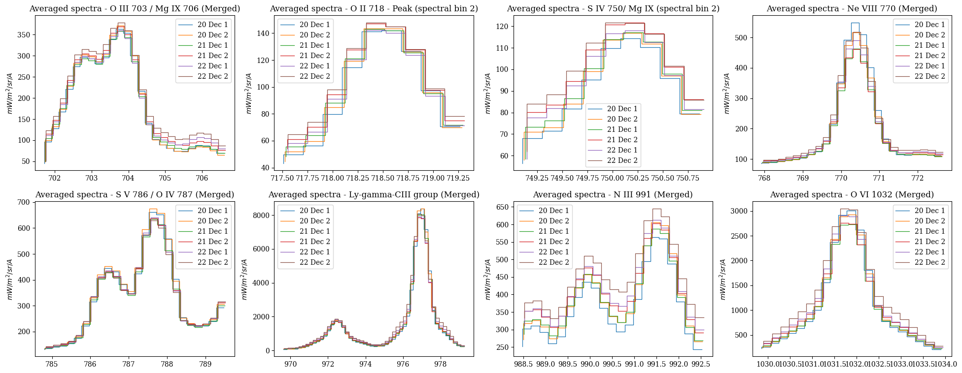
Figure 8: Average spectra over the footpoint of AR 13169, computed over an area of 15x30 pixels. Each color represents a different observation time.

Each raster contains 8 windows: O III 703 / Mg IX 706, O II 718 - Peak, S IV 750 / Mg IX, Ne VIII 770, S V 786 / O IV 787, Ly-gamma-CIII group, N III 991 and O VI 1032. Those windows and their average spectra for each raster are plotted in Figure 8, and the contribution functions for some lines of interest are plotted in Figure 1.

Two Active Regions (ARs) were caught in the dataset from December 2022: NOAA 13171 and NOAA 13169. Both of them are registered as $\beta$-class ARs. Their characteristics are summarized in Table 1.

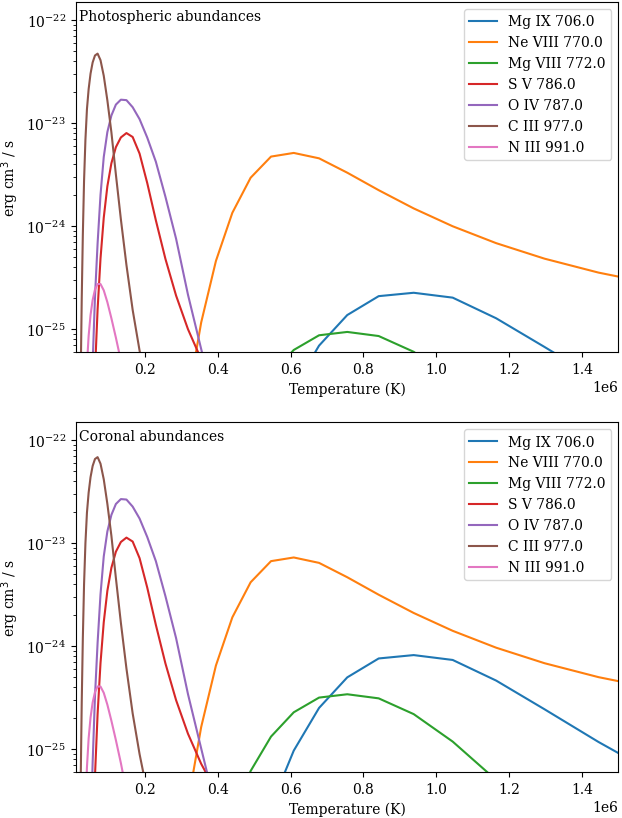
Figure 1: Contribution functions for the SPICE lines of interest. A density of $n_{e}=2\times 10^{9}$ cm^-3 has been assumed. Top panel: photospheric abundances, bottom panel: coronal abundances.

	NOAA 13169	NOAA 13171
Hale class	$\beta$ / $\beta$-$\gamma$	$\beta$
Start date	2022/12/17	2022/12/19
End date	2022/12/30	2022/12/31
Max. sunspot area	490	250 (millionths)
Max. nbr of spots	30	12
Associated flares	3 M-class	6 C-class

Table 1: Technical description of observed ARs.

NOAA 13169 stays the longest in SPICE’s FOV, and therefore has been targeted for the rest of the analysis. The AR was first observed on December 17, 2022, already presenting a bipolarity in its sunspot structure. During its observation by SPICE, the AR is within its late, slow emerging phase (see Figure 2). Its magnetic configuration is complex enough that opposite polarity spots cannot be clearly distinguished. Figure 3 shows the evolution of the AR seen in the SDO/AIA (Lemen et al., 2012) 171 Å  band, and the corresponding magnetograms from HMI (Scherrer et al., 2012). The latter are plotted within the range of $\pm$ 200 G. The leading positive polarity sunspot group stays consistent through the observations, bordered by a negative, more dispersed field on its west side.

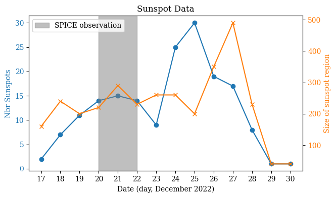
Figure 2: Evolution of AR 13169 in terms of sunspot number (blue curve) and sunspot area (orange curve). Data is the courtesy of https://www.spaceweatherlive.com. During this period, 3 M-class flares abd 61 C-class flares have been recorded. The time of the observations stuided here is highlighted in gray.

Two main outflows are seen in the EUV FOV. On December 22, a full loop can be observed within SPICE’s raster (see Figure 3, bottom panel). This loop seems to be newly formed, linking the very strong positive magnetic field area to the negative area. Further confirmation of high magnetic activity is provided by the flares associated with the AR (on December 20, one M1.1-class flare at 13:59 UT and eight C-class were associated to AR13169).

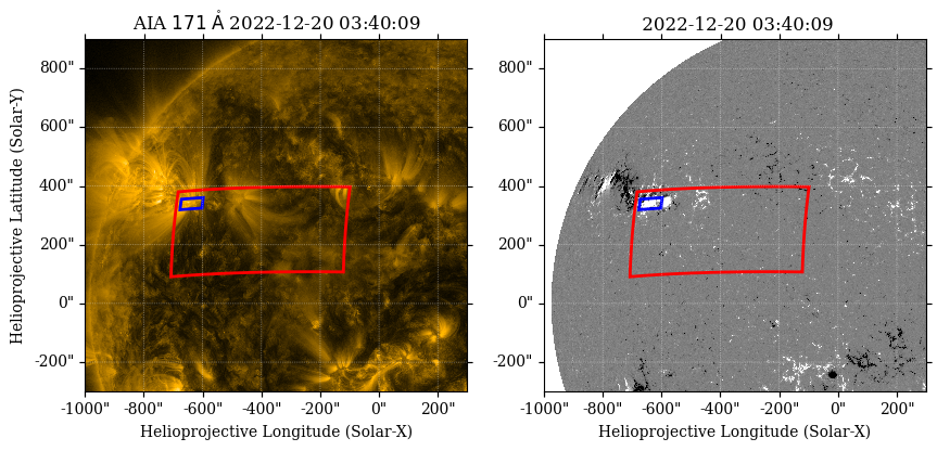
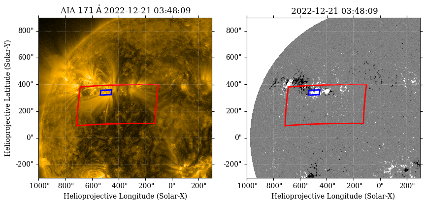
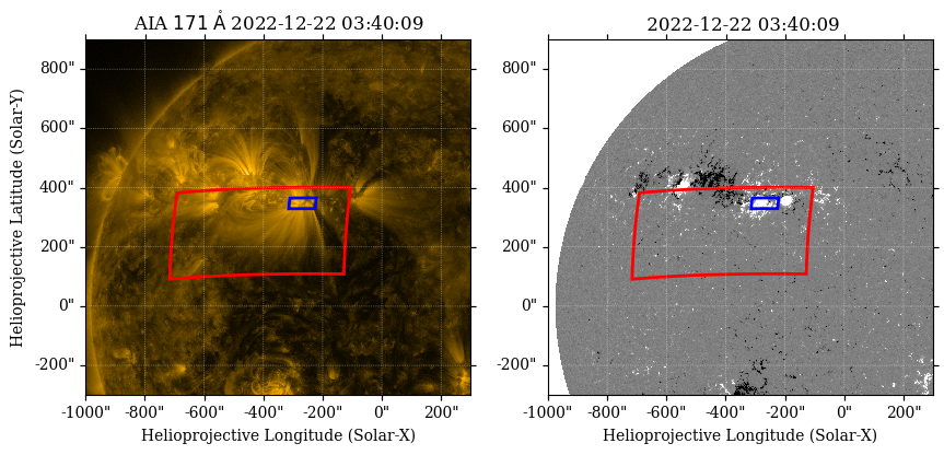
Figure 3: Evolution of AR 13169 (depicted as the blue rectangle) in SPICE’s approximate FOV (red rectangle) from 2022 December 20 to 2022 December 22, seen in SDO/AIA 171 Å  and corresponding SDO/HMI magnetograms. On the magnetograms, white/black areas represent positive/negative polarity. Blue areas are of significant positive magnitude.

Spectral lines	logT (K)	FIP (eV)	Transition	Sub-windows ($\AA$)
O i 988.6	4.2	13.6	2s2 2p4 3P2 - 2s2 2p3 2D0	987.4 – 989.1
H i 972.5	4.5	13.6	1s2 2S1/2 - 5p 2P1/2	969.0 – 974.5
O ii 718 (mult.)	4.7	13.6	2s2 2p3 2D5/2 - 2s 2p4 2D5/2	716.3 – 720.9
C iii 977	4.8	11.3	2s2 1S0 - 2s 2p 1P1	974.5 – 980.3
N iii 989	4.8	14.5	2s2 2p 2P1/2 - 2s 2p2   2D3/2	989.1 – 990.6
N iii 991	4.8	14.5	2s2 2p 2P3/2 - 2s 2p2   2D3/2	990.6 – 993.4
O iii 702.8	4.9	13.6	2s2 2p2 3P1 - 2s 2p3 3P0	700.3 – 703.1
O iii 703.8	4.9	13.6	2s2 2p2 3P2 - 2s 2p3 3P1	703.1 – 704.8
S iv 750	5.0	10.4	3s2 3p 2P3/2 - 3s 3p2 2P3/2	749.8 – 752.5
S v 786	5.2	10.4	3s2 1S0 - 3s 3p 1P1	784.2 – 787.0
O iv 787	5.2	13.6	2s2 2p 2P1/2 - 2s 2p2 2D3/2	787.0 – 789.8
O vi 1032	5.4	13.6	1s2 2s 2S1/2 - 1s2 2p 2P3/2	1029.1 – 1034.9
Ne viii 770	5.8	21.6	1s2 2s 2S1/2 - 1s2 2p 2P3/2	767.2 – 771.5
Mg viii 772	5.9	7.6	2s2 2p  2P3/2 - 2s2p2 4P5/2	771.5 – 775.2
Mg ix 749	6.0	7.6	2s2 1S0 - 2s 2p 3P1	747.8 – 749.8
Mg ix 706	6.0	7.6	2s2 1S0 - 2s 2p 3P1	704.85 – 708.1

Table 2: Lines extracted from the SPROUT dataset, and the wavelength window used to determine the Gaussian parameters for the fitting.

3 Methods

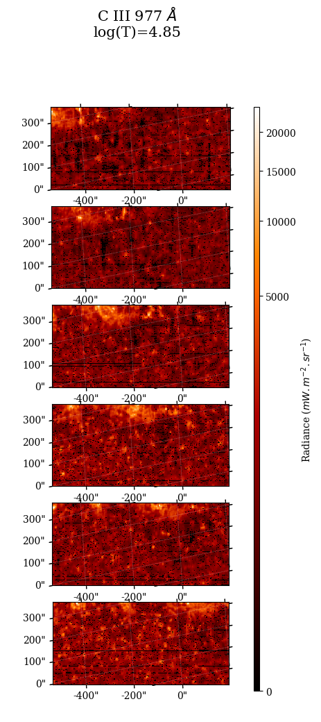
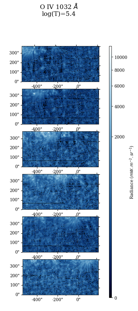
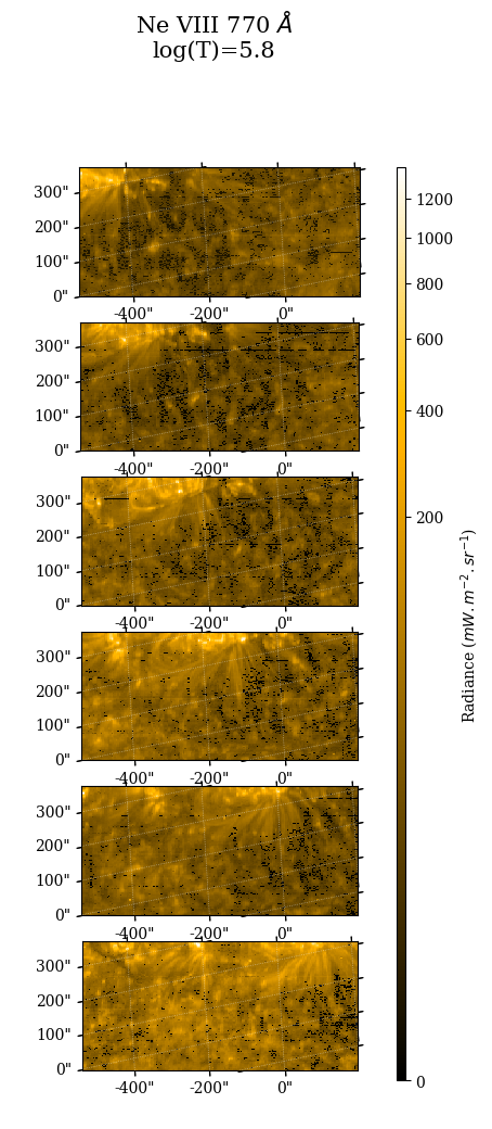
Figure 9: Radiance maps seen in the C III 977 Å, O VI 1032 Å and Ne VIII 770 Å lines from December 20-22 2022. The field of view is focused on AR 13169 (upper parts of the panels).

Figure 9 shows C III 977 Å, O VI 1032 Å and Ne VIII 770 Å  radiance maps. All radiance maps were obtained by fitting the spectral lines with a Gaussian model, using sub-windows and multiple Gaussian curves (up to three) if several emission peaks were present in a single window (see Table 2). O II 718 - Peak and O VI 1032 are the only windows containing a single emission peak. S IV 750 / Mg IX, Ne VIII 770 and Ly-gamma-CIII contained two distinct emission peaks, and O III 703 / Mg IX 706, S V 786 / O IV 787 and N III 991 presented three.

Line	Radiances QS	Radiances AR
O iii 702.8	24.8 $\pm$ 20.4	77.6 $\pm$ 9.7
O iii 703.8	24.1 $\pm$ 19.7	84.2 $\pm$ 6.3
Mg ix 706	3.3 $\pm$ 19.7	33.7 $\pm$ 5.4
Mg ix 749	4.3 $\pm$ 23.4	15.8 $\pm$ 4.7
S iv 750	4.6 $\pm$ 23.6	26.2 $\pm$ 4.9
Ne viii 770	34.4 $\pm$ 26.3	302.1 $\pm$ 48.5
Mg viii 772	4.3 $\pm$ 25.3	32.7 $\pm$ 8.1
S v 786	28.5 $\pm$ 28.7	132.3 $\pm$ 10.5
O iv 787	60.5 $\pm$ 29.3	18.5 $\pm$ 14.5
C iii 977	677.0 $\pm$ 43.0	3386.5 $\pm$ 254.2
N iii 989.8	26.8 $\pm$ 12.3	114.2 $\pm$ 15.8
N iii 991.5	39.1 $\pm$ 12.3	290.1 $\pm$ 26.5
O vi 1032	202.2 $\pm$ 18.0	1611.5 $\pm$ 173.2

Table 3: Radiance values from December 20-22 2022 for a Quiet Sun region (QS) and an Active Region (AR 13169). As can be seen in the Table, the QS values for the lines Mg IX 749, S IV 750 and Mg VIII 772 can not be trusted due to extremely high deviation.

To compute the relative FIP bias, we used four different line ratios, covering different ranges of temperatures, and therefore regions in the solar atmosphere. Two of them involve the O IV line: S V 786 Å (low-FIP proxy, 10.4 eV, $\log(T)=5.2$) and O IV 787 Å (high-FIP, 13.6 eV, $\log(T)=5.2$) and C III 997 Å  (low-FIP proxy, 11.3eV, $\log(T)=4.8$) and the same O IV line. The other two ratios are Mg VIII 772 Å  (low-FIP, 7.6 eV, $\log(T)=5.9$) and Ne VIII 770 Å  (very-high FIP, 21.6 eV, $\log(T)=5.8$) and the S V 786 Å line paired with N III 991 Å (high-FIP, 14.5 eV, $\log(T)=4.8$).

Even though sulfur and carbon are considered as intermediate-FIP, we still use them in our diagnostics for two reasons: 1) to investigate the behavior of those ambiguous elements, knowing that they exhibit different behaviors based on magnetic configuration 2) C/O has a similar electron configuration as Si/S, which is a common ratio used for FIP bias computation in spectroscopy, particularly by the EIS spectrometer on board the Hinode mission (Culhane et al., 2007a; Baker et al., 2015; Mihailescu et al., 2022).

To account for contribution function differences as well as temperature and density effects, we included a differential emission measure (DEM) factor in our FIP bias computation. We do later derive DEMs from SPICE. Also DEM variance are too large for a reference DEM to be acceptable. Actual computed DEMs need to be used instead. The FIP bias is thus numerically computed as

$$FIP_{bias}=\frac{I_{LF}}{I_{HF}}\left(\frac{Ab^{P}_{LF}}{Ab^{P}_{HF}}\frac{C_{LF}\cdot\text{DEM}}{C_{HF}\cdot\text{DEM}}\right)^{-1}$$ (2)

Where $LF$ and $HF$ denote respectively the low-FIP and high-FIP elements.

Determining the Differential Emission Measure (DEM) from observed radiances in multiple spectroscopic lines is a challenging task due to the limitations of integral inversion methods, such as data insufficiency and the ill-conditioned nature of the problem, particularly in the density dimension(Craig & Brown, 1976; Judge et al., 1997). Most DEM determination techniques require prior density measurements, and inversion methods often struggle to accurately resolve the general shape and finer details of the DEM, especially for multithermal plasmas, where solutions are biased to specific temperature ranges (Testa et al., 2012; Guennou et al., 2012). However, we use here Plowman & Caspi (2020)’s method, and this enables a realistic estimation of the DEM directly from the same data used to compute the radiance, allowing for a consistent determination of the FIP bias as well. We checked that variations in the density chosen (here, $n_{e}=2\times 10^{9}$) do not affect significantly the contribution function. Once the DEM estimates are computed, they are plugged in Equation 2.

In Figure 4 are presented the results of the Emission Measure (EM) and DEM for the right footpoint of AR 13196 on December 21, 2022 at 03:34 UT. The EM loci shows a unique intersection at logT = 5.8, further confirmed by the DEM showing that most of the contribution comes from material around logT = 5.8.

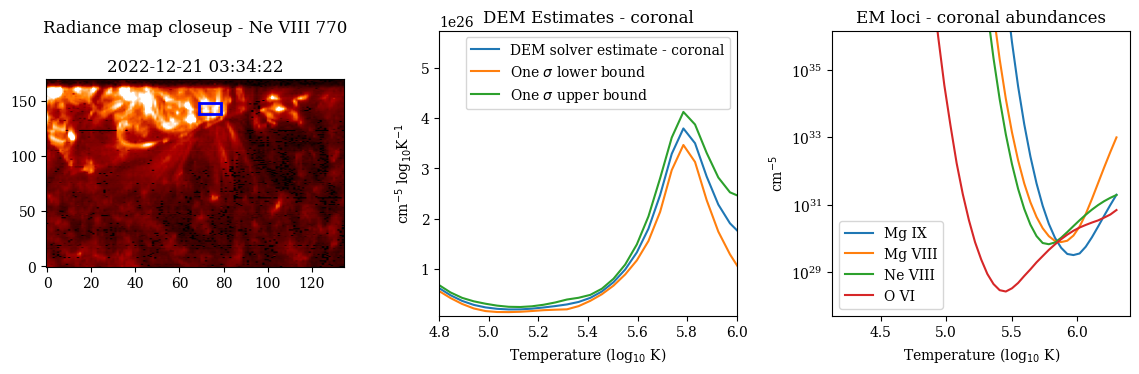
Figure 4: EM loci, DEM estimation and corresponding zone on the Ne VIII 770 Å map. Both the EM loci and DEM estimation indicate a rather isothermal emission around logT=5.8 for the region observed.

4 Modeling

Following the model developed in Laming (2017); Laming et al. (2019), FIP fractionation is estimated for the active region observed. This model describes the observed fractionation of elemental abundances in the solar atmosphere, assuming a quasistatic framework for long-lived structures like coronal loops, active regions, and solar wind outflow regions. Within these static scenarios, fractionation in closed loops is thought to take place in the upper chromosphere.

The ponderomotive force acts primarily on the low-FIP elements, which have a significantly higher ionization fraction than high-FIP elements (see top middle and right panels in Figure 6). This force preferentially lifts them toward the top of the transition region. Upon reaching this region, two key changes occur: the temperature rises enough to fully ionize both low and high FIP elements, eliminating the distinction between ions and neutrals, and the density gradient becomes smaller, causing the ponderomotive force to vanish. As a result, the fractionation process ceases at the transition region’s upper boundary, locking in the established fractionation pattern. Other mechanisms then are thought to transport the fractionated plasma into the corona.

The parameters taken consists of a loop 80,000 km long and with a 100 G magnetic field. Waves have angular frequencies of 0.332 and 0.665 (fundamental and first harmonic), with amplitudes chosen to give FIP fractionations around 4 with respect to oxygen. Figure 5 shows the results of the modeling for the loop parameters. It is clear that the ponderomotive acceleration peaks at the footpoints of the loop, meaning that plasma fractionation very likely occurs at the same height along the loop.

Figure 5: Top panel: magnetic field and velocity perturbations (variation of the components of the Elsässer variables), real (in black) and imaginary parts (in red). The middle panel depicts the left and right going wave energy fluxes, and their differences (the latter are flat since there are no sinks or sources of waves involved in the calculation). Bottom panel: ponderomotive acceleration along the loop.

The modeled FIP fractionation values are represented in Figure 6. The key feature is on the right panel, where low-FIP elements start to behave significantly differently with respect to the high-FIP elements in the upper chromosphere. While low-FIP elements become more abundant, the high-FIP elements are depleted. The intermediate element sulfur, which supposedly behaves as a high-FIP element in closed magnetic structures (see Baker et al. (2024) and references therein), stays at a constant ionization rate. However, it is interesting to note that in the ponderomotive force model, S/O qualitatively looks a low-FIP element, being enhanced rather than depleted at a chromospheric altitude of 220 km, even though by not very much (see Figure 6).

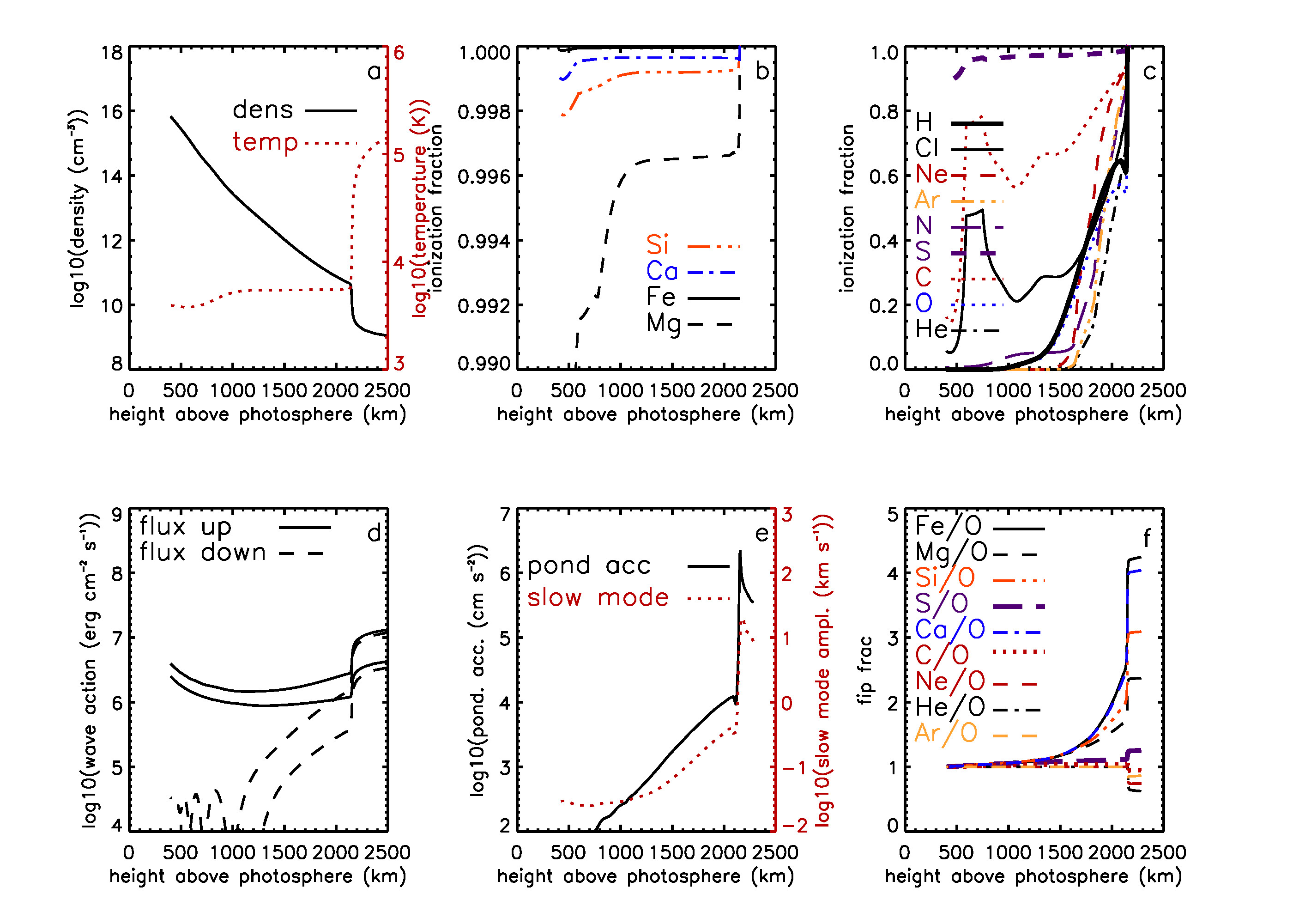
Figure 6: Top panels, from left to right: chromospheric density and temperature structure, low FIP ionization fractions and high FIP ionization fractions. Bottom panels, from left to right: wave energy fluxes, ponderomotive acceleration and slow mode wave amplitudes, and fractionations with height in the chromosphere. While the Fe/O ratio increases, the S/O does not. This behavior is typical of resonant waves on closed loops.

5 Results

Previous studies have demonstrated that the fractionation process takes place in the upper chromosphere where Alfvén waves are refracted, causing the FIP effect due to the ponderomotive force (Laming, 2017, and references therein). Fractionation seems to depend on the magnetic field geometry. In open field regions, the dependence of fractionation on the plasma upflow velocity through the chromosphere is modeled for both shear (or planar) and torsional Alfvén waves originating from the photosphere. In closed field regions, the fractionation produced by Alfvén waves originates from both photospheric and coronal regions (Laming, 2015). These differences in behavior have a significant impact on the behavior of intermediate-FIP elements (Kuroda & Laming, 2020). This characteristic is clearly illustrated in Figure 7: the ratios involving the intermediate-FIP element sulfur do not evolve. This behavior supports the hypothesis suggesting that sulfur behaves as a high-FIP element in closed magnetic structures (Laming et al., 2019).

The ratios corresponding to different solar atmospheric layers have been computed using the methods described in Section 2.

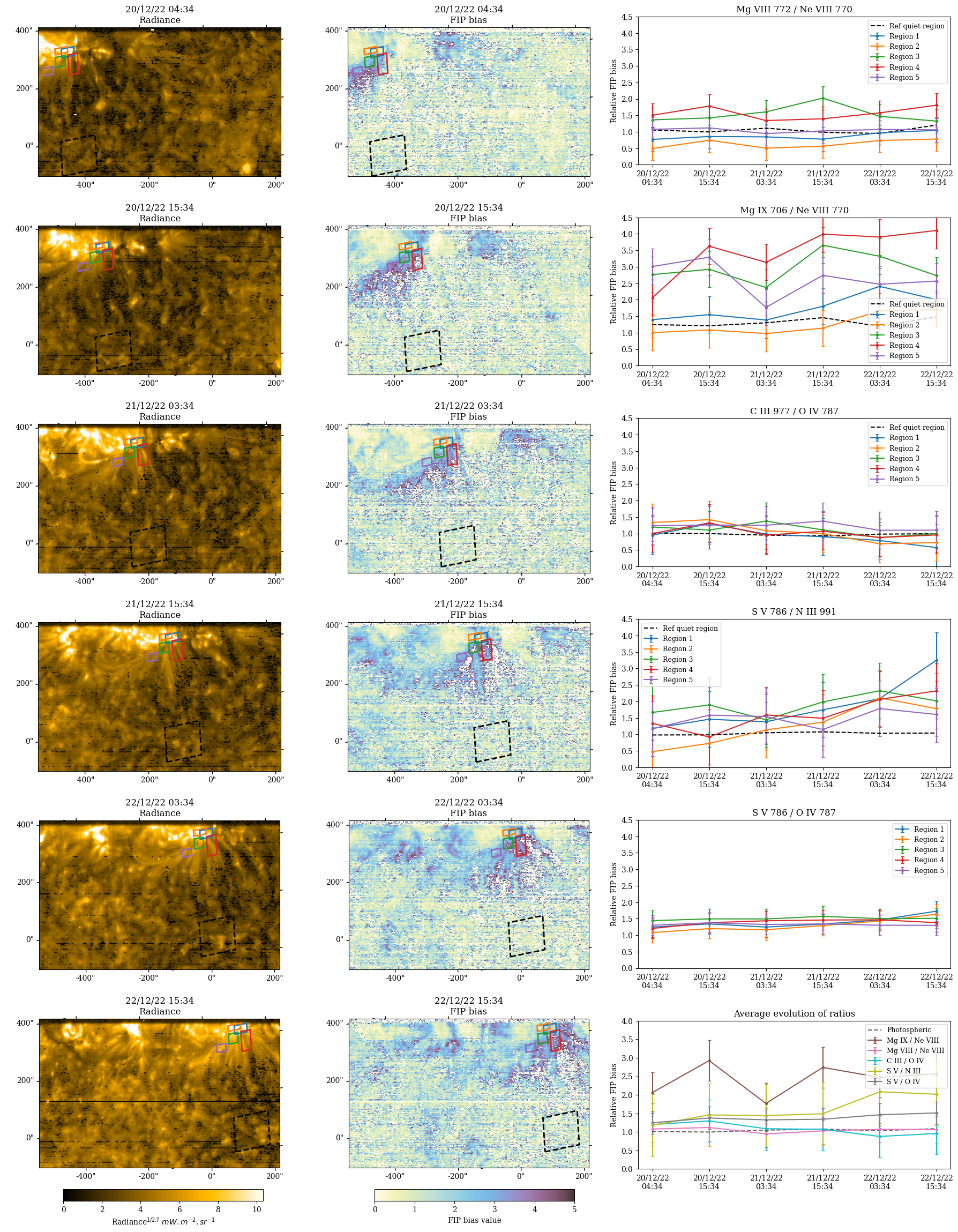
Figure 7: Evolution of AR 13169 in SPICE’s field of view. Left column: Radiance maps seen in the Ne VIII 770 line (logT=5.8). Middle panel: FIP bias maps seen in the Mg IX / Ne VIII ratio. Right column: Evolution of the FIP bias values, tracking different zones. The black dotted line represents the photospheric / quiet Sun reference.

Kuroda & Laming (2020) did not observe an increase of C/O alongside S/O, as predicted by their models. Studies on solar energetic particles (SEPs) typically estimate the C/O abundance ratio to be around 0.7, indicating a fractionation of about 1.3 based on the photospheric abundance. However, it is still not yet understood why the measured C/O ratio on open and closed fields remains close to the expected ratio from closed-field fractionation models (values ranging from 1.1 to 1.5 (Laming, 2015)).

The right footpoint of AR 13169 has been tracked by using several macropixels. Results of the tracking are shown in Figure 7. The ratio involving sulfur seem to stay relatively constant around 1.3 for the first two days, but then shows a slight increase to reach values around 2. Accounting for the uncertainties in the DEM and the difference in temperature of the two lines, this could be consistent with the fact that S behaves as a high-FIP in closed-field regions and as a low-FIP element in open-field regions (Laming et al., 2019). The final abundance ratios (December 22, 2022) inferred from SPICE data match decently well with the model presented in Figure 5, smililarly to Mihailescu et al. (2023)’s work. In this model, Mg/Ne = 2.98, S/N=1.74, and C/O = 0.96. However, the start of the observation series have a different behavior. C III 977/O IV 787 and S V 750/N III 991 could be affected by absorption by the H I continuum. The spectra early in the study could be affected by absorption by intervening H I, while those later on are not, presumably because enough of the loop has emerged to sufficiently higher altitudes. This would affect lines shortward of 918 Angstroms, so the C III/O IV ratio would be increased and S V/N III would be decreased. The only ratios that might not be affected would be Mg VIII/Ne VIII and S V/O IV. The lines are so close in wavelength that the H I absorption would affect them both the same, having no impact on the FIP bias computation.

Both Mg/Ne ratios show a very high variability depending on the region targeted. The Mg IX/Ne VIII ratio does show a global increase while the ratio involving Mg VIII looks more quiet. The very slow rate of increasing FIP bias matches the fact that the AR 13169 is in a slow emerging phase, so that the waves are stuck and resonate within the loop. It seems like regions 3 and 4, located just at the edge of the AR core, exhibit more coronal-like behavior, while closer to the core, the values seem to be photospheric or even inverse-FIP like. This structure-dependant factor could be linked to what Warren et al. (2016) identified, which is that intense heating events show close to photospheric composition, while more stable structures like coronal ”fans” are consistent with the usual coronal composition. Similar behavior has also been observed in Doschek et al. (2015) in the Ar/Ca ratio, which has an electron configuration similar to Mg/Ne.

The C/O ratio shows a very slight, steady decrease over time, starting around 1.2 / 1.5 and reaching less than 1 after 3 days. It is very interesting to note that the S/O ratio shows a very slight increase, matching almost perfectly the values in the ponderomotive model and therefore exhibiting more low-FIP like behavior.

This could suggest that: 1) the carbon has already been fractionated because of its intermediate-FIP behavior 2) we observe different heights in the solar atmosphere at the same time. The magnesium is then observed to have a coronal abundance later in time, because of the time necessary to transport the fractionated plasma upper up in the solar atmosphere. Kuroda & Laming (2020) suggested that the enhancement of intermediate-FIP elements was taking place in the lower chromosphere, where H is not ionized. This phenomenon is even more pronounced in the areas where non-resonant waves are present, which is a characteristic of open-field regions.

From this set of SPICE observations, we cannot clearly state that the FIP bias is a quantity generally dependent of time. Combining the observations with models, it appears that the FIP bias is dependent on height in the chromosphere. However, once the plasma reaches the transition region, where it becomes fully ionized, no further FIP fractionation occurs. In this set of observations, the AR is emerging slowly. The waves in the magnetic field are stuck in the structure and resonate like in an optics resonant cavity, giving the FIP bias time to develop and increase. Looking at the evolution of the magnetic structure over the set of dates studied, we observe numerous flux cancellation events around the right footpoint of AR 13169. These phenomena could lead to the emergence of new photospheric flux, leading to the lower values oberved in Figure 7.

We seek to bring elements of an answer to the following questions:

• Is the fractionation process driven by waves?

• Does the time delay induced by resonant Alfven waves until they undergo total internal refraction and then escape matches with the delay observed between different line ratios?

Even though there are still discrepancies between models and observations for changes in abundances, both converge more and more in recent years. These first results of SPICE SPROUTS’ rasters suggest that fractionation happens at a chromospheric level and that the fractionated plasma is brought at the top of the transition region after a time delay of about 24 hours. Understanding the differences between FIP bias diagnostics and the mechanisms of the fractionation of S will be crucial for linking in situ plasma observations to their solar surface origin, as S is a frequent observation in both remote sensing and in situ FIP bias diagnostics.

6 Discussion and Conclusions

Investigating the FIP effect and its evolution regarding different variables is essential to understand the fractionation mechanisms of photospheric plasma. From SPICE’s observations and our diagnostics, we can conclude that waves are highly likely to cause fractionation. The fact that the Mg/Ne increases is what is expected if the waves causing the fractionation are resonant with the coronal loop, which almost certainly means that they are generated in the coronal part of the loop subject to the boundary conditions at the loop footpoints, analog to an optical resonating cavity. The slowly decrease of C/O could be an indicator of transport mechanisms at work, but in this work we assume that there is sufficient turbulence or collisions to mix the plasma, and that the only agent of fractionation is the ponderomotive force. This assumption put first, the behavior of C/O could be explained by the H I continuum absorption.

Plasma mixing, flux emergence and cancellation seem to be an important factor in the observed values of FIP bias. Depending on the structure of the region observed, and potentially adjacent coronal holes, plasma mixing and emergence of new photospheric flux is highly likely.

Observing different behaviors for different magnesium lines could be explained by the difference in temperature and therefore contribution functions, which are a crucial part of estimating DEMs and computing FIP bias. Further observations and analysis would be useful to assess which ratio is the most reliable, knowing that Mg IX usually has a better signal-to-noise ratio, but Mg VIII has a closer temperature and wavelength to Ne VIII.

In their study, Widing & Feldman (2001) postulate that coronal loops emerge with photospheric abundances, and only become coronal-abundant when at least a part of the loop reaches the corona. With this postulate and recent results, including the observations made in this work, the FIP effect observed in this scenario is likely caused by a cascade of events starting from the corona.

It is rather hazardous and beyond the scope of this paper to go further and to try to match the rate of temperature increase with the wave energy times the damping rate. Indeed, there is no consensus of the wave damping mechanisms and their rate. This is why we estimated it with the wave energy given by that required for the FIP effect. As mentioned before, the model is quasistatic, whereas the AR observed has some dramatic events at the time of observations like M-class flares, introducing smaller scale evolution.

These SPICE SPROUTS observations provide needed insight into the evolution of the FIP bias, looking at lower heights to investigate the chromospheric origin of plasma fractionation. The large number of spectral lines recorded and the recurrent recordings enable us to follow the fractionation of elements from the chromosphere to the corona and in time.

Coupling SPICE’s observations with high-resolution EUV imaging from Solar Orbiter’s EUI (Rochus et al., 2022), unfortunately unavailable at the time of these observations, could provide insightful material to discriminate regimes of FIP fractionation, i.e. if the plasma observed fractionates low or high in the chromosphere and its associated mechanisns. The SWA/HIS instrument (Owen, C. J. et al., 2020), part of SolO’s in-situ suite, could also provide connectivity and further confirmation of solar wind streams coming out of the regions studied.

The current study focuses on a specific subset of the SPROUTS observations to establish a robust methodological framework for these novel observations. Future studies will build upon this foundation and incorporate data from other solar observatories. In future work, we plan to extend our analysis to include a broader range of data sources pertaining to this AR and the slow solar wind possibly emanating from its eastern boundary.

Further investigation into the evolution of this AR can be achieved by utilizing observations from other missions. The Extreme-Ultraviolet Imaging Spectrometer (Culhane et al., 2007b) on board the Hinode (Kosugi et al., 2007) mission observed the AR on the days following the SPICE observations. Measurements of Doppler velocities, densities, and other abundance diagnostics could provide additional context as well as insights into the AR’s continued evolution. By utilizing the Polarimetric and Helioseismic Imager (PHI) (Solanki, S. K. et al., 2020) and advanced modelling, we could extrapolate the coronal magnetic field. This would allow us to better visualize the magnetic structure of the AR itself and understand its interrelationship with the structures observed in the EUV images, as the Sun’s magnetic field drives the dynamics and structure of the solar corona. Magnetic field extrapolations also help determine where the plasma reaching Solar Orbiter originates, as shown in Figure B3 in the appendix. Combining these model predictions with the analysis of in-situ data would give us a clearer idea if the plasma from this AR would eventually reach the spacecraft through reconnection at the boundary with the coronal hole to its south. Notably, SWA-HIS (Owen, C. J. et al., 2020), which measures heavy ion abundances in the solar wind, recorded data on the days following these spectroscopic observations and the data is now available. In addition to these efforts, other data sets of SPROUTS observations will allow us to further explore temporal changes in a wider variety of solar structures.

Appendix A Spectra and Radiance maps

Appendix B Connectivity

In Figure 10 are presented two Sun - Spacecraft connectivity maps corresponding to the afternoon observations (around 15:00 UT) on the 20 (top panel) and 21 (bottom panel) December 2022. The solar wind measured from the estimated footpoint (depicted as a red dot) exhibits a slower speed, suggesting a source of slow solar wind. The source is linked to the eastern boundary of AR 13169, corresponding to the high FIP bias observed with SPICE (see Figure 7).

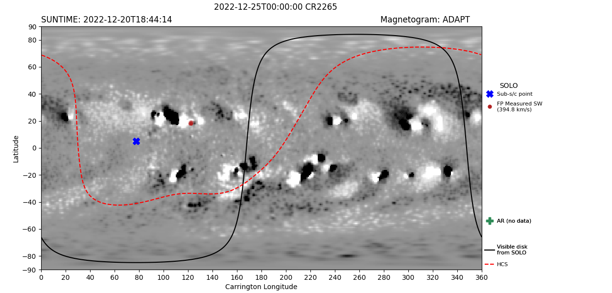
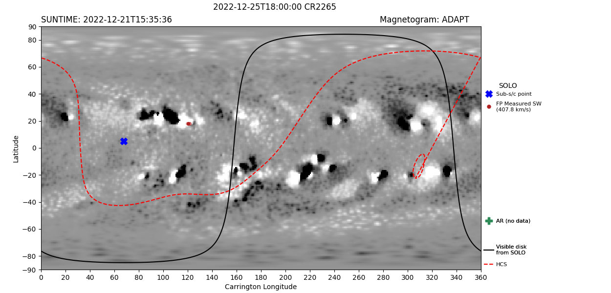
Figure 10: ADAPT connectivity maps obtained from the MADAWG Connectivity Tool (MCT) found at http://connect-tool.irap.omp.eu/. The top panel shows the connectivity at Sun/Spacecraft dates of 2022 December 20 / 2022 December 25. Bottom panel shows 18 hours (spacecraft time) later. Slow solar wind connectivities are depicted by the red circles, and the estimated sub-spacecraft point is shown by the blue cross.

References

- Baker et al. (2013) Baker, D., Brooks, D. H., Démoulin, P., et al. 2013, The Astrophysical Journal, 778, 69, doi: 10.1088/0004-637X/778/1/69
- Baker et al. (2015) —. 2015, ApJ, 802, 104, doi: 10.1088/0004-637X/802/2/104
- Baker et al. (2018) Baker, D., Brooks, D. H., van Driel-Gesztelyi, L., et al. 2018, The Astrophysical Journal, 856, 71
- Baker et al. (2024) Baker, D., van Driel-Gesztelyi, L., James, A. W., et al. 2024, ApJ, 970, 39, doi: 10.3847/1538-4357/ad4a6e
- Brooks et al. (2022) Brooks, D. H., Janvier, M., Baker, D., et al. 2022, The Astrophysical Journal, 940, 66, doi: 10.3847/1538-4357/ac9b0b
- Craig & Brown (1976) Craig, I. J. D., & Brown, J. C. 1976, A&A, 49, 239
- Culhane et al. (2007a) Culhane, J. L., Harra, L. K., James, A. M., et al. 2007a, Sol. Phys., 243, 19, doi: 10.1007/s01007-007-0293-1
- Culhane et al. (2007b) —. 2007b, Sol. Phys., 243, 19, doi: 10.1007/s01007-007-0293-1
- Doschek et al. (2015) Doschek, G., Warren, H., & Feldman, U. 2015, The Astrophysical Journal Letters, 808, L7
- Guennou et al. (2012) Guennou, C., Auchère, F., Soubrié, E., et al. 2012, ApJS, 203, 25, doi: 10.1088/0067-0049/203/2/25
- Judge et al. (1997) Judge, P. G., Hubeny, V., & Brown, J. C. 1997, ApJ, 475, 275, doi: 10.1086/303511
- Ko et al. (2016) Ko, Y.-K., Young, P. R., Muglach, K., Warren, H. P., & Ugarte-Urra, I. 2016, The Astrophysical Journal, 826, 126
- Kosugi et al. (2007) Kosugi, T., Matsuzaki, K., Sakao, T., et al. 2007, Sol. Phys., 243, 3, doi: 10.1007/s11207-007-9014-6
- Kuroda & Laming (2020) Kuroda, N., & Laming, J. M. 2020, ApJ, 895, 36, doi: 10.3847/1538-4357/ab8870
- Laming (2015) Laming, J. M. 2015, Living Reviews in Solar Physics, 12, 2, doi: 10.1007/lrsp-2015-2
- Laming (2017) —. 2017, ApJ, 844, 153, doi: 10.3847/1538-4357/aa7cf1
- Laming (2021) —. 2021, ApJ, 909, 17, doi: 10.3847/1538-4357/abd9c3
- Laming et al. (2019) Laming, J. M., Vourlidas, A., Korendyke, C., et al. 2019, ApJ, 879, 124, doi: 10.3847/1538-4357/ab23f1
- Lanzafame et al. (2002) Lanzafame, A. C., Brooks, D. H., Lang, J., et al. 2002, A&A, 384, 242, doi: 10.1051/0004-6361:20011662
- Lemen et al. (2012) Lemen, J. R., Title, A. M., Akin, D. J., et al. 2012, Sol. Phys., 275, 17, doi: 10.1007/s11207-011-9776-8
- Meyer (1985) Meyer, J. P. 1985, ApJS, 57, 173, doi: 10.1086/191001
- Meyer (1991) Meyer, J.-P. 1991, Advances in Space Research, 11, 269, doi: https://doi.org/10.1016/0273-1177(91)90120-9
- Mihailescu et al. (2022) Mihailescu, T., Baker, D., Green, L. M., et al. 2022, The Astrophysical Journal, 933, 245, doi: 10.3847/1538-4357/ac6e40
- Mihailescu et al. (2023) Mihailescu, T., Brooks, D. H., Laming, J. M., et al. 2023, ApJ, 959, 72, doi: 10.3847/1538-4357/ad05bf
- Müller et al. (2020) Müller, D., St. Cyr, O. C., Zouganelis, I., et al. 2020, A&A, 642, A1, doi: 10.1051/0004-6361/202038467
- Owen, C. J. et al. (2020) Owen, C. J., Bruno, R., Livi, S., et al. 2020, A&A, 642, doi: 10.1051/0004-6361/201937259
- Plowman & Caspi (2020) Plowman, J., & Caspi, A. 2020, The Astrophysical Journal, 905, 17, doi: 10.3847/1538-4357/abc260
- Rochus et al. (2022) Rochus, P., Auchère, F., Berghmans, D., et al. 2022, A&A, 665, C1, doi: 10.1051/0004-6361/201936663e
- Réville et al. (2021) Réville, V., Rouillard, A. P., Velli, M., et al. 2021, Frontiers in Astronomy and Space Sciences, 8, doi: 10.3389/fspas.2021.619463
- Scherrer et al. (2012) Scherrer, P. H., Schou, J., Bush, R. I., et al. 2012, Sol. Phys., 275, 207, doi: 10.1007/s11207-011-9834-2
- Sheeley (1995) Sheeley, N. R., J. 1995, ApJ, 440, 884, doi: 10.1086/175326
- Solanki, S. K. et al. (2020) Solanki, S. K., del Toro Iniesta, J. C., Woch, J., et al. 2020, A&A, 642, A11, doi: 10.1051/0004-6361/201935325
- Testa et al. (2012) Testa, P., De Pontieu, B., Martínez-Sykora, J., Hansteen, V., & Carlsson, M. 2012, ApJ, 758, 54, doi: 10.1088/0004-637X/758/1/54
- To et al. (2021) To, A. S., Long, D. M., Baker, D., et al. 2021, The Astrophysical Journal, 911, 86
- Varesano et al. (2024) Varesano, T., Hassler, D. M., Zambrana Prado, N., et al. 2024, A&A, 685, A146, doi: 10.1051/0004-6361/202347637
- Warren et al. (2016) Warren, H. P., Brooks, D. H., Doschek, G. A., & Feldman, U. 2016, The Astrophysical Journal, 824, 56
- Widing (1997) Widing, K. G. 1997, The Astrophysical Journal, 480, 400, doi: 10.1086/303947
- Widing & Feldman (2001) Widing, K. G., & Feldman, U. 2001, The Astrophysical Journal, 555, 426, doi: 10.1086/321482
- Young & Mason (1997) Young, P. R., & Mason, H. E. 1997, Sol. Phys., 175, 523, doi: /10.1023/A:1004936106427