Determination of Hubble constant from Megamaser Cosmology Project using Profile Likelihood

Abstract

The Megamaser Cosmology Project inferred a value for the Hubble constant given by $H_{0}=73.9\pm 3.0$ km/sec/Mpc. This value was obtained using Bayesian inference by marginalizing over six nuisance parameters, corresponding to the velocities of the megamaser galaxy systems. We obtain an independent estimate of the Hubble constant with the same data using frequentist inference. For this purpose, we use profile likelihood to dispense with the aforementioned nuisance parameters. The frequentist estimate of the Hubble constant is given by $H_{0}=73.5^{+3.0}_{-2.9}$ km/sec/Mpc and agrees with the Bayesian estimate to within $0.2\sigma$, and both approaches also produce consistent confidence/credible intervals. Therefore, this analysis provides a proof of principle application of profile likelihood in dealing with nuisance parameters in Cosmology, which is complementary to Bayesian analysis.

1 Introduction

One of the most vexing problems in the current concordance $\Lambda$CDM model is the so-called Hubble tension, which refers to a $5\sigma$ discrepancy between measurement of the Hubble constant ($H_{0}$) based on Cosmic Microwave background based measurements and those based on low-redshift probes such as Cepheid calibrated Type Ia Supernovae (Abdalla et al., 2022; Verde et al., 2019; Bethapudi and Desai, 2017; Shah et al., 2021; Freedman, 2021; Di Valentino et al., 2021; Verde et al., 2024). This discrepancy has been considered very seriously by the cosmology community and could be a harbinger of new Physics (Kamionkowski and Riess, 2023), although see  Vagnozzi (2023) for a contrarian viewpoint.

One important data analysis aspect in all recent estimates of $H_{0}$ is that the final value of $H_{0}$ has been obtained using Bayesian inference after marginalizing over other cosmological or astrophysical nuisance parameters. The marginalization is usually done using Markov Chain Monte Carlo methods (Sharma, 2017). In fact, almost all cosmological analyses in the last two decades have been done using Bayesian inference (Trotta, 2008) with very few exceptions (See  Ade et al. 2014; Nielsen et al. 2016 for some counter-examples). In particle physics, on the other hand, parameter inference has always been done using Frequentist techniques, where the nuisance parameters get dispensed with using the concept of Profile Likelihood (Cowan, 2013).

Recently, it has been demonstrated within the Cosmology community, that the process of marginalization, inherent in Bayesian analysis, could be affected by prior volume effects and can bias the final results (Gómez-Valent, 2022). Therefore, after the advent of the Hubble tension conundrum, there has been a resurgence in the application of profile likelihood techniques to parameter inference in Cosmology (Herold et al., 2022; Herold and Ferreira, 2023; Campeti and Komatsu, 2022; Colgáin et al., 2024; Karwal et al., 2024; Sah et al., 2024) (and references therein). In particular, Herold et al. (2022) has shown that some of the null results or upper limits on early dark energy obtained with Bayesian inference using MCMC were affected by volume effects. However, when profile likelihood was used to deal with the nuisance parameters, one finds $2\sigma$ evidence for early dark energy. Therefore, it behooves us to test wherever possible if the Bayesian estimates of $H_{0}$ agree with the frequentist estimates.

In this manuscript, we obtain an independent estimate of $H_{0}$ using data from the Megamaser Cosmology Project (Pesce et al., 2020b) (P20, hereafter), using frequentist inference. This work is a follow-up to our recent papers on applications of profile likelihood to search for Lorentz Invariance Violation using Gamma-ray burst spectral lags (Desai and Ganguly, 2024; Ramakrishnan and Desai, 2025). For the megamaser analysis, we first independently reproduce some of the results in P20 with Bayesian inference using MCMC and then compare these results with Frequentist inference. This manuscript is structured as follows. In Sect. 2, we provide a brief summary of the procedure used in P20 to estimate $H_{0}$. We, then, independently reproduce these results with Bayesian inference in Sect. 3 and Frequentist inference in Sect. 4. We then conclude in Sect. 5.

2 Analysis of megamaser data in P20

It has been known for a while that water megmasers in accretion disks around supermassive black holes provide very good geometric probes of distances (Herrnstein et al., 1999). The Megamaser Cosmology Project has been designed for this purpose, to find such megamaser systems and use them to measure $H_{0}$ (Braatz et al., 2008; Reid et al., 2009, 2019; Pesce et al., 2020a). Such a measurement of $H_{0}$ is independent of distance ladder and is therefore complementary to Cepheid based and CMB-based techniques.

In 2020, P20 reported a measurement of $H_{0}$ using six megamaser systems with their estimated value given by $H_{0}=73.9\pm 3.0$ km/sec/Mpc. We now provide a brief summary of the analysis done in the aforementioned work.

P20 obtained precise angular diameter distance ($D_{A}$) and velocity estimates to six megamaser systems. The expression for $D_{A}$ for a galaxy at a redshift ($z_{i}$) for a flat $\Lambda$CDM cosmology is given by:

$$D_{A}=\frac{c}{H_{0}\left(1+z_{i}\right)}\int_{0}^{z_{i}}\frac{\text{d}z}{\sqrt{\Omega_{m}\left(1+z\right)^{3}+\left(1-\Omega_{m}\right)}}$$ (1)

where $\Omega_{m}$ is the cosmological matter density, for which P20 used the value of 0.315. The expected recession velocity ($v_{i}$) is then related to redshift by

$$v_{i}=cz_{i}$$ (2)

To estimate $H_{0}$, P20 constructed a likelihood given by $-0.5\chi^{2}$, where $\chi^{2}$ is given by the following expression:

$$\chi^{2}=\sum_{i}\left[\frac{\left(v_{i}-\hat{v}_{i}\right)^{2}}{\sigma_{v,i}^{2}+\sigma_{\text{pec}}^{2}}+\frac{(D_{A}-\hat{D}_{A})^{2}}{\sigma_{D,a}^{2}}\right],$$ (3)

where $\hat{v}_{i}$ is the measured galaxy velocity and $\sigma_{v,i}$ is the corresponding uncertainty; $\sigma_{\text{pec}}$ is the uncertainty in the peculiar velocity assumed to be 250 km/sec; $\hat{D}_{A}$ is the distance measured from disk modeling while $\sigma_{D,a}$ denotes its uncertainty. In Eq. 3, the true velocity ($v_{i}$) is treated as a nuisance parameter, and the true redshift is related to the true velocity from Eq. 2. The regression problem therefore involves seven free parameters, namely $H_{0}$ and six true velocities, corresponding to each of the six megamaser galaxy systems. P20 used Bayesian inference for this analysis. They used uniform priors for all the free parameters and used dynesty (Speagle, 2020) Nested sampler to sample the posterior constructed using the likelihood defined earlier. The marginalized value for $H_{0}$ obtained using this method is given by $H_{0}=73.9\pm 3.0$ km/sec/Mpc. Subsequently, different approaches were used in correcting the peculiar velocities, which do not modify $H_{0}$ by more than $1\sigma$. More details on this can be found in P20.

3 Bayesian estimate of $H_{0}$

Before proceeding to frequentist analysis, we independently reproduce the results in P20 using Bayesian regression, following the discussion in the previous section. For our regression analysis, we define the unknown parameter vector by {$H_{0}$,$v_{1}$,$v_{2}$,$v_{3}$,$v_{4}$,$v_{5}$,$v_{6}$}, where {$v_{1}$, $v_{2}$,..,$v_{6}$} denote the unknown true velocities of the six megamaser galaxy systems, which are treated as nuisance parameters. We use uniform priors for each of the true velocities given by $v_{i}\in\mathcal{U}(500,20000)$ in units of km/sec and $H_{0}\in\mathcal{U}(50,200)$ in units of km/sec/Mpc. We sample the likelihood using emcee sampler (Foreman-Mackey et al., 2013) and show the marginalized posteriors for each of the seven free parameters using the getdist package (Lewis, 2019). The marginalized credible intervals for all the seven free parameters are shown in Fig. 1. The marginalized $1\sigma$ estimate for $H_{0}$ is given by $H_{0}=73.9\pm 3.0$ km/sec/Mpc, which agrees with the value reported in P20 of $H_{0}=73.9\pm 3.0$ km/sec/Mpc.

Figure 1: Marginalized 68%, 95%, and 99% credible intervals for all the seven free parameters used in analysis of megamaser data. The marginalized $1\sigma$ central estimate of $H_{0}$ is given by $73.9\pm 3.0$ km/sec/Mpc. {$v1,v2,...,v6$} correspond to the true velocities of UGC 3789, NGC 6264, NGC 6323, NGC 5765b, CGCG 074-064, and NGC 4258, respectively.

4 Frequentist estimate of $H_{0}$

We now carry out a frequentist analysis of the megamaser data in order to estimate $H_{0}$, where we use profile likelihood to deal with the six nuisance parameters. More details on the basic principles behind profile likelihood can be found in  Herold et al. (2024) or our recent works (Desai and Ganguly, 2024; Ramakrishnan and Desai, 2025), and references therein.

We first construct a grid for $H_{0}$ uniformly spaced between 60-80 km/sec/Mpc. For each fixed value of $H_{0}$ on this grid, we minimize $\chi^{2}$ in Eq. 3 over the remaining six free parameters to obtain $\chi^{2}(H_{0})$. This minimization for each fixed value of $H_{0}$ was done using the scipy.optimize.minimize library in Python. We tried six different minimization algorithms available in this function, namely Nelder-Mead Simplex method, Powell, CG, BFGS, Newton-CG and L-BFGS-B algorithm . We also tested minimization using the iminuit library, which has previously been shown to be more robust than scipy (Campeti and Komatsu, 2022). However, for our minimization function, all the aforementioned algorithms return the same minimum value of $\chi^{2}$ at each value of $H_{0}$. We then calculate the minimum $\chi^{2}$ among the different values of $\chi^{2}(H_{0})$, and plot $\Delta\chi^{2}$ as a function of $H_{0}$ where

$$\Delta\chi^{2}=\chi^{2}(H_{0})-\chi^{2}_{min}$$ (4)

This plot of $\Delta\chi^{2}$ as a function of $H_{0}$ can be found in Fig. 2. In case the best-fit value is close to the physical boundary, one uses the Feldman-Cousins prescription (Feldman and Cousins, 1998). However, since the minimum value obtained is far from the physical boundary, we use the Neyman prescription to get the central estimates for $H_{0}$ (Neyman, 1937) To obtain the 68.3% ($1\sigma$) confidence level estimates of $H_{0}$, we find the $X$-intercept corresponding to $\Delta\chi^{2}=1.0$ (Press et al., 1992). The $1\sigma$ central estimate of $H_{0}$ is then given by $H_{0}=73.5^{+3.0}_{-2.9}$ km/sec/Mpc. We can see that the best-fit values agree with the Bayesian estimate within $0.2\sigma$ and they also produce consistent confidence intervals.

Therefore, we have conducted a proof-of-principle application of profile likelihood by applying it to the problem of estimating $H_{0}$ using data from the Megamaser Cosmology Project. In this case, the results from both the frequentist and Bayesian estimates give statistically indistinguishable results, whereas previously, these methods have led to discordant results for some other regression problems in Astrophysics and Cosmology (Herold et al., 2022; Desai and Ganguly, 2024; Ramakrishnan and Desai, 2025).

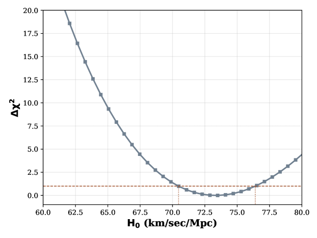
Figure 2: $\Delta\chi^{2}$ (cf. Eq. 4) as a function of $H_{0}$ after using profile likelihood to deal with the six nuisance parameters. The dashed horizontal line corresponds to $\Delta\chi^{2}=1$ and the dotted line shows the corresponding $X$-intercept used to obtain our frequentist estimate of $H_{0}$. The $1\sigma$ estimate of $H_{0}$ is given by $73.5^{+3.0}_{-2.9}$ km/sec/Mpc.

5 Conclusions

In this manuscript, we obtain an independent estimate of $H_{0}$ with data from the Megamaser Cosmology Project using frequentist inference. The main difference between the two methods is the treatment of nuisance parameters. In Bayesian inference, the nuisance parameters are dispensed with using marginalization, whereas in frequentist inference, profile likelihood is used for the same. This estimate of $H_{0}$ was first done using Bayesian inference in P20, which obtained a value of $73.9\pm 3.0$ km/sec/Mpc. This estimate of $H_{0}$ involved marginalization over six nuisance parameters, corresponding to the velocities of the six megamaser galaxy systems used for the analysis. We first reproduced the result using Bayesian inference and independently obtained the value of $H_{0}=73.9\pm 3.0$ km/sec/Mpc (cf Fig. 1), which agrees with the P20 estimate. We then redid the analysis using frequentist inference and obtained the value of $H_{0}=73.5^{+3.0}_{-2.9}$ km/sec/Mpc (cf. Fig. 2). Therefore, the frequentist estimate of $H_{0}$ agrees with the result from Bayesian analysis within $0.2\sigma$. Furthermore both approaches yield consistent confidence/credible intervals, thus implying that the results are statistically indistinguishable. Therefore, this estimate of $H_{0}$ provides another proof of principle application of profile likelihood in dealing with nuisance parameters.

References

- Abdalla et al. (2022) Abdalla, E., et al., 2022. Cosmology intertwined: A review of the particle physics, astrophysics, and cosmology associated with the cosmological tensions and anomalies. JHEAp 34, 49–211. doi:10.1016/j.jheap.2022.04.002, arXiv:2203.06142.
- Ade et al. (2014) Ade, P.A.R., et al. (Planck), 2014. Planck intermediate results. XVI. Profile likelihoods for cosmological parameters. Astron. Astrophys. 566, A54. doi:10.1051/0004-6361/201323003, arXiv:1311.1657.
- Bethapudi and Desai (2017) Bethapudi, S., Desai, S., 2017. Median statistics estimates of Hubble and Newton’s constants. European Physical Journal Plus 132, 78. doi:10.1140/epjp/i2017-11390-3, arXiv:1701.01789.
- Braatz et al. (2008) Braatz, J.A., Reid, M.J., Greenhill, L.J., Condon, J.J., Lo, K.Y., Henkel, C., Gugliucci, N.E., Hao, L., 2008. Investigating Dark Energy with Observations of H2O Megamasers, in: Bridle, A.H., Condon, J.J., Hunt, G.C. (Eds.), Frontiers of Astrophysics: A Celebration of NRAO’s 50th Anniversary, p. 103.
- Campeti and Komatsu (2022) Campeti, P., Komatsu, E., 2022. New Constraint on the Tensor-to-scalar Ratio from the Planck and BICEP/Keck Array Data Using the Profile Likelihood. Astrophys. J. 941, 110. doi:10.3847/1538-4357/ac9ea3, arXiv:2205.05617.
- Colgáin et al. (2024) Colgáin, E.Ó., Pourojaghi, S., Sheikh-Jabbari, M.M., 2024. Implications of DES 5YR SNe Dataset for CDM. arXiv e-prints , arXiv:2406.06389doi:10.48550/arXiv.2406.06389, arXiv:2406.06389.
- Cowan (2013) Cowan, G., 2013. Statistics for Searches at the LHC. arXiv e-prints , arXiv:1307.2487doi:10.48550/arXiv.1307.2487, arXiv:1307.2487.
- Desai and Ganguly (2024) Desai, S., Ganguly, S., 2024. Constraint on Lorentz Invariance Violation for spectral lag transition in GRB 160625B using profile likelihood. arXiv e-prints , arXiv:2411.09248doi:10.48550/arXiv.2411.09248, arXiv:2411.09248.
- Di Valentino et al. (2021) Di Valentino, E., Mena, O., Pan, S., Visinelli, L., Yang, W., Melchiorri, A., Mota, D.F., Riess, A.G., Silk, J., 2021. In the realm of the Hubble tension-a review of solutions. Classical and Quantum Gravity 38, 153001. doi:10.1088/1361-6382/ac086d, arXiv:2103.01183.
- Feldman and Cousins (1998) Feldman, G.J., Cousins, R.D., 1998. Unified approach to the classical statistical analysis of small signals. Phys. Rev. D 57, 3873–3889. doi:10.1103/PhysRevD.57.3873, arXiv:physics/9711021.
- Foreman-Mackey et al. (2013) Foreman-Mackey, D., Hogg, D.W., Lang, D., Goodman, J., 2013. emcee: The MCMC Hammer. PASP 125, 306. doi:10.1086/670067, arXiv:1202.3665.
- Freedman (2021) Freedman, W.L., 2021. Measurements of the Hubble Constant: Tensions in Perspective. Astrophys. J. 919, 16. doi:10.3847/1538-4357/ac0e95, arXiv:2106.15656.
- Gómez-Valent (2022) Gómez-Valent, A., 2022. Fast test to assess the impact of marginalization in Monte Carlo analyses and its application to cosmology. Phys. Rev. D 106, 063506. doi:10.1103/PhysRevD.106.063506, arXiv:2203.16285.
- Herold and Ferreira (2023) Herold, L., Ferreira, E.G.M., 2023. Resolving the Hubble tension with early dark energy. Phys. Rev. D 108, 043513. doi:10.1103/PhysRevD.108.043513, arXiv:2210.16296.
- Herold et al. (2024) Herold, L., Ferreira, E.G.M., Heinrich, L., 2024. Profile Likelihoods in Cosmology: When, Why and How illustrated with CDM, Massive Neutrinos and Dark Energy. arXiv e-prints , arXiv:2408.07700doi:10.48550/arXiv.2408.07700, arXiv:2408.07700.
- Herold et al. (2022) Herold, L., Ferreira, E.G.M., Komatsu, E., 2022. New Constraint on Early Dark Energy from Planck and BOSS Data Using the Profile Likelihood. Astrophys. J. Lett. 929, L16. doi:10.3847/2041-8213/ac63a3, arXiv:2112.12140.
- Herrnstein et al. (1999) Herrnstein, J.R., Moran, J.M., Greenhill, L.J., Diamond, P.J., Inoue, M., Nakai, N., Miyoshi, M., Henkel, C., Riess, A., 1999. A geometric distance to the galaxy NGC4258 from orbital motions in a nuclear gas disk. Nature 400, 539–541. doi:10.1038/22972, arXiv:astro-ph/9907013.
- Kamionkowski and Riess (2023) Kamionkowski, M., Riess, A.G., 2023. The Hubble Tension and Early Dark Energy. Annual Review of Nuclear and Particle Science 73, 153–180. doi:10.1146/annurev-nucl-111422-024107, arXiv:2211.04492.
- Karwal et al. (2024) Karwal, T., Patel, Y., Bartlett, A., Poulin, V., Smith, T.L., Pfeffer, D.N., 2024. Procoli: Profiles of cosmological likelihoods. arXiv e-prints , arXiv:2401.14225doi:10.48550/arXiv.2401.14225, arXiv:2401.14225.
- Lewis (2019) Lewis, A., 2019. GetDist: a Python package for analysing Monte Carlo samples. arXiv e-prints , arXiv:1910.13970doi:10.48550/arXiv.1910.13970, arXiv:1910.13970.
- Neyman (1937) Neyman, J., 1937. Outline of a theory of statistical estimation based on the classical theory of probability. Philosophical Transactions of the Royal Society of London. Series A, Mathematical and Physical Sciences 236, 333–380.
- Nielsen et al. (2016) Nielsen, J.T., Guffanti, A., Sarkar, S., 2016. Marginal evidence for cosmic acceleration from Type Ia supernovae. Scientific Reports 6, 35596. doi:10.1038/srep35596, arXiv:1506.01354.
- Pesce et al. (2020a) Pesce, D.W., Braatz, J.A., Reid, M.J., Condon, J.J., Gao, F., Henkel, C., Kuo, C.Y., Lo, K.Y., Zhao, W., 2020a. The Megamaser Cosmology Project. XI. A Geometric Distance to CGCG 074-064. Astrophys. J. 890, 118. doi:10.3847/1538-4357/ab6bcd, arXiv:2001.04581.
- Pesce et al. (2020b) Pesce, D.W., Braatz, J.A., Reid, M.J., Riess, A.G., Scolnic, D., Condon, J.J., Gao, F., Henkel, C., Impellizzeri, C.M.V., Kuo, C.Y., Lo, K.Y., 2020b. The Megamaser Cosmology Project. XIII. Combined Hubble Constant Constraints. Astrophys. J. Lett. 891, L1. doi:10.3847/2041-8213/ab75f0, arXiv:2001.09213.
- Press et al. (1992) Press, W.H., Teukolsky, S.A., Vetterling, W.T., Flannery, B.P., 1992. Numerical recipes in FORTRAN. The art of scientific computing.
- Ramakrishnan and Desai (2025) Ramakrishnan, V., Desai, S., 2025. Constraints on Lorentz Invariance Violation from Gamma-ray Burst rest-frame spectral lags using Profile Likelihood. arXiv e-prints , arXiv:2502.00805doi:10.48550/arXiv.2502.00805, arXiv:2502.00805.
- Reid et al. (2009) Reid, M.J., Braatz, J.A., Condon, J.J., Greenhill, L.J., Henkel, C., Lo, K.Y., 2009. The Megamaser Cosmology Project. I. Very Long Baseline Interferometric Observations of UGC 3789. Astrophys. J. 695, 287–291. doi:10.1088/0004-637X/695/1/287, arXiv:0811.4345.
- Reid et al. (2019) Reid, M.J., Pesce, D.W., Riess, A.G., 2019. An Improved Distance to NGC 4258 and Its Implications for the Hubble Constant. Astrophys. J. Lett. 886, L27. doi:10.3847/2041-8213/ab552d, arXiv:1908.05625.
- Sah et al. (2024) Sah, A., Rameez, M., Sarkar, S., Tsagas, C., 2024. Anisotropy in Pantheon+ supernovae. arXiv e-prints , arXiv:2411.10838doi:10.48550/arXiv.2411.10838, arXiv:2411.10838.
- Shah et al. (2021) Shah, P., Lemos, P., Lahav, O., 2021. A buyer’s guide to the Hubble constant. Astronomy and Astrophysics Review 29, 9. doi:10.1007/s00159-021-00137-4, arXiv:2109.01161.
- Sharma (2017) Sharma, S., 2017. Markov Chain Monte Carlo Methods for Bayesian Data Analysis in Astronomy. Ann. Rev. Astron. Astrophys. 55, 213–259. doi:10.1146/annurev-astro-082214-122339, arXiv:1706.01629.
- Speagle (2020) Speagle, J.S., 2020. DYNESTY: a dynamic nested sampling package for estimating Bayesian posteriors and evidences. MNRAS 493, 3132–3158. doi:10.1093/mnras/staa278, arXiv:1904.02180.
- Trotta (2008) Trotta, R., 2008. Bayes in the sky: Bayesian inference and model selection in cosmology. Contemporary Physics 49, 71–104. doi:10.1080/00107510802066753, arXiv:0803.4089.
- Vagnozzi (2023) Vagnozzi, S., 2023. Seven Hints That Early-Time New Physics Alone Is Not Sufficient to Solve the Hubble Tension. Universe 9, 393. doi:10.3390/universe9090393, arXiv:2308.16628.
- Verde et al. (2024) Verde, L., Schöneberg, N., Gil-Marín, H., 2024. A Tale of Many H 0. Ann. Rev. Astron. Astrophys. 62, 287–331. doi:10.1146/annurev-astro-052622-033813, arXiv:2311.13305.
- Verde et al. (2019) Verde, L., Treu, T., Riess, A.G., 2019. Tensions between the early and late Universe. Nature Astronomy 3, 891–895. doi:10.1038/s41550-019-0902-0, arXiv:1907.10625.