Blank Space: Adaptive Causal Coding for Streaming Communications Over Multi-Hop Networks

Abstract

In this work, we introduce Blank Space AC-RLNC (BS), a novel Adaptive and Causal Network Coding (AC-RLNC) solution designed to mitigate the triplet trade-off between throughput-delay-efficiency in multi-hop networks. BS leverages the network’s physical limitations considering the bottleneck from each node to the destination. In particular, BS introduces a light-computational re-encoding algorithm, called Network AC-RLNC (NET), implemented independently at intermediate nodes. NET adaptively adjusts the Forward Error Correction (FEC) rates and schedules idle periods. It incorporates two distinct suspension mechanisms: 1) Blank Space Period, accounting for the forward-channels bottleneck, and 2) No-New No-FEC approach, based on data availability. The experimental results achieve significant improvements in resource efficiency, demonstrating a $20\%$ reduction in channel usage compared to baseline RLNC solutions. Notably, these efficiency gains are achieved while maintaining competitive throughput and delay performance, ensuring improved resource utilization does not compromise network performance.

I Introduction

The exponential growth in streaming applications, demanding high data rates and low latency, has pushed wireless connectivity beyond traditional point-to-point schemes toward multi-hop networks, where intermediate nodes cooperate and share the common medium. However, as these networks evolve, ensuring efficient use of power consumption and spectrum utilization while maintaining high goodput and low delay is essential. The difficulty increases when the wireless channel is noisy, dynamic, and unknown. These conditions are all common to both modern and future terrestrial and non-terrestrial networks, such as Unmanned Aerial Vehicles (UAV) networks [1], Mobile Ad-Hoc Networks (MANETs) [2] and Wireless Sensor Networks (WSN) [3].

Network Coding (NC) [4], particularly Random Linear Network Coding (RLNC) [5, 6], has demonstrated the ability to achieve the min-cut max-flow capacity in multi-hop networks, though it struggles to meet ultra-low delay requirements in streaming communications due to its large blocklength regime. Alternative approaches like rateless [7, 8] and stemming codes for point-to-point communications [9, 10, 11, 12, 13, 14] have been proposed to address delay concerns. However, these solutions remain sensitive to channel variations as they lack adaptation mechanisms [15, 16, 17, 18, 19, 20]. Adaptive and Causal RLNC (AC-RLNC) recently proposed in [21, 22], employs an adaptive-size sliding window on coded packets based on channel state estimation. AC-RLNC utilizes two key mechanisms: an a-priori Forward Error Correction (FEC) mechanism that compensates for expected erasures, and an a-posteriori feedback-based FEC mechanism that handles lost packets [21, 23, 24, 25]. This approach, leveraging per-packet acknowledgments, makes AC-RLNC suitable for Ultra-Reliable Low Latency Communications (URLLC) [26].

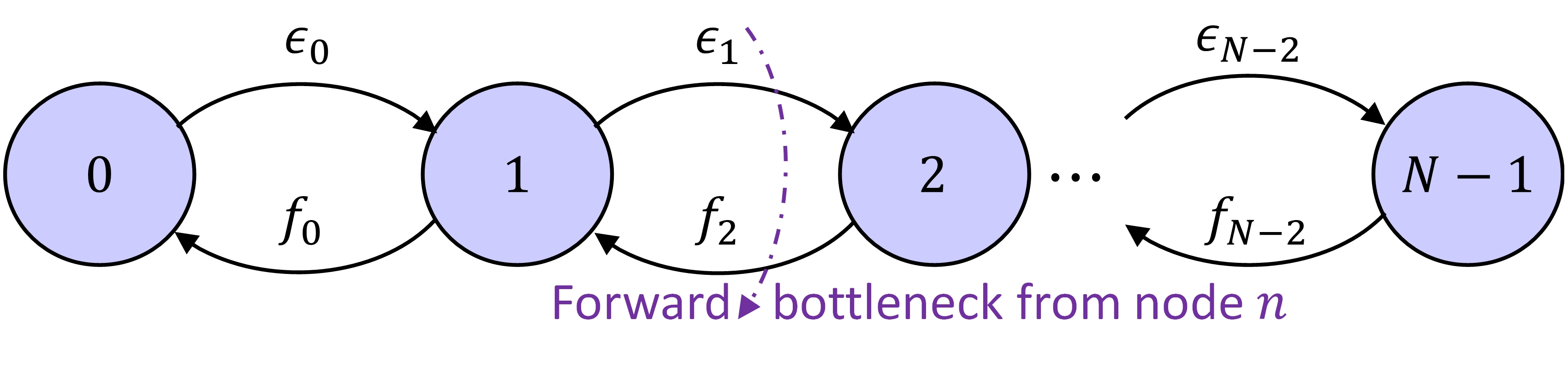
Figure 1: Multi-hop communication system with $N$ nodes. The dashed line represents the forward bottleneck from node $n$ to the destination estimated for the proposed Network AC-RLNC in BS. Here, for example, for node $n=1$ the estimated forward bottleneck, $\epsilon_{1}$, is larger from $\{\epsilon_{2},\ldots,\epsilon_{N-2}\}$, but not necessarily from $\epsilon_{0}$.

In this work, we provide a coding-based solution that mitigates the trade-off between throughput-delay-efficiency in multi-hop networks. Optimizing this trade-off remains an open question, and to the best of our knowledge, this is the first work addressing this problem using RLNC. We propose Blank Space AC-RLNC (BS), a novel adaptive and causal solution that generalizes AC-RLNC to achieve the desired triplet trade-off in multi-hop networks. In BS, intermediate nodes may employ Network AC-RLNC (NET), a light-computational re-encoding algorithm. NET enables nodes to adaptively adjust their re-transmission rates based on channel conditions (similarly to the source in AC-RLNC) and schedule idle periods to prevent ineffective transmissions. The nodes manage their sliding coding windows based on decoding assessment rather than actual packet decoding, eliminating the decoding computational overhead. NET introduces two transmission suspension mechanisms: 1) Blank Space Period, which considers the forward channels bottleneck - see Fig. 1, and 2) No-New No-FEC approach, which stems from the BS algorithm structure of independently operating nodes, based on the current buffer state and content. These two mechanisms effectively reduce the channel usage rate and increase the goodput, while maintaining high delivery rates and low in-order delivery delay.

Our experimental results demonstrate that a substantial improvements in resource efficiency while reducing channel usage. For example, for a setting with a network bottleneck of $40\%$ erasure rate, the channel usage drops by $20\%$ for the end-to-end network, and up to $40\%$ for individual nodes, compared to baseline RLNC implementation. This usage rate further decreases as the global bottleneck erasure rate increases. Notably, the increase in efficiency is achieved while maintaining competitive performance in the rate-delay trade-off for URLLC, ensuring that improved resource utilization does not come at the cost of degraded network performance.

II System Model and Preliminaries

This section presents our system model and key preliminaries. We begin by introducing the communication model in Subsection II-A, followed by the problem formulation in Subsection II-B. We then review the relevant background in adaptive and causal network coding in Subsection II-C.

II-A System Model

Consider a multi-hop real-time slotted communication system with $N$ nodes, ranging from node $0$ (source) to node $N-1$ (destination). Each pair of adjacent nodes $(n,n+1)$ communicates over a directional noisy forward channel, denoted as $e_{n}$, for $n\in\{0,1,...,N-2\}$. A noiseless feedback channel, $f_{n}$, used to send acknowledgments, is available in the reverse direction. This multi-hop network is illustrated in Fig 1. At each time slot $t<T$, node $n$ can transmit a packet over its forward channel $e_{n}$, where $T>0$ is the time horizon. These forward channels are modeled as Binary Erasure Channels (BECs) - For each channel $e_{n}$, packet erasures occur with independently probability $\epsilon_{n}$ at any time slot $t\leq T$. The corresponding channel rates in the asymptotic regime where $t\rightarrow\infty$ are $r_{n}=1-\epsilon_{n}$, the capacity of BEC channel [27].

For any node $n$, we define its forward-channels bottleneck ${BN}_{n}$, as the channel index with the highest erasure rate along the remaining forward path, that is,

$$\textstyle{BN}_{n}=\underset{{n\leq i\leq N-2}}{\text{argmax}}\left\{\epsilon_{i}\right\}.$$ (1)

The global bottleneck in the multi-hop network, denoted by ${\rm BN}$, is therefore ${BN}_{0}$.

We do not assume prior knowledge of the forward channel’s erasure rate. However, each node does have access to delayed local feedback and may use it to estimate the channel’s statistics. Specifically, each pair of nodes has its own round trip time denoted by $\rm RTT_{n}$. For simplicity, we assume symmetric propagation delays of $\frac{\rm RTT_{n}}{2}$ in both forward and feedback channels. The global propagation delay from the source to the destination is therefore, $\frac{\rm RTT}{2}$ where $\rm RTT=\sum_{n=0}^{N-2}\rm RTT_{n}$. Upon receiving a packet from node $n$, node $n+1$ transmits either an acknowledgment (ACK) or a negative-acknowledgment (NACK) message back to node $n$ over the noiseless feedback channel, $f_{n}$. For a packet transmitted at time $t$, we denote its feedback message from node $n+1$ as $F_{t}^{n+1}$, where $F_{t}^{n+1}=1$ indicates an ACK and $F_{t}^{n+1}=0$ indicates a NACK. For a batch of $M$ received feedback messages, the estimated erasure rate of forward channel $e_{n}$, is given by

$$\textstyle\hat{\epsilon}_{n}=1-\frac{1}{M}\sum_{i=0}^{M}{F_{i}^{n}}.$$ (2)

Each node has a buffer to store incoming packets, which may arrive one per time slot (including the source). The source operates as encoder, which encodes available information packets and transmits a coded packet to the next node. Each intermediate node operates as a re-encoder, capable of encoding incoming coded packets into new coded packets. We distinguish between information packets, $p_{i}$ (the $i$th packet arrived at the source) and packets (any coded packet transmitted over any of the forward channels). The packets are denoted by $c_{t}^{n}$, representing a coded packet transmitted from node $n$ at time $t$. For any information packet $p_{i}$, we define $T_{1}(p_{i})$ as the arrival time at the source node and $T_{d}(p_{i})$ as its decoding time at the destination. $d(t)$ represents the cumulative number of information packets decoded at the destination by time $t$.

Any transmitting node $n$ begins operation after an initial delay of $\sum_{i=0}^{n}\frac{\mathrm{RTT_{i}}}{2}$, since this is the first time it may receive a packet. During operation, a node may pause transmission at any time slot, in which case no packet is sent. The number of these idle slots for node $n$ is denoted by $O_{n}$ (excluding the initial delay period).

II-B Problem Formulation

Our goal herein is threefold: 1) maximize data delivery, 2) minimize in-order delivery delay, and 3) minimize channel usage. Hence, we will use the following performance metrics.

1) Normalized Goodput, $\eta$: The total amount of information delivered to the destination in units of bits per second, divided by the total amount of bits transmitted by the source in this period. Since we consider a slotted transmission with a fixed number of $T$ time slots where one packet may be transmitted at each slot and a constant packet size, the normalized goodput can be calculated as,

$$\textstyle\eta\triangleq\frac{d(T)}{T-O_{0}-\frac{\rm RTT}{2}},$$ (3)

recalling $d(T)$ is the total number of information packets decoded by the end of the network operation.

2) Delivery Rate, $R_{\rm{del}}$: The total amount of information delivered to the destination in units of bits per second for some $T^{\prime}<T$,

$$\textstyle R_{\rm{del}}=\frac{1}{T^{\prime}}\sum_{i=1}^{\lceil T/T^{\prime}\rfloor}(d(i\cdot T^{\prime})-d((i-1)\cdot T^{\prime})).$$ (4)

3) Channel Usage Rate, $U$, $U_{n}$: The ratio of transmitting time slots to overall transmission opportunities in the entire network and per forward channel, respectively:

$$\textstyle U=1-\frac{\sum_{i=0}^{N-2}O_{i}}{\sum_{i=0}^{N-2}\left(T-i\frac{\rm RTT_{i}}{2}\right)}\text{, and }U_{n}=1-\frac{O_{n}}{T-\frac{RTT_{n}}{2}}.$$ (5)

4) In-Order Delivery Delay, $D$:. The difference between the time slot in which an information packet arrives at the source node and the time slot in which it is decoded in order at the destination. That is, the in-order delivery delay per information packet of index $i$ is $D_{i}\triangleq T_{d}(p_{i})-T_{1}(p_{i})$. To determine the overall performance of the network, we give two different measures for delay evaluation.

4.1) Mean Delay, $D^{\text{mean}}$ - The average delay of all information packets sent in the network

$$\textstyle D^{\text{mean}}\triangleq\frac{1}{d}\sum_{i=1}^{d}D_{i}.$$ (6a)

This measure represents the network’s ability to send the entirety of the data.

4.2) Maximum Delay, $D^{\text{max}}$ - The maximum delay of all packets sent in the network

$$\textstyle D^{\text{max}}\triangleq\max_{i\in\{1,\ldots,d\}}D_{i}.$$ (6b)

This quantity represents the worst-case guaranteed quality of service in a real-time streaming scenario.

While both normalized goodput and delivery rate assess data delivery performance, each one focuses on a different aspect. The goodput measures successful data delivery, accounting for the propagation delay and idle periods, reflecting protocol performance relative to its own limitations. The delivery rate quantifies the amount of successfully delivered data regardless of resource usage, offering insight into how effectively the protocol manages overall transmission. We use this metric to evaluate scheduling efficiency and the impact of idle periods. More specifically, if suspending transmissions does not affect the delivery rate, it indicates that these transmissions were unnecessary in the first place.

To conclude, our goal is to achieve high goodput and high delivery rate while decreasing the channel usage rate without increasing the in-order delivery delay.

II-C Preliminaries

Our solution extends the single-path AC-RLNC originally presented in [21] and makes comparisons with the multipath-multihop work in [22]. We will briefly review both schemes. The parameters in this Subsection are defined in the same manner as in Subsection II-A, omitting the unnecessary node index $n$.

II-C1 Single Path (SP) AC-RLNC

The SP-AC-RLNC uses sliding window RLNC [29, 30] to code packets into linear combinations called degrees of freedom (DoF). The DoF transmitted at time $t$ is, therefore,

$$\textstyle c_{t}=\sum_{i=w_{t}^{\min}}^{w_{t}^{\max}}\mu_{i}p_{i},$$ (7)

where $\mu_{i}$ are random coefficients, $p_{i}$ are the raw packets, and $w_{t}^{\min}$, $w_{t}^{\max}$ define the sliding window bounds. According to the feedback acknowledgments, at each time slot the source decides whether to transmit a new DoF - adding a raw packet to the combination - or re-transmit the same former DoF (with different random coefficients), to counteract erasures. The destination decodes packets using Gaussian elimination on the linear system formed by the received DoFs. To efficiently compensate for erased packets, the sender estimates the channel rate $r$ and the erasure rate $\epsilon$ using the feedback available up to the current time slot $t$. Meaning, $\hat{r}$ and $\hat{\epsilon}$ are estimated by (2) for $M=t-\rm RTT$. The re-transmissions, also referred to as Forward Error Correction (FEC) transmissions are determined by the following complementary mechanisms:

1. A-Priori FEC: Similar to [31, 24], the sender transmits $\lceil\hat{\epsilon}\cdot c_{t}^{\text{new}}\rfloor$ FEC packets every RTT time slots, where $c_{t}^{\text{new}}$ denotes the number of new DoFs (belonging to the current transmission window) transmitted in the last RTT period.

2. Posterior FEC: At each time $t$, the sender compares the ratio between the missing new DoFs, and the received re-transmissions, referred as the DoF rate. When the channel rate is lower than the DoF rate, the decoder does not have enough DoFs to decode the arrived packets, and a re-transmission is suggested. Specifically, we use the DoF rate presented in [32], considering two areas of the transmission line. The "known area" of acknowledged packets transmitted more than one $\rm RTT$ ago, and the "unknown area" of packets without acknowledgments, sent in the last $\rm RTT$ period. To estimate the number of missing DoFs, we consider both the missing new DoFs from the known area $md_{t}^{\text{nack}}$, and the estimated missing new DoFs in the unknown area, calculated as $\hat{\epsilon}\cdot c_{t}^{\text{new}}$. Received re-transmissions are estimated similarity with $ad_{t}^{\text{ack}}$ and $\hat{r}\cdot c_{t}^{\text{same}}$, resulting in

   $$\textstyle\Delta_{t}\triangleq\frac{md_{t}^{\text{nack}}+\hat{\epsilon}\cdot c_{t}^{\text{new}}}{ad_{t}^{\text{ack}}+\hat{r}\cdot c_{t}^{\text{same}}}-1.$$ (8)

   With a tuneable parameter $th$, a re-transmission is suggested when $\Delta_{t}-th>0$.

3. End-Of-Window (EOW): Limits the delay using a maximum sliding window of size $w$. When $w_{t}^{\max}-w_{t}^{\min}\geq w$, the sender repeats the same DoF until decoding is acknowledged.

II-C2 Multipath-Multi-hop (MP-MH) AC-RLNC

In [22], a solution addressing the throughput-delay tradeoff in MP-MH networks is presented, without considering efficiency in terms of channel usage. For a single-path-multi-hop scenario, the algorithm implements AC-RLNC scheme at the source, using the global $\rm RTT$ for destination acknowledgments to manage the DoF window and schedule FEC transmissions. Intermediate nodes employ a re-encoding approach, where incoming packets are mixed without additional window management or FEC scheduling. The algorithm achieves over $90\%$ of channel capacity in the non-asymptotic regime while maintaining strict delay constraints required for URLLC. We will use this approach as a baseline comparison.

III Blank Space AC-RLNC

In this section, we detail our proposed Blank Space AC-RLNC (BS) protocol for multi-hop networks. The solution leverages the network’s physical limitations, considering the estimated global and forward-channels bottleneck information, as defined in (1), to improve the efficiency (i.e., reduce channel usage) while maintaining competitive performance in the rate-delay trade-off. BS is designed based on the AC-RLNC protocol (see Section II-C1). In particular, we propose a new light-computational sliding window module called Network AC-RLNC (NET) that is applied at intermediate nodes. The NET consists three key features: 1) Each node can re-encode and send DoFs over the forward channels. Based on per-packet feedback the node schedules re-transmissions using the three FEC mechanisms M1-M3. 2) To manage the sliding window, nodes only track the DoFs received by the next node, instead of fully decoding. This approach, termed semi-decoding, eliminates the decoding computational overhead. 3) Within the NET module, we introduce two mechanisms to pause transmissions: 3.1) The first, called Blank Space Period (BSP), identifies optional idle periods that emerge from re-transmissions generated at subsequent nodes. These re-transmissions create intervals where sending data would result in unnecessary buffering. This behavior is described in detail in Fig. 2. Thus, considering the capacity limit of the remaining path, nodes can safely suspend transmissions, creating ’blank spaces’ in the transmission timelines. 3.2) The second stems from BS independent nodes operation. When neither FEC transmissions are required (M1-M3) nor new data is available in the buffer, nodes can safely pause transmission - a mechanism we call No-New No-FEC. The full NET operation given in Alg 1 is detailed next.

Figure 2: The diagram illustrates how FEC periods at intermediate nodes create blank spaces at preceding nodes. Vertical lines represent each node transmission timeline, with packets labeled by type and generator node (The labels indicate the information added to the output DoF at each node). The colors indicate period lengths corresponding to each channel erasure rate. Dashed lines mark blank-space regions where packet transmissions may be ineffective. For example, FEC(0) represents a FEC period generated at node $0$ with length $\lceil\hat{\epsilon}_{0}\cdot\rm RTT_{0}\rfloor$ and sent to node 1. Then, node $1$ first generates its own FEC period, FEC(1), before processing any DoF from FEC(0). This creates the time window BS(1) in node 0’s timeline where any transmitted packets will not be immediately processed. Similarly, BS(2) propagates from node $2$’s FEC period. Since node $2$ cannot process packets during this time, node $1$ suspends transmission, which in turn allows node $0$ to pause as well.

Network AC-RLNC (NET): At time slot $t$, node $n$ may receive feedback (line 1) and 1) update its erasure rate estimation, 2) identify the forward bottleneck (line 3), and 3) eliminate semi-decoded packets from the buffer (line 4). The node then determines a transmission according to one of three states: 1) The a-priori FEC period (line 5) is activated every $\rm RTT_{n}$ time slots (within the node’s initial delay) and schedules FEC transmissions according to M1. 2) Once all a-priori FEC packets are sent, the blank-space period (BSP) is activated (lines 6-4). Its full operation is described in the next paragraph. 3) When no other period is active, the node operates in No-New No-FEC mode. It first checks if a FEC is needed using the end-of-window and the posterior FEC criteria (line 18). If FEC is not required, the node transmits a new DoF - given that a new packet is available at the buffer. Otherwise, it pauses transmission (line 23).

Algorithm 1 Network AC-RLNC (NET)

1: Optional Inputs: From Previous Node: Input packet $c^{n-1}_{t-\rm RTT_{n-1}}$ (or $p_{t}$ for the first encoding node${}^{\ref{comm:NoCode}}$, i.e., a source who encodes using (7)); From Next Node: Aggregated feedback $AF^{n}_{t}=\{F^{i}_{t^{\prime}}|{t^{\prime}\leq t-\sum_{k=i}^{N-1}\rm RTT_{k}},i\in\{n+1,\ldots,N-1\}\}$.

2: Optional Outputs: To Previous Node: Output aggregated feedback $\{F^{n}_{t},AF^{n}_{t}\}$; To Next Node: Output packet $c^{n}_{t}$.

3: Estimation Update: According to the feedback, update $\{\hat{\epsilon}_{i}\}_{n\leq i\leq N-2}$ using (2), and the ${BN_{n}}$ (1).

4: Eliminate Packets: Using the feedback, assess and eliminate "semi-decoded" (4) packets from the buffer. Update $w_{min}$ to the oldest packet. 5: A-Priori FEC period - M1. BLANK SPACE: 6: if A-Priori FEC period is complete then 7:  Determine BS Basic Duration M-BS-1:
$BS\leftarrow\alpha\sum_{i=n+1}^{BN_{n}}{\rm RTT_{i}\cdot\hat{\epsilon}_{i}}$ 8:  if $BS>0$ then 9:   if $\Delta_{t}^{BS}>1-\hat{\epsilon}_{BN_{n}}$ (BS Criterion M-BS-2) then 10:    Terminate BS period 11:   else 12:    Do not transmit 13:    $BS\leftarrow BS-1$ 14:    return   15:   end if 16:  end if 17: end if No-New No-FEC: 18: if  $w_{max}-w_{min}>w$ (EOW - M3) or $\Delta_{t}\geq 0$ (Posterior FEC - M2) then 19:  Send a re-transmission 20: else if New packet available in Buffer then 21:  Increment $w_{\text{max}}$ by $1$; Send new packet 22: else 23:  Do not transmit 24: end if

25: return  

BS Period (BSP): During this period, the node suspends transmissions. Once initiated, the period’s duration is set as decribed in M-BS-1 (line 7). Each time slot, the node evaluates if early termination is needed by the BSP-criterion detailed in M-BS-2 (lines 9-10).

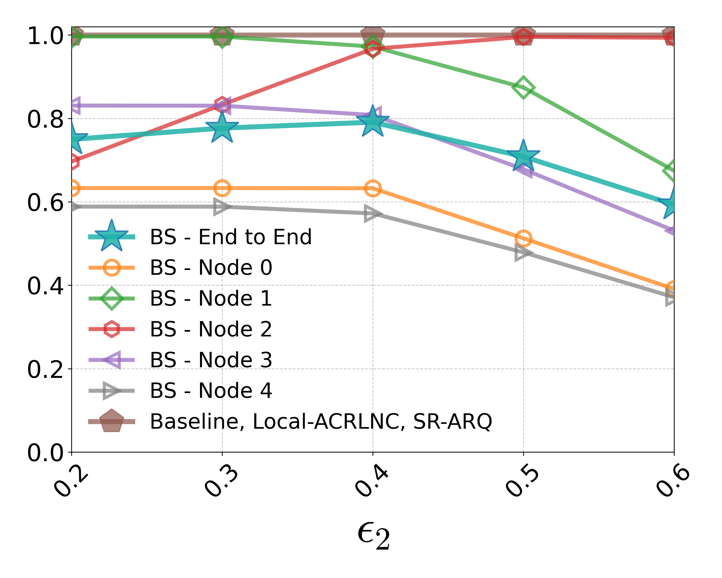
(a) Channel Usage Rate - $U,U_{n}$

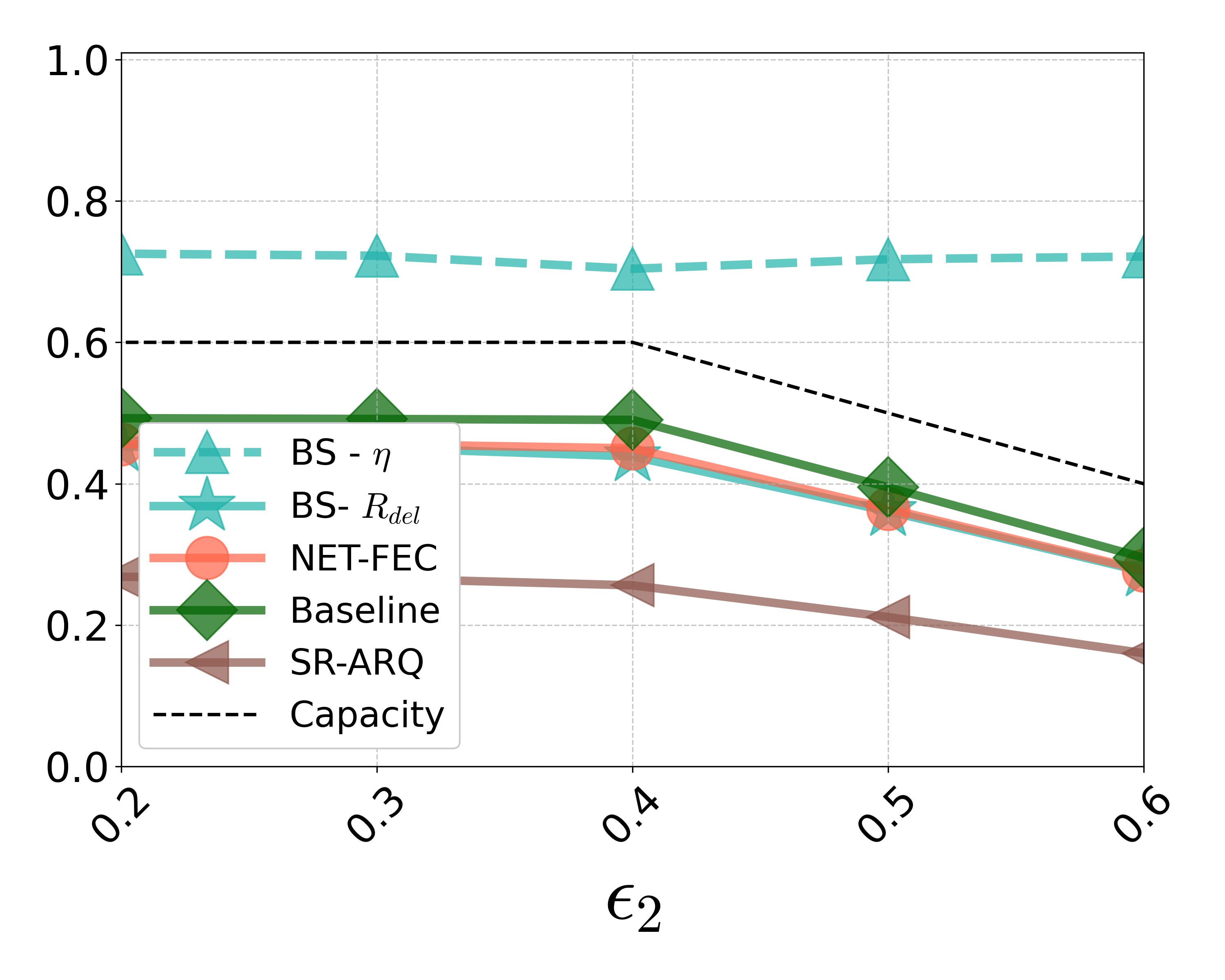
(b) $R_{\rm del}$ and $\eta$

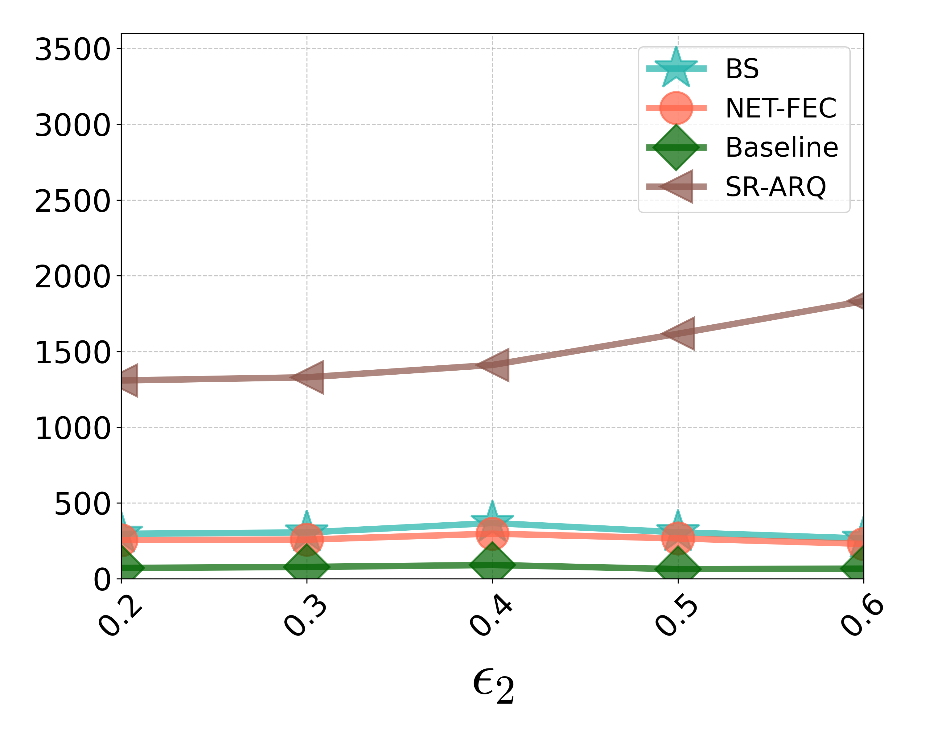
(c) Mean Delay [Slots] - $D^{\rm mean}$

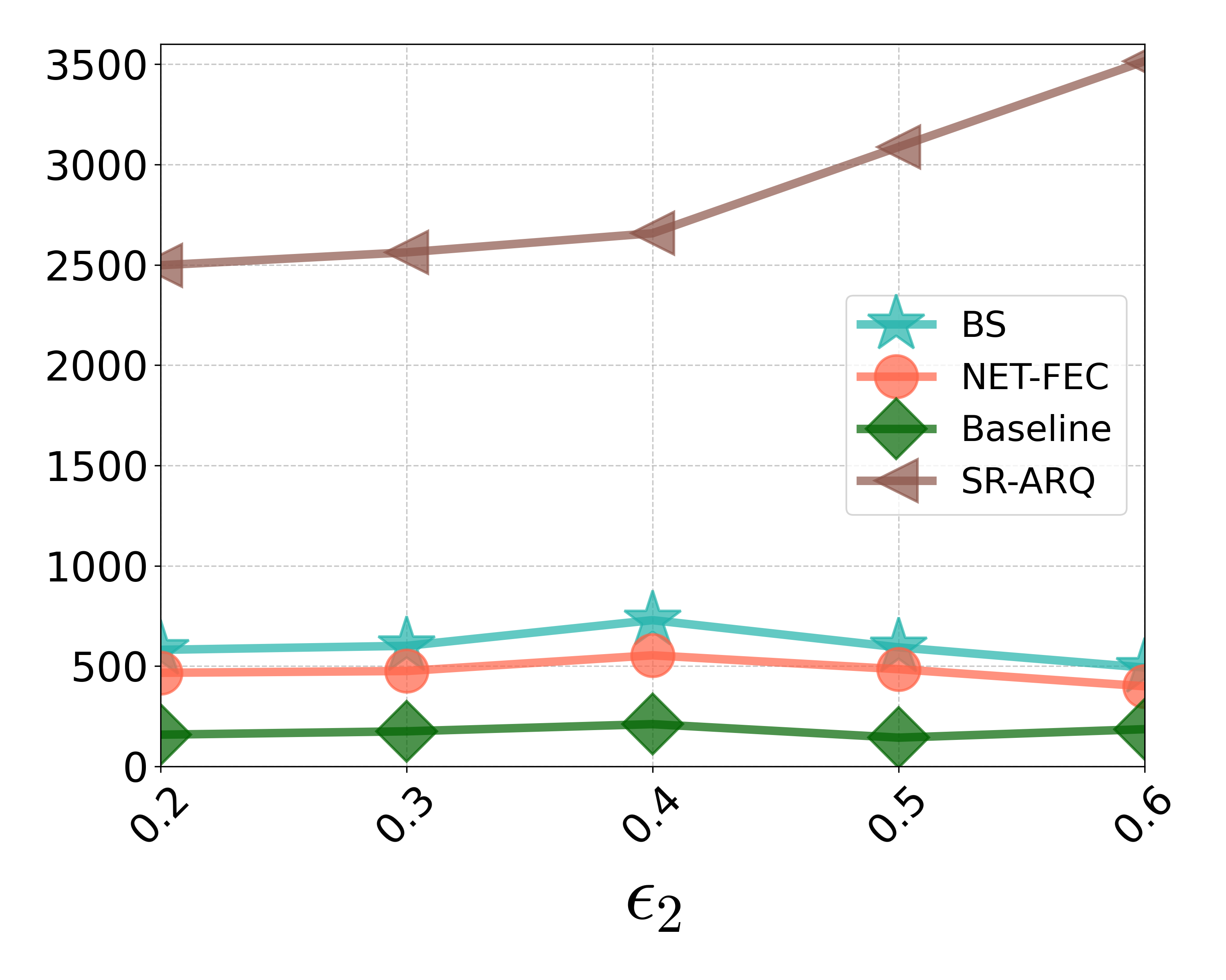
(d) Max Delay [Slots] - $D^{\rm max}$

Figure 3: System performance of 6-nodes network with respect to $\epsilon_{2}$ where $\epsilon_{0}=\epsilon_{5}=0.1$, $\epsilon_{2}=0.4$.

1. BSP Duration: The BSP duration is determined based on the a priori FEC periods of subsequent nodes in the network and considering the following: 1) While nodes transmit FEC relative to their newly transmitted DoFs ($c_{t}^{\text{new}}$, M1), this information isn’t directly available through feedback links. However, estimation of the subsequent links’ erasure rates is available by backward feedback aggregation $AF^{n}_{t}$ (lines 1-2). That is, the destination node sends back an ACK/NACK message to node N-1, which in turn sends back two things: its own feedback message, along with the feedback message it received from the destination. Then node N-1 sends both messages to node N-2, which adds its own feedback and passes all three messages back. This process continues backwards through the chain, where each node sends back its own feedback message $F^{n}_{t}$ and the collection of messages it received from the next node denoted by $AF^{n}_{t}$. Specifically, $AF^{n}_{t}$ contains acknowledgments $F_{t^{\prime}}^{i}$ from nodes $n+1$ to $N-1$ at times $t^{\prime}$ not exceeding $t-\sum_{k=i}^{N-1}\rm RTT_{k}$. The erasure rate of each preceding channel $\hat{\epsilon}_{n}$ is then computed as the mean of all its corresponding acknowledgments in $AF^{n}_{t}$ by (2). 2) The forward-channels bottleneck link, which requires the highest FEC transmission, constrains the local theoretical capacity and contributes the most BSP slots. Any packet at this link should be forwarded immediately to maintain high transmission rates, regardless of subsequent channel conditions. Therefore, the BSP duration considers two factors: the basic window of new DoFs for each $i$th hop - $\rm RTT_{i}$, and the estimated erasure rates up to the forward bottleneck, resulting, for node $n$ at time $t$ as

   $$\textstyle BS_{n}(t)=\begin{cases}\textstyle\alpha\sum_{i=n+1}^{BN_{n}}\rm RTT_{i}\cdot\hat{\epsilon}_{i}&\hskip-5.69046pt\text{if }n<BN_{n},\text{ using Eq.\hskip-2.84544pt~\eqref{eqn: BN_n}}\\ \textstyle 0&\hskip-5.69046pt\text{if }n=BN_{n}\end{cases}$$ (9)

   where $\alpha$ is a tuneable parameter used to relax the evaluation error. Note that if channel $e_{n}$ is the forward bottleneck itself, we set $BS_{n}(t)=0$, eliminating any transmission suspension.

2. BS Termination Criterion: Transmission suspension can be considered a packet erasure, allowing us to analyze this through the DoF rate framework given in (8). We want to identify the critical point where further suspension would degrade the data rate performance. To model this, we set $md_{t}^{\text{nack}}=1$, representing guaranteed packet erasure, with the remaining BSP window available for re-transmissions compensation. Since only FEC are considered, $c_{t}^{\text{new}}=0$, and with uncertain delivery, $ad_{t}^{\text{ack}}=0$. Finally, $c_{t}^{\text{same}}=BS_{n}(t)$, representing the number of re-transmissions with unknown delivery status. While a node’s transmission rate is constrained by its forward channels bottleneck, channels with similar erasure rates can have significant impact as well. To quantify this, we consider both the erasure rate differential between the current channel and its bottleneck, and their distance in hops, denoted by $h=BN_{n}-n$. This sets the BSP-DoF rate by

   $$\textstyle\Delta_{t}^{BS}=\left[\left(1-\hat{\epsilon}_{n}\right)BS(t)+h\log(\hat{\epsilon}_{BN_{n}}-\hat{\epsilon}_{n})\right]^{-1}.$$

   To ensure suspending transmission doesn’t reduce the rate below the capacity, we compare the BSP DoF rate to the forward bottleneck rate. Thus, the BSP is terminated when,

   $$\textstyle\Delta_{t}^{BS}>1-\hat{\epsilon}_{BN_{n}}.$$ (10)

   This criterion identifies the critical point where the remaining transmission slots, $BS_{n}(t)$, are the slots needed to compensate for the "missing" DoF. Any further pause would likely result in a rate reduction.

IV Evaluation Results

In this section, we present simulation results demonstrating the effectiveness of the BS protocol . We evaluate a 6-node network with BEC channels, where $\epsilon_{0}=\epsilon_{5}=0.1$, $\epsilon_{1}=0.4$, $\epsilon_{3}=0.3$, and middle link $\epsilon_{2}$ varies from $0.2$ to $0.6$ across simulations. The global bottleneck remains $\epsilon_{BN}=\epsilon_{1}=0.4$ until $\epsilon_{2}$ exceeds $0.4$ and becomes the global bottleneck itself. Considering the capacity limit, information packets arrive at the source according to a Bernoulli process with a rate slightly lower than the global bottleneck, $1-\epsilon_{BN}-0.1$. We set $\rm RTT_{n}=20$ for each node $n$, yielding a global $\rm RTT$ of $100$ slots over a time horizon of $T=5000$ slots. We compare four algorithms: 1) The proposed BS (’BS’). 2) ’NET-FEC’, a BS version which performs NET without idle periods - the BS period is eliminated and No-New No-FEC pauses are replaced with FEC transmissions - This allows us to evaluate the effect of the idle periods distinctively. 3) ’Baseline’ using MP-MH AC-RLNC, implementing AC-RLNC only at the source with basic re-encoding at intermediate nodes (see Sec. II-C2); and 4) common non-coded selective repeat ARQ (’SR-ARQ’) [33]. In Fig. 3, we present the channel usage savings compared to the rate and delay metrics. In Fig.3(a), we present the channel usage rate for each node separately and for the end-to-end network (5). While NET-FEC, Baseline, and SR-ARQ operate at maximum channels utilization (rate of 1), BS achieves significant reductions Examining each node, channel usage typically decreases as the global bottleneck becomes more severe and shifts position at $\epsilon_{2}\geq 0.4$, demonstrating how BS nodes adapt to network bottleneck constraints. Node $2$, however, shows distinct behavior: its activity increases with its erasure rate, reaching maximum utilization when it becomes the bottleneck. The end-to-end performance (blue stars) reveals that overall channel usage decreases with increasing erasure rate, highlighting BS’s network-level benefits. We observe a $20\%$ reduction in channel usage when $\epsilon_{1}=0.4$ is the bottleneck, with even greater efficiency gains as the bottleneck shifts across the network. In Fig. 3(b), we present goodput and delivery rates. The metrics are nearly identical (within $0.01$) for all algorithms except BS, and are thus given by a single line. BS shows significantly higher goodput, indicated by the dashed line with upward triangles, due to its transmission pauses. Notably, BS reduces channel usage, while maintaining a delivery rate comparable to the coding algorithms and outperforms the SR-ARQ. This demonstrates the algorithm does not compromise its delivery performance for reducing channel usage. The in-order delivery delay metrics of all the AC-RLNC solutions are upper-bounded in mean and max metrics by $400$ and $750$ time slots, respectively. The overall difference between the compared solutions remains within approximately two global $\rm RTT$. As demonstrated in [25], these delays meet the standard requirements for URLLC, and are one-order better than rateless RLNC [34], and two-orders better than non-coded solutions with UDP and selective repeat ARQ [33], which are typically used in TCP layers (discussed also in [25, 23, 22]). In Fig 4 we present a single-source multicast scenario where all intermediate nodes function as destinations, decoding the information packets. Note that this decoding does not affect the algorithm’s operation, which continues to function in its original semi-decoding manner. The results for both BS and NET-FEC demonstrate how delay varies with respect to the bottleneck channel position. The first node (Fig 4(a)) experiences a minimal delay, consistent with the expected AC-RLNC algorithm performance. At the second node (Fig 4(b)), we observe two distinct behaviors: high delay when $\epsilon\leq 0.4$ due to transmission over the bottleneck channel, and low delay when $\epsilon>0.4$ as the bottleneck shifts further downstream in the network. The remaining nodes (Fig 4(c)-Fig 4(e)) exhibit higher delays as they are all affected by the bottleneck channel. The goodput and delivery rate results align with our multi-hop findings (Fig 2). These metrics remain consistent across nodes since all algorithms consider the end-to-end network conditions rather than local information. While the delivery rate shows a slight decrease with distance from the source due to cumulative erasures, this could be improved through better erasure rate estimation. The baseline solution demonstrates stable rate and delay performance due to its global approach, though at the cost of higher channel usage as shown in Fig. 3(a). While SR-ARQ achieves competitive performance at the first node, its performance degrades significantly at subsequent nodes. Unlike the coding solutions, which consider the entire 6-node network, SR-ARQ operates locally at each node. This leads to high delivery rates at the initial nodes but declining performance when reaching bottleneck nodes. Since the multicast scenario requires uniform delivery rates across all nodes, this initial advantage becomes irrelevant. Each channel usage rate is seen in (Fig 2). These results demonstrate that BS achieves significant improvements in channel usage and goodput while maintaining baseline delivery rate and low delay performance, validating the effectiveness of the proposed approach.

Future Work and Discussion: Based on these promising results, we propose two key directions for further investigation. Investigating varying RTTs between nodes could improve our approach by allowing nodes with faster connections to pause while waiting for slower channels. Extending to multipath-multihop scenarios would also enable smarter transmission scheduling through idle nodes, enhancing network efficiency.

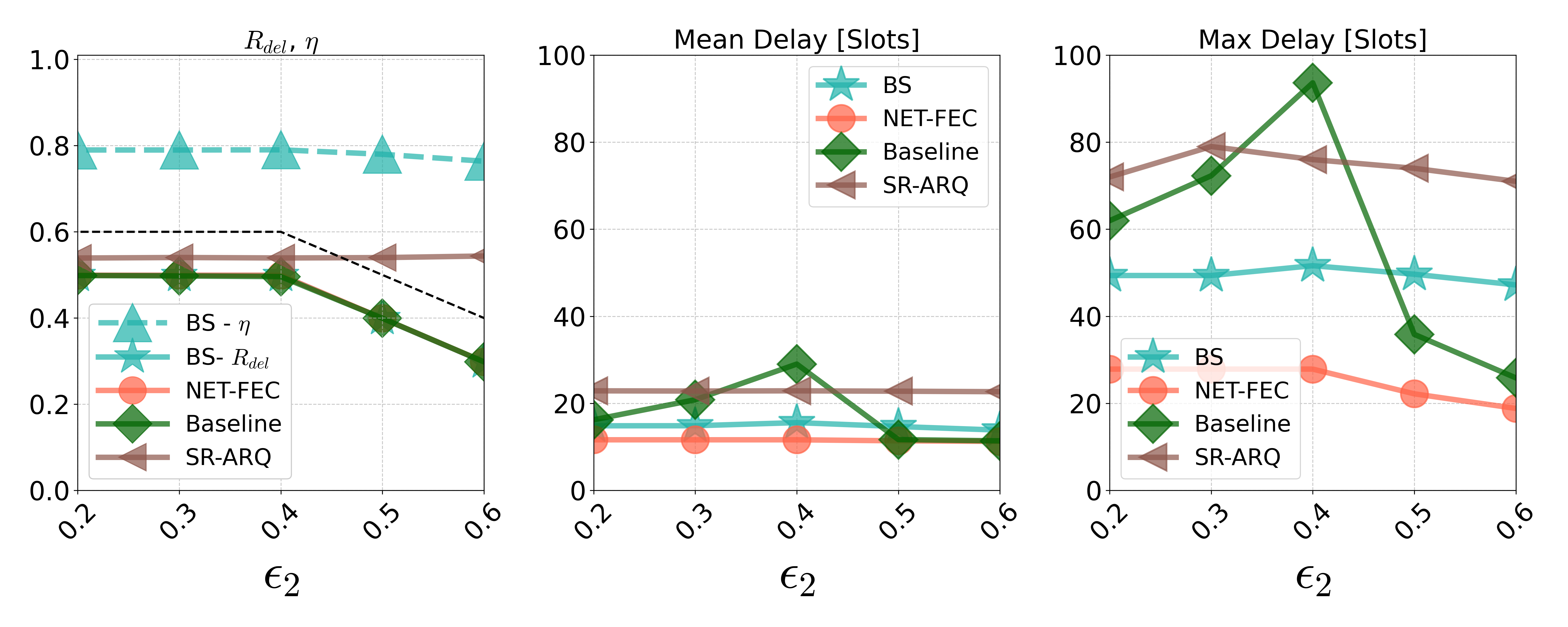
(a) Node 1. The capacity for SR-ARQ is 0.9.

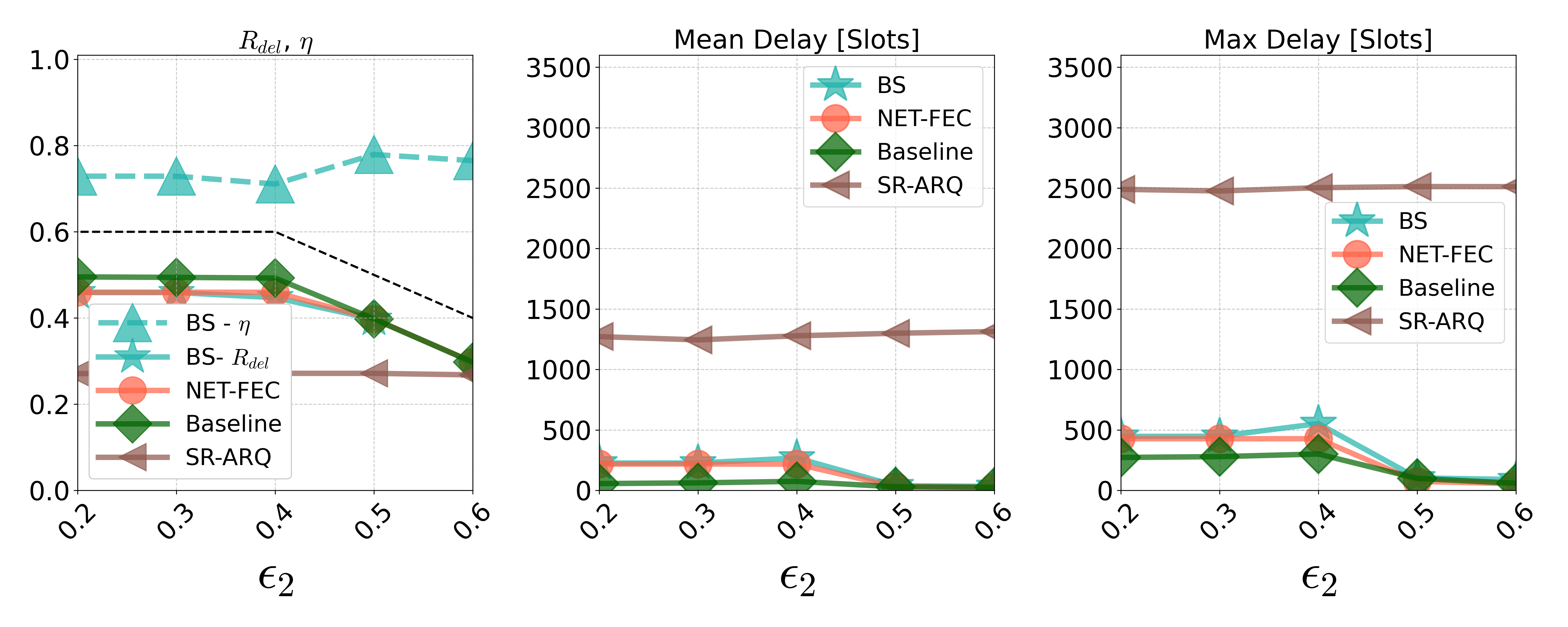
(b) Node 2. The capacity for SR-ARQ is 0.6.

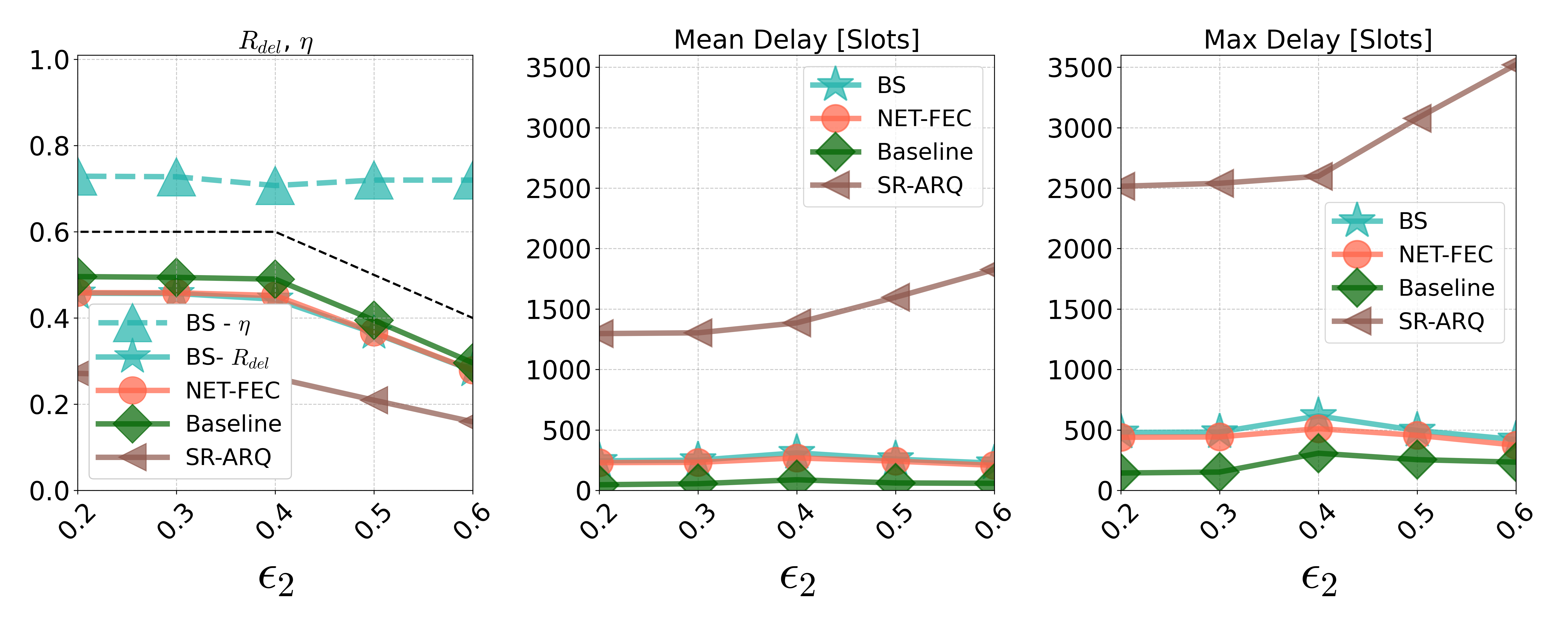
(c) Node 3. The capacity for SR-ARQ is $\epsilon_{2}$.

(d) Node 4. The capacity for SR-ARQ is $\epsilon_{2}$.

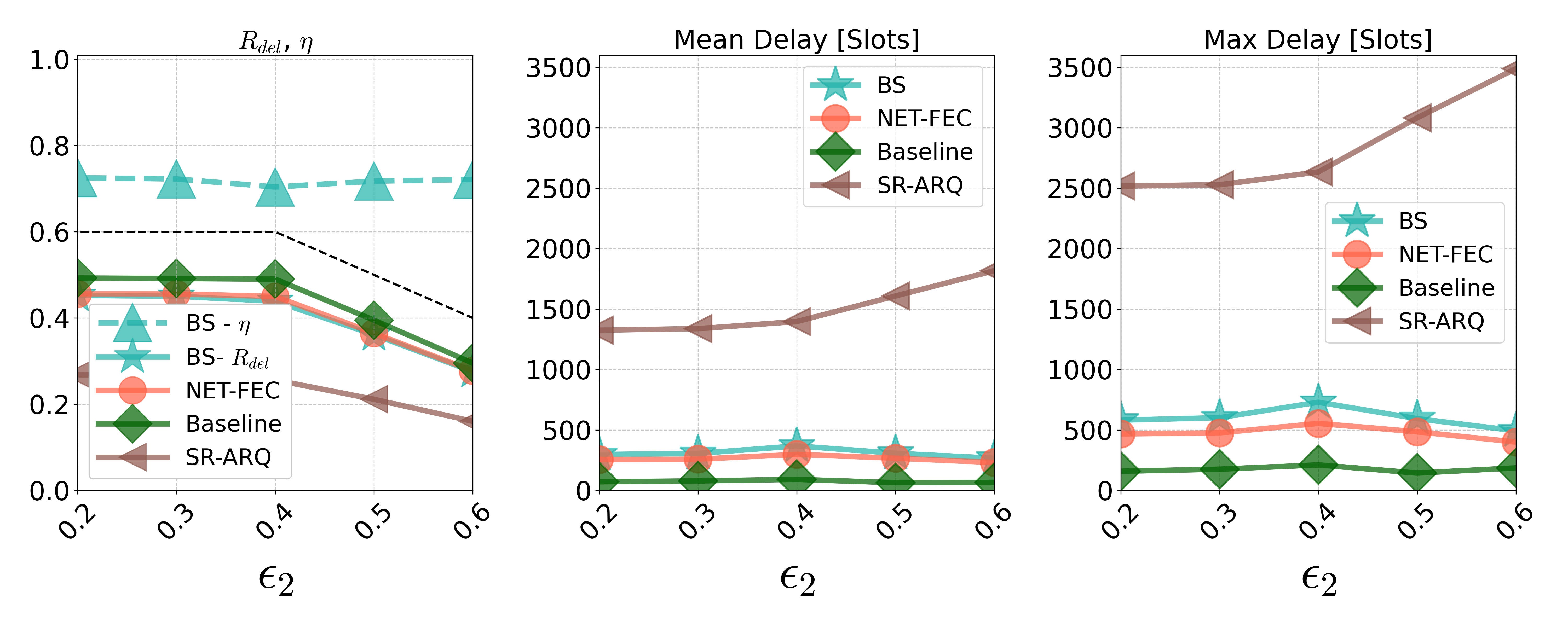
(e) Node 5. The capacity for SR-ARQ is $\epsilon_{2}$.

Figure 4: Analysis of multi-cast Scenario when all nodes function as destinations.

References

- [1] E. Yanmaz, S. Yahyanejad, B. Rinner, H. Hellwagner, and C. Bettstetter, “Drone networks: Communications, coordination, and sensing,” Ad Hoc Networks, vol. 68, pp. 1–15, 2018.
- [2] M. Kumar and R. Mishra, “An overview of MANET: History, challenges and applications,” Indian Journal of Computer Science and Engineering (IJCSE), vol. 3, no. 1, pp. 121–125, 2012.
- [3] M. Radi, B. Dezfouli, K. A. Bakar, and M. Lee, “Multipath routing in wireless sensor networks: survey and research challenges,” sensors, vol. 12, no. 1, pp. 650–685, 2012.
- [4] S.-Y. Li, R. W. Yeung, and N. Cai, “Linear network coding,” IEEE transactions on information theory, vol. 49, no. 2, pp. 371–381, 2003.
- [5] R. Ahlswede, N. Cai, S.-Y. Li, and R. W. Yeung, “Network information flow,” IEEE Transactions on information theory, vol. 46, no. 4, pp. 1204–1216, 2000.
- [6] T. Ho, M. Médard, R. Koetter, D. R. Karger, M. Effros, J. Shi, and B. Leong, “A random linear network coding approach to multicast,” IEEE Transactions on information theory, vol. 52, no. 10, pp. 4413–4430, 2006.
- [7] M. Luby, “LT codes,” in The 43rd Annual IEEE Symposium on Foundations of Computer Science, 2002. Proceedings. IEEE Computer Society, 2002, pp. 271–271.
- [8] A. Shokrollahi, “Raptor codes,” IEEE transactions on information theory, vol. 52, no. 6, pp. 2551–2567, 2006.
- [9] G. Joshi, Y. Kochman, and G. W. Wornell, “On playback delay in streaming communication,” in 2012 IEEE International Symposium on Information Theory Proceedings. IEEE, 2012, pp. 2856–2860.
- [10] J. Cloud, D. Leith, and M. Médard, “A coded generalization of selective repeat ARQ,” in 2015 IEEE Conference on Computer Communications (INFOCOM). IEEE, 2015, pp. 2155–2163.
- [11] F. Gabriel, A. K. Chorppath, I. Tsokalo, and F. H. Fitzek, “Multipath communication with finite sliding window network coding for ultra-reliability and low latency,” in 2018 IEEE International Conference on Communications Workshops (ICC Workshops). IEEE, 2018, pp. 1–6.
- [12] E. Tasdemir, V. Nguyen, G. T. Nguyen, F. H. P. Fitzek, and M. Reisslein, “FSW: Fulcrum Sliding Window Coding for Low-Latency Communication,” IEEE Access, vol. 10, pp. 54 276–54 290, 2022.
- [13] J. Du, N. Sweeting, D. C. Adams, and M. Médard, “Network reduction for coded multiple-hop networks,” in 2015 IEEE International Conference on Communications (ICC), 2015, pp. 4518–4523.
- [14] D. Malak, M. Médard, and E. M. Yeh, “Tiny codes for guaranteeable delay,” IEEE Journal on Selected Areas in Communications, vol. 37, no. 4, pp. 809–825, 2019.
- [15] D. Malak, A. Schneuwly, M. Médard, and E. Yeh, “Delay-aware coding in multi-hop line networks,” in 2019 IEEE 5th World Forum on Internet of Things (WF-IoT), 2019, pp. 650–655.
- [16] Y. Shi, Y. E. Sagduyu, J. Zhang, and J. H. Li, “Adaptive coding optimization in wireless networks: Design and implementation aspects,” IEEE Transactions on Wireless Communications, vol. 14, no. 10, pp. 5672–5680, 2015.
- [17] G. Kasper Facenda, E. Domanovitz, M. Nikhil Krishnan, A. Khisti, S. L. Fong, W.-T. Tan, and J. Apostolopoulos, “On state-dependent streaming erasure codes over the three-node relay network,” in 2022 IEEE International Symposium on Information Theory (ISIT), 2022, pp. 1951–1956.
- [18] E. Domanovitz, A. Khisti, W.-T. Tan, X. Zhu, and J. Apostolopoulos, “Streaming erasure codes over multi-hop relay network,” in 2020 IEEE International Symposium on Information Theory (ISIT), 2020, pp. 497–502.
- [19] S. L. Fong, A. Khisti, B. Li, W.-T. Tan, X. Zhu, and J. Apostolopoulos, “Optimal streaming erasure codes over the three-node relay network,” IEEE Transactions on Information Theory, vol. 66, no. 5, pp. 2696–2712, 2020.
- [20] G. K. Facenda, M. N. Krishnan, E. Domanovitz, S. L. Fong, A. Khisti, W.-T. Tan, and J. Apostolopoulos, “Adaptive relaying for streaming erasure codes in a three node relay network,” IEEE Transactions on Information Theory, vol. 69, no. 7, pp. 4345–4360, 2023.
- [21] A. Cohen, D. Malak, V. B. Bracha, and M. Médard, “Adaptive causal network coding with feedback,” IEEE Transactions on Communications, vol. 68, no. 7, pp. 4325–4341, 2020.
- [22] A. Cohen, G. Thiran, V. B. Bracha, and M. Médard, “Adaptive causal network coding with feedback for multipath multi-hop communications,” IEEE Transactions on Communications, vol. 69, no. 2, pp. 766–785, 2020.
- [23] A. Cohen, H. Esfahanizadeh, B. Sousa, J. P. Vilela, M. Luis, D. Raposo, F. Michel, S. Sargento, and M. Medard, “Bringing network coding into SDN: Architectural study for meshed heterogeneous communications,” IEEE Communications Magazine, vol. 59, no. 4, pp. 37–43, 2021.
- [24] A. Cohen, M. Médard, and S. S. Shitz, “Broadcast approach meets network coding for data streaming,” in 2022 IEEE International Symposium on Information Theory (ISIT). IEEE, 2022, pp. 25–30.
- [25] E. Dias, D. Raposo, H. Esfahanizadeh, A. Cohen, T. Ferreira, M. Luís, S. Sargento, and M. Médard, “Sliding window network coding enables NeXt generation URLLC millimeter-wave networks,” IEEE Networking Letters, vol. 5, no. 3, pp. 159–163, 2023.
- [26] R. Ali, Y. B. Zikria, A. K. Bashir, S. Garg, and H. S. Kim, “URLLC for 5G and beyond: Requirements, enabling incumbent technologies and network intelligence,” IEEE Access, vol. 9, pp. 67 064–67 095, 2021.
- [27] T. M. Cover and J. A. Thomas, Elements of Information Theory, 2nd ed. New-York: Wiley, 2006.
- [28] D. Malak, M. Médard, and E. M. Yeh, “Tiny codes for guaranteeable delay,” IEEE J. Sel. Areas in Commun., vol. 37, no. 4, Apr. 2019.
- [29] D. S. Lun, M. Médard, R. Koetter, and M. Effros, “On coding for reliable communication over packet networks,” Physical Communication, vol. 1, no. 1, pp. 3–20, 2008.
- [30] P. Karafillis, K. Fouli, A. ParandehGheibi, and M. Médard, “An algorithm for improving sliding window network coding in tcp,” 03 2013, pp. 1–5.
- [31] F. Michel, A. Cohen, D. Malak, Q. De Coninck, M. Médard, and O. Bonaventure, “FlEC: Enhancing QUIC with application-tailored reliability mechanisms,” 2022.
- [32] A. Cohen, A. Solomon, and N. Shlezinger, “DeepNP: Deep Learning-Based Noise Prediction for Ultra-Reliable Low-Latency Communications,” in 2022 IEEE International Symposium on Information Theory (ISIT), 2022, pp. 2690–2695.
- [33] E. Weldon, “An improved selective-repeat ARQ strategy,” IEEE Transactions on Communications, vol. 30, no. 3, pp. 480–486, 1982.
- [34] N. Bonello, Y. Yang, S. Aissa, and L. Hanzo, “Myths and realities of rateless coding,” IEEE Communications Magazine, vol. 49, no. 8, pp. 143–151, 2011.