On a Semiparametric Stochastic Volatility Model

Abstract

This paper presents a novel approach to stochastic volatility (SV) modeling by utilizing nonparametric techniques that enhance our ability to capture the volatility of financial time series data, with a particular emphasis on the non-Gaussian behavior of asset return distributions. Although traditional parametric SV models can be useful, they often suffer from restrictive assumptions regarding errors, which may inadequately represent extreme values and tail behavior in financial returns. To address these limitations, we propose two semiparametric SV models that use data to better approximate error distributions. To facilitate the computation of model parameters, we developed a Markov Chain Monte Carlo (MCMC) method for estimating model parameters and volatility dynamics. Simulations and empirical tests on S$\&$P 500 data indicate that nonparametric models can minimize bias and variance in volatility estimation, providing a more accurate reflection of market expectations about volatility. This methodology serves as a promising alternative to conventional parametric models, improving precision in financial risk assessment and deepening our understanding of the volatility dynamics of financial returns.

Keywords: Stochastic Volatility Model, Bayesian Inference, MCMC, Semiparametric, Nonparametric, Volatility, Financial time series.

1 Introduction

In the realm of financial time series analysis, the volatility of asset returns occupies a central position. The significance of volatility modeling extends across a broad spectrum of practical financial applications, encompassing asset pricing, portfolio optimization, and risk management, among others. Given its pivotal role over three decades, a significant effort has been made in financial literature to research and develop methods for estimating volatility. Prominent among these modeling techniques are the Auto-regressive Conditional Heteroskedasticity (ARCH) model, pioneered by Engle, (1982), the Generalized ARCH (GARCH) model by Bollerslev, (1986), and the Stochastic Volatility (SV) Model, which was conceptualized by Taylor, (1994). In particular, the Taylor style model of returns $y_{1},y_{2},...,y_{N}$ is

$$y_{t} =\sqrt{h_{t}}u_{t},\ t=1,...,N$$ (1)

$$\ln h_{t} =\alpha+\delta\ln h_{t-1}+\sigma_{\nu}\nu_{t},\ t=2,...,N$$

where $u_{t},\nu_{t}\sim N(0,1)$ for $t=1,...,N$ and $corr(u_{t},\nu_{t^{\prime}})=0$ for all $t$ and $t^{\prime}$.

Further studies on similar model frameworks have been conducted by various researchers, including Hull and White, (1987), Chesney and Scott, (1989), Taylor, (1994), Doan et al., (1994), Eric Jacquier and Rossi, (2002), and Shephard, (1996). Their works delve deeper into the methods for both parametric and semi-parametric estimation of stochastic volatility models. Harvey and Shephard, (1996) introduced an asymmetric stochastic volatility model that incorporates the leverage effect, utilizing a quasi-maximum likelihood estimation approach within a state-space framework, which facilitates the analysis of financial time series displaying asymmetric volatility patterns. Carter and Kohn, (1994) developed a Gibbs sampling technique for examining state-space models, particularly effective in cases where errors are governed by mixture distributions and coefficients evolve over time. Kim et al., (1998) suggested a Bayesian approach using MCMC methods for stochastic volatility models, highlighting the advantages of SV models over ARCH models in representing the volatility dynamics of financial time series while introducing methods for filtering, diagnostics, and model selection. In addition, Omori et al., (2007) broadened the Bayesian analysis of SV models to account for leverage effects and presented a robust MCMC-based technique that employs a mixture approximation for the joint innovation distributions.

In financial econometrics, Taylor’s Stochastic Volatility Model (SVM) offers the notable advantage of accommodating time-varying volatility. However, as critiqued by Durham, (2006), the model is hindered by its inability to encapsulate the commonly observed heavy-tailed behavior in the conditional distribution of returns. This shortcoming stems from its Gaussian assumption for the error terms. A central objective within financial econometrics is examining the returns distribution from financial markets, which yields insights into the mechanisms propelling financial dynamics. Mandelbrot, (1963) on cotton price fluctuations revealed pronounced heavy-tailedness compared to normal distributions, prompting the exploration of stable distributions as a superior alternative to conventional Gaussian distribution models.

To tackle this issue, alternative parametric heavy-tailed distributions like the Student’s t distribution with low degrees of freedom or the Generalized Error Distribution (GED) are options to explore. Nonetheless, as highlighted in the articles by Di and Gangopadhyay, (2011), Di and Gangopadhyay, (2013), when the actual error distribution is not known, these parametric assumptions frequently fall short. They often fail to capture the structural behavior of financial data accurately.

One possible solution to this constraint is to utilize a non-parametric distribution for the return error term. This approach would offer increased flexibility in capturing the empirical characteristics of financial data, effectively allowing the data to “speak for itself” Similar concepts have been explored in prior research by Di and Gangopadhyay, (2013) and Di and Gangopadhyay, (2011) concerning GARCH models. The authors introduced a novel method for nonparametrically estimating the error distribution, which led to the development of a pseudo-likelihood function for the model. The resulting volatility derives from the GARCH parameters estimated via this likelihood.

In this paper, we propose a similar semiparametric approach to estimating volatility based on the SVM. However, the problem is significantly more challenging compared to the semiparametric formulation of GARCH. First, the SVM model introduced in Equation 1 requires the specification of the error distributions for both the observation equation $u_{t}$ and the volatility equation $\nu_{t}$. Therefore, the semiparametric SVM introduced in this paper involves a novel methodology to utilize the latent features of the model to develop nonparametric estimates of the error terms. Second, the resulting pseudo-likelihood poses a significant optimization problem requiring a computational solution. Therefore, in the pursuit of constructing a semiparametric model, the deployment of numerical methods becomes vital. This paper discusses a computational solution based on the Markov Chain Monte Carlo (MCMC) technique for SV models rooted in the pioneering work by Jacquier et al., (2004). This foundational work introduces Bayesian inference mechanisms for conventional parametric SVM discussed in Equation 1.

The approach utilized in this paper involves a two-step process. We begin by fitting an initial parametric model; the derived volatility estimate is denoted by $\hat{h}$. Subsequently, the initial residual $\hat{u_{t}}$ can be defined as $y_{t}/\hat{h}$, which can be used to develop a kernel density estimate $f$, the pdf of the error term $u_{t}$. Based on the resulting estimate, $\hat{f}$, along with a parametric assumption on the volatility error term $\nu_{t}$, it becomes feasible to fit the semiparametric SVM model employing analogous sampling techniques.

However, the ultimate objective of the current work is to develop a full semiparametric framework of the SVM. Towards this goal, we propose an approach to jointly estimate the density of the error terms $u_{t}$ and $\nu_{t}$. This is done by recursively approximating the residual of the observation equation as described earlier, along with the residual term from the volatility equation, denoted as $w_{t}$, i.e., $w_{t}=\frac{\ln h_{t}-u_{t}}{\sigma}$, which is utilized to estimate $g$, the pdf of the volatility noise $\nu_{t}$.

This methodology parallels our treatment of the initial residual, wherein we employ kernel density estimation to approximate the error distribution for both residuals. Consequently, in addition to $f$, the function $g$ is utilized as the standardized version of the kernel density estimate of $\frac{w_{t}-mean(w_{t})}{sd(w_{t})}$. Embracing this semiparametric paradigm, the comprehensive model can be effectively operationalized within a Bayesian framework, employing Markov Chain Monte Carlo (MCMC) techniques to facilitate its implementation.

The advantage of the semiparametric model can be proved by comparing it to its parametric counterpart. This comparative analysis was facilitated using simulated data sets featuring both normally distributed innovations and those with heavy-tailed innovations, such as the Student’s t distribution and the Generalized Error Distribution (GED). Additionally, empirical data from the S$\&$P 500 was also utilized in this endeavor. The resultant findings elucidate that the non-parametric model boasts a reduced variance coupled with an amplified precision in parameter estimation.

The rest of the paper is organized as follows: Section 2 introduces MCMC sampling in the context of the MCMC sampling scheme utilized in the paper; sections 3 and 4 contain the key contribution of the paper by proposing the pseudo-likelihood of the semiparametric SVM and a Bayesian MCMC methodology to estimate the model parameters and resulting volatility. Sections 3 and 4 illustrate the proposed model’s performance via extensive simulation and an analysis of the S&P 500 dataset. The paper concludes with a discussion of the implications of the results.

2 Semiparametric Estimation in Stochastic Volatility Model

This section will introduce the concept and related computational tools for semiparametric SVM. However, in the next subsection, we will first review a Bayesian framework for SVM and the related computational tools.

2.1 A Bayesian framework of SVM

The Taylor-style stochastic volatility model is

$$y_{t}=\sqrt{h_{t}}u_{t},\ t=1,...,N$$ (2)

$$\ln h_{t}=\alpha+\delta\ln h_{t-1}+\sigma_{\nu}\nu_{t},\ t=2,...,N$$ (3)

At a given $t=1,...,N$, the return from holding a financial asset equals $y_{t}$ and the latent log volatility $h_{t}$ follows the first-order auto-regressive process with $\delta$, $\alpha$ and $\sigma_{\nu}$ parameters, where $\alpha$ is the intercept parameter, $\delta$ is the volatility persistence and $\sigma_{\nu}$ is the standard deviation of the shock to the logarithm of $h_{t}$.

This particular form of the model has been employed in studies by Taylor, (1994), Hull and White, (1987), Chesney and Scott, (1989), Shephard, (1996), Ghysels et al., (1996), Doan et al., (1994), Kim et al., (1998). The works mentioned above extensively discuss the fundamental econometric characteristics of the model, as well as the estimation procedures for Stochastic Volatility models.

Following the work of Doan et al., (1994), the joint unconditional distribution including $y_{t}$, $h_{t}$, $\delta$, $\alpha$, $\sigma_{\nu}$ is

$$p(y,h,\delta,\alpha,\sigma_{\nu}^{2})\propto \frac{1}{\sigma_{\nu}^{\nu_{0}}\sigma_{\delta}\sigma_{\alpha}\sigma_{\nu}^{2}}\exp(-\frac{(\delta-\delta_{0})^{2}}{2\sigma_{\delta}^{2}}-\frac{(\alpha-\alpha_{0})^{2}}{2\sigma_{\alpha}^{2}}-\frac{s_{0}^{2}}{2\sigma_{\nu}^{2}})$$ (4)

$$\times\prod_{t=2}^{N}\frac{1}{\sqrt{h_{t}}h_{t}\sigma_{\nu}}\exp(-\frac{y_{t}^{2}}{2h_{t}}-\frac{(\ln h_{t}-\delta\ln h_{t-1}-\alpha)^{2}}{2\sigma^{2}_{\nu}})$$

From this joint distribution, we can derive the posterior distributions of $\delta$, $\alpha$, $\sigma_{\nu}$:

$$p(\sigma_{\nu}^{2}|h,\alpha,\delta)\sim IG\left(\frac{\nu_{0}+N-1}{2},\frac{s}{2}\right)$$ (5)

$$p(\delta|h,\alpha,\sigma_{\nu}^{2})\sim N\left(\frac{\sigma_{\nu}^{2}\delta_{0}+\sigma_{\delta}^{2}s_{3}-\sigma_{\delta}^{2}\alpha s_{1}+\sigma_{\delta}^{2}\alpha\ln h_{N}}{\sigma_{\nu}^{2}+\sigma_{\delta}^{2}s_{2}-\sigma_{\delta}^{2}(\ln h_{N})^{2}},\frac{\sigma_{\nu}^{2}\sigma_{\delta}^{2}}{\sigma_{\nu}^{2}+\sigma_{\delta}^{2}(s_{2}-(\ln h_{N})^{2})}\right)$$ (6)

$$p(\alpha|h,\sigma_{\nu}^{2},\delta)\sim N\left(\frac{\sigma_{\nu}^{2}\alpha_{0}+\sigma_{\alpha}^{2}(1-\delta)s_{1}-\sigma_{\alpha}^{2}\ln h_{1}+\sigma_{\alpha}^{2}\delta\ln h_{N}}{\sigma_{\nu}^{2}+N\sigma_{\alpha}^{2}-\sigma_{\alpha}^{2}},\frac{\sigma_{\nu}^{2}\sigma_{\alpha}^{2}}{\sigma_{\nu}^{2}+N\sigma_{\alpha}^{2}-\sigma_{\alpha}^{2}}\right)$$ (7)

where $s=s_{0}+(N-1)\alpha^{2}+(1+\delta^{2})s_{2}-\delta^{2}(\ln h_{N})^{2}-(\ln h_{1})^{2}-2\alpha s_{1}\delta+2\alpha\ln h_{1}-2\alpha\delta\ln h_{N}-2\delta s_{3}$, $s_{1}=\sum_{t=1}^{N}\ln h_{t}$, $s_{2}=\sum_{t=1}^{N}(\ln h_{t})^{2}$, $s_{3}=\sum_{t=2}^{N}\ln h_{t}\ln h_{t-1}$.

The conditional posterior of $h_{t}$ is

$$p(h_{t}|h_{t+1},h_{t-1},\delta,\alpha,\sigma_{\nu}^{2})\propto\frac{1}{\sqrt{h_{t}}}\exp\left(-\frac{y_{t}^{2}}{2h_{t}}\right)\frac{1}{h_{t}}\exp\left(-\frac{(\ln h_{t}-\mu_{t})^{2}}{2\sigma^{2}}\right)$$ (8)

where

$$\mu_{t}=\frac{\delta(\ln h_{t+1}+\ln h_{t-1})+\alpha(1-\delta)}{1+\delta^{2}},\sigma^{2}=\frac{\sigma_{\nu}^{2}}{1+\delta^{2}}$$ (9)

In conventional parametric SVM, the error terms, $u_{t}$ and $\nu_{t}$, are typically assumed to follow independent normal distributions, a presumption that has been increasingly scrutinized and challenged in contemporary literature. For example, Omori et al., (2007) and Jacquier et al., (2004) have proposed using a t-distribution. Similarly, Barndorff-Nielsen, (1997) introduced the Normal-Inverse Gaussian distribution as an alternative. Additionally, Mahieu and Schotman, (1998) have employed a mixture of normal distributions to better capture the underlying volatility dynamics, and Abanto-Valle et al., (2011) applied a scale mixture of Normals, incorporating varying mixing parameters. However, Di and Gangopadhyay, (2015), Di and Gangopadhyay, (2013) argued that for GARCH models, parametric assumptions have their limitations as the parametric models do not accurately reflect the distributions of financial data. These studies collectively signify a growing recognition and adoption of more diverse and potentially more representative error distributions in modeling the volatility of financial time series.

Models with nonparametric error distributions have been demonstrated to capture characteristics of return data more effectively than their parametric counterparts, as evidenced by research from Gallant et al., (1997), Mahieu and Schotman, (1998), and Durham, (2006). In particular, for GARCH models, Di and Gangopadhyay, (2013), Di and Gangopadhyay, (2011), Di and Gangopadhyay, (2015) proposed a nonparametric alternative that captures the salient features of the data, thereby resulting in a more efficient estimation of the volatility. These observations underscore a fundamental limitation in simple parametric models: their frequent inadequacy in accurately modeling the conditional return distribution as well as the volatility. The implication is clear: to obtain a more comprehensive representation of financial data, the adoption of nonparametric methodologies may often be necessary. This shift from traditional parametric approaches reflects a deeper understanding of the complex nature of financial markets and the need for more sophisticated analytical tools to decipher them.

In this article, for the first part, we discard the presumption of normality for $u_{t}$, the error term of the observation equation, instead assuming that $u_{t}$ adheres to a nonparametric distribution denoted by $f$. Consequently, the error terms are revised to $u_{t}\sim f$ while the distribution of $\nu_{t}$ continues to be $N(0,1)$. In other words, first, we only handle the relatively more straightforward problem of relaxing the distributional assumption of $u_{t}$.

For the second part, we consider the most general problem in which the error terms from the return and log-volatility equations are both assumed to be nonparametrically distributed, namely, the error term from the return, $u_{t}\sim f$ and the other error term $\nu_{t}\sim g$, where $f$ and $g$ represent unknown probability density functions. The following section will detail how these PDFs are estimated from recursively generated results and address the computational questions.

2.2 A semiparametric formulation of the SVM

A critical aspect of the nonparametric distribution of the error setting is what the error PDFs, namely, $f$ and $g$, should be. Here, we leverage the kernel density estimation method to approximate $f$ and $g$, which do not assume any specific functional form for the underlying distributions by Muhsal and Neumeyer, (2010). In practice, since the error distributions of $u_{t}$ and $\nu_{t}$ are unknown, we replace them with the kernel density estimation of the residuals of the Equations 1, where the residuals are obtained by initially fitting the conventional parametric model proposed by Doan et al., (1994).

Let $y_{t}$ represent the asset’s return. The work of Doan et al., (1994), Jacquier et al., (2004) introduced a Bayesian method for estimating parameters and sampling volatility under the assumption of normally distributed errors. This model allows us to obtain samples of volatility, denoted as $\hat{h_{0}},\hat{h_{1}},...,\hat{h_{N}}$, along with the posterior distributions of the parameters: $\delta$, $\alpha$, and $\sigma_{\nu}$. Thus, the Bayes estimates of the model parameters can be obtained as the mean of the posterior distributions of $\delta$, $\alpha$, and $\sigma_{\nu}$, expressed as $\hat{\delta}$, $\hat{\alpha}$, and $\hat{\sigma_{\nu}}$.

Based on the sampled volatilities and the parameter estimates, we define $\hat{u_{t}}$ as $\hat{u_{t}}=\frac{y_{t}}{\sqrt{\hat{h_{t}}}}$, $t=0,1,...,N$, and $\hat{w_{t}}$ as $\hat{w_{t}}=\frac{\ln\hat{h_{t}}-\hat{\mu_{t}}}{\hat{\sigma_{\nu}}}$, $t=0,1,...,N$, where $\hat{\mu_{t}}=\frac{\hat{\delta}\ln\hat{h_{t+1}}+\hat{\delta}\ln\hat{h_{t-1}}+(1-\hat{\delta})\hat{\alpha}}{1+\hat{\delta}^{2}}$, as the residuals of the return and volatility equations. Then kernel density estimates, say, $\hat{f}$ and $\hat{g}$, of the standardized residuals $\hat{u_{t}}$ and $\hat{w_{t}}$, i.e., $\frac{\hat{u_{t}}-\mathrm{mean}(\hat{u_{t}})}{\mathrm{sd}(\hat{u_{t}})}$ and $\frac{\hat{w_{t}}-\mathrm{mean}(\hat{w_{t}})}{\mathrm{sd}(\hat{w_{t}})}$, can replace the two Gaussian components of the posterior in equation 8. An example of a density plot of $u_{t}$ and $w_{t}$ is shown in Figure 1.

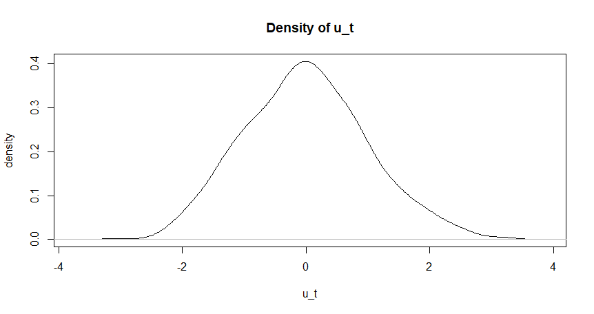
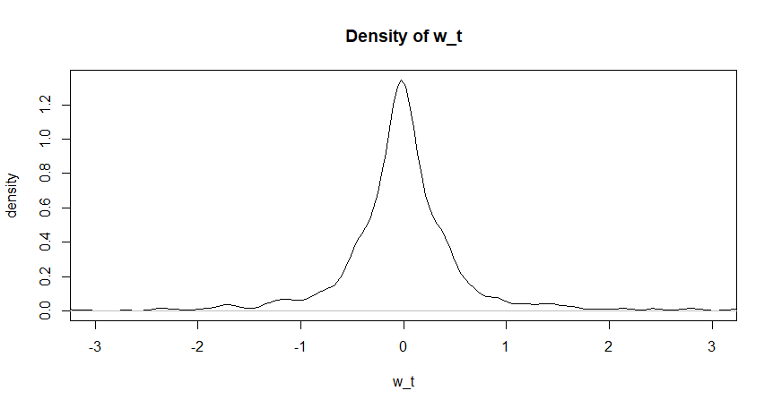
Figure 1: Estimated pdf of $u_{t}$ and $w_{t}$ based on the model residuals

Therefore, if we assume the error term of the return equation, $u_{t}$, is nonparametrically distributed and can be evaluated by kernel density estimation, then the approximation of posterior of volatility $h_{t}$ is

$$p(h_{t}|h_{t+1},h_{t-1},\delta,\alpha,\sigma_{\nu}^{2})\propto\frac{1}{h_{t}^{3/2}}\hat{f}\left(\frac{y_{t}}{\sqrt{h_{t}}}\right)\exp\left(-\frac{(\ln h_{t}-\mu_{t})^{2}}{2\sigma^{2}}\right)$$ (10)

Therefore, under the assumption of $u_{t}\sim f$ and $\nu_{t}\sim N(0,1)$, the likelihood is Equation 10, we name this model as NSVM-1. Additionally, the kernel density estimation of the two residuals provides an approximation of the new posterior of volatility $h_{t}$ is

$$p(h_{t}|h_{t+1},h_{t-1},\delta,\alpha,\sigma_{\nu}^{2})\propto\frac{1}{h_{t}^{3/2}}\hat{f}\left(\frac{y_{t}}{\sqrt{h_{t}}}\right)\hat{g}\left(\frac{\ln h_{t}-\mu_{t}}{\sigma_{\nu}}\right)$$ (11)

Similarly, under the assumption of $u_{t}\sim f$ and $\nu_{t}\sim g$, the likelihood is Equation 11, we name this model as NSVM-2.

Here $\hat{f}(x)=\frac{1}{n\times b}\sum_{i=1}^{n}N(\frac{x-x_{i}}{b})$, is the kernel density estimation of $\frac{\hat{u_{t}}-\mathrm{mean}(\hat{u_{t}})}{\mathrm{sd}(\hat{u_{t}})}$ and $\hat{g}(x)=\frac{1}{n\times b}\sum_{i=1}^{n}N(\frac{x-x_{i}}{b})$ is the kernel density estimation of $\frac{\hat{w_{t}}-\mathrm{mean}(\hat{w_{t}})}{\mathrm{sd}(\hat{w_{t}})}$, where $b$ is the bandwidth and $N$ is the density function of standard normal distribution. In our implementation, we use the built-in density function in R to obtain the kernel density estimation of Equation 10 11, and the bandwidth $b$ is chosen optimally using a standard bandwidth selection method. Details about bandwidth selection is showed in Appendix.

2.3 Algorithm

As is often the case, the nonparametric assumption for residuals means that the posterior distribution of $h_{t}$ lacks a closed-form expression. Consequently, we need a numerical method to sample from this posterior distribution to estimate both volatility and model parameters. In this paper, we will utilize the Metropolis-Hastings (MH) algorithm by Hastings, (1970), Metropolis et al., (1953), Tierney, (1994), Tierney, (1998) to address the challenge posed by intractable posterior distributions. This approach will also enable us to define customized proposal distributions for the specific model, enhancing the efficiency of the sampling process. Moreover, the MH algorithm demonstrates robust theoretical convergence by Rosenthal, (1995), Schmidler and Woodard, (2011), assuring reliable outcomes under mild assumptions, making it a strong candidate for posterior sampling.

Algorithm 1 presents a sketch of the primary algorithm. See Appendix: Algorithm 4 for a comprehensive discussion of the main sampler function.

Algorithm 1 Sketch main algorithm

$Input:(y,v_{0},s_{0},\delta_{0},\sigma_{\delta}^{2},\alpha_{0},\sigma_{\alpha}^{2},T,b)$

Initialize parameters $\delta$, $\alpha$, $\sigma_{\nu}$ and $h$

for i = 1,…,T+b do

  for t = 1,…,N-1 do

   Draw $h_{t}$ from its posterior distribution

  end for

  Let $h_{0}$ be the value such that $ln\ h_{1}=\alpha+\delta ln\ h_{0}+\sigma_{\nu}\nu_{1}$

  Let $ln\ h_{N}=\alpha+\delta ln\ h_{N-1}+\sigma_{\nu}\nu_{N}$

  Draw $\delta$ from its posterior distribution

  Draw $\alpha$ from its posterior distribution

  Draw $\sigma_{\nu}$ from its posterior distribution

end for

2.3.1 Semiparametric SVM algorithm with estimated pdf $f$

Nonparametric Bayesian methods offer considerable flexibility by allowing model complexity to grow with the data, adapting to the underlying structure without predefined assumptions about the number of parameters. This adaptability is particularly advantageous when the true structure of the data is unknown, as it enables the model to capture intricate patterns that parametric models may overlook.

If we relax the parametric normality assumption on $u_{t}$ and replace it with the kernel estimate of the pdf $f$ while maintaining the assumption that $\nu_{t}$ follows a standard normal distribution, this alteration will not influence the conditional posterior distributions of the parameters $\delta$, $\alpha$, and $\sigma_{\nu}$, based on the parametric prior proposed by Doan et al., (1994), i.e., $\alpha\sim N(\alpha_{0},\sigma_{\alpha}^{2})$, $\delta\sim N(\delta_{0},\sigma_{\delta}^{2})$, $\sigma_{\nu}^{2}\sim IG(\frac{\nu_{0}}{2},\frac{s_{0}}{2})$. Given the parametric form of these priors, sampling from these distributions remains straightforward.

The sampling approach introduced by Doan et al., (1994) provides an efficient mechanism for enhancing the updating step in the Metropolis-Hastings (MH) algorithm by Hastings, (1970), Tierney, (1994). This improvement hinges on an informed approximation of a specific distribution achieved through an inverse gamma distribution. The motivation for this selection is to match the first and second moments of the proposed distribution with those of the log-normal component in the posterior distribution. This alignment is established by calibrating the parameters of the inverse gamma distribution as follows:

The proposal distribution $q(h_{t})$ is defined by the equation:

$$q(h_{t})=\frac{\lambda^{\phi}}{\Gamma(\phi)}h^{-(\phi+1)}e^{-\frac{\lambda}{h_{t}}}$$ (12)

where $\lambda=\frac{1-2e^{\sigma^{2}}}{1-e^{\sigma^{2}}}+\frac{1}{2}$ and $\phi=(\lambda-1)e^{\mu_{t}+\frac{\sigma^{2}}{2}}+\frac{y_{t}^{2}}{2}$ are the parameters of inverse gamma distribution.

The sketch algorithm for sampling the volatility is shown in Algorithm 2.

Algorithm 2 Sketch algorithm of sampler for $h$

$Input:(y,\alpha,\delta,\sigma_{\nu}^{2},ln\_h_{i-1},h_{i},ln\_h_{i+1})$

Calculate $\mu$, $\sigma^{2}$, $\lambda$, $\phi$ by using input values

while not accepted do

  Draw the proposed $h_{new}\sim IG\left(\lambda,\phi\right)$

  Accept $h_{new}$ with probability $Min\left(1,\frac{p(h_{new})}{cq(h_{new})}\right)$, where $q$ is the density of inverse gamma distribution.

end while

if $p(h_{new})<cq(h_{new})$ then

  Return $h_{new}$

end if

Accept $h_{new}$ with probability $Min\left(1,\frac{p(h_{new})/q(h_{new})}{p(h_{old})/q(h_{old})}\right)$, where $h_{old}$ is previous sample of $h_{t}$

if accepted then

  Return $h_{new}$

else

  Return $h_{old}$

end if

Here the constant $c$ is defined as:

$$c=c^{\star}\left(\frac{p(h_{m})}{q(h_{m})}\right)$$ (13)

where $h_{m}$ is the mode of $q$ and $c^{\star}$ here is a tuning parameter. This constant serves as a scaling factor, ensuring that the proposed distribution $q(h_{t})$ closely mirrors the target distribution $p(h)$ in terms of its mode. In our implementation in the simulation, we choose $c^{\star}=1.2$, where by comparison of results in terms of bias, details about tuning $c^{\star}$ are shown in the Appendix. This nuanced calibration enhances the accuracy of the approximation and contributes to the overall efficiency and efficacy of the MH algorithm in navigating the complex landscape of the distribution under study. The detailed algorithm for sampling the volatility is included in Appendix: Algorithm 5.

2.3.2 Semiparametric SVM with independent unknown error distributions

In a real-world setting, the distribution of the error term in the return equation and the error term in the volatility equation are both unknown. Therefore, we utilize the same methodology to estimate them from data. By allowing the model’s complexity to evolve with real-world data, nonparametric Bayesian models provide more accurate uncertainty quantification.

If we assume the distributions of both error terms $u_{t}$ and $\nu_{t}$ are unknown, then nonparametric estimates of the joint distribution of fitted residuals $\hat{u_{t}}$ and $\hat{\nu_{t}}$ are needed. Consequently, the posterior distributions of $\delta$, $\alpha$, and $\sigma_{\nu}$ no longer have a parametric form. Therefore, numerical methods like MCMC must be utilized to sample from their nonparametric posterior distributions. Here, we use parameter $\delta$ as an example; similar sampling procedures are deployed on other parameters.

The sketch of the sampler algorithm for nonparametric $\delta$ is shown in Algorithm 3.

Algorithm 3 Sketch algorithm of sampler for $\delta$

$Input:(\delta_{0},\sigma_{\delta}^{2},\alpha,\sigma_{\nu}^{2},h,\delta_{left})$

Let proposal distribution $q$ be a normal distribution with the same mean and variance in the parametric setting

Let $p$ be the posterior distribution in the parametric setting

while not accepted do

  Draw proposed $\delta_{new}$ from proposal distribution

  Accept $\delta_{new}$ with probability $Min\left(1,\frac{p(\delta)}{q(\delta)}\right)$

end while

if $p(\delta)<q(\delta)$ then

  return $\delta_{new}$

end if

Accept $\delta_{new}$ with probability $Min\left(1,\frac{p(\delta_{new})/q(\delta_{new})}{p(\delta_{left})/q(\delta_{left})}\right)$, where $\delta_{left}$ is the previous sample of $\delta$

if accepted then

  return $\delta_{new}$

else

  return $\delta_{left}$

end if

The detailed algorithms for sampling posterior of parameters are included in Appendix: Algorithm 6, 7 and 8.

As mentioned in 11, the likelihood of volatility $h_{t}$ is also based on nonparametric estimates of the pdfs of the error terms $u_{t}$ and $\nu_{t}$. Thus, we utilize the same algorithm 2 but revise the posterior distribution of the volatility sequence $h_{t}$ from the equation 10 to equation 11.

3 Simulations and Application

This section examines the performance of the proposed method through simulations and an analysis of the S&P 500 data.

3.1 Simulation analysis

This section presents the results of applying our model to simulated data. In real-world scenarios, where the true values of volatility and the three parameters remain unknown, evaluating the performance differences between parametric and nonparametric models is quite challenging. In contrast, a generated simulation can offer a known ground truth for the estimated parameter values and realized volatility, enabling a more detailed comparison of model performance.

3.2 Simulation for Gaussian model

The objective here is to assess the performance of the proposed semiparametric method when the data-generating process involves normally distributed errors. In particular, we set $\alpha=-0.15$, $\delta=0.985$, $\sigma=0.15$.

Initialize $h_{0}\sim\mathrm{N}\left(\frac{\alpha}{1-\delta}=-10,\frac{\sigma}{\sqrt{1-\delta^{2}}}=0.87\right)$, $y_{0}\sim\sqrt{h_{0}}*\mathrm{N}\left(0,1\right)$. For $i=1,2,...,500$, $y_{i}=\sqrt{h_{i}}u_{i}$, $ln\left(h_{i}\right)=\alpha+\delta ln\left(h_{i-1}\right)+\sigma_{\nu}\nu_{i}$. Here $u_{i}\sim\mathrm{N}\left(0,1\right)$ and $\nu_{i}\sim\mathrm{N}\left(0,1\right)$. We run each MCMC for 10,000 iterations with the first 5,000 iterations designated as burn-in. Only the samples obtained after the 5,000-th iteration were retained for subsequent analysis.

To assess the precision and accuracy in parameter estimation, we repeated this process 100 times, each time we generated new $y_{1},...,y_{500}$ with the same parameter values and recorded the result: the mean, median, and mode of the posterior distributions, $p(\alpha|h,\delta,\sigma_{\nu}^{2})$, $p(\sigma_{\nu}^{2}|h,\alpha,\delta)$, and $p(\delta|h,\alpha,\sigma_{\nu}^{2})$. Figures 2, 3 and 4 present the results for the Gaussian, NSVM-1, and NSVM-2 models, respectively. The red dashed lines indicate the true values used in generating the data.

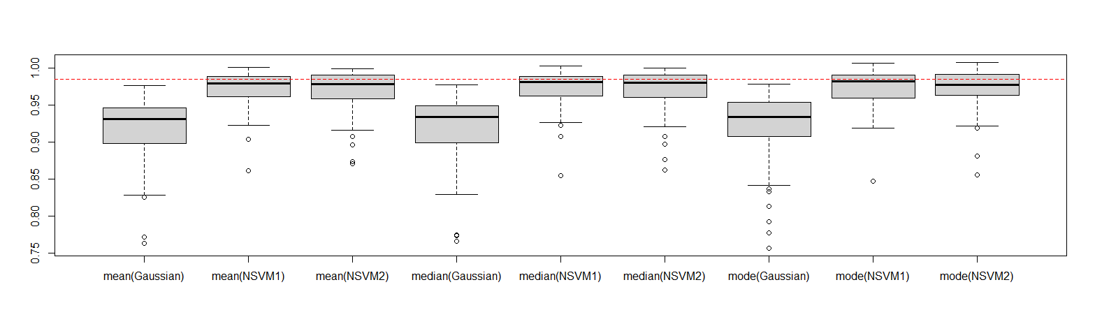
Figure 2: Estimation of delta under Gaussian error model simulation. The dotted line is the true value (0.985)

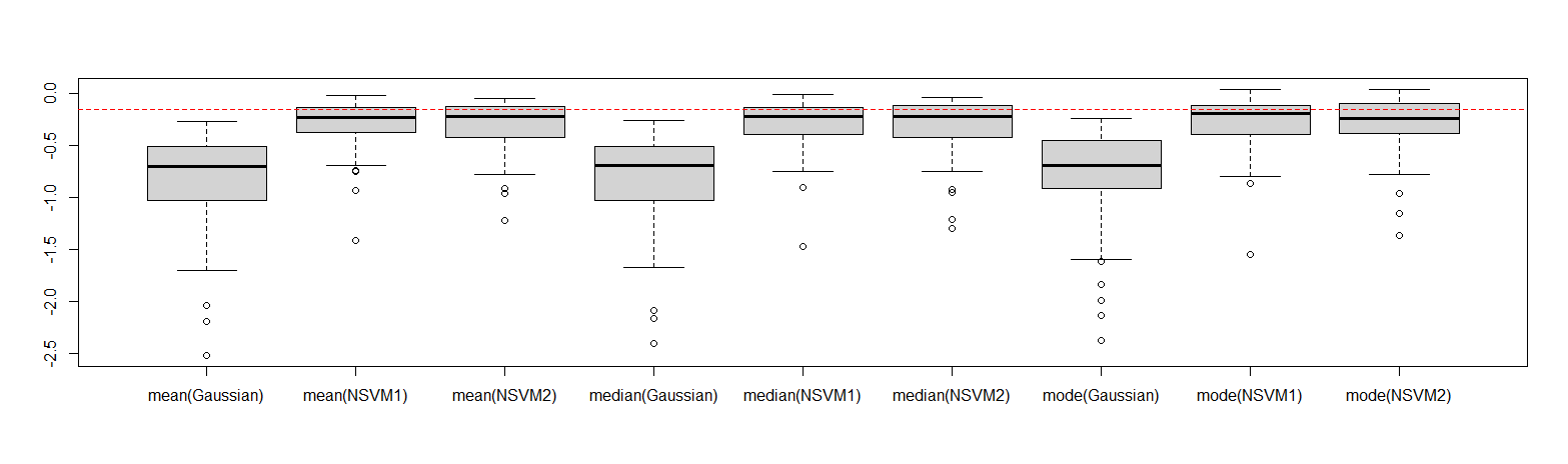
Figure 3: Estimation of delta under Gaussian error model simulation. The dotted line is the true value (-0.15)

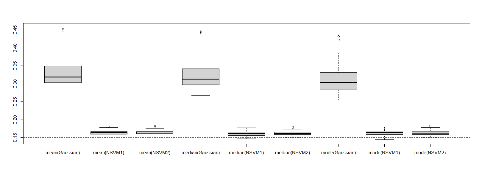
Figure 4: Estimation of sigma under Gaussian error model simulation. The dotted is the true value (0.15)

As shown in the box plots, the results from the NSVM-1 and NSVM-2 models exhibit a minor deviation from the red dashed line, representing the actual value than those of the Gaussian model, indicating lower bias. Furthermore, the narrower range of the box plots for NSVM-1 and NSVM-2 suggests a substantially lower variance of these estimates. Additionally, the plots reveal no significant differences among the distributions’ mean, median, or mode. To quantitatively assess performance, we define the mean square error (MSE) of them can be defined as $\frac{1}{100}\left(\Sigma\bar{\delta_{i}}-\delta\right)^{2}$, $\frac{1}{100}\left(\Sigma\bar{\alpha_{i}}-\alpha\right)^{2}$ and $\frac{1}{100}\left(\Sigma\bar{\sigma_{\nu i}}-\sigma_{\nu}\right)^{2}$. For the Gaussian model, the MSE of mean, median, and mode for $\delta$ are all approximately 0.004, whereas the MSEs for NSVM-1 and NSVM-2 are 0.000156 and 0.000213, respectively. For $\alpha$, the MSE for the Gaussian model is 0.4526, while for NSVM-1 and NSVM-2, it is 0.0297 and 0.0363, respectively. For $\sigma_{\nu}$, the Gaussian model yields an MSE of 0.0314, whereas the NSVM-1 and NSVM-2 models yield significantly lower MSE values of 0.000187 and 0.000183, respectively.

The results show that the proposed semiparametric methods outperform the traditional parametric SVM, even in the ideal setup where the data-generating process is Gaussian and the fitted model is correctly specified. This demonstrates that a parametric model cannot account for the anomalies in the data, while the semiparametric approaches offer a superior alternative by providing better accounting for the features of the data.

3.3 Simulations for heavy-tailed error distributions

Alongside simulations using normally distributed error settings, we assess the model’s performance with heavy-tailed error distributions, including the Student’s t distribution and the Generalized Error Distribution (GED). Analyzing heavy-tailed error distributions is essential since real-world data frequently display leptokurtic traits that diverge from the Gaussian norm. Models demonstrating strong performance under these distributions are more applicable in fields like finance and economics, where such distributions are prevalent, thereby enhancing the robustness and versatility of volatility estimation techniques. In the following discussion, we will maintain the same parameter values as in the prior section; the sole variation is in the error term distributions, $u_{i}$ and $u_{i}$.

3.3.1 Student’s t distributed error simulation

The Student’s t distribution, especially with low degrees of freedom, is recognized for its heavy tails, which increase the chances of extreme values compared to the normal distribution. The heaviness of the tails is influenced by the degrees of freedom; fewer degrees lead to heavier tails, allowing the distribution to approximate normality as the degrees of freedom rise Sundararajan and Barreto-Souza, (2021). In our simulation, we set $u_{i}$ and $u_{i}$ to follow a Student’s t distribution with 10 degrees of freedom. Figures 5, 6, and 7 show the results of the Student’s t distributed error simulation for the Gaussian, NSVM-1, and NSVM-2 models, respectively, with the red dashed lines indicating the true values used to generate the data.

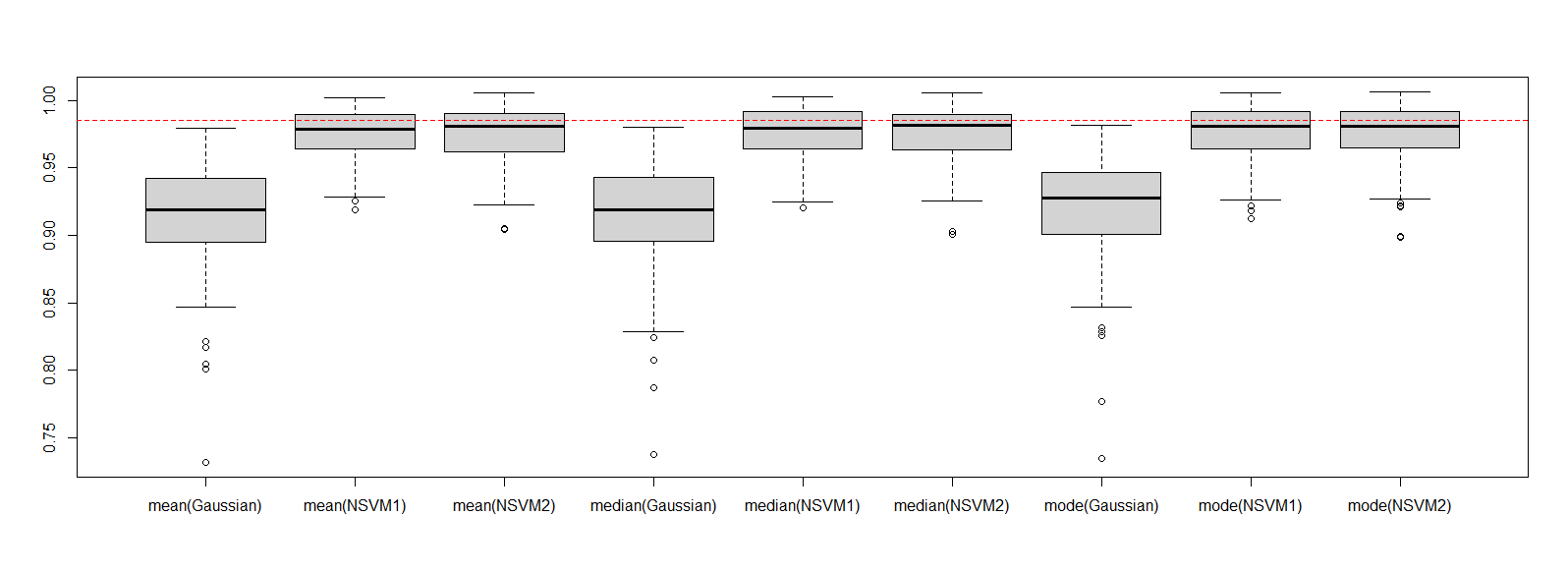
Figure 5: Estimation of delta under Student’s t-distribution error model simulation. The dotted line is the true value (0.985)

Figure 6: Estimation of alpha under Student’s t-distribution error model simulation. The dotted line is the true value (-0.15)

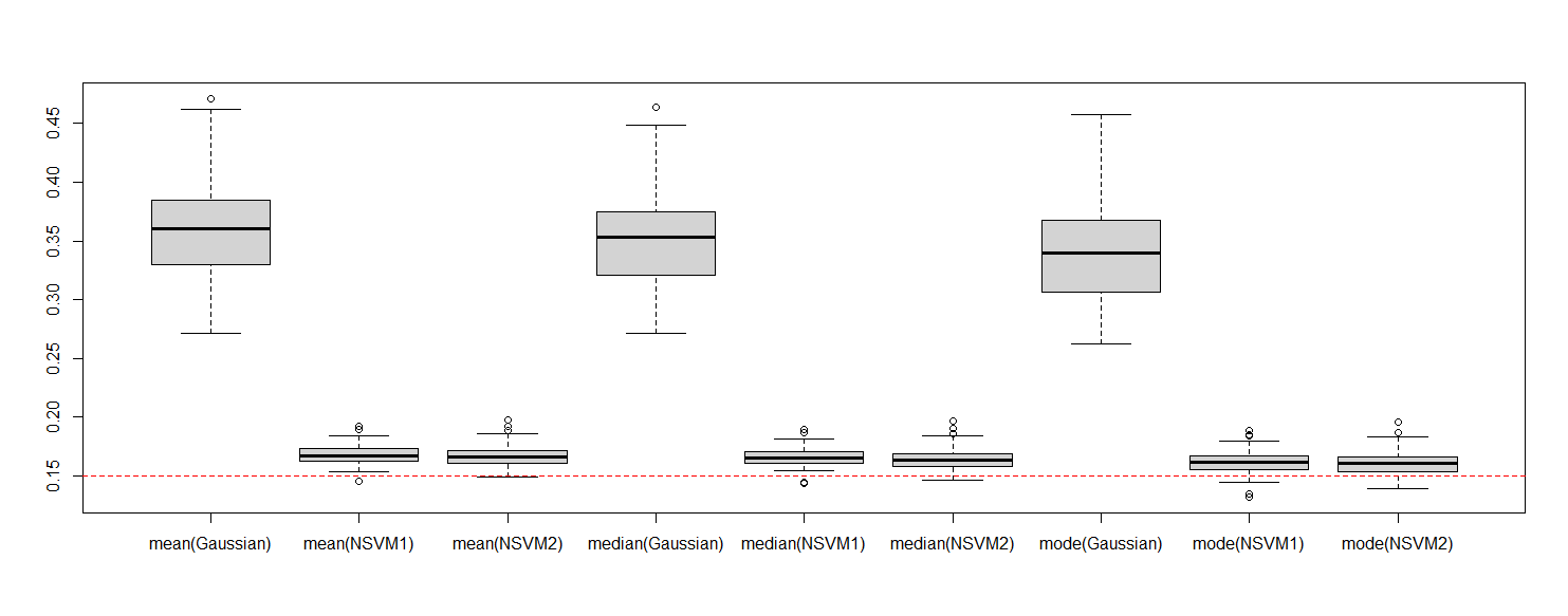
Figure 7: Estimation of sigma under Student’s t-distribution error model simulation. The dotted line is the true value (0.15)

In line with the findings from the Gaussian simulation, the NSVM-1 and NSVM-2 models exhibit a smaller deviation from the red dashed line, which denotes the true parameter value, compared to the Gaussian model, thus indicating a reduction in bias. Furthermore, the box plots for NSVM-1 and NSVM-2 present a narrower range, signifying considerably less variance in these estimates. The plots show no significant differences regardless of whether the mean, median, or mode is used to assess central tendency. For the Gaussian model, the mean squared error (MSE) for the mean, median, and mode of $\delta$ is about 0.005, while the MSEs for NSVM-1 and NSVM-2 are 0.0001008 and 0.0001076, respectively. In terms of $\alpha$, the MSE for the Gaussian model stands at 0.5431, in contrast to 0.024 for NSVM-1 and 0.025 for NSVM-2. For $\sigma_{\nu}$, the Gaussian model yields an MSE of 0.04408, while NSVM-1 and NSVM-2 deliver significantly lower MSE values of 0.00031 and 0.00028, respectively.

3.3.2 Simulations based on GED error

The Generalized Error Distribution (GED) is a continuous probability distribution defined by its adaptable tail thickness, offering enhanced flexibility in modeling heavy-tailed data Catania, (2022). In contrast to the normal distribution, the GED features a shape parameter that regulates the kurtosis. As this parameter diminishes, the tails grow heavier, making it appropriate for datasets with frequent large deviations from the mean. This distribution is frequently utilized in financial modeling and various domains where extreme values and outliers are common. In the simulation setup, we define $u_{i}$ and $\nu_{i}$ to adhere to a GED distribution characterized by a mean of 0 and a variance of 1. The results from the GED-distributed error simulation for the Gaussian, NSVM-1, and NSVM-2 models are shown in Figures 8, 9, and 10, respectively. As previously mentioned, the red dashed lines indicate the true values utilized for data generation.

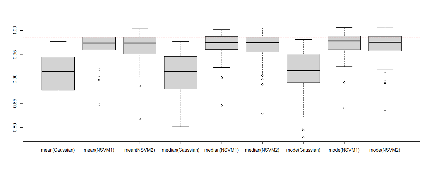
Figure 8: Estimation of delta under GED error model simulation. The dotted line is the true value (0.985)

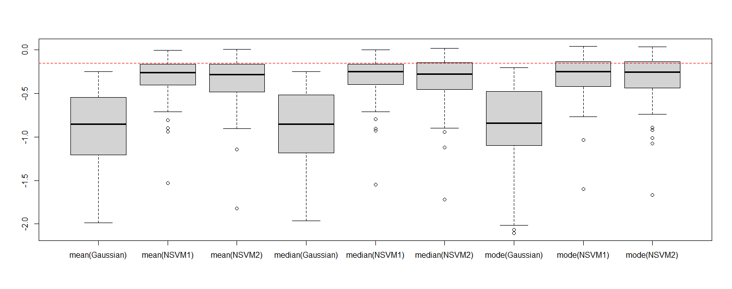
Figure 9: Estimation of alpha under GED error model simulation. The dotted line is the true value (-0.15)

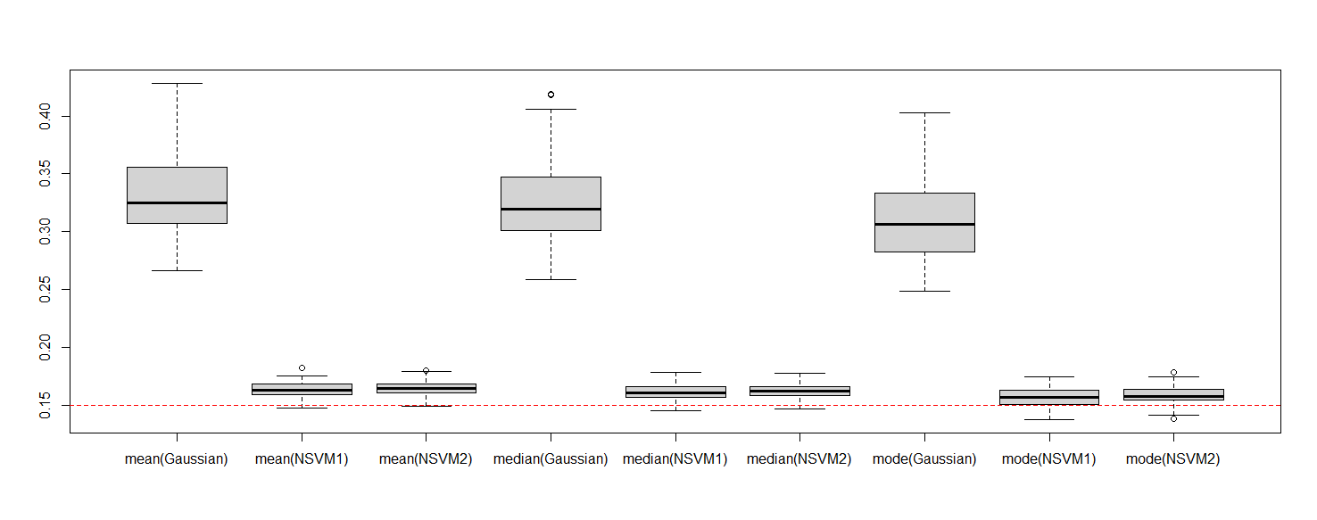
Figure 10: Estimation of sigma under GED error model simulation. The dotted line is the true value (0.15)

The plot reveals steady trends, indicating that the NSVM-1 and NSVM-2 models perform better than the Gaussian model in terms of bias and variance. This is clear from the mean squared error (MSE) comparisons among all three models. For the parameter $\delta$, the Gaussian model reports MSE values around 0.0058 for the mean, median, and mode, reflecting a greater bias and variability in these estimates. In comparison, the NSVM-1 and NSVM-2 models demonstrate significantly lower MSE values of 0.00023 and 0.00035, respectively, highlighting their enhanced precision in parameter estimation.

For $\alpha$, the Gaussian model shows a notably higher MSE of 0.6663, signifying substantial estimation errors. In contrast, the NSVM-1 and NSVM-2 models achieve significantly lower MSE values of 0.0458 and 0.0616, respectively, suggesting these models are better at accurately capturing the true parameter values while reducing errors.

For $\sigma_{\nu}$, performance differences stand out clearly. The Gaussian model yields a mean squared error (MSE) of 0.03348, significantly surpassing the lower MSE values of NSVM-1 and NSVM-2 at 0.000175 and 0.000211, respectively. This evidence highlights the superior ability of NSVM-1 and NSVM-2 to deliver more accurate and reliable estimates, particularly in capturing nuanced variations while ensuring robustness in parameter estimation. This overall enhancement in performance illustrates the benefits of the NSVM frameworks compared to traditional Gaussian modeling methods.

3.4 Volatility Estimation

To assess the model’s effectiveness in estimating volatility, we create a dataset using the same parameters as outlined earlier: $\alpha=-0.10$, $\delta=0.985$, $\sigma=0.15$. The algorithm is run with the identical data input for 100 repetitions. Each run involves executing the MCMC algorithm for 10,000 iterations, with 5,000 iterations considered as burn-in, hence keeping only the latter half of the samples. We collect the final 5,000 sampled volatility values from the posterior distribution. After the simulation concludes, we calculate the mean of these recorded volatility samples to provide the estimated volatility. This method utilizes Gaussian error simulation, and the estimated volatility from the Gaussian model, as well as NSVM-1 and NSVM-2 models, is illustrated in Figure 11.

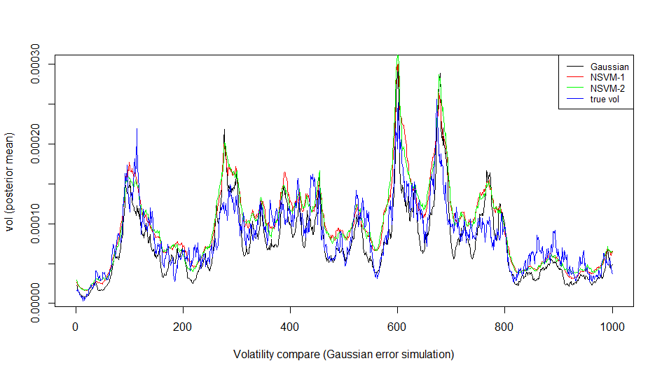
Figure 11: Comparison of volatility for Gaussian error simulation)

For Student-t error simulation, the comparison is shown in Figure 12.

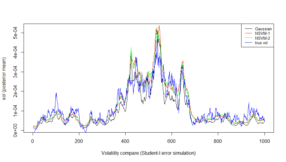
Figure 12: Comparison of volatility for Student’s t-distribution error simulation)

For GED error simulation, the comparison is shown in Figure 13.

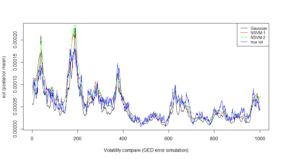
Figure 13: Comparison of volatility for GED error simulation)

Figures 11, 12, and 13 show that the NSVM-1 and NSVM-2 models outperform the traditional Gaussian model in estimating volatility. For example, in Figure 12, at around $t=500$ and $t=600$, the Gaussian model’s volatility estimates are significantly lower than the actual values, while NSVM-1 and NSVM-2 provide estimates that closely match the true volatility. A consistent trend can be seen in Figure 13, especially near $t=220$ and $t=380$, where NSVM-1 and NSVM-2 accurately capture the true volatility, unlike the Gaussian model, which falls short.

This discrepancy arises from the Gaussian model’s assumption about the error term, which does not account for the heavy-tailed distribution utilized in the simulation. On the other hand, the NSVM-1 and NSVM-2 models are more appropriate for situations with heavy-tailed errors, showcasing their resilience and flexibility. These findings underscore the benefits of employing NSVM frameworks, whether dealing with heavy-tailed error distributions or when the error distribution is Gaussian and the parametric model is accurately defined.

Additionally, we use the following metrics to assess and compare volatility estimation performance. Let the actual volatility from the simulation be represented as $h_{1},...,h_{N}$, and the estimated volatility as $\bar{h_{1}},...,\bar{h_{N}}$. Besides the mean, we also take into account the median and mode of the final sampled volatilities for comparison. The three metrics used to assess volatility estimation performance are: square root of mean square error (srMSE), $\sqrt{\frac{\Sigma(h_{i}-\bar{h_{i}})^{2}}{N}}$, mean absolute error (MAE), $\frac{\Sigma|h_{i}-\bar{h_{i}}|}{N}$, and mean absolute percent error (MAPE), $\frac{1}{N}\Sigma\frac{|h_{i}-\bar{h_{i}}|}{h_{i}}\times 100\%$. The table 1 presents the results of Gaussian error simulation. Table 2 displays the outcomes of the Student’s t error simulation, while Table 3 presents the results of the GED error simulation.

Model	srMSE Mean	srMSE Median	srMSE Mode	MAE Mean	MAE Median	MAE Mode	MAPE Mean	MAPE Median	MAPE Mode
Gaussian	0.008278	0.008287	0.008296	0.007433	0.007341	0.007347	0.09932	0.09908	0.09922
NSVM-1	0.008252	0.008260	0.008271	0.007313	0.007325	0.007327	0.09945	0.09927	0.09912
NSVM-2	0.008250	0.008259	0.008269	0.007213	0.007318	0.007314	0.09959	0.09939	0.09944

Table 1: Volatility estimation error comparison (Gaussian error simulation)

Model	srMSE Mean	srMSE Median	srMSE Mode	MAE Mean	MAE Median	MAE Mode	MAPE Mean	MAPE Median	MAPE Mode
Gaussian	0.006675	0.006682	0.006691	0.006019	0.006025	0.006031	0.09959	0.09968	0.09977
NSVM-1	0.006648	0.006656	0.006677	0.005997	0.006005	0.006011	0.09948	0.09957	0.09965
NSVM-2	0.006651	0.006651	0.006668	0.005998	0.006003	0.006009	0.09949	0.09959	0.09966

Table 2: Volatility estimation error comparison (Student-t error simulation)

Model	srMSE Mean	srMSE Median	srMSE Mode	MAE Mean	MAE Median	MAE Mode	MAPE Mean	MAPE Median	MAPE Mode
Gaussian	0.006408	0.006411	0.006416	0.005947	0.005951	0.005955	0.09967	0.09973	0.09979
NSVM-1	0.006395	0.006398	0.006404	0.005935	0.005938	0.005943	0.09964	0.09969	0.09973
NSVM-2	0.006394	0.006396	0.006403	0.005934	0.005939	0.005939	0.09966	0.09971	0.09977

Table 3: Volatility estimation error comparison (GED error simulation)

The tables 1, 2, and 3 illustrate that the volatilities estimated by the NSVM-1 and NSVM-2 models show lower square root mean squared error (srMSE), mean absolute error (MAE) and mean absolute percentage error (MAPE). This trend holds true except for the MAPE derived from the mean and median of the final sampled volatilities for the Gaussian error simulation. These reduced levels of bias offer assurance that NSVM-1 and NSVM-2 offer enhanced accuracy in estimating volatility.

3.5 Empirical application

This section presents the results from using our model on daily stock return data. The S$\&$P 500 (Standard and Poor’s 500) is a stock market index that measures the performance of 500 of the largest publicly traded companies in the U.S. It is considered one of the best indicators of the U.S. stock market’s overall performance and the economy at large. Here, we analyze the daily closing price of the S$\&$P 500 from February 1, 2021, to February 1, 2024. The simulation section demonstrates that the model also provides sampled volatility and estimated parameter values. We employed the Gaussian model, NSVM-1, and NSVM-2, using the log return of the closing price ($\log\left(Price_{t}/Price_{t-1}\right)$) as input. Each of the three models was executed 100 times, running MCMC for 10,000 iterations with 5,000 burn-ins; this means we only retained samples after the 5,000th iteration. For volatility estimation, we captured the last sample from the 5,000 sampled values of the volatility time series from the posterior distribution.

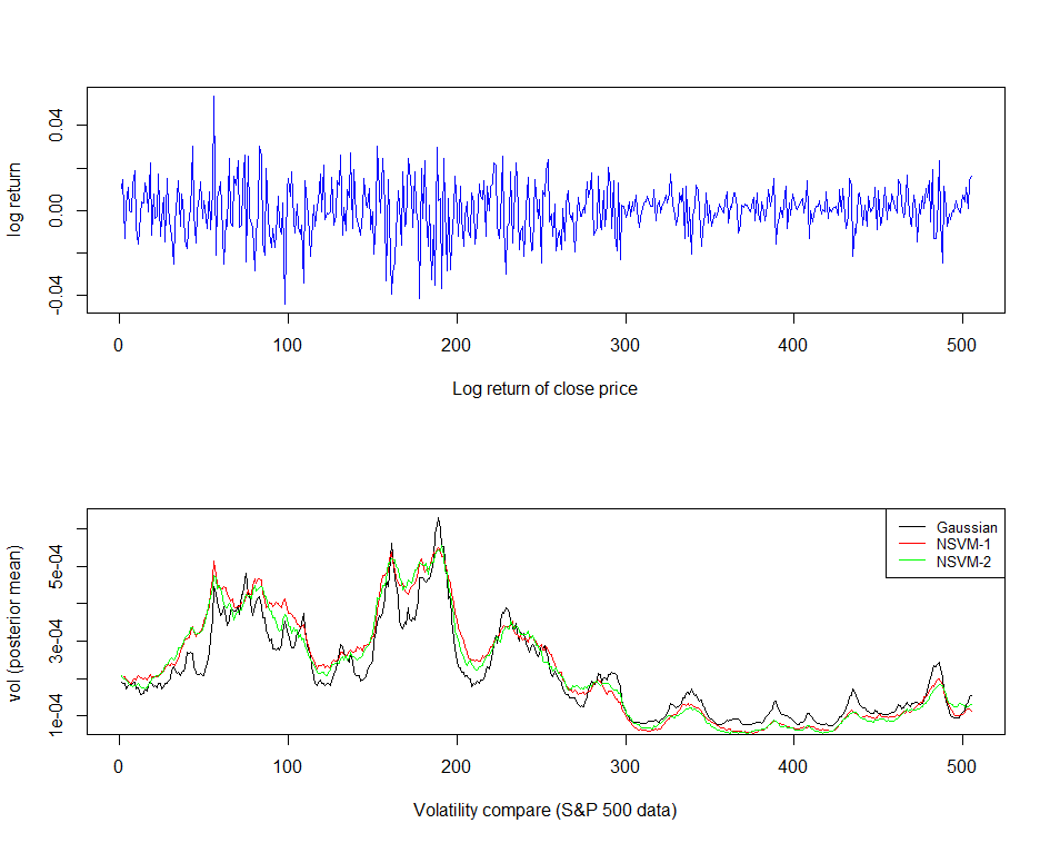
Figure 14: Comparison of volatility estimates of S$\&$P 500 series

The upper plot in Figure 14 illustrates the logarithm of the return on the closing price for that period, while the lower plot displays the average recorded volatility derived from the Gaussian model, NSVM-1 model, and NSVM-2 model. Notably, the estimated volatility shows a significant rise at points such as $t=60$ and $t=190$, reacting to considerable fluctuations in return values, whether these represent gains or losses. This pattern highlights that the estimated volatility effectively reflects the degree of price movements, indicating the strength of these changes.

For parameter estimation, we record the means of the posterior distributions, $p(\alpha|h,\delta,\sigma_{\nu}^{2})$, $p(\sigma_{\nu}^{2}|h,\alpha,\delta)$, and $p(\delta|h,\alpha,\sigma_{\nu}^{2})$. Figure 15 displays the box plots of the means based on 100 repetitions of parameter estimates.

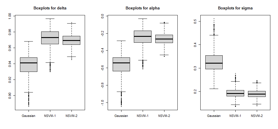
Figure 15: Box-plots of parameter estimates of the SV model, S$\&$P 500 data

In real-world situations, determining the true values of parameters can be quite difficult, unlike simulations where these values are pre-set and easily accessible. This difficulty arises from the intricate nature of actual data, which is frequently affected by a variety of non-financial factors.

4 Conclusions

This paper presents a semiparametric method for modeling stochastic volatility (SV). It employs nonparametric estimation for the error distribution to address the limitations of Gaussian assumptions in traditional parametric models. By integrating this nonparametric framework into a Bayesian Markov Chain Monte Carlo (MCMC) approach, we aim to better capture the non-Gaussian features commonly observed in financial return data, enhancing the model’s flexibility and accuracy.

Our extensive simulation findings highlight the benefits of the non-parametric SV models (NSVM-1 and NSVM-2) compared to traditional Gaussian models, especially in the presence of heavy-tailed errors. These non-parametric models consistently exhibit lower bias and variance when evaluated using simulated data across Gaussian, Student-t, and Generalized Error Distributions (GED). Key performance indicators, including the root mean squared error (srMSE), mean absolute error (MAE) and mean absolute percentage error (MAPE), demonstrate that non-parametric models surpass parametric alternatives in all scenarios, with notable improvements in heavy-tailed distributions. These findings suggest that non-parametric models excel in adjusting to non-Gaussian error patterns, resulting in more precise estimates of volatility and parameters.

The empirical examination of S$\&$P 500 data illustrates its practical significance and aligns well with actual volatility measures, like the VIX index. Nevertheless, the key contribution of this study lies in demonstrating the effectiveness of the proposed semiparametric methods through controlled simulations. The findings validate that the NSVM-1 and NSVM-2 models provide a more nuanced representation of financial volatility dynamics, enhancing the precision of risk assessments.

This paper introduces a novel method for modeling volatility by integrating a semiparametric framework into the SV model. However, the findings have some limitations. Specifically, the model assumes that the error distributions, $u_{t}$ and $\nu_{t}$, are independent, which may not reflect reality. Future research could seek to relax this assumption by examining the joint distribution of the error terms and adjusting the likelihood accordingly. Another promising direction is to improve kernel density estimation techniques in this framework, potentially by incorporating dynamic bandwidth selection to better handle time-varying volatility. Additionally, applying this non-parametric approach to multivariate financial models may enhance adaptability and accuracy in capturing intricate financial behaviors across diverse datasets.

5 Appendix

5.1 Effect of sample size in simulation

We utilized the algorithm with a time series of 500 length and also evaluated it with lengths of 2000 and 5000. These simulations incorporated errors based on Normal, Student’s t, and GED distributions. This approach enabled us to evaluate outcomes across different data lengths and assess the algorithm’s performance in various contexts.

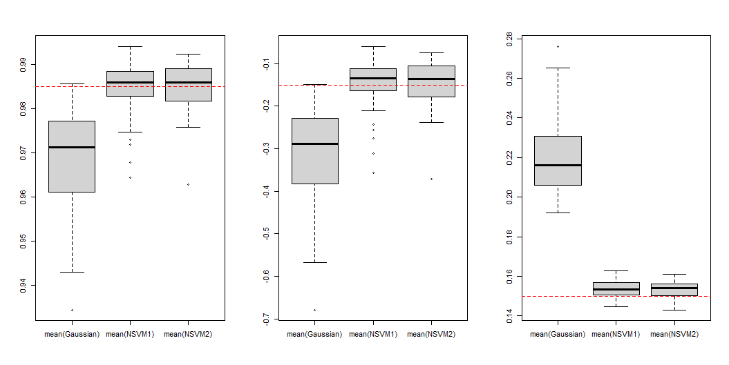
Figure 16: Box-plots of parameter estimates of Gaussian error model, sample size 2000.

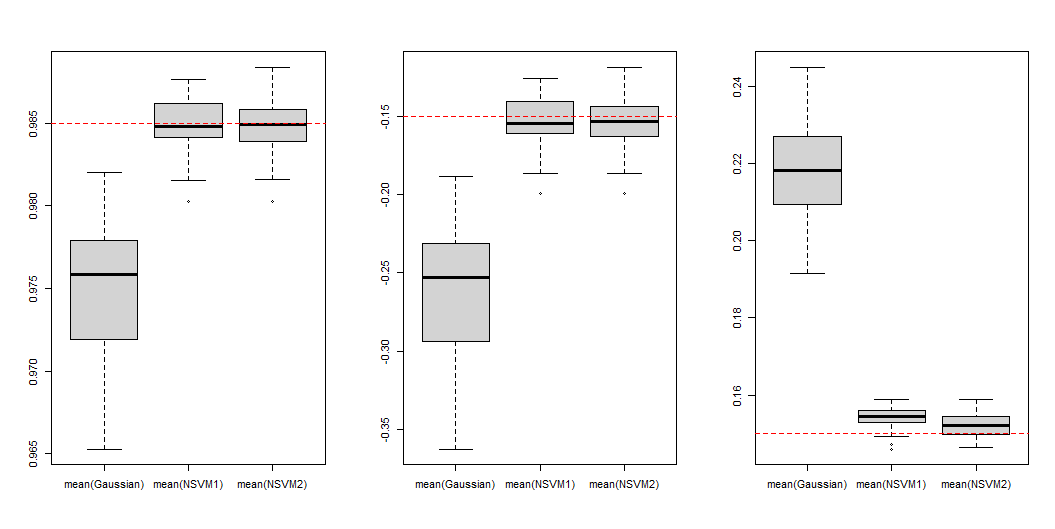
Figure 17: Box-plots of parameter estimates of Student’s t error model, sample size 2000.

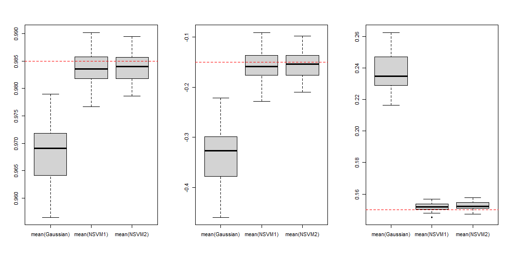
Figure 18: Box-plots of parameter estimates of the GED error model, sample size 2000.

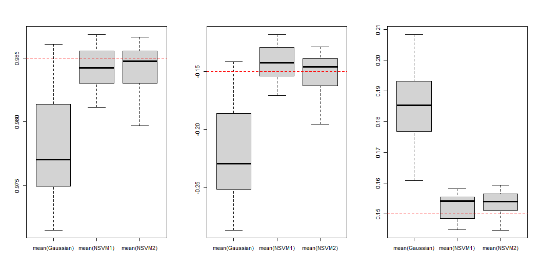
Figure 19: Box-plots of parameter estimates of Gaussian error model, sample size of 5000.

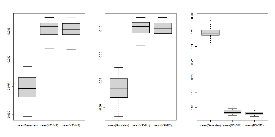
Figure 20: Box-plots of parameter estimates of Student’s t error model, sample size 5000.

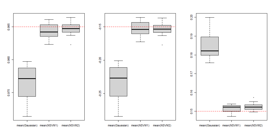
Figure 21: Box-plots of parameter estimates of the GED error model, sample size 5000.

5.2 Tuning parameters and bandwidth

Tuning parameters plays a vital role in performance, ensuring a proper balance between exploration and convergence. The tuning parameter $c^{\star}$ illustrated in equation 13 must be adjusted with care to achieve optimal outcomes. This adjustment is crucial because an incorrectly set parameter can result in elevated rejection rates and ineffective sampling. We implement a grid search for parameter tuning, adjusting $c^{\star}$ in increments of 0.1 from 0.8 to 1.4. For each value, we fit the model and record the mean of the posterior for the parameter, repeating this process 50 times. Consequently, we have $\bar{\delta_{i}}$, $\bar{\alpha_{i}}$ and $\bar{\sigma_{\nu i}}$ for $i=1,2,...,50$, and the mean square error (MSE) can be defined as $\frac{1}{50}\left(\Sigma\bar{\delta_{i}}-\delta\right)^{2}$, $\frac{1}{50}\left(\Sigma\bar{\alpha_{i}}-\alpha\right)^{2}$ and $\frac{1}{50}\left(\Sigma\bar{\sigma_{\nu i}}-\sigma_{\nu}\right)^{2}$. The results are presented in Table 4 and Table 5. We select $c^{\star}=1.2$ for simulations because this choice minimizes the mean squared errors in the estimation of parameters.

Value of $c^{\star}$		0.8	0.9	1.0	1.1
MSE of $\delta$	Gaussian	$2.567*10^{-4}$	$2.459*10^{-4}$	$1.831*10^{-4}$	$1.263*10^{-4}$
	NSVM-1	$2.131*10^{-4}$	$1.983*10^{-4}$	$1.211*10^{-4}$	$1.067*10^{-4}$
	NSVM-2	$1.862*10^{-4}$	$1.438*10^{-4}$	$1.181*10^{-4}$	$8.856*10^{-5}$
MSE of $\alpha$	Gaussian	0.0234	0.0261	0.0184	0.0139
	NSVM-1	0.0396	0.0376	0.0361	0.0139
	NSVM-2	0.0385	0.0298	0.0236	0.0113
MSE of $\sigma_{\nu}$	Gaussian	$1.423*10^{-4}$	$1.127*10^{-4}$	$5.532*10^{-5}$	$7.473*10^{-5}$
	NSVM-1	$1.123*10^{-4}$	$1.142*10^{-4}$	$7.351*10^{-5}$	$1.263*10^{-4}$
	NSVM-2	$2.567*10^{-4}$	$2.459*10^{-4}$	$1.831*10^{-4}$	$9.236*10^{-5}$

Table 4: Table of MSE of parameter estimates by different $c^{\star}$

Value of $c^{\star}$		1.2	1.3	1.4
MSE of $\delta$	Gaussian	$9.542*10^{-5}$	$1.434*10^{-4}$	$1.231*10^{-4}$
	NSVM-1	$1.051*10^{-4}$	$1.893*10^{-4}$	$2.231*10^{-4}$
	NSVM-2	$9.943*10^{-5}$	$1.435*10^{-4}$	$1.641*10^{-4}$
MSE of $\alpha$	Gaussian	0.0164	0.0174	0.0189
	NSVM-1	0.0135	0.0194	0.0219
	NSVM-2	0.0125	0.0147	0.0253
MSE of $\sigma_{\nu}$	Gaussian	$9.348*10^{-5}$	$1.542*10^{-4}$	$1.135*10^{-4}$
	NSVM-1	$9.542*10^{-5}$	$1.434*10^{-4}$	$1.231*10^{-4}$
	NSVM-2	$9.853*10^{-5}$	$1.141*10^{-4}$	$1.096*10^{-4}$

Table 5: Table of MSE of parameter estimates by different $c^{\star}$ (cont.)

Selecting the right bandwidth is critical in kernel density estimation; the bandwidth parameter $b$ influences the smoothness of the density estimate by defining the width of the kernel function. In our implementation, we assessed various built-in methods for bandwidth selection available in R, including nrd0 Silverman, (1986), bcv Scott and Terrell, (1987), and SJ Sheather and Jones, (2018). The results show no noteworthy performance variations among the different bandwidth selection options. As a result, the algorithm adopted the default bandwidth method. nrd0, in R.

5.3 Detailed algorithms

This section provides a detailed description of the algorithms discussed in the paper.

$Input:(y,v_{0},s_{0},\delta_{0},\sigma_{\delta}^{2},\alpha_{0},\sigma_{\alpha}^{2},T,b)$

$N\leftarrow length(y)$

$\delta\leftarrow 1$

$\alpha\leftarrow 0$

$\sigma_{\nu}^{2}\leftarrow 0.1$

$h\leftarrow rep(var(y),N)$

$ln\_h\leftarrow log(h)$

$h\_sample\leftarrow matrix(N,T)$

$\delta\_sample\leftarrow rep(0,T)$

$\alpha\_sample\leftarrow rep(0,T)$

$\sigma_{\nu}^{2}\_sample\leftarrow rep(0,T)$

for $ite\ in\ 1\ to\ (T+b)$ do

  for $i\ in\ 2\ to\ N-1$ do

   $r\leftarrow sample\_h(y[i],\alpha,\delta,\sigma_{\nu}^{2},ln\_h[i-1],ln\_h[i+1])$

   $h[i]\leftarrow r\$h\_new$

   $ln\_h\leftarrow log(h[i])$

  end for

  $ln\_h[1]\leftarrow rnorm(1,\alpha+\delta*ln\_h[2],\sqrt{\sigma_{\nu}^{2}})$

  $ln\_h[N]\leftarrow rnorm(1,\alpha+\delta*ln\_h[N-1],\sqrt{\sigma_{\nu}^{2}})$

  $h[1]\leftarrow exp(ln\_h[1])$

  $h[N]\leftarrow exp(ln\_h[N])$

  $s_{1}\leftarrow sum(ln\_h)$

  $s_{2}\leftarrow sum(ln\_h^{2})$

  $s_{3}\leftarrow sum(ln\_h[1:(N-1)]*ln\_h[2:N])$

  $s^{\prime}\leftarrow s_{0}+(N-1)\alpha^{2}+(1+\delta^{2})s_{2}-\delta^{2}(ln\_h[N])^{2}-ln\_h[1]^{2}-2\alpha((1-\delta)s_{1}-ln\_h[1]+\delta ln\_h[N])-2\delta s_{3}$

  $\sigma_{\nu}^{2}\leftarrow sample\_\sigma_{\nu}^{2}(v_{0},s^{\prime},\alpha,\delta,h,\sigma_{\nu}^{2}\_sample[ite-1])$

  $\alpha\leftarrow sample\_\alpha(\alpha_{0},\sigma_{\alpha}^{2},\delta,\sigma_{\nu}^{2},h,\alpha\_sample[ite-1])$

  $\delta\leftarrow sample\_\delta(\delta_{0},\sigma_{\delta}^{2},\alpha,\sigma_{\nu}^{2},h,\delta\_sample[ite-1])$

  if $ite>b$ then

   $\alpha\_sample[ite-b]\leftarrow\alpha$

   $\delta\_sample[ite-b]\leftarrow\delta$

   $\sigma_{\nu}^{2}\_sample[ite-b]\leftarrow\sigma_{\nu}^{2}$

   $h\_sample[ite-b]\leftarrow h$

  end if

end for

return $(h\_sample,\alpha\_sample,\delta\_sample,\sigma_{\nu}^{2}\_sample)$

Algorithm 4 Main

$Input:(y,\alpha,\delta,\sigma_{\nu}^{2},ln\_h_{i-1},ln\_h_{i+1})$

$\mu\leftarrow\frac{\delta(ln\_h_{i-1}+ln\_h_{i+1})+(1+\delta)\alpha}{1+\delta^{2}}$

$\sigma^{2}\leftarrow\frac{\sigma_{\nu}^{2}}{1+\delta^{2}}$

$\lambda\leftarrow\frac{1-2exp(\sigma^{2})}{1-exp(\sigma^{2})}+0.5$

$\phi\leftarrow(\lambda-1)exp(\mu+\frac{\sigma^{2}}{2})+\frac{y^{2}}{2}$

$qmode=\frac{\phi}{1+\lambda}$

$ln\_c\leftarrow ln(1.2)+ln\_p(y,qmode,\alpha,\delta,\sigma_{\nu}^{2})-ln(dinvgamma(qmode,\lambda,\phi))$

$h\_new\leftarrow rinvgamma(1,\lambda,\phi)$

$threshold_{1}\leftarrow\frac{exp(ln\_p(y,h\_new,qmode,\alpha,\delta,\sigma_{\nu}^{2})-ln\_c)}{dinvgamma(h\_new,\lambda,\phi)}$

$roll\leftarrow runif(1)$

while $roll>threshold_{1}$ do

  $h\_new\leftarrow rinvgamma(1,\lambda,\phi)$

  $threshold_{1}\leftarrow\frac{exp(ln\_p(y,h\_new,qmode,\alpha,\delta,\sigma_{\nu}^{2})-ln\_c)}{dinvgamma(h\_new,\lambda,\phi)}$

  $roll\leftarrow runif(1)$

end while

if $threshold_{1}\geq 1$ then

  $threshold_{2}\leftarrow exp(ln\_p(y,h\_new,qmode,\alpha,\delta,\sigma_{\nu}^{2})-ln\_p(y,h,qmode,\alpha,\delta,\sigma_{\nu}^{2})+log(dinvgamma(h,\lambda,\phi))-log(dinvgamma(h\_new,\lambda,\phi)))$

  $roll\leftarrow runif(1)$

  if $roll>threshold_{2}$ then

   $h\_new\leftarrow h$

  end if

end if

return $h\_new$

Algorithm 5 Sampler for $h$

$Input:(v_{0},s^{\prime},\alpha,\delta,h,\sigma^{2}_{left})$

$q(\sigma_{\nu}^{2})\sim IG(\frac{v_{0}+N-1}{2},\frac{s^{\prime}}{2})$

$p(\sigma_{\nu}^{2})\leftarrow p(\sigma_{\nu}^{2}|h,\alpha,\delta)$

$c\leftarrow\frac{p(\sigma_{\nu}^{2})}{q(\sigma_{\nu}^{2})}$, at $\sigma_{\nu}^{2}$ = mode of $q(\sigma_{\nu}^{2})$, i.e. $\frac{s^{\prime}/2}{\frac{v_{0}+N-1}{2}+1}$

$ln\_c\leftarrow log(p(\sigma_{\nu}^{2}))-log(q(\sigma_{\nu}^{2}))$

$\sigma^{2}_{new}\leftarrow rinvgamma(1,\frac{v_{0}+N-1}{2},\frac{s^{\prime}}{2})$

$threshold_{1}\leftarrow\frac{exp(p(\sigma_{\nu}^{2})-ln\_c)}{dinvgamma(\sigma^{2}_{new},\frac{v_{0}+N-1}{2},\frac{s^{\prime}}{2})}$

$roll\leftarrow runif(1)$

while $roll>threshold_{1}$ do

  $\sigma^{2}_{new}\leftarrow rinvgamma(1,\frac{v_{0}+N-1}{2},\frac{s^{\prime}}{2})$

  $threshold_{1}\leftarrow\frac{exp(p(\sigma_{\nu}^{2})-ln\_c)}{dinvgamma(\sigma^{2}_{new},\frac{v_{0}+N-1}{2},\frac{s^{\prime}}{2})}$

  $roll\leftarrow runif(1)$

end while

if $threshold_{1}\geq 1$ then

  $threshold_{2}\leftarrow\frac{p(\sigma^{2}_{new})/p(\sigma^{2}_{left})}{dinvgamma(\sigma^{2}_{new},\frac{v_{0}+N-1}{2},\frac{s^{\prime}}{2})/dinvgamma(\sigma^{2}_{left},\frac{v_{0}+N-1}{2},\frac{s^{\prime}}{2})}$

  $roll\leftarrow runif(1)$

  if $roll>threshold_{2}$ then

   $\sigma^{2}_{new}\leftarrow\sigma^{2}_{left}$

  end if

end if

return $\sigma^{2}_{new}$

Algorithm 6 Sampler for $\sigma_{\nu}^{2}$

$Input:(\delta_{0},\sigma_{\delta}^{2},\alpha,\sigma_{\nu}^{2},h,\delta_{left})$

$qfunc\_mean\_\delta\leftarrow\frac{\sigma_{\nu}^{2}\delta_{0}+\sigma_{\delta}^{2}(s_{3}-\alpha(S_{1}-\ln h_{N}))}{\sigma_{\nu}^{2}+\sigma_{\delta}^{2}(s_{2}-(\ln h_{N})^{2})}$

$qfunc\_var\_\delta\leftarrow\frac{\sigma_{\nu}^{2}\sigma_{\delta}^{2}}{\sigma_{\nu}^{2}+\sigma_{\delta}^{2}(s_{2}-(\ln h_{N})^{2})}$

$q(\delta)\sim N\left(qfunc\_mean\_\delta,qfunc\_var\_\delta\right)$

$p(\delta)\leftarrow p(\delta|h,\alpha,\sigma_{\nu}^{2})$

$c\leftarrow\frac{p(\delta)}{q(\delta)}$, at $\delta$ = mode of $q(\delta)$

$ln\_c\leftarrow log(p(\delta))-log(q(\delta))$

$\delta_{new}\leftarrow rnorm(1,qfunc\_mean\_\delta,qfunc\_var\_\delta)$

$threshold_{1}\leftarrow\frac{exp(p(\delta)-ln\_c)}{dnorm(\delta\_new,qfunc\_mean\_\delta,qfunc\_var\_\delta)}$

$roll\leftarrow runif(1)$

while $roll>threshold_{1}$ do

  $\delta\_new\leftarrow rnorm(1,qfunc\_mean\_\delta,qfunc\_var\_\delta)$

  $threshold_{1}\leftarrow\frac{exp(p(\delta)-ln\_c)}{dnorm(\delta_{new},qfunc\_mean\_\delta,qfunc\_var\_\delta)}$

  $roll\leftarrow runif(1)$

end while

if $threshold_{1}\geq 1$ then

  $threshold_{2}\leftarrow\frac{p(\delta_{new})/p(\delta_{left})}{dnorm(\delta_{new},qfunc\_mean\_\delta,qfunc\_var\_\delta)/dnorm(\delta_{left},qfunc\_mean\_\delta,qfunc\_var\_\delta)}$

  $roll\leftarrow runif(1)$

  if $roll>threshold_{2}$ then

   $\delta_{new}\leftarrow\delta_{left}$

  end if

end if

return $\delta_{new}$

Algorithm 7 Sampler for $\delta$

$Input:(\alpha_{0},\sigma_{\alpha}^{2},\delta,\sigma_{\nu}^{2},h,\alpha_{left})$

$qfunc\_mean\_\alpha\leftarrow\frac{\sigma_{\alpha}^{2}((1-\delta)s_{1}-\ln h_{1}+\delta\ln h_{N})+\sigma_{\nu}^{2}\alpha_{0}}{\sigma_{\nu}^{2}+(N-1)\sigma_{\alpha}^{2}}$

$qfunc\_var\_\alpha\leftarrow\frac{\sigma_{\nu}^{2}\sigma_{\alpha}^{2}}{\sigma_{\nu}^{2}+(N-1)\sigma_{\alpha}^{2}}$

$q(\alpha)\sim N\left(qfunc\_mean\_\alpha,qfunc\_var\_\alpha\right)$

$p(\alpha)\leftarrow p(\alpha|h,\delta,\sigma_{\nu}^{2})$

$c\leftarrow\frac{p(\alpha)}{q(\alpha)}$, at $\alpha$ = mode of $q(\alpha)$

$ln\_c\leftarrow log(p(\alpha))-log(q(\alpha))$

$\alpha_{new}\leftarrow rnorm(1,qfunc\_mean\_\alpha,qfunc\_var\_\alpha)$

$threshold_{1}\leftarrow\frac{exp(p(\alpha)-ln\_c)}{dnorm(\alpha_{new},qfunc\_mean\_\alpha,qfunc\_var\_\alpha)}$

$roll\leftarrow runif(1)$

while $roll>threshold_{1}$ do

  $\alpha_{new}\leftarrow rnorm(1,qfunc\_mean\_\alpha,qfunc\_var\_\alpha)$

  $threshold_{1}\leftarrow\frac{exp(p(\alpha)-ln\_c)}{dnorm(\alpha_{new},qfunc\_mean\_\alpha,qfunc\_var\_\alpha)}$

  $roll\leftarrow runif(1)$

end while

if $threshold_{1}\geq 1$ then

  $threshold_{2}\leftarrow\frac{p(\alpha_{new})/p(\alpha_{left})}{dnorm(\alpha_{new},qfunc\_mean\_\alpha,qfunc\_var\_\alpha)/dnorm(\alpha_{left},qfunc\_mean\_\alpha,qfunc\_var\_\alpha)}$

  $roll\leftarrow runif(1)$

  if $roll>threshold_{2}$ then

   $\alpha_{new}\leftarrow\alpha_{left}$

  end if

end if

return $\alpha_{new}$

Algorithm 8 Sampler for $\alpha$

References

- Abanto-Valle et al., (2011) Abanto-Valle, C., Migon, H., and Lachos, V. (2011). Stochastic volatility in mean models with scale mixtures of normal distributions and correlated errors: A bayesian approach. Journal of Statistical Planning and Inference, 141(5):1875–1887.
- Barndorff-Nielsen, (1997) Barndorff-Nielsen, O. E. (1997). Normal inverse gaussian distributions and stochastic volatility modelling. Scandinavian Journal of Statistics, 24(1):1–13.
- Bollerslev, (1986) Bollerslev, T. (1986). Generalized autoregressive conditional heteroskedasticity. Journal of Econometrics, 31(3):307–327.
- Carter and Kohn, (1994) Carter, C. K. and Kohn, R. (1994). On gibbs sampling for state space models. Biometrika, 81(3):541–553.
- Catania, (2022) Catania, L. (2022). A stochastic volatility model with a general leverage specification. Journal of Business & Economic Statistics, 40(2):678–689.
- Chesney and Scott, (1989) Chesney, M. and Scott, L. (1989). Pricing european currency options: A comparison of the modified black- scholes model and a random variance model. The Journal of Financial and Quantitative Analysis, 24(3):267–284.
- Di and Gangopadhyay, (2011) Di, J. and Gangopadhyay, A. (2011). On the efficiency of a semi‐parametric garch model. The Econometrics Journal, 14(2):257–277.
- Di and Gangopadhyay, (2013) Di, J. and Gangopadhyay, A. (2013). One-step semiparametric estimation of the garch model. Journal of Financial Econometrics, 12(2):382–407.
- Di and Gangopadhyay, (2015) Di, J. and Gangopadhyay, A. (2015). A data-dependent approach to modeling volatility in financial time series. Sankhyā: The Indian Journal of Statistics, Series B (2008-), 77(1):1–26.
- Doan et al., (1994) Doan, T., Jacquier, E., Polson, N., and Rossi, P. (1994). Bayesian analysis of stochastic volatility models. Journal of Business & Economic Statistics, 12:371–89.
- Durham, (2006) Durham, G. (2006). Monte carlo methods for estimating, smoothing, and filtering one- and two-factor stochastic volatility models. Journal of Econometrics, 133:273–305.
- Engle, (1982) Engle, R. F. (1982). Autoregressive conditional heteroscedasticity with estimates of the variance of united kingdom inflation. Econometrica, 50(4):987–1007.
- Eric Jacquier and Rossi, (2002) Eric Jacquier, N. G. P. and Rossi, P. E. (2002). Bayesian analysis of stochastic volatility models. Journal of Business & Economic Statistics, 20(1):69–87.
- Gallant et al., (1997) Gallant, A., Hsieh, D., and Tauchen, G. (1997). Estimation of stochastic volatility models with diagnostics. Journal of Econometrics, 81(1):159–192.
- Ghysels et al., (1996) Ghysels, E., Harvey, A. C., and Renault, E. (1996). 5 Stochastic volatility, volume 14 of Handbook of Statistics, pages 119–191. Elsevier.
- Harvey and Shephard, (1996) Harvey, A. C. and Shephard, N. (1996). Estimation of an asymmetric stochastic volatility model for asset returns. Journal of Business & Economic Statistics, 14(4):429–434.
- Hastings, (1970) Hastings, W. K. (1970). Monte carlo sampling methods using markov chains and their applications. Biometrika, 57(1):97–109.
- Hull and White, (1987) Hull, J. and White, A. (1987). The pricing of options on assets with stochastic volatilities. The Journal of Finance, 42(2):281–300.
- Jacquier et al., (2004) Jacquier, E., Polson, N., and Rossi, P. (2004). Bayesian analysis of stochastic volatility models with fat-tails and correlated errors. Journal of Econometrics, 122:185–212.
- Kim et al., (1998) Kim, S., Shephard, N., and Chib, S. (1998). Stochastic volatility: Likelihood inference and comparison with arch models. The Review of Economic Studies, 65(3):361–393.
- Mahieu and Schotman, (1998) Mahieu, R. J. and Schotman, P. C. (1998). An empirical application of stochastic volatility models. Journal of Applied Econometrics, 13(4):333–359.
- Mandelbrot, (1963) Mandelbrot, B. (1963). The variation of certain speculative prices. The Journal of Business, 36:371–418.
- Metropolis et al., (1953) Metropolis, N., Rosenbluth, A. W., Rosenbluth, M. N., Teller, A. H., and Teller, E. (1953). Equation of state calculations by fast computing machines. The Journal of Chemical Physics, 21(6):1087–1092.
- Muhsal and Neumeyer, (2010) Muhsal, B. and Neumeyer, N. (2010). A note on residual-based empirical likelihood kernel density estimation. Electronic Journal of Statistics, 4:1386–1401.
- Omori et al., (2007) Omori, Y., Chib, S., Shephard, N., and Nakajima, J. (2007). Stochastic volatility with leverage: Fast and efficient likelihood inference. Journal of Econometrics, 140(2):425–449.
- Rosenthal, (1995) Rosenthal, J. S. (1995). Minorization conditions and convergence rates for markov chain monte carlo. Journal of the American Statistical Association, 90(430):558–566.
- Schmidler and Woodard, (2011) Schmidler, S. and Woodard, D. (2011). Lower bounds on the convergence rates of adaptive mcmc methods. Technical Report.
- Scott and Terrell, (1987) Scott, D. W. and Terrell, G. R. (1987). Biased and unbiased cross-validation in density estimation. Journal of the American Statistical Association, 82(400):1131–1146.
- Sheather and Jones, (2018) Sheather, S. J. and Jones, M. C. (2018). A reliable data-based bandwidth selection method for kernel density estimation. Journal of the Royal Statistical Society: Series B (Methodological), 53(3):683–690.
- Shephard, (1996) Shephard, N. (1996). Statistical aspects of ARCH and stochastic volatility, pages 1–67. Chapman & Hall.
- Silverman, (1986) Silverman, B. W. (1986). Density Estimation for Statistics and Data Analysis. Chapman & Hall, London.
- Sundararajan and Barreto-Souza, (2021) Sundararajan, R. R. and Barreto-Souza, W. (2021). Student-t stochastic volatility model with composite likelihood em-algorithm. Journal of Time Series Analysis, 44(1):125–147.
- Taylor, (1994) Taylor, S. J. (1994). Modeling stochastic volatility: A review and comparative study. Mathematical Finance, 4(2):183–204.
- Tierney, (1994) Tierney, L. (1994). Markov Chains for Exploring Posterior Distributions. The Annals of Statistics, 22(4):1701–1728.
- Tierney, (1998) Tierney, L. (1998). A note on metropolis-hastings kernels for general state spaces. The Annals of Applied Probability, 8(1):1–9.