Asymmetric simple exclusion process on a random comb: Transport properties in the stationary state

Abstract

We address the dynamics of interacting particles on a disordered lattice formed by a random comb. The dynamics comprises that of the asymmetric simple exclusion process, whereby motion to nearest-neighour sites that are empty are more likely in the direction of a bias than in the opposite direction. The random comb comprises a backbone lattice from each site of which emanates a branch with a random number of sites. The backbone and the branches run in the direction of the bias. The number of branch sites or alternatively the branch lengths are sampled independently from a common distribution, specifically, an exponential distribution. The system relaxes at long times into a nonequilibrium stationary state. We analyse the stationary-state density of sites across the random comb by employing a mean-field approximation. Further, we explore the transport properties, in particular, the stationary-state drift velocity of particles along the backbone. We show that in the stationary state, the density is uniform along the backbone and nonuniform along the branches, decreasing monotonically from the free-end of a branch to its intersection with the backbone. On the other hand, the drift velocity as a function of the bias strength has a non-monotonic dependence, first increasing and then decreasing with increase of bias. However, remarkably, as the particle density increases, the dependence becomes no more non-monotonic. We understand this effect as a consequence of an interplay between biased hopping and hard-core exclusion, whereby sites towards the free end of the branches remain occupied for long times and become effectively non-participatory in the dynamics of the system. This results in an effective reduction of the branch lengths and a motion of the particles that takes place primarily along the backbone.

1 Introduction

Systems driven out of equilibrium exhibit in their stationary state many striking phenomena otherwise absent in equilibrium, i.e., phase transitions and spontaneous symmetry breaking in one dimension with short-range interactions [1, 2]. Particularly drastic are the effects with quenched disorder in the dynamics present either explicitly through such terms as random couplings and random onsite fields or implicitly through the structure of the underlying space on which the motion is taking place (spatial inhomogeneity that is time independent).

Effects of quenched disorder in out-of-equilibrium systems may be observed even at the level of single-particle dynamics. A representative example is offered by a single particle undergoing biased hopping (i.e., in presence of a field) on a random network, specifically, a random comb (RC), which consists of a one-dimensional backbone lattice from each site of which emanates a branch of random length. In other words, each branch contains a random number of sites. The branch lengths are drawn independently for each backbone site from a common distribution. The random lengths of the various branches add a source of quenched disorder to the dynamics. The interplay between the quenched disorder and the field in the dynamics leads to various nontrivial phenomena such as a drift velocity that varies non-monotonically with the applied field [3, 4, 5, 6], anomalous diffusion [7, 8, 9, 10].

Random walks on disordered lattices serve as a useful model for transport in physical systems. In this regard, the RC provides a simple yet nontrivial playground that captures the essential features of many systems with spatial disorder including finitely ramified fractals and percolation clusters [11, 12, 13]. Dynamics on the RC finds application across fields. Examples include transport in spiny dendrites [14], rectification in biological ion channels [15], superdiffusion of ultra-cold atoms [16], reaction-diffusion processes [17], crowded-environment diffusion [18], cancer proliferation [19], and human migration along river networks [20].

In the context of many particles moving in presence of a field, introduction of interactions among the particles enriches the resulting out-of-equilibrium physics, leading to a wide range of complex phenomena. The Asymmetric Simple Exclusion Process (ASEP) serves as a paradigmatic model to understand the out-of-equilibrium physics of interacting many-body systems  [21, 22, 23, 24]. In the ASEP, the particles are considered indistinguishable and with hard-core interactions. The dynamics involves the particles performing biased random walk between the nearest-neighbour sites of a given lattice. Specifically, a particle attempting to hop to an adjacent site succeeds in doing so only if the destination site is unoccupied. The ASEP finds applications in various domains, including biological transport [25, 26, 27, 28], pedestrian and traffic flows [29, 30, 31] and quantum dot transport [32]. Besides, the ASEP provides a theoretical framework for understanding various physical phenomena in the domain of nonequilibrium physics, such as cluster dynamics [33], spontaneous symmetry breaking [2], domain-wall dynamics [34, 35, 36, 37], phase separation [1, 38], and boundary-induced phase transitions [39].

Our present work is a revisit of the problem of the ASEP dynamics in continuous time and taking place on the RC lattice [40]. Earlier studies have considered the ASEP dynamics on an infinite cluster in the percolation above the percolation threshold [40]. It was shown that the stationary-state drift velocity is always non-zero, exhibiting non-monotonicities as functions of the field and the ASEP particle density. In the same setup, a very recent study addressed the stationary-state probability distribution of the waiting time $T_{w}$ of a randomly-chosen particle, in a side-branch since its last step along the backbone [41]. It was shown that in the stationary state, the fractional number of particles that have been in the same side-branch for a time interval greater than $T_{w}$ varies as $\exp(-c\sqrt{\log~T_{w}})$ for large $T_{w}$, where the constant $c$ depends only on the bias field.

The ASEP dynamics settles at long times into a nonequilibrium stationary state (NESS). Obtaining exact results for the NESS of the ASEP has been a long-standing problem in nonequilibrium statistical physics [42]. Most studies on the ASEP have been confined to one-dimensional lattice or chain. Only a few works have explored ASEP on a network [43, 44, 27]. Exact analytical results obtained so far have been for one-dimensional lattice [45], and only very recently, results in higher integer dimensions have been obtained [46]. The RC that we study in this work represents a spatially-disordered system with spectral dimension $d_{s}$ lying in the range $1<d_{s}<2$. Our study deviates from previous studies on networks in two crucial aspects. In terms of dynamics, previous studies considered primarily the totally asymmetric exclusion process, a special case of the ASEP in which particles move exclusively in one preferred direction. In contrast, our study allows particles to move both along and against the direction of the field, with the forward and backward transition rates being dependent on the field. In terms of topology of the network, previous studies typically considered directed graphs, where irregularities arose from variations in the local degree of nodes. In our case, the RC provides a loop-less structure in which all nodes have a degree of either 1, 2, or, 3. The additional aspect of quenched disorder present in our setup arising due to randomness associated with branch lengths makes it rather different from previously studied cases.

In this work, with the aim to study the density profile for the ASEP dynamics on the RC, we employ a mean-field (MF) approximation. Our primary objective is to unveil how quenched disorder in the form of random branch lengths affects transport properties in the stationary state. Under the MF approximation, we solve the stationary-state density-evolution equations analytically. By mapping the problem to an ASEP on a periodic ring, we compute the drift velocity of the particles along the backbone in the stationary state, a topic that has been studied actively in the past, see, e.g., Ref. [40]; we discuss the nontrivial interplay between interactions, quenched disorder and field in dictating the behavior of the stationary-state drift velocity. Further, we validate our theoretical predictions via extensive Monte Carlo simulations.

The paper is organized as follows: Sec. 2 defines the ASEP dynamics and the random comb in detail, followed by a brief recapitulation of the ASEP dynamics on a periodic ring in Sec. 3. Section 4 presents the main results: the MF analysis of the ASEP dynamics on the comb, leading to explicit results for stationary-state site densities and drift velocity along the backbone. We also comment on the validity of the MF approximation. Finally, Sec. 5 summarizes our findings and outlines potential future directions. The paper ends with details of Monte-Carlo simulations of the studied dynamics in A.

2 Model and dynamics

We now discuss our model in more detail. The RC-backbone (Fig. 1) is a one-dimensional ($1D$) lattice of $N$ sites, to each of which is attached a branch of a $1D$ lattice with a random number of sites. All lattice spacings in the RC are taken to be unity. We allow the branch lengths to have a maximum-allowed value that we denote by $M$. Moreover, we denote by the pair of indices ($n,m$) the sites on the comb, wherein $0\leq n\leq N-1$ labels the backbone sites and $0\leq m\leq L_{n}$ labels the $(L_{n}+1)$ number of sites on the branch attached to the $n$-th backbone site. The site ($n,m=0$) being shared by both the backbone and the branch, we will from now on refer to branch sites as those that have $m>0$. The $L_{n}$’s are quenched-disordered random variables drawn independently from an arbitrary distribution $\mathcal{P}_{L}$. The backbone and branches run along a field or a bias with strength $g$; $0<g<1$. We will consider for $\mathcal{P}_{L}$ the representative choice of an exponential:

$$\mathcal{P}_{L}=\frac{{1-e^{-{1}/{\xi}}}}{1-e^{-(M+1)/\xi}}e^{-L/\xi};~0\leq L\leq M.$$ (1)

The exponential has a finite mean even as $M\to\infty$. The ASEP evolution in an infinitesimal time interval $[t,t+\mathrm{d}t]$ involves a particle on a site attempting biased hopping: hop to nearest-neighbor (NN) site(s) along (respectively, against) the bias with rate $\alpha\equiv W(1+g)$ (respectively, $\beta\equiv W(1-g)$). Hard-core exclusion implies that the attempt in each case succeeds only if the destination site is unoccupied before the attempted hop. We assume respectively periodic and reflecting boundary conditions for the backbone and the open end of each of the branches, and define a quantity $f\equiv\alpha/\beta>1$ for later use. The ASEP system will be defined by a given total number of particles, which will evidently be conserved by the dynamics on the RC. Note that every realization of the RC has in general a different total number of lattice sites, and consequently, owing to hard-core exclusion, the ASEP on a given RC realization can have a maximum total particle number given by the corresponding total number of lattice sites. For a given realization of the RC, we will use the notation $\rho_{\mathrm{tot}}$ as the total ASEP particle density, given by the ratio of the total number $\mathcal{N}$ of ASEP particles whose dynamics on the RC one has chosen to study and the total number of sites comprising the RC. It is evident from the dynamics that for a given realization of the RC and a given value of $\mathcal{N}$, the system is ergodic: any configuration of particles on the RC-sites can be reached from any other through the dynamical rules of evolution. An immediate consequence is that the NESS that system settles into at long times is unique.

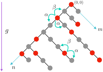
Figure 1: A schematic of the random comb, consisting of a backbone, with random-length branches. Here, $g$ denotes a constant field acting downward, while the quantities $\alpha$ and $\beta$ denote rates with which an ASEP particle hops to a nearest-enighbor site along and opposite to the direction of the field, respectively. The pair of indices ($n,m$) label the sites on the comb, wherein $0\leq n\leq N-1$ labels the backbone sites and $0\leq m\leq L_{n}$ labels the $(L_{n}+1)$ number of sites on the branch attached to the $n$-th backbone site. Presence and absence of red filled circle denote respectively an occupied and an empty site.

Before we move on to discuss the ASEP dynamics on the RC, we recall in the following section the analysis of the dynamics on a $1D$ lattice for use in later parts of the paper.

3 ASEP on a $1D$ lattice

Let us consider the ASEP dynamics on a $1D$ lattice with a given number of sites. Hard-core exclusion implies that the ASEP system can have at most as many particles as is the total number of lattice sites. Let $n_{i}=0,1$ denote the occupation number of the $i$-th lattice site, with $n_{i}=0$ (respectively, $n_{i}=1$) implying that the $i$-th site is empty (respectively, occupied). Defining $W_{j\to i}$ as the hop rate from site $j$ to site $i$, the dynamics in an infinitesimal time interval $[t,t+\mathrm{d}t]$ may then be represented as

$$n_{i}(t+{\mathrm{d}t})-n_{i}(t)=\sum_{j\neq i}W_{j\to i}\,{\mathrm{d}t}\,n_{j}(t)[1-n_{i}(t)]-\sum_{j\neq i}W_{i\to j}\,{\mathrm{d}t}\,[1-n_{j}(t)]n_{i}(t)+\mathcal{O}({\mathrm{d}t}^{2}),$$ (2)

so that in the limit ${\mathrm{d}t}\to 0$, we have

$$\frac{\mathrm{d}n_{i}(t)}{\mathrm{d}t}=\sum_{j}\left(W_{j\to i}n_{j}(t)[1-n_{i}(t)]-W_{i\to j}\,[1-n_{j}(t)]n_{i}(t)\right).$$ (3)

Averaging over dynamical realizations leads to the result

$$\frac{\mathrm{d}\rho_{i}(t)}{\mathrm{d}t}=\sum_{j}\left(W_{j\to i}\langle n_{j}(t)[1-n_{i}(t)]\rangle-W_{i\to j}\,\langle[1-n_{j}(t)]n_{i}(t)\rangle\right),$$ (4)

where $\rho_{i}(t)\equiv\langle n_{i}(t)\rangle$ is the average density on the $i$-th site at time $t$.

It is evident from the structure of Eq. (4) that solving for one-point functions such as $\rho_{i}(t)$ requires knowledge of two-point functions $\langle n_{i}(t)n_{j}(t)\rangle;~i\neq j$, whose solution requires one to solve for three-point functions $\langle n_{i}(t)n_{j}(t)n_{k}(t)\rangle;~i\neq j\neq k$, leading to an infinite hierarchy. Such a hierarchy is broken under the mean-field (MF) approximation, in which any such $n$-point function is factorized into a product of $n$ one-point functions, as in $\langle n_{i}(t)n_{j}(t)n_{k}(t)\ldots n_{p}(t)\rangle=\langle n_{i}(t)\rangle\langle n_{j}(t)\rangle\langle n_{k}(t)\rangle\ldots\langle n_{p}(t)\rangle$ for $i\neq j\neq k\neq\ldots\neq p$. Thus, under the MF approximation, one neglects correlations between the occupancies of different sites at the same time instant. For a $1D$ lattice with hopping rates $\alpha$ and $\beta$ to hop respectively to the right and to the left nearest-neighbour site, one thus obtains from Eq. (4) that

$$\frac{\mathrm{d}\rho_{i}(t)}{\mathrm{d}t}= \left[\alpha\rho_{i-1}(t)+\beta\rho_{i+1}(t)-(\alpha+\beta)\rho_{i}(t)\right]+(\alpha-\beta)\,\left[\rho_{i+1}(t)\rho_{i}(t)-\rho_{i}(t)\rho_{i-1}(t)\right].$$ (5)

The above equation has to be suitably supplemented with information regarding the dynamics at the boundary sites of the lattice.

The MF approximation is known to be exact in the thermodynamic limit (both the particle number and the number of lattice sites approaching infinity, while keeping the ratio fixed and finite) for the ASEP on a $1D$ periodic lattice [42]. Even with open boundaries with particles entering at and leaving from the boundary sites, the MF approximation is known to yield a rather rich phase diagram [47] that, in the thermodynamic limit (both the average particle number and the number of lattice sites approaching infinity, while keeping the ratio fixed and finite), matches perfectly well with the one obtained on the basis of an exact solution [45]; the density profile predicted by the MF however deviates from the one obtained on the basis of the exact solution.

4 ASEP on a random comb: The mean-field (MF) approximation

4.1 Density-evolution equations

We now study the ASEP dynamics on the RC. Denoting by $\rho_{n,m}(t)$ the density on a given site $(n,m)$ at time $t$, the NESS that the system settles at long times $t\to\infty$ has by definition that

$$\frac{\mathrm{d}}{\mathrm{d}t}\rho_{n,m}(t)=0~\,\forall~\,n,m.$$ (6)

We first show that in the stationary state, the branches carry no current. Let us denote by $J_{(n,m-1)\to(n,m)}(t)$ the average of the net current from the site $(n,m-1)$ to the site $(n,m)$ at time $t$. Particle conservation implies that for branch sites ($m\neq 0$), the density evolution takes place according to the equation of continuity in discrete space and continuous time:

$$\frac{\mathrm{d}}{{\mathrm{d}t}}\rho_{n,L_{n}}(t)=J_{(n,L_{n}-1)\to(n,L_{n})}(t);\qquad m=L_{n}~\text{and}~\forall~n=0,1,2,\ldots,N-1,$$ (7a)

$$\frac{\mathrm{d}}{\mathrm{d}t}\rho_{n,m}(t)=J_{(n,m-1)\to(n,m)}(t)-J_{(n,m)\to(n,m+1)}(t);$$

$$\qquad\qquad\qquad\qquad\qquad 0<m<L_{n}~\text{and}~\forall~n=0,1,2,\ldots,N-1.$$ (7b)

In the stationary state, the first equation implies that one has $J^{\rm{st}}_{(n,L_{n}-1)\to(n,L_{n})}=0$, which when used in the second equation with $m=L_{n}-1$ and subsequently for $m=L_{n}-2,L_{n}-3,\ldots,$ implies that the average of the net current is zero for any bond along the branches, or, in other words, the RC branches carry no current in the stationary state. Consequently, one has in the stationary state an average current that is uniform along the backbone.

In terms of the densities, one has

$$J_{(n,m-1)\to(n,m)}(t) \equiv\alpha\,\langle n_{n,m-1}(t)(1-n_{n,m}(t))\rangle-\beta\,\langle n_{n,m}(t)(1-n_{n,m-1}(t))\rangle,$$ (7h)

which under the MF approximation becomes

$$J_{(n,m-1)\to(n,m)}(t) \equiv\alpha\,\rho_{n,m-1}(t)(1-\rho_{n,m}(t))-\beta\,\rho_{n,m}(t)(1-\rho_{n,m-1}(t)).$$ (7i)

Let us now write down the time-evolution equation for the densities under the MF approximation. For branch sites ($m\neq 0$), we have

$$\frac{\mathrm{d}}{{\mathrm{d}t}}\rho_{n,L_{n}}(t) =\alpha\rho_{n,L_{n}-1}(t)-\beta\rho_{n,L_{n}}(t)$$

$$-(\alpha-\beta)\rho_{n,L_{n}-1}(t)~\rho_{n,L_{n}}(t);\qquad m=L_{n}~\text{and}~\forall~n=0,1,2,\ldots,N-1,$$ (7ja)

$$\frac{\mathrm{d}}{\mathrm{d}t}\rho_{n,m}(t) =\alpha\rho_{n,m-1}(t)+\beta\rho_{n,m+1}(t)-(\alpha+\beta)\rho_{n,m}(t)$$

$$-(\alpha-\beta)\rho_{n,m}(t)\left[\rho_{n,m+1}(t)-\rho_{n,m-1}(t)\right];$$

$$\qquad\qquad\qquad\qquad\qquad\qquad 0<m<L_{n}~\text{and}~\forall~n=0,1,2,\ldots,N-1,$$

while for backbone sites ($m=0$), we have

$$\frac{\mathrm{d}}{\mathrm{d}t}\rho_{n,0}(t) =[\alpha\rho_{n-1,0}+\beta\rho_{n+1,0}(t)+\beta\rho_{n,1}(t)-(2\alpha+\beta)\rho_{n,0}(t)]$$

$$+(\alpha-\beta)\rho_{n,0}(t)\left[\rho_{n+1,0}(t)+\rho_{n,1}(t)-\rho_{n-1,0}(t)\right];\qquad 0<n<N-1,$$ (7jka)

$$\frac{\mathrm{d}}{\mathrm{d}t}\rho_{0,0}(t) =[\alpha\rho_{N-1,0}(t)+\beta\rho_{1,0}(t)+\beta\rho_{0,1}(t)-(2\alpha+\beta)\rho_{0,0}(t)]$$

$$+(\alpha-\beta)\rho_{0,0}(t)\left[\rho_{1,0}(t)+\rho_{0,1}(t)-\rho_{N-1,0}(t)\right];\qquad\qquad\qquad\,n=0,$$ (7jkb)

$$\frac{\mathrm{d}}{\mathrm{d}t}\rho_{N-1,0}(t) =[\alpha\rho_{N-2,0}(t)+\beta\rho_{0,0}(t)+\beta\rho_{N-1,1}(t)-(2\alpha+\beta)\rho_{N-1,0}(t)]$$

$$+(\alpha-\beta)\rho_{N-1,0}(t)\left[\rho_{0,0}(t)+\rho_{N-1,1}(t)-\rho_{N-2,0}(t)\right];\qquad n=N-1.$$ (7jkc)

In the stationary state, one has on using Eq. (7ja) that $\alpha\rho_{n,L_{n}-1}-\beta\rho_{n,L_{n}}=(\alpha-\beta)\rho_{n,L_{n}-1}~\rho_{n,L_{n}}$, yielding

$$\rho_{n,L_{n}}=\frac{\rho_{n,L_{n}-1}}{\frac{1}{f}+\left(1-\frac{1}{f}\right)\rho_{n,L_{n}-1}}.$$ (7jkl)

Similarly, Eq. (LABEL:eq:ME_branch) yields in the stationary state that

$$\alpha\rho_{n,m-1}+\beta\rho_{n,m+1}-(\alpha+\beta)\rho_{n,m}=(\alpha-\beta)\rho_{n,m}\left[\rho_{n,m+1}-\rho_{n,m-1}\right];\quad 0<m<L_{n}.$$ (7jkm)

Substituting $m=L_{n}-1$ in the above equation and rearranging, we get

$$\left[1-\left(1-\frac{1}{f}\right)\rho_{n,L_{n}-1}\right]\rho_{n,L_{n}-2}=\left(1+\frac{1}{f}\right)\rho_{n,L_{n}-1}-\left[\left(1-\frac{1}{f}\right)\rho_{n,L_{n}-1}+\frac{1}{f}\right]\rho_{n,L_{n}},$$ (7jkn)

which on using Eq. (7jkl) gives

$$\rho_{n,L_{n}-1}=\frac{\rho_{n,L_{n}-2}}{\frac{1}{f}+\left(1-\frac{1}{f}\right)\rho_{n,L_{n}-2}}.$$ (7jko)

The above equation relates the stationary-state densities between sites at distances $1$ and $2$ units from the reflecting end of the $n$-th branch. Next, using $m=L_{n}-2$ in Eq. (7jkm), and using Eq. (7jko), one obtains

$$\rho_{n,L_{n}-2}=\frac{\rho_{n,L_{n}-3}}{\frac{1}{f}+(1-\frac{1}{f})\rho_{n,L_{n}-3}}.$$ (7jkp)

In this way, substituting successively for different values of $m$ in Eq. (7jkm), we obtain a relation between the stationary-state densities on two consecutive sites $(n,m)$ and $(n,m-1)$ on a branch, as

$$\rho_{n,m}=\frac{\rho_{n,m-1}}{\frac{1}{f}+\left(1-\frac{1}{f}\right)\rho_{n,m-1}};\qquad 1\leq m\leq L_{n},$$ (7jkq)

leading finally to

$$\frac{1}{\rho_{n,m}}=1+\frac{1}{f^{m}}\left(\frac{1}{\rho_{n,0}}-1\right).$$ (7jkr)

The above equation relates the stationary-state density on any branch site to that on the corresponding backbone site.

We now turn to the stationary-state densities on backbone sites. Equation (7jka) gives in the stationary state that for $0<n<N-1$, one has

$$\left[\rho_{n-1,0}+\frac{1}{f}\rho_{n+1,0}-\left(2+\frac{1}{f}\right)\rho_{n,0}\right]+\left(1-\frac{1}{f}\right)\rho_{n,0}\left[\rho_{n+1,0}-\rho_{n-1,0}\right]$$

$$+\Big{(}\frac{1}{f}+\left(1-\frac{1}{f}\right)\rho_{n,0}\Big{)}\rho_{n,1}=0.$$ (7jks)

Substituting for $\rho_{n,1}$ from Eq. (7jkq) in Eq. (7jks), we get

$$\left[\rho_{n-1,0}+\frac{1}{f}\rho_{n+1,0}-\left(1+\frac{1}{f}\right)\rho_{n,0}\right]+\left(1-\frac{1}{f}\right)\rho_{n,0}\left[\rho_{n+1,0}-\rho_{n-1,0}\right]=0.$$ (7jkt)

Similarly, using Eqs. (7jkb) and (7jkc), we get

$$\left[\rho_{N-1,0}+\frac{1}{f}\rho_{1,0}-\left(1+\frac{1}{f}\right)\rho_{0,0}\right]+\left(1-\frac{1}{f}\right)\rho_{0,0}\left[\rho_{1,0}-\rho_{N-1,0}\right]=0,\qquad n=0,$$ (7jkua)

$$\left[\rho_{N-2,0}+\frac{1}{f}\rho_{0,0}-\left(1+\frac{1}{f}\right)\rho_{N-1,0}\right]+\left(1-\frac{1}{f}\right)\rho_{N-1,0}\left[\rho_{0,0}-\rho_{N-2,0}\right]=0,~\,n=N-1.$$ (7jkub)

We have obtained a remarkable result: Eqs. (7jkt), 7jkua) and 7jkub) (i) are independent of $L_{n}$, and, moreover, (ii) are equivalent to those with $L_{n}=0$. The latter means more specifically that Eqs. (7jkt), 7jkua) and 7jkub) are mathematically equivalent to those for stationary-state single-site densities $\sigma_{n}^{\mathrm{st}};~n=0,1,\ldots,N-1$ for ASEP particles undergoing hopping to nearest-neighbor sites on a $1D$ periodic lattice of $N$ sites, with $\alpha$ and $\beta$ being the forward and the backward hopping rate. This aforementioned equivalence with respect to ASEP dynamics on a $1D$ lattice holds only for stationary-state single-site densities, and holds despite the fact that the underlying dynamics includes backbone and branch sites and involves hopping between them. We will later use this equivalence to obtain analytical results on the stationary-state transport properties of the ASEP particles on the comb. The stationary-state density equation being equivalent yields in both cases a uniform density: uniform ($\rho_{n,0}=\rho^{\mathrm{st}}~\forall~n$) over the backbone sites, and uniform ($={\sigma}^{\mathrm{st}}$) over the $1D$ periodic lattice. However, the total number of ASEP particles $\mathcal{N}$ being conserved in both cases, the normalization condition for the stationary-state density reads differently. Indeed, one has $\sum_{n=0}^{N-1}\sum_{m=0}^{L_{n}}\rho_{n,m}=\mathcal{N}$ for the comb, whereas for the periodic lattice, one has instead that $\sum_{n=0}^{N-1}\sigma^{\mathrm{st}}=\mathcal{N}$.

Using Eq. (7jkr) in the normalization condition $\sum_{n=0}^{N-1}\sum_{m=0}^{L_{n}}\rho_{n,m}=\mathcal{N}$ gives

$$\sum_{n=0}^{N-1}\sum_{m=0}^{L_{n}}\left[1+\frac{1}{f^{m}}\left(\frac{1}{\rho^{\mathrm{st}}}-1\right)\right]^{-1}=\mathcal{N}.$$ (7jkuv)

One now requires to solve the above algebraic equation numerically, the root of which yields the stationary-state uniform density $\rho^{\mathrm{st}}$ on the comb-backbone. Knowing $\rho^{\mathrm{st}}$, the stationary-state branch-site densities can be readily obtained from Eq. (7jkr) as

$$\rho_{n,m}=\left[1+\frac{1}{f^{m}}\left(\frac{1}{\rho^{\mathrm{st}}}-1\right)\right]^{-1}.$$ (7jkuw)

We thus note that although in the stationary state, the densities are uniform over the backbone, the same on the branches are not at all uniform. The above equation appears independent of branch-lengths $L_{n}$, but actually depends on all of them via Eq. (7jkuv). Equation (7jkuw) also shows how the stationary-state densities are distributed on a branch, being lowest on the corresponding backbone site and highest at the branch end point. Longer the branch, higher are the densities towards the branch end. Explicitly, consider two branches of lengths $L_{n_{1}}$ and $L_{n_{2}}$ attached to backbone sites $n_{1}$ and $n_{2}$, respectively, with $L_{n_{1}}>L_{n_{2}}$. Then, one can show on using Eq. (7jkuw) that

$$\frac{1}{\rho_{n_{1},L_{n_{1}}}}-\frac{1}{\rho_{n_{2},L_{n_{2}}}}=\left[\frac{1}{f^{L_{n_{1}}}}-\frac{1}{f^{L_{n_{2}}}}\right]\left(\frac{1}{\rho^{\mathrm{st}}}-1\right)<0,$$ (7jkux)

i.e., $\rho_{n_{1},L_{n_{1}}}>\rho_{n_{2},L_{n_{2}}}$.

4.2 Stationary-state transport properties

We now proceed to obtain the transport properties of our system in the stationary state. We are particularly interested in the drift velocity along the backbone, defined as the velocity, computed along the backbone, of a particle (any particle) performing the ASEP dynamics on the RC. One may operationally define this velocity thus: once the system has settled into the stationary state, locate the different ASEP particles on the lattice and measure for each the distance it covers along the backbone over a large time duration in a typical realization of the dynamics. Summing these distances and dividing by the product of the time duration and the total number of particles yield the drift velocity for the given dynamical realization; Averaging over dynamical realizations then yields the stationary-state drift velocity we are interested in.

Let us denote by $v^{\mathrm{st}}_{\mathrm{{drift}}}$ the stationary-state drift velocity. To proceed, consider the stationary-state-equivalent problem of the ASEP dynamics on a $1D$ periodic lattice that we discussed in the preceding subsection. Evidently, the average current across any bond $(i,i+1)$ will be the same for every bond in the stationary state, and will be given by $J^{\mathrm{st}}_{\mathrm{{drift}}}=(\alpha-\beta)\langle\sigma_{i}(1-\sigma_{i+1})\rangle_{\mathrm{st}}$, where $\sigma_{i}=0,1$ denotes respectively the absence and the presence of an ASEP particle on the $i$-th site, and the angular brackets denote averaging with respect to the stationary-state measure. Under the MF approximation, one has $J^{\mathrm{st}}_{\mathrm{{drift}}}=(\alpha-\beta)\langle\sigma_{i}\rangle_{\mathrm{st}}\langle(1-\sigma_{i+1})\rangle_{\mathrm{st}}=(\alpha-\beta)\sigma^{\mathrm{st}}(1-\sigma^{\mathrm{st}})$, using the fact that the stationary state corresponds to a uniform density over the lattice. We thus immediately obtain the stationary-state drift velocity in this equivalent ASEP problem as $v^{\mathrm{st}}_{\mathrm{{drift}}}=J^{\mathrm{st}}_{\mathrm{{drift}}}/\sigma^{\mathrm{st}}=(\alpha-\beta)\,(1-\sigma^{\mathrm{st}})$. Using the equivalence unveiled in the preceding subsection between the stationary-state single-site densities for the RC backbone and that for an ASEP on a $1D$ periodic lattice, we thus obtain for our problem on the random comb that the stationary-state current along the backbone equals $J^{\mathrm{st}}_{\mathrm{{drift}}}=(\alpha-\beta)\rho^{\mathrm{st}}(1-\rho^{\mathrm{st}})$.

Before proceeding to obtain an expression for $v^{\mathrm{st}}_{\mathrm{{drift}}}$, we now demonstrate that in the stationary state, the average current in the branches is identically zero under the MF approximation; we have

$$J_{(n,m-1)\to(n,m)}^{\mathrm{st}} \equiv\alpha\,\rho_{n,m-1}(1-\rho_{n,m})-\beta\,\rho_{n,m}(1-\rho_{n,m-1}).$$ (7jkuy)

Substituting for $\rho_{n,m}$ from Eq. (7jkq), one arrives at the result: $J_{(n,m-1)\to(n,m)}^{\mathrm{st}}=0,~\,\forall~\,m>0,n$.

Since, as argued above, the branches do not contribute to the stationary current on the comb, we get $J^{\mathrm{st}}_{\mathrm{{drift}}}/\rho_{\mathrm{tot}}$ as the drift velocity on the RC, taking into account displacements along both the backbone and the branches. However, recalling that $v^{\mathrm{st}}_{\mathrm{{drift}}}$, the quantity of interest, considers displacements only along the backbone, we may relate the two drift velocities by simply equating the time for the respective displacements, as

$$\frac{N}{v^{\mathrm{st}}_{\mathrm{{drift}}}}=\frac{N+\sum_{n=0}^{N-1}L_{n}}{(J^{\mathrm{st}}_{\mathrm{{drift}}}/\rho_{\mathrm{tot}})},$$ (7jkuz)

where we may recall that all our lattice spacings have been taken to be unity. Rearranging, we get

$$v^{\mathrm{st}}_{\mathrm{{drift}}}=p\frac{J^{\mathrm{st}}_{\mathrm{{drift}}}}{\rho_{\mathrm{tot}}}=(\alpha-\beta)\,p\,\frac{\rho^{\mathrm{st}}(1-\rho^{\mathrm{st}})}{\rho_{\mathrm{tot}}}=2Wg\,p\,\frac{\rho^{\mathrm{st}}(1-\rho^{\mathrm{st}})}{\rho_{\mathrm{tot}}},$$ (7jkuaa)

where $p\equiv N/\left(N+\sum_{n=0}^{N-1}L_{n}\right)$ is the fraction of the total number of sites that constitute the backbone. Note that $\rho_{\mathrm{tot}}$ and $p$ are random variables varying between realizations of the RC.

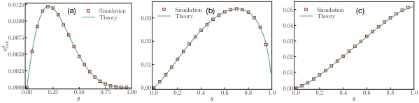
Figure 2: Shown in panels (a) – (c) is the stationary-state drift velocity versus bias $g$ at various values of the total ASEP particle density $\rho_{\mathrm{tot}}$, as obtained from theory (Eq. (7jkuaa), continuous line) and numerics (symbols), with number of backbone sites $N=100$ and for a typical disorder realization of the comb. The realization of the comb being fixed, varying $\rho_{\mathrm{tot}}$ is tantamount to varying the total number of particles in the system. The branch-lengths are sampled independently from the exponential distribution (1) with $M=20$ and $\xi=5$. The number of particles is $\mathcal{N}=200$ [panel (a)], $400$ [panel (b)] and $450$ [panel (c)], whereas the total number of sites on the comb is $513$. Numerics correspond to Monte Carlo simulations of the dynamics as detailed in A; the displayed data correspond to the stationary state.

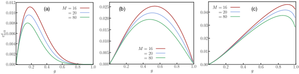
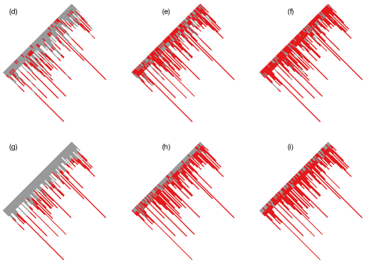
Figure 3: Panels (a) – (c) show the behavior of stationary-state drift velocity with bias $g$ for three different ASEP particle density, $\rho_{\mathrm{tot}}=0.35$, $0.70$, and $0.85$, respectively. Data are obtained from theory (Eq. (7jkuaa)), with number of backbone sites $N=10^{4}$, and for a typical realization of the random comb. The branch lengths are sampled independently from the exponential distribution (1) with $\xi=5$ and $M=16,20,80$. The pair of panels ((d),(g)), ((e),(h)) and ((f),(i)) show for the same values of $\rho_{\mathrm{tot}}$ (or, equivalently $\mathcal{N}$), $M$, $\xi$ as for Fig. 2(a), (b), (c), respectively, a stationary-state (i.e., at long times $t=4\times 10^{5}$) snapshot of the random comb, with red representing occupied sites and gray denoting unoccupied ones, at a low bias $g=0.2$ and a high bias $g=0.8$, respectively.

We verify our result (7jkuaa) with Monte Carlo simulation results at low as well as high ASEP particle density $\rho_{\mathrm{tot}}$, see Fig. 2. Details of the simulation procedure are given in A. Note that in both simulations and displayed theoretical results in this paper, we take $W=1/2$, unless stated otherwise. In simulations for a fixed RC realization, note that varying particle density is tantamount to varying the total number $\mathcal{N}$ of particles in the system. Figure 3, panels (a) – (c), show for three values of $\rho_{\mathrm{tot}}$, low, intermediate and high, our theoretical results on the variation of $v^{\mathrm{st}}_{\mathrm{{drift}}}$ with $g$; in each case, we have considered three values of $M$. Let us now discuss the displayed results. For fixed values of $N$ (taken to be very large, $N=10^{4}$), $M$, and $\xi$, the most evident feature seen in panels (a) – (c) is the following: at a fixed $g$, as $\rho_{\mathrm{tot}}$ increases, so does the drift velocity. Consequently, the variation of $v^{\mathrm{st}}_{\mathrm{{drift}}}$ with $g$ becomes more and more monotonic as $\rho_{\mathrm{tot}}$ increases beyond a threshold value. Moreover, as $M$ becomes larger, this threshold value for $\rho_{\mathrm{tot}}$ also increases. For given values of $N$, $M$, $\xi$, as $\rho_{\mathrm{tot}}\to 0$, the behavior of the drift velocity versus $g$ is expected to be the one reported earlier for the case of non-interacting particles undergoing biased hopping on the RC [4], implying a non-motonic dependence and existence of a critical $g$ beyond which the drift velocity becomes zero.

In order to understand physically the aforementioned features for Fig. 2, panels (a) – (c), we now do the following. For panel 2(a), we show in panels (d) and (g) of Fig. 3, a typical snapshot of the configuration of the system at late times (i.e., in the stationary state) and for same values of $\rho_{\mathrm{tot}}$ (or, equivalently, the total particle number $\mathcal{N}$), $M$, $\xi$ as in panel 2(a), but with respectively two different values of bias $g$, one low and one high. We see that at a given $g$, the particles undergoing biased hopping in the direction of the bias fill up the branches, which in our RC all run along the direction of the bias. Once the branches get filled up, particles especially towards the end of the branches find it difficult to move back to the backbone. This is owing to the combined effect of the requirement behind such a move to hop against the bias (which occurs with a smaller rate relative to hops in the direction of the bias) and the presence of hard-core exclusion. The longer the branch, the higher is the probability that more particles towards the end of the branch are trapped. Consequently, only a few particles on the backbone and near the intersection of the backbone with the branches are mobile; let us denote this region by $\mathcal{R}$. This effect gets pronounced with increase of $g$, when even fewer particles in region $\mathcal{R}$ are mobile. This is seen by comparing region $\mathcal{R}$ in panels (d) and (g), when one finds in the latter panel fewer red dots in region $\mathcal{R}$ compared to the former panel. Repeating the exercise performed above for panel 2(a) also for panels 2(b) and 2(c), we may arrive at a similar conclusion by comparing the snapshots in panels (e),(h) and (f),(i), of Fig. 3 respectively. Of course, with increase of $\rho_{\mathrm{tot}}$, one has in region $\mathcal{R}$ more particles as one moves from panels (d) to (e) to (f) and from panels (g) to (h) to (i).

On the basis of the above, we conclude that as $\rho_{\mathrm{tot}}$ increases, keeping $g$, $M$, $\xi$ fixed, the branches become less participatory in the dynamics, and it is only the mobile particles in region $\mathcal{R}$ (whose number increases with increasing $\rho_{\mathrm{tot}}$) that contribute to $v^{\mathrm{st}}_{\mathrm{{drift}}}$. These latter particles cannot get trapped, as the effects of branches are largely absent. Consequently, the variation of $v^{\mathrm{st}}_{\mathrm{{drift}}}$ with $g$ becomes more and more monotonic as $\rho_{\mathrm{tot}}$ increases beyond a threshold value. An estimate of the latter would be the density corresponding to all branch sites filled up, given by the ratio $\sum_{n=0}^{N-1}L_{n}/(N+\sum_{n=0}^{N-1}L_{n})$.

4.3 On the validity of the MF approximation

Because of the inherent spatial inhomogeneity, translational invariance does not hold for the RC. Particles tend to get clustered towards the free end of the branches, thereby increasing the correlation between the occupancy of nearest-neighbor sites, especially when the particle density and the bias are both high. Hence, whether a mean-field approximation is able to efficiently capture the dynamics is a priori not obvious. We have seen in the previous subsection and particularly in Fig. 2 that results based on the MF approximation match quite with simulation results. To address the question of validity of the MF approximation, we compute numerically the two-point correlation, specifically, the quantity

$$\Delta\equiv\frac{\langle n_{i}n_{i+1}\rangle}{\langle n_{i}\rangle^{2}}-1$$ (7jkuab)

over the entire comb and for various values of $g$ and $\rho_{\mathrm{tot}}$ (i.e., for different total number of particles) for a given realization of the RC. One expects $\Delta\to 0$ as a signature of the validity of the MF approximation. Figure (4) shows that quite remarkably, one observes $\Delta$ in the stationary state to deviate significantly from zero, especially on the branches. Nonetheless, at least for the stationary-state drift velocity, we have seen that the agreement between results based on the MF approximation and Monte Carlo simulations is quite good.

We now argue that despite $\Delta$ being significantly different from zero, why the MF approximation predicts correctly the stationary-state drift velocity. We have already shown in Section 4.1 that the stationary state corresponds to zero average current in the branches of the RC. Further, we have shown in Section 4.2 that the MF approximation ensures this zero-current condition and hence would predict a possible stationary state of the system. But the system being ergodic has a unique stationary state, as argued in Section 2. Hence, the stationary state predicted by the MF approximation is this unique stationary state of the system, and this explains the perfect agreement between MF-approximation and numerical-simulation results for the stationary-state drift velocity as displayed in Fig. 2.

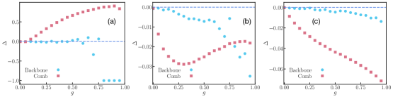
Figure 4: (a) For a typical RC realization, the figure shows the quantity $\Delta$ in Eq. (7jkuab) against the bias $g$ for various values of the total ASEP particle density $\rho_{\mathrm{tot}}$, from low [panel (a)], through intermediate [panel (b)], to high [panel (c)] values. Numerics correspond to Monte Carlo simulations of the dynamics, details of which may be found in A. The various parameter values and the RC realization are the same as in Fig. 2.

5 Summary and conclusions

In this work, we studied using a mean-field approximation the stationary-state static and dynamic properties of particles with hard-core interactions undergoing asymmetric simple exclusion process (ASEP) on a random comb (RC). The RC comprises a backbone lattice from each site of which emanates a branch with a random number of sites. The particles undergo hopping in presence of a bias, with hopping to nearest-neighbor sites that are empty are more likely in the direction of the bias than in the opposite direction. The backbone and the branches run in the direction of the bias. The number of branch sites or alternatively the branch lengths are sampled independently from a common distribution, specifically, an exponential distribution. Our results show that the stationary-state density is uniform along the backbone and nonuniform along the branches, decreasing monotonically from the free-end of a branch to its intersection with the backbone. On the other hand, the drift velocity of particles along the backbone when studied as a function of the bias strength exhibits a non-monotonic dependence, which remarkably becomes increasingly monotonic as one increases the ASEP particle density. This effect is a manifestation of an effective reduction of the branch lengths and a motion of the particles that takes place primarily along the backbone, owing to an intricate interplay between hard-core interactions and biased hopping. It is left as a future exercise to analyze in further detail the range of applicability of the mean-field approximation, by considering branch-length distribution other than the studied exponential distribution, and for geometries other than the studied random network. Introducing stochastic resetting  [48, 49] in the dynamics is also an interesting future direction worth taking up, an issue that was studied by us recently in the absence of any interaction between the particles and was shown to lead to nontrivial results of relevance [6].

6 Acknowledgements

This project is supported by the Deutsche Forschungsgemeinschaft (DFG, German Research Foundation) under Germany’s Excellence Strategy EXC 2181/1-390900948 (the Heidelberg STRUCTURES Excellence Cluster). M.S. also acknowledges support by the state of Baden-Württemberg through bwHPC cluster. S.G. acknowledges computational resources of the Department of Theoretical Physics, TIFR, assistance of Kapil Ghadiali and Ajay Salve, and financial support of Department of Atomic Energy, Government of India, under Project Identification No. RTI 4002.

Appendix A Details of Monte Carlo simulations

Here, we discuss a Monte Carlo simulation algorithm to simulate the ASEP dynamics on a given realization of the random comb. We first need to generate the comb. This is done by deciding on the number of backbone sites (call it $N$) and the branch-length cut-off $M$, and then drawing independently for each backbone site the corresponding branch length $L_{n}$ from the exponential distribution $\mathcal{P}_{L}$ in Eq. (1). We next choose specific values of the total number of ASEP particles $\mathcal{N}(\leq N+\sum_{n=0}^{N-1}L_{n})$, the bias $g$, and the parameter $W$. As mentioned in the main text, the lattice spacing is taken to be unity. As representative choices to perform our simulations, we take $N=100$, $M=20$, and $W=0.5$, unless stated otherwise.

A typical simulation involves initializing the dynamics at time $t=0$ with $\mathcal{N}$ particles distributed randomly on various RC-sites $(n,m)$, and letting them perform the ASEP dynamics with chosen value of the time step $\mathrm{d}t$. Given the position of a particle at time $t$, in the ensuing infinitesimal time interval $[t,t+\mathrm{d}t]$, the position of the particle is updated as follows (provided of course that when the attempt of a particle to move away from its current location is accepted, the particle can actually hop into the destination site provided the latter is unoccupied):

1. If at time $t$ the particle is on a branch site that is not the end site of the branch, it attempts to move along the branch with equal probability of $1/3$ in either along or opposite to the direction of the bias, while it attempts to stay put with probability $1/3$. The move in the direction of the bias is actually accepted with probability $(3/2)(1+g)\mathrm{d}t$, while the move opposite to the direction of the bias is accepted with probability $(3/2)(1-g)\mathrm{d}t$.

2. If at time $t$ the particle is on the end site (the reflecting end) of the branch, it attempts to move along the branch and in the direction opposite to the bias with probability $1/3$, while it attempts to stay put with probability $2/3$. The move opposite to the direction of the bias is successful with probability $(3/2)(1-g)\mathrm{d}t$.

3. If at time $t$ the particle is on a backbone site with no branch attached, it decides to move along the backbone either along or opposite to the direction of the bias with equal probability of $1/3$, while it stays put with probability $1/3$. The moves in the direction of and opposite to the direction of the bias are accepted respectively with probabilities $(3/2)(1+g)\mathrm{d}t$ and $(3/2)(1-g)\mathrm{d}t$.

4. If at time $t$ the particle is on a backbone site with a branch attached to it, it decides to move along the backbone either along or opposite to the direction of the bias with equal probability of $1/3$, while it decides to move into the attached branch site with probability $1/3$. The moves in the direction of and opposite to the direction of the bias are accepted respectively with probabilities $(3/2)(1+g)\mathrm{d}t$ and $(3/2)(1-g)\mathrm{d}t$. The move to the branch site is accepted with probability $(3/2)(1+g)\mathrm{d}t$.

One Monte Carlo time step of the dynamics corresponds to choosing for $\mathcal{N}$ number of times the ASEP particles at random, and updating their current location following the above-mentioned rules. We keep evolving the dynamics for a long time until it settles into a stationary state, and measure the stationary-state drift velocity in the following way.

In the stationary state, all the $\mathcal{N}$ particles are tracked for a long observation time $T$. We compute first the velocity of the individual particles, ($v[i];\,i=1,2,\dots,\mathcal{N}$), along the backbone and in the direction of the bias as follows:

$$v[i]=\frac{\begin{subarray}{c}\text{Net displacement of the $i$-th particle on the backbone}\\ \text{and in the direction of the bias in time}~T\end{subarray}}{T}.$$ (7jkuac)

Finally, the stationary-state drift velocity is computed as

$$v^{\mathrm{st}}_{\mathrm{{drift}}}=\frac{1}{\mathcal{N}}\sum_{i=1}^{\mathcal{N}}v[i].$$ (7jkuad)

References

- Evans et al. [1998] M R Evans, Yariv Kafri, H M Koduvely, and David Mukamel. Phase separation in one-dimensional driven diffusive systems. Physical Review Letters, 80(3):425, 1998.
- Evans et al. [1995] Martin R Evans, Damien P Foster, Claude Godrèche, and David Mukamel. Spontaneous symmetry breaking in a one dimensional driven diffusive system. Physical Review Letters, 74(2):208, 1995.
- Barma and Dhar [1983] Mustansir Barma and Deepak Dhar. Directed diffusion in a percolation network. Journal of Physics C: Solid State Physics, 16(8):1451, 1983.
- White and Barma [1984] Steven R White and Mustansir Barma. Field-induced drift and trapping in percolation networks. Journal of Physics A: Mathematical and General, 17(15):2995, 1984.
- Dhar [1984] Deepak Dhar. Diffusion and drift on percolation networks in an external field. Journal of Physics A: Mathematical and General, 17(5):L257, 1984.
- Sarkar and Gupta [2022] Mrinal Sarkar and Shamik Gupta. Biased random walk on random networks in presence of stochastic resetting: Exact results. Journal of Physics A: Mathematical and Theoretical, 55(42):42LT01, 2022.
- Havlin et al. [1987] Shlomo Havlin, James E Kiefer, and George H Weiss. Anomalous diffusion on a random comblike structure. Physical Review A, 36(3):1403, 1987.
- Pottier [1995] Noëlle Pottier. Diffusion on random comblike structures: field-induced trapping effects. Physica A: Statistical Mechanics and its Applications, 216(1-2):1–19, 1995.
- Bunde et al. [1986] A Bunde, S Havlin, H E Stanley, B Trus, and G H Weiss. Diffusion in random structures with a topological bias. Physical Review B, 34(11):8129, 1986.
- Balakrishnan and Van den Broeck [1995] V Balakrishnan and C Van den Broeck. Transport properties on a random comb. Physica A: Statistical Mechanics and its Applications, 217(1-2):1–21, 1995.
- Stauffer [1979] Dietrich Stauffer. Scaling theory of percolation clusters. Physics Reports, 54(1):1–74, 1979.
- Rammal and Toulouse [1983] Rammal Rammal and Gérard Toulouse. Random walks on fractal structures and percolation clusters. Journal de Physique Lettres, 44(1):13–22, 1983.
- Sahimi [1993] Muhammad Sahimi. Flow phenomena in rocks: from continuum models to fractals, percolation, cellular automata, and simulated annealing. Reviews of Modern Physics, 65(4):1393, 1993.
- Méndez and Iomin [2013] Vicenç Méndez and Alexander Iomin. Comb-like models for transport along spiny dendrites. Chaos, Solitons & Fractals, 53:46–51, 2013.
- Cecchi and Magnasco [1996] Guillermo A Cecchi and Marcelo O Magnasco. Negative resistance and rectification in brownian transport. Physical Review Letters, 76(11):1968, 1996.
- Iomin [2012] Alexander Iomin. Superdiffusive comb: Application to experimental observation of anomalous diffusion in one dimension. Physical Review E, 86(3):032101, 2012.
- Agliari et al. [2014] Elena Agliari, Alexander Blumen, and Davide Cassi. Slow encounters of particle pairs in branched structures. Physical Review E, 89(5):052147, 2014.
- Bénichou et al. [2015] O Bénichou, P Illien, G Oshanin, A Sarracino, and R Voituriez. Diffusion and subdiffusion of interacting particles on comblike structures. Physical Review Letters, 115(22):220601, 2015.
- Iomin [2006] A Iomin. Toy model of fractional transport of cancer cells due to self-entrapping. Physical Review E, 73(6):061918, 2006.
- Campos et al. [2006] Daniel Campos, Joaquim Fort, and Vicenç Méndez. Transport on fractal river networks: Application to migration fronts. Theoretical Population Biology, 69(1):88–93, 2006.
- Derrida [1998] Bernard Derrida. An exactly soluble non-equilibrium system: the asymmetric simple exclusion process. Physics Reports, 301(1-3):65–83, 1998.
- Schütz [2001] Gunter M Schütz. Exactly solvable models for many-body systems far from equilibrium. In Phase transitions and critical phenomena, volume 19, pages 1–251. Elsevier, 2001.
- Spitzer [1991] Frank Spitzer. Interaction of markov processes. In Random Walks, Brownian Motion, and Interacting Particle Systems: A Festschrift in Honor of Frank Spitzer, pages 66–110. Springer, 1991.
- Liggett [2013] Thomas M Liggett. Stochastic interacting systems: contact, voter and exclusion processes, volume 324. Springer Science & Business Media, 2013.
- MacDonald et al. [1968] Carolyn T MacDonald, Julian H Gibbs, and Allen C Pipkin. Kinetics of biopolymerization on nucleic acid templates. Biopolymers: Original Research on Biomolecules, 6(1):1–25, 1968.
- Parmeggiani et al. [2003] Andrea Parmeggiani, Thomas Franosch, and Erwin Frey. Phase coexistence in driven one-dimensional transport. Physical Review Letters, 90(8):086601, 2003.
- Neri et al. [2011] Izaak Neri, Norbert Kern, and Andrea Parmeggiani. Totally asymmetric simple exclusion process on networks. Physical Review Letters, 107(6):068702, 2011.
- Neri et al. [2013] Izaak Neri, Norbert Kern, and Andrea Parmeggiani. Modeling cytoskeletal traffic: an interplay between passive diffusion and active transport. Physical Review Letters, 110(9):098102, 2013.
- Chowdhury et al. [2000] Debashish Chowdhury, Ludger Santen, and Andreas Schadschneider. Statistical physics of vehicular traffic and some related systems. Physics Reports, 329(4-6):199–329, 2000.
- Antal and Schütz [2000] Tibor Antal and G M Schütz. Asymmetric exclusion process with next-nearest-neighbor interaction: Some comments on traffic flow and a nonequilibrium reentrance transition. Physical Review E, 62(1):83, 2000.
- Nagatani [2001] Takashi Nagatani. Dynamical transition and scaling in a mean-field model of pedestrian flow at a bottleneck. Physica A: Statistical Mechanics and Its Applications, 300(3-4):558–566, 2001.
- Ono et al. [2002] K Ono, D G Austing, Y Tokura, and S Tarucha. Current rectification by pauli exclusion in a weakly coupled double quantum dot system. Science, 297(5585):1313–1317, 2002.
- Pronina and Kolomeisky [2004] Ekaterina Pronina and Anatoly B Kolomeisky. Two-channel totally asymmetric simple exclusion processes. Journal of Physics A: Mathematical and General, 37(42):9907, 2004.
- Krug [1991] Joachim Krug. Boundary-induced phase transitions in driven diffusive systems. Physical Review Letters, 67(14):1882, 1991.
- Janowsky and Lebowitz [1992] Steven A Janowsky and Joel L Lebowitz. Finite-size effects and shock fluctuations in the asymmetric simple-exclusion process. Physical Review A, 45(2):618, 1992.
- Popkov et al. [2003] Vladislav Popkov, Attila Rákos, Richard D Willmann, Anatoly B Kolomeisky, and Gunter M Schütz. Localization of shocks in driven diffusive systems without particle number conservation. Physical Review E, 67(6):066117, 2003.
- Hinsch and Frey [2006] Hauke Hinsch and Erwin Frey. Bulk-driven nonequilibrium phase transitions in a mesoscopic ring. Physical Review Letters, 97(9):095701, 2006.
- Kafri et al. [2002] Yariv Kafri, Erel Levine, David Mukamel, Gunter M Schütz, and J Török. Criterion for phase separation in one-dimensional driven systems. Physical Review Letters, 89(3):035702, 2002.
- Blythe and Evans [2007] Richard A Blythe and Martin R Evans. Nonequilibrium steady states of matrix-product form: a solver’s guide. Journal of Physics A: Mathematical and Theoretical, 40(46):R333, 2007.
- Ramaswamy and Barma [1987] Ramakrishna Ramaswamy and Mustansir Barma. Transport in random networks in a field: interacting particles. Journal of Physics A: Mathematical and General, 20(10):2973, 1987.
- Iyer et al. [2025] Chandrashekar Iyer, Mustansir Barma, Hunnervir Singh, and Deepak Dhar. Asymmetric simple exclusion process on the percolation cluster: Waiting time distribution in side branches. Physical Review Letters, 134(2):027102, 2025.
- Golinelli and Mallick [2006] Olivier Golinelli and Kirone Mallick. The asymmetric simple exclusion process: an integrable model for non-equilibrium statistical mechanics. Journal of Physics A: Mathematical and General, 39(41):12679, 2006.
- Brankov et al. [2004] Jordan Brankov, Nina Pesheva, and Nadezhda Bunzarova. Totally asymmetric exclusion process on chains with a double-chain section in the middle: Computer simulations and a simple theory. Physical Review E—Statistical, Nonlinear, and Soft Matter Physics, 69(6):066128, 2004.
- Embley et al. [2009] Ben Embley, Andrea Parmeggiani, and Norbert Kern. Understanding totally asymmetric simple-exclusion-process transport on networks: Generic analysis via effective rates and explicit vertices. Physical Review E—Statistical, Nonlinear, and Soft Matter Physics, 80(4):041128, 2009.
- Derrida et al. [1993] Bernard Derrida, Martin R Evans, Vincent Hakim, and Vincent Pasquier. Exact solution of a 1d asymmetric exclusion model using a matrix formulation. Journal of Physics A: Mathematical and General, 26(7):1493, 1993.
- Ishiguro and Sato [2024] Yuki Ishiguro and Jun Sato. Exact steady states in the asymmetric simple exclusion process beyond one dimension. Physical Review Research, 6(3):033030, 2024.
- Derrida et al. [1992] Bernard Derrida, Eytan Domany, and David Mukamel. An exact solution of a one-dimensional asymmetric exclusion model with open boundaries. Journal of Statistical Physics, 69:667–687, 1992.
- Evans et al. [2020] Martin R Evans, Satya N Majumdar, and Grégory Schehr. Stochastic resetting and applications. Journal of Physics A: Mathematical and Theoretical, 53(19):193001, 2020.
- Gupta and Jayannavar [2022] Shamik Gupta and Arun M Jayannavar. Stochastic resetting: A (very) brief review. Frontiers in Physics, 10:789097, 2022.