Exploring the BSM parameter space with Neural Network aided Simulation-Based Inference

Abstract

Some of the issues that make sampling parameter spaces of various beyond the Standard Model (BSM) scenarios computationally expensive are the high dimensionality of the input parameter space, complex likelihoods, and stringent experimental constraints. In this work, we explore likelihood-free approaches, leveraging neural network-aided Simulation-Based Inference (SBI) to alleviate this issue. We focus on three amortized SBI methods: Neural Posterior Estimation (NPE), Neural Likelihood Estimation (NLE), and Neural Ratio Estimation (NRE) and perform a comparative analysis through the validation test known as the Test of Accuracy with Random Points (TARP), as well as through posterior sample efficiency and computational time. As an example, we focus on the scalar sector of the phenomenological minimal supersymmetric SM (pMSSM) and observe that the NPE method outperforms the others and generates correct posterior distributions of the parameters with a minimal number of samples. The efficacy of this framework will be more evident with additional experimental data, especially for high dimensional parameter space.

1 Introduction

The biggest question currently plaguing the High Energy Physics (HEP) community is the nature of new physics beyond the Standard Model (BSM). There are various categories of new physics scenarios all of which are well motivated from different theoretical and phenomenological perspectives, such as, neutrino oscillation  deSalas:2020pgw ; NOvA:2019cyt , possible existence of Dark Matter (DM)  2009GReGr..41..207Z ; 1937ApJ….86..217Z ; Jungman:1995df , hierarchy problem SUSSKIND1984181 ; PhysRevD.14.1667 , CP violation BaBar:2015gfp ; PhysRevD.108.012008 ; Belle:2022uod ; Miao:2023cvk , to name a few. There exist different classes of new physics models that can account for these shortcomings of the SM. These models introduce handful of new parameters and unless they are well constrained, prediction of the experimental observables would not be very unique. So, a major objective of phenomenological studies is to narrow down the possible values of these parameters as much as possible, using both theoretical calculations and experimental observations. Scalar search is of major interest as far as experimental probe of BSM physics is concerned. A lot of BSM scenarios predict the existence of new scalars in addition to the 125 GeV Higgs CMS:2012qbp ; ATLAS:2012yve . A simple example of such extensions would be the two Higgs doublet models (2HDM) Branco:2011iw . One can use the mass and coupling measurement of 125 GeV Higgs boson ATLAS:2015yey to constrain these scenarios effectively.

Among the four 2HDM scenarios, the scalar sector of the type-II 2HDM model Branco:2011iw is similar to that of the minimal supersymmetric standard model (MSSM) Martin:1997ns . Amid different BSM possibilities, MSSM remains a favorite among theorists due to its rich phenomenological implications and elegant mathematical framework. However, unlike the 2HDM model, the low scale phenomenological MSSM (pMSSM)MSSMWorkingGroup:1998fiq introduces 19 new parameters, which makes it a daunting task to probe this parameter space efficiently. For long, the standard practice was to carry out phenomenological studies by choosing random representative points (or benchmark points) from the whole parameter space. However, as the parameter space shrinks, it gets more and more difficult to choose these points if one takes into account the constraints and experimental data from all particle physics experiments. Moreover, rather than just identifying ‘good’ or ‘bad’ points, it is more effective to identify the region of parameter space that is most favored by the existing experimental data. Then, one can focus on that preferred region for any further impactful phenomenological studies, which makes the results more relevant.

In order to explore and sample the high-dimensional parameter spaces effectively, one has to adapt sophisticated statistical techniques. These parameter inference methods can be broadly classified into two categories: (i) Likelihood-based, and (ii) Likelihood-free methods. As is obvious, the likelihood-based method first takes into account the model prediction of experimental observables in order to explicitly calculate the likelihood and then minimizes it to estimate the posterior distribution of the parameters. Traditional methods, such as Markov Chain Monte Carlo (MCMC), fall into this category. Although the methods are extremely successful, they have two main limitations: (i) the problem may not even have a tractable likelihood, and (ii) calculating the likelihood can be computationally expensive. The latter requires state-of-the-art computational facilities. However, one can use various machine learning (ML) techniques to reduce the computation time significantly Hammad:2024tzz ; Binjonaid:2024jpm ; Diaz:2024sxg ; Caron:2019xkx ; Goodsell:2022beo ; Hollingsworth:2021sii ; Hammad:2022wpq ; Hunt-Smith:2023ccp ; Albergo:2021vyo ; Baruah:2025nby . The first requirement poses a more serious threat. For example, often in a particle physics problem, the likelihood is intractable Brehmer:2019xox i.e., no analytical form is available for defining the likelihood or the basic assumption that the observables are coming from a Gaussian distribution may not hold. In such scenarios, constraining high-dimensional parameter space like MSSM with MCMC is flawed and carries some approximations.

To mitigate these problems, a recent trend towards leveraging Machine Learning (ML) techniques for posterior inference has been proposed that completely bypasses the need to calculate the likelihood function explicitly. These likelihood-free inferences are often called Simulation-Based Inference (SBI) as it requires a simulator for calculating observables from parameters (discussed in detail in Section 2). A subclass of these methods is known as amortized for the reason that once trained, the methods can infer the posterior distribution of the model parameters across various observations without training it on new data for each new observation 2018JCoPh.366..415Z ; Hermans_2019 ; papamakarios2018fastepsilonfreeinferencesimulation ; papamakarios2019neural .

In the context of HEP, the use of neural-network based SBI frameworks is recently gaining attention Brehmer:2020cvb ; Bahl:2024meb ; Mastandrea:2024irf ; ATLAS:2024ynn ; Morrison:2022vqe . However, its full potential and varied applications are yet to be explored. For example, SBI framework has been used to constrain the particle interaction at the Large Hadron Collider (LHC) via simultaneous estimation of Wilson co-efficient from di-boson ($W^{\pm}Z$) Bahl:2024meb and di-higgs ($hh$) Mastandrea:2024irf production and extracting the likelihood ratio over the relevant parameter space in the effective theory extension of the SM (SMEFT) framework. The ATLAS Collaboration has recently explored the off-shell Higgs boson coupling measurements in the four lepton final states using Neural SBI framework by considering issues like incorporation of a large number of nuisance parameters in the analysis, quantification of the uncertainty from a limited amount MC generated events and implementation of NN to produce robust likelihood ratios and confidence intervals from the LHC data ATLAS:2024ynn . The authors in Ref.Morrison:2022vqe have utilized the Sequential Neural Ratio Estimation (SNRE) algorithm to sample the parameter space of pMSSM, focusing on the dark matter and SUSY interpretation of the anomalous muon (g-2) with light sleptons. However, the SNRE method is not amortized. In this work, we subject the pMSSM parameter space to precisely measured Higgs couplings strengths, its mass, and some flavor observables to showcase the effectiveness of amortized SBI methods in generating posterior distributions of the BSM parameter space. In addition to that we apply collider constraints on the SUSY particle masses.

Verifying the accuracy of posterior inference obtained through SBI methods is not straightforward and is still an open issue. Typically, the accuracy of the estimated posterior is evaluated using coverage probability tests, which are necessary but not sufficient. Very recently, 2023PMLR..20219256L have introduced “Tests of Accuracy with Random Points” (TARP) method to check the accuracy of the estimated posterior and demonstrated that their approach is both necessary and sufficient to validate the accuracy of a posterior estimator. We implement this new method to check the credibility of the posterior sample obtained by the NPE, NLE, and NRE methods. It may be noted that the TARP test has been used in the literature mostly in the context of cosmological/astrophysical analyses Hahn:2023udg ; Zhong:2024qpf .

This article is organized as follows: In Section 2, we discuss various SBI methods and emphasize the necessity of the TARP test for validation. Section 3 covers the observables, parameters, and collider constraints on sparticles, along with the sample preparation process for SBI methods. In Section 4, we present and compare results obtained with different SBI methods. Finally we summarize in Section 5.

2 Methods

This section provides a brief overview of the mathematical framework behind amortized SBI and its various methodologies. Additionally, we describe the TARP test in detail, a necessary and sufficient validation test to ensure that the resulting posterior distribution accurately reflects the underlying true distribution.

2.1 Simulation Based Inference

All the amortized SBI methods start with Bayes’ theorem to find the model parameters $\bm{\theta}$ given a set of observations $\bm{x}$, i.e., $\mathcal{P}\left(\bm{\theta}|\bm{x}\right)$

$$\mathcal{P}\left(\bm{\theta}|\bm{x}\right)=\frac{\mathcal{P}\left(\bm{x}|\bm{\theta}\right)\ \mathcal{P}\left(\bm{\theta}\right)}{\mathcal{P}(\bm{x})}=\frac{\mathcal{P}\left(\bm{x}|\bm{\theta}\right)\ \mathcal{P}\left(\bm{\theta}\right)}{\int\mathcal{P}\left(\bm{x}|\bm{\theta}^{\prime}\right)\ \mathcal{P}\left(\bm{\theta}^{\prime}\right)d\bm{\theta}^{\prime}}$$ (1)

where $\mathcal{P}\left(\bm{x}|\bm{\theta}\right)$ is commonly known as the likelihood, , $\mathcal{P}\left(\bm{\theta}\right)$ is called the prior and $\mathcal{P}\left(\bm{x}\right)$ is the evidence. Note that the main goal of any SBI method is to obtain the posterior probability $\mathcal{P}\left(\bm{\theta}|\bm{x}\right)$.

As already mentioned, the primary distinction between the traditional likelihood-based parameter estimation approach and SBI techniques is that the SBI methods do not explicitly calculate the likelihood function to perform inference. Instead, they use a deep neural network to directly estimate posterior distribution $\mathcal{P}(\bm{\theta}|\bm{x})$ (Neural Posterior Estimation or NPE) papamakarios2018fastepsilonfreeinferencesimulation ; greenberg2019automatic or likelihood $\mathcal{P}(\bm{x}|\bm{\theta})$ (Neural Likelihood Estimation or NLE) papamakarios2019neural or the likelihood ratio (Neural Ratio Estimation or NRE) Hermans_2019 . In NRE method, we estimate the quantity $r(\bm{x},\bm{\theta})$ defined as $\frac{\mathcal{P}\left(\bm{x}|\bm{\theta}\right)}{\mathcal{P}(\bm{x})}$ over the $\{\bm{\theta},\bm{x}\}$ pairs in the training data set $\mathcal{D}_{\rm train}$. On the other hand, in NPE (NLE) method, we use a neural-density estimator $q_{\phi}(\bm{\theta}|\bm{x})$ ($q_{\phi}(\bm{x}|\bm{\theta})$) for the target distribution $\mathcal{P}(\bm{\theta}|\bm{x}_{o})$. Here, $\phi$ denotes the set of weights and biases of the neural network, and $\bm{x}_{o}$ is the true observation. Therefore, the main goal of any SBI method is to vary $\phi$ to get the optimized parameter set $\phi^{*}$ to achieve

$$q_{\phi^{*}}(\bm{\theta}|\bm{x})\simeq\mathcal{P}(\bm{\theta}|\bm{x})$$ (2)

In the following sections, we briefly review these three SBI methods along with their mathematical backgrounds, advantages, and limitations. We also describe one of the popular methods to calculate the estimator $q_{\phi}(\bm{x}|\bm{\theta})$. The general flowchart of all three SBI methods is illustrated in Figure. 1.

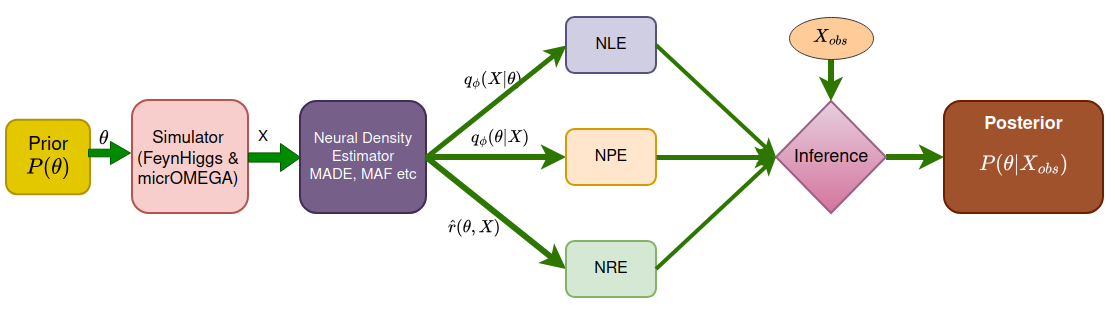
Figure 1: The flowchart of all the three SBI algorithms i.e., NPE, NLE and NRE is displayed in this figure.

2.1.1 Neural Posterior Estimation

In this approach, one directly trains to learn the posterior distribution $\mathcal{P}(\bm{\theta}|\bm{x})$ by optimizing the loss function defined as negative of the expectation value of $\log\hat{\mathcal{P}}(\bm{\theta}|\bm{x})$ in the training dataset papamakarios2018fastepsilonfreeinferencesimulation ; greenberg2019automatic i.e.,

$$\mathcal{L}_{\rm NPE} :=-\mathbb{E}_{\mathcal{D}_{\rm train}}\log\hat{\mathcal{P}}(\bm{\theta}|\bm{x})$$ (3)

$$=-\mathbb{E}_{\mathcal{D}_{\rm train}}\log\left[\frac{p(\bm{\theta})}{\tilde{p}(\bm{\theta})}q_{\phi}(\bm{\theta}|\bm{x})\right],$$

where $\hat{\mathcal{P}}(\bm{\theta}|\bm{x})$ is the product of a neural network output $q_{\phi}(\bm{\theta}|\bm{x})$ and a weighting factor taken as the ratio of the assumed prior $p(\bm{\theta})$ to the proposal prior $\tilde{p}(\bm{\theta})$. The proposal prior is defined as the distribution of $\bm{\theta}$ present in the training dataset $\mathcal{D}_{\rm train}$, while the assumed prior is an experimental design choice representing a priori knowledge of the global distribution of $\bm{\theta}$.

2.1.2 Neural Likelihood Estimation

NLE papamakarios2019neural uses neural networks to estimate the likelihood function by optimizing the loss function given by

$$\mathcal{L}_{\rm NLE}:=-\mathbb{E}_{\mathcal{D}_{\rm train}}\log q_{\phi}(\bm{x}|\bm{\theta}).$$ (4)

Once optimized over $\phi$, the trained $q_{\phi^{*}}(\bm{x}|\bm{\theta})$ can be multiplied with $p(\bm{\theta})$ to obtain $\hat{\mathcal{P}}(\bm{\theta}|\bm{x})$ i.e. $\hat{\mathcal{P}}(\bm{\theta}|\bm{x})\propto p(\bm{\theta})q_{\phi^{*}}(\bm{x}|\bm{\theta})$. One advantage of the NLE method over NPE (as is obvious from comparing equation 4 with 3) is that it does not require the knowledge of the analytical expression for $\tilde{p}(\bm{\theta})$. It is worth pointing out that in this method one calculates the likelihood for every parameter set only while preparing the dataset but not at the time of training or testing.

2.1.3 Neural Ratio Estimator

In this method, one first defines the likelihood ratio Hermans_2019

$$r(\bm{x},\bm{\theta})=\frac{\mathcal{P}\left(\bm{x}|\bm{\theta}\right)}{\mathcal{P}(\bm{x})}=\frac{\mathcal{P}(\bm{x},\bm{\theta})}{\mathcal{P}(\bm{x})\mathcal{P}(\bm{\theta})}=\frac{\mathcal{P}^{\rm joint}}{\mathcal{P}^{\rm marginal}}$$ (5)

In (cranmer2015approximating, ), the authors show that this equation “can be used in a supervised learning setting to train a binary classifier $d_{\phi}(\bm{x},\bm{\theta})$ to distinguish joint samples $\{\bm{x},\bm{\theta}\}\sim\mathcal{P}^{\rm joint}$ with class label $y=1$ from marginal samples $\{\bm{x},\bm{\theta}\}\sim\mathcal{P}^{\rm marginal}$ with class label $y=0$”. Once trained, the classifier can be written as

$$d_{\phi*}(\bm{x},\bm{\theta})=\frac{\mathcal{P}^{\rm joint}}{\mathcal{P}^{\rm joint}+\mathcal{P}^{\rm marginal}}$$ (6)

where the optimal parameters $\phi^{*}$ are obtained using an Adam optimizer kingma2014adam with binary cross-entropy loss of the form

$$\mathcal{L}_{\rm NRE}=-\int\left[\mathcal{P}^{\rm joint}\ln{d_{\phi}(\bm{x},\bm{\theta})}+\mathcal{P}^{\rm marginal}\ln\{1-d_{\phi}(\bm{x},\bm{\theta})\}\right]d\bm{\theta}d\bm{x}$$ (7)

As is obvious from the equations 5 and 6, the approximated ratio can then be obtained from

$$r(\bm{x},\bm{\theta})=\frac{d_{\phi^{*}}(\bm{x},\bm{\theta})}{1-d_{\phi^{*}}(\bm{x},\bm{\theta})}.$$ (8)

In this work, we use the well established and very successful classifier ResNET for estimating $r(\bm{x},\bm{\theta})$.

2.2 Choosing the right method

The general guidelines for choosing one method over another are the following:

• If the data is high-dimensional (e.g., in case of images) NPE may be a more viable choice than NLE or NRE.

• In some problems, the likelihood may be more straight-forward for neural learning than the posterior distribution. For such case, NLE is preferred over NPE or NRE.

• In case of NRE, one typically uses very well known neural-network architecture such as ResNET as mentioned above. It is a big advantage over NPE or NLE considering one has to spend a significant amount of time in choosing the suitable network for NPE and NLE.

However, in reality, for most of the cases, one has to try all three SBI methods and only then depending on the performance one chooses one method over another. Now we will discuss in more detail about the choice of estimator $q_{\phi}(\bm{x}|\bm{\theta})$. As emphasized earlier, the main aim of the neural network will be to obtain $q_{\phi}(\bm{x}|\bm{\theta})$ by varying $\phi$ such that $q_{\phi^{*}}(\bm{x}|\bm{\theta})\simeq p(\bm{x}|\bm{\theta})$. With great advancement in neural network architecture in the last few years, the de-facto choices for the estimator become neural density networks such as Masked Autoregressive Flow (MAF) (papamakarios2017masked, ), Mixture density networks (MDNs)(bishop1994mixture, ), and Neural Spline Flow (NSF) durkan2019neuralsplineflows .

In this work, we use MAF, which has demonstrated excellent performance across various general-purpose density estimation tasks. MAF starts from a base distribution, typically a Gaussian $\mathbf{z_{0}}\sim\mathcal{N}\mathopen{}\left(\mathbf{0},\mathbf{I}\right)\mathclose{}$ and applies a series of autoregressive functions $(f_{1},f_{2},...f_{k})$ to obtain the target distribution $\mathbf{z_{K}}$, Papamakarios_2018 i.e.,

$$\bm{x}=\mathbf{z_{K}}\quad\text{where}\quad\begin{array}[]{l}\mathbf{z}_{0}\sim\mathcal{N}\mathopen{}\left(\mathbf{0},\mathbf{I}\right)\mathclose{}\\ \mathbf{z}_{k}=f_{k}\mathopen{}\left(\mathbf{z}_{k-1},\mathbf{\bm{\theta}}\right)\mathclose{}.\\ \end{array}$$ (9)

Here, every $f_{k}$ is a bijection mapping implemented by Masked autoencoder for Distribution Estimation (MADE) germain2015made and is characterized by hyperparameters “Number of Hidden Layer” and “Number of Transformer”.

$$q^{\rm MAF}_{\phi}(\bm{x}|\bm{\theta})=\mathcal{N}\mathopen{}\left(\mathbf{z}_{0}\,|\,\mathbf{0},\mathbf{I}\right)\mathclose{}\prod_{k}{\absolutevalue{\det\mathopen{}\left(\frac{\partial{f_{k}}}{\partial{\mathbf{z}_{k-1}}}\right)\mathclose{}}^{-1}}$$ (10)

The learnable parameters $\phi$ can then be obtained by optimizing the loss function

$$\mathcal{L}_{\rm MAF}:=-\mathbb{E}_{\mathcal{D}_{\rm train}}\left[\log q^{\rm MAF}_{\phi}(\bm{x}|\bm{\theta})\right],$$ (11)

where the expectation $\mathbb{E}_{\mathcal{D}_{\rm train}}$ is taken over all data-parameter pairs in the training set $\mathcal{D}_{\rm train}$. Once optimized, $q_{\phi}^{\rm MAF}$ approaches the true likelihood function $\mathcal{P}\left(\bm{x}|\bm{\theta}\right)$.

2.2.1 Testing the validity of the SBI methods - TARP

The aim of any validation method for SBI is to quantitatively determine the accuracy of the estimated posterior distribution $\hat{\mathcal{P}}(\bm{\theta}|\bm{x})$ compared to the true posterior distribution $\mathcal{P}(\bm{\theta}|\bm{x})$. Very recently, the authors in Ref. 2023PMLR..20219256L have proposed the TARP method to validate different SBI methods. The authors argued that this approach is necessary and sufficient to show that a posterior estimator is accurate. They also showed that this can detect inaccurate inferences in cases where other existing methods fail. Described below is the step-by-step procedure for the TARP test.

1. One first separates the test dataset pair $\mathcal{D}_{\rm test}=\left\{\bm{\theta}^{i}_{\rm test},\bm{x}^{i}_{\rm test}\right\}^{i=N_{\rm test}}_{i=1}$ from the train data set $\mathcal{D}_{\rm train}$. We make sure that the test dataset has never been used while training.

2. Take a test point $\bm{x}^{i}_{\rm test}$, choose a random reference point $(\bm{\theta}^{i}_{r})$ from a Uniform distribution in the range $[0,1]$.

3. Draw $N_{\rm p}$ points from the estimated posterior distribution $\hat{\mathcal{P}}(\bm{\theta}|\bm{x})$ i.e.,
   $\{\bm{\theta}^{i,p}_{\rm predicted}\}^{p=N_{\rm p}}_{p=1}\sim\hat{\mathcal{P}}(\bm{\theta}|\bm{x}^{i}_{\rm test})$.

4. Next we calculate the euclidean distance between the reference point $\bm{\theta}^{i}_{r}$ and $\bm{\theta}^{i,p}_{\rm predicted}$ and denote this set by $\left\{d(\bm{\theta}^{i,p}_{\rm predicted},\bm{\theta}^{i}_{r})\right\}^{p=N_{p}}_{p=1}$.

5. We also calculate distance $d(\bm{\theta}^{i}_{\rm test},\bm{\theta}^{i}_{r})$ between true parameter ($\bm{\theta}^{i}_{\rm test}$) and the reference point.

6. Compute the fraction of the points $\left\{d(\bm{\theta}^{i,p}_{\rm predicted},\bm{\theta}^{i}_{r})\right\}^{p=N_{\rm p}}_{p=1}$ with distance smaller than $d(\bm{\theta}^{i}_{\rm test}.\bm{\theta}^{i}_{r})$. This fraction is called the credibility level defined as $1-\alpha$, where $\alpha$ is the confidence level. The higher the fraction, better is the estimate.

7. Steps 2-6 are repeated for all the $N_{\rm test}$ points in the test dataset.

8. Once the credibility level is determined for all the test data pairs, we then compute the histogram describing the coverage distribution of $\alpha$. The cumulative distribution of $\alpha$ multiplied with the bin width of the histogram is called the Expected Coverage Probability (ECP). For an accurate posterior estimator, $\rm ECP=1-\alpha$, i,e, a straight line with $45^{0}$ inclination with the x-axis where x and y-axis represent the credibility level and expected coverage, respectively.

In summary, the credibility level refers to the probability threshold used to define the credible interval or confidence level, indicating the degree of belief that the true parameter lies within this interval. On the other hand, the expected coverage is the number of times the true parameter value is actually contained within the credible intervals when averaged over many independent samples. We show the TARP test result in Section. 4.2.

3 Analysis set-up in pMSSM

In this study, we analyze the pMSSM framework, detailing the parameters and their possible ranges within the model. We discuss constraints on sparticle masses imposed by LHC searches to date and identify the currently allowed parameter space for further exploration. The focus is primarily on the scalar sector, along with other key observables, such as flavor decay branching ratios. The scalar sector of pMSSM consists of two ${\rm SU(2)_{L}}$ doublets that result in two neutral CP even, one neutral CP-odd, and one charged Higgs states. Among the two CP-even states, the lighter one can be interpreted as the SM-like Higgs. Given the precise measurements of the corresponding mass and coupling strengths, it cannot have large mixing with the other CP-even state. One can use this to constrain the scalar sector parameters such as $M_{A}$, $\mu$, $\tan\beta$, and $A_{t}$. We take this approach coupled with direct search constraints of SUSY particles and flavor constraints for our analysis. Finally, we outline the preparation of the sample containing parameters with corresponding observables and present the results of our analysis.

3.1 Constraints on SUSY particles from collider searches

Both the ATLAS and CMS Collaborations have conducted extensive searches for SUSY over the years. These searches cover a wide range of final states, looking for evidence of sparticles. Some key final states explored include jets + missing transverse energy (MET), leptons + jets + MET, multilepton final states, photons + MET, $b$-tagged jets + MET, and long-lived particles, etc. ATLAS and CMS have excluded gluino masses up to $\sim$ 2.0-2.3 TeV from various final states for lightest supersymmetric particle (LSP) $\widetilde{\chi}_{1}^{0}$ masses up to 600 GeV CMS:2019zmd ; ATLAS:2020syg ; ATLAS:2021twp ; CMS:2021beq ; CMS:2019ybf ; CMS:2020cpy ; CMS:2022idi ; CMS:2020bfa . Similarly light squarks are also limited upto 1.25-1.85 TeV for a massless LSP CMS:2019zmd ; ATLAS:2020syg ; ATLAS:2021twp ; CMS:2021beq ; ATLAS:2023afl ; ATLAS:2022zwa . Additionally, sleptons are excluded up to 700 GeV ATLAS:2019lff ; CMS:2020bfa , wino-like chargino and second lightest neutralino upto $\sim$ 900-1450 GeV ATLAS:2022zwa ; ATLAS:2021yqv ; CMS:2021cox ; CMS:2022sfi , higgsino-like charginos and heavy neutralinos upto 800 GeV CMS:2022sfi ; CMS:2024gyw , assuming a massless bino type neutralino. However, it is worth mentioning that if the LSP mass is above 500 GeV, there is no limit on wino-like chargino or sleptons. Pure higgsino-like chargino-neutralinos are also excluded upto 205-210 GeV CMS:2021edw ; ATLAS:2021moa . The long-lived charginos are also searched at the LHC and are excluded up to 610-884 GeV GeV ATLAS:2022rme ; CMS:2020atg depending upon the lifetime. While performing the analysis, we maintain all these collider limits on sparticles.

3.2 Observables

As we have mentioned above that we mainly focus on the Higgs sector for our analysis. The discovery of the Higgs boson in 2012 by the ATLAS and CMS experiments at the LHC was a monumental achievement in particle physics, confirming the last missing piece of the Standard Model (SM). However, this discovery also opens the door to exploring Beyond the Standard Model (BSM) physics. We know that pMSSM can easily stabilize the Higgs mass against quantum corrections MSSMWorkingGroup:1998fiq ; Allanach:2004rh . The tree-level Higgs mass depends on $\tan\beta$, the ratio of two vacuum expectation values (vev), and $M_{A}$, the mass of pseudoscalar Higgs. But there is a radiative correction to the tree level mass and this correction depends on many other pMSSM parameters like $A_{t}$, $\mu$, and soft SUSY breaking parameters. The Higgs decays also have QCD and electroweak corrections which depend on various SUSY parameters. Here we consider different observables like Higgs mass $m_{h}$, Higgs coupling strength for both the production mode ($\mu_{i}$) and decay channel ($\mu^{f}$), and the branching ratios of $B$-hadron decays. From the combined results provided by ATLAS and CMS analyses, we know that the SM-like Higgs boson mass is 125.09$\pm$0.21(stat.)$\pm$0.11(syst.) GeV CMS:2012qbp ; ATLAS:2012yve ; ATLAS:2015yey . But we know that there are theoretical uncertainties in the SUSY framework  Allanach:2004rh and due to that we consider Higgs mass as $125\pm 1$ GeV. The signal strength for a production mode $i$ and a particular decay channel $f$ is defined as $\mu_{i}=\frac{\sigma_{i}}{(\sigma_{i})_{SM}}$ and $\mu^{f}=\frac{\mathcal{B}^{f}}{(\mathcal{B}^{f})_{SM}}$ respectively. Both the experiments, ATLAS and CMS have provided these $\mu_{i}$ and $\mu_{f}$ values. We consider the values provided by CMS collaboration CMS:2020gsy . We also consider three different flavor physics observables such as $\mathcal{B}r(B\rightarrow X_{s}\gamma)$ HFLAV:2019otj , $\mathcal{B}r(B_{s}\rightarrow\mu^{+}\mu^{-})$ LHCb:2021vsc and $\frac{\mathcal{B}r(B\rightarrow\tau\nu)}{\mathcal{B}r(B\rightarrow\tau\nu)_{SM}}$ Belle:2010xzn ; Belle:2014eud ; Belle:2015odw . The best-fit and $1\sigma$ values of all these observables are mentioned in the Table. 1.

Observable	Best-fit $\pm~1\sigma$	Observable	Best-fit $\pm~1\sigma$
$m_{h}$ (GeV)	$125\pm 1.0$	$\mu_{WH}$	1.46${}^{+0.37}_{-0.35}$
$\mathcal{B}r(B\rightarrow X_{s}\gamma)$	(3.32 $\pm$ 0.15)$\times 10^{-4}$	$\mu_{ZH}$	0.98${}^{+0.31}_{-0.30}$
$\mathcal{B}r(B_{s}\rightarrow\mu^{+}\mu^{-})$	(3.09${}^{+0.46+0.15}_{-0.43-0.11}$)$\times 10^{-9}$	$\mu^{ZZ}$	0.93${}^{+0.10}_{-0.09}$
$\frac{\mathcal{B}r(B\rightarrow\tau\nu)}{\mathcal{B}r(B\rightarrow\tau\nu)_{SM}}$	1.28 $\pm$ 0.25	$\mu^{WW}$	1.20${}^{+0.16}_{-0.15}$
$\mu_{ggH}$	1.04 $\pm$ 0.09	$\mu^{bb}$	1.11${}^{+0.20}_{-0.19}$
$\mu_{VBF}$	0.75${}^{+0.19}_{-0.17}$	$\mu^{\tau\tau}$	0.80${}^{+0.17}_{-0.16}$
$\mu_{ttH}$	1.14${}^{+0.21}_{-0.20}$	$\mu^{\gamma\gamma}$	1.07${}^{+0.12}_{-0.10}$

Table 1: The best-fit along with $1\sigma$ value of fourteen observables considered in our analysis are mentioned here.

3.3 Parameter space

There are 19 free parameters in pMSSM, and not all of them have a direct or significant effect on the Higgs sector and flavor observables. For our analysis, we vary a few of these parameters, which are most relevant while keeping others fixed at values decoupled from the rest. While we fix the parameters, we keep in mind the limits on sparticle masses coming from collider searches which are already discussed in Section. 3.1. To avoid the limits on squarks and sleptons, we decouple all the gluino, squark, and slepton masses by keeping them at 4 TeV. As we have mentioned for the LSP masses above 500 GeV, there is no limit on chargino-neutralino masses, we fix the LSP ($\widetilde{\chi}_{1}^{0}$) mass at 500 GeV. After that, we are left with wino mass parameter ($M_{2}$), Higgsino mass parameter ($\mu$), ratio of two vev ($\tan\beta$), pseudoscalar Higgs mass ($M_{A}$) and trilinear top coupling ($A_{t}$). The ranges of parameters used for the scanning are mentioned in the Table. 2. We have also done a separate analysis for the nine dimensional pMSSM parameter space by additionally varying bino, gluino, squarks, sleptons mass parameters, which is discussed in the Appendix. A.

Parameter	Range
$M_{2}$	550-5000
$\mu$	550-5000
$\tan\beta$	1-60
$M_{A}$	100-5000
$|A_{t}|$	0-8000

Table 2: Range of five free parameters considered for our analysis. All the parameters mentioned here have unit GeV except $\tan\beta$.

3.4 Sample preparation for SBI

To sample the parameter space, we use the FeynHiggs Heinemeyer:1998yj ; Heinemeyer:1998np ; Bahl:2016brp ; Bahl:2018qog package, and for calculating the branching ratios of $B$-hadron decays, we employ the micrOMEGAs Belanger:2004yn ; Belanger:2008sj ; Belanger:2010gh ; Belanger:2013oya ; Belanger:2020gnr . We initially perform a random scan of the entire parameter space to generate a sample file. This sample can be used for training purposes. However, to improve the efficiency of the prepared sample, we retain only those points that are consistent with all observables within the 3$\sigma$ limit of their best-fit values, as listed in Table 1. We generated approximately $6.0\times 10^{5}$ samples randomly, of which only around $2\times 10^{5}$ samples remain after applying the constraints. As mentioned above, we calculate the observables value corresponding to each parameter set using FeynHiggs and micrOMEGAs. To generate $6.0\times 10^{5}$ number of samples through those packages running parallel in 4 cores, it requires $\sim$ 22 hours of time .

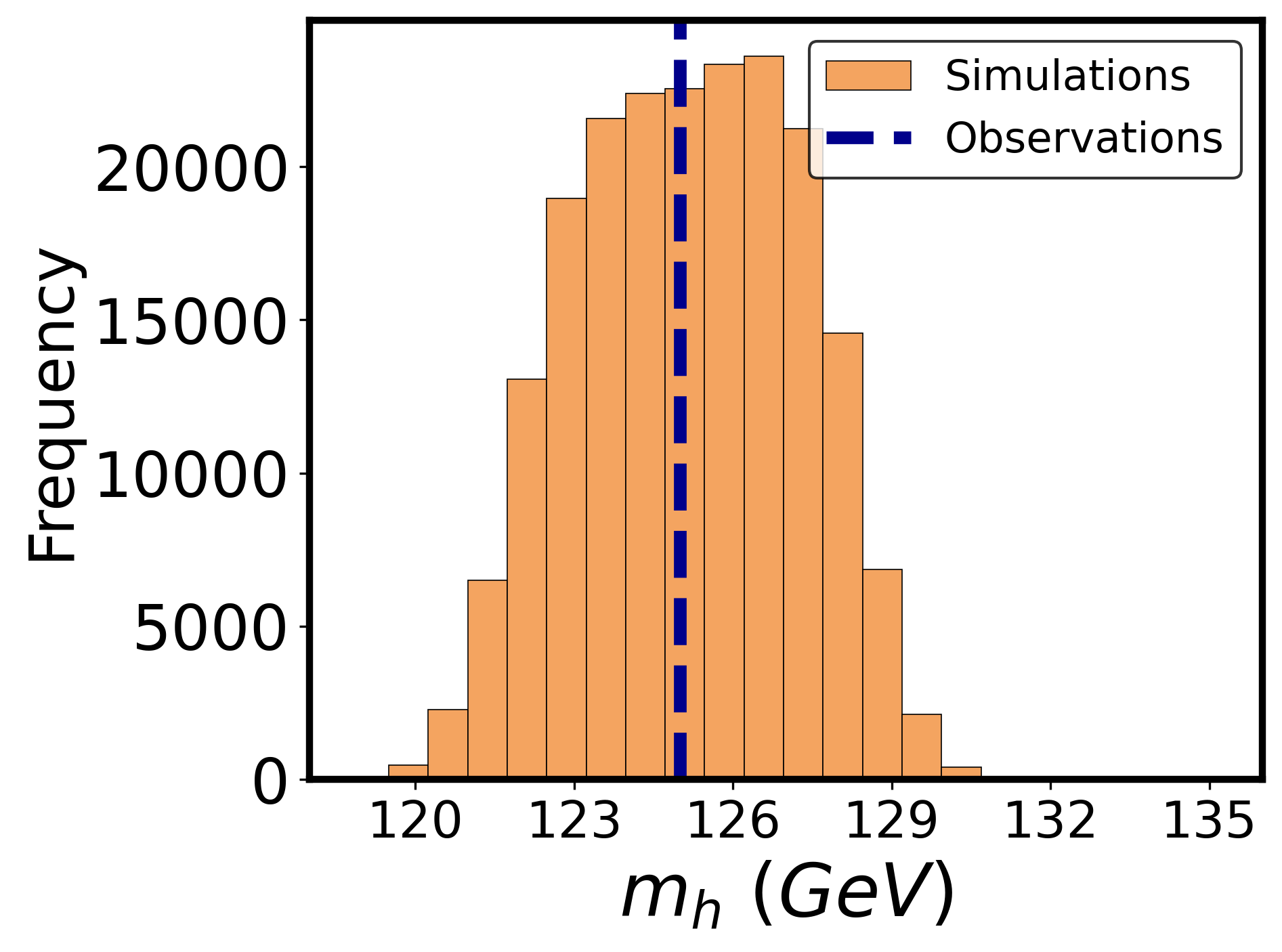
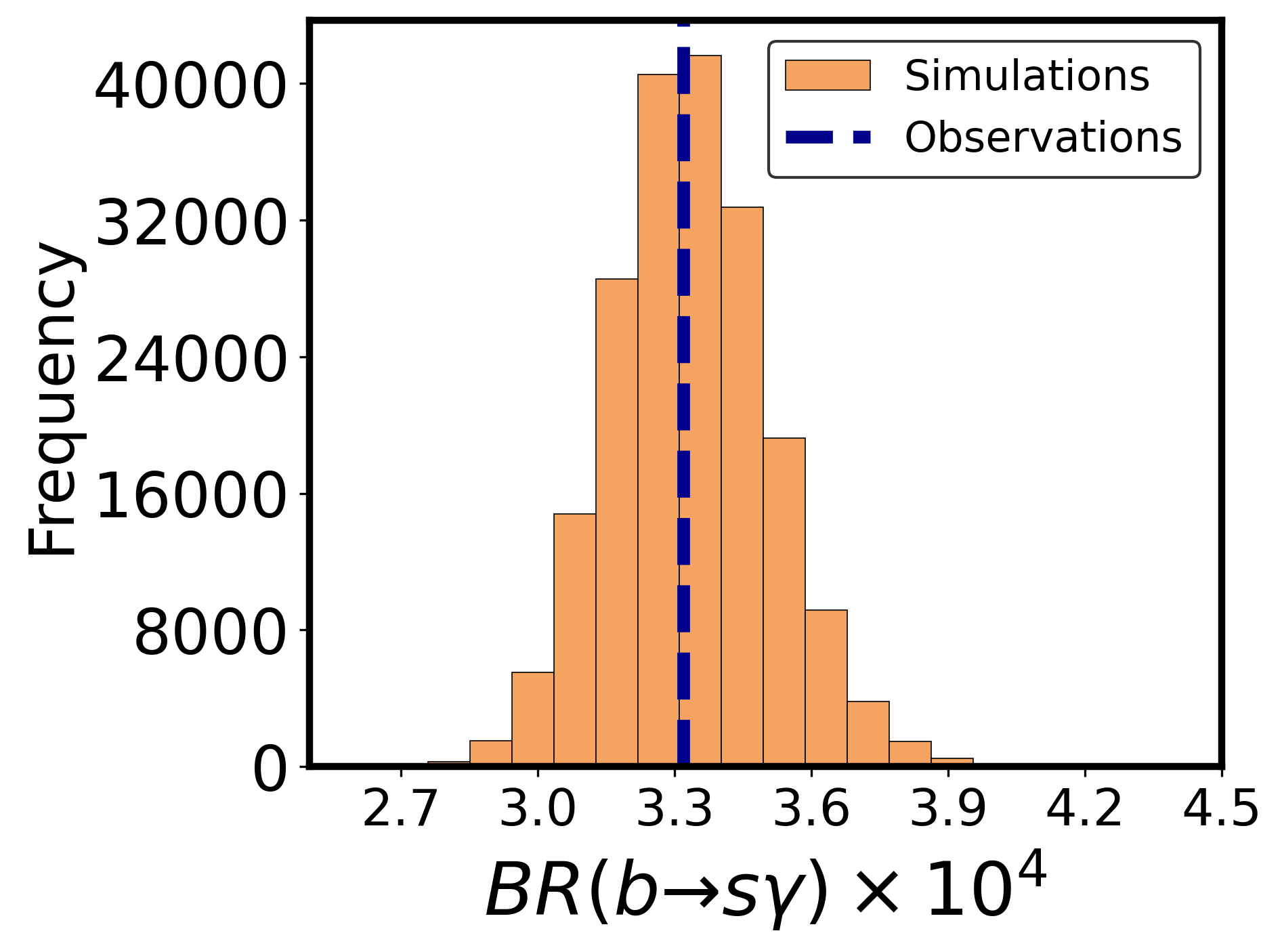
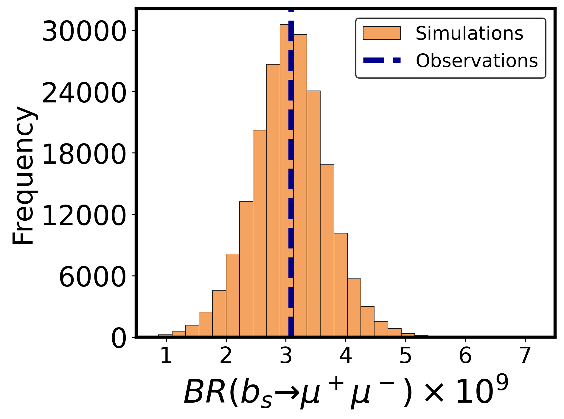
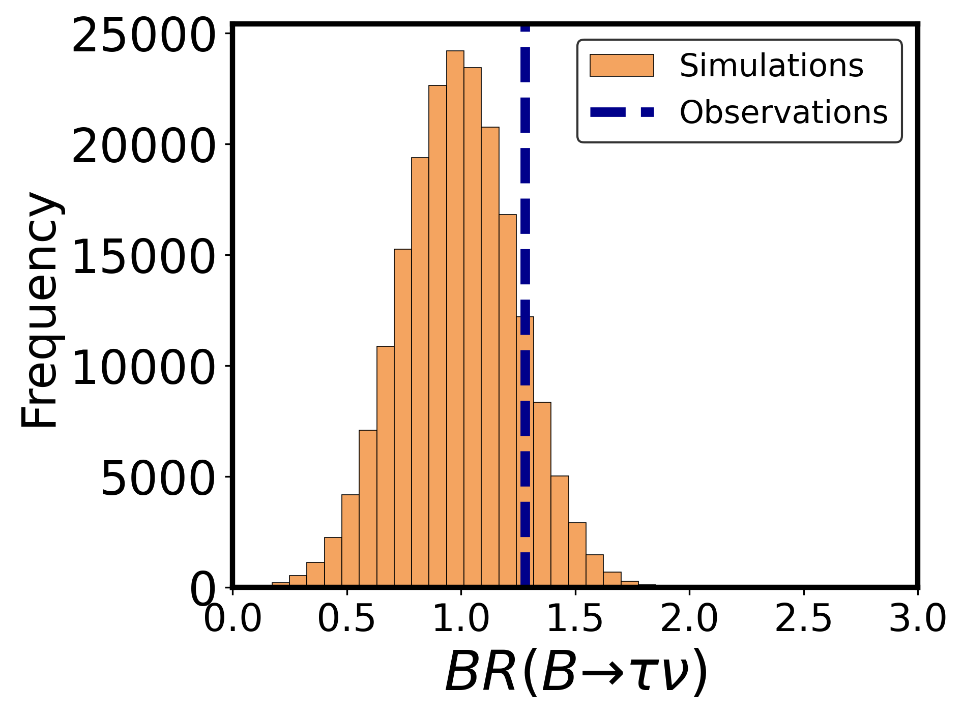
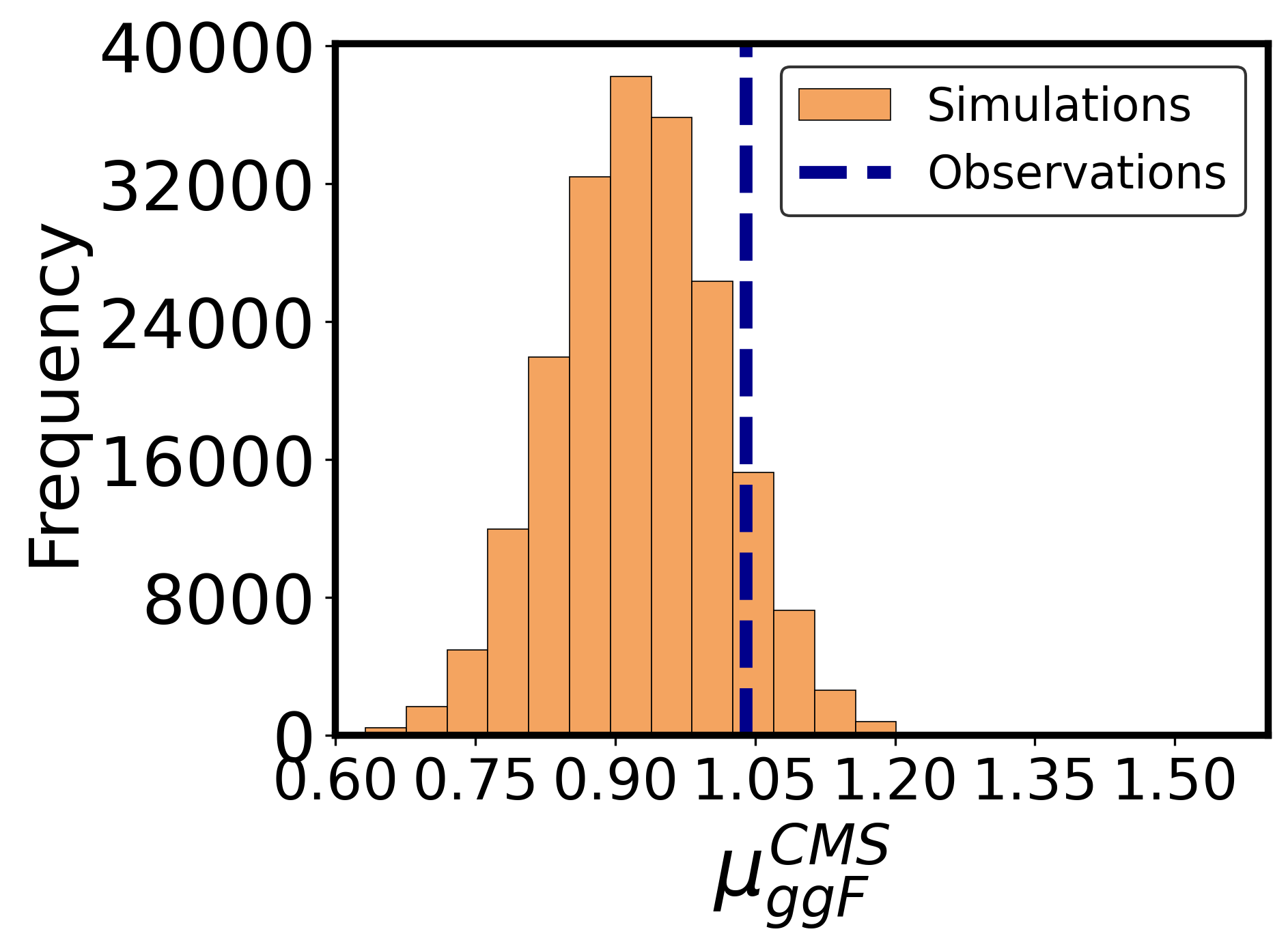
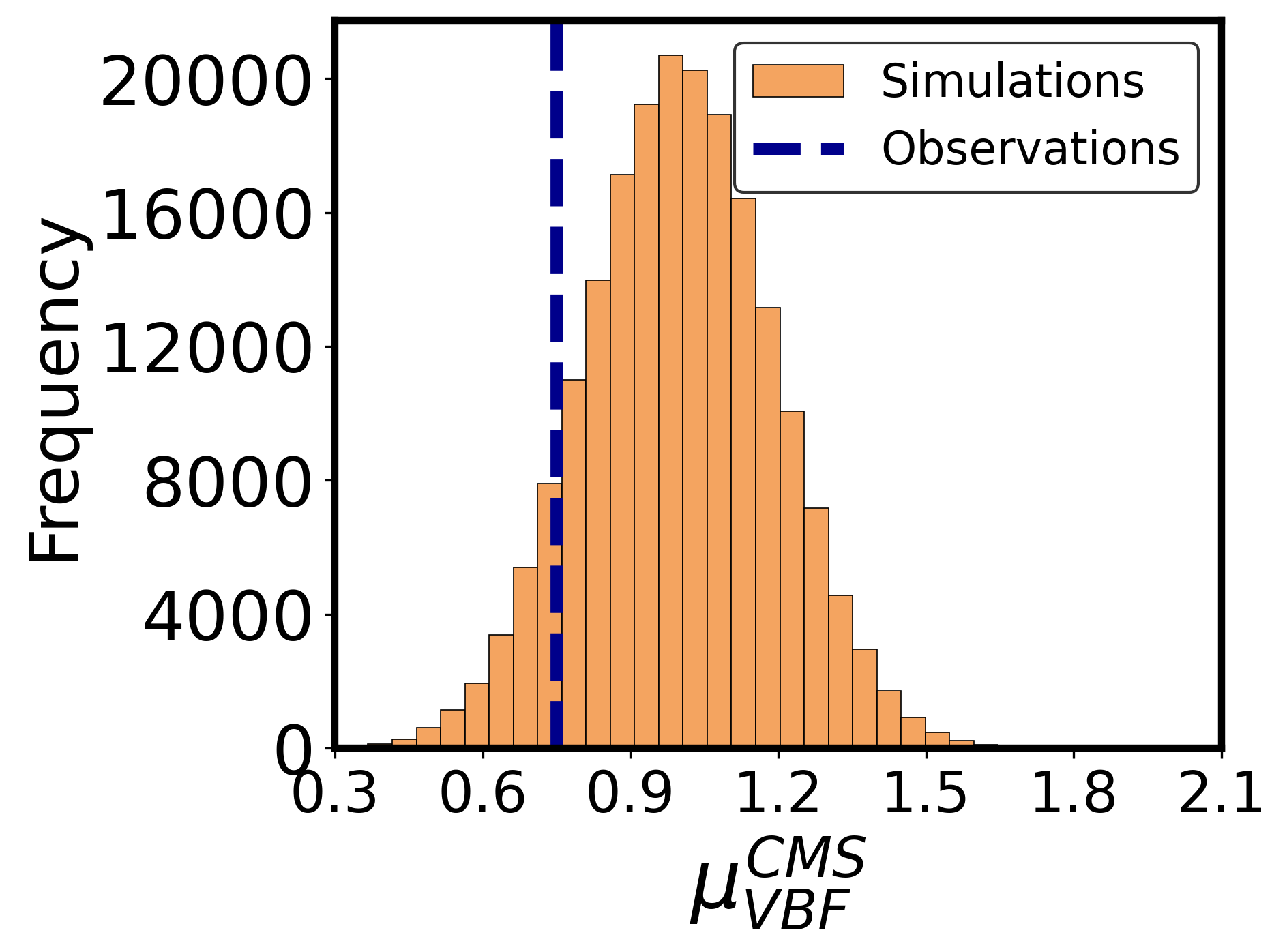
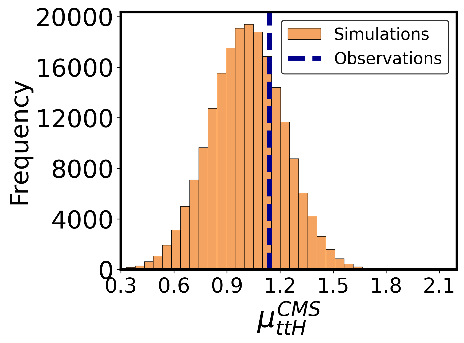
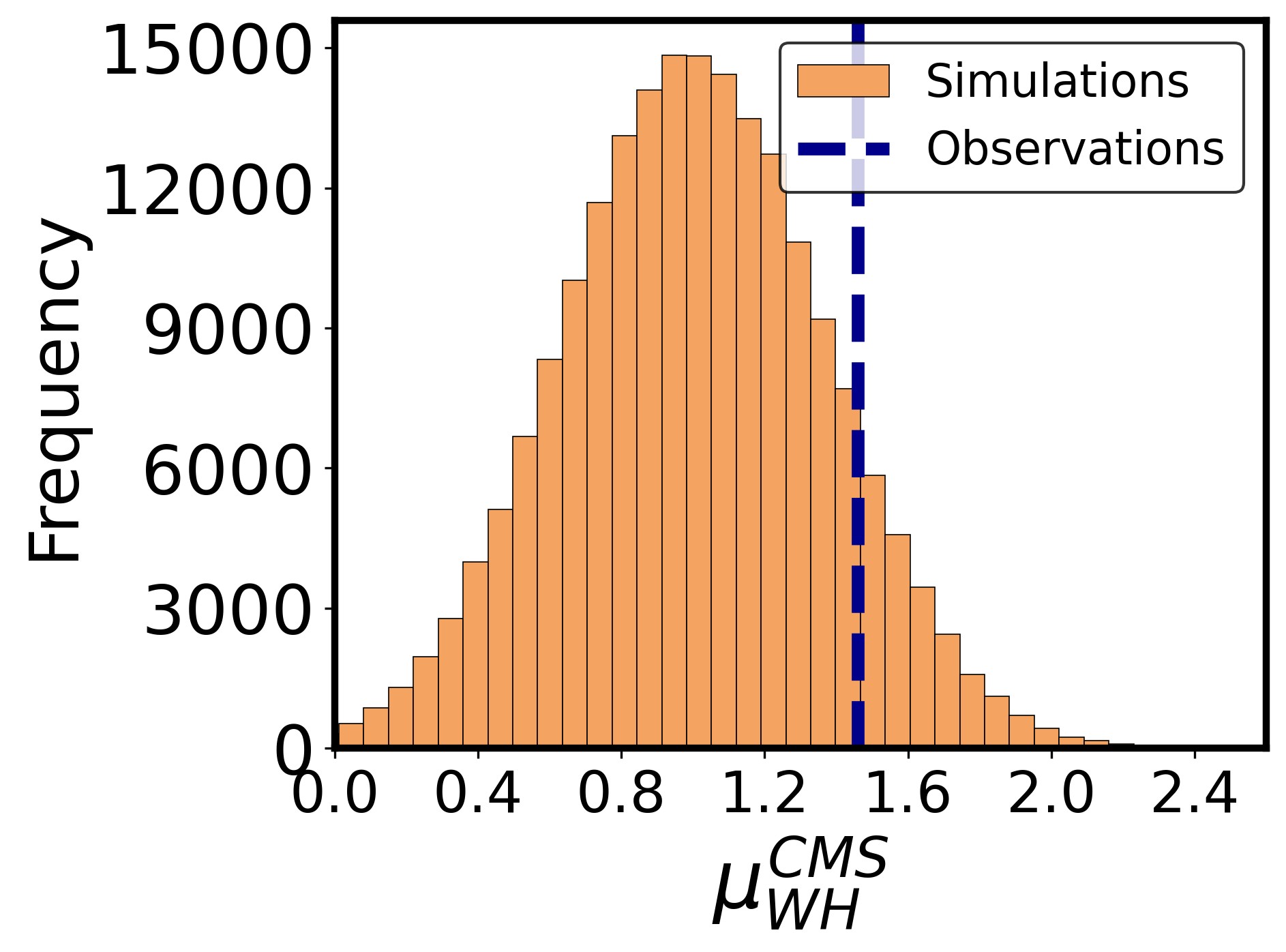
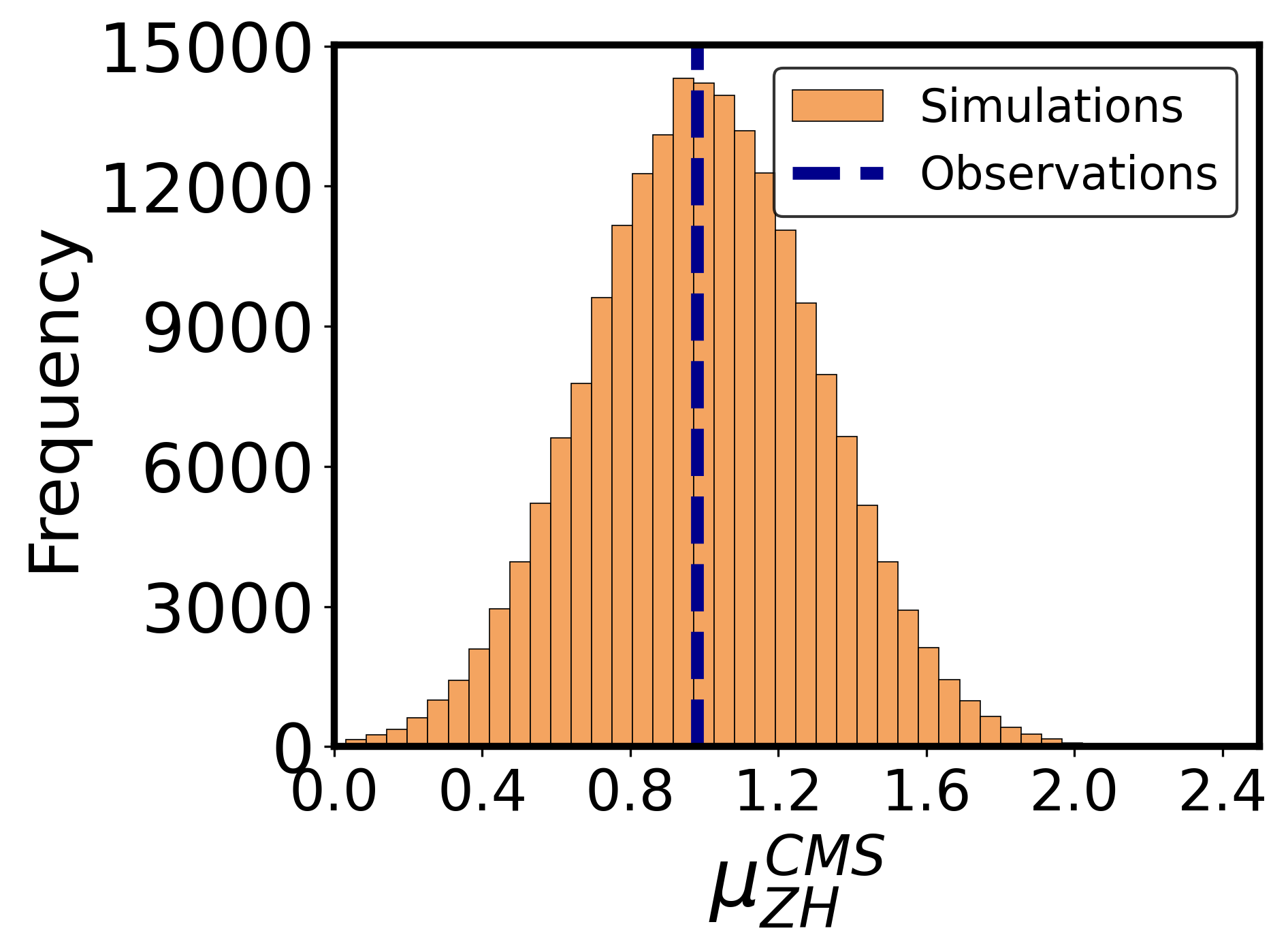
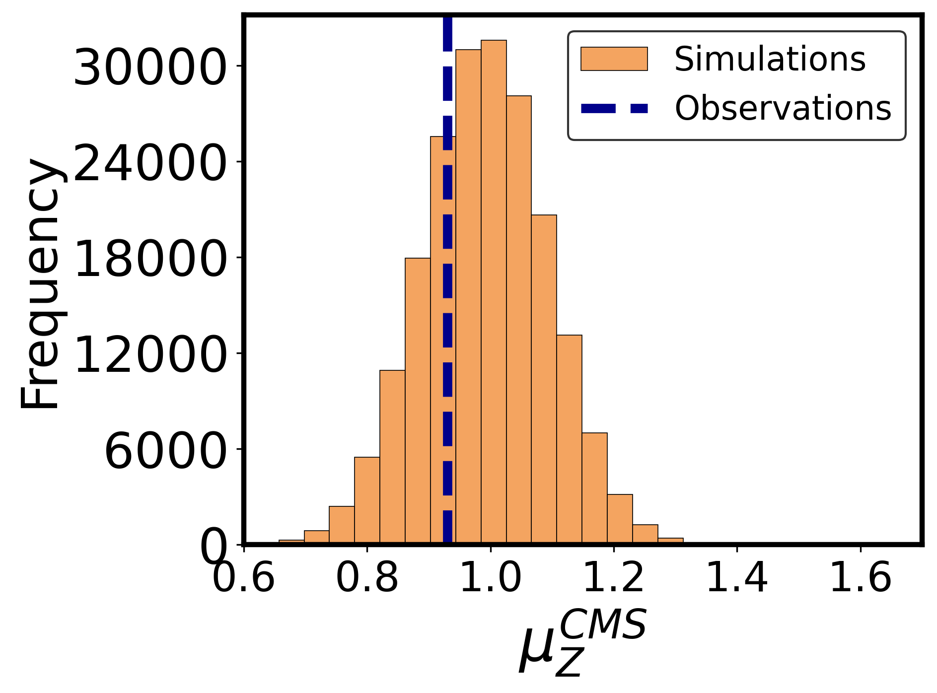
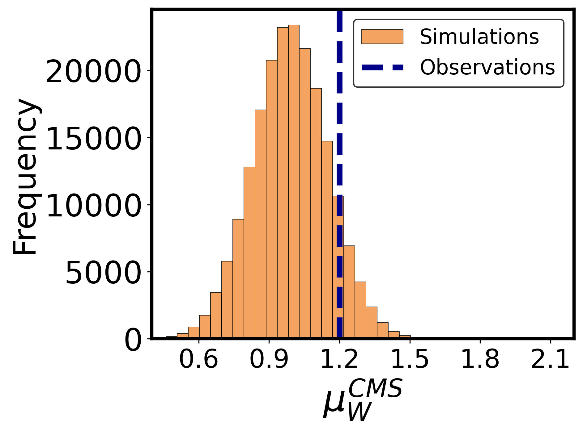
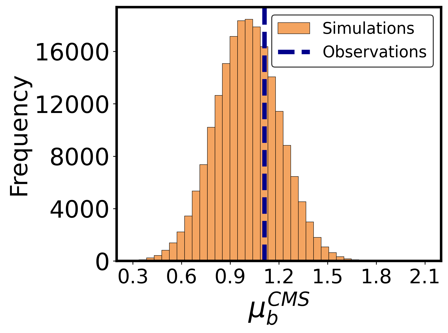
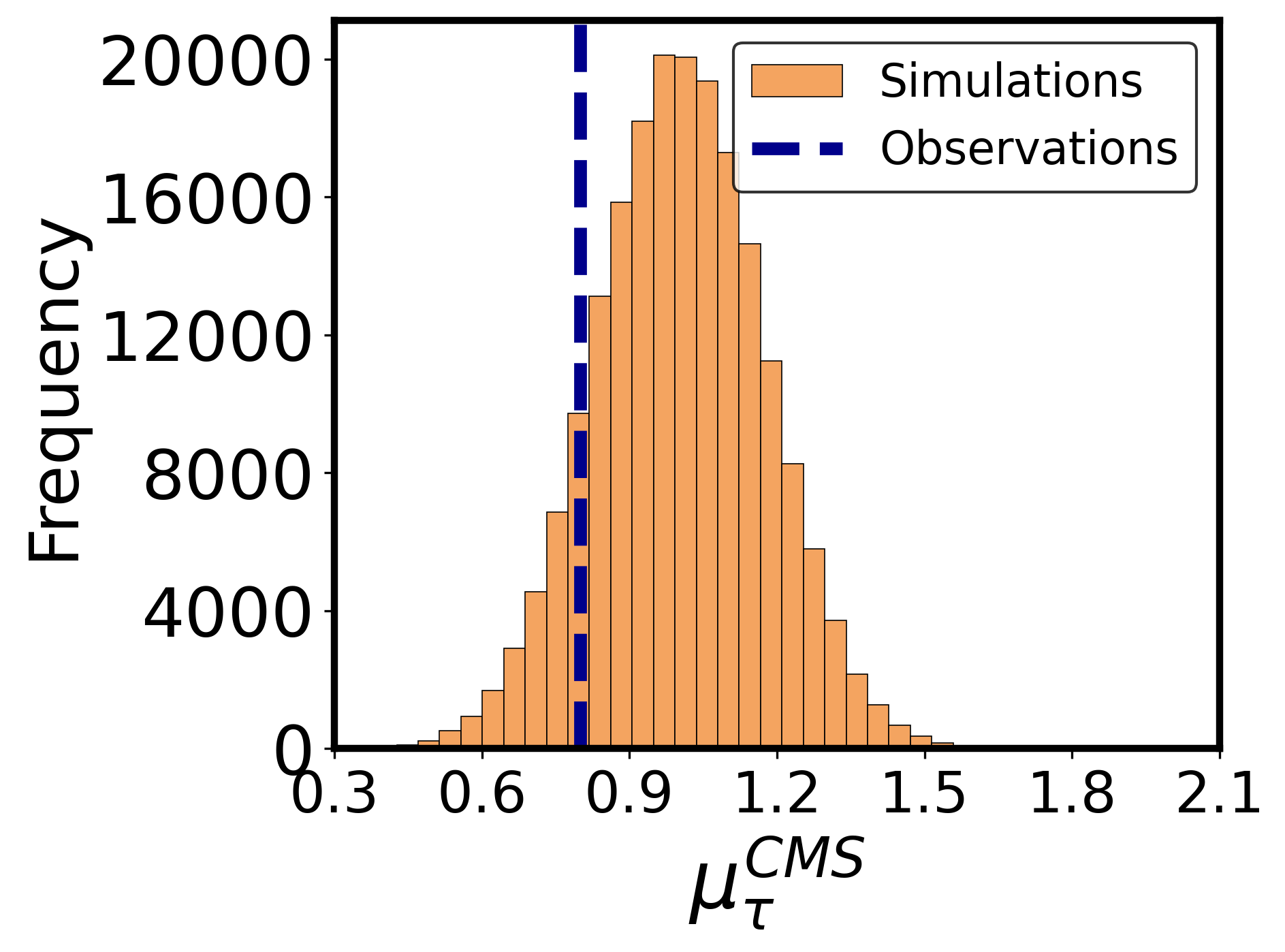
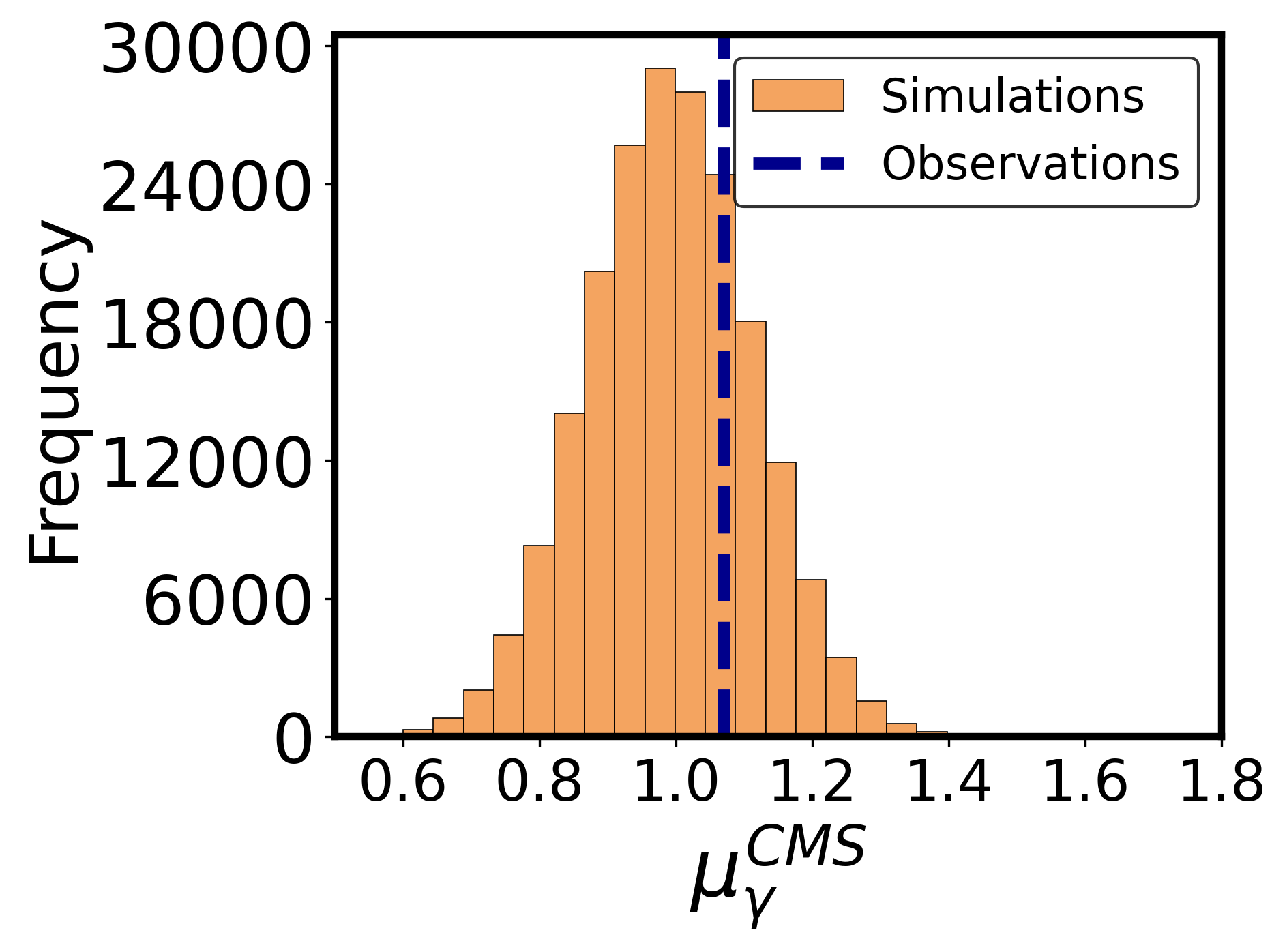
Figure 2: Distributions of all the 14 observables in training sample after adding the noise are displayed. The orange-brown histograms represent the simulated training sample distribution whereas the dashed blue lines indicate the true value of each observable.

To make the observables, calculated by FeynHiggs, resemble the experimental data, we need to add some noise or error ($\epsilon$) to the observables in the form $\mathcal{N}(0,\sigma^{2})$, where the $\sigma$ corresponding to each observables are already mentioned in the Table. 1. So, the observable, $f(x)$, generated by the packages will be updated to $f^{\prime}(x)=f(x)+\epsilon$. The training sample must be centered around the true values, as required by the SBI methods sbilink . To verify this, we plot the histogram of each observable after adding noise, as shown in Figure 2. The plot indicates that not all distributions are centered precisely around the true values. However, it is noteworthy that the true values, represented by the dashed dark blue lines, lie within the distribution of simulated observables, depicted by the light orange-brown histogram. Parameters often have different scales and ranges, which can bias the model or lead to numerical instability, such as overflow or underflow during computation. Normalizing parameters to the range [0, 1] ensures a stable and balanced learning process. Once the posterior samples are drawn, we denormalize them to retrieve the parameters in their original scale for meaningful interpretation.

4 LtU-ILI framework for pMSSM

We now describe the implementation of the SBI method for the pMSSM model using publicly available LtU-ILI (Learning the Universe Implicit Likelihood Inference) code 2024OJAp….7E..54H . This package trains neural network based SBI models for estimating posterior distributions of the model parameters. Additionally, the LtU-ILI code offers a variety of tools that users can utilize for testing and validating the trained models. We refer the interested readers to follow the Ref. 2024OJAp….7E..54H for more details.

We first determine the minimum number of samples required to accurately reconstruct the posterior of the model parameters. For that, we gradually increase the number of samples ($10^{3}$, $2\times 10^{3}$, $5\times 10^{3}$ …) in the training dataset from our previously stored $2\times 10^{5}$ samples (as mentioned in Section 3.4). For each case, 95% of the samples are allocated for training, and 5% are reserved for validation of the SBI model using the TARP test. After training, posterior samples are drawn around the central values of each observable. To measure the posterior sample efficiency, we input the posterior samples into the FeynHiggs package to calculate the corresponding observables. For each parameter set, we check whether the observables lie within $3\sigma$ of the values specified in Table 1. The posterior sample efficiency is defined as the ratio of parameter sets meeting the $3\sigma$ condition to the total number of posterior samples generated. We also compare the time consumption of each algorithm corresponding to different sample subsets.

4.1 Ablation study and hyperparameter set-up

Since each SBI method uses a neural network with distinct architectures and features, we now carry out an ablation study to find out the best set of hyperparameters. In both NPE and NLE methods, we use MAF “density_estimator”, whereas for NRE, we use ResNET, as already mentioned in Sections  2.2 and  2.1.3. There are different hyperparameters for MAF density function such as “hidden_features” (HF) and “num_transforms” (NT) along with other ML hyperparameters like “Training Batch size” (TBS), “Learning rate” (LR) etc.

Fixed Part		Efficiency with varying hyperparameter
MAF 1 layer	HF value	2	10	50	100	400	600	800	1000
NT=20, TBS=512
LR=$0.0001$	Efficiency (%)	96.67	97.29	98.70	99.34	99.51	98.88	97.68	96.88
MAF 1 layer	NT value	1	2	5	10	20	40	70	100
HF=400, TBS=512
LR=$0.0001$	Efficiency (%)	96.4	97.10	97.80	98.88	99.51	99.56	99.60	99.62
MAF 1 layer	TBS value	16	32	64	128	256	512	1024	2048
HF=400, NT=20
LR=$0.0001$	Efficiency (%)	98.09	98.87	99.16	99.27	99.45	99.51	98.96	97.60
MAF 1 layer	LR value	0.00001	0.0001	0.001	0.01	0.1	0.3	0.5	1.0
HF=400, NT=20
TBS=512	Efficiency (%)	98.68	99.51	99.56	99.27	99.05	98.78	98.06	97.60
HF=400, NT=20	MAF layer	1		2		3		4
TBS=512, LR=0.0001	Efficiency (%)	99.51		99.32		99.02		99.60

Table 3: The effect of hyperparameter variation on posterior sample efficiency is illustrated for the NPE algorithm with $10^{5}$ samples.

In LtU-ILI, one can define nets by using multiple layers of the same or different density estimators/functions, which have their own features that can be adjusted to analyze their impact on the posterior sample efficiency. Ideally, one should perform the hyperparameter optimization by varying all the elements of the networks simultaneously. However, due to limited computational resources, we restrict ourselves to an ablation study where we only vary certain parts of the network while keeping the rest at some fixed values. The ablation study results for NPE algorithm are presented in Table. 3.

From the ablation study in Table 3, it is evident that the efficiency decreases both for very low and high values of the HF parameter. The efficiency reaches its maximum around HF = 400 when other parameters are fixed at the values specified in the table. A similar trend is observed for the TBS parameter. On the other hand, the efficiency consistently increases with larger NT values. However, it is worth pointing out that the improvement saturates after a certain threshold (NT = 20). We conducted a similar study for the NLE and NRE algorithms. However, as shown in Section 4.3, NPE yields the more promising results compared to others. Therefore, we have not discussed their ablation study in detail. The optimized hyperparameters considered for each algorithm, along with their values, are listed in Table 4.

Features	NPE	NLE	NRE
Density function	MAF	MAF	ResNET
used (1 layer)
Density function	“hidden_features”=400	“hidden_features”=200	“hidden_features”=200
features	“num_transforms”=20	“num_transforms”=20	“num_blocks”=20
Common hyperparameters
Batch size = 512, Learning rate = $10^{-4}$

Table 4: The density function along with the details of optimized hyperparameter are shown here for each algorithm

4.2 TARP test results

In this section, we discuss the TARP test results in detail. Figure 3 illustrates the TARP plot for various subsets corresponding to the NPE algorithm. It is important to note that TARP test results are presented only for subsets with more than $5\times 10^{3}$ samples, as smaller subsets tend to yield less meaningful or unreliable outcomes.

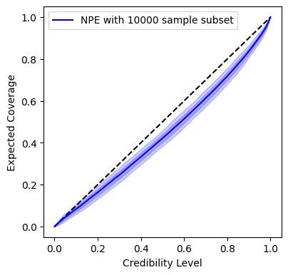
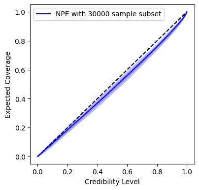
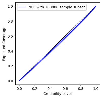
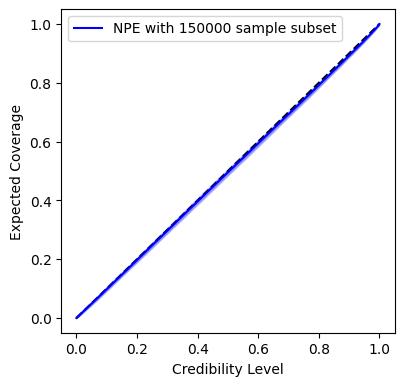
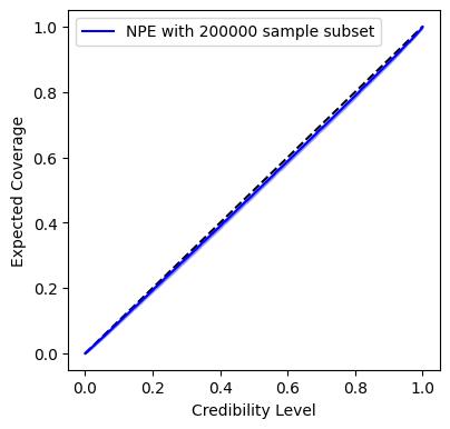
Figure 3: TARP test plot corresponding to $10^{4}$, $3\times 10^{4}$, $5\times 10^{4}$, $10^{5}$, $1.5\times 10^{5}$, $2\times 10^{5}$ sample subsets with NPE method are displayed here.

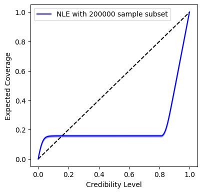
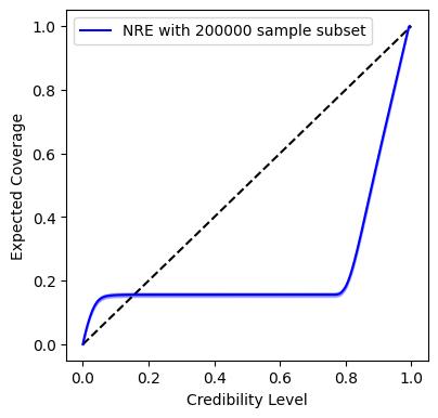
Figure 4: TARP test plot corresponding to $2\times 10^{5}$ sample subset for NLE (Left) and NRE (right) method are displayed here.

From Figure 3, it is clear that there is no significant improvement in the TARP plot beyond the $10^{5}$ sample subset for our model. Additionally, Figure 4 presents the TARP test results for the other two algorithms, focusing solely on the $2\times 10^{5}$ sample set. As is evident from the figure, neither of these two algorithms performs satisfactorily in the TARP test. It is also noteworthy that similar outcomes were observed for other sample subsets with these algorithms.

Based on the TARP test results, we conclude that the NPE algorithm demonstrates superior performance for the pMSSM model under consideration. This trend will be further corroborated by additional results, including posterior sample efficiency and time consumption.

4.3 Posterior sample efficiency and time consumption

As mentioned in Section. 3, we are interested in finding the posterior efficiency of model parameters, defined as

$$\text{Posterior efficiency}=\frac{\text{No of surviving samples within }3\sigma\text{ range of observable}}{\text{Total number of posterior samples drawn}}$$ (12)

Figure 5 shows the posterior sample efficiency (left panel) and time consumption (right panel) for each SBI method. In both panels, the blue (solid), red (dashed), and green (dot-dashed) lines correspond to the NPE, NLE, and NRE methods, respectively.

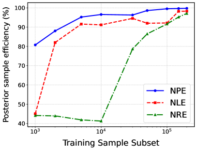
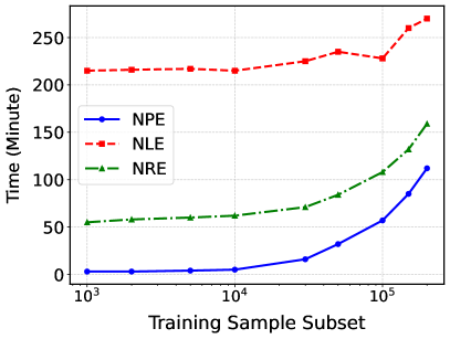
Figure 5: The comparison of posterior sample efficiency (left) and the time taken for different sample subsets corresponding to three different algorithms are displayed here.

From the left panel of the figure, we observe that posterior efficiency is not always directly proportional to the number of samples as also noted in Ref. Morrison:2022vqe . Notably, the NPE algorithm achieves higher posterior sample efficiency compared to NLE and NRE. Furthermore, the posterior sample efficiency for the NPE algorithm saturates after $10^{5}$ samples, whereas the NLE and NRE algorithms do not exhibit such behavior. To reach the desired posterior efficiency in our model, NPE requires only 50% of the total sample set, whereas NLE and NRE require the full sample.

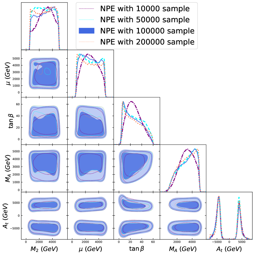
Figure 6: 2D and 1D Posterior distributions of all the parameters coming from NPE method with different sample subsets are shown here. The lighter and darker blue colors represent the $2\sigma$ and $1\sigma$ regions with $10^{5}$ sample subset. The sample subset contours are represented by purple, cyan, blue, and coral colors for $10^{4}$, $5\times 10^{4}$, $10^{5}$, and $2\times 10^{5}$ samples respectively.

Next, we focus on the time taken for training and posterior sample generation. The time consumption for each algorithm is presented in the right panel of Figure 5. It is obvious that the NPE is significantly faster than the other two algorithms. For instance, in the case of $10^{5}$ sample, the NLE (NRE) takes approximately 4 (2) times longer than the NPE. Even for the full sample set, while the posterior sample efficiency is nearly the same across all algorithms, the time consumption for the NLE and NRE remains substantially higher than that for the NPE.

Similar to the TARP test results, these observations on posterior sample efficiency and time consumption further confirm that the NPE algorithm provides superior performance compared to the other two algorithms, even with fewer samples. Based on this analysis, we conclude that the $10^{5}$ sample subset is sufficient to achieve the desired results using the NPE algorithm.

We finally derive the posterior distribution of the allowed parameter space for pMSSM model after satisfying the constraints from Higgs sector and flavor observables. The corresponding corner plots of posterior samples for the NPE algorithm are shown in Figure 6. In this plot, purple, cyan, blue, and coral lines represent subsets with $10^{4}$, $5\times 10^{4}$, $10^{5}$, and $2\times 10^{5}$ samples, respectively. Filled contour plot is shown only for the $10^{5}$ sample subset, while the other subsets are represented with solid or different kinds of dashed lines. It is evident from these plots that there is no significant distinction among the contour plots for subsets with $10^{5}$ samples or more.

At the tree level, the two parameters that describe the MSSM higgs sector are $M_{A}$ and $\tan\beta$. At high $M_{A}$, which is also called the decoupling limitdjouadi2008anatomy ; Djouadi:2013lra , the lighter CP-even state has properties close to that of the SM-like higgs. However, one requires significant loop correction to push the mass to the experimentally measured value. This loop correction is largely obtained from the third generation squarks, especially top squark. Therefore, the top squark mixing parameter $X_{t}=A_{t}-\mu\cot\beta$ plays a big role in determining the higgs mass. This implies a larger $\tan\beta\gtrsim 10$ and large $A_{t}$. This is exactly what we have obtained through our analysis. As evident from Figure 6, the regions with $A_{t}$ close to zero are disfavored and we have obtained two distinct regions for $A_{t}$ beyond 1 TeV on either side of zero. Clearly, the NPE algorithm can efficiently understand this crucial relation between the $A_{t}$ parameter and the SM-like Higgs mass. The value of $\mu$ does not have much impact as long as $A_{t}$ dominates the mixing parameter $X_{t}$. This explains the posterior of $\mu$, which is mostly flat. The parameter $M_{2}$ can only impact the Higgs sector slightly through loop corrections, and hence, the corresponding distribution is also mostly flat.

4.4 $M_{A}-\tan\beta$ contour

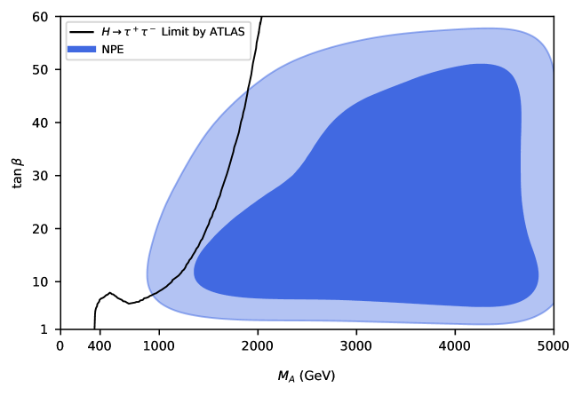
Figure 7: $M_{A}$-$\tan\beta$ contour plot for NPE method with $10^{5}$ sample subset is displayed where darker and lighter blue colors correspond to $1\sigma$ and $2\sigma$ regions respectively. The ATLAS limit coming from $H\to\tau^{+}\tau^{-}$ search is shown by a solid black line.

In this section, we discuss the allowed region for $M_{A}-\tan\beta$ plane determined by the SBI methods. Figure 7 displays the $M_{A}-\tan\beta$ contour plot based on results from the $10^{5}$ sample subset. The lighter and darker blue colors represent the $2\sigma$ and $1\sigma$ contours respectively for NPE algorithm. The allowed region here crucially depends on the flavor observables as well as the higgs sector observables. Constraints arising from the ratio of $\mathcal{B}r(B\to\tau\nu)$ in MSSM and SM depends on the doubly charged higgs mass (determined by $M_{A}$) and $\tan\beta$. Similarly, $\mathcal{B}r(B_{s}\to\mu^{+}\mu^{-})$ varies as $\sim\frac{\tan^{6}\beta}{M_{A}^{4}}$ for large $\tan\beta$. Clearly, a combination of large $\tan\beta$ and small $M_{A}$ should be disfavored from experimental observations. The $\mathcal{B}r(B\to X_{s}\gamma)$ also depends on $M_{A}$ since the charged higgs appears at one loop contribution to the observable. When incorporating Higgs properties alongside these flavor observables, a similar pattern in the $M_{A}-\tan\beta$ plane emerges, consistent with the SBI methods, as shown in Figure 7. The most stringent direct search constraint on the heavy CP-even higgs mass arises from the $H\rightarrow\tau^{+}\tau^{-}$ channel. The ATLAS Collaboration has provided the exclusion limit on Heavy Higgs based on the value of $\tan\beta$ in the Ref. ATLAS:2020zms using Run-II data. We have shown this exclusion limit by the black colored line on this contour plot in Figure. 7. It is clear from the figure that the $1\sigma$ region obtained through the most efficient NPE method is allowed, but part of the $2\sigma$ allowed region is excluded by the experimental result for $M_{A}<$ 2000 GeV. This result is in good agreement with the results provided by Ref. Barman:2024xlc .

5 Summary

In this work, we have addressed a very pertinent issue of parameter space sampling. With large number of input parameters and precisely measured observables it often gets very difficult to identify the most favored parameter space given a particle physics model. Tools like MCMC and nested sampling are efficient but extremely time consuming. The main bottleneck of these algorithms is likelihood computation at each point. In this work, therefore, we have explored the possibility of drawing likelihood-free inference using ML techniques. SBI is one such method that has gained attention in recent times. A subclass of SBI, called amortized, is of particular interest owing to the fact that once properly trained, these methods can generate posterior distributions without getting trained on new data. We have explored three different methods, namely, NPE, NLE, and NRE. In order to ascertain whether these methods can faithfully generate the true posterior distributions of the new physics parameters, we perform the TARP test which can efficiently detect inaccurate inferences. To test this framework, we take a very well-known BSM scenario, namely, the pMSSM. As for observables, we consider the SM-like Higgs mass and signal strengths alongside the flavor observables crucial for constraining the pMSSM parameter space. We observe that the NPE method can faithfully generate the posterior distributions of the input parameters, whereas the NLE and NRE methods fail the TARP test. We have also compared results obtained with training data sets of different sizes and show that with as low as $5\times 10^{4}$ data points, one can generate faithful posterior distributions using the NPE method. It is worth mentioning that we chose to vary only a small set of input parameters for this analysis while keeping all other input parameters fixed at reasonable values that lie beyond the present experimental sensitivity. While this is only done for demonstration purposes and using MCMC will not be too computationally expensive for this particular case study, the advantage of SBI method will be more and more evident with additional experimental data, especially for high dimensional parameter space.

Appendix A Sampling of nine dimensional pMSSM parameter space

In this Appendix A, we consider a nine dimensional pMSSM model by adding four more input parameters - bino, gluino, squarks and slepton masses. We further assume the first 2 generation squarks and all three generation sleptons have equal masses whereas the third genration squark masses are varied independently. The ranges for these nine parameters are listed in Table 5.

Parameter	Range
$M_{1}$	500-5000
$M_{2}$	500-5000
$M_{3}$	500-5000
$\mu$	500-5000
$\tan\beta$	1-60
$M_{A}$	100-5000
$|A_{t}|$	0-8000
$m_{\tilde{q}_{3}}$	1200-5000
$m_{\tilde{q}_{1,2}}=m_{\tilde{l}}$	2000-5000

Table 5: This table represents the range of all the nine free parameters considered for our analysis. All the parameters mentioned here have unit GeV except $\tan\beta$.

As demonstrated in Section 4, the NPE method outperforms the other two SBI methods, we focus exclusively on the results obtained using the NPE method. Approximately 4$\times 10^{6}$ samples were generated, out of which only about $10^{6}$ samples fall within the $3\sigma$ range of the observables. The distributions of these observables for the total sample under consideration are shown in Figure 8.

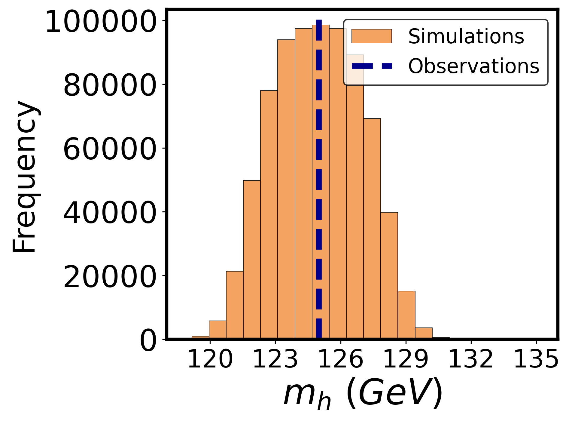
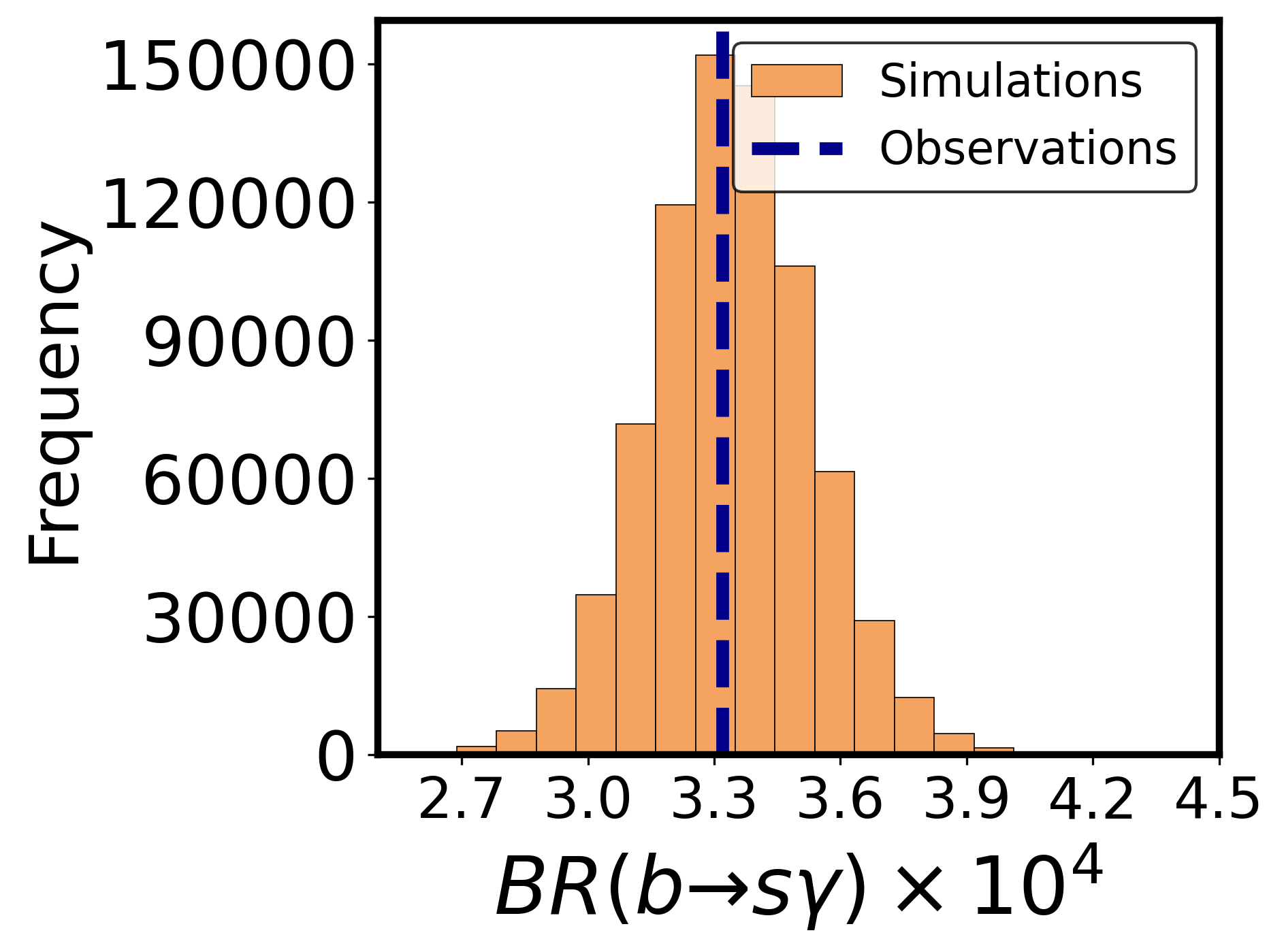
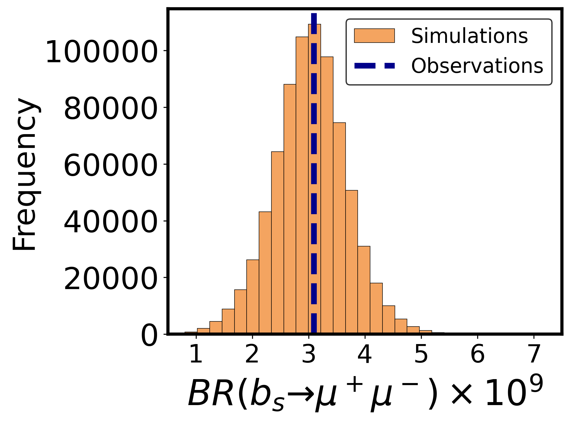
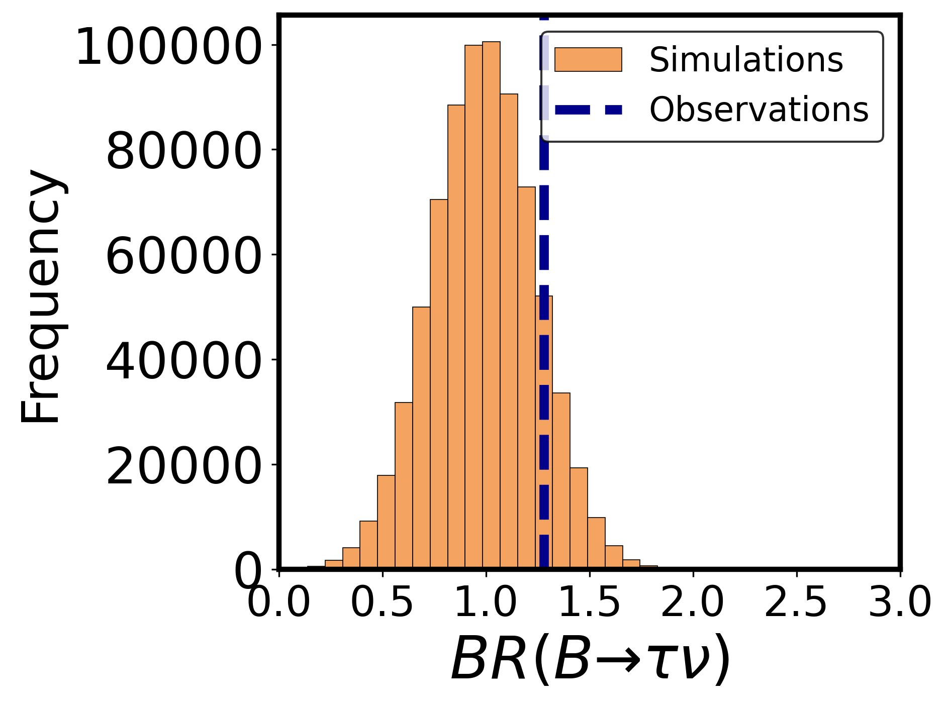
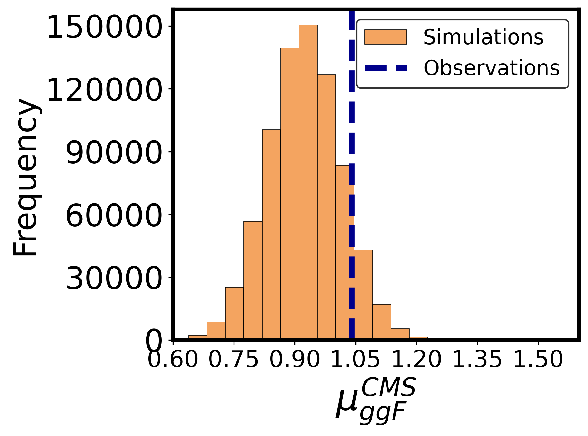
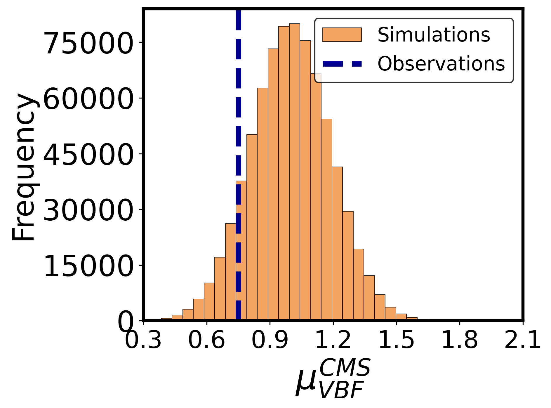
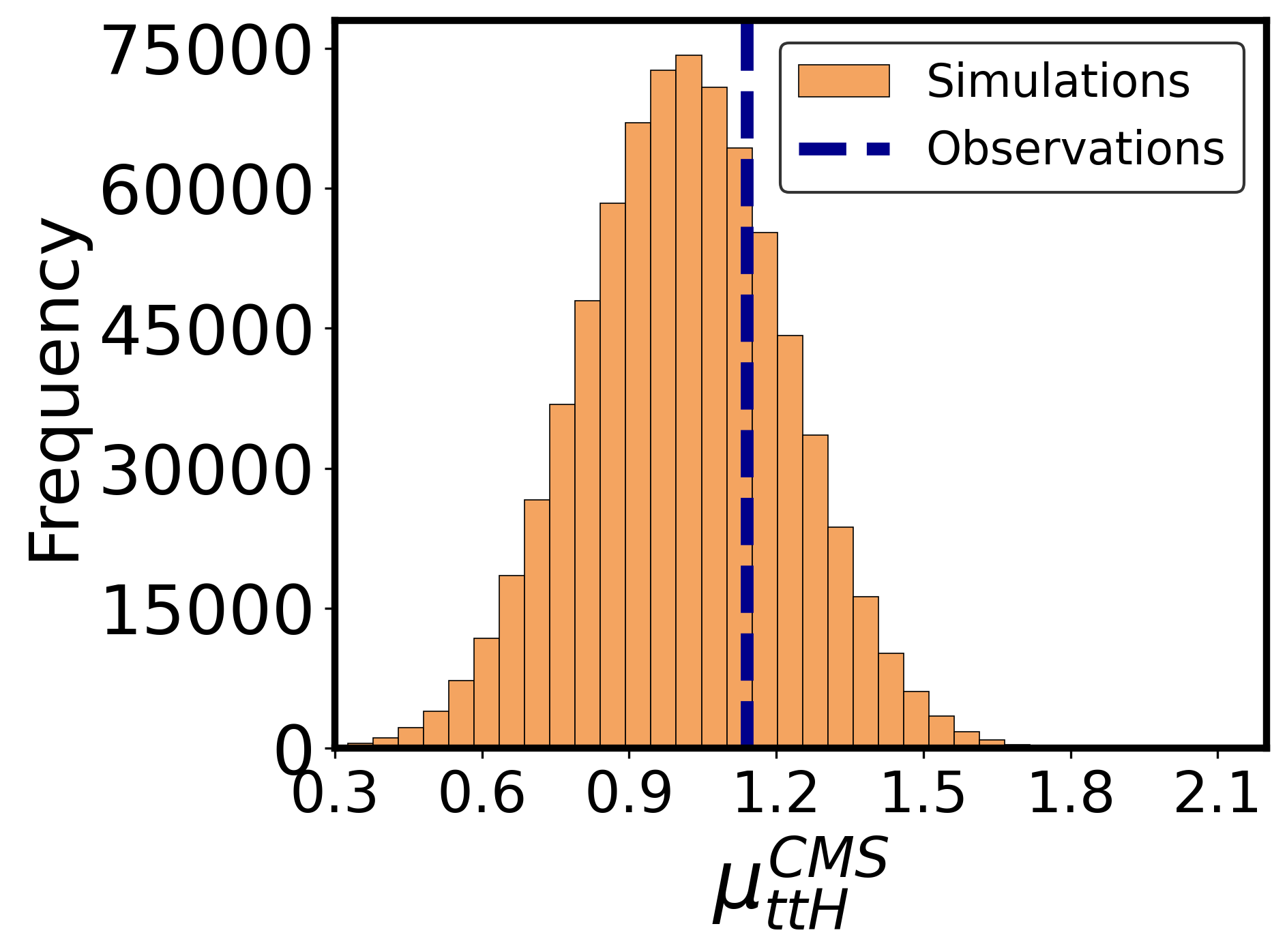
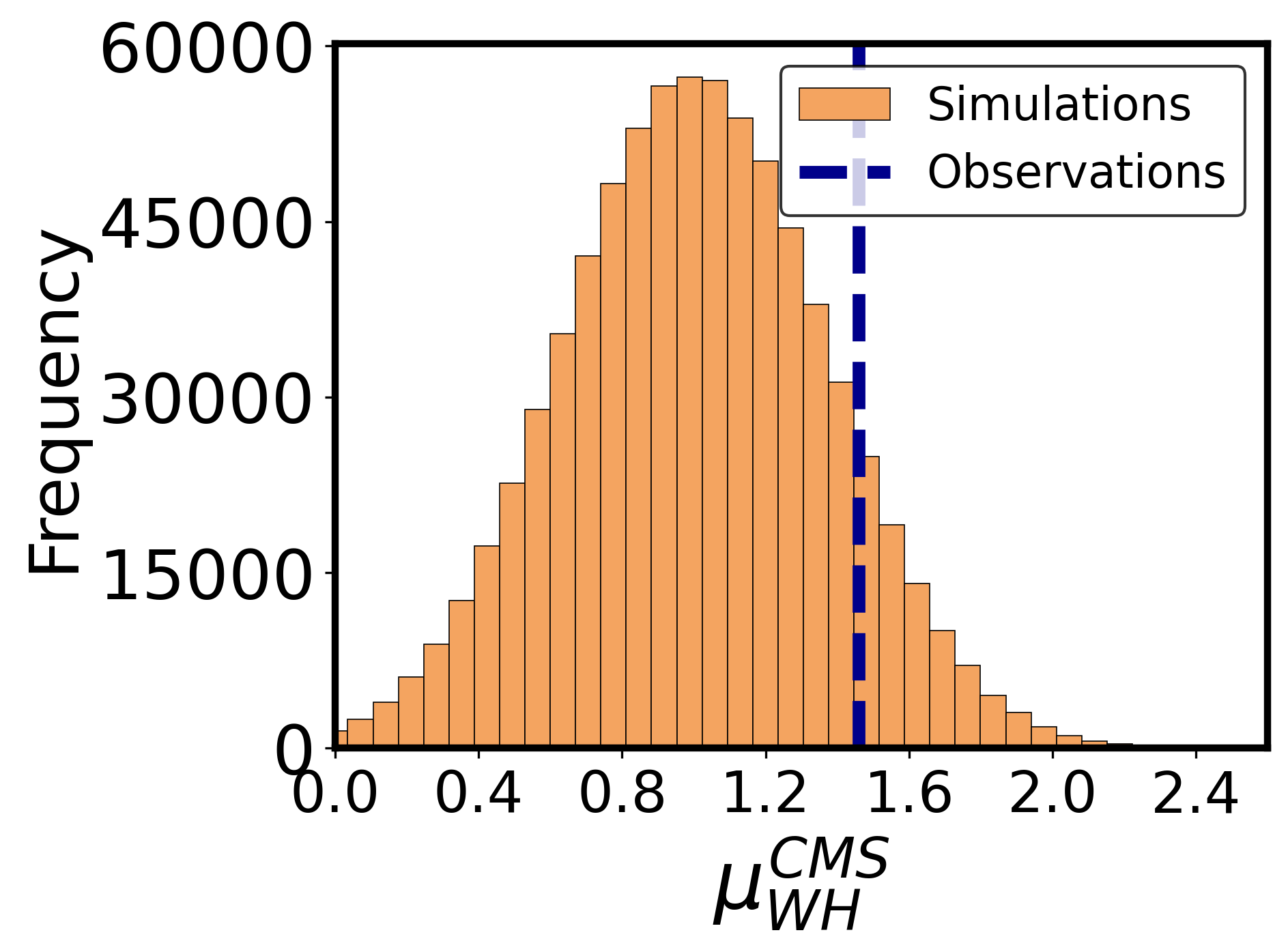
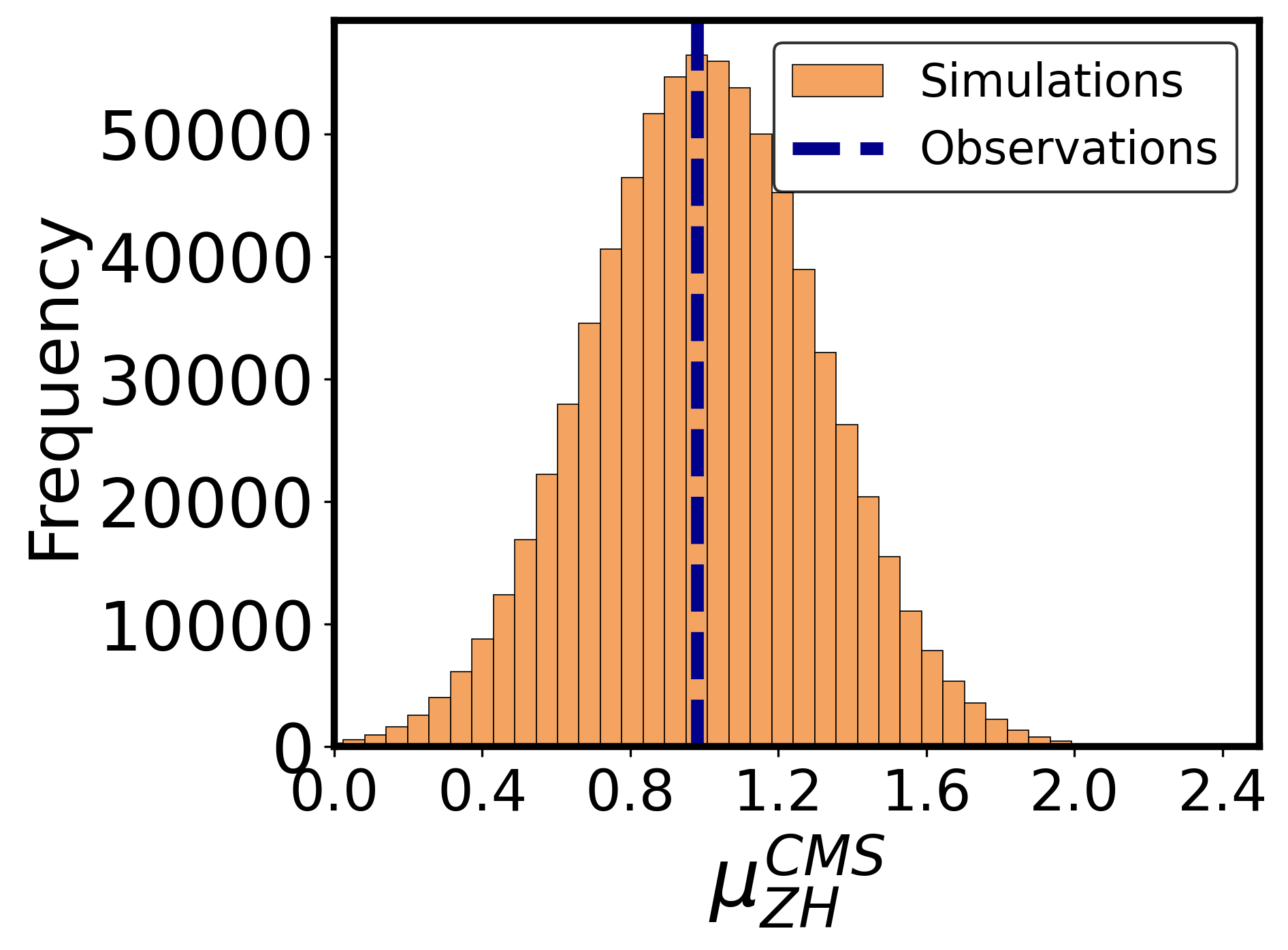
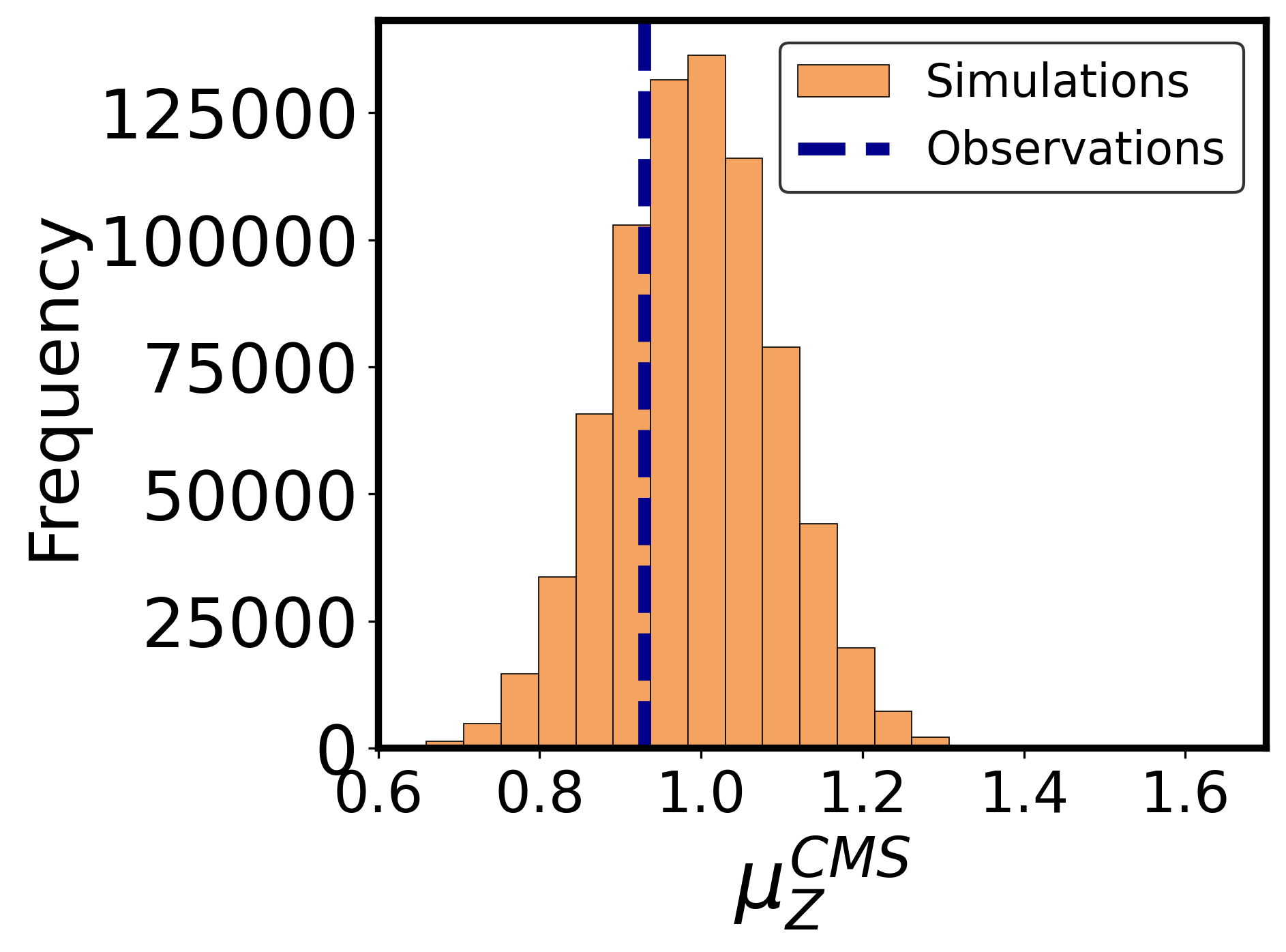
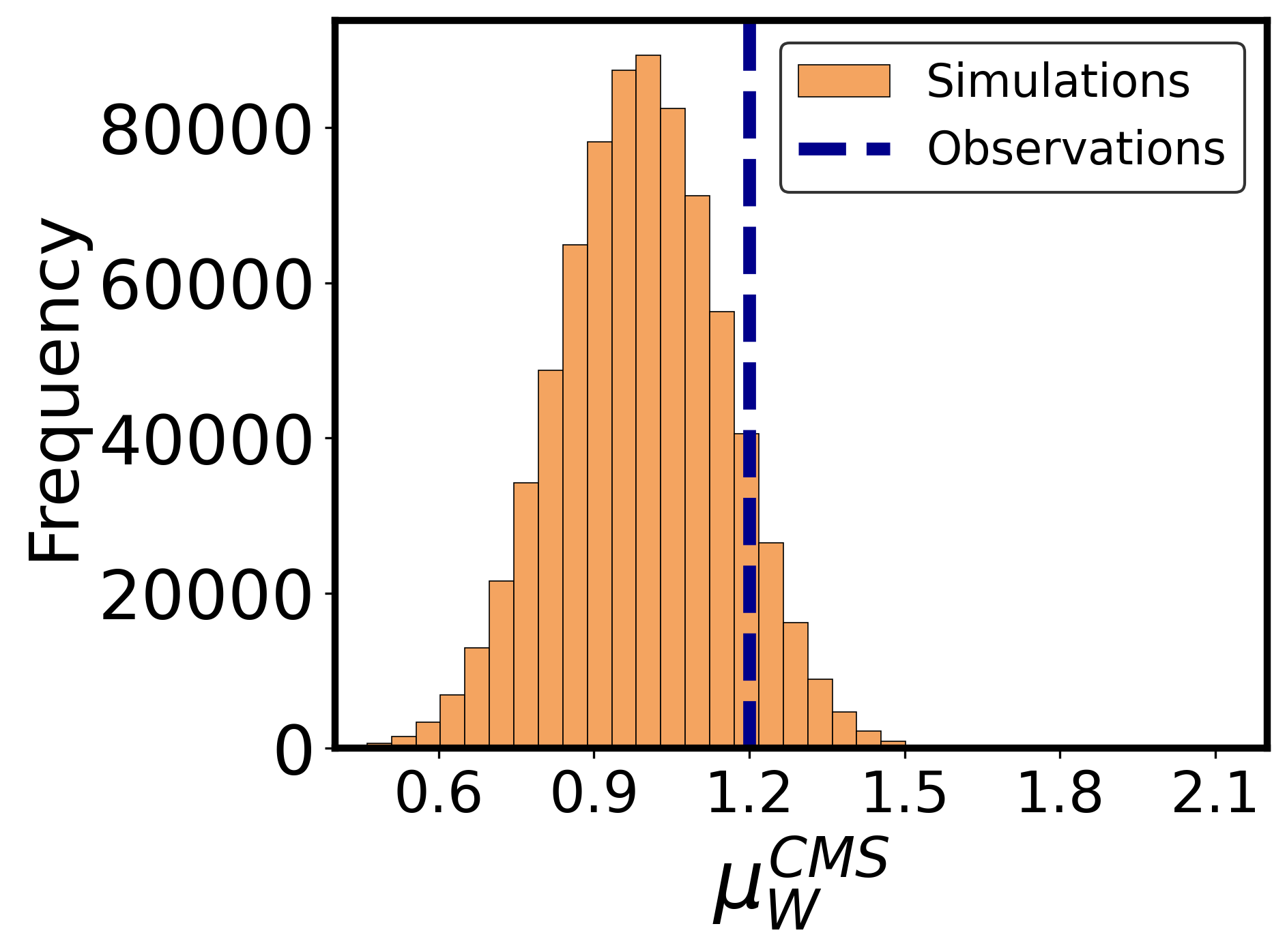
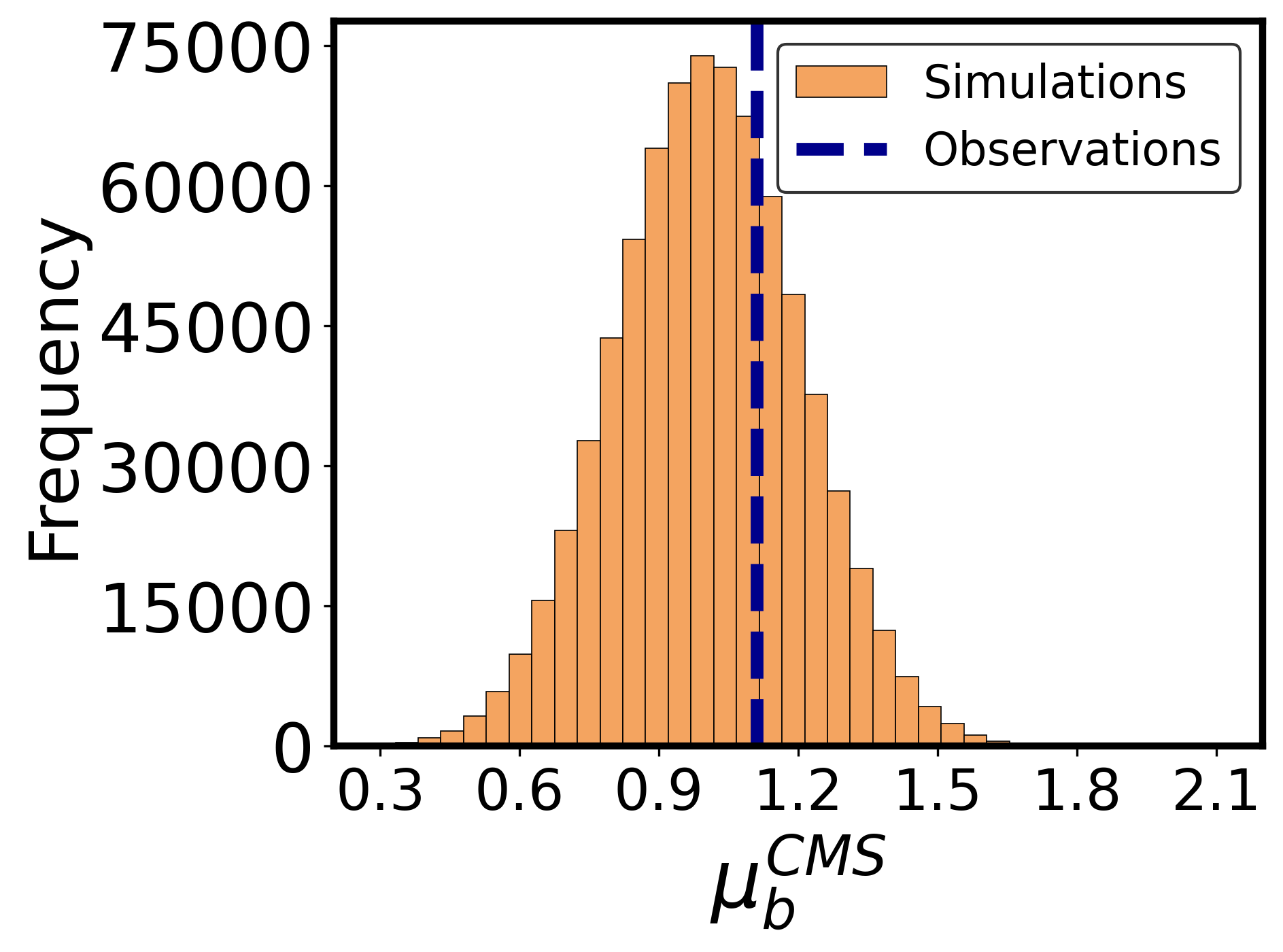
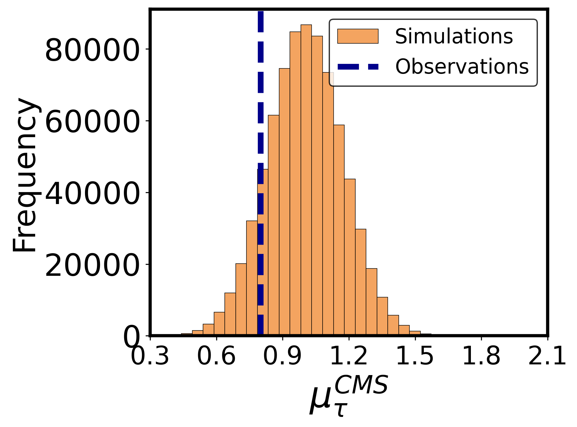
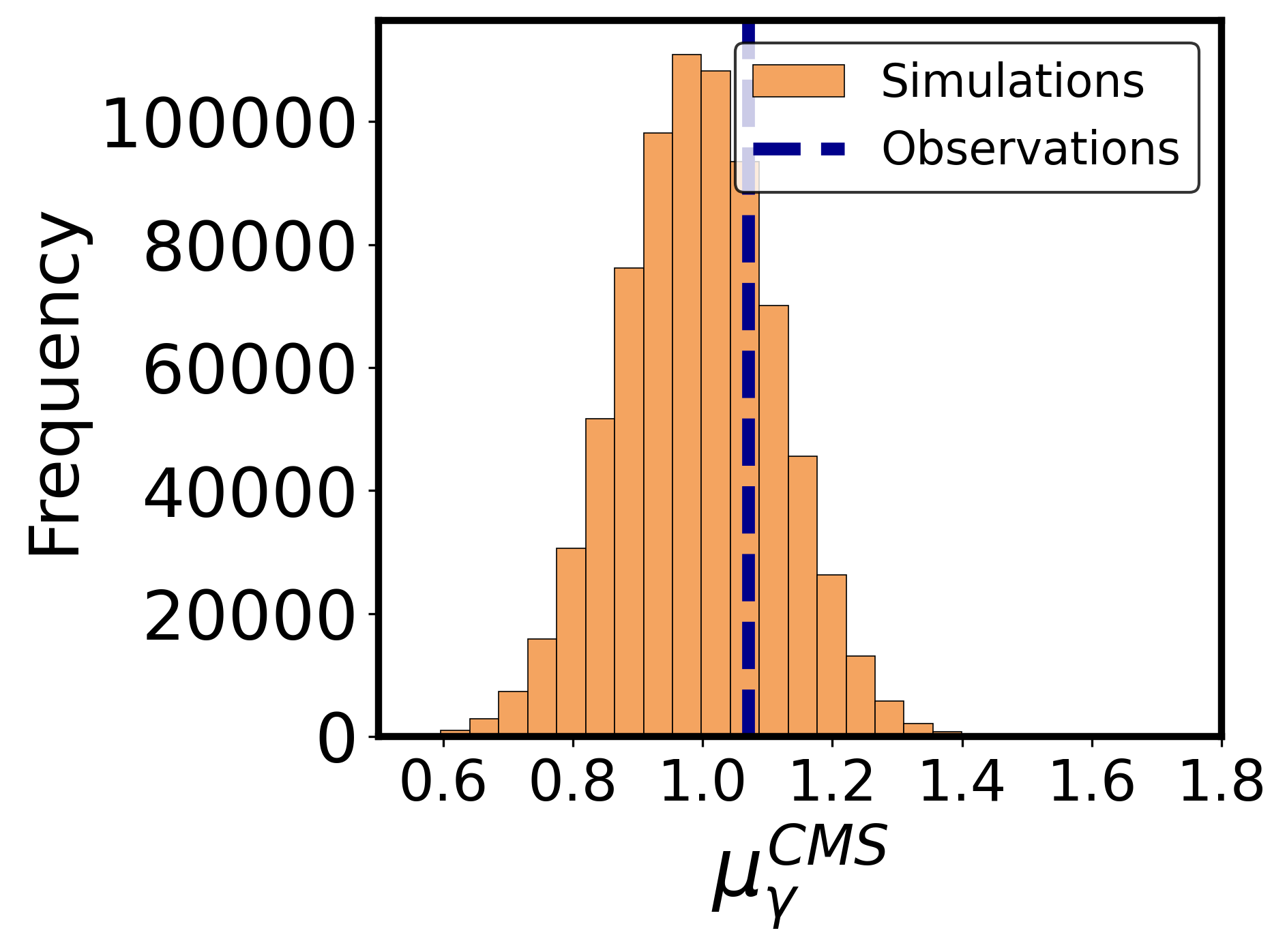
Figure 8: Distributions of all the 14 observables in the training sample after adding the noise are presented by orange-brown color histograms. The dashed blue lines represent the true value of each observable.

Sample subset	$5\times 10^{4}$	$10^{5}$	$2\times 10^{5}$	$4\times 10^{5}$	$6\times 10^{5}$	$8\times 10^{5}$	$10^{6}$
Efficiency (%)	89.8	91.9	94.8	96.9	97.1	97.8	97.4

Table 6: Posterior sample efficiency of different sample subsets.

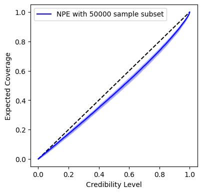
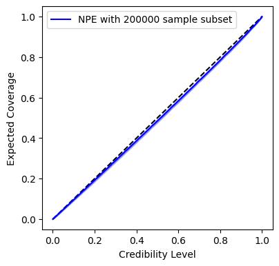
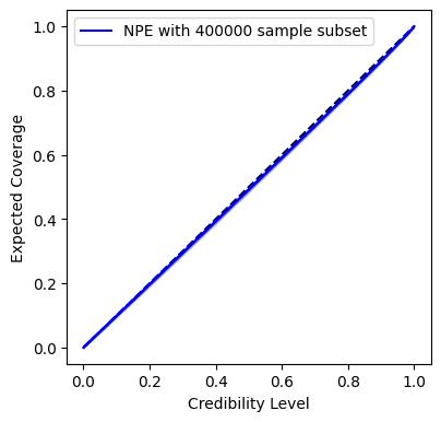
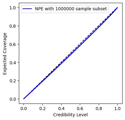
Figure 9: TARP test plots corresponding to $5\times 10^{4}$, $2\times 10^{5}$, $4\times 10^{5}$, $6\times 10^{5}$, $8\times 10^{5}$, $10^{6}$ sample subsets with NPE method for this nine parameter pMSSM are displayed here.

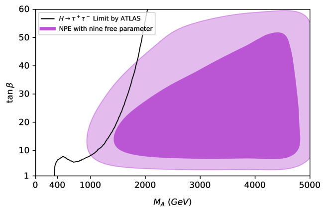
Figure 10: $M_{A}$-$\tan\beta$ contour plot for NPE method with $8\times 10^{5}$ sample subset is displayed where darker and lighter orchid colors correspond to $1\sigma$ and $2\sigma$ regions respectively. The ATLAS limit coming from $H\to\tau^{+}\tau^{-}$ search is shown by a solid black line.

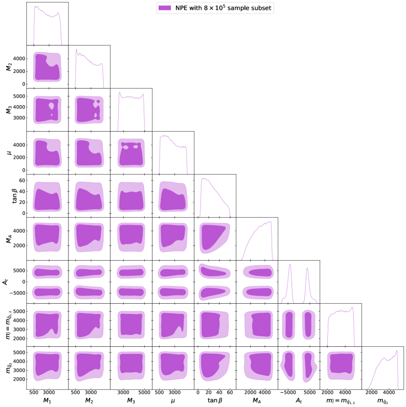
Figure 11: 2D and 1D Posterior distributions of all the nine parameters coming from NPE method with $8\times 10^{5}$ sample subset are shown here. The lighter and darker orchid colors represent the $2\sigma$ and $1\sigma$ regions respectively.

We train the samples in subsets of increasing size, such as $5\times 10^{4}$, $10^{5}$, …, $10^{6}$ and present the posterior sample efficiency in Table 6. It is worth mentioning that as the dimension of the parameter space has increased, we need larger number of samples. From Table 6, it is evident that the posterior sample efficiency increases very slowly beyond the $4\times 10^{5}$ sample subset and maximum efficiency is obtained for $8\times 10^{5}$ sample subset. Therefore, we restrict our analysis to $8\times 10^{5}$ samples. Similarly, from the TARP test plot in Figure 9, we observe that there is no significant difference in the TARP results beyond the $2\times 10^{5}$ sample subset as the sample size increases and subset with $8\times 10^{5}$ sample shows the best result. To be on the conservative side, we consider $8\times 10^{5}$ sample subset result to obtain the allowed $M_{A}-\tan\beta$ contour region. We have shown the contour in Figure. 10, where the filled regions with lighter and darker orchid colors refer to $2\sigma$ and $1\sigma$ regions respectively. Compare to the results of five dimensional case (see Figure 7), we obtain similar parameter regions in Figure 10. It just needs more samples to handle the added complexity. The posterior distributions of all parameters are shown in Figure 11. As discussed in Section 4.3, the parameters $M_{1}$, $M_{2}$, $M_{3}$, and $\mu$ show no direct effect and exhibit mostly flat distributions. Similarly, the slepton masses and second-generation squark masses have a much smaller impact on the Higgs mass, resulting in flat distributions for these parameters as well. The Higgs mass, however, receives significant radiative corrections from the top/stop sector. These corrections are proportional to $\ln\left(\frac{m_{\tilde{t}}^{2}}{m_{t}^{2}}\right)$, with heavier stops providing larger contributions that raise the Higgs mass closer to the observed value ($\sim$ 125 GeV). Interestingly, the posterior also favors higher values of third-generation squark masses, starting from approximately 2000 GeV, even though the scan range was 1200-5000 GeV.

References

- (1) P. F. de Salas, D. V. Forero, S. Gariazzo, P. Martínez-Miravé, O. Mena, C. A. Ternes et al., 2020 global reassessment of the neutrino oscillation picture, JHEP 02 (2021) 071, [2006.11237].
- (2) NOvA collaboration, M. A. Acero et al., First Measurement of Neutrino Oscillation Parameters using Neutrinos and Antineutrinos by NOvA, Phys. Rev. Lett. 123 (2019) 151803, [1906.04907].
- (3) F. Zwicky, Republication of: The redshift of extragalactic nebulae, General Relativity and Gravitation 41 (Jan., 2009) 207–224.
- (4) F. Zwicky, On the Masses of Nebulae and of Clusters of Nebulae, apj 86 (Oct., 1937) 217.
- (5) G. Jungman, M. Kamionkowski and K. Griest, Supersymmetric dark matter, Phys. Rept. 267 (1996) 195–373, [hep-ph/9506380].
- (6) L. Susskind, The gauge hierarchy problem, technicolor, supersymmetry, and all that, Physics Reports 104 (1984) 181–193.
- (7) E. Gildener, Gauge-symmetry hierarchies, Phys. Rev. D 14 (Sep, 1976) 1667–1672.
- (8) BaBar collaboration, J. P. Lees et al., Search for mixing-induced CP violation using partial reconstruction of and kaon tagging, Phys. Rev. D 93 (2016) 032001, [1506.00234].
- (9) LHCb Collaboration collaboration, R. Aaij, A. S. W. Abdelmotteleb, C. Abellan Beteta, F. Abudin, T. Ackernley, B. Adeva et al., Direct violation in charmless three-body decays of mesons, Phys. Rev. D 108 (Jul, 2023) 012008.
- (10) Belle collaboration, L. K. Li et al., Search for CP violation and measurement of branching fractions and decay asymmetry parameters for c+→h+ and c+→0h+ (h=K,), Sci. Bull. 68 (2023) 583–592, [2208.08695].
- (11) BESIII collaboration, H. Miao, Measurements of charmonia decays from BESIII, PoS FPCP2023 (7, 2023) 086, [2307.12565].
- (12) CMS collaboration, S. Chatrchyan et al., Observation of a New Boson at a Mass of 125 GeV with the CMS Experiment at the LHC, Phys. Lett. B 716 (2012) 30–61, [1207.7235].
- (13) ATLAS collaboration, G. Aad et al., Observation of a new particle in the search for the Standard Model Higgs boson with the ATLAS detector at the LHC, Phys. Lett. B 716 (2012) 1–29, [1207.7214].
- (14) G. C. Branco, P. M. Ferreira, L. Lavoura, M. N. Rebelo, M. Sher and J. P. Silva, Theory and phenomenology of two-Higgs-doublet models, Phys. Rept. 516 (2012) 1–102, [1106.0034].
- (15) ATLAS, CMS collaboration, G. Aad et al., Combined Measurement of the Higgs Boson Mass in Collisions at and 8 TeV with the ATLAS and CMS Experiments, Phys. Rev. Lett. 114 (2015) 191803, [1503.07589].
- (16) S. P. Martin, A Supersymmetry primer, Adv. Ser. Direct. High Energy Phys. 18 (1998) 1–98, [hep-ph/9709356].
- (17) MSSM Working Group collaboration, A. Djouadi et al., The Minimal supersymmetric standard model: Group summary report, in GDR (Groupement De Recherche) - Supersymetrie, 12, 1998. hep-ph/9901246.
- (18) R. K. Barman, G. Bélanger, B. Bhattacherjee, R. Godbole and R. Sengupta, Current status of the light neutralino thermal dark matter in the phenomenological MSSM, Phys. Rev. D 111 (2025) 015014, [2402.07991].
- (19) E. Bagnaschi et al., Likelihood Analysis of the pMSSM11 in Light of LHC 13-TeV Data, Eur. Phys. J. C 78 (2018) 256, [1710.11091].
- (20) GAMBIT collaboration, P. Athron et al., A global fit of the MSSM with GAMBIT, Eur. Phys. J. C 77 (2017) 879, [1705.07917].
- (21) R. K. Barman, B. Bhattacherjee, A. Choudhury, D. Chowdhury, J. Lahiri and S. Ray, Current status of MSSM Higgs sector with LHC 13 TeV data, Eur. Phys. J. Plus 134 (2019) 150, [1608.02573].
- (22) B. Bhattacherjee, A. Chakraborty and A. Choudhury, Status of the MSSM Higgs sector using global analysis and direct search bounds, and future prospects at the High Luminosity LHC, Phys. Rev. D 92 (2015) 093007, [1504.04308].
- (23) L. Roszkowski, E. M. Sessolo and A. J. Williams, Prospects for dark matter searches in the pMSSM, JHEP 02 (2015) 014, [1411.5214].
- (24) A. Hammad and R. Ramos, DLScanner: A parameter space scanner package assisted by deep learning methods, 2412.19675.
- (25) M. Binjonaid, Multi-label Classification of Parameter Constraints in BSM Extensions using Deep Learning, 2409.05453.
- (26) M. A. Diaz, S. Dasmahapatra and S. Moretti, hep-aid: A Python Library for Sample Efficient Parameter Scans in Beyond the Standard Model Phenomenology, 2412.17675.
- (27) S. Caron, T. Heskes, S. Otten and B. Stienen, Constraining the Parameters of High-Dimensional Models with Active Learning, Eur. Phys. J. C 79 (2019) 944, [1905.08628].
- (28) M. D. Goodsell and A. Joury, Active learning BSM parameter spaces, Eur. Phys. J. C 83 (2023) 268, [2204.13950].
- (29) J. Hollingsworth, M. Ratz, P. Tanedo and D. Whiteson, Efficient sampling of constrained high-dimensional theoretical spaces with machine learning, Eur. Phys. J. C 81 (2021) 1138, [2103.06957].
- (30) A. Hammad, M. Park, R. Ramos and P. Saha, Exploration of parameter spaces assisted by machine learning, Comput. Phys. Commun. 293 (2023) 108902, [2207.09959].
- (31) N. T. Hunt-Smith, W. Melnitchouk, F. Ringer, N. Sato, A. W. Thomas and M. J. White, Accelerating Markov Chain Monte Carlo sampling with diffusion models, Comput. Phys. Commun. 296 (2024) 109059, [2309.01454].
- (32) M. S. Albergo, D. Boyda, D. C. Hackett, G. Kanwar, K. Cranmer, S. Racanière et al., Introduction to Normalizing Flows for Lattice Field Theory, 2101.08176.
- (33) R. Baruah, S. Mondal, S. K. Patra and S. Roy, Normalizing Flow-Assisted Nested Sampling on Type-II Seesaw Model, 2501.16432.
- (34) J. Brehmer, F. Kling, I. Espejo and K. Cranmer, MadMiner: Machine learning-based inference for particle physics, Comput. Softw. Big Sci. 4 (2020) 3, [1907.10621].
- (35) Y. Zhu and N. Zabaras, Bayesian deep convolutional encoder-decoder networks for surrogate modeling and uncertainty quantification, Journal of Computational Physics 366 (Aug., 2018) 415–447, [1801.06879].
- (36) J. Hermans, V. Begy and G. Louppe, Likelihood-free MCMC with Amortized Approximate Ratio Estimators, arXiv e-prints (Mar., 2019) arXiv:1903.04057, [1903.04057].
- (37) G. Papamakarios and I. Murray, Fast -free inference of simulation models with bayesian conditional density estimation, 1605.06376.
- (38) G. Papamakarios, Neural density estimation and likelihood-free inference, 1910.13233.
- (39) J. Brehmer and K. Cranmer, Simulation-based inference methods for particle physics, 2010.06439.
- (40) H. Bahl, V. Bresó, G. De Crescenzo and T. Plehn, Advancing Tools for Simulation-Based Inference, 2410.07315.
- (41) R. Mastandrea, B. Nachman and T. Plehn, Constraining the Higgs potential with neural simulation-based inference for di-Higgs production, Phys. Rev. D 110 (2024) 056004, [2405.15847].
- (42) ATLAS collaboration, G. Aad et al., An implementation of neural simulation-based inference for parameter estimation in ATLAS, 2412.01600.
- (43) L. Morrison, S. Profumo, N. Smyth and J. Tamanas, Simulation based inference for efficient theory space sampling: An application to supersymmetric explanations of the anomalous muon g-2, Phys. Rev. D 106 (2022) 115016, [2203.13403].
- (44) P. Lemos, A. Coogan, Y. Hezaveh and L. Perreault-Levasseur, Sampling-Based Accuracy Testing of Posterior Estimators for General Inference, 40th International Conference on Machine Learning 202 (Jan., 2023) 19256–19273, [2302.03026].
- (45) C. Hahn et al., Cosmological constraints from non-Gaussian and nonlinear galaxy clustering using the SimBIG inference framework, Nature Astron. 8 (2024) 1457–1467, [2310.15246].
- (46) K. Zhong, M. Gatti and B. Jain, Improving convolutional neural networks for cosmological fields with random permutation, Phys. Rev. D 110 (2024) 043535, [2403.01368].
- (47) D. S. Greenberg, M. Nonnenmacher and J. H. Macke, Automatic posterior transformation for likelihood-free inference, 1905.07488.
- (48) K. Cranmer, J. Pavez and G. Louppe, Approximating likelihood ratios with calibrated discriminative classifiers, 1506.02169.
- (49) D. P. Kingma and J. Ba, Adam: A method for stochastic optimization, 1412.6980.
- (50) G. Papamakarios, T. Pavlakou and I. Murray, Masked autoregressive flow for density estimation, Advances in neural information processing systems 30 (2017) , [1705.07057].
- (51) C. M. Bishop, “Mixture density networks.” http://www.ncrg.aston.ac.uk/, 1994.
- (52) C. Durkan, A. Bekasov, I. Murray and G. Papamakarios, Neural spline flows, 1906.04032.
- (53) G. Papamakarios, D. C. Sterratt and I. Murray, Sequential Neural Likelihood: Fast Likelihood-free Inference with Autoregressive Flows, arXiv e-prints (May, 2018) arXiv:1805.07226, [1805.07226].
- (54) M. Germain, K. Gregor, I. Murray and H. Larochelle, Made: Masked autoencoder for distribution estimation, in Proceedings of the 32nd International Conference on Machine Learning (F. Bach and D. Blei, eds.), vol. 37 of Proceedings of Machine Learning Research, (Lille, France), pp. 881–889, PMLR, 07–09 Jul, 2015. 1502.03509. DOI.
- (55) CMS collaboration, T. C. Collaboration et al., Search for supersymmetry in proton-proton collisions at 13 TeV in final states with jets and missing transverse momentum, JHEP 10 (2019) 244, [1908.04722].
- (56) ATLAS collaboration, G. Aad et al., Search for squarks and gluinos in final states with jets and missing transverse momentum using 139 fb-1 of =13 TeV collision data with the ATLAS detector, JHEP 02 (2021) 143, [2010.14293].
- (57) ATLAS collaboration, G. Aad et al., Search for squarks and gluinos in final states with one isolated lepton, jets, and missing transverse momentum at with the ATLAS detector, Eur. Phys. J. C 81 (2021) 600, [2101.01629].
- (58) CMS collaboration, A. M. Sirunyan et al., Search for top squark production in fully-hadronic final states in proton-proton collisions at 13 TeV, Phys. Rev. D 104 (2021) 052001, [2103.01290].
- (59) CMS collaboration, A. M. Sirunyan et al., Searches for physics beyond the standard model with the variable in hadronic final states with and without disappearing tracks in proton-proton collisions at 13 TeV, Eur. Phys. J. C 80 (2020) 3, [1909.03460].
- (60) CMS collaboration, A. M. Sirunyan et al., Search for physics beyond the standard model in events with jets and two same-sign or at least three charged leptons in proton-proton collisions at 13 TeV, Eur. Phys. J. C 80 (2020) 752, [2001.10086].
- (61) CMS collaboration, A. Tumasyan et al., Search for supersymmetry in final states with a single electron or muon using angular correlations and heavy-object identification in proton-proton collisions at = 13 TeV, JHEP 09 (2023) 149, [2211.08476].
- (62) CMS collaboration, A. M. Sirunyan et al., Search for supersymmetry in final states with two oppositely charged same-flavor leptons and missing transverse momentum in proton-proton collisions at 13 TeV, JHEP 04 (2021) 123, [2012.08600].
- (63) ATLAS collaboration, G. Aad et al., Search for pair production of squarks or gluinos decaying via sleptons or weak bosons in final states with two same-sign or three leptons with the ATLAS detector, JHEP 02 (2024) 107, [2307.01094].
- (64) ATLAS collaboration, G. Aad et al., Searches for new phenomena in events with two leptons, jets, and missing transverse momentum in 139 fb-1 of TeV collisions with the ATLAS detector, Eur. Phys. J. C 83 (2023) 515, [2204.13072].
- (65) ATLAS collaboration, G. Aad et al., Search for electroweak production of charginos and sleptons decaying into final states with two leptons and missing transverse momentum in TeV collisions using the ATLAS detector, Eur. Phys. J. C 80 (2020) 123, [1908.08215].
- (66) ATLAS collaboration, G. Aad et al., Search for charginos and neutralinos in final states with two boosted hadronically decaying bosons and missing transverse momentum in collisions at = 13 TeV with the ATLAS detector, Phys. Rev. D 104 (2021) 112010, [2108.07586].
- (67) CMS collaboration, A. Tumasyan et al., Search for electroweak production of charginos and neutralinos in proton-proton collisions at = 13 TeV, JHEP 04 (2022) 147, [2106.14246].
- (68) CMS collaboration, A. Tumasyan et al., Search for electroweak production of charginos and neutralinos at s=13TeV in final states containing hadronic decays of WW, WZ, or WH and missing transverse momentum, Phys. Lett. B 842 (2023) 137460, [2205.09597].
- (69) CMS collaboration, A. Hayrapetyan et al., Combined search for electroweak production of winos, binos, higgsinos, and sleptons in proton-proton collisions at s=13 TeV, Phys. Rev. D 109 (2024) 112001, [2402.01888].
- (70) CMS collaboration, A. Tumasyan et al., Search for supersymmetry in final states with two or three soft leptons and missing transverse momentum in proton-proton collisions at = 13 TeV, JHEP 04 (2022) 091, [2111.06296].
- (71) ATLAS collaboration, G. Aad et al., Search for chargino–neutralino pair production in final states with three leptons and missing transverse momentum in TeV pp collisions with the ATLAS detector, Eur. Phys. J. C 81 (2021) 1118, [2106.01676].
- (72) ATLAS collaboration, G. Aad et al., Search for long-lived charginos based on a disappearing-track signature using 136 fb-1 of pp collisions at = 13 TeV with the ATLAS detector, Eur. Phys. J. C 82 (2022) 606, [2201.02472].
- (73) CMS collaboration, A. M. Sirunyan et al., Search for disappearing tracks in proton-proton collisions at 13 TeV, Phys. Lett. B 806 (2020) 135502, [2004.05153].
- (74) B. C. Allanach, A. Djouadi, J. L. Kneur, W. Porod and P. Slavich, Precise determination of the neutral Higgs boson masses in the MSSM, JHEP 09 (2004) 044, [hep-ph/0406166].
- (75) CMS collaboration, Combined Higgs boson production and decay measurements with up to 137 fb-1 of proton-proton collision data at = 13 TeV, .
- (76) HFLAV collaboration, Y. S. Amhis et al., Averages of b-hadron, c-hadron, and -lepton properties as of 2018, Eur. Phys. J. C 81 (2021) 226, [1909.12524].
- (77) LHCb collaboration, R. Aaij et al., Analysis of Neutral B-Meson Decays into Two Muons, Phys. Rev. Lett. 128 (2022) 041801, [2108.09284].
- (78) Belle collaboration, K. Hara et al., Evidence for with a Semileptonic Tagging Method, Phys. Rev. D 82 (2010) 071101, [1006.4201].
- (79) Belle collaboration, A. Abdesselam et al., Measurement of the branching fraction of decays with the semileptonic tagging method and the full Belle data sample, in 8th International Workshop on the CKM Unitarity Triangle, 9, 2014. 1409.5269.
- (80) Belle collaboration, B. Kronenbitter et al., Measurement of the branching fraction of decays with the semileptonic tagging method, Phys. Rev. D 92 (2015) 051102, [1503.05613].
- (81) S. Heinemeyer, W. Hollik and G. Weiglein, FeynHiggs: A Program for the calculation of the masses of the neutral CP even Higgs bosons in the MSSM, Comput. Phys. Commun. 124 (2000) 76–89, [hep-ph/9812320].
- (82) S. Heinemeyer, W. Hollik and G. Weiglein, The Masses of the neutral CP - even Higgs bosons in the MSSM: Accurate analysis at the two loop level, Eur. Phys. J. C 9 (1999) 343–366, [hep-ph/9812472].
- (83) H. Bahl and W. Hollik, Precise prediction for the light MSSM Higgs boson mass combining effective field theory and fixed-order calculations, Eur. Phys. J. C 76 (2016) 499, [1608.01880].
- (84) H. Bahl, T. Hahn, S. Heinemeyer, W. Hollik, S. Paß ehr, H. Rzehak et al., Precision calculations in the MSSM Higgs-boson sector with FeynHiggs 2.14, Comput. Phys. Commun. 249 (2020) 107099, [1811.09073].
- (85) G. Belanger, F. Boudjema, A. Pukhov and A. Semenov, micrOMEGAs: Version 1.3, Comput. Phys. Commun. 174 (2006) 577–604, [hep-ph/0405253].
- (86) G. Belanger, F. Boudjema, A. Pukhov and A. Semenov, Dark matter direct detection rate in a generic model with micrOMEGAs 2.2, Comput. Phys. Commun. 180 (2009) 747–767, [0803.2360].
- (87) G. Belanger, F. Boudjema, P. Brun, A. Pukhov, S. Rosier-Lees, P. Salati et al., Indirect search for dark matter with micrOMEGAs2.4, Comput. Phys. Commun. 182 (2011) 842–856, [1004.1092].
- (88) G. Belanger, F. Boudjema, A. Pukhov and A. Semenov, micrOMEGAs3: A program for calculating dark matter observables, Comput. Phys. Commun. 185 (2014) 960–985, [1305.0237].
- (89) G. Belanger, A. Mjallal and A. Pukhov, Recasting direct detection limits within micrOMEGAs and implication for non-standard Dark Matter scenarios, Eur. Phys. J. C 81 (2021) 239, [2003.08621].
- (90) “Crafting summary statistics of SBI.” https://sbi-dev.github.io/sbi/0.22/tutorial/10_crafting_summary_statistics/.
- (91) M. Ho, D. J. Bartlett, N. Chartier, C. Cuesta-Lazaro, S. Ding, A. Lapel et al., LtU-ILI: An All-in-One Framework for Implicit Inference in Astrophysics and Cosmology, The Open Journal of Astrophysics 7 (July, 2024) 54.
- (92) A. Djouadi, The Anatomy of electro-weak symmetry breaking. II. The Higgs bosons in the minimal supersymmetric model, Phys. Rept. 459 (2008) 1–241, [hep-ph/0503173].
- (93) A. Djouadi, Implications of the Higgs discovery for the MSSM, Eur. Phys. J. C 74 (2014) 2704, [1311.0720].
- (94) ATLAS collaboration, G. Aad et al., Search for heavy Higgs bosons decaying into two tau leptons with the ATLAS detector using collisions at TeV, Phys. Rev. Lett. 125 (2020) 051801, [2002.12223].