Neural Guided Diffusion Bridges

Abstract

We propose a novel method for simulating conditioned diffusion processes (diffusion bridges) in Euclidean spaces. By training a neural network to approximate bridge dynamics, our approach eliminates the need for computationally intensive Markov Chain Monte Carlo (MCMC) methods or reverse-process modeling. Compared to existing methods, it offers greater robustness across various diffusion specifications and conditioning scenarios. This applies in particular to rare events and multimodal distributions, which pose challenges for score-learning- and MCMC-based approaches. We propose a flexible variational family for approximating the diffusion bridge path measure which is partially specified by a neural network. Once trained, it enables efficient independent sampling at a cost comparable to sampling the unconditioned (forward) process.

1 Introduction

Diffusion processes play a fundamental role in various fields such as mathematics, physics, evolutionary biology, and, recently, generative models. In particular, diffusion processes conditioned to hit a specific point at a fixed future time, which are often referred to as diffusion bridges, are of great interest in situations where observations constrain the dynamics of a stochastic process. For example, in generative modeling, stochastic imputation between two given images, also known as the image translation task, uses diffusion bridges to model dynamics [Zhou et al., 2024, Zheng et al., 2024]. In the area of stochastic shape analysis and computational anatomy, random evolutions of biological shapes of organisms are modeled as non-linear diffusion bridges, and simulating such bridges is critical to solving inference and registration problems [Arnaudon et al., 2022, Baker et al., 2024a, Yang et al., 2024]. Finally, diffusion bridges play a crucial role in Bayesian inference and parameter estimations based on discrete-time observations. [Delyon and Hu, 2006, van der Meulen and Schauer, 2017, 2018, Pieschner and Fuchs, 2020]

Simulation of diffusion bridges in either Euclidean spaces or manifolds is nontrivial since, in general, there is no closed-form expression for transition densities, which is key to constructing the conditioned dynamics via Doob’s $h$-transform [Rogers and Williams, 2000]. This task has gained a great deal of attention in the past decades [Beskos et al., 2006, Delyon and Hu, 2006, Schauer et al., 2017, Whitaker et al., 2016, Bierkens et al., 2021, Mider et al., 2021, Heng et al., 2022, Chau et al., 2024, Baker et al., 2024a]. Among them, one common approach is to use a proposed bridge process (called guided proposal) as an approximation to the true bridge. Then either MCMC or Sequential Monte Carlo (SMC) methods are deployed to sample the true bridge via the tractable likelihood ratio between the true and proposed bridges. Another solution is to use the score-matching technique [Hyvarinen, 2005, Vincent, 2011] to directly approximate the intractable score of the transition density using gradient-based optimization. Here, a neural network is trained with samples from the forward process [Heng et al., 2022] or adjoint process [Baker et al., 2024b], and plugged into numerical solving schemes, for example, Euler-Maruyama. Several recent studies deal with the extension of bridge simulation techniques beyond Euclidean spaces to manifolds [Sommer et al., 2017, Jensen and Sommer, 2023, Grong et al., 2024, Corstanje et al., 2024]. All of these rely on either a type of guided proposal or score matching.

Both guided-proposal-based and score-learning-based bridge simulation methods have certain limitations: the guided proposal requires a careful choice of a certain “auxiliary process”. Mider et al. [2021] provided various strategies, but it is fair to say that guided proposals are mostly useful when combined with MCMC or Sequential Monte Carlo (SMC) methods. In case of a strongly nonlinear diffusion or high-dimensional diffusion, the simulation of bridges using guided proposals combined with MCMC (most notably the preconditioned Crank-Nicolson (pCN) scheme [Cotter et al., 2013]) or SMC may be computationally demanding. On the other hand, score-matching relies on sampling unconditioned processes, and it performs poorly for bridges conditioned on rare events, as the unconditioned process rarely explores those regions, resulting in inaccurate estimation. Additionally, the canonical score-matching loss requires the inversion of the matrix $\sigma\sigma^{T}$ where $\sigma$ is the diffusivity of the diffusion. This rules out hypo-elliptic diffusions and poses significant computational challenges for high-dimensional diffusions, where this matrix can become close to singularity, further exacerbating the difficulty of obtaining stable and accurate minimization of the loss.

To address these issues, we introduce a new bridge simulation method called the neural guided diffusion bridge. It consists of the guided proposal introduced in Schauer et al. [2017] with an additional superimposed drift term that is parametrized by a neural network. The family of laws on path space induced by such proposals provides a rich variational family for approximating the law of the diffusion bridge. Once the variational approximation has been learned, independent samples can be generated at a cost similar to that of sampling the unconditional (forward) process. The contributions of this paper are as follows:

• We propose a simple diffusion bridge simulation method inspired by the guided proposal framework, avoiding the need for reverse-process modelling or intensive MCMC or SMC updates. Once the network has been trained, obtaining independent samples from the variational approximation is trivial and computationally cheap;

• Unlike score-learning-based simulation methods, which rely on unconditional samples for learning, our method is grounded to learn directly from conditional samples. This results in greater training efficiency.

• We validate the method through numerical experiments ranging from one-dimensional linear to high-dimensional nonlinear cases, offering qualitative and quantitative analyses. Advantages and disadvantages compared to the guided proposal [Mider et al., 2021] and two score-learning-based methods, Heng et al. [2022] and Baker et al. [2024b], are included.

2 Related work

Diffusion bridge simulation: This topic has received considerable attention over the past two decades and it is hard to give a short complete overview. Early contributions are Clark [1990], Chib et al. [2004], Delyon and Hu [2006], Beskos et al. [2006], Lin et al. [2010], and Golightly and Wilkinson [2010]. The approach of guided proposals that we use here was introduced in Schauer et al. [2017] for fully observed uniformly elliptic diffusions and later extend to partially observed hypo-elliptic diffusions in Bierkens et al. [2020].

Another class of methods approximate the intractable transition density using machine learning or kernel-based techniques. Heng et al. [2022] applied score-matching to define a variational objective for learning the additional drift in the reversed diffusion bridge. Baker et al. [2024b] proposed learning the additional drift directly in the forward bridge via sampling from an adjoint process. Chau et al. [2024] leveraged Gaussian kernel approximations for drift estimation.

The method we propose is a combination of existing ideas. It used the guided proposals from Schauer et al. [2017] to construct a conditioned process, but learns an additional drift term parametrized by a neural net using variational inference.

Diffusion Schrödinger bridge: The diffusion bridge problem addressed in this paper may appear similar to the diffusion Schrödinger bridge (DSB) problem due to their names, but they are fundamentally different. A diffusion bridge refers to a diffusion process conditioned to start at one fixed point and reach another fixed point, while the DSB involves connecting two fixed marginal distributions and is often framed as an entropy-regularized optimal transport problem. Although DSB has gained attention for applications in generative modelling [Thornton et al., 2022, De Bortoli et al., 2021, Shi et al., 2024, Tang et al., 2024], it is important to recognize the distinctions between these problems.

Neural SDE: Neural SDEs extend neural ODEs [Chen et al., 2018] by incorporating inherent stochasticity, making them suitable for modelling data with stochastic dynamics. Research on neural SDEs can be broadly categorized into two areas: (1) modelling terminal state data [Tzen and Raginsky, 2019a, b], and (2) modelling entire data trajectories [Li et al., 2020, Kidger et al., 2021]. Our method aligns with the second category, as it employs trainable drift terms and incorporates end-point constraints to model the full data trajectory.

3 Preliminaries: recap on guided proposals

3.1 Problem statement

Let $(\Omega,\mathcal{F},\mathbb{P})$ be a probability space with filtration $\{\mathcal{F}_{t}\}_{t\in[0,T]}$ and $W$ be a $d_{w}$-dimensional $\mathbb{P}$-Wiener process. A $d$-dimensional $\{\mathcal{F}_{t}\}$-adapted diffusion process $X$ with the law of $\mathbb{P}$ is defined as the strong solution to the stochastic differential equation (SDE):

$$\mathrm{d}X_{t}=b(t,X_{t})\mathrm{d}t+\sigma(t,X_{t})\mathrm{d}W_{t},\quad X_{0}=x_{0}\in\mathbb{R}^{d}.$$ (1)

The coefficient terms $b,\sigma$ are assumed to be Lipschitz continuous and of linear growth to guarantee the existence of a strong solution $X_{t}$ [Øksendal, 2014, Chapter 5.2]. In addition, we impose the standing assumption that $X$ admits smooth transition densities $p$ with respect to the Lebesgue measure $\lambda$ on $(\mathbb{R}^{d},\mathcal{B}(\mathbb{R}^{d}))$, where $\mathcal{B}(\mathbb{R}^{d})$ is the Borel algebra of $\mathbb{R}^{d}$. That is, $\mathbb{P}(X_{t}\in A\mid X_{s}=x)=\int_{A}p(t,y\mid s,x)\lambda(\mathrm{d}y)$ for $0\leq s<t\leq T$, $A\subset\mathbb{R}^{d}$.

Notation 1.

Let $\mathbb{P}^{\circ},\mathbb{P}^{\star}$ and $\mathbb{P}^{\bullet}$ be measures on $(\Omega,\mathcal{F})$, we denote the laws of $X$ on $\mathcal{C}([0,T],\mathbb{R}^{d})$ under $\mathbb{P}^{\circ},\mathbb{P}^{\star}$ and $\mathbb{P}^{\bullet}$ by $\mathbb{L}^{\circ},\mathbb{L}^{\star}$ and $\mathbb{L}^{\bullet}$ respectively. For notational ease, the expectations under $\mathbb{P}^{\circ},\mathbb{P}^{\star}$ and $\mathbb{P}^{\bullet}$ (and similarly $\mathbb{L}^{\circ},\mathbb{L}^{\star}$ and $\mathbb{L}^{\bullet}$) are denoted by $\mathbb{E}^{\circ},\mathbb{E}^{\star}$ and $\mathbb{E}^{\bullet}$ respectively. The process $X$ under $\mathbb{L}^{\circ}$ and $\mathbb{L}^{\bullet}$ is sometimes denoted by $X^{\circ}$ and $X^{\bullet}$ respectively. For any measure $\mathbb{Q}$ on $(\Omega,\mathcal{F})$, we always denote its restriction to $\mathcal{F}_{t}$ by $\mathbb{Q}_{t}$.

The following proposition combines Proposition 4.4 and Example 4.6 in Pieper-Sethmacher et al. [2024]. It shows how the dynamics of $X$ change under observing certain events at time $T$.

Proposition 1.

Fix $t<T$. Let $y\in\mathbb{R}^{d}$ and $q(\cdot\mid y)$ be a probability density function with respect to a finite measure $\nu$. Let $h(t,x)=\int_{\mathbb{R}^{d}}p(T,y\mid t,x)q(v\mid y)\nu(\mathrm{d}y)$, and define the measure $\mathbb{P}^{\star}_{t}$ on $\mathcal{F}_{t}$ by $\mathrm{d}\mathbb{P}^{\star}_{t}\coloneq\frac{h(t,X_{t})}{h(0,x_{0})}\mathrm{d}\mathbb{P}_{t}$. Then under the new measure $\mathbb{P}^{\star}_{t}$, the process $X$ solves the SDE

$$\mathrm{d}X_{t}=\{b(t,X_{t})+a(t,X_{t})r(t,X_{t})\}\mathrm{d}t+\sigma(s,X_{s})\mathrm{d}W^{\star}_{s},\quad X_{0}=x_{0}.$$ (2)

where $r(s,x)=\nabla_{x}\log h(s,x)$, $a(s,x)=\sigma(s,x)\sigma^{T}(s,x)$ and $W^{\star}$ is a $\mathbb{P}^{\star}$-Wiener process.

Furthermore, for any bounded and measurable function $g$ and $0\leq t_{1}\leq...\leq t_{n}<T$,

$$\mathbb{E}^{\star}[g(X_{t_{1}},...,X_{t_{n}})]=\int_{\mathbb{R}^{d}}\mathbb{E}[g(X_{t_{1}},...,X_{t_{n}})\mid X_{T}=y]\,\xi(\mathrm{d}y),$$ (3)

where $\xi$ is the measure defined on $(\mathbb{R}^{d},\mathcal{B}(\mathbb{R}^{d}))$ via

$$\xi(\mathrm{d}y)=\frac{p(T,y\mid 0,x_{0})q(v\mid y)\nu(\mathrm{d}y)}{\int_{\mathbb{R}^{d}}p(T,y\mid 0,x_{0})q(v\mid y)\nu(\mathrm{d}y)}.$$ (4)

A Bayesian interpretation of this result is obtained by assigning the endpoint $y$ a prior density $\pi(y)=p(T,y\mid 0,x_{0})$, and where the observation is given by $v\in\mathbb{R}^{d^{\prime}}$. The likelihood of this observation is $\ell(y\mid v)=q(v\mid y)$ and therefore $\xi(\mathrm{d}y)$ gives the posterior measure of $y$, conditioned on observing $v$. Therefore, under $\mathbb{P}^{\star}$, the process $X$ is constructed by first sampling the endpoint $y$ conditioned on the observation $v$ by $\ell(y\mid v)$, followed by sampling the bridge to $y$. In this paper, we will apply this result when $q(v\mid y)=\psi(v;Ly,\Sigma)$, where $L\in\mathbb{R}^{d\times d^{\prime}}$ with $d^{\prime}\leq d$ and $L$ is assumed to be of full (row) rank. Here, $\psi(x;\mu,\Sigma)$ denotes the density of the $\mathcal{N}(\mu,\Sigma)$-distribution, evaluated at $x$. For example, for a two-dimensional diffusion observing only the first component with small error corresponds to $L=\begin{bmatrix}1&0\end{bmatrix}$ and $\Sigma=\epsilon^{2}\mathbf{I}$, taking $\epsilon$ very small.

If $p$ were known in closed form, then the conditioned process could be directly sampled from Equation (2). This is rarely the case. For this reason, let $\tilde{X}$ be an auxiliary diffusion process that admits transition densities $\tilde{p}$ in closed form. Let $\tilde{h}(t,x)=\int_{\mathbb{R}^{d}}\tilde{p}(T,y\mid t,x)q(v\mid y)\nu(\mathrm{d}y)$. Define

$$E_{t}\coloneq\frac{\tilde{h}(t,X_{t})}{\tilde{h}(0,x_{0})}\exp\left(\int_{0}^{t}\frac{(\partial_{s}+\mathcal{A})\tilde{h}}{\tilde{h}}(s,X_{s})\mathrm{d}s\right),$$ (5)

where $\mathcal{A}$ is the infinitesimal generator of the process $\tilde{X}$, i.e. for any $f$ in its domain $\mathcal{A}f(x)=\sum_{i}b_{i}(t,x)\partial_{i}f(t,x)+\frac{1}{2}\sum_{i,j}a_{i,j}(t,x)\partial_{ij}f(t,x)$. Under weak conditions (see e.g. Palmowski and Rolski [2002, Lemma 3.1]), $E_{t}$ is a mean-one martingale. If we define the change of measure $\mathrm{d}\mathbb{P}^{\circ}_{t}=E_{t}\mathrm{d}\mathbb{P}_{t}$, then, under $\mathbb{P}^{\circ}_{t}$, the process $X$ solves the SDE

$$\mathrm{d}X_{t}=\{b(t,X_{t})+a(t,X_{t})\tilde{r}(t,X_{t})\}\mathrm{d}t+\sigma(t,X_{t})\mathrm{d}W^{\circ}_{t},\quad X_{0}=x_{0},$$ (6)

where $\tilde{r}(t,x)=\nabla_{x}\log\tilde{h}(t,x)$ and $W^{\circ}$ is a $\mathbb{P}^{\circ}$-Wiener process. The process specified by the dynamics in Equation (6) is called the guided proposal, which is a process constructed to resemble the true conditioned process by replacing $r$ by $\tilde{r}$. Crucially, as its drift and diffusion coefficients are known in closed form, the guided proposal can be sampled using efficient numerical SDE solvers.

In Schauer et al. [2017] and Bierkens et al. [2020], precise conditions are given under which $\mathbb{P}^{\star}_{T}\ll\mathbb{P}^{\circ}_{T}$. In the case of conditioning on the event $\{LX_{T}=v\}$ –so there is no noise on the observation– this is subtle. We postpone a short discussion on this to Section 3.3. In all numerical examples considered in Section 5, we have ensured sufficient conditions are satisfied. This guarantees good behaviour when the noise level of the observation noise tends to zero. We then get the following theorem from Bierkens et al. [2020, Theorem 2.6] that states the change of laws from $\mathbb{L}^{\circ}$ to $\mathbb{L}^{\star}$.

Theorem 1.

If certain assumptions [Bierkens et al., 2020, Assumptions 2.4, 2.5] hold, then

$$\frac{\mathrm{d}\mathbb{L}^{\star}}{\mathrm{d}\mathbb{L}^{\circ}}(X)=\frac{\tilde{h}(0,x_{0})}{h(0,x_{0})}\Psi_{T}(X),$$ (7)

where

$$\Psi_{T}(X)=\exp\left(\int_{0}^{T}\frac{(\partial_{t}+\mathcal{A})\tilde{h}}{\tilde{h}}(s,X_{s})\mathrm{d}s\right).$$ (8)

3.2 Guided proposal induced by linear process

We now specialize to the case where the auxiliary process is linear, i.e.

$$\mathrm{d}\tilde{X}_{t}=\tilde{b}(t,\tilde{X}_{t})\mathrm{d}t+\tilde{\sigma}(t)\mathrm{d}W_{t},$$ (9a)

$$\tilde{b}(t,x):=\beta(t)+B(t)x.$$ (9b)

Let $\tilde{A}$ denote the infinitesimal generator of the process $\tilde{X}$. Since $\tilde{h}$ solves $(\partial_{t}+\tilde{A}\tilde{)}h=0$, we can replace $(\partial_{t}+\mathcal{A})\tilde{h}$ by $(\mathcal{A}-\tilde{\mathcal{A}})\tilde{h}$. This gives

$$\Psi_{t}(X)=\exp\left(\int^{t}_{0}G(s,X_{s})\mathrm{d}s\right),\quad t\leq T$$ (10a)

$$G(s,x):=\left\langle b(s,x)-\tilde{b}(s,x),\tilde{r}(s,x)\right\rangle$$

$$-\frac{1}{2}\mathrm{Tr}\left([a(s,x)-\tilde{a}(s)]\left[\tilde{H}(s)-(\tilde{r}\tilde{r}^{T})(s,x)\right]\right).$$ (10b)

Here, $\tilde{H}(s)$ is the negative Hessian of $\log\tilde{h}(s,x)$, which turns out to be independent of $x$, $\tilde{a}(s)=(\tilde{\sigma}\tilde{\sigma}^{T})(s)$. Under the choice of $q(v\mid y)=\psi(v;Ly,\Sigma)$ and $\tilde{X}$, $\tilde{H}$ and $\tilde{r}$ are given by

$$\tilde{H}(t) =L^{T}(t)M(t)L(t)$$ (11a)

$$\tilde{r}(t,x) =L^{T}(t)M(t)(v-u(t)-L(t)x),$$ (11b)

where $M(t)=(M^{{\dagger}}(t))^{-1}$ and $L$, $M^{\dagger}$ and $u$ satisfy the backward ordinary differential equations (ODEs) (See Mider et al. [2021, Theorem 2.4]):

$$\mathrm{d}L(t) =-L(t)B(t)\mathrm{d}t,\quad L(T)=L$$ (12a)

$$\mathrm{d}M^{{\dagger}}(t) =-L(t)\tilde{a}(t)L^{T}(t)\mathrm{d}t,\quad M^{{\dagger}}(T)=\Sigma$$ (12b)

$$\mathrm{d}u(t) =-L(t)\beta(t)\mathrm{d}t,\quad u(T)=0.$$ (12c)

3.3 Choice of linear process

The linear process is defined by the triplet of functions $(\beta,B,\tilde{\sigma})$. In choosing this triplet, two considerations are of importance:

1. In case of conditioning on the event $\{LX_{T}=v\}$ –so no extrinsic noise on the observation– the triplet needs to satisfy certain “matching conditions” to ensure $\mathbb{P}^{\star}\ll\mathbb{P}^{\circ}$. For uniformly elliptic diffusions, this only affects $\tilde{\sigma}$. In case $L=\mathbf{I}_{d}$, so the conditioning is on the full state, $\tilde{\sigma}$ should be chosen such that $\tilde{a}(T)=a(T,x_{T})$. Hence, for this setting, we can always ensure absolute continuity. For the partially observed case, it is necessary to assume that $a$ is of the form $a(t,x)=s(t,Lx)$ for some matrix values map $s$. In that case, it suffices to choose $\tilde{a}$ such that $L\tilde{a}(T)L^{T}=Ls(T,v)L^{T}$. In case the diffusivity does not depend on the state, a natural choice is to take $\tilde{\sigma}=\sigma$ to guarantee absolute continuity.

   For hypo-elliptic diffusions, the restrictions are a bit more delicate. On top of conditions on $\tilde{\sigma}$, it is also required to match certain properties in the drift by choice of $B$. In the examples that we consider in Section 5 we have ensured these properties are satisfied. We refer to Bierkens et al. [2020] for precise conditions and a host of examples.

2. Clearly, the closer $\tilde{b}$ to $b$ and $\tilde{a}$ to $a$, the more the guided proposal resembles the true conditioned process. This can for instance be seen from $\log\Psi_{T}(X)=\int_{0}^{T}\frac{(\mathcal{A}-\tilde{\mathcal{A}})\tilde{h}}{\tilde{h}}(s,X_{s})\mathrm{d}s$, which vanishes if the coefficients are equal. As proposed in Mider et al. [2021], a practical approach is to compute the first-order Taylor expansion at the point one conditions on, i.e., $\beta(t)=b(t,v),B(t)x=J_{b}(t,v)(x-v)$, where $J_{b}$ is the Jacobian of $b(t,x)$ with respect to $x$. Compared to simply taking a scaled Brownian motion, this choice can result in a guided proposal that better mimics true conditioned paths.

3.4 Strategies for improving upon guided proposals

Although the guided proposal takes the conditioning into account, its sample paths may severely deviate from true conditioned paths. This may specifically be the case for strong nonlinearity in the drift or diffusivity. There are different ways of dealing with this.

• If we write the guided path as functional of the driving Wiener process, one can update the driving Wiener increments using the pCN within a Metropolis-Hastings algorithm. Details are provided in Appendix A.1, see also the discussion in Mider et al. [2021].

• Devising better choices for $(\beta,B,\tilde{\sigma})$.

• Adding an extra term to the drift of the guided proposal by a change of measure, where a neural network parametrizes this term. We take this approach here and further elaborate on it in the upcoming section.

4 Methodology

4.1 Neural guided bridge

For a specific diffusion model, it may be hard to specify the maps $B$, $\beta$ and $\tilde{\sigma}$, which may lead to a guided proposal whose realizations look rather different from the actual conditioned paths. For this reason, we propose to adjust the dynamics of the guided proposal by adding a learnable bounded term $\sigma(t,x)\vartheta_{\theta}(t,x)$ to the drift. Specifically, let $\vartheta_{\theta}\colon[0,T]\times\mathbb{R}^{d}\to\mathbb{R}^{d}$ be a function parameterized by $\theta\in\Theta$, where $\Theta$ denotes the parameter space. Assume $x\mapsto\vartheta_{\theta}(t,x)$ is Lipschitz continuous, uniformly over $t\in[0,T]$ and that $\mathbb{P}\left(\int_{0}^{T}\|\vartheta_{\theta}(t,X_{t})\|^{2}\mathrm{d}t<\infty\right)=1$. Let

$$\kappa_{T}\coloneq\exp\left(\int_{0}^{T}\vartheta^{T}_{\theta}(t,X_{t})\mathrm{d}W_{t}^{\circ}-\frac{1}{2}\int_{0}^{T}\|\vartheta_{\theta}(t,X_{t})\|^{2}\mathrm{d}t\right),$$ (13)

and assume $\mathbb{E}[\kappa_{T}]=1$. We refer to Liptser and Shiryaev [2001, Chapter 6] for easily verifiable conditions on $\vartheta_{\theta}$ to ensure this assumption is met. Boundedness of $\vartheta_{\theta}$ for example suffices. Define a new probability measure $\mathbb{P}^{\bullet}$ on $(\Omega,\mathcal{F}_{T})$ by

$$\mathrm{d}\mathbb{P}^{\bullet}\coloneq\kappa_{T}\mathrm{d}\mathbb{P}^{\circ}$$ (14)

By Girsanov’s theorem, the process $W_{t}^{\bullet}\coloneq W^{\circ}_{t}-\int_{0}^{t}\vartheta_{\theta}(s,X_{s})\mathrm{d}s$ is a $\mathbb{P}^{\bullet}$-Wiener process. Therefore, under $\mathbb{P}^{\bullet}$, the process $X$ satisfies the SDE

$$\mathrm{d}X_{t}=b^{\bullet}_{\theta}(t,X_{t})\mathrm{d}t+\sigma(t,X_{t})\mathrm{d}W^{\bullet}_{t},$$

$$b^{\bullet}_{\theta}(s,x)=b^{\circ}(s,x)+\sigma(s,x)\vartheta_{\theta}(s,x),\quad X_{0}=x_{0}.$$ (15)

We also need Assumption 1 to ensure Equation (15) has a strong solution $X_{t}^{\bullet}$.

Assumption 1.

There exist some constants $C,C^{\prime}>0$, such that for any $x,y\in\mathbb{R}^{d}$,

$$\|\vartheta_{\theta}(t,x)-\vartheta_{\theta}(t,y)\|\leq C\|x-y\|,$$ (16)

$$\|\vartheta_{\theta}(t,x)\|^{2}\leq C^{\prime}(1+\|x\|^{2})$$ (17)

We propose to construct $\vartheta_{\theta}$ as a learnable neural network, whose goal is to approximate the difference of drift coefficients. When $\vartheta_{\theta_{\text{opt}}}=\sigma^{T}(r-\tilde{r})$, the discrepancy between $\mathbb{P}^{\bullet}$ and $\mathbb{P}^{\star}$ vanish. In practice, when parameterization is realized as a finite neural network, the Lipschitz continuity can be achieved by plugging in enough smooth activation functions like sigmoid or tanh, and weight normalization or gradient clipping can prevent extreme growth on $x$. In the experiment part, we deploy tanh as activations and gradient clipping by the norm of 1.0 throughout all the experiments to fulfil such conditions.

However, directly approaching $\sigma^{T}(r-\tilde{r})$ is non-trivial as $r$ is still intractable. To address this, we use a variational approximation where the set of measures $\{\mathbb{P}^{\bullet}_{\theta};\,\theta\in\Theta\}$ provides a variational class for approximating $\mathbb{P}^{\star}$. The following theorem shows that minimizing $\theta\mapsto\mathrm{D_{KL}}(\mathbb{P}^{\bullet}_{\theta}||\mathbb{P}^{\star})$ is equivalent to minimizing $L(\theta)$ as defined below.

Theorem 2.

If we define

$$L(\theta)\coloneq\mathbb{E}^{\bullet}\int_{0}^{T}\left\{\frac{1}{2}\|\vartheta_{\theta}(t,X_{t})\|^{2}-G(t,X_{t})\right\}\mathrm{d}t,$$ (18)

then

$$\mathrm{D_{KL}}{(\mathbb{P}^{\bullet}_{\theta}||\mathbb{P}^{\star})}=L(\theta)+\log\frac{\tilde{h}(0,x_{0})}{h(0,x_{0})},$$ (19)

with $G$ as defined in Equation (10b).

The proof is given in Appendix A.2. Note that under $\mathbb{P}^{\bullet}$ the law of $X$ depends on $\theta$ and therefore the dependence of $L$ on $\theta$ is via both $\vartheta_{\theta}$ and the samples from $X$ under $\theta$-parameterized $\mathbb{P}^{\bullet}$. We conclude that $L$ is lower bounded by $-\log\frac{\tilde{h}(0,x_{0})}{h(0,x_{0})}$. Let $\theta_{\text{opt}}$ be a local minimizer of $L(\theta)$, then $\mathrm{D_{KL}}{(\mathbb{P}^{\bullet}_{\theta_{\text{opt}}}||\mathbb{P}^{\star})}=0$, which implies $\mathbb{P}^{\bullet}_{\theta_{\text{opt}}}=\mathbb{P}^{\star}$. Heng et al. [2022] applied a similar variational formulation, however, they used unconditional samples to estimate the KL divergence, which can be less efficient when conditioned on rare events.

In general $h(0,x_{0})$ cannot be evaluated. However, for simple examples, we can evaluate it and use it as a check to see that the trained neural network is optimal (see Section 5.1).

4.2 Reparameterization and numerical implementation

Optimizing $L(\theta)$ by gradient descent requires sampling from a parameterized distribution $\mathbb{P}^{\bullet}_{\theta}$ and backpropagating the gradients through the sampling. To estimate the gradient, We use the reparameterization trick proposed in Kingma and Welling [2022]. Specifically, the existence of a strong solution $X^{\bullet}$ to Equation (15) means that there is a measurable map $\phi_{\theta}:\mathcal{C}([0,T],\mathbb{R}^{m})\to\mathcal{C}([0,T],\mathbb{R}^{d})$, such that $X^{\bullet}=\phi_{\theta}(W^{\bullet})$, with $W^{\bullet}$ a $\mathbb{P}^{\bullet}$-Wiener process. Here, we have dropped the dependence of $\phi_{\theta}$ on the initial condition $x_{0}$ as it is fixed throughout. The objective Equation (18) can be then rewritten as:

$$L(\theta)=\mathbb{E}^{\bullet}\int^{T}_{0}\left\{\frac{1}{2}\|\vartheta_{\theta}(t,\phi_{\theta}(W_{t})\|^{2}-G(t,\phi_{\theta}(W_{t}))\right\}\mathrm{d}t.$$ (20)

Choose a finite discrete time grid $\mathcal{T}\coloneq\{t_{m}\}_{m=0,1,\dots,M}$, with $t_{0}=0,t_{M}=T$. Let $X^{\bullet}_{t_{m}},W^{\bullet}_{t_{m}}$ be the evaluations of $X^{\bullet},W^{\bullet}$ at $t=t_{m}$ respectively, $\{x^{\bullet(n)}_{t_{m}}\},\{w^{\bullet(n)}_{t_{m}}\},n=1,\dots,N$ be collections of samples of $X^{\bullet}_{t_{m}},W^{\bullet}_{t_{m}}$, and $x^{\bullet(n)}_{t_{0}}=\phi_{\theta}(w^{\bullet(n)}_{t_{0}})=x_{0}$. Then Equation (20) can be approximated as:

$$L(\theta)\approx\frac{1}{N}\sum^{N}_{n=1}\sum^{M}_{m=1}\left\{\frac{1}{2}\|\vartheta_{\theta}(t_{m-1},\phi_{\theta}(w^{\bullet(n)}_{t_{m-1}}))\|^{2}-G(t_{m-1},\phi_{\theta}(w^{\bullet(n)}_{t_{m-1}}))\right\}\delta t.$$ (21)

In practice, $x^{\bullet(n)}_{t_{m}}=\phi_{\theta}(w^{\bullet(n)}_{t_{m}})$ is implemented as a numerical SDE solver $f_{\theta}(w^{\bullet(n)}_{t_{m}},t_{m-1},x^{\bullet(n)}_{t_{m-1}})$ that takes the previous step $(t_{m-1},x^{\bullet(n)}_{t_{m-1}})$ as additional arguments. As $x^{\bullet(n)}_{t_{m-1}}$ also depends on $\theta$, the gradient with respect to $\theta$ needs to be computed recursively. Leveraging automatic differentiation frameworks, all gradients can be efficiently recorded in an acyclic computational graph during the forward integration, enabling fast and accurate backpropagation for updating $\theta$. While the complexity of backpropagation scales linearly with the number of solving steps $M$ and quadratically with the dimension of the process $d$—a property inherent to gradient-based optimization methods—our approach remains highly efficient for moderate-dimensional problems and provides a robust foundation for further scalability improvements. Li et al. [2020] proposed an alternative method to efficiently estimate the gradients called stochastic adjoint sensitivity method. However, this approach requires the SDE to be in Stratonovich form, whereas this paper focuses on Itô diffusions and their conditioning. Although Stratonovich and Itô formulations are convertible, exploring this conversion warrants separate investigation. Further details about the gradient computation can be found in Appendix A.3 and the numerical algorithm is shown as Algorithm 1

Algorithm 1 Neural guided bridge training

Input: Discrete time grid $\mathcal{T}:=\{t_{m}\}_{m=0,1\dots,M}$, initial $\theta$, number of iterations $K$

Solve Equation (12) on $\mathcal{T}$ backwards, obtain $\{\tilde{H}(t_{m})\}$,$\{\tilde{r}(t_{m},\cdot)\}$ using Equation (11).

repeat

  for $n=1,\dots,N$ do

   Sample $w^{\bullet(n)}=\{w^{\bullet(n)}_{t_{m}}\}$ on $\mathcal{T}$.

   Solve Equation (15) on $\mathcal{T}$ with $w^{\bullet(n)}=\{w^{\bullet(n)}_{t_{m}}\}$, obtain $\{x^{\bullet(n)}_{t_{m}}\}$.

  end for

  Approximate $L(\theta$) by Equation (21).

  Backpropagate $\nabla_{\theta}L(\theta)$ and update $\vartheta_{\theta}$ by gradient descent.

until Iteration count $>K$

5 Experiments

5.1 Linear processes

We examine one-dimensional linear processes with tractable conditional drifts, such as a Brownian bridge with constant drift and the Ornstein-Uhlenbeck process. For these simple models, the lower bound of $L(\theta)$ can be analytically computed, providing a benchmark to verify whether the neural network achieves this bound. More details can be found in Appendix B.2.

Brownian bridge: Consider a one-dimensional diffusion with constant drift $\gamma$ and constant diffusion coefficient $\sigma$. As the transition density $p(t,x_{t}\mid s,x_{s})$ is Gaussian, the SDE for the process that is conditioned to hit $v$ at time $T$ is given by

$$\mathrm{d}X^{\star}_{t}=\frac{v-X^{\star}_{t}}{T-t}\mathrm{d}t+\sigma\mathrm{d}W_{t}.$$ (22)

Suppose we construct the guided proposal using an auxiliary process $\tilde{X}$ with zero drift (i.e.  $\beta(t)=B(t)=0$) and diffusion coefficient $\tilde{\sigma}=\sigma$. The corresponding neural guided proposal $X^{\bullet}$ solves the SDE

$$\mathrm{d}X^{\bullet}_{t}=\left\{\gamma+\frac{v-X^{\bullet}_{t}}{T-t}+\sigma\vartheta_{\theta}(t,X^{\bullet}_{t})\right\}\mathrm{d}t+\sigma\mathrm{d}W_{t}.$$ (23)

By comparing $X^{\bullet}$ with $X^{\star}$, it is clear that the optimal map $\vartheta_{\theta}$ is given by the map $\vartheta_{\theta_{\text{opt}}}$ defined by $\vartheta_{\theta_{\text{opt}}}(t,x)=-\gamma/\sigma$. Additionally, the lower bound of $L(\theta)$, $\log\frac{h(0,x_{0})}{\tilde{h}(0,x_{0})}$, is analytically tractable since the transition densities $\tilde{p}$ of $\tilde{X}$ are Gaussian.

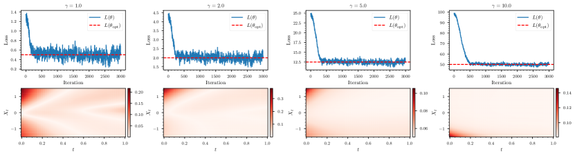
Figure 9: Results of Brownian bridges under different $\gamma$. Top row: the training loss log, the red dashed line represents the lower bound of $L(\theta)$.

Suppose $\gamma=\sigma=1.0$ and $x_{0}=v=0$. Figure 1 shows the empirical marginal distributions of $X^{\star}$ and $X^{\bullet}$ derived from independent samples from approximations of Equation (22) and Equation (23). In the topleft plot of Figure 9 we show how the training varies over iterations. The horizontal red line is the known lower bound on the training loss. In the bottomleft plot, we show a heatmap of the difference between the learned neural network and $\vartheta_{\theta_{\text{opt}}}$. The experiment has been repeated for other values of $\gamma$ ($2$, $5$ and $10$).

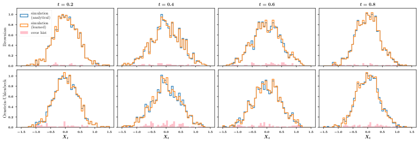
Figure 1: Comparison of marginal distributions at different time slices of the learned neural bridge and analytical true bridge. Top: Brownian bridges; Bottom: Ornstein-Uhlenbeck bridge, the pink bars show the error of each bin. The histograms are made from 1,000 independent trajectory samples individually.

We conclude that the neural net is able to learn the optimal drift and that the neural guided bridge is very close to the true bridge in terms of Kullback-Leibler divergence.

Ornstein-Uhlenbeck bridge: Consider the Ornstein-Uhlenbeck (OU) process

$$\mathrm{d}X_{t}=-\gamma X_{t}\mathrm{d}t+\sigma\mathrm{d}W_{t}.$$ (24)

Upon choosing $\tilde{X}_{t}=\sigma W_{t}$, the neural guided bridge satisfies the SDE

$$\mathrm{d}X^{\bullet}_{t}=\left\{-\gamma X^{\bullet}_{t}+\frac{v-X^{\bullet}_{t}}{T-t}+\sigma\vartheta_{\theta}(t,X^{\bullet}_{t})\right\}\mathrm{d}t+\sigma\mathrm{d}W_{t}.$$ (25)

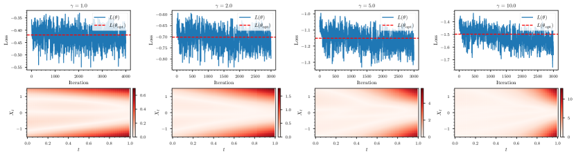
Figure 10: Results of Ornstein-Uhlenbeck bridges under different $\gamma$. Top row: the training loss log, the red dashed line represents the lower bound of $L(\theta)$.

In Appendix B.2 we derive the optimal map $\vartheta_{\theta_{\text{opt}}}$ and lower bound on $L$. With SDE parameters set as $x_{0}=v=0$, $\sigma=1.0$, we repeat the experiments of evaluating training loss curves and outputs of the learned neural network, as were done for the Brownian bridge and show the results in Figure 10.

A comparison of the results from Brownian and OU bridges reveals significant fluctuations in the training loss curves, particularly pronounced in the OU bridges. These fluctuations arise from the Monte Carlo approximation of the expectation and the numerical discretization of the integral in the training loss. The Monte Carlo approximation is implemented by computing the empirical mean over $N$ Wiener sample paths, while the integral is discretized on a finite grid $\mathcal{T}$ using left-point Riemann sums. The sampling introduces noise into the optimization, resulting in strong fluctuations. The discretization may cause bias in attaining the lower bound. In the OU case, $\vartheta_{\theta}$ exhibits a more complex form compared to the Brownian case, necessitating a finer grid and a larger number of Monte Carlo samples.

Despite the fluctuations observed during the training of the neural bridge, its validity under appropriate conditions is confirmed by quantitative evaluations in linear process experiments. For experiments lacking analytical references, performance is assessed qualitatively

5.2 Cell diffusion model

Wang et al. [2011] introduced a model for cell differentiation which serves as a test case for diffusion bridge simulation in Heng et al. [2022], Baker et al. [2024b]. Cellular expression levels $X_{t}=(X_{t,1},X_{t,2})$ are governed by the 2-dimensional SDE

$$\mathrm{d}X_{t}=\begin{bmatrix}\frac{X_{t,1}^{4}}{2^{-4}+X_{t,1}^{4}}+\frac{2^{-4}}{2^{-4}+X_{t,2}^{4}}-X_{t,1}\\ \frac{X_{t,2}^{4}}{2^{-4}+X_{t,2}^{4}}+\frac{2^{-4}}{2^{-4}+X_{t,1}^{4}}-X_{t,2}\end{bmatrix}\mathrm{d}t+\sigma\mathrm{d}W_{t},$$ (26)

driven by a 2-dimensional Wiener process $W$. The highly nonlinear drift makes this a challenging case. The guided neural bridge is constructed by taking the auxiliary process that drops the nonlinearities in the drift. More precisely,

$$\mathrm{d}\tilde{X}_{t}=-\tilde{X}_{t}\mathrm{d}t+\sigma\mathrm{d}W_{t}.$$ (27)

We study three representative cases that result in distinct dynamics for the conditional processes: (1) events that are likely under the forward process, which we refer to as “normal” events; (2) rare events; and (3) events that cause trajectories to exhibit multiple modes, where the marginal probability at certain times is multimodal. We compare our method to (a) the guided proposal [Schauer et al., 2017]; (b) bridge simulation via score matching [Heng et al., 2022]; and (c) bridge simulation using adjoint processes [Baker et al., 2024b]. Details of the experiments are presented in Appendix B.3.

Normal event: We set $x_{0}=[0.1,-0.1]^{T}$ and $v=[2.0,0.1]^{T}$. From multiple forward simulations, it can be assessed that balls around $v$ get non-negligible mass. We take $T=4.0$ and $\sigma=0.1$. In Figure 2, we show 30 conditional sample paths obtained by the three baseline methods mentioned above and the trained neural bridge. Since the true conditional process is analytically intractable, we sample 100,000 times from the forward (unconditional) process Equation (26) and retain samples that satisfy $\|LX_{T}-v\|\leq 0.01$. The obtained samples can be treated as a reference template for the true conditioned dynamics. Overall, all four methods successfully recover the truth dynamics. The performance of all four methods considered is comparable. We only note that the adjoint bridge sample paths appear slightly more dispersed.

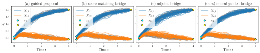
Figure 2: Visualization of 30 simulated bridges when conditioning on normal events using different methods. Note that except for the guided proposal, all the samples are independently drawn. The underlying grey trajectories presented in the figure are the unconditional samples by forward solving $X$ without conditioning and filtered by $\|LX_{T}-v\|<0.01$ as the reference of the true dynamics.

Rare event: We set $x_{0}=[0.1,-0.1]^{T}$, $v=[1.0,-0.1]^{T}$, which is a rare event for $X$ to hit. In this experiment, we set $\sigma=0.1$. Unlike the normal event case, the true dynamics cannot be recovered by brute-force sampling from the unconditioned process, as it is highly improbable that paths end up in a small ball around $v$. We display 30 conditional paths each generated by the four methods considered in Figure 3. Visual similarity can be observed between the neural guided bridge and the guided proposal, while the adjoint bridge cannot effectively model reasonable dynamics, as also reported in Baker et al. [2024b]. Score matching performs worst in this setting, which is expected because the score is learned from unconditional samples which as time $T$ tend to be far from $v$. This scarcity leads to poor estimation in those areas, resulting in significant deviations in the initial stages.

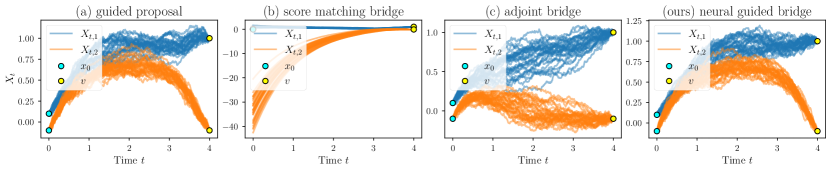
Figure 3: Visualization of 30 simulated bridges when conditioning on rare events using different methods. Note that except for the guided proposal, all the samples are independently drawn. No reference trajectory is available when conditioned on rare events.

Multi-modality: In both of the previous cases, each component’s marginal distribution at times $(0,T]$ is unimodal. However, with some special initial conditions, multimodality can arise, which poses a challenging task where one would like to recover all modes. Specifically, let $x_{0}=[-1.0,-1.0]^{T}$, $v=[-1.0,-1.0]^{T}$, $T=5.0$ and $\sigma=0.1$. Figure 4 compares the performance of the different methods. Both the adjoint bridge and score matching fail to model the dynamics accurately. The neural guided bridge and the guided proposal have comparable performance, as they both can only cover part of the modes. Moreover, when running pCN for a single chain, sometimes iterates of samples get stuck at a single mode. To address this, multiple chains must be run, which may become computationally expensive. In contrast, once the neural bridge is trained, new samples can be immediately generated by sampling paths from the learned SDE, at a cost comparable to unconditional forward simulation, while still covering the majority of modes.

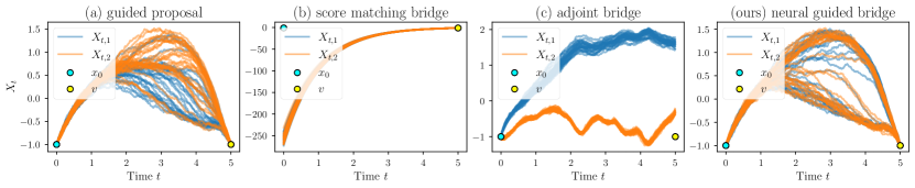
Figure 4: Visualization of 30 simulated bridges when conditioning on events that will cause multi-modality using different methods. Note that except for the guided proposal, all the samples are independently drawn. No reference trajectory is available when conditioned on multi-modality events.

Among all three tasks, our method demonstrates strong flexibility and adaptability, while the alternative methods show limitations when applied to specific tasks.

5.3 FitzHugh-Nagumo model

We consider a FitzHugh-Nagumo model, which is a prototype of an excitable system, considered for example in Ditlevsen and Samson [2019], Bierkens et al. [2020]. It is described by the SDE

$$\mathrm{d}X_{t}=\left\{\begin{bmatrix}\frac{1}{\chi}&-\frac{1}{\chi}\\ \gamma&-1\end{bmatrix}X_{t}+\begin{bmatrix}\frac{s-X^{3}_{t,1}}{\chi}\\ \alpha\end{bmatrix}\right\}\mathrm{d}t+\begin{bmatrix}0\\ \sigma\end{bmatrix}\mathrm{d}W_{t}$$ (28)

We condition the process by the value of its first component by setting $L=\begin{bmatrix}1&0\end{bmatrix}$ and hence condition on the event $LX_{T}=v$. We construct the guided proposal just as proposed in Bierkens et al. [2020] using the Taylor expansion $-x^{3}\approx 2v^{3}-3v^{2}x$ at $x=v$. Accordingly, we choose $\tilde{X}$

$$\mathrm{d}\tilde{X}_{t}=\left\{\begin{bmatrix}\frac{1-3v^{3}}{\chi}&-\frac{1}{\chi}\\ \gamma&-1\end{bmatrix}\tilde{X}_{t}+\begin{bmatrix}\frac{2v^{3}+s}{\chi}\\ \alpha\end{bmatrix}\right\}\mathrm{d}t+\begin{bmatrix}0\\ \sigma\end{bmatrix}\mathrm{d}W_{t}$$ (29)

Suppose $[\chi,s,\gamma,\alpha,\sigma]=[0.1,0,1.5,0.8,0.3]$. We examine the conditional behaviour of $X$ within $t\in[0,2.0]$ under two scenarios: (1) conditioning on a normal event $v=[-1.0]$; and (2) conditioning on a rare event $v=[1.1]$. As the score-matching and adjoint-process methods have not been proposed in the setting of a partially observed state, we only compare our method to the guided proposal. The results are shown in Figure 5 and Figure 6 respectively.

Normal event: Both the neural guided bridge and the guided proposal recover most patterns of the true process as shown in Figure 5. However, the neural guided bridge performs slightly better in capturing a broader spanning region of $X_{t,2}$ for $t\in(0.5,1.5)$. Additionally, $X_{t,1}$ generated by the neural guided bridge exhibits better visual consistency with the reference compared to the guided proposal.

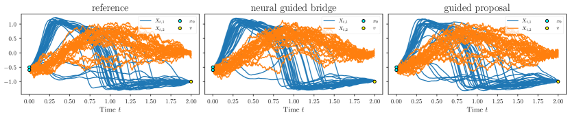
Figure 5: Visualization of FHN model conditioned on a normal event using 30 samples each either by drawing independently from the neural guided bridge or subsampling from the guided proposal updating history, the reference is obtained by directly sampling original Equation (28), and filtered by the condition $\|LX_{T}-v\|\leq 0.01$.

Rare event: The conditioning process introduces multimodality into the bridge, causing both methods to occasionally sample from only a single mode, as anticipated based on the previous example.

The left-hand panel of Figure 6 shows “true” conditioned paths obtained by forward sampling and keeping that paths that satisfy a relaxed version of the conditioning. Clearly, the bridge process is bimodal. The neural guided bridge samples paths from only one of the two modes, though the sampled paths appear very similar to the actual conditioned paths. The guided proposal samples paths inbetween the two modes as well, which are not seen in the reference panel. These observations suggest that both methods struggle to recover the 2 modes.

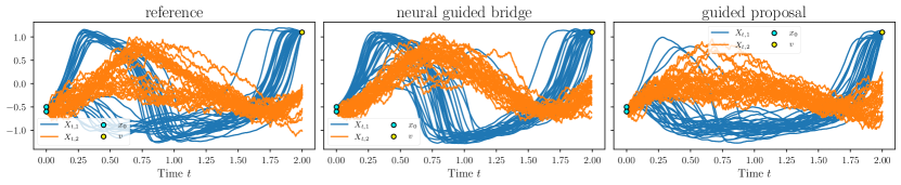
Figure 6: Visualization of FHN model conditioned on a rare event using 30 samples each either by drawing independently from the neural guided bridge or subsampling from the guided proposal updating history, the reference is obtained by directly sampling original Equation (28), and filtered by the condition $\|LX_{T}-v\|\leq 0.01$.

5.4 Stochastic landmark matching

At last, we consider a relatively high-dimensional stochastic nonlinear conditioning task: stochastic landmark matching, mainly specified in [Arnaudon et al., 2022], where a geometric shape is discretized and represented as $X_{t}=\{X^{(i)}_{t}\}_{i=1,\dots,n}\subset\mathbb{R}^{nd}$ a finite set of $n$ distinct landmarks $X^{(i)}_{t}\in D\subseteq\mathbb{R}^{d}$ and $d=\{2,3\}$ generally indicates a 2 or 3-dimensional shape. The stochastic landmark model defined in [Arnaudon et al., 2022] without momentum (i.e., only the coordinate variable dynamics) is defined by an SDE with a set of $n$ $d$-dimensional Wiener processes $W_{t}=\{W_{t}^{(j)}\}_{j=1,\dots,n}\in\mathbb{R}^{nd}$:

$$\mathrm{d}X_{t}=Q(X_{t})\mathrm{d}W_{t},\quad Q(X_{t})_{ij}\coloneq k(X_{t}^{(i)},X_{t}^{(j)}).$$ (30)

$k$ is a kernel function $\mathbb{R}^{d}\times\mathbb{R}^{d}\to\mathbb{R}$. We choose a Gaussian kernel $k(x,y)=\alpha\exp\left(-\frac{\|x-y\|^{2}}{2\kappa^{2}}\right)$. Note that the diffusion coefficient $Q$ is state-dependent, which is necessary for maintaining the structure of the shape during the evolution. Figure 13 shows an intuitive comparison between using a linear process and Equation (30) to model the stochastic evolutions of the same shape. In modelling real-world stochastic shapes like medical anatomical markers or biological species outlines, such a structure-preserving property of Equation 30 is preferred.

We choose

$$\mathrm{d}\tilde{X}_{t}=Q(X_{T})\mathrm{d}W_{t}.$$ (31)

That is, we only evaluate the diffusion coefficient at the endpoint and keep it constant throughout the process. We choose one ellipse as the starting point and another ellipse as the endpoint of the bridge. Each ellipse is discretized as 50 landmarks, leading to the dimension of $X_{t}$ being 100. The kernel parameters are chosen to be $\alpha=0.3,\kappa=0.5$ to ensure a strong correlation between a wide range of landmarks. Let $T=1.0$. Figure 7 and Figure 8 show 4 samples of the learned neural guided bridge and the guided proposal. Both methods capture the correct dynamics and approach the target shape. Despite the visual comparison, there is no quantitative way of comparing the performance of the two methods as the true bridge is anyway intractable. However, we note that for such a high-dimensional problem, using the Metropolis-Hasting method to sample from the guided proposal is much slower than numerical solving the trained neural guided bridge, since the latter only requires a single forward solving, while the former requires computationally expensive MCMC update steps, especially when the dimension of the problem is high. In this case, training a neural bridge once and subsequently generating independent samples may be preferable.

Figure 7: Four independent samples of the stochastic bridges between two ellipses obtained by solving the learned neural diffusion bridge. The target ellipse is marked in yellow, and the colour of the trajectories indicates time.

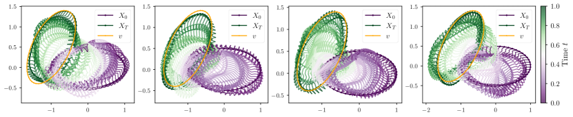
Figure 8: Four samples of the stochastic bridges between two ellipses obtained by subsampling from the guided proposal updating history. The target ellipse is marked in yellow, and the colour of the trajectories indicates time.

6 Conclusions and limitations

We propose the neural guided diffusion bridge, a novel method for simulating diffusion bridges that enhances guided proposals through variational inference, eliminating the need for MCMC or SMC. This approach enables efficient independent sampling with comparable quality in challenging tasks where existing score-learning-based methods struggle. Extensive experiments, including both quantitative and qualitative evaluations, validate the effectiveness of our method. However, as the framework is formulated variationally and optimized by minimizing $\mathrm{D_{KL}}{(\mathbb{P}^{\bullet}_{\theta}||\mathbb{P}^{\star})}$, it exhibits mode-seeking behaviour, potentially limiting its ability to explore all modes compared to running multiple MCMC chains. Despite this limitation, our method provides a computationally efficient alternative to guided proposals, particularly in generating independent conditioned samples.

Our approach focuses on better approximating the drift of the conditioned process while keeping the guiding term that ensures the process hits $v$ at time $T$ relatively simple. In future work, one could try to jointly learn $\vartheta_{\theta}$ and $B$ using variational inference. Another venue of future research can be to extend our approach to conditioning on partial observations at multiple future times.

Appendix A Theoretical details

A.1 Preconditioned Crank-Nicolson

A more general version of using pCN to sample $X^{\star}$ is illustrated in Mider et al. [2021, Section 4], where multiples states can be observed at times $0=t_{0}<t_{1}<\dots<t_{n}$, while in our case, we suppose only the endpoint state is observed, leading to a simpler version of Mider et al. [2021, Algorithm 4.1], as Algorithm 2.

Algorithm 2 Preconditioned Crank-Nicolson

1:Input: Discrete time grid $\mathcal{T}:=\{t_{m}\}_{m=0,1,\dots,M}$, tuning parameter $\eta\in[0,1)$, number of required samples $K$

2:Solve Equation (12) on $\mathcal{T}$, obtain $\{\tilde{H}(t_{m})\},\{\tilde{r}(t_{m},\cdot)\}$ using Equation (11).

3:Sample $w=\{w_{t_{m}}\}$ on $\mathcal{T}$.

4:Solve Equation (6) on $\mathcal{T}$ with $w=\{w_{t_{m}}\}$, obtain $y=\{y_{t_{m}}\}$.

5:repeat

6:  Sample new innovations $z=\{z_{t_{m}}\}$ on $\mathcal{T}$ independently.

7:  Set $w^{\circ}=\eta w+\sqrt{1-\eta^{2}}z$.

8:  Solve Equation (6) on $\mathcal{T}$ with $z=\{z_{t_{m}}\}$, obtain $y^{\circ}=\{y^{\circ}_{t_{m}}\}$.

9:  Compute $A=\Psi(y^{\circ})/\Psi(y)$ with $\{y^{\circ}_{t_{m}}\}|$ and $\{y_{t_{m}}\}$ using Equation (10a).

10:  Draw $U\sim\mathcal{U}(0,1)$.

11:  if $U<A$ then

12:   $y\leftarrow y^{\circ}$ and $w\leftarrow w^{\circ}$

13:   Save $y$.

14:  end if

15:until Sample counts $>K$.

A.2 Proof of Theorem 2

Proof.

Consider the KL divergence between $\mathbb{P}^{\bullet}_{\theta}$ and $\mathbb{P}^{\star}$:

$$\mathrm{D}_{\text{KL}}{(\mathbb{P}^{\bullet}_{\theta}||\mathbb{P}^{\star})} =\mathbb{E}^{\bullet}\left[\log\left(\frac{\mathrm{d}\mathbb{L}^{\bullet}_{\theta}}{\mathrm{d}\mathbb{L}^{\star}}\right)(X)\right]$$

$$=\mathbb{E}^{\bullet}\left[\log\left(\frac{\mathrm{d}\mathbb{L}^{\bullet}_{\theta}}{\mathrm{d}\mathbb{L}^{\circ}}\cdot\frac{\mathrm{d}\mathbb{L}^{\circ}}{\mathrm{d}\mathbb{L}^{\star}}\right)(X)\right]$$

$$=\mathbb{E}^{\bullet}\left[\log\left(\frac{\mathrm{d}\mathbb{L}^{\bullet}_{\theta}}{\mathrm{d}\mathbb{L}^{\circ}}(X)\right)\right]-\mathbb{E}^{\bullet}\left[\log\left(\frac{\mathrm{d}\mathbb{L}^{\star}}{\mathrm{d}\mathbb{L}^{\circ}}(X)\right)\right].$$ (32a)

By Girsanov’s theorem,

$$\mathbb{E}^{\bullet}\left[\log\left(\frac{\mathrm{d}\mathbb{L}^{\bullet}_{\theta}}{\mathrm{d}\mathbb{L}^{\circ}}(X)\right)\right] =\mathbb{E}^{\bullet}\left[\log\frac{\mathrm{d}\mathbb{P}^{\bullet}_{\theta}}{\mathrm{d}\mathbb{P}^{\circ}}\right]$$ (33a)

$$=\mathbb{E}^{\bullet}\left[\int_{0}^{T}\vartheta_{\theta}(t,X_{t})\mathrm{d}W^{\circ}_{t}-\frac{1}{2}\int_{0}^{T}\|\vartheta_{\theta}(t,X_{t})\|^{2}\mathrm{d}t\right]$$

$$=\mathbb{E}^{\bullet}\left[\int_{0}^{T}\vartheta_{\theta}(t,X_{t})\mathrm{d}W_{t}^{\bullet}+\frac{1}{2}\int_{0}^{T}\|\vartheta_{\theta}(t,X_{t})\|^{2}\mathrm{d}t\right]$$

$$=\mathbb{E}^{\bullet}\left[\frac{1}{2}\int_{0}^{T}\|\vartheta_{\theta}(t,X_{t})\|^{2}\mathrm{d}t\right],$$ (33b)

where the stochastic integral vanishes because of the martingale property of the Itô integral. The first equality follows from Equation (14). By Equation (7)

$$\mathbb{E}^{\bullet}\left[\log\left(\frac{\mathrm{d}\mathbb{L}^{\star}}{\mathrm{d}\mathbb{L}^{\circ}}(X)\right)\right]=\mathbb{E}^{\bullet}\left[\int_{0}^{T}G(t,X_{t})\mathrm{d}t\right]+\log\frac{\tilde{h}(0,x_{0})}{h(0,x_{0})}.$$ (34)

Substituting Equation (33b) and Equation (34) into Equation (32a) gives

$$\mathrm{D}_{\text{KL}}{(\mathbb{P}^{\bullet}_{\theta}||\mathbb{P}^{\star})}=\mathbb{E}^{\bullet}\int_{0}^{T}\left\{\frac{1}{2}\|\vartheta_{\theta}(t,X_{t})\|^{2}-G(t,X_{t})\right\}\mathrm{d}t+\log\frac{\tilde{h}(0,x_{0})}{h(0,x_{0})}=L(\theta)+\log\frac{\tilde{h}(0,x_{0})}{h(0,x_{0})}\geq 0,$$ (35)

as $L(\theta)$ defined as Equation (18). ∎

A.3 SDE gradients

We now derive the gradient of Equation (21) with respect to $\theta$, on a fixed Wiener realization $w^{\bullet(n)}=\{w^{\bullet(n)}_{t_{m}}\}$. As discussed, $x^{\bullet(n)}_{t_{m}}=\phi_{\theta}(w^{\bullet(n)}_{t_{m}})$ is implemented as a numerical SDE solver $f_{\theta}(w^{\bullet(n)}_{t_{m}},t_{m-1},x^{\bullet(n)}_{t_{m-1}}),m\geq 1$ that takes the previous step $(t_{m-1},x^{\bullet(n)}_{t_{m-1}})$ as additional arguments. As $x^{\bullet(n)}_{t_{m-1}}$ also depends on $\theta$, the gradient with respect to $\theta$ needs to be computed recursively. Specifically, with $x^{\bullet(n)}_{t_{m}}=f_{\theta,m}=f_{\theta}(w^{\bullet(n)}_{t_{m}},t_{m-1},x^{\bullet(n)}_{t_{m-1}})$

$$\nabla_{\theta}\left(\frac{1}{2}\|\vartheta_{\theta}(t_{m-1},\phi_{\theta}(w^{\bullet(n)}_{t_{m-1}})\|^{2}_{2}\right)=\nabla_{\theta}\left(\frac{1}{2}\|\vartheta_{\theta}(t_{m-1},f_{\theta,m-1})\|^{2}_{2}\right)$$ (36a)

$$=[\nabla_{\theta}\vartheta_{\theta}(t_{m-1},f_{\theta,m-1}))]^{T}\vartheta_{\theta}(t_{m-1},f_{\theta,m-1})$$ (36b)

$$=\left[\frac{\partial\vartheta_{\theta}(t_{m-1},f_{\theta,m-1})}{\partial\theta}+\frac{\partial\vartheta_{\theta}(t_{m-1},f_{\theta,m-1})}{\partial f_{\theta,m-1}}\cdot\nabla_{\theta}f_{\theta,m-1}\right]^{T}\vartheta_{\theta}(t_{m-1},f_{\theta,m-1})$$ (36c)

$$=\left[\frac{\partial\vartheta_{\theta}(t_{m-1},f_{\theta,m-1})}{\partial\theta}+\frac{\partial\vartheta_{\theta}(t_{m-1},f_{\theta,m-1})}{\partial f_{\theta,m-1}}\cdot\left(\frac{\partial f_{\theta,m-1}}{\partial\theta}+\frac{\partial f_{\theta,m-1}}{\partial f_{\theta,m-2}}\cdot\nabla_{\theta}f_{\theta,m-2}\right)\right]^{T}\vartheta_{\theta}(t_{m-1},f_{\theta,m-1})$$ (36d)

$$=\left[\frac{\partial\vartheta_{\theta}(t_{m-1},f_{\theta,m-1})}{\partial\theta}+\frac{\partial\vartheta_{\theta}(t_{m-1},f_{\theta,m-1})}{\partial f_{\theta,m-1}}\cdot\left(\frac{\partial f_{\theta,m-1}}{\partial\theta}+\sum^{m-2}_{i=1}\left(\prod^{m-1}_{j=i+1}\frac{\partial f_{\theta,j}}{\partial f_{\theta,j-1}}{}\right)\frac{\partial f_{\theta,i}}{\partial\theta}\right)\right]^{T}\vartheta_{\theta}(t_{m-1},f_{\theta,m-1}),$$ (36e)

Similiarly, the gradient of $G$ with respect to $\theta$ can also be computed recusively:

$$\nabla_{\theta}G(t_{m-1},\phi_{\theta}(w^{\bullet(n)}_{t_{m-1}}))=\frac{\partial G(t_{m-1},f_{\theta,m-1})}{\partial f_{\theta,m-1}}\cdot\left(\frac{\partial f_{\theta,m-1}}{\partial\theta}+\sum^{m-2}_{i=1}\left(\prod^{m-1}_{j=i+1}\frac{\partial f_{\theta,j}}{\partial f_{\theta,j-1}}\right)\frac{\partial f_{\theta,i}}{\partial\theta}\right).$$ (37)

The gradient of $L(\theta)$ can be approximated by:

$$\nabla_{\theta}L(\theta)\approx\frac{1}{N}\sum^{N}_{n=1}\sum^{M}_{m=1}\left\{\nabla_{\theta}\left(\frac{1}{2}\|\vartheta_{\theta}(t_{m-1},\phi_{\theta}(w^{\bullet(n)}_{t_{m-1}}))\|^{2}_{2}\right)-\nabla_{\theta}G(t_{m-1},\phi_{\theta}(w^{\bullet(n)}_{t_{m-1}}))\right\}\delta t.$$ (38)

The realization of $f_{\theta}$ depends on the chosen numerical integrator. We choose Euler-Maruyama as the integrator used for all the experiments conducted in Section 5. Under this scheme, $f_{\theta}$ is:

$$f_{\theta}(w^{\bullet(n)}_{t_{m}},t_{m-1},x^{\bullet(n)}_{t_{m-1}})=x^{\bullet(n)}_{t_{m-1}}+(b+a\tilde{r}+\sigma\vartheta_{\theta})(t_{m-1},x^{\bullet(n)}_{t_{m-1}})+\sigma(t_{m-1},x^{\bullet(n)}_{t_{m-1}})w^{\bullet(n)}_{t_{m}},$$ (39)

with $w^{\bullet(n)}_{t_{m}}\sim\mathcal{N}(0,(t_{m}-t_{m-1})\mathbf{I}_{d})$. The derivatives can be computed accordingly:

$$\frac{\partial f_{\theta,m}}{\partial\theta} =\sigma(t_{m-1},x^{\bullet(n)}_{t_{m-1}})\frac{\partial\vartheta_{\theta}(t_{m-1},x^{\bullet(n)}_{t_{m-1}})}{\partial\theta}$$ (40a)

$$\frac{\partial f_{\theta,m}}{\partial f_{\theta,m-1}} =1+\frac{\partial(b+a\tilde{r}+\sigma\vartheta_{\theta})}{\partial x^{\bullet(n)}_{t_{m-1}}}(t_{m-1},x^{\bullet(n)}_{t_{m-1}})+\frac{\partial\sigma}{\partial x^{\bullet(n)}_{t_{m-1}}}(t_{m-1},x^{\bullet(n)}_{t_{m-1}})w^{\bullet(n)}_{t_{m}}.$$ (40b)

The automatic differentiation can save all the intermediate Equation (40a) and Equation (40b), which enables to compute $\nabla_{\theta}L(\theta)$.

Appendix B Experiment details

B.1 Code implementation

The codebase for reproducing all the experiments conducted in the paper is available in https://github.com/bookdiver/neuralbridge

B.2 Linear processes

Brownian bridges: When no noise is in observations, $h(0,x_{0})=\mathcal{N}(y;x-\gamma T,\sigma^{2}T)$, $\tilde{h}(0,x_{0})=\mathcal{N}(y;x,\sigma^{2}T)$, therefore, the lower bound of $L(\theta)$, $-\log\frac{\tilde{h}(0,x_{0})}{h(0,x_{0})}=(\|y-x_{0}-\gamma T\|^{2}-\|y-x_{0}\|^{2})/(2\sigma^{2}T)$. In practice, we set $\epsilon=10^{-10}$, $\vartheta_{\theta}(t,x)$ is modelled as a fully-connected neural network with 3 hidden layers and 20 hidden dimensions for each layer. The model is trained with 60,000 independently sampled full trajectories of $X^{\bullet}_{t}$. The batch size $N=20$, time step size $\delta t=0.005$, therefore in total $M=200$ time steps. The network is trained with Adam [Kingma and Ba, 2017] optimizer with an initial learning rate of $1.0e^{-3}$ and a cosine decay scheduler, and a linear learning rate warming up in the first 0.1 ratio of training iterations.

Ornstein-Uhlenbeck bridge: When conditioning Equation (24) on $\{LX_{T}=v\}$, the conditioned process $X^{\star}$ reads:

$$\mathrm{d}X^{\star}_{t}=-\gamma\left(\frac{v}{\operatorname{sinh}(-\gamma(T-t))}-\frac{x}{\operatorname{tanh}(-\gamma(T-t))}\right)\mathrm{d}t+\sigma\mathrm{d}W_{t},$$ (41)

which is obtained from the fact that

$$p(T,y\mid t,x)=\sqrt{\frac{\gamma}{\pi\sigma^{2}(1-\exp(-2\gamma(T-t))}}\exp\left\{-\frac{\gamma}{\sigma^{2}}\cdot\frac{(y-x\exp(-\gamma(T-t))^{2}}{1-\exp(-2\gamma(T-t))}\right\}.$$ (42)

Therefore, one can immediately see the optimal value of $\vartheta_{\theta}(t,x)$ to be

$$\vartheta_{\theta_{\text{opt}}}(t,x)=\frac{1}{\sigma}\left\{-\gamma\left[\frac{v}{\sinh(-\gamma(T-t))}-\frac{x}{\tanh(-\gamma(T-t))}\right]-\frac{v-x}{T-t}+\gamma\cdot x\right\},$$ (43)

and the lower bound of $L(\theta)$ to be:

$$-\log\frac{\tilde{h}(0,x_{0})}{h(0,x_{0})}=\frac{1}{2}\left\{\log\left(\frac{\gamma}{\pi\sigma^{2}(1-e^{-2\gamma T})}\right)-\frac{\gamma(y-x_{0}e^{-\gamma T})^{2}}{\sigma^{2}(1-e^{-2\gamma T})}-\log\left(\frac{1}{2\pi\sigma^{2}T}\right)+\frac{(y-x_{0})^{2}}{\sigma^{2}T}\right\}.$$ (44)

These analytical results enable a quantitative evaluation of the performance of learned $X^{\bullet}$. The training setups are duplicated from the previous Brownian bridges, except for a deeper neural network architecture with 4 hidden layers and 20 hidden units in each layer.

B.3 Cell diffusion process

For the benchmark tests, we adapt the published implementations of the corresponding methods to fit into our test framework with possibly minor modifications. Specifically, the original guided proposal codebase is implemented with Julia in , we rewrite it in JAX [Bradbury et al., 2018]; the score matching bridge repository is published in , which is written with PyTorch [Paszke et al., 2019], we also adapt it into JAX for convenience, additionally, as also reported by the authors, Heng et al. [2022] introduces two score-matching-based bridge simulation schemes, reversed and forward simulation, and the forward simulation relies on the reversed simulation, and learning from approximated reversed bridge can magnifies the errors due to progressive accumulation. Therefore, we only compare our method with the reversed bridge learning to avoid error accumulations; the adjoint bridge is implemented in , already in JAX, so we directly use the existing implementation without modification.

Normal event: We still consider a no-observation-noise case by setting $\epsilon=10^{-10}$, $\vartheta_{\theta}$ is modelled as a fully-connected network with 4 hidden layers and 32 hidden dimensions per layer, activated by tanh. We train the model with 100,000 independent samples of $X^{\bullet}$ by a Adam optimizor with initial learning rate of $5e^{-4}$, batch size $N=20$, time step $\delta t=0.01$, therefore, in total $M=400$ time steps. For the guided proposal, we set $\eta=0.98$, and run one chain of MCMC for 10,000 updates, obtaining $22.69\%$ acceptance rate. The burn-in period is set as the first 4,000 steps. After burn-in, we subsample the updating history by taking every 200-th sample, therefore selecting out 30 samples. In the following experiments, if not explicitly stated, all the samples from the guided proposal are similarly obtained from one chain of MCMC by taking proper thinning ratios. For the score matching, we find the original neural network architecture in the repository performs poorly in our case, so we refer to the architecture used in Baker et al. [2024a], with 4 hidden layers and 32 hidden dimensions per layer, combining with the sinusoidal embedding [Vaswani et al., 2017] for the temporal dependency. For the adjoint bridge, we directly deploy the original architecture used in Baker et al. [2024b]. To obtain the reference dynamics, we generate 100,000 independent samples of $X$, then filter these by the condition $\|LX_{T}-v\|\leq 0.01$, obtaining 151 valid samples, and only the first 30 samples are shown in grey.

Rare event: The setups for conditioning on rare events of the neural guided bridge are replicated from the previous normal event case, except for the MCMC is running with sightly increased tuning parameter $\eta=0.99$ and obtains an acceptance rate of $24.50\%$. For the score matching bridge, since we only use the reversed bridge, whose learning is independent of the endpoints, we directly deploy the trained score approximation from the previous case; For the adjoint process, we fix the neural network architecture and training scheme, changing only the conditions. To obtain the reference, we repeat the same procedure of sampling 100,000 independent trajectories and filtering by the condition, however, we find none of the samples matches the condition we put, which reflects that $v=[1.0,-0.1]^{T}$ is indeed a probably rare event and becomes challenging.

Multi-modality: All the neural network architectures and training schemes are the same as in previous examples. $\delta t=0.01$ and $M=500$ therefore. For the guided proposal, we run one chain for 10,000 iterations with $\eta=0.9$, obtaining $24.93\%$ acceptance rate. Similarly to the rare event case, no valid samples can be found through 100,000 brute-forced samples of the original process. Figure 11 shows marginal distributions of the original and conditioned processes, where more than one peak of marginal distribution density can be observed at time $t=3.0,4.0$. Neither the neural guided process nor the guided proposal can recover all three modes which are indicated by the original process. However, one can always run multiple independent chains to cover all the modes, as suggested in Figure 12. Compared to the guided proposal, even though the neural bridge can not recover all the modes, it trades with fast sample speed. Also, additional MCMC updates can be further executed on trained neural bridges to obtain high-quality samples.

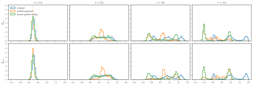
Figure 11: Comparison of marginal distributions at different time slices of the original process, guided proposal and learned neural bridge. The histograms are made from 1,000 samples individually either drawn independently from the neural guided bridge and original process or subsampled from the guided proposal updating history. Top row: the first component of $X$; Bottom row: the second component of $X$.

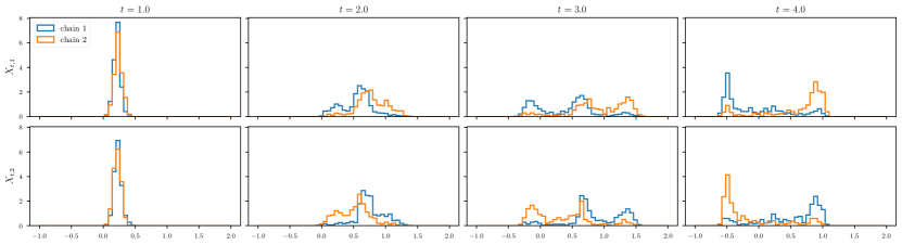
Figure 12: Marginal distributions of two independent MCMC chains, where they compensate each other and cover all three modes.

B.4 FitzHugh-Nagumo model

Normal event: We set $\delta t=0.005$, which leads to $N=400$ time steps. The observation noise variance is $\epsilon=1e-4$ to ensure a stable backward filtering ODE solution. For the neural guided bridge, $\vartheta_{\theta}(t,x)$ is constructed as a fully connected neural network with 4 hidden layers and 32 hidden dimensions at each layer, activated by tanh functions. The training is done with 225,000 independent samples from $X^{\bullet}_{t}$, batch size $M=30$, optimized by Adam with an initial learning rate of $5e-4$ and a cosine decay scheduler. For the guided proposal, we set $\eta=0$ as suggested in Bierkens et al. [2020] and run one chain for 50,000 iterations with a burn-in of 20,000 steps, obtaining $61.15\%$ acceptance rate. The reference is obtained by brutal-forced sampling $X$ 100,000 times and applying the filtering, which obtain 4814 valid samples, only the first 30 are shown in the figure.

Rare event: We use the same time step size as the previous experiment, however, a quadratic transformation $\tau(t)=t(2-t/T)$ is deployed to get an irregular grid, where the closer to the endpoint $T$, the denser the grid. The observation noise variance is $\epsilon=2e-4$. $\vartheta_{\theta}(t,x)$ architecture is the same, but training for a longer time with 300,000 independent samples. For the guided proposal, $\eta=0.9$, it runs one chain for 20,000 iterations with a burn-in period as the first 2,000 steps and obtains $23.18\%$ acceptance rate. Another notable thing is to obtain the reference by brutal forced sampling, one can only get 104 ($1.04$ ‰) samples that meet the rare conditionals out of 100,000 forward samplings, while in the normal case, the number of valid samples is 4814 ($4.81\%$).

B.5 Stochastic landmark matching

To demonstrate the necessity of using a state-dependent nonlinear process as Equation (30) to model the shape process rather than a linear one with a fixed diffusion matrix, we show a comparison of forward processes under two scenarios as Figure 13, where the linear process is similar to the auxiliary process Equation (31), but with a fixed $Q$ evaluated at the starting point $x_{0}$, except for the evaluation point, the rest parameters for the kernel are the same. In Equation (30), as $X_{t}^{(j)}$ approaching $X_{t}^{(i)}$, the correlation between them becomes stronger, which forces them to move synchronically, thus preventing the overlapping and intersection. Also, when $\kappa\to 0$, the process defined by Equation (30) will degenerate to Brownian motion.

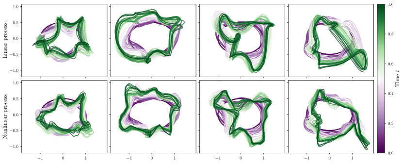
Figure 13: Comparison of using a linear (Top row) with a fixed diffusion coefficient and Equation (30) (Bottom row) to model the stochastic evolution of an ellipse shape (marked in purple) using 4 different samples of trajectories individually, where the nonlinear Equation (30) preserves the topology of the ellipse, which is broken during the evolution under the linear process.

The observation noise variance is set as $\epsilon=2e-3$, as we find too small values of $\epsilon$ will cause numerical instability. We deploy the neural network architecture suggested in Heng et al. [2022] to model $\vartheta_{\theta}$, whose encoding part is a two-layer MLP with 128 hidden units at each layer, and the decoding part is a three-layer MLP with hidden units of 256, 256, and 128 individually. The network is activated by tanh, and trained with 240,000 independent samples from $X^{\bullet}$ with batch size $N=8$, optimized by Adam with an initial learning rate of 7.0e-4 and a cosine decay scheduler. For the guided proposal, we run one chain for 5,000 iterations and drop the first 1,000 iterations as the burn-in, with $\eta=0.95$ and obtain $12.62\%$ acceptance rate on average.

References

- Zhou et al. [2024] Linqi Zhou, Aaron Lou, Samar Khanna, and Stefano Ermon. Denoising diffusion bridge models. In The Twelfth International Conference on Learning Representations, 2024. URL https://openreview.net/forum?id=FKksTayvGo.
- Zheng et al. [2024] Kaiwen Zheng, Guande He, Jianfei Chen, Fan Bao, and Jun Zhu. Diffusion bridge implicit models. arXiv preprint arXiv:2405.15885, 2024. URL http://arxiv.org/abs/2405.15885.
- Arnaudon et al. [2022] Alexis Arnaudon, Frank van der Meulen, Moritz Schauer, and Stefan Sommer. Diffusion bridges for stochastic hamiltonian systems and shape evolutions. SIAM Journal on Imaging Sciences, 15(1):293–323, March 2022. ISSN 1936-4954. doi: 10.1137/21M1406283. URL http://arxiv.org/abs/2002.00885.
- Baker et al. [2024a] Elizabeth Louise Baker, Gefan Yang, Michael Lind Severinsen, Christy Anna Hipsley, and Stefan Sommer. Conditioning non-linear and infinite-dimensional diffusion processes. In The Thirty-eighth Annual Conference on Neural Information Processing Systems, 2024a. URL https://openreview.net/forum?id=FV4an2OuFM.
- Yang et al. [2024] Gefan Yang, Elizabeth Louise Baker, Michael Lind Severinsen, Christy Anna Hipsley, and Stefan Sommer. Simulating infinite-dimensional nonlinear diffusion bridges. arXiv preprint arXiv:2405.18353, 2024. URL http://arxiv.org/abs/2405.18353.
- Delyon and Hu [2006] Bernard Delyon and Ying Hu. Simulation of conditioned diffusion and application to parameter estimation. Stochastic Processes and their Applications, 116(11):1660–1675, 2006.
- van der Meulen and Schauer [2017] Frank van der Meulen and Moritz Schauer. Bayesian estimation of discretely observed multi-dimensional diffusion processes using guided proposals. Electronic Journal of Statistics, 11(1), 2017. ISSN 1935-7524. doi: 10.1214/17-EJS1290.
- van der Meulen and Schauer [2018] Frank van der Meulen and Moritz Schauer. Bayesian estimation of incompletely observed diffusions. Stochastics, 90(5):641–662, 2018.
- Pieschner and Fuchs [2020] Susanne Pieschner and Christiane Fuchs. Bayesian inference for diffusion processes: using higher-order approximations for transition densities. Royal Society Open Science, 7(10):200270, 2020. ISSN 2054-5703. doi: 10.1098/rsos.200270.
- Rogers and Williams [2000] L Chris G Rogers and David Williams. Diffusions, Markov processes, and martingales: Itô calculus, volume 2. Cambridge university press, 2000.
- Beskos et al. [2006] Alexandros Beskos, Omiros Papaspiliopoulos, Gareth O. Roberts, and Paul Fearnhead. Exact and computationally efficient likelihood-based estimation for discretely observed diffusion processes. Journal of the Royal Statistical Society: Series B (Statistical Methodology), 68(3):333–382, 2006. ISSN 1467-9868. doi: 10.1111/j.1467-9868.2006.00552.x. URL https://onlinelibrary.wiley.com/doi/abs/10.1111/j.1467-9868.2006.00552.x.
- Schauer et al. [2017] Moritz Schauer, Frank van der Meulen, and Harry van Zanten. Guided proposals for simulating multi-dimensional diffusion bridges. Bernoulli, 23(4A), November 2017. ISSN 1350-7265. doi: 10.3150/16-BEJ833. URL http://arxiv.org/abs/1311.3606.
- Whitaker et al. [2016] Gavin A Whitaker, Andrew Golightly, Richard J Boys, and Chris Sherlock. Improved bridge constructs for stochastic differential equations. Statistics and Computing, 4(27):885–900, 2016.
- Bierkens et al. [2021] Joris Bierkens, Sebastiano Grazzi, Frank Van Der Meulen, and Moritz Schauer. A piecewise deterministic monte carlo method for diffusion bridges. Statistics and Computing, 31(3):37, 2021. ISSN 0960-3174, 1573-1375. doi: 10.1007/s11222-021-10008-8.
- Mider et al. [2021] Marcin Mider, Moritz Schauer, and Frank van der Meulen. Continuous-discrete smoothing of diffusions. Electronic Journal of Statistics, 15(2):4295 – 4342, 2021. doi: 10.1214/21-EJS1894. URL https://doi.org/10.1214/21-EJS1894.
- Heng et al. [2022] Jeremy Heng, Valentin De Bortoli, Arnaud Doucet, and James Thornton. Simulating diffusion bridges with score matching. arXiv preprint arXiv:2111.07243, 2022. URL http://arxiv.org/abs/2111.07243.
- Chau et al. [2024] H. Chau, J. L. Kirkby, D. H. Nguyen, D. Nguyen, N. Nguyen, and T. Nguyen. An efficient method to simulate diffusion bridges. Statistics and Computing, 34(4):131, 2024. ISSN 0960-3174, 1573-1375. doi: 10.1007/s11222-024-10439-z.
- Hyvarinen [2005] Aapo Hyvarinen. Estimation of non-normalized statistical models by score matching. Journal of Machine Learning Research, page 15, 2005.
- Vincent [2011] Pascal Vincent. A connection between score matching and denoising autoencoders. Neural Computation, 23(7):1661–1674, 2011. ISSN 0899-7667, 1530-888X. doi: 10.1162/NECO_a_00142.
- Baker et al. [2024b] Elizabeth Louise Baker, Moritz Schauer, and Stefan Sommer. Score matching for bridges without time-reversals. arXiv preprint arXiv:2407.15455, 2024b. URL http://arxiv.org/abs/1712.03807.
- Sommer et al. [2017] Stefan Sommer, Alexis Arnaudon, Line Kuhnel, and Sarang Joshi. Bridge simulation and metric estimation on landmark manifolds. arXiv preprint arXiv:1705.10943, 2017. URL http://arxiv.org/abs/1705.10943.
- Jensen and Sommer [2023] Mathias Højgaard Jensen and Stefan Sommer. Simulation of conditioned semimartingales on riemannian manifolds. arXiv preprint arXiv:2105.13190, 2023. URL http://arxiv.org/abs/2105.13190.
- Grong et al. [2024] Erlend Grong, Karen Habermann, and Stefan Sommer. Score matching for sub-riemannian bridge sampling. arXiv preprint arXiv:2404.15258, 2024. URL http://arxiv.org/abs/2404.15258.
- Corstanje et al. [2024] Marc Corstanje, Frank van der Meulen, Moritz Schauer, and Stefan Sommer. Simulating conditioned diffusions on manifolds. arXiv preprint arXiv:2403.05409, 2024. URL http://arxiv.org/abs/2403.05409.
- Cotter et al. [2013] S. L. Cotter, G. O. Roberts, A. M. Stuart, and D. White. Mcmc methods for functions: Modifying old algorithms to make them faster. Statistical Science, 28(3):424–446, 2013. ISSN 08834237, 21688745.
- Clark [1990] J.M.C. Clark. The simulation of pinned diffusions. In 29th IEEE Conference on Decision and Control, pages 1418–1420 vol.3, 1990. doi: 10.1109/CDC.1990.203845. URL https://ieeexplore.ieee.org/document/203845/?arnumber=203845.
- Chib et al. [2004] Siddhartha Chib, Michael K. Pitt, and Neil Shephard. Likelihood Based Inference for Diffusion Driven <odels. OFRC Working Papers Series 2004fe17, Oxford Financial Research Centre, 2004. URL https://ideas.repec.org/p/sbs/wpsefe/2004fe17.html.
- Lin et al. [2010] Ming Lin, Rong Chen, and Per Mykland. On generating monte carlo samples of continuous diffusion bridges. Journal of the American Statistical Association, 105(490):820–838, 2010.
- Golightly and Wilkinson [2010] Andrew Golightly and Darren J. Wilkinson. Learning and Inference in Computational Systems Biology. MIT Press, 2010.
- Bierkens et al. [2020] Joris Bierkens, Frank Van Der Meulen, and Moritz Schauer. Simulation of elliptic and hypo-elliptic conditional diffusions. Advances in Applied Probability, 52(1):173–212, 2020. ISSN 0001-8678, 1475-6064. doi: 10.1017/apr.2019.54.
- Thornton et al. [2022] James Thornton, Michael Hutchinson, Emile Mathieu, Valentin De Bortoli, Yee Whye Teh, and Arnaud Doucet. Riemannian diffusion schrödinger bridge. arXiv preprint arXiv:2207.03024, 2022. URL http://arxiv.org/abs/2207.03024.
- De Bortoli et al. [2021] Valentin De Bortoli, James Thornton, Jeremy Heng, and Arnaud Doucet. Diffusion schrödinger bridge with applications to score-based generative modeling. In Advances in Neural Information Processing Systems, volume 34, pages 17695–17709, 2021.
- Shi et al. [2024] Yuyang Shi, Valentin De Bortoli, Andrew Campbell, and Arnaud Doucet. Diffusion schrödinger bridge matching. In Advances in Neural Information Processing Systems, volume 36, 2024.
- Tang et al. [2024] Zhicong Tang, Tiankai Hang, Shuyang Gu, Dong Chen, and Baining Guo. Simplified diffusion schrödinger bridge. arXiv preprint arXiv:2403.14623, 2024. URL http://arxiv.org/abs/2403.14623.
- Chen et al. [2018] Ricky TQ Chen, Yulia Rubanova, Jesse Bettencourt, and David K Duvenaud. Neural ordinary differential equations. In Advances in neural information processing systems, volume 31, 2018.
- Tzen and Raginsky [2019a] Belinda Tzen and Maxim Raginsky. Neural stochastic differential equations: Deep latent gaussian models in the diffusion limit. arXiv preprint arXiv:1905.09883, 2019a. URL http://arxiv.org/abs/1905.09883.
- Tzen and Raginsky [2019b] Belinda Tzen and Maxim Raginsky. Theoretical guarantees for sampling and inference in generative models with latent diffusions. In Conference on Learning Theory, pages 3084–3114. PMLR, 2019b.
- Li et al. [2020] Xuechen Li, Ting-Kam Leonard Wong, Ricky TQ Chen, and David Duvenaud. Scalable gradients for stochastic differential equations. In International Conference on Artificial Intelligence and Statistics, pages 3870–3882. PMLR, 2020.
- Kidger et al. [2021] Patrick Kidger, James Foster, Xuechen Li, and Terry J Lyons. Neural sdes as infinite-dimensional gans. In International conference on machine learning, pages 5453–5463. PMLR, 2021.
- Øksendal [2014] Bernt Øksendal. Stochastic Differential Equations: An Introduction with Applications. Springer, 6th edition, 2014. ISBN 3540047581.
- Pieper-Sethmacher et al. [2024] Thorben Pieper-Sethmacher, Frank van der Meulen, and Aad van der Vaart. On a class of exponential changes of measure for stochastic pdes. arXiv preprint arXiv:2409.08057, 2024. doi: 10.48550/arXiv.2409.08057. URL http://arxiv.org/abs/2409.08057.
- Palmowski and Rolski [2002] Zbigniew Palmowski and Tomasz Rolski. A technique for exponential change of measure for markov processes, 2002.
- Liptser and Shiryaev [2001] Robert S. Liptser and Albert N. Shiryaev. Statistics of Random Processes. Springer Berlin Heidelberg, Berlin, Heidelberg, 2001. ISBN 978-3-642-08366-2 978-3-662-13043-8. doi: 10.1007/978-3-662-13043-8. URL http://link.springer.com/10.1007/978-3-662-13043-8.
- Kingma and Welling [2022] Diederik P. Kingma and Max Welling. Auto-encoding variational bayes. arXiv preprint arXiv:1312.6114, 2022. URL http://arxiv.org/abs/1312.6114.
- Wang et al. [2011] Jin Wang, Kun Zhang, Li Xu, and Erkang Wang. Quantifying the waddington landscape and biological paths for development and differentiation. Proceedings of the National Academy of Sciences, 108(20):8257–8262, 2011. ISSN 0027-8424, 1091-6490. doi: 10.1073/pnas.1017017108.
- Ditlevsen and Samson [2019] Susanne Ditlevsen and Adeline Samson. Hypoelliptic diffusions: Filtering and inference from complete and partial observations. Journal of the Royal Statistical Society Series B: Statistical Methodology, 81(2):361–384, 2019.
- Kingma and Ba [2017] Diederik P. Kingma and Jimmy Ba. Adam: A method for stochastic optimization. arXiv preprint arXiv:1412.6980, 2017. URL http://arxiv.org/abs/1412.6980.
- Bradbury et al. [2018] James Bradbury, Roy Frostig, Peter Hawkins, Matthew James Johnson, Chris Leary, Dougal Maclaurin, George Necula, Adam Paszke, Jake VanderPlas, Skye Wanderman-Milne, and Qiao Zhang. JAX: Composable transformations of Python+NumPy programs, 2018. URL http://github.com/jax-ml/jax.
- Paszke et al. [2019] Adam Paszke, Sam Gross, Francisco Massa, Adam Lerer, James Bradbury, Gregory Chanan, Trevor Killeen, Zeming Lin, Natalia Gimelshein, Luca Antiga, Alban Desmaison, Andreas Kopf, Edward Yang, Zachary DeVito, Martin Raison, Alykhan Tejani, Sasank Chilamkurthy, Benoit Steiner, Lu Fang, Junjie Bai, and Soumith Chintala. Pytorch: An imperative style, high-performance deep learning library. In Advances in Neural Information Processing Systems 32, pages 8024–8035. Curran Associates, Inc., 2019.
- Vaswani et al. [2017] Ashish Vaswani, Noam Shazeer, Niki Parmar, Jakob Uszkoreit, Llion Jones, Aidan N. Gomez, Lukasz Kaiser, and Illia Polosukhin. Attention is all you need. Advances in Neural Information Processing Systems, 2017.