0.1 Analytic formulas for singular integral
The integral we want to integrate is
I s \displaystyle I_{s} = ∑ i = 1 3 q ( V i ) ∫ Δ | \y | R ( − y x n x − y y n y ) 4 π ( y x 2 + y y 2 ) 3 / 2 l i ( \y ) 𝑑 A \y \displaystyle=\sum_{i=1}^{3}q(V_{i})\int_{\Delta}\frac{\frac{|\y|}{R}(-y_{x}n_{x}-y_{y}n_{y})}{4\pi(y_{x}^{2}+y_{y}^{2})^{3/2}}l_{i}(\y)\,dA_{\y} (0.1)
= ∑ i = 1 3 q ( V i ) ∫ Δ ( − y x n x − y y n y ) 4 π R | \y | 2 l i ( \y ) 𝑑 A \y \displaystyle=\sum_{i=1}^{3}q(V_{i})\int_{\Delta}\frac{(-y_{x}n_{x}-y_{y}n_{y})}{4\pi R|\y|^{2}}l_{i}(\y)\,dA_{\y} (0.2)
Expanding our affine functions l i ( \y ) l_{i}(\y)
I 7 := ∫ Δ y x | \y | 2 𝑑 A \y , I 8 := ∫ Δ y y | \y | 2 𝑑 A \y , I 9 := ∫ Δ y x 2 | \y | 2 𝑑 A \y , \displaystyle I_{7}:=\int_{\Delta}\frac{y_{x}}{|\y|^{2}}~dA_{\y},~I_{8}:=\int_{\Delta}\frac{y_{y}}{|\y|^{2}}~dA_{\y},~I_{9}:=\int_{\Delta}\frac{y_{x}^{2}}{|\y|^{2}}~dA_{\y},
I 10 := ∫ Δ y y 2 | \y | 2 𝑑 A \y , I 11 := ∫ Δ y x y y | \y | 2 𝑑 A \y . \displaystyle I_{10}:=\int_{\Delta}\frac{y_{y}^{2}}{|\y|^{2}}~dA_{\y},~I_{11}:=\int_{\Delta}\frac{y_{x}y_{y}}{|\y|^{2}}~dA_{\y}.
The desired integral is now
I s = − 1 4 π R ∑ i = 1 3 γ ( V i ) [ ( n x l i , 0 ) I 7 + ( n y l i , 0 ) I 8 + ( n x l i , x ) I 9 + ( n y l i , y ) I 10 + ( n x l i , y + n y l i , x ) I 11 ] . \displaystyle I_{s}=-\frac{1}{4\pi R}\sum_{i=1}^{3}\gamma(V_{i})\big{[}(n_{x}l_{i,0})I_{7}+(n_{y}l_{i,0})I_{8}+(n_{x}l_{i,x})I_{9}+(n_{y}l_{i,y})I_{10}+(n_{x}l_{i,y}+n_{y}l_{i,x})I_{11}\big{]}.
In polar coordinates, the integrals are of the form
∫ r start r end ∫ θ start ( r ) θ end ( r ) r a + b − 1 ( cos ( θ ) ) a ( sin ( θ ) ) b 𝑑 θ 𝑑 r \int_{r_{\mathrm{start}}}^{r_{\mathrm{end}}}\int_{\theta_{\mathrm{start}}(r)}^{\theta_{\mathrm{end}}(r)}r^{a+b-1}(\cos(\theta))^{a}(\sin(\theta))^{b}~d\theta dr
for ( a , b ) ∈ { ( 1 , 0 ) , ( 0 , 1 ) , ( 2 , 0 ) , ( 0 , 2 ) , ( 1 , 1 ) } (a,b)\in\{(1,0),(0,1),(2,0),(0,2),(1,1)\} θ \theta r r
1.
∫ 1 r = log ( r ) , r ≠ 0 \int\frac{1}{r}=\log(r),\quad r\neq 0
2.
∫ r 2 − d 2 r = { r 2 − d 2 − d arctan ( r 2 − d 2 d ) d ≠ 0 r d = 0 \int\frac{\sqrt{r^{2}-d^{2}}}{r}=\begin{cases}\sqrt{r^{2}-d^{2}}-d\arctan\left(\frac{\sqrt{r^{2}-d^{2}}}{d}\right)&d\neq 0\\
r&d=0\end{cases}
3.
∫ r 𝑑 r = 1 2 r 2 \int r\,dr=\frac{1}{2}r^{2}
4.
∫ r arccos ( d r ) = { − d 2 r 2 − d 2 + r 2 2 arccos ( d r ) d ≠ 0 π r 2 4 d = 0 \int r\arccos\left(\frac{d}{r}\right)=\begin{cases}-\frac{d}{2}\sqrt{r^{2}-d^{2}}+\frac{r^{2}}{2}\arccos\left(\frac{d}{r}\right)&d\neq 0\\
\frac{\pi r^{2}}{4}&d=0\end{cases}
For I 7 I_{7}
I 7 = ∫ r start r end ∫ ϕ start + sign start arccos ( d start / r ) ϕ end + sign end arccos ( d end / r ) cos ( θ ) 𝑑 θ 𝑑 r = ( d end sin ( ϕ end ) − d start sin ( ϕ start ) ) ∫ r start r end 1 r 𝑑 r + sign end cos ( ϕ end ) ∫ r start r end r 2 − d end 2 r 𝑑 r − sign start cos ( ϕ start ) ∫ r start r end r 2 − d start 2 r 𝑑 r \begin{split}I_{7}&=\int_{r_{\mathrm{start}}}^{r_{\mathrm{end}}}\int_{\phi_{\mathrm{start}}+\mathrm{sign}_{\mathrm{start}}\arccos\left(d_{\mathrm{start}}/r\right)}^{\phi_{\mathrm{end}}+\mathrm{sign}_{\mathrm{end}}\arccos\left(d_{\mathrm{end}}/r\right)}\cos(\theta)\,d\theta\,dr\\
&=(d_{\mathrm{end}}\sin(\phi_{\mathrm{end}})-d_{\mathrm{start}}\sin(\phi_{\mathrm{start}}))\int_{r_{\mathrm{start}}}^{r_{\mathrm{end}}}\frac{1}{r}\,dr\\
&+\mathrm{sign}_{\mathrm{end}}\cos(\phi_{\mathrm{end}})\int_{r_{\mathrm{start}}}^{r_{\mathrm{end}}}\frac{\sqrt{r^{2}-d_{\mathrm{end}}^{2}}}{r}\,dr\\
&-\mathrm{sign}_{\mathrm{start}}\cos(\phi_{\mathrm{start}})\int_{r_{\mathrm{start}}}^{r_{\mathrm{end}}}\frac{\sqrt{r^{2}-d_{\mathrm{start}}^{2}}}{r}\,dr\\
\end{split} (0.3)
For I 8 I_{8}
I 8 = ∫ r start r end ∫ ϕ start + sign start arccos ( d start / r ) ϕ end + sign end arccos ( d end / r ) sin ( θ ) 𝑑 θ 𝑑 r = − ( d end cos ( ϕ end ) − d start cos ( ϕ start ) ) ∫ r start r end 1 r 𝑑 r + sign end sin ( ϕ end ) ∫ r start r end r 2 − d end 2 r 𝑑 r − sign start sin ( ϕ start ) ∫ r start r end r 2 − d start 2 r 𝑑 r \begin{split}I_{8}&=\int_{r_{\mathrm{start}}}^{r_{\mathrm{end}}}\int_{\phi_{\mathrm{start}}+\mathrm{sign}_{\mathrm{start}}\arccos\left(d_{\mathrm{start}}/r\right)}^{\phi_{\mathrm{end}}+\mathrm{sign}_{\mathrm{end}}\arccos\left(d_{\mathrm{end}}/r\right)}\sin(\theta)\,d\theta\,dr\\
&=-(d_{\mathrm{end}}\cos(\phi_{\mathrm{end}})-d_{\mathrm{start}}\cos(\phi_{\mathrm{start}}))\int_{r_{\mathrm{start}}}^{r_{\mathrm{end}}}\frac{1}{r}\,dr\\
&+\mathrm{sign}_{\mathrm{end}}\sin(\phi_{\mathrm{end}})\int_{r_{\mathrm{start}}}^{r_{\mathrm{end}}}\frac{\sqrt{r^{2}-d_{\mathrm{end}}^{2}}}{r}\,dr\\
&-\mathrm{sign}_{\mathrm{start}}\sin(\phi_{\mathrm{start}})\int_{r_{\mathrm{start}}}^{r_{\mathrm{end}}}\frac{\sqrt{r^{2}-d_{\mathrm{start}}^{2}}}{r}\,dr\\
\end{split} (0.4)
For I 9 I_{9}
I 9 = ∫ r start r end ∫ ϕ start + sign start arccos ( d start / r ) ϕ end + sign end arccos ( d end / r ) r ( cos ( θ ) ) 2 𝑑 θ 𝑑 r = 1 2 ( ϕ end − ϕ start − sin ( 2 ϕ end ) 2 + sin ( 2 ϕ start ) 2 ) ∫ r start r end r 𝑑 r + 1 2 ∫ r start r end r arccos ( d end r ) 𝑑 r − 1 2 ∫ r start r end r arccos ( d start r ) 𝑑 r + 1 2 d end cos ( 2 ϕ end ) ∫ r start r end r 2 − d end 2 r 𝑑 r − 1 2 d start cos ( 2 ϕ start ) ∫ r start r end r 2 − d start 2 r 𝑑 r + 1 2 ( d end 2 sin ( 2 ϕ end ) − d start 2 sin ( 2 ϕ start ) ) ∫ r start r end 1 r 𝑑 r \begin{split}I_{9}&=\int_{r_{\mathrm{start}}}^{r_{\mathrm{end}}}\int_{\phi_{\mathrm{start}}+\mathrm{sign}_{\mathrm{start}}\arccos\left(d_{\mathrm{start}}/r\right)}^{\phi_{\mathrm{end}}+\mathrm{sign}_{\mathrm{end}}\arccos\left(d_{\mathrm{end}}/r\right)}r(\cos(\theta))^{2}\,d\theta\,dr\\
&=\frac{1}{2}(\phi_{\mathrm{end}}-\phi_{\mathrm{start}}-\frac{\sin(2\phi_{\mathrm{end}})}{2}+\frac{\sin(2\phi_{\mathrm{start}})}{2})\int_{r_{\mathrm{start}}}^{r_{\mathrm{end}}}r\,dr\\
&+\frac{1}{2}\int_{r_{\mathrm{start}}}^{r_{\mathrm{end}}}r\arccos\left(\frac{d_{\mathrm{end}}}{r}\right)\,dr\\
&-\frac{1}{2}\int_{r_{\mathrm{start}}}^{r_{\mathrm{end}}}r\arccos\left(\frac{d_{\mathrm{start}}}{r}\right)\,dr\\
&+\frac{1}{2}d_{\mathrm{end}}\cos(2\phi_{\mathrm{end}})\int_{r_{\mathrm{start}}}^{r_{\mathrm{end}}}\frac{\sqrt{r^{2}-d_{\mathrm{end}}^{2}}}{r}\,dr\\
&-\frac{1}{2}d_{\mathrm{start}}\cos(2\phi_{\mathrm{start}})\int_{r_{\mathrm{start}}}^{r_{\mathrm{end}}}\frac{\sqrt{r^{2}-d_{\mathrm{start}}^{2}}}{r}\,dr\\
&+\frac{1}{2}(d_{\mathrm{end}}^{2}\sin(2\phi_{\mathrm{end}})-d_{\mathrm{start}}^{2}\sin(2\phi_{\mathrm{start}}))\int_{r_{\mathrm{start}}}^{r_{\mathrm{end}}}\frac{1}{r}\,dr\\
\end{split} (0.5)
For I 10 I_{10}
I 10 = ∫ r start r end ∫ ϕ start + sign start arccos ( d start / r ) ϕ end + sign end arccos ( d end / r ) r ( sin ( θ ) ) 2 𝑑 θ 𝑑 r = 1 2 ( ϕ end − ϕ start + sin ( 2 ϕ end ) 2 − sin ( 2 ϕ start ) 2 ) ∫ r start r end r 𝑑 r + 1 2 ∫ r start r end r arccos ( d end r ) 𝑑 r − 1 2 ∫ r start r end r arccos ( d start r ) 𝑑 r − 1 2 d end cos ( 2 ϕ end ) ∫ r start r end r 2 − d end 2 r 𝑑 r + 1 2 d start cos ( 2 ϕ start ) ∫ r start r end r 2 − d start 2 r 𝑑 r − 1 2 ( d end 2 sin ( 2 ϕ end ) − d start 2 sin ( 2 ϕ start ) ) ∫ r start r end 1 r 𝑑 r \begin{split}I_{10}&=\int_{r_{\mathrm{start}}}^{r_{\mathrm{end}}}\int_{\phi_{\mathrm{start}}+\mathrm{sign}_{\mathrm{start}}\arccos\left(d_{\mathrm{start}}/r\right)}^{\phi_{\mathrm{end}}+\mathrm{sign}_{\mathrm{end}}\arccos\left(d_{\mathrm{end}}/r\right)}r(\sin(\theta))^{2}\,d\theta\,dr\\
&=\frac{1}{2}(\phi_{\mathrm{end}}-\phi_{\mathrm{start}}+\frac{\sin(2\phi_{\mathrm{end}})}{2}-\frac{\sin(2\phi_{\mathrm{start}})}{2})\int_{r_{\mathrm{start}}}^{r_{\mathrm{end}}}r\,dr\\
&+\frac{1}{2}\int_{r_{\mathrm{start}}}^{r_{\mathrm{end}}}r\arccos\left(\frac{d_{\mathrm{end}}}{r}\right)\,dr\\
&-\frac{1}{2}\int_{r_{\mathrm{start}}}^{r_{\mathrm{end}}}r\arccos\left(\frac{d_{\mathrm{start}}}{r}\right)\,dr\\
&-\frac{1}{2}d_{\mathrm{end}}\cos(2\phi_{\mathrm{end}})\int_{r_{\mathrm{start}}}^{r_{\mathrm{end}}}\frac{\sqrt{r^{2}-d_{\mathrm{end}}^{2}}}{r}\,dr\\
&+\frac{1}{2}d_{\mathrm{start}}\cos(2\phi_{\mathrm{start}})\int_{r_{\mathrm{start}}}^{r_{\mathrm{end}}}\frac{\sqrt{r^{2}-d_{\mathrm{start}}^{2}}}{r}\,dr\\
&-\frac{1}{2}(d_{\mathrm{end}}^{2}\sin(2\phi_{\mathrm{end}})-d_{\mathrm{start}}^{2}\sin(2\phi_{\mathrm{start}}))\int_{r_{\mathrm{start}}}^{r_{\mathrm{end}}}\frac{1}{r}\,dr\\
\end{split} (0.6)
For I 11 I_{11}
I 11 = ∫ r start r end ∫ ϕ start + sign start arccos ( d start / r ) ϕ end + sign end arccos ( d end / r ) r cos ( θ ) sin ( θ ) 𝑑 θ 𝑑 r = − 1 2 ( d end 2 cos ( 2 ϕ end ) − d start 2 cos ( 2 ϕ start ) ) ∫ r start r end 1 r 𝑑 r − 1 2 ( ( sin ( ϕ end ) ) 2 − sin ( ϕ start ) ) 2 ) ∫ r start r end r d r + 1 2 sign end d end sin ( 2 ϕ end ) ∫ r start r end r 2 − d end 2 r 𝑑 r − 1 2 sign start d start sin ( 2 ϕ start ) ∫ r start r end r 2 − d start 2 r 𝑑 r \begin{split}I_{11}&=\int_{r_{\mathrm{start}}}^{r_{\mathrm{end}}}\int_{\phi_{\mathrm{start}}+\mathrm{sign}_{\mathrm{start}}\arccos\left(d_{\mathrm{start}}/r\right)}^{\phi_{\mathrm{end}}+\mathrm{sign}_{\mathrm{end}}\arccos\left(d_{\mathrm{end}}/r\right)}r\cos(\theta)\sin(\theta)\,d\theta\,dr\\
&=-\frac{1}{2}(d_{\mathrm{end}}^{2}\cos(2\phi_{\mathrm{end}})-d_{\mathrm{start}}^{2}\cos(2\phi_{\mathrm{start}}))\int_{r_{\mathrm{start}}}^{r_{\mathrm{end}}}\frac{1}{r}\,dr\\
&-\frac{1}{2}\left((\sin(\phi_{\mathrm{end}}))^{2}-\sin(\phi_{\mathrm{start}}))^{2}\right)\int_{r_{\mathrm{start}}}^{r_{\mathrm{end}}}r\,dr\\
&+\frac{1}{2}\mathrm{sign}_{\mathrm{end}}d_{\mathrm{end}}\sin(2\phi_{\mathrm{end}})\int_{r_{\mathrm{start}}}^{r_{\mathrm{end}}}\frac{\sqrt{r^{2}-d_{\mathrm{end}}^{2}}}{r}\,dr\\
&-\frac{1}{2}\mathrm{sign}_{\mathrm{start}}d_{\mathrm{start}}\sin(2\phi_{\mathrm{start}})\int_{r_{\mathrm{start}}}^{r_{\mathrm{end}}}\frac{\sqrt{r^{2}-d_{\mathrm{start}}^{2}}}{r}\,dr\\
\end{split} (0.7)
Though many of these integrals in r r r start = 0 r_{\mathrm{start}}=0 d end = d start = 0 d_{\mathrm{end}}=d_{\mathrm{start}}=0
To see why this is useful, consider the integral
∫ Δ S f ( s , t ) ( s 2 + t 2 ) α 2 𝑑 s 𝑑 t . \int_{\Delta_{S}}\frac{f(s,t)}{(s^{2}+t^{2})^{\frac{\alpha}{2}}}\,dsdt. (0.8)
Given that f f α \alpha Δ S \Delta_{S} ( s , t ) = D ( s 1 , s 2 ) (s,t)=D(s_{1},s_{2})
∫ 0 1 ∫ 0 1 f ( D ( s 1 , s 2 ) ) J ( D ) s 1 α β ( ( 1 − s 2 ) 2 + s 2 2 ) α 2 𝑑 s 𝑑 t . \int_{0}^{1}\int_{0}^{1}\frac{f(D(s_{1},s_{2}))J(D)}{s_{1}^{\alpha\beta}((1-s_{2})^{2}+s_{2}^{2})^{\frac{\alpha}{2}}}\,ds\,dt. (0.9)
Calculating the Jacobian of D D J ( D ) = β s 1 2 β − 1 J(D)=\beta s_{1}^{2\beta-1}
2 β − 1 − α β = β ( 2 − α ) − 1 ≥ 0 . 2\beta-1-\alpha\beta=\beta(2-\alpha)-1\geq 0. (0.10)
Thus, the Duffy transform can remove singularities for α ∈ [ 0 , 2 ) \alpha\in[0,2)
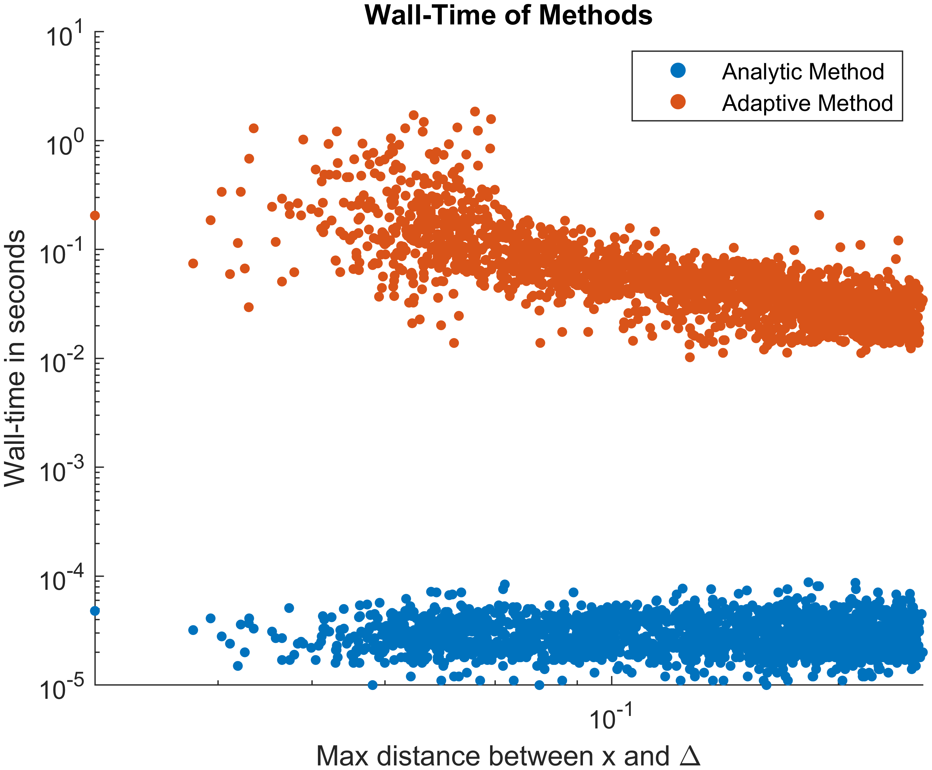
Figure 1: Wall-clock time comparison between the analytic method and adaptive method (integral2 from Matlab) on 2000 tests. The analytic method was run on Rust while the adaptive method was run in Matlab. Both languages are relatively optimized for mathematical computations, but the analytic method is more than 10 3 10^{3}
As seen in LABEL:fig:near_singular_analytic_results , the relative difference between the two methods is always below 10 − 10 10^{-10} \x \x Δ \Delta 10 − 16 10^{-16} Figure 1 10 3 10^{3}