Rethinking Benign Overfitting of Long-Tailed Data Classification in Two-layer Neural Networks

Rethinking Benign Overfitting in Two-Layer Neural Networks

Abstract

Recent theoretical studies (Kou et al., 2023; Cao et al., 2022) have revealed a sharp phase transition from benign to harmful overfitting when the noise-to-feature ratio exceeds a threshold—a situation common in long-tailed data distributions where atypical data is prevalent. However, harmful overfitting rarely happens in overparameterized neural networks. Further experimental results suggested that memorization is necessary for achieving near-optimal generalization error in long-tailed data distributions (Feldman & Zhang, 2020). We argue that this discrepancy between theoretical predictions and empirical observations arises because previous feature-noise data models overlook the heterogeneous nature of noise across different data classes. In this paper, we refine the feature-noise data model by incorporating class-dependent heterogeneous noise and re-examine the overfitting phenomenon in neural networks. Through a comprehensive analysis of the training dynamics, we establish test loss bounds for the refined model. Our findings reveal that neural networks can leverage "data noise", previously deemed harmful, to learn implicit features that improve the classification accuracy for long-tailed data. Experimental validation on both synthetic and real-world datasets supports our theoretical results.

1 Introduction

Overfitting, also known as memorization, has long been considered detrimental to model generalization performance (Hastie et al., 2009). However, with the advent of over-parameterized neural networks, models can perfectly fit the training data while still exhibiting improved generalization as model complexity increases. When and why this benign overfitting phenomenon happens have garnered significant interest within the learning theory community. Recent works, e.g., (Frei et al., 2022; Cao et al., 2022; Kou et al., 2023) showed a sharp phase transition between benign and harmful overfitting in two-layer neural networks with the feature-noise data model (Allen-Zhu & Li, 2020), which assumes data is composed of a feature vector as its mean and a random Gaussian vector as its data-specific noise. Specifically, when the magnitude of data-specific noise exceeds a threshold, the neural networks memorize the data noise, leading to harmful overfitting. Nevertheless, such harmful overfitting is rarely observed in modern over-parameterized neural networks.

Empirical evidence indicates that memorization can, in fact, enhance generalization, especially in long-tailed data distributions characterized by substantial data-specific noise (Feldman & Zhang, 2020; Hartley & Tsaftaris, 2022; Wang et al., 2024; Garg & Roy, 2023). These findings contradict current theories of the phase transition to harmful overfitting. Consequently, the following problem remains open.

How can we theoretically explain benign overfitting in overparameterized neural networks?

Inspired by the heterogeneous intra-class distributions in real datasets, we refine the feature-noise data model by incorporating class-dependent heterogeneous noise and re-examine the benign overfitting phenomenon in two-layer ReLU convolutional neural networks. In this paper, we make the following contributions:

• We establish an enhanced feature-noise model by considering class-dependent heterogeneous noise across classes. Our results with this model theoretically explain how memorization of long-tailed data boosts model performance, which cannot be predicted by existing theoretical frameworks for neural networks. Our results also show a probably counterintuitive result that a class’ classification accuracy for long-tailed data may decrease with the dataset sizes of other classes, giving an explanation to the observations in Sagawa et al. (2020).

• We derive general theoretical phase transition results between benign and harmful overfitting by analyzing the test error bound of the refined model. Our results demonstrate that although the trained neural networks can classify data through explicit features, they can additionally utilize implicit features learned through memorization of data noise to classify long-tailed data. The findings are well-supported by real datasets.

• We derive new proof techniques to tackle the randomness involved in feature learning. Unlike explicit feature learning, which exhibits stable activation states and magnitudes, data-specific noise has random activation states and magnitudes. Specifically, to tackle the random activation states, we explore the singular value distributions of neural networks to characterize the variability. Moreover, we demonstrate that the output strength of neurons randomly activated by data-specific noise is influenced by intra-class covariance matrices.

• Our analysis provides a simple model-training-free metric for evaluating data memorization, unlike previous metrics that rely on training or storing multiple models. The data with high scores on our metric correspond to visually long-tailed samples, which are memorized to benefit model generalization, aligning with Feldman & Zhang (2020); Garg & Roy (2023).

1.1 Related Work

We review the topics of empirical observations and theoretical studies of memorization.

Empirical observations of memorization. A lot of recent empirical studies have shown that memorization inevitably happens in modern over-parameterized neural networks. For instance, Feldman & Zhang (2020); Garg & Roy (2023) studied the memorization of training examples and found that neural networks tend to memorize visually atypical examples, i.e., those are rich in data-specific noise. These observations motivate us to study the impact of data-specific information on benign overfitting. In this paper, our results provide a theoretical justification for these empirical observations in neural networks.

Theoretical analyses for memorization. A body of work theoretically examined memorization within classical machine learning frameworks, demonstrating its significance for achieving near-optimal generalization performance across various contexts, including high-dimensional linear regression (Cheng et al., 2022), prediction models (Brown et al., 2021), and generalization on discrete distributions and mixture models (Feldman, 2020). This line of research failed to explain learning dynamics and generalization performance in non-convex and non-smooth neural networks.

Another line of work theoretically studied memorization in neural networks by analyzing the feature learning process during training, providing analytical frameworks that extend beyond the neural tangent kernel (NTK) regime (Jacot et al., 2018; Allen-Zhu et al., 2019; Du et al., 2018). For example, studies (e.g. (Cao et al., 2022) and (Kou et al., 2023)) explored benign overfitting in two-layer neural networks using the feature-noise model with homogeneous data noise distributions and showed a sharp phase transition between benign and harmful overfitting. However, their results all show that it is harmful to memorize data-specific information and thus fail to explain the empirical observations with long-tailed data.

1.2 Notation

We use lowercase letters, lowercase boldface letters, and uppercase boldface letters to denote scalars, vectors, and matrices, respectively. We use $[m]$ to denote the set $\{1,\cdots,m\}$. Given two sequences $\{x_{n}\}$ and $\{y_{n}\}$, we denote $x_{n}=\mathcal{O}(y_{n})$ if $|x_{n}|\leq C_{1}|y_{n}|$ for some positive constant $C_{1}$ and $x_{n}=\Omega(y_{n})$ if $|x_{n}|\geq C_{2}|y_{n}|$ for some positive constant $C_{2}$. We use $x_{n}=\Theta(y_{n})$ if $x_{n}=\mathcal{O}(y_{n})$ and $x_{n}=\Omega(y_{n})$ both hold. We use $\tilde{\mathcal{O}}(\cdot),\tilde{\Theta}(\cdot)$, and $\tilde{\Omega}(\cdot)$ to hide the logarithmic factors in these notations. Given a matrix $\mathbf{A}$, we use $\left\|\mathbf{A}\right\|_{F}$ to denote its Frobenius norm, $\left\|\mathbf{A}\right\|_{\text{op}}$ to denote its operator norm, $\mathrm{Tr}(\mathbf{A})$ to denote its trace, $\lambda_{i}(\mathbf{A})$ to denote its $i^{th}$ largest singular value, $\lambda^{+}_{\max}(\mathbf{A})$ and $\lambda^{+}_{\min}(\mathbf{A})$ to denote its maximum and minimum absolute values of non-zero singular values, and $\text{rank}(\mathbf{A})$ to denote its rank. We use the notation $(\mathbf{x},y)\sim\mathcal{D}$ to denote that the data sample $(\mathbf{x},y)$ is generated from a distribution $\mathcal{D}$.

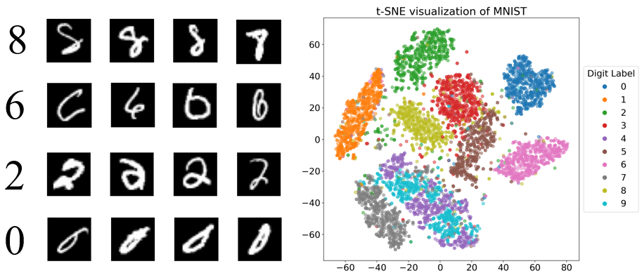
Figure 1: Left: Examples of MNIST long-tailed atypical data, which are tended to be memorized by neural networks (Feldman & Zhang, 2020). Right: t-SNE visualization of MNIST. The heterogeneous shapes imply real datasets, such as MNIST, practically show heterogeneously correlated data noise structures, providing experimental evidence for our theory.

2 Problem Setup

In this section, we introduce the problem setup including the data model, CNNs, and the training algorithm.

Given the evidence that real-world datasets have heterogeneous class-dependent data noise (as shown in Figure 1), we consider a data distribution as follows.

Data distribution. We define a data distribution $\mathcal{D}$ that each sample $(\mathbf{x},y)$ is generated as

1. Sample the label $y$ following a distribution $\mathcal{K}$, whose support is $[K]\ (K=\Theta(1))$.

2. The data $\mathbf{x}=\left(\mathbf{x}^{(1)},\mathbf{x}^{(2)}\right)$, where $\mathbf{x}^{(1)},\mathbf{x}^{(2)}\in\mathbb{R}^{d}$ contains either feature or data-specific noise patch:

• Feature patch: One patch is randomly selected as the feature patch, containing a feature vector $\mathbf{u}_{y}\in\mathbb{R}^{d}$.

• Noise patch: The remaining patch $\boldsymbol{\xi}$ is generated as $\mathbf{A}_{y}\boldsymbol{\zeta}$, where each coordinate of $\boldsymbol{\zeta}$ is i.i.d. drawn from $\mathcal{D}_{\zeta}$, a symmetric $\sigma_{p}=\Theta(1)$ sub-Gaussian distribution with variance 1, and $\mathbf{A}_{y}\in\mathbb{R}^{d\times d}$ satisfies $\mathbf{u}_{k}^{\top}\mathbf{A}_{y}=0$, for any $k\in[K]$.

Without loss of generality, we assume that the feature vectors $\mathbf{u}_{1},\cdots,\mathbf{u}_{K}$ are orthogonal and their norms are bounded, i.e., $\langle\mathbf{u}_{i},\mathbf{u}_{j}\rangle=0,\left\|\mathbf{u}_{i}\right\|_{2}=\Theta(1)$ for all $i,j\in[K]$ and $i\neq j$.

Remark 1.

The sub-Gaussian distribution of noise patches is general. In practice, pixel magnitudes in the classification tasks are bounded and thus are sub-Gaussian.

Learner model. We consider a two-layer CNN with ReLU activation as the learner model. Given an input $\mathbf{x}=\left(\mathbf{x}^{(1)},\mathbf{x}^{(2)}\right)$, the model with weights $\mathbf{W}$ outputs a $K$-length vector $[F_{1},\cdots,F_{K}]$ whose elements are

$$F_{k}\left(\mathbf{W},\mathbf{x}\right)=\mathchoice{\frac{1}{m}}{1/m}{1/m}{1/m}\sum_{r=1}^{m}\sum_{j=1}^{2}\sigma\left(\left\langle\mathbf{w}_{k,r},\mathbf{x}^{(j)}\right\rangle\right),$$ (1)

where $\sigma(z)=\max\{0,z\}$ denotes the ReLU activation function, $\mathbf{w}_{k,r}$ denotes the weight vector for the $r^{th}$ neuron (totally $m$ neurons) associated with $F_{k}(\mathbf{W},\mathbf{x})$.

Training objective. Given a training dataset with $n$ samples $\mathcal{S}=\{(\mathbf{x}_{i},y_{i})\}_{i=1}^{n}$ drawn from the distribution $\mathcal{D}$, we train the neural network by minimizing the empirical risk with the cross-entropy loss, i.e.,

$$\mathcal{L}_{\mathcal{S}}\left(\mathbf{W}\right)=\mathchoice{\frac{1}{n}}{1/n}{1/n}{1/n}\sum_{i=1}^{n}\mathcal{L}(\mathbf{W},\mathbf{x}_{i},y_{i}),$$ (2)

where $\mathcal{L}(\mathbf{W},\mathbf{x},y)=-\log(\text{logit}_{y}(\mathbf{W},\mathbf{x}))$, and $\text{logit}(\cdot)$ represents the output probability of the neural network:

$$\text{logit}_{y}(\mathbf{W},\mathbf{x})=\mathchoice{\frac{\exp(F_{y}(\mathbf{W},\mathbf{x}))}{\sum_{k=1}^{K}\exp(F_{k}(\mathbf{W},\mathbf{x}))}}{\exp(F_{y}(\mathbf{W},\mathbf{x}))/\sum_{k=1}^{K}\exp(F_{k}(\mathbf{W},\mathbf{x}))}{\exp(F_{y}(\mathbf{W},\mathbf{x}))/\sum_{k=1}^{K}\exp(F_{k}(\mathbf{W},\mathbf{x}))}{\exp(F_{y}(\mathbf{W},\mathbf{x}))/\sum_{k=1}^{K}\exp(F_{k}(\mathbf{W},\mathbf{x}))}.$$ (3)

Initialization. The initial weights of the neural network’s parameters are generated i.i.d. from Gaussian distribution, i.e., $\mathbf{w}^{(0)}_{j,r}\sim\mathcal{N}(\mathbf{0},\sigma_{0}^{2}\mathbf{I})$, for all $j\in[K],r\in[m]$.

Training algorithm. We train the neural network by gradient descent (GD) with a learning rate $\eta$, i.e.,

$$\mathbf{W}^{(t+1)}=\mathbf{W}^{(t)}-\mathchoice{\frac{\eta}{n}}{\eta/n}{\eta/n}{\eta/n}\sum_{(\mathbf{x},y)\in\mathcal{S}}\nabla\mathcal{L}(\mathbf{W}^{(t)},\mathbf{x},y).$$ (4)

3 Main Results

In this section, we present our main theoretical results. We start by introducing some conditions for our theory.

Our analyses rely on the following conditions on noise patch distributions, training dataset size $n$, network width $m$, dimension $d$, learning rate $\eta$, and initialization $\sigma_{0}$.

Condition 1.

Suppose there exists a sufficiently large constant $C$. For certain probability parameter $\delta\in(0,1)$, the following conditions hold:

1. To ensure that the neurons can learn the data patterns, the noise patch distributions satisfy, for any $i,j\in[K]$,

   $$\begin{cases}\mathrm{Tr}(\mathbf{A}_{i}^{\top}\mathbf{A}_{i})\geq Cn\left\|\mathbf{A}_{i}^{\top}\mathbf{A}_{j}\right\|_{F}\log(\mathchoice{\frac{n^{2}}{\delta}}{n^{2}/\delta}{n^{2}/\delta}{n^{2}/\delta}),\\ \mathchoice{\frac{\left\|\mathbf{A}_{i}^{\top}\mathbf{A}_{j}\right\|_{F}}{\left\|\mathbf{A}_{i}^{\top}\mathbf{A}_{j}\right\|_{\textnormal{op}}}}{\left\|\mathbf{A}_{i}^{\top}\mathbf{A}_{j}\right\|_{F}/\left\|\mathbf{A}_{i}^{\top}\mathbf{A}_{j}\right\|_{\textnormal{op}}}{\left\|\mathbf{A}_{i}^{\top}\mathbf{A}_{j}\right\|_{F}/\left\|\mathbf{A}_{i}^{\top}\mathbf{A}_{j}\right\|_{\textnormal{op}}}{\left\|\mathbf{A}_{i}^{\top}\mathbf{A}_{j}\right\|_{F}/\left\|\mathbf{A}_{i}^{\top}\mathbf{A}_{j}\right\|_{\textnormal{op}}}\geq C\sqrt{\log(\mathchoice{\frac{K}{\delta}}{K/\delta}{K/\delta}{K/\delta})},\\ \left\|\mathbf{A}_{i}^{\top}\mathbf{A}_{j}\right\|_{F}\geq C^{-1}\max_{k\neq j}\{\left\|\mathbf{A}_{i}^{\top}\mathbf{A}_{k}\right\|_{F}\}.\end{cases}$$

   Moreover, there exists a threshold $c^{\prime}>0$ such that $\mathbb{P}[\zeta>c^{\prime}]\geq 0.4$.

2. To ensure that the learning problem is in a sufficiently over-parameterized setting, the training dataset size $n$, network width $m$, and dimension $d$ satisfy

   $$\begin{cases}m\geq C\log(n/\delta)\max_{i}\{\mathchoice{\frac{(\lambda_{\max}^{+}(\mathbf{A}_{i}))^{2}}{(\lambda_{\min}^{+}(\mathbf{A}_{i}))^{2}}}{(\lambda_{\max}^{+}(\mathbf{A}_{i}))^{2}/(\lambda_{\min}^{+}(\mathbf{A}_{i}))^{2}}{(\lambda_{\max}^{+}(\mathbf{A}_{i}))^{2}/(\lambda_{\min}^{+}(\mathbf{A}_{i}))^{2}}{(\lambda_{\max}^{+}(\mathbf{A}_{i}))^{2}/(\lambda_{\min}^{+}(\mathbf{A}_{i}))^{2}}\},\\ n\geq C\log(m/\delta),m\geq\Omega\left(\mathchoice{\frac{\log(\mathchoice{\frac{n}{\delta}}{n/\delta}{n/\delta}{n/\delta})\log(T)^{2}}{n\sigma_{0}^{2}}}{\log(\mathchoice{\frac{n}{\delta}}{n/\delta}{n/\delta}{n/\delta})\log(T)^{2}/n\sigma_{0}^{2}}{\log(\mathchoice{\frac{n}{\delta}}{n/\delta}{n/\delta}{n/\delta})\log(T)^{2}/n\sigma_{0}^{2}}{\log(\mathchoice{\frac{n}{\delta}}{n/\delta}{n/\delta}{n/\delta})\log(T)^{2}/n\sigma_{0}^{2}}\right),\\ \min\{m,d,\text{rank}(\mathbf{A}_{j})\}-0.9m\geq Cn,\\ d\geq C\log(\mathchoice{\frac{mn}{\delta}}{mn/\delta}{mn/\delta}{mn/\delta}).\end{cases}$$

3. To ensure that gradient descent can minimize the training loss, the learning rate $\eta$ and initialization $\sigma_{0}$ satisfy, for any $j\in[K]$,

   $$\begin{cases}\!\eta\!\leq\!\!\left(\!\!C\!\left(\!\max_{k\in[K]}\!\left(\!\left\|\mathbf{u}_{k}\right\|_{2}\!+\!\!\sqrt{\!1.5\mathrm{Tr}\left(\mathbf{A}_{k}^{\top}\mathbf{A}_{k}\right)}\!\right)\!\right)^{2}\!\right)^{-1},\\ \eta\leq\mathchoice{\frac{mn\log(T)}{\mathrm{Tr}(\mathbf{A}_{j}^{\top}\mathbf{A}_{j})}}{mn\log(T)/\mathrm{Tr}(\mathbf{A}_{j}^{\top}\mathbf{A}_{j})}{mn\log(T)/\mathrm{Tr}(\mathbf{A}_{j}^{\top}\mathbf{A}_{j})}{mn\log(T)/\mathrm{Tr}(\mathbf{A}_{j}^{\top}\mathbf{A}_{j})},\\ \sigma_{0}\leq\!C^{-1}n^{-1}\phi\cdot$ $\!\\ \!\!\left(\!\max_{k\in[K]}\!\{\!\sqrt{\log(\!Km/\!\delta)}\!\!\left\|\mathbf{u}_{k}\right\|_{2}\!,\!\!\log(\!Km/\!\delta)\!\left\|\mathbf{A}_{k}\right\|\!\!_{F}\!\}\!\!\right)^{-1}\!\!,\end{cases}$$

   where $\phi:=\min_{k_{1},k_{2}\in[K]}\{\left\|\mathbf{A}_{k_{1}}^{\top}\mathbf{A}_{k_{2}}\right\|_{F},\left\|\mathbf{u}_{k_{1}}\right\|_{2}^{2}\}$.

Based on Condition 1, we study the model convergence and generalization performance by bounding the training loss and the zero-one test loss (accuracy) of the trained model $\mathbf{W}^{(T)}$ on distribution $\mathcal{D}_{k}$ whose probability density function is $\mathbb{P}_{\mathcal{D}_{k}}[(\mathbf{x},y)]=\mathbb{P}_{\mathcal{D}}[(\mathbf{x},y)|y=k]$, i.e., for all $k\in[K]$,

$$\mathcal{L}^{0-1}_{\mathcal{D}_{k}}(\mathbf{W}^{(T)})$$

$$= \mathbb{P}_{(\mathbf{x},y)\sim\mathcal{D}_{k}}\left[F_{y}(\mathbf{W}^{(T)},\mathbf{x})\neq\max_{j\in[K]}\{F_{j}(\mathbf{W}^{(T)},\mathbf{x})\}\right].$$

Before presenting the main theorem, we define the set of long-tailed data with respect to the trained model $\mathbf{W}^{(T)}$.

Definition 1 ($L$-Long-tailed data set).

The $L$-long-tailed data distribution $\mathcal{T}_{j}$ for each $j\in[K]$ with model $\mathbf{W}^{(T)}$ is defined as

$$\mathbb{P}_{\mathcal{T}_{j}}[(\mathbf{x},y)]=$$

$$\mathbb{P}_{\mathcal{D}_{j}}\left[(\mathbf{x},y)|\langle\sum_{r\in\mathcal{R}(\boldsymbol{\xi})}\mathbf{w}^{(T)}_{y,r},\boldsymbol{\xi}\rangle\!=\!\Omega(L\|\mathbf{A}_{y}^{\top}\!\sum_{r\in\mathcal{R}(\boldsymbol{\xi})}\mathbf{w}^{(T)}_{y,r}\|_{2})\right],$$

where $\mathcal{R}(\boldsymbol{\xi})=\{r\in[m]:\langle\mathbf{w}^{(T)}_{y,r},\boldsymbol{\xi}\rangle>0\}$.

Definition 1 identifies data whose equivalent noise $\zeta^{\prime}$ exceeds a threshold. Specifically, for data $(\mathbf{x},y)\sim\mathcal{D}$, the inner product term $\langle\sum_{r\in\mathcal{R}(\boldsymbol{\xi})}\mathbf{w}^{(T)}_{y,r},\boldsymbol{\xi}\rangle$ satisfies $\langle\sum_{r\in\mathcal{R}(\boldsymbol{\xi})}\mathbf{w}^{(T)}_{y,r},\boldsymbol{\xi}\rangle=\Theta\left(\left\|\mathbf{A}_{y}^{\top}\sum_{r\in\mathcal{R}(\boldsymbol{\xi})}\mathbf{w}^{(T)}_{y,r}\right\|_{2}\zeta^{\prime}\right)$, where $\zeta^{\prime}$ is an equivalent random sub-Gaussian variable with variance 1.

Remark 2.

Model-dependent long-tailed definitions are common. Feldman & Zhang (2020) defined the long-tailed data using an influence score that measures the training loss difference on datasets with and without a data sample. Garg & Roy (2023) defined the long-tailedness of data using a curvature metric that approximates a loss Hessian matrix-related quantity of trained models averaged over all training epochs.

We denote $\mathcal{S}_{j}$ as the set containing training data with label $j$ in $\mathcal{S}$. We present our main result in the following theorem.

Theorem 1.

For any $\epsilon>0$ and $k\in[K]$, under Condition 1, there exists $T=\tilde{\mathcal{O}}(\eta^{-1}\epsilon^{-1}\!\max\{n\max_{j\in[K]}\{\mathrm{Tr}(\mathbf{A}_{j}^{\top}\mathbf{A}_{j})\},\sqrt{md}\sigma_{0},\!\sqrt{mK}\})$, with probability at least $1-\delta$, the following holds:

1. The training loss satisfies $\mathcal{L}_{\mathcal{S}}(\mathbf{W}^{(T)})\leq\epsilon$.

2. Benign overfitting:

   1. (For all data) When the signal-to-noise ratio is large, i.e., $|\mathcal{S}_{k}|^{2}\left\|\mathbf{u}_{k}\right\|_{2}^{4}\geq C_{1}\cdot\max_{j\neq k}\{|\mathcal{S}_{j}|\left\|\mathbf{A}_{k}^{\top}\mathbf{A}_{j}\right\|_{F}^{2}\}$, the zero-one test loss satisfies

      $$\mathcal{L}^{0-1}_{\mathcal{D}_{k}}(\mathbf{W}^{(T)})\!\leq\!\sum_{j\neq k}\exp\!\left(\!-c_{1}\cdot\underbrace{\mathchoice{\frac{|\mathcal{S}_{k}|^{2}\left\|\mathbf{u}_{k}\right\|_{2}^{4}}{|\mathcal{S}_{j}|\left\|\mathbf{A}_{k}^{\top}\mathbf{A}_{j}\right\|_{F}^{2}}}{|\mathcal{S}_{k}|^{2}\left\|\mathbf{u}_{k}\right\|_{2}^{4}/|\mathcal{S}_{j}|\left\|\mathbf{A}_{k}^{\top}\mathbf{A}_{j}\right\|_{F}^{2}}{|\mathcal{S}_{k}|^{2}\left\|\mathbf{u}_{k}\right\|_{2}^{4}/|\mathcal{S}_{j}|\left\|\mathbf{A}_{k}^{\top}\mathbf{A}_{j}\right\|_{F}^{2}}{|\mathcal{S}_{k}|^{2}\left\|\mathbf{u}_{k}\right\|_{2}^{4}/|\mathcal{S}_{j}|\left\|\mathbf{A}_{k}^{\top}\mathbf{A}_{j}\right\|_{F}^{2}}}_{\text{signal-to-noise ratio}}\right)\!.$$

   2. (Only for long-tailed data) When the noise correlation ratio is large, i.e.,$|\mathcal{S}_{k}|\left\|\mathbf{A}_{k}^{\top}\mathbf{A}_{k}\right\|_{F}^{2}\geq C_{2}\cdot\max_{j\neq k}\{|\mathcal{S}_{j}|\left\|\mathbf{A}_{k}^{\top}\mathbf{A}_{j}\right\|_{F}^{2}\}$, the zero-one test loss satisfies

      $$\mathcal{L}^{0-1}_{\mathcal{T}_{k}}(\mathbf{W}^{(T)})$$

      $$\leq \sum_{j\neq k}\exp\left(-c_{2}L^{2}\cdot\underbrace{\mathchoice{\frac{|\mathcal{S}_{k}|\left\|\mathbf{A}_{k}^{\top}\mathbf{A}_{k}\right\|_{F}^{2}}{|\mathcal{S}_{j}|\left\|\mathbf{A}_{k}^{\top}\mathbf{A}_{j}\right\|_{F}^{2}}}{|\mathcal{S}_{k}|\left\|\mathbf{A}_{k}^{\top}\mathbf{A}_{k}\right\|_{F}^{2}/|\mathcal{S}_{j}|\left\|\mathbf{A}_{k}^{\top}\mathbf{A}_{j}\right\|_{F}^{2}}{|\mathcal{S}_{k}|\left\|\mathbf{A}_{k}^{\top}\mathbf{A}_{k}\right\|_{F}^{2}/|\mathcal{S}_{j}|\left\|\mathbf{A}_{k}^{\top}\mathbf{A}_{j}\right\|_{F}^{2}}{|\mathcal{S}_{k}|\left\|\mathbf{A}_{k}^{\top}\mathbf{A}_{k}\right\|_{F}^{2}/|\mathcal{S}_{j}|\left\|\mathbf{A}_{k}^{\top}\mathbf{A}_{j}\right\|_{F}^{2}}}_{\text{noise correlation ratio }\Gamma_{k,j}}\right).$$

3. Harmful overfitting: When the signal-to-noise ratio and noise correlation ratio are small, i.e., $|\mathcal{S}_{k}|^{2}\left\|\mathbf{u}_{k}\right\|_{2}^{4}\leq C_{3}\cdot\max_{j\neq k}\{|\mathcal{S}_{j}|\left\|\mathbf{A}_{k}^{\top}\mathbf{A}_{j}\right\|_{F}^{2}\}$ and $|\mathcal{S}_{k}|\left\|\mathbf{A}_{k}^{\top}\mathbf{A}_{k}\right\|_{F}^{2}\leq C_{3}\cdot\max_{j\neq k}\{|\mathcal{S}_{j}|\left\|\mathbf{A}_{k}^{\top}\mathbf{A}_{j}\right\|_{F}^{2}\}$, the zero-one test loss satisfies $\mathcal{L}^{0-1}_{\mathcal{D}_{k}}(\mathbf{W}^{(T)})\geq c_{3}$.

Here $C_{1},C_{2},C_{3},c_{1},c_{2},c_{3}$ are some absolute constants.

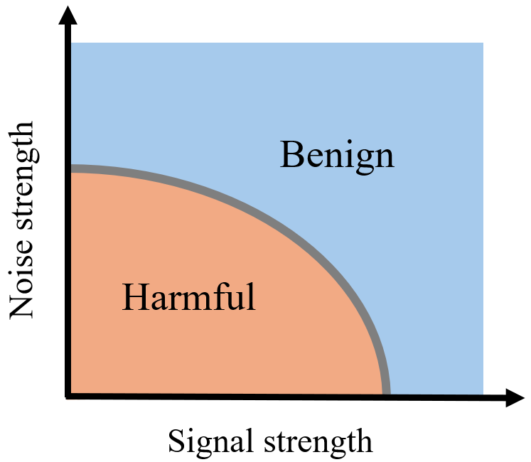
Figure 2: Illustration of the generalized phased transition between benign and harmful overfitting (memorization). The blue region represents a benign overfitting regime where the test loss is small. The orange region represents a harmful overfitting regime where the test loss is at a constant order. The gray band region is the setting where the test loss is not well characterized.

Remark 3.

Theorem 1 shows that after $T$ iterations, CNNs converge to training loss $\epsilon$ (Statement 1). When the signal-to-noise ratio is high, the trained CNNs can achieve optimal test loss by effectively detecting explicit features $\mathbf{u}_{k}$ (Statement 2(a)). Furthermore, CNNs also classify long-tailed data by seeking to detect data-specific features so that the performance benefits from high noise correlation ratios (Statement 2(b)). Conversely, when both noise correlation ratios and signal-to-noise ratios are small, the trained CNNs incur test loss at least a constant (Statement 3). Notably, longer-tailed data (with a larger $L$) benefits more from the data-specific noise.

Remark 4.

Theorem 1 characterizes a sharp phase transition between benign and harmful overfitting (memorization), visualized in Figure 2. Statement 2(a) in Theorem 1 extends the previous benign overfitting results, which characterize the horizontal dimension in Figure. 2. Statement 2(b) in Theorem 1 at the first time characterizes the vertical dimension in Figure. 2, showing that the model can also leverage data-specific noise to achieve benign overfitting.

Remark 5.

By choosing $\mathbf{A}_{j}\mathbf{A}_{j}^{\top}=\mathbf{I}-\sum_{k=1}^{K}\mathbf{u}_{k}\mathbf{u}_{k}^{\top}/\left\|\mathbf{u}_{k}\right\|_{2}^{2}$ for all $j\in[K]$, our Statement 2(a) recovers the same convergence orders in the standard benign overfitting results (Kou et al., 2023). However, our results are more general as our results cover the whole class of sub-Gaussian data noise, $K>2$ number of classes, and data imbalance, which is common in modern image classification tasks.

The results of Theorem 1 theoretically explain the following two empirical observations in neural networks for the first time.

Long-tailed (atypical) data is important for generalization. In Statement 2(b) of Theorem 1, we show that the classification accuracy of long-tailed data increases with the noise correlation ratio. This result implies that incorporating more long-tailed data into the training dataset enhances test accuracy, providing a theoretical explanation for the empirical observation in Feldman & Zhang (2020) that including long-tailed data in the training dataset is necessary for neural networks to achieve near-optimal generalization performance.

Increasing majority hurts minority. Statement 2(b) of Theorem 1 implies that as the dataset size of class $j$, $|\mathcal{S}_{j}|$ increases, the upper bound on test loss of other classes $k\neq j$ increases. This leads to a possibly surprising result: the classification accuracy for long-tailed data of a specific class may decline when the sizes of other classes increase. The reason is that during training, the memorization of majority data-specific noise (classes with more data) dominates the memorization of minority data-specific noise. Our result theoretically explains a counter-intuitive observation in neural networks that subsampling the majority group empirically achieves low minority error (Sagawa et al., 2020).

4 Proof Overview

In this section, we present a proof sketch of Statement 1 and Statement 2(b) in Theorem 1 (Statement 2(a) uses a similar but simpler proof). Due to the space limit, we defer the complete proofs to Appendices A, B, and C.

4.1 Proof Sketch of Statement 1 in Theorem 1

We analyze the training loss in two stages. In training Stage 1, the training loss of each example decreases exponentially and stays at a constant order $\Theta(1)$. In Stage 2, the model converges to an arbitrarily small constant.

Stage 1.

By the nature of cross-entropy, the training loss decreases exponentially, characterized by the following lemma.

Lemma 1.

Under Condition 1, there exists an iteration number $T_{0}=\tilde{\mathcal{O}}(\mathchoice{\frac{mn}{\eta}}{mn/\eta}{mn/\eta}{mn/\eta})$, so that for any $(\mathbf{x},y)\in\mathcal{S}$ and $t\leq T_{0}$, the following holds:

$$\mathcal{L}(\mathbf{W}^{(t+1)},\mathbf{x},y)$$ (5)

$$\leq \left(1-\Theta\left(\mathchoice{\frac{\eta}{mn}}{\eta/mn}{\eta/mn}{\eta/mn}|\mathcal{S}_{y}|\left\|\mathbf{u}_{y}\right\|_{2}^{2}\right)\right)\mathcal{L}(\mathbf{W}^{(t)},\mathbf{x},y).$$

Stage 2.

We show that the training loss converges to an arbitrarily small constant $\epsilon$ with a rate of $\mathcal{O}(\mathchoice{\frac{1}{T}}{1/T}{1/T}{1/T})$.

Lemma 2.

Let $\mathbf{W}^{*}$ be the network parameters with each neuron $\mathbf{w}_{j,r}^{*}=2.5\log\left(\mathchoice{\frac{4(K-1)}{\epsilon}}{4(K-1)/\epsilon}{4(K-1)/\epsilon}{4(K-1)/\epsilon}\right)\mathchoice{\frac{\mathbf{u}_{j}}{\left\|\mathbf{u}_{j}\right\|_{2}^{2}}}{\mathbf{u}_{j}/\left\|\mathbf{u}_{j}\right\|_{2}^{2}}{\mathbf{u}_{j}/\left\|\mathbf{u}_{j}\right\|_{2}^{2}}{\mathbf{u}_{j}/\left\|\mathbf{u}_{j}\right\|_{2}^{2}}$. Under Condition 1, for any $t\in[T_{0},T]$ and $(\mathbf{x},y)\in\mathcal{S}$, the following result holds:

$$\mathchoice{\frac{1}{t-T_{0}+1}}{1/t-T_{0}+1}{1/t-T_{0}+1}{1/t-T_{0}+1}\sum_{s=T_{0}}^{t}\mathcal{L}_{S}(\mathbf{W}^{(t)})\leq \mathchoice{\frac{\left\|\mathbf{W}^{(T_{0})}-\mathbf{W}^{*}\right\|_{F}^{2}}{\eta(t-T_{0}+1)}}{\left\|\mathbf{W}^{(T_{0})}-\mathbf{W}^{*}\right\|_{F}^{2}/\eta(t-T_{0}+1)}{\left\|\mathbf{W}^{(T_{0})}-\mathbf{W}^{*}\right\|_{F}^{2}/\eta(t-T_{0}+1)}{\left\|\mathbf{W}^{(T_{0})}-\mathbf{W}^{*}\right\|_{F}^{2}/\eta(t-T_{0}+1)}+\mathchoice{\frac{\epsilon}{2}}{\epsilon/2}{\epsilon/2}{\epsilon/2}.$$

After $T=\tilde{\mathcal{O}}(\eta^{-1}\epsilon^{-1}\!\max\{n\max_{j\in[K]}\{\mathrm{Tr}(\mathbf{A}_{j}^{\top}\mathbf{A}_{j})\},$ $\sqrt{md}\sigma_{0},\!\sqrt{mK}\})$ iterations, the training loss converges to $\epsilon$. Our analysis extends that of Kou et al. (2023) by providing the convergence rate for Stage 1 and a comprehensive convergence analysis for $K$-class classification problems using cross-entropy loss.

4.2 Proof Sketch of Statement 2(b) in Theorem 1

By the definition of zero-one test loss, for any long-tailed data $(\mathbf{x},y)\in\mathcal{T}_{i},i\in[K]$, its test loss satisfies:

$$\mathcal{L}^{0-1}_{\mathcal{T}_{i}}(\mathbf{W}^{(T)})\leq\sum_{j\neq i}$$

$$\!\mathbb{P}_{(\mathbf{x},y)\sim\mathcal{T}_{i}}\!\!\!\left[\sum_{r=1}^{m}\!\sigma(\!\langle\mathbf{w}_{y,r}^{(T)}\!,\boldsymbol{\xi}\rangle\!)\!\leq\!\!\sum_{r=1}^{m}\!\sigma(\!\langle\mathbf{w}_{j,r}^{(T)}\!,\!\mathbf{u}_{y}\rangle\!)\!+\!\sigma(\!\langle\mathbf{w}_{j,r}^{(T)}\!,\boldsymbol{\xi}\rangle\!)\!\right]\!\!.$$

Roughly speaking, since the neurons for a class do not learn explicit features for other classes, i.e., $\sum_{r=1}^{m}\!\sigma(\langle\mathbf{w}_{j,r}^{(T)},\mathbf{u}_{y}\rangle)$ is small, the key to quantifying the test loss is to compare the correlation coefficients $\sum_{r=1}^{m}\sigma(\langle\mathbf{w}_{y,r}^{(T)},\boldsymbol{\xi}\rangle)$ and $\sum_{r=1}^{m}\sigma(\langle\mathbf{w}_{j,r}^{(T)},\boldsymbol{\xi}\rangle)$. Firstly, we need to quantify the number of neurons that can be activated by the random data-specific noise $\boldsymbol{\xi}$. We leverage the properties of the rank and singular values of the neurons corresponding to each class $j\in[K]$, i.e., $\mathbf{W}_{j}^{(T)}=[\mathbf{w}_{j,1}^{(T)},\cdots,\mathbf{w}_{j,m}^{(T)}]^{\top}$, in the following lemma.

Lemma 3.

Under condition 1, the matrix $\mathbf{W}_{j}^{(T)}$ for all $j\in[K]$ satisfies

$$\textnormal{rank}(\mathbf{W}_{j}^{(T)}\mathbf{A}_{j})\geq 0.9m,\ \lambda_{1}(\mathbf{W}_{j}^{(T)}\mathbf{A}_{j})\leq\mathcal{O}(\sqrt{m}\log(T)),$$

$$\lambda_{\min\{m,d,\textnormal{rank}(\mathbf{A}_{j})\}-n}(\mathbf{W}_{j}^{(T)}\mathbf{A}_{j})\geq 0.1\sqrt{m}\sigma_{0}.$$

With Lemma 3, we can prove that the probability that $\langle\mathbf{w}_{y,r}^{(T)},\boldsymbol{\xi}\rangle$ remains in an orthant decreases exponentially with the number of neurons $m$. Consequently, we derive the following lemma for the number of activated neurons.

Lemma 4.

Under condition 1, for any $j\in[K]$ and any $(\mathbf{x},y)\sim\mathcal{D}_{j}$, with probability at least $1-\exp(-\Omega(m))$, the trained model $\mathbf{W}^{(T)}$ satisfies

$$\sum_{r=1}^{m}\mathbb{I}\left(\langle\mathbf{w}_{j,r}^{(T)},\boldsymbol{\xi}\rangle\right)\geq 0.1m.$$ (6)

Lemma 4 indicates that, with high probability, at least a non-negligible amount of neurons are able to detect the data-specific noise in the test data. Next, we quantify the activation magnitude of the correlation coefficients $\sum_{r=1}^{m}\sigma(\langle\mathbf{w}_{y,r}^{(T)},\boldsymbol{\xi}\rangle)$ and $\sum_{r=1}^{m}\sigma(\langle\mathbf{w}_{j,r}^{(T)},\boldsymbol{\xi}\rangle)$. In the following lemma, we prove that the neurons for class $j\in[K]$ mainly learn the data noise from class $j$.

Lemma 5.

Under Condition 1, for any $j\in[K],l\in[K]\backslash\{j\},(\mathbf{x}_{q},y_{q})\in\mathcal{S}_{j},(\mathbf{x}_{a},y_{a})\in\mathcal{S}_{l}$, existing a sufficiently large constant $C^{\prime}>0$, we have

$$\sum_{r=1}^{m}\sigma(\langle\mathbf{w}_{j,r}^{(T)},\boldsymbol{\xi}_{q}\rangle)\geq C^{\prime}\sum_{r=1}^{m}\sigma(\langle\mathbf{w}_{j,r}^{(T)},\boldsymbol{\xi}_{a}\rangle).$$ (7)

As a result, the order of activation magnitudes is controlled by the intra-class correlations and inter-class correlations, quantified by $\|\mathbf{A}_{y}^{\top}\mathbf{A}_{y}\|_{F}$ and $\|\mathbf{A}_{y}^{\top}\mathbf{A}_{j}\|_{F}$.

Lemma 6.

Under Condition 1, for any $(\mathbf{x},y)\sim\mathcal{T}_{i}$ and $i\in[K],j\in[K]\backslash\{y\}$, the following holds:

$$\sum_{r=1}^{m}\sigma\left(\langle\mathbf{w}_{y,r}^{(T)},\boldsymbol{\xi}\rangle\right)=\Theta\left(\mathchoice{\frac{\eta m}{n}}{\eta m/n}{\eta m/n}{\eta m/n}\left\|\mathbf{A}_{y}^{\top}\mathbf{A}_{y}\right\|_{F}Lb(\mathcal{S}_{y})\right),$$

$$\sum_{r=1}^{m}\sigma\left(\langle\mathbf{w}^{(T)}_{j,r},\boldsymbol{\xi}\rangle\right)=\mathcal{O}\left(\mathchoice{\frac{\eta m}{n}}{\eta m/n}{\eta m/n}{\eta m/n}\left\|\mathbf{A}_{y}^{\top}\mathbf{A}_{j}\right\|_{F}b(\mathcal{S}_{j})|\zeta_{1}|\right),$$

where $b(\cdot)$ is a function defined as

$$b(\mathcal{A})=\sqrt{\sum_{(\mathbf{x},y)\in\mathcal{A}}\left(\sum_{t^{\prime}=0}^{T-1}(1-\textnormal{logit}_{y}(\mathbf{W}^{(t^{\prime})},\mathbf{x}))\right)^{2}},$$ (8)

and $\zeta_{1}$ is a sub-Gaussian variable with variance 1.

Finally, to compare $b(\mathcal{S}_{y})$ and $b(\mathcal{S}_{j})$, we prove that the loss gradient coefficients are balanced.

Lemma 7.

For all $t\in[T]$ and for any $i,j\in[n]$, there exists a positive constant $\kappa$ such that

$$\mathchoice{\frac{1-\textnormal{logit}_{y_{i}}(\mathbf{W}^{(t)},\mathbf{x}_{i})}{1-\textnormal{logit}_{y_{j}}(\mathbf{W}^{(t)},\mathbf{x}_{j})}}{1-\textnormal{logit}_{y_{i}}(\mathbf{W}^{(t)},\mathbf{x}_{i})/1-\textnormal{logit}_{y_{j}}(\mathbf{W}^{(t)},\mathbf{x}_{j})}{1-\textnormal{logit}_{y_{i}}(\mathbf{W}^{(t)},\mathbf{x}_{i})/1-\textnormal{logit}_{y_{j}}(\mathbf{W}^{(t)},\mathbf{x}_{j})}{1-\textnormal{logit}_{y_{i}}(\mathbf{W}^{(t)},\mathbf{x}_{i})/1-\textnormal{logit}_{y_{j}}(\mathbf{W}^{(t)},\mathbf{x}_{j})}\leq\kappa.$$ (9)

Leveraging Hoeffding’s inequality, Lemma 6, and 7, we derive Statement 2(b) in Theorem 1.

5 Experiments

In this section, we first validate our theory in Theorem 1 by constructing datasets and models following our problem setup in Section 2. We further verify our conclusions with real-world datasets MNIST (LeCun et al., 1998) and CIFAR-10 (Krizhevsky et al., 2009).

5.1 Synthetic Datasets

Synthetic data generation. We generate a synthetic dataset following the data distribution outlined in Section 2. The dataset comprises a total of $K=5$ classes with a dimensionality of $d=1000$. We set the feature patches for each $k\in[K]$ as $\mathbf{u}_{k}=\mathbf{U}\cdot\left\|\mathbf{u}_{k}\right\|_{2}\cdot\mathbf{z}_{k}$, where $\mathbf{z}_{k}$ keeps the $k^{th}$ entry to be one and other entries zeros, and $\mathbf{U}$ is a randomly generated unitary matrix. Without loss of generality, we consider $\mathbf{A}_{k}$ to be matrices with all but one non-zero eigenvalue fixed as 0.5. Then, we tune the not-fixed non-zero eigenvalue to change the noise correlation ratio accordingly.

Setup. We train a two-layer neural network as defined in Section 2 with $m=100$ neurons. We use the default initialization method in PyTorch to initialize the neurons’ parameters. We train the neural networks using GD with a learning rate $\eta=0.05$ over $20$ epochs. To explore the effects of feature strength $\left\|\mathbf{u}_{i}\right\|_{2}$, noise correlation ratio $\Gamma_{i,j}$, and dataset size $|\mathcal{S}_{i}|$, we simply fix $\left\|\mathbf{u}_{i}\right\|_{2}=\left\|\mathbf{u}\right\|_{2}$, $\Gamma_{i,j}=\Gamma$, and $|\mathcal{S}_{i}|=s$, where $\left\|\mathbf{u}\right\|_{2}$, $\Gamma$, and $s$ are tunable parameters for all class $i,j\in[K]\ (j\neq i)$.

Effects of noise correlation and feature strength. We simulate with feature strength $\left\|\mathbf{u}\right\|_{2}$ ranging from $0.001$ to $3.8$ and noise correlation ratio $\Gamma$ ranging from $1$ to $1400$. We fix the dataset size of each class as $|\mathcal{S}_{i}|=100$, for all $i\in[K]$. The resulting heatmap of test accuracy in relation to data feature size and noise correlation is presented in Figure 3. As illustrated, the test loss decreases not only with increasing feature strength, but also with higher noise correlation ratios. Notably, with high noise correlation ratios, we can achieve near-optimal test accuracy even when feature strength approaches nearly zero.

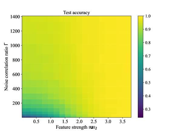
(a) Test accuracy heatmap under Gaussian data noise. Each entry of $\zeta$ follows $\mathcal{N}(0,1)$.

(b) Test accuracy heatmap under uniform data noise. Each entry of $\zeta$ follows $\mathcal{U}(-\sqrt{3},\sqrt{3})$.

Figure 3: Impacts of feature strength and noise correlation ratio on test accuracy.

Effect of dataset size. We verify the impact of the dataset sizes in the two types of benign overfitting in Statement (a) and (b) of Theorem 1. We fix the noise correlation ratio as $\Gamma=1.2$ with $\zeta$ following Gaussian distribution and vary the feature size ranging from $0.01$ to 4 and dataset size ranging from $10$ to $200$ to explore the effect of dataset size versus feature strength on test accuracy (Figure 4(a)). We fix the feature strength as $\left\|\mathbf{u}\right\|_{2}=1e-6$ and tune noise correlation ratio $\Gamma$ (with $\zeta$ following Gaussian distribution) ranging from 1 to 800 and dataset size ranging from $10$ to $200$ to explore the effect of dataset size versus noise correlation ratio (Figure 4(b)). These results verify our theory. Specifically, for classification utilizing explicit features (Figure. 4(a)), the test accuracy increases with increasing dataset size, matching our Statement 2(a) in Theorem 1. In contrast, for classification utilizing implicit covariance features (Figure 4(b)), the test accuracy remains in a constant order with the dataset size, matching Statement 2(b) in Theorem 1.

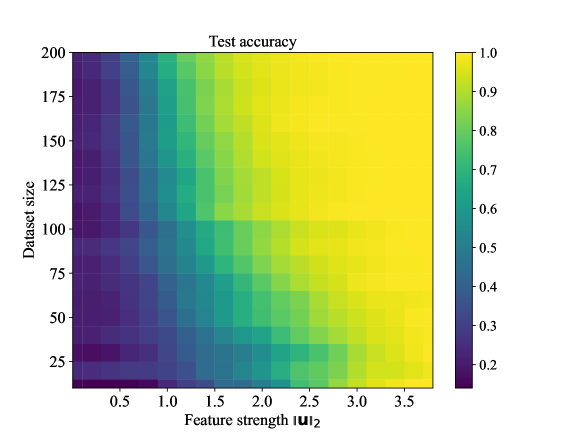
(a) Test accuracy heatmap with feature strength and dataset size. Each entry of $\zeta$ follows $\mathcal{N}(0,1)$.

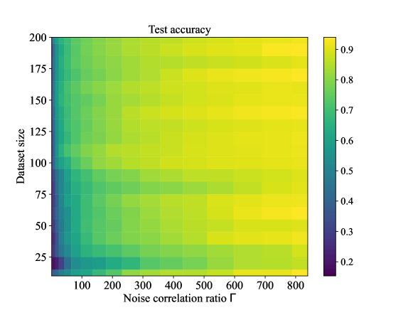
(b) Test accuracy heatmap with noise correlation ratio and dataset size. Each entry of $\zeta$ follows $\mathcal{N}(0,1)$.

Figure 4: Impacts of data size on test accuracy.

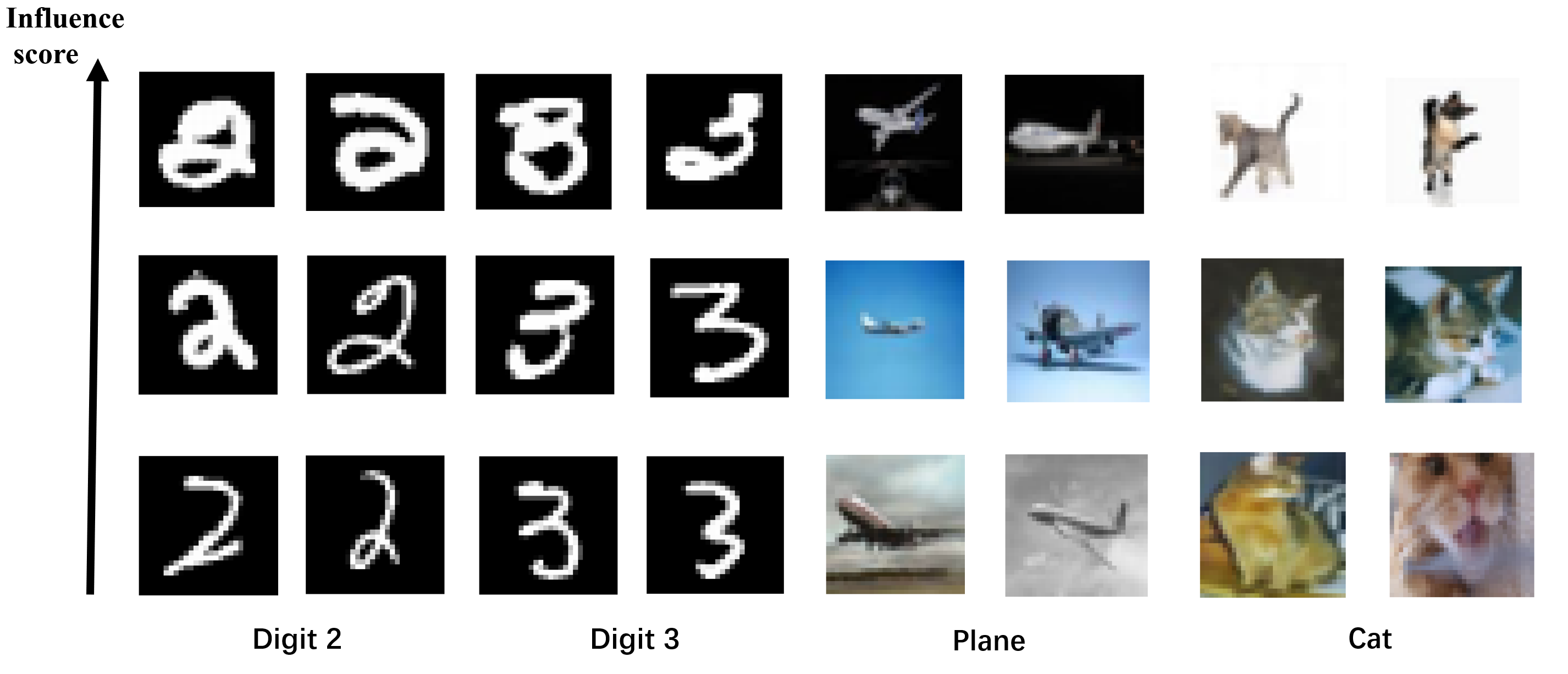
Figure 5: Visualization of images with different influence scores.

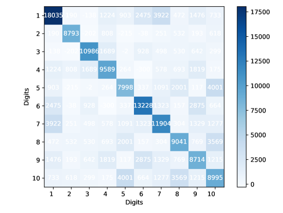
Figure 6: Visualization of the squared Frobenius norm among classes in MNIST.

5.2 Real-World Datasets

We verify the effects of noise correlation on MNIST (LeCun et al., 1998) and CIFAR-10 (Krizhevsky et al., 2009).

Noise correlation ratio verifications.

To verify our results in Theorem 1, we compute the squared Frobenius norm, i.e., $\|\mathbf{A}_{i}^{\top}\mathbf{A}_{j}\|_{F}$, among different classes in MNIST. As shown in Figure. 6, real datasets such as MNIST indeed have large noise correlation ratios, satisfying the conditions for long-tailed data benign overfitting predicted in our theory (Statement 2(b) of Theorem 1).

Data influence score.

We quantify the impact of a single data $(\mathbf{x},y)$ by measuring its impact on $\left\|\mathbf{A}_{y}^{\top}\mathbf{A}_{y}\right\|_{F}$ (A determining factor of the long-tailed data loss as in Statement 2(b) of Theorem 1). We observe that $\|\mathbf{A}_{y}^{\top}\mathbf{A}_{y}\|_{F}$ is, in fact, the same as the Frobenius norm of the covariance matrix of class $y$’s distribution and hence we consider an influence score of an image $(\mathbf{x},y)\in\mathcal{S}$ as

$$\text{infl}(\mathbf{x})=\left\|\hat{\Sigma}(\mathcal{S}_{y})\right\|_{F}^{2}-\left\|\hat{\Sigma}(\mathcal{S}_{y}\backslash\{\mathbf{x}\})\right\|_{F}^{2},$$ (10)

where $\hat{\Sigma}(\mathcal{S}_{y})$ denotes the estimated covariance of the underlying data distribution within the dataset $\mathcal{S}_{y}$.

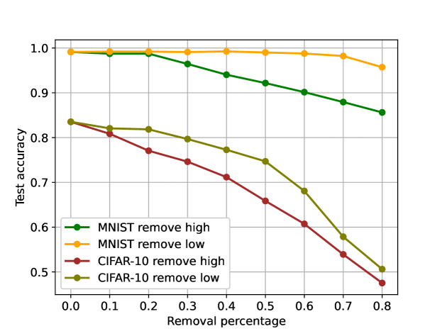
Figure 7: Effect on the test accuracy of removing a fraction of examples with high and low influence scores.

What influence scores indicate. We visualize the data with high and low influence scores in Figure 5. The data with high influence scores are atypical data, which can be interpreted by scrawly written digits and hard-to-classify objects in the experimental datasets.

Inspiration from influence scores. We sort the data from MNIST and CIFAR-10 based on the influence score defined in (10). In Figure 7, we remove a portion of data with high and low influence scores and train the remaining data on LeNet (LeCun et al., 1998) and ResNet-18 (He et al., 2016) to assess their impact on model accuracy. We observe that the accuracy drop of removing data with high influence scores is significantly larger than that of removing data with low influence scores. This observation verifies our theory (Statement 2(b) in Theorem 1) that reducing the squared Frobenius norm significantly hurts the model’s test performance as it reduces accuracy on long-tailed data.

6 Conclusions

In this paper, we rethink the overfitting phenomenon in overparameterized neural networks. Specifically, we enhance the widely used feature-noise data model by incorporating heterogeneous data noise across classes. Our findings reveal that neural networks can learn implicit features from data noise, previously deemed harmful, and leverage these features to enhance classification accuracy in long-tailed data distributions. These findings align with the practical observations that memorization can enhance generalization performance. Experiments on both synthetic and real-world datasets further validate our theory.

Appendix A Key lemmas

In this section, we present some important lemmas that illustrate the key properties of the data and neural networks.

Lemma 8.

Let $\mathbf{Z}\in\mathbb{R}^{m\times n}(m>n)$ be a matrix whose entries are independent and identically distributed Gaussian variables, i.e., $\mathbf{Z}_{i,j}\sim\mathcal{N}(0,1)$ for all $i\in[m],j\in[n]$. With probability at least $1-\delta$, all singular values of $\mathbf{Z}$, $\lambda_{i}(\mathbf{Z})$, for all $i\in[n]$ satisfies

$$\lambda_{i}(\mathbf{Z})\geq\sqrt{m}-2\sqrt{8\log(\mathchoice{\frac{2}{\delta}}{2/\delta}{2/\delta}{2/\delta})+8\log(9)n}.$$ (11)

Lemma 8 follows from the concentration inequality of Gaussian random matrices (Vershynin, 2018).

Lemma 9.

For $n$ random $\sigma_{p}$ sub-Gaussian variable $x_{1},\cdots,x_{n}$, with probability $1-\delta$, we have

$$\mathbb{P}[|x|\geq t]\leq 2\exp\left(-\mathchoice{\frac{t^{2}}{2\sigma_{p}^{2}}}{t^{2}/2\sigma_{p}^{2}}{t^{2}/2\sigma_{p}^{2}}{t^{2}/2\sigma_{p}^{2}}\right).$$ (12)

Proof.

Based on the definition of sub-Gaussian distribution, with probability of $1-\mathchoice{\frac{\delta}{n}}{\delta/n}{\delta/n}{\delta/n}$, we have

$$|x_{i}|\geq\sqrt{2\sigma_{p}^{2}\log(\mathchoice{\frac{2n}{\delta}}{2n/\delta}{2n/\delta}{2n/\delta})}.$$ (13)

By Union bound, we finishes the proof. ∎

Lemma 10.

Suppose two zero-mean random vectors $\mathbf{x},\mathbf{y}\in\mathbb{R}^{d}$ are generated as $\mathbf{x}=\mathbf{A}\boldsymbol{\zeta}_{1},\mathbf{y}=\mathbf{A}\boldsymbol{\zeta}_{2}$, where $\boldsymbol{\zeta}_{i}$’s each coordinate is independent, symmetric, and $\sigma_{p}$ sub-Gaussian with $\mathbb{E}[\zeta^{2}_{i,j}]=1$, for any $i\in[2],j\in[d]$. Then, $\mathbf{x}$ and $\mathbf{y}$ satisfy

$$\mathbb{P}\left[|\langle\mathbf{x},\mathbf{y}\rangle|\geq t\right]\leq 2\exp\left(-\Omega\left(\min\left\{\mathchoice{\frac{t^{2}}{\left\|\mathbf{A}^{\top}\mathbf{A}\right\|_{F}^{2}\sigma_{p}^{4}}}{t^{2}/\left\|\mathbf{A}^{\top}\mathbf{A}\right\|_{F}^{2}\sigma_{p}^{4}}{t^{2}/\left\|\mathbf{A}^{\top}\mathbf{A}\right\|_{F}^{2}\sigma_{p}^{4}}{t^{2}/\left\|\mathbf{A}^{\top}\mathbf{A}\right\|_{F}^{2}\sigma_{p}^{4}},\mathchoice{\frac{t}{\left\|\mathbf{A}^{\top}\mathbf{A}\right\|_{\textnormal{op}}\sigma^{2}_{p}}}{t/\left\|\mathbf{A}^{\top}\mathbf{A}\right\|_{\textnormal{op}}\sigma^{2}_{p}}{t/\left\|\mathbf{A}^{\top}\mathbf{A}\right\|_{\textnormal{op}}\sigma^{2}_{p}}{t/\left\|\mathbf{A}^{\top}\mathbf{A}\right\|_{\textnormal{op}}\sigma^{2}_{p}}\right\}\right)\right).$$ (14)

Proof.

We have

$$\left\langle\mathbf{x},\mathbf{y}\right\rangle=\left\langle\mathbf{A}\boldsymbol{\zeta}_{1},\mathbf{A}\boldsymbol{\zeta}_{2}\right\rangle=\boldsymbol{\zeta}_{1}^{\top}\mathbf{A}^{\top}\mathbf{A}\boldsymbol{\zeta}_{2}=\boldsymbol{\zeta}_{1}^{\top}\mathbf{U}^{\top}\Lambda\mathbf{U}\boldsymbol{\zeta}_{2}=\tilde{\boldsymbol{\zeta}}_{1}^{\top}\Lambda\tilde{\boldsymbol{\zeta}}_{2}=\mathrm{Tr}\left(\Lambda\tilde{\boldsymbol{\zeta}}_{2}\tilde{\boldsymbol{\zeta}}_{1}^{\top}\right).$$ (15)

As $\tilde{\boldsymbol{\zeta}}_{1}$ and $\tilde{\boldsymbol{\zeta}}_{2}$ are isotropic, by Bernstein’s inequality, we have

$$\mathbb{P}\left[\mathrm{Tr}\left(\Lambda\tilde{\boldsymbol{\zeta}}_{2}\tilde{\boldsymbol{\zeta}}_{1}^{\top}\right)\geq t\right]\leq 2\exp\left(-\Omega\left(\min\left\{\mathchoice{\frac{t^{2}}{\left\|\mathbf{A}^{\top}\mathbf{A}\right\|_{F}^{2}\sigma_{p}^{4}}}{t^{2}/\left\|\mathbf{A}^{\top}\mathbf{A}\right\|_{F}^{2}\sigma_{p}^{4}}{t^{2}/\left\|\mathbf{A}^{\top}\mathbf{A}\right\|_{F}^{2}\sigma_{p}^{4}}{t^{2}/\left\|\mathbf{A}^{\top}\mathbf{A}\right\|_{F}^{2}\sigma_{p}^{4}},\mathchoice{\frac{t}{\left\|\mathbf{A}^{\top}\mathbf{A}\right\|_{\text{op}}\sigma_{p}^{2}}}{t/\left\|\mathbf{A}^{\top}\mathbf{A}\right\|_{\text{op}}\sigma_{p}^{2}}{t/\left\|\mathbf{A}^{\top}\mathbf{A}\right\|_{\text{op}}\sigma_{p}^{2}}{t/\left\|\mathbf{A}^{\top}\mathbf{A}\right\|_{\text{op}}\sigma_{p}^{2}}\right\}\right)\right).$$ (16)

∎

Lemma 11.

Suppose a zero-mean random vector $\mathbf{x}\in\mathbb{R}^{d}$ is generated as $\mathbf{x}=\mathbf{A}\boldsymbol{\zeta}$, where $\boldsymbol{\zeta}$’s each coordinate is independent, symmetric, and $\sigma_{p}$ sub-Gaussian with $\mathbb{E}\left[\zeta^{2}_{j}\right]=1$, for any $j\in[d]$. Then, $\mathbf{x}$ satisfies

$$\mathbb{P}\left[\left\|\mathbf{x}\right\|_{2}^{2}-\mathrm{Tr}\left(\mathbf{A}^{\top}\mathbf{A}\right)\geq t\right]\leq 2\exp\left(-\Omega\left(\min\left\{\mathchoice{\frac{t^{2}}{\left\|\mathbf{A}^{\top}\mathbf{A}\right\|_{F}^{2}\sigma_{p}^{4}}}{t^{2}/\left\|\mathbf{A}^{\top}\mathbf{A}\right\|_{F}^{2}\sigma_{p}^{4}}{t^{2}/\left\|\mathbf{A}^{\top}\mathbf{A}\right\|_{F}^{2}\sigma_{p}^{4}}{t^{2}/\left\|\mathbf{A}^{\top}\mathbf{A}\right\|_{F}^{2}\sigma_{p}^{4}},\mathchoice{\frac{t}{\left\|\mathbf{A}^{\top}\mathbf{A}\right\|_{\textnormal{op}}\sigma_{p}^{2}}}{t/\left\|\mathbf{A}^{\top}\mathbf{A}\right\|_{\textnormal{op}}\sigma_{p}^{2}}{t/\left\|\mathbf{A}^{\top}\mathbf{A}\right\|_{\textnormal{op}}\sigma_{p}^{2}}{t/\left\|\mathbf{A}^{\top}\mathbf{A}\right\|_{\textnormal{op}}\sigma_{p}^{2}}\right\}\right)\right).$$ (17)

Proof.

We have

$$\left\|\mathbf{x}\right\|_{2}^{2}=\left\langle\mathbf{A}\boldsymbol{\zeta}_{1},\mathbf{A}\boldsymbol{\zeta}_{1}\right\rangle=\boldsymbol{\zeta}_{1}^{\top}\mathbf{A}^{\top}\mathbf{A}\boldsymbol{\zeta}_{1}=\mathrm{Tr}\left(\mathbf{A}^{\top}\mathbf{A}\boldsymbol{\zeta}_{1}\boldsymbol{\zeta}_{1}^{\top}\right).$$ (18)

Then, expectation of $\left\|\mathbf{x}\right\|_{2}$ satisfies

$$\mathbb{E}\left[\left\|\mathbf{x}\right\|_{2}^{2}\right]=\mathrm{Tr}\left(\mathbf{A}^{\top}\mathbf{A}\right).$$ (19)

By Bernstein’s inequality, we have

$$\mathbb{P}\left[\left\|\mathbf{x}\right\|_{2}^{2}-\mathrm{Tr}\left(\mathbf{A}^{\top}\mathbf{A}\right)\geq t\right]\leq 2\exp\left(-\Omega\left(\min\left\{\mathchoice{\frac{t^{2}}{\left\|\mathbf{A}^{\top}\mathbf{A}\right\|_{F}^{2}\sigma_{p}^{4}}}{t^{2}/\left\|\mathbf{A}^{\top}\mathbf{A}\right\|_{F}^{2}\sigma_{p}^{4}}{t^{2}/\left\|\mathbf{A}^{\top}\mathbf{A}\right\|_{F}^{2}\sigma_{p}^{4}}{t^{2}/\left\|\mathbf{A}^{\top}\mathbf{A}\right\|_{F}^{2}\sigma_{p}^{4}},\mathchoice{\frac{t}{\left\|\mathbf{A}^{\top}\mathbf{A}\right\|_{\text{op}}\sigma_{p}^{2}}}{t/\left\|\mathbf{A}^{\top}\mathbf{A}\right\|_{\text{op}}\sigma_{p}^{2}}{t/\left\|\mathbf{A}^{\top}\mathbf{A}\right\|_{\text{op}}\sigma_{p}^{2}}{t/\left\|\mathbf{A}^{\top}\mathbf{A}\right\|_{\text{op}}\sigma_{p}^{2}}\right\}\right)\right).$$ (20)

∎

Lemma 12.

Suppose two zero-mean random vectors $\mathbf{x}_{1},\mathbf{x}_{2}\in\mathbb{R}^{d}$ are generated as $\mathbf{x}_{1}=\mathbf{A}\boldsymbol{\zeta}_{1},\mathbf{x}_{2}=\mathbf{B}\boldsymbol{\zeta}_{2}$, where $\boldsymbol{\zeta}_{i}$’s each coordinate is independent, symmetric, and $\sigma_{p}$ sub-Gaussian with $\mathbb{E}[\zeta^{2}_{i,j}]=1$, for any $i\in[2],j\in[d]$. Then, $\mathbf{x}_{1}$ and $\mathbf{x}_{2}$ satisfy

$$\mathbb{P}\left[|\left\langle\mathbf{x}_{1},\mathbf{x}_{2}\right\rangle|\geq t\right]\leq 2\exp\left(-\Omega\left(\min\left\{\mathchoice{\frac{t^{2}}{\left\|\mathbf{A}^{\top}\mathbf{B}\right\|_{F}^{2}}}{t^{2}/\left\|\mathbf{A}^{\top}\mathbf{B}\right\|_{F}^{2}}{t^{2}/\left\|\mathbf{A}^{\top}\mathbf{B}\right\|_{F}^{2}}{t^{2}/\left\|\mathbf{A}^{\top}\mathbf{B}\right\|_{F}^{2}},\mathchoice{\frac{t}{\left\|\mathbf{A}^{\top}\mathbf{B}\right\|_{\textnormal{op}}}}{t/\left\|\mathbf{A}^{\top}\mathbf{B}\right\|_{\textnormal{op}}}{t/\left\|\mathbf{A}^{\top}\mathbf{B}\right\|_{\textnormal{op}}}{t/\left\|\mathbf{A}^{\top}\mathbf{B}\right\|_{\textnormal{op}}}\right\}\right)\right).$$ (21)

Proof.

We have

$$\left\langle\mathbf{x},\mathbf{y}\right\rangle=\left\langle\mathbf{A}\boldsymbol{\zeta}_{1},\mathbf{B}\boldsymbol{\zeta}_{2}\right\rangle=\boldsymbol{\zeta}_{1}^{\top}\mathbf{A}^{\top}\mathbf{B}\boldsymbol{\zeta}_{2}=\mathrm{Tr}\left(\mathbf{A}^{\top}\mathbf{B}\boldsymbol{\zeta}_{2}\boldsymbol{\zeta}_{1}^{\top}\right).$$ (22)

Then, by Bernstein’s inequality, we have

$$\mathbb{P}\left[|\left\langle\mathbf{x}_{1},\mathbf{x}_{2}\right\rangle|\geq t\right]= \mathbb{P}\left[\mathrm{Tr}\left(\mathbf{A}^{\top}\mathbf{B}\boldsymbol{\zeta}_{2}\boldsymbol{\zeta}_{1}^{\top}\right)\geq t\right]$$ (23)

$$\leq 2\exp\left(-\Omega\left(\min\left\{\mathchoice{\frac{t^{2}}{\left\|\mathbf{A}^{\top}\mathbf{B}\right\|_{F}^{2}\sigma_{p}^{4}}}{t^{2}/\left\|\mathbf{A}^{\top}\mathbf{B}\right\|_{F}^{2}\sigma_{p}^{4}}{t^{2}/\left\|\mathbf{A}^{\top}\mathbf{B}\right\|_{F}^{2}\sigma_{p}^{4}}{t^{2}/\left\|\mathbf{A}^{\top}\mathbf{B}\right\|_{F}^{2}\sigma_{p}^{4}},\mathchoice{\frac{t}{\left\|\mathbf{A}^{\top}\mathbf{B}\right\|_{\text{op}}\sigma_{p}^{2}}}{t/\left\|\mathbf{A}^{\top}\mathbf{B}\right\|_{\text{op}}\sigma_{p}^{2}}{t/\left\|\mathbf{A}^{\top}\mathbf{B}\right\|_{\text{op}}\sigma_{p}^{2}}{t/\left\|\mathbf{A}^{\top}\mathbf{B}\right\|_{\text{op}}\sigma_{p}^{2}}\right\}\right)\right).$$

∎

Lemma 13.

Let $x_{1},\cdots,x_{m}$ be $m$ independent zero-mean Gaussian variables. Denote $z_{i}$ as indicators for signs of $x_{i}$, i.e., for all $i\in[m]$,

$$z_{i}=\begin{cases}1,&x_{i}>0,\\ 0,&x_{i}\leq 0.\end{cases}$$ (24)

Then, we have

$$\Pr\left[\sum_{i=1}^{m}z_{i}\geq 0.4m\right]\geq 1-\exp\left(-\mathchoice{\frac{8}{25}}{8/25}{8/25}{8/25}m\right).$$ (25)

Proof.

Because $z_{i},i\in[m]$ are bounded in $[0,1]$, $z_{i},i\in[m]$ are sub-Gaussian variables. By Hoeffding’s inequality, we have

$$\Pr\left[m\left(\mathchoice{\frac{1}{m}}{1/m}{1/m}{1/m}\sum_{i=1}^{m}z_{i}\right)\leq m\left(\mathchoice{\frac{1}{2}}{1/2}{1/2}{1/2}-\epsilon\right)\right]\leq\exp\left(-\mathchoice{\frac{2m^{2}\epsilon^{2}}{m(\mathchoice{\frac{1}{16}}{1/16}{1/16}{1/16})}}{2m^{2}\epsilon^{2}/m(\mathchoice{\frac{1}{16}}{1/16}{1/16}{1/16})}{2m^{2}\epsilon^{2}/m(\mathchoice{\frac{1}{16}}{1/16}{1/16}{1/16})}{2m^{2}\epsilon^{2}/m(\mathchoice{\frac{1}{16}}{1/16}{1/16}{1/16})}\right).$$ (26)

Let $\epsilon=0.1$, we have

$$\Pr\left[\sum_{i=1}^{m}z_{i}\leq 0.4m\right]\leq\exp\left(-\mathchoice{\frac{8}{25}}{8/25}{8/25}{8/25}m\right).$$ (27)

Therefore, we have

$$\Pr\left[\sum_{i=1}^{m}z_{i}\geq 0.4m\right]\geq 1-\exp\left(-\mathchoice{\frac{8}{25}}{8/25}{8/25}{8/25}m\right).$$ (28)

This completes the proof. ∎

Lemma 14.

For any constant $t\in(0,1]$ and $x\in[-a,b],a,b>0$, we have

$$\log(1+t(\exp(x)-1))\leq\Gamma(x)x,$$ (29)

where $\Gamma(x)=\mathbb{I}(x\geq 0)+\left[\mathchoice{\frac{\log(1+t(\exp(-a)-1))}{-a}}{\log(1+t(\exp(-a)-1))/-a}{\log(1+t(\exp(-a)-1))/-a}{\log(1+t(\exp(-a)-1))/-a}\right]\mathbb{I}(x<0)$.

Proof.

First, considering $x\geq 0$, we have

$$\mathchoice{\frac{\partial\log(1+t(\exp(x)-1))}{\partial t}}{\partial\log(1+t(\exp(x)-1))/\partial t}{\partial\log(1+t(\exp(x)-1))/\partial t}{\partial\log(1+t(\exp(x)-1))/\partial t}= \mathchoice{\frac{\exp(x)-1}{1+t(\exp(x)-1)}}{\exp(x)-1/1+t(\exp(x)-1)}{\exp(x)-1/1+t(\exp(x)-1)}{\exp(x)-1/1+t(\exp(x)-1)}\geq 0.$$ (30)

Thus, $\log\left(1+t(\exp(x)-1)\right)\leq x,\forall x>0$. Second, considering $x<0$, we have

$$\mathchoice{\frac{\partial^{2}\log(1+t(\exp(x)-1))}{\partial x^{2}}}{\partial^{2}\log(1+t(\exp(x)-1))/\partial x^{2}}{\partial^{2}\log(1+t(\exp(x)-1))/\partial x^{2}}{\partial^{2}\log(1+t(\exp(x)-1))/\partial x^{2}}=\mathchoice{\frac{(1-t)t\exp(x)}{[1+t(\exp(x)-1)]^{2}}}{(1-t)t\exp(x)/[1+t(\exp(x)-1)]^{2}}{(1-t)t\exp(x)/[1+t(\exp(x)-1)]^{2}}{(1-t)t\exp(x)/[1+t(\exp(x)-1)]^{2}}\geq 0.$$ (31)

So $\log(1+t(\exp(x)-1))$ is a convex function of $x$. We can conclude that

$$\log(1+t(\exp(x)-1))\leq\mathchoice{\frac{\log(1+t(\exp(-a)-1))}{-a}}{\log(1+t(\exp(-a)-1))/-a}{\log(1+t(\exp(-a)-1))/-a}{\log(1+t(\exp(-a)-1))/-a}x,\forall x<0.$$ (32)

This completes the proof. ∎

Lemma 15.

With input $\mathbf{x}\in\mathbb{R}^{K}$, the function $f(\mathbf{x})=-\log(\mathchoice{\frac{\exp(x_{i})}{\sum_{j\in[K]}\exp(x_{j})}}{\exp(x_{i})/\sum_{j\in[K]}\exp(x_{j})}{\exp(x_{i})/\sum_{j\in[K]}\exp(x_{j})}{\exp(x_{i})/\sum_{j\in[K]}\exp(x_{j})})$ with any $i\in[K]$ is convex.

Proof.

For any $\mathbf{x}_{1},\mathbf{x}_{2}\in\mathbb{R}^{K}$ and $\alpha\in[0,1]$, we have

$$\alpha f(\mathbf{x}_{1})+(1-\alpha)f(\mathbf{x}_{2})= -\alpha\log\left(\mathchoice{\frac{\exp(x_{1,i})}{\sum_{j\in[K]}\exp(x_{1,j})}}{\exp(x_{1,i})/\sum_{j\in[K]}\exp(x_{1,j})}{\exp(x_{1,i})/\sum_{j\in[K]}\exp(x_{1,j})}{\exp(x_{1,i})/\sum_{j\in[K]}\exp(x_{1,j})}\right)-(1-\alpha)\log\left(\mathchoice{\frac{\exp(x_{2,i})}{\sum_{j\in[K]}\exp(x_{2,j})}}{\exp(x_{2,i})/\sum_{j\in[K]}\exp(x_{2,j})}{\exp(x_{2,i})/\sum_{j\in[K]}\exp(x_{2,j})}{\exp(x_{2,i})/\sum_{j\in[K]}\exp(x_{2,j})}\right)$$ (33)

$$= -\log\left(\left(\mathchoice{\frac{\exp(x_{1,i})}{\sum_{j\in[K]}\exp(x_{1,j})}}{\exp(x_{1,i})/\sum_{j\in[K]}\exp(x_{1,j})}{\exp(x_{1,i})/\sum_{j\in[K]}\exp(x_{1,j})}{\exp(x_{1,i})/\sum_{j\in[K]}\exp(x_{1,j})}\right)^{\alpha}\left(\mathchoice{\frac{\exp(x_{2,i})}{\sum_{j\in[K]}\exp(x_{2,j})}}{\exp(x_{2,i})/\sum_{j\in[K]}\exp(x_{2,j})}{\exp(x_{2,i})/\sum_{j\in[K]}\exp(x_{2,j})}{\exp(x_{2,i})/\sum_{j\in[K]}\exp(x_{2,j})}\right)^{1-\alpha}\right)$$

$$= -\log\left(\mathchoice{\frac{\exp(\alpha x_{1,i})}{(\sum_{j\in[K]}\exp(x_{1,j}))^{\alpha}}}{\exp(\alpha x_{1,i})/(\sum_{j\in[K]}\exp(x_{1,j}))^{\alpha}}{\exp(\alpha x_{1,i})/(\sum_{j\in[K]}\exp(x_{1,j}))^{\alpha}}{\exp(\alpha x_{1,i})/(\sum_{j\in[K]}\exp(x_{1,j}))^{\alpha}}\mathchoice{\frac{\exp((1-\alpha)x_{2,i})}{(\sum_{j\in[K]}\exp(x_{2,j}))^{1-\alpha}}}{\exp((1-\alpha)x_{2,i})/(\sum_{j\in[K]}\exp(x_{2,j}))^{1-\alpha}}{\exp((1-\alpha)x_{2,i})/(\sum_{j\in[K]}\exp(x_{2,j}))^{1-\alpha}}{\exp((1-\alpha)x_{2,i})/(\sum_{j\in[K]}\exp(x_{2,j}))^{1-\alpha}}\right)$$

$$= -\log\left(\mathchoice{\frac{\exp(\alpha x_{1,i}+(1-\alpha)x_{2,i})}{(\sum_{j\in[K]}\exp(x_{1,j}))^{\alpha}(\sum_{j\in[K]}\exp(x_{2,j}))^{1-\alpha}}}{\exp(\alpha x_{1,i}+(1-\alpha)x_{2,i})/(\sum_{j\in[K]}\exp(x_{1,j}))^{\alpha}(\sum_{j\in[K]}\exp(x_{2,j}))^{1-\alpha}}{\exp(\alpha x_{1,i}+(1-\alpha)x_{2,i})/(\sum_{j\in[K]}\exp(x_{1,j}))^{\alpha}(\sum_{j\in[K]}\exp(x_{2,j}))^{1-\alpha}}{\exp(\alpha x_{1,i}+(1-\alpha)x_{2,i})/(\sum_{j\in[K]}\exp(x_{1,j}))^{\alpha}(\sum_{j\in[K]}\exp(x_{2,j}))^{1-\alpha}}\right)$$

$$\geq -\log\left(\mathchoice{\frac{\exp(\alpha x_{1,i}+(1-\alpha)x_{2,i})}{\sum_{j\in[K]}\exp(\alpha x_{1,j}+(1-\alpha)x_{2,j})}}{\exp(\alpha x_{1,i}+(1-\alpha)x_{2,i})/\sum_{j\in[K]}\exp(\alpha x_{1,j}+(1-\alpha)x_{2,j})}{\exp(\alpha x_{1,i}+(1-\alpha)x_{2,i})/\sum_{j\in[K]}\exp(\alpha x_{1,j}+(1-\alpha)x_{2,j})}{\exp(\alpha x_{1,i}+(1-\alpha)x_{2,i})/\sum_{j\in[K]}\exp(\alpha x_{1,j}+(1-\alpha)x_{2,j})}\right)$$

$$= f(\alpha\mathbf{x}_{1}+(1-\alpha)\mathbf{x}_{2}).$$

This finishes the proof. ∎

Lemma 16.

A vector $\mathbf{z}$ uniformly sampled from $\mathbb{S}^{d-1}$ satisfies

$$\mathbb{P}\left[\left|\mathchoice{\frac{1}{d}}{1/d}{1/d}{1/d}\sum_{i=1}^{d}\mathbb{I}(z_{i})-\mathchoice{\frac{1}{2}}{1/2}{1/2}{1/2}\right|\geq t\right]\leq\exp\left(-2dt^{2}\right).$$ (34)

This lemma directly follows from Hoeffding’s inequality.

Lemma 17.

For a constant $0<t<1$, a $\sigma_{p}$ sub-Gaussian variable $x$ with variance 1 satisfies

$$\mathbb{P}\left[|x|>t\right]\geq\Omega((1-t^{2})^{2}).$$ (35)

Proof.

Since $x$ is a sub-Gaussian variable with variance 1, we have $\mathbb{E}[x]=1$. Applying Paley–Zygmund inequality to $x^{2}$, we have

$$\mathbb{P}[x^{2}\geq t]\geq(1-t)^{2}\mathchoice{\frac{1}{\mathbb{E}[x^{4}]}}{1/\mathbb{E}[x^{4}]}{1/\mathbb{E}[x^{4}]}{1/\mathbb{E}[x^{4}]}.$$ (36)

As the fourth moment of sub-Gaussian variable $\mathbb{E}[x^{4}]$ is bounded by $\mathcal{O}(\sigma_{p}^{4})$ (Vershynin, 2018), we have

$$\mathbb{P}[x^{2}\geq t]\geq\mathchoice{\frac{C_{4}}{\sigma_{p}^{4}}}{C_{4}/\sigma_{p}^{4}}{C_{4}/\sigma_{p}^{4}}{C_{4}/\sigma_{p}^{4}}(1-t)^{2},$$ (37)

where $C_{4}$ is a constant. This completes the proof. ∎

Lemma 18.

Let $\mathbf{A}\in\mathbb{R}^{m\times n}$ be a matrix with rank $M$. Suppose $\delta>0$ and $m\geq\Omega(\mathchoice{\frac{\log(\mathchoice{\frac{n}{\delta}}{n/\delta}{n/\delta}{n/\delta})(\lambda_{\max}^{+}(\mathbf{A}))^{2}}{((\lambda_{\min}^{+}(\mathbf{A}))^{2})}}{\log(\mathchoice{\frac{n}{\delta}}{n/\delta}{n/\delta}{n/\delta})(\lambda_{\max}^{+}(\mathbf{A}))^{2}/((\lambda_{\min}^{+}(\mathbf{A}))^{2})}{\log(\mathchoice{\frac{n}{\delta}}{n/\delta}{n/\delta}{n/\delta})(\lambda_{\max}^{+}(\mathbf{A}))^{2}/((\lambda_{\min}^{+}(\mathbf{A}))^{2})}{\log(\mathchoice{\frac{n}{\delta}}{n/\delta}{n/\delta}{n/\delta})(\lambda_{\max}^{+}(\mathbf{A}))^{2}/((\lambda_{\min}^{+}(\mathbf{A}))^{2})})$. With probability $1-\delta$, for any orthant $\mathcal{T}\in\mathbb{R}^{m}$ and vector $\mathbf{x}\in\mathbb{R}^{n}$ is a random sub-Gaussian vector with each coordinate follows $\mathcal{D}_{\xi}$, we have

$$\mathbb{P}\left[\mathbf{Ax}\in\mathcal{T}\right]\leq (0.6)^{M}.$$ (38)

Proof.

Using singular value decomposition for $\mathbf{A}$, for any orthant $\mathcal{T}\in\mathbb{R}^{m}$, we have

$$\mathbb{P}\left[\mathbf{Ax}\in\mathcal{T}\right]= \mathbb{P}\left[\mathbf{U}\mathbf{\Sigma}\mathbf{x}\in\mathcal{T}\right].$$ (39)

Without loss of generality, we assume the orthant $\mathcal{T}$ is that with all positive entries. Then, we have

$$\mathbb{P}\left[\mathbf{Ax}\in\mathcal{T}\right]\leq \mathbb{P}\left[\tilde{\mathbf{U}}\tilde{\mathbf{\Sigma}}\mathbf{x}\in\mathcal{T}\right],$$ (40)

where

$$\tilde{\mathbf{U}}=\begin{bmatrix}\mathbf{1}\cdot\mathchoice{\frac{1}{\sqrt{m}}}{1/\sqrt{m}}{1/\sqrt{m}}{1/\sqrt{m}}&\tilde{\mathbf{U}}_{2}&\cdots&\tilde{\mathbf{U}}_{m}\end{bmatrix},$$ (41)

and

$$\tilde{\mathbf{\Sigma}}=\begin{bmatrix}\lambda_{\max}^{+}(\mathbf{A})&0&\cdots&0&\\ 0&\lambda_{\min}^{+}(\mathbf{A})&\cdots&0&\\ \vdots&\vdots&&\vdots&\cdots\\ 0&0&\cdots&\lambda^{+}_{\min}(\mathbf{A})&\\ &&\cdots&&0\end{bmatrix},$$ (42)

Here, $\tilde{\mathbf{\Sigma}}$ is generated by replacing the non-zero singular values other than the largest one with $\lambda^{+}_{\min}(\mathbf{A})$. $\mathbf{1}$ is a vector with all one entries. In the following, we abbreviate $\lambda^{+}_{\max}(\mathbf{A})$ and $\lambda^{+}_{\min}(\mathbf{A})$ as $\lambda^{+}_{\max}$ and $\lambda^{+}_{\min}$ for convenience. Then, we have

$$\tilde{\mathbf{U}}\tilde{\mathbf{\Sigma}}\mathbf{x}=\lambda_{\max}^{+}\cdot\mathchoice{\frac{1}{\sqrt{m}}}{1/\sqrt{m}}{1/\sqrt{m}}{1/\sqrt{m}}\cdot\mathbf{1}\cdot x_{1}+\lambda_{\min}^{+}\sum_{i=2}^{M}x_{i}\tilde{\mathbf{U}}_{i}.$$ (43)

Here, as each coordinate of $\mathbf{x}$ is generate from $\mathcal{D}_{\xi}$, by Lemma 9, we have

$$|x_{i}|\leq\sqrt{2\sigma_{p}^{2}\log(\mathchoice{\frac{2n}{\delta}}{2n/\delta}{2n/\delta}{2n/\delta})},$$ (44)

with probability $1-\delta$. Then, we have

$$\mathbb{P}\left[\tilde{\mathbf{U}}\tilde{\mathbf{\Sigma}}\mathbf{x}\in\mathcal{T}\right]= \mathbb{P}\left[(\lambda_{\max}^{+}-\lambda_{\min}^{+})\cdot\mathchoice{\frac{1}{\sqrt{m}}}{1/\sqrt{m}}{1/\sqrt{m}}{1/\sqrt{m}}\cdot\mathbf{1}\cdot x_{1}+\lambda_{\min}^{+}\sum_{i=1}^{M}x_{i}\tilde{\mathbf{U}}_{i}\in\mathcal{T}\right]$$ (45)

$$\leq \mathbb{P}\left[\lambda_{\max}^{+}\cdot\mathchoice{\frac{1}{\sqrt{m}}}{1/\sqrt{m}}{1/\sqrt{m}}{1/\sqrt{m}}\cdot\mathbf{1}\cdot\sqrt{2\sigma_{p}^{2}\log(\mathchoice{\frac{2n}{\delta}}{2n/\delta}{2n/\delta}{2n/\delta})}+\lambda_{\min}^{+}\sum_{i=1}^{M}x_{i}\tilde{\mathbf{U}}_{i}\in\mathcal{T}\right]$$

$$= \mathbb{P}\left[\mathbf{1}\cdot\mathchoice{\frac{\sqrt{2\sigma_{p}^{2}\log(\mathchoice{\frac{2n}{\delta}}{2n/\delta}{2n/\delta}{2n/\delta})}\lambda^{+}_{\max}}{\sqrt{m}}}{\sqrt{2\sigma_{p}^{2}\log(\mathchoice{\frac{2n}{\delta}}{2n/\delta}{2n/\delta}{2n/\delta})}\lambda^{+}_{\max}/\sqrt{m}}{\sqrt{2\sigma_{p}^{2}\log(\mathchoice{\frac{2n}{\delta}}{2n/\delta}{2n/\delta}{2n/\delta})}\lambda^{+}_{\max}/\sqrt{m}}{\sqrt{2\sigma_{p}^{2}\log(\mathchoice{\frac{2n}{\delta}}{2n/\delta}{2n/\delta}{2n/\delta})}\lambda^{+}_{\max}/\sqrt{m}}+\lambda^{+}_{\min}\mathbf{x}\in\mathcal{T}\right].$$

As the entries of $\mathbf{x}$ are independent, we can bound each entry independently. Then, when $m\geq\Omega(\mathchoice{\frac{\log(\mathchoice{\frac{n}{\delta}}{n/\delta}{n/\delta}{n/\delta})(\lambda_{\max}^{+})^{2}}{((\lambda_{\min}^{+})^{2})}}{\log(\mathchoice{\frac{n}{\delta}}{n/\delta}{n/\delta}{n/\delta})(\lambda_{\max}^{+})^{2}/((\lambda_{\min}^{+})^{2})}{\log(\mathchoice{\frac{n}{\delta}}{n/\delta}{n/\delta}{n/\delta})(\lambda_{\max}^{+})^{2}/((\lambda_{\min}^{+})^{2})}{\log(\mathchoice{\frac{n}{\delta}}{n/\delta}{n/\delta}{n/\delta})(\lambda_{\max}^{+})^{2}/((\lambda_{\min}^{+})^{2})})$, we have

$$\mathbb{P}\left[\lambda_{\min}^{+}x_{i}+\mathchoice{\frac{\sqrt{2\sigma_{p}^{2}\log(\mathchoice{\frac{2n}{\delta}}{2n/\delta}{2n/\delta}{2n/\delta})}\lambda^{+}_{\max}}{\sqrt{m}}}{\sqrt{2\sigma_{p}^{2}\log(\mathchoice{\frac{2n}{\delta}}{2n/\delta}{2n/\delta}{2n/\delta})}\lambda^{+}_{\max}/\sqrt{m}}{\sqrt{2\sigma_{p}^{2}\log(\mathchoice{\frac{2n}{\delta}}{2n/\delta}{2n/\delta}{2n/\delta})}\lambda^{+}_{\max}/\sqrt{m}}{\sqrt{2\sigma_{p}^{2}\log(\mathchoice{\frac{2n}{\delta}}{2n/\delta}{2n/\delta}{2n/\delta})}\lambda^{+}_{\max}/\sqrt{m}}<0\right]\geq 0.4,$$ (46)

by the property of $\mathcal{D}_{\xi}$, resulting in

$$\mathbb{P}\left[\tilde{\mathbf{U}}\tilde{\mathbf{\Sigma}}\mathbf{x}\in\mathcal{T}\right]\leq (0.6)^{M}.$$ (47)

This completes the proof. ∎

Lemma 19.

Let $\mathbf{A}\in\mathbb{R}^{m\times n}$ be a matrix with rank $M$. Suppose $m\geq\Omega(\mathchoice{\frac{\log(\mathchoice{\frac{n}{\delta}}{n/\delta}{n/\delta}{n/\delta})(\lambda_{\max}^{+}(\mathbf{A}))^{2}}{((\lambda_{\min}^{+}(\mathbf{A}))^{2})}}{\log(\mathchoice{\frac{n}{\delta}}{n/\delta}{n/\delta}{n/\delta})(\lambda_{\max}^{+}(\mathbf{A}))^{2}/((\lambda_{\min}^{+}(\mathbf{A}))^{2})}{\log(\mathchoice{\frac{n}{\delta}}{n/\delta}{n/\delta}{n/\delta})(\lambda_{\max}^{+}(\mathbf{A}))^{2}/((\lambda_{\min}^{+}(\mathbf{A}))^{2})}{\log(\mathchoice{\frac{n}{\delta}}{n/\delta}{n/\delta}{n/\delta})(\lambda_{\max}^{+}(\mathbf{A}))^{2}/((\lambda_{\min}^{+}(\mathbf{A}))^{2})})$. With probability $1-\delta$, we have

$$\mathbb{P}\left[\sum_{i=1}^{m}\mathbb{I}((\mathbf{Ax})_{i}\leq 0)\geq 0.9m\right]\leq\exp(-0.07m).$$ (48)

Proof.

By Lemma 16, the number $N_{o}$ of orthants that have more than $0.9m$ negative entries satisfies

$$N_{o}\leq 2^{m}\cdot\exp(-0.32m)=\exp((\log 2-0.32)m).$$ (49)

Then, by Lemma 18, we have

$$\mathbb{P}\left[\sum_{i=1}^{m}\mathbb{I}((\mathbf{Ax})_{i}\leq 0)\geq 0.9m\right]\leq 0.6^{M}\cdot\exp((\log 2-0.32)m)$$ (50)

$$= \exp(\log(0.6)M+(\log 2-0.32)m)$$

$$\leq \exp(-0.51M+0.38m).$$

As long as $M\geq 0.9m$, we have

$$\mathbb{P}\left[\sum_{i=1}^{m}\mathbb{I}((\mathbf{Ax})_{i}\leq 0)\geq 0.9m\right]\leq \exp\left(-0.07m\right).$$ (51)

This completes the proof. ∎

Lemma 20.

Suppose that $\delta>0$ and $\mathrm{Tr}(\mathbf{A}_{i}^{\top}\mathbf{A}_{i})=\Omega\left(\max\left\{\left(\left\|\mathbf{A}^{\top}_{i}\mathbf{A}_{j}\right\|_{F}^{2}\sigma_{p}^{4}\log(\mathchoice{\frac{6n}{\delta}}{6n/\delta}{6n/\delta}{6n/\delta})\right)^{1/2},\left\|\mathbf{A}_{i}^{\top}\mathbf{A}_{j}\right\|_{\textnormal{op}}\sigma_{p}^{2}\log(\mathchoice{\frac{6n}{\delta}}{6n/\delta}{6n/\delta}{6n/\delta})\right\}\right)$. For all $i,j\in[K]$, with probability $1-\delta$, we have

$$\mathchoice{\frac{1}{2}}{1/2}{1/2}{1/2}\mathrm{Tr}(\mathbf{A}_{y_{i}}^{\top}\mathbf{A}_{y_{i}})\leq \left\|\boldsymbol{\xi}_{i}\right\|_{2}^{2}\leq\mathchoice{\frac{3}{2}}{3/2}{3/2}{3/2}\mathrm{Tr}(\mathbf{A}_{y_{i}}^{\top}\mathbf{A}_{y_{i}}),$$ (52)

$$|\langle\boldsymbol{\xi}_{i},\boldsymbol{\xi}_{j}\rangle|\leq \mathcal{O}\left(\max\left\{\left(\left\|\mathbf{A}_{y_{i}}^{\top}\mathbf{A}_{y_{j}}\right\|_{F}^{2}\log(\mathchoice{\frac{6n^{2}}{\delta}}{6n^{2}/\delta}{6n^{2}/\delta}{6n^{2}/\delta})\right)^{1/2},\left\|\mathbf{A}_{y_{i}}^{\top}\mathbf{A}_{y_{j}}\right\|_{\textnormal{op}}\log(\mathchoice{\frac{6n^{2}}{\delta}}{6n^{2}/\delta}{6n^{2}/\delta}{6n^{2}/\delta})\right\}\right).$$ (53)

Proof.

By Lemma 11, with probability at least $1-\mathchoice{\frac{\delta}{3n}}{\delta/3n}{\delta/3n}{\delta/3n}$, there exists a constant $C_{1}>0$ such that

$$\left\|\boldsymbol{\xi}_{i}\right\|_{2}^{2}\leq\mathrm{Tr}(\mathbf{A}_{y_{i}}^{\top}\mathbf{A}_{y_{i}})+\max\left\{\left(\left\|\mathbf{A}^{\top}_{y_{i}}\mathbf{A}_{y_{i}}\right\|_{F}^{2}\sigma_{p}^{4}\mathchoice{\frac{1}{C_{1}}}{1/C_{1}}{1/C_{1}}{1/C_{1}}\log(\mathchoice{\frac{6n}{\delta}}{6n/\delta}{6n/\delta}{6n/\delta})\right)^{1/2},\left\|\mathbf{A}_{y_{i}}^{\top}\mathbf{A}_{y_{i}}\right\|_{\text{op}}\sigma_{p}^{2}\mathchoice{\frac{1}{C_{1}}}{1/C_{1}}{1/C_{1}}{1/C_{1}}\log(\mathchoice{\frac{6n}{\delta}}{6n/\delta}{6n/\delta}{6n/\delta})\right\},$$

and

$$\left\|\boldsymbol{\xi}_{y_{i}}\right\|_{2}^{2}\geq\mathrm{Tr}(\mathbf{A}_{y_{i}}^{\top}\mathbf{A}_{y_{i}})-\max\left\{\left(\left\|\mathbf{A}_{y_{i}}^{\top}\mathbf{A}_{y_{i}}\right\|_{F}^{2}\sigma_{p}^{4}\mathchoice{\frac{1}{C_{1}}}{1/C_{1}}{1/C_{1}}{1/C_{1}}\log(\mathchoice{\frac{6n}{\delta}}{6n/\delta}{6n/\delta}{6n/\delta})\right)^{1/2},\left\|\mathbf{A}_{y_{i}}^{\top}\mathbf{A}_{y_{i}}\right\|_{\text{op}}\sigma_{p}^{2}\mathchoice{\frac{1}{C_{1}}}{1/C_{1}}{1/C_{1}}{1/C_{1}}\log(\mathchoice{\frac{6n}{\delta}}{6n/\delta}{6n/\delta}{6n/\delta})\right\}.$$

In addition, by Lemmas 12 and 10, with probability at least $1-\mathchoice{\frac{\delta}{3n^{2}}}{\delta/3n^{2}}{\delta/3n^{2}}{\delta/3n^{2}}$, there exists a constant $C_{2}>0$ such that

$$|\langle\boldsymbol{\xi}_{y_{i}},\boldsymbol{\xi}_{y_{j}}\rangle|\leq\max\left\{\left(\left\|\mathbf{A}_{y_{i}}^{\top}\mathbf{A}_{y_{j}}\right\|_{F}^{2}\sigma_{p}^{4}\mathchoice{\frac{1}{C_{2}}}{1/C_{2}}{1/C_{2}}{1/C_{2}}\log(\mathchoice{\frac{6n^{2}}{\delta}}{6n^{2}/\delta}{6n^{2}/\delta}{6n^{2}/\delta})\right)^{1/2},\left\|\mathbf{A}_{y_{i}}^{\top}\mathbf{A}_{y_{j}}\right\|_{\text{op}}\sigma_{p}^{2}\mathchoice{\frac{1}{C_{2}}}{1/C_{2}}{1/C_{2}}{1/C_{2}}\log(\mathchoice{\frac{6n^{2}}{\delta}}{6n^{2}/\delta}{6n^{2}/\delta}{6n^{2}/\delta})\right\}.$$

Applying $\sigma_{p}=\Theta(1)$ finishes the proof. ∎

Lemma 21.

Suppose that $d=\Omega(\log(\mathchoice{\frac{mn}{\delta}}{mn/\delta}{mn/\delta}{mn/\delta}))$ and $m=\Omega(\log(1/\delta))$. With probability at least $1-\delta$, for all $r\in[m],j\in[2],i\in[n]$,

$$|\langle\mathbf{w}_{j,r}^{(0)},\mathbf{u}_{k}\rangle|\leq\sqrt{2\log\left(\mathchoice{\frac{4Km}{\delta}}{4Km/\delta}{4Km/\delta}{4Km/\delta}\right)}\left\|\mathbf{u}_{k}\right\|_{2}\sigma_{0},$$ (54)

$$|\langle\mathbf{w}_{j,r}^{(0)},\boldsymbol{\xi}_{i}\rangle|\leq\mathcal{O}\left(\log\left(\mathchoice{\frac{Km}{\delta}}{Km/\delta}{Km/\delta}{Km/\delta}\right)\left\|\mathbf{A}_{y_{i}}\right\|_{F}\sigma_{0}\right).$$ (55)

Proof.

We prove the first bound (54) with Hoeffding’s inequality. For all $j\in[K],r\in[m],i\in[n]$, with probability $1-\mathchoice{\frac{\delta}{(2Km)}}{\delta/(2Km)}{\delta/(2Km)}{\delta/(2Km)}$,

$$|\langle\mathbf{w}_{j,r}^{(0)},\mathbf{u}_{k}\rangle|\leq\sqrt{2\log\left(\mathchoice{\frac{4Km}{\delta}}{4Km/\delta}{4Km/\delta}{4Km/\delta}\right)}\left\|\mathbf{u}_{k}\right\|_{2}\sigma_{0}.$$ (56)

Then, we prove the second bound (55) leveraging Lemma 12. For all $j\in[K],r\in[m],i\in[n]$, with probability $1-\mathchoice{\frac{\delta}{(2Km)}}{\delta/(2Km)}{\delta/(2Km)}{\delta/(2Km)}$,

$$|\langle\mathbf{w}^{(0)}_{j,r},\boldsymbol{\xi}_{i}\rangle|\leq \mathcal{O}\left(\max\left\{\sqrt{\log\left(\mathchoice{\frac{Km}{\delta}}{Km/\delta}{Km/\delta}{Km/\delta}\right)}\left\|\mathbf{A}_{y_{i}}\right\|_{F},\log\left(\mathchoice{\frac{Km}{\delta}}{Km/\delta}{Km/\delta}{Km/\delta}\right)\left\|\mathbf{A}_{y_{i}}\right\|_{\text{op}}\right\}\sigma_{0}\right)$$ (57)

$$\leq \mathcal{O}\left(\log\left(\mathchoice{\frac{Km}{\delta}}{Km/\delta}{Km/\delta}{Km/\delta}\right)\left\|\mathbf{A}_{y_{i}}\right\|_{F}\sigma_{0}\right).$$

∎

Lemma 22.

Suppose $\delta>0$ and $m\geq\Omega(\log(\mathchoice{\frac{n}{\delta}}{n/\delta}{n/\delta}{n/\delta}))$. With probability at least $1-\delta$, we have

$$|\mathcal{S}_{i}^{(0)}|\geq 0.4m.$$ (58)

Lemma 22 follows from Lemma 13 and union bound.

Lemma 23.

Suppose $\delta>0$ and $n\geq\Omega(\log(\mathchoice{\frac{m}{\delta}}{m/\delta}{m/\delta}{m/\delta}))$. For any neuron $\mathbf{w}_{j,r}^{(0)},j\in[2],r\in[m]$, with probability at least $1-\delta$, we have

$$\sum_{i=1}^{n}\mathbb{I}(\langle\mathbf{w}_{j,r}^{(0)},\boldsymbol{\xi}_{i}\rangle)\geq 0.4n.$$ (59)

Lemma 23 follows from Lemma 13 and union bound.

Appendix B Two-stage training loss analysis

In this section, we analyze the training loss. These results are based on the high probability conclusions in Appendix A. We divide the convergence of neural networks trained on each data into two stages. The training dynamics is at stage 1 at first and then enters stage 2 afterward. In Stage 1, we consider that the training data $(\mathbf{x},y)\in\mathcal{S}$ satisfies $1-\text{logit}_{y}(\mathbf{W},\mathbf{x})=\Theta(1)$.

B.1 Network gradient

The full-batch gradient on the neuron $\mathbf{w}_{k,r}$ at iteration $t$ is

$$\nabla_{\mathbf{w}_{k,r}^{(t)}}\mathcal{L}(\mathbf{W}^{(t)},\mathbf{x},y)= -\mathchoice{\frac{1}{mn}}{1/mn}{1/mn}{1/mn}\sum_{(\mathbf{x},y)\in\mathcal{S}}\left[\mathbb{I}\left(y=k\right)(1-\text{logit}_{k}(\mathbf{W}^{(t)},\mathbf{x}))\sum_{j=1}^{2}\sigma^{\prime}\left(\langle\mathbf{w}_{k,r}^{(t)},\mathbf{x}^{(j)}\rangle\right)\mathbf{x}^{(j)}\right]$$ (60)

$$+\mathchoice{\frac{1}{mn}}{1/mn}{1/mn}{1/mn}\sum_{(\mathbf{x},y)\in\mathcal{S}}\left[\mathbb{I}\left(y\neq k\right)\text{logit}_{k}(\mathbf{W}^{(t)},\mathbf{x})\sum_{j=1}^{2}\sigma^{\prime}\left(\langle\mathbf{w}_{k,r}^{(t)},\mathbf{x}^{(j)}\rangle\right)\mathbf{x}^{(j)}\right].$$

B.2 Training loss bounds at stage 1

First, we consider the training loss dynamics of stage 1 : For any data $(\mathbf{x},y)\in\mathcal{S}$, we have $\mathcal{L}(\mathbf{W}^{(t^{\prime})},\mathbf{x},y)=\Theta(1)$. First, we characterize the training loss.

$$\mathcal{L}(\mathbf{W}^{(t+1)},\mathbf{x},y)-\mathcal{L}(\mathbf{W}^{(t)},\mathbf{x},y)$$ (61)

$$= -\log\left(\text{prob}_{y}\left(\mathbf{W}^{(t+1)},\mathbf{x}\right)\right)+\log\left(\text{prob}_{y}\left(\mathbf{W}^{(t)},\mathbf{x}\right)\right)$$

$$= \log\left(\mathchoice{\frac{\text{prob}_{y}\left(\mathbf{W}^{(t)},\mathbf{x}\right)}{\text{prob}_{y}\left(\mathbf{W}^{(t+1)},\mathbf{x}\right)}}{\text{prob}_{y}\left(\mathbf{W}^{(t)},\mathbf{x}\right)/\text{prob}_{y}\left(\mathbf{W}^{(t+1)},\mathbf{x}\right)}{\text{prob}_{y}\left(\mathbf{W}^{(t)},\mathbf{x}\right)/\text{prob}_{y}\left(\mathbf{W}^{(t+1)},\mathbf{x}\right)}{\text{prob}_{y}\left(\mathbf{W}^{(t)},\mathbf{x}\right)/\text{prob}_{y}\left(\mathbf{W}^{(t+1)},\mathbf{x}\right)}\right)$$

$$= \log\left(\mathchoice{\frac{\mathchoice{\frac{\exp\left(F_{y}^{(t)}\left(\mathbf{x}\right)\right)}{\left(\exp\left(F_{y}^{(t)}\left(\mathbf{x}\right)\right)+\sum_{j\neq y}\exp\left(F_{j}^{(t)}\left(\mathbf{x}\right)\right)\right)}}{\exp\left(F_{y}^{(t)}\left(\mathbf{x}\right)\right)/\left(\exp\left(F_{y}^{(t)}\left(\mathbf{x}\right)\right)+\sum_{j\neq y}\exp\left(F_{j}^{(t)}\left(\mathbf{x}\right)\right)\right)}{\exp\left(F_{y}^{(t)}\left(\mathbf{x}\right)\right)/\left(\exp\left(F_{y}^{(t)}\left(\mathbf{x}\right)\right)+\sum_{j\neq y}\exp\left(F_{j}^{(t)}\left(\mathbf{x}\right)\right)\right)}{\exp\left(F_{y}^{(t)}\left(\mathbf{x}\right)\right)/\left(\exp\left(F_{y}^{(t)}\left(\mathbf{x}\right)\right)+\sum_{j\neq y}\exp\left(F_{j}^{(t)}\left(\mathbf{x}\right)\right)\right)}}{\mathchoice{\frac{\exp\left(F_{y}^{(t+1)}\left(\mathbf{x}\right)\right)}{\left(\exp\left(F_{y}^{(t+1)}\left(\mathbf{x}\right)\right)+\sum_{j\neq y}\exp\left(F_{j}^{(t+1)}\left(\mathbf{x}\right)\right)\right)}}{\exp\left(F_{y}^{(t+1)}\left(\mathbf{x}\right)\right)/\left(\exp\left(F_{y}^{(t+1)}\left(\mathbf{x}\right)\right)+\sum_{j\neq y}\exp\left(F_{j}^{(t+1)}\left(\mathbf{x}\right)\right)\right)}{\exp\left(F_{y}^{(t+1)}\left(\mathbf{x}\right)\right)/\left(\exp\left(F_{y}^{(t+1)}\left(\mathbf{x}\right)\right)+\sum_{j\neq y}\exp\left(F_{j}^{(t+1)}\left(\mathbf{x}\right)\right)\right)}{\exp\left(F_{y}^{(t+1)}\left(\mathbf{x}\right)\right)/\left(\exp\left(F_{y}^{(t+1)}\left(\mathbf{x}\right)\right)+\sum_{j\neq y}\exp\left(F_{j}^{(t+1)}\left(\mathbf{x}\right)\right)\right)}}}{\mathchoice{\frac{\exp\left(F_{y}^{(t)}\left(\mathbf{x}\right)\right)}{\left(\exp\left(F_{y}^{(t)}\left(\mathbf{x}\right)\right)+\sum_{j\neq y}\exp\left(F_{j}^{(t)}\left(\mathbf{x}\right)\right)\right)}}{\exp\left(F_{y}^{(t)}\left(\mathbf{x}\right)\right)/\left(\exp\left(F_{y}^{(t)}\left(\mathbf{x}\right)\right)+\sum_{j\neq y}\exp\left(F_{j}^{(t)}\left(\mathbf{x}\right)\right)\right)}{\exp\left(F_{y}^{(t)}\left(\mathbf{x}\right)\right)/\left(\exp\left(F_{y}^{(t)}\left(\mathbf{x}\right)\right)+\sum_{j\neq y}\exp\left(F_{j}^{(t)}\left(\mathbf{x}\right)\right)\right)}{\exp\left(F_{y}^{(t)}\left(\mathbf{x}\right)\right)/\left(\exp\left(F_{y}^{(t)}\left(\mathbf{x}\right)\right)+\sum_{j\neq y}\exp\left(F_{j}^{(t)}\left(\mathbf{x}\right)\right)\right)}/\mathchoice{\frac{\exp\left(F_{y}^{(t+1)}\left(\mathbf{x}\right)\right)}{\left(\exp\left(F_{y}^{(t+1)}\left(\mathbf{x}\right)\right)+\sum_{j\neq y}\exp\left(F_{j}^{(t+1)}\left(\mathbf{x}\right)\right)\right)}}{\exp\left(F_{y}^{(t+1)}\left(\mathbf{x}\right)\right)/\left(\exp\left(F_{y}^{(t+1)}\left(\mathbf{x}\right)\right)+\sum_{j\neq y}\exp\left(F_{j}^{(t+1)}\left(\mathbf{x}\right)\right)\right)}{\exp\left(F_{y}^{(t+1)}\left(\mathbf{x}\right)\right)/\left(\exp\left(F_{y}^{(t+1)}\left(\mathbf{x}\right)\right)+\sum_{j\neq y}\exp\left(F_{j}^{(t+1)}\left(\mathbf{x}\right)\right)\right)}{\exp\left(F_{y}^{(t+1)}\left(\mathbf{x}\right)\right)/\left(\exp\left(F_{y}^{(t+1)}\left(\mathbf{x}\right)\right)+\sum_{j\neq y}\exp\left(F_{j}^{(t+1)}\left(\mathbf{x}\right)\right)\right)}}{\mathchoice{\frac{\exp\left(F_{y}^{(t)}\left(\mathbf{x}\right)\right)}{\left(\exp\left(F_{y}^{(t)}\left(\mathbf{x}\right)\right)+\sum_{j\neq y}\exp\left(F_{j}^{(t)}\left(\mathbf{x}\right)\right)\right)}}{\exp\left(F_{y}^{(t)}\left(\mathbf{x}\right)\right)/\left(\exp\left(F_{y}^{(t)}\left(\mathbf{x}\right)\right)+\sum_{j\neq y}\exp\left(F_{j}^{(t)}\left(\mathbf{x}\right)\right)\right)}{\exp\left(F_{y}^{(t)}\left(\mathbf{x}\right)\right)/\left(\exp\left(F_{y}^{(t)}\left(\mathbf{x}\right)\right)+\sum_{j\neq y}\exp\left(F_{j}^{(t)}\left(\mathbf{x}\right)\right)\right)}{\exp\left(F_{y}^{(t)}\left(\mathbf{x}\right)\right)/\left(\exp\left(F_{y}^{(t)}\left(\mathbf{x}\right)\right)+\sum_{j\neq y}\exp\left(F_{j}^{(t)}\left(\mathbf{x}\right)\right)\right)}/\mathchoice{\frac{\exp\left(F_{y}^{(t+1)}\left(\mathbf{x}\right)\right)}{\left(\exp\left(F_{y}^{(t+1)}\left(\mathbf{x}\right)\right)+\sum_{j\neq y}\exp\left(F_{j}^{(t+1)}\left(\mathbf{x}\right)\right)\right)}}{\exp\left(F_{y}^{(t+1)}\left(\mathbf{x}\right)\right)/\left(\exp\left(F_{y}^{(t+1)}\left(\mathbf{x}\right)\right)+\sum_{j\neq y}\exp\left(F_{j}^{(t+1)}\left(\mathbf{x}\right)\right)\right)}{\exp\left(F_{y}^{(t+1)}\left(\mathbf{x}\right)\right)/\left(\exp\left(F_{y}^{(t+1)}\left(\mathbf{x}\right)\right)+\sum_{j\neq y}\exp\left(F_{j}^{(t+1)}\left(\mathbf{x}\right)\right)\right)}{\exp\left(F_{y}^{(t+1)}\left(\mathbf{x}\right)\right)/\left(\exp\left(F_{y}^{(t+1)}\left(\mathbf{x}\right)\right)+\sum_{j\neq y}\exp\left(F_{j}^{(t+1)}\left(\mathbf{x}\right)\right)\right)}}{\mathchoice{\frac{\exp\left(F_{y}^{(t)}\left(\mathbf{x}\right)\right)}{\left(\exp\left(F_{y}^{(t)}\left(\mathbf{x}\right)\right)+\sum_{j\neq y}\exp\left(F_{j}^{(t)}\left(\mathbf{x}\right)\right)\right)}}{\exp\left(F_{y}^{(t)}\left(\mathbf{x}\right)\right)/\left(\exp\left(F_{y}^{(t)}\left(\mathbf{x}\right)\right)+\sum_{j\neq y}\exp\left(F_{j}^{(t)}\left(\mathbf{x}\right)\right)\right)}{\exp\left(F_{y}^{(t)}\left(\mathbf{x}\right)\right)/\left(\exp\left(F_{y}^{(t)}\left(\mathbf{x}\right)\right)+\sum_{j\neq y}\exp\left(F_{j}^{(t)}\left(\mathbf{x}\right)\right)\right)}{\exp\left(F_{y}^{(t)}\left(\mathbf{x}\right)\right)/\left(\exp\left(F_{y}^{(t)}\left(\mathbf{x}\right)\right)+\sum_{j\neq y}\exp\left(F_{j}^{(t)}\left(\mathbf{x}\right)\right)\right)}/\mathchoice{\frac{\exp\left(F_{y}^{(t+1)}\left(\mathbf{x}\right)\right)}{\left(\exp\left(F_{y}^{(t+1)}\left(\mathbf{x}\right)\right)+\sum_{j\neq y}\exp\left(F_{j}^{(t+1)}\left(\mathbf{x}\right)\right)\right)}}{\exp\left(F_{y}^{(t+1)}\left(\mathbf{x}\right)\right)/\left(\exp\left(F_{y}^{(t+1)}\left(\mathbf{x}\right)\right)+\sum_{j\neq y}\exp\left(F_{j}^{(t+1)}\left(\mathbf{x}\right)\right)\right)}{\exp\left(F_{y}^{(t+1)}\left(\mathbf{x}\right)\right)/\left(\exp\left(F_{y}^{(t+1)}\left(\mathbf{x}\right)\right)+\sum_{j\neq y}\exp\left(F_{j}^{(t+1)}\left(\mathbf{x}\right)\right)\right)}{\exp\left(F_{y}^{(t+1)}\left(\mathbf{x}\right)\right)/\left(\exp\left(F_{y}^{(t+1)}\left(\mathbf{x}\right)\right)+\sum_{j\neq y}\exp\left(F_{j}^{(t+1)}\left(\mathbf{x}\right)\right)\right)}}\right)$$

$$= \log\left(\mathchoice{\frac{1+\sum_{j\neq y}\exp\left(F_{j}^{(t)}\left(\mathbf{x}\right)-F_{y}^{(t)}\left(\mathbf{x}\right)\right)\exp\left(\Delta_{j}^{(t)}\left(\mathbf{x}\right)-\Delta_{y}^{(t)}\left(\mathbf{x}\right)\right)}{1+\sum_{j\neq y}\exp\left(F_{j}^{(t)}\left(\mathbf{x}\right)-F_{y}^{(t)}\left(\mathbf{x}\right)\right)}}{1+\sum_{j\neq y}\exp\left(F_{j}^{(t)}\left(\mathbf{x}\right)-F_{y}^{(t)}\left(\mathbf{x}\right)\right)\exp\left(\Delta_{j}^{(t)}\left(\mathbf{x}\right)-\Delta_{y}^{(t)}\left(\mathbf{x}\right)\right)/1+\sum_{j\neq y}\exp\left(F_{j}^{(t)}\left(\mathbf{x}\right)-F_{y}^{(t)}\left(\mathbf{x}\right)\right)}{1+\sum_{j\neq y}\exp\left(F_{j}^{(t)}\left(\mathbf{x}\right)-F_{y}^{(t)}\left(\mathbf{x}\right)\right)\exp\left(\Delta_{j}^{(t)}\left(\mathbf{x}\right)-\Delta_{y}^{(t)}\left(\mathbf{x}\right)\right)/1+\sum_{j\neq y}\exp\left(F_{j}^{(t)}\left(\mathbf{x}\right)-F_{y}^{(t)}\left(\mathbf{x}\right)\right)}{1+\sum_{j\neq y}\exp\left(F_{j}^{(t)}\left(\mathbf{x}\right)-F_{y}^{(t)}\left(\mathbf{x}\right)\right)\exp\left(\Delta_{j}^{(t)}\left(\mathbf{x}\right)-\Delta_{y}^{(t)}\left(\mathbf{x}\right)\right)/1+\sum_{j\neq y}\exp\left(F_{j}^{(t)}\left(\mathbf{x}\right)-F_{y}^{(t)}\left(\mathbf{x}\right)\right)}\right)$$

$$= \log\left(1+\mathchoice{\frac{\sum_{j\neq y}\exp\left(F_{j}^{(t)}\left(\mathbf{x}\right)-F_{y}^{(t)}\left(\mathbf{x}\right)\right)\left(\exp\left(\Delta_{j}^{(t)}\left(\mathbf{x}\right)-\Delta_{y}^{(t)}\left(\mathbf{x}\right)\right)-1\right)}{1+\sum_{j\neq y}\exp\left(F_{j}^{(t)}\left(\mathbf{x}\right)-F_{y}^{(t)}\left(\mathbf{x}\right)\right)}}{\sum_{j\neq y}\exp\left(F_{j}^{(t)}\left(\mathbf{x}\right)-F_{y}^{(t)}\left(\mathbf{x}\right)\right)\left(\exp\left(\Delta_{j}^{(t)}\left(\mathbf{x}\right)-\Delta_{y}^{(t)}\left(\mathbf{x}\right)\right)-1\right)/1+\sum_{j\neq y}\exp\left(F_{j}^{(t)}\left(\mathbf{x}\right)-F_{y}^{(t)}\left(\mathbf{x}\right)\right)}{\sum_{j\neq y}\exp\left(F_{j}^{(t)}\left(\mathbf{x}\right)-F_{y}^{(t)}\left(\mathbf{x}\right)\right)\left(\exp\left(\Delta_{j}^{(t)}\left(\mathbf{x}\right)-\Delta_{y}^{(t)}\left(\mathbf{x}\right)\right)-1\right)/1+\sum_{j\neq y}\exp\left(F_{j}^{(t)}\left(\mathbf{x}\right)-F_{y}^{(t)}\left(\mathbf{x}\right)\right)}{\sum_{j\neq y}\exp\left(F_{j}^{(t)}\left(\mathbf{x}\right)-F_{y}^{(t)}\left(\mathbf{x}\right)\right)\left(\exp\left(\Delta_{j}^{(t)}\left(\mathbf{x}\right)-\Delta_{y}^{(t)}\left(\mathbf{x}\right)\right)-1\right)/1+\sum_{j\neq y}\exp\left(F_{j}^{(t)}\left(\mathbf{x}\right)-F_{y}^{(t)}\left(\mathbf{x}\right)\right)}\right)$$

$$\leq \log\left(1+\left(1-\text{prob}_{y}\left(\mathbf{W}^{(t)},\mathbf{x}\right)\right)\max_{j\neq y}\left(\exp\left(\Delta_{j}^{(t)}\left(\mathbf{x}\right)-\Delta_{y}^{(t)}\left(\mathbf{x}\right)\right)-1\right)\right),$$

where $\Delta_{y}^{(t)}\left(\mathbf{x}\right)=F_{y}^{(t+1)}\left(\mathbf{x}\right)-F_{y}^{(t)}\left(\mathbf{x}\right),\Delta_{j}^{(t)}\left(\mathbf{x}\right)=F_{j}^{(t+1)}\left(\mathbf{x}\right)-F_{j}^{(t)}\left(\mathbf{x}\right)$.

By Lemma 14, we have

$$\mathcal{L}\left(\mathbf{W}^{(t+1)},\mathbf{x},y\right)-\mathcal{L}\left(\mathbf{W}^{(t)},\mathbf{x},y\right)\leq\Theta(1)\cdot\max_{j\neq y}\left(\Delta_{j}^{(t)}(\mathbf{x})-\Delta_{y}^{(t)}(\mathbf{x})\right).$$ (62)

To measure how training loss changes over iterations, we need to characterize the change of $\Delta^{(t)}_{j}(\mathbf{x})-\Delta_{y}^{(t)}(\mathbf{x})$.

B.2.1 Upper bound of $\Delta_{j}^{(t)}(\mathbf{x})-\Delta_{y}^{(t)}(\mathbf{x})$

We first rearrange $\Delta_{j}^{(t)}(\mathbf{x})-\Delta_{y}^{(t)}(\mathbf{x})$ as follows.

$$\Delta_{j}^{(t)}\left(\mathbf{x}\right)-\Delta_{y}^{(t)}\left(\mathbf{x}\right)$$ (63)

$$= \mathchoice{\frac{1}{m}}{1/m}{1/m}{1/m}\sum_{r=1}^{m}\sum_{i=1}^{2}\left[\sigma\left(\left\langle\mathbf{w}^{(t+1)}_{j,r},\mathbf{x}^{(i)}\right\rangle\right)-\sigma\left(\left\langle\mathbf{w}^{(t)}_{j,r},\mathbf{x}^{(j)}\right\rangle\right)\right]$$

$$-\mathchoice{\frac{1}{m}}{1/m}{1/m}{1/m}\sum_{r=1}^{m}\sum_{i=1}^{2}\left[\sigma\left(\left\langle\mathbf{w}^{(t+1)}_{y,r},\mathbf{x}^{(i)}\right\rangle\right)-\sigma\left(\left\langle\mathbf{w}^{(t)}_{y,r},\mathbf{x}^{(i)}\right\rangle\right)\right]$$

$$= \underbrace{\mathchoice{\frac{1}{m}}{1/m}{1/m}{1/m}\sum_{r=1}^{m}\left[\sigma\left(\left\langle\mathbf{w}^{(t+1)}_{j,r},\mathbf{u}_{y}\right\rangle\right)-\sigma\left(\left\langle\mathbf{w}^{(t)}_{j,r},\mathbf{u}_{y}\right\rangle\right)\right]}_{A}\!+\!\underbrace{\mathchoice{\frac{1}{m}}{1/m}{1/m}{1/m}\sum_{r=1}^{m}\left[\sigma\left(\left\langle\mathbf{w}^{(t+1)}_{j,r},\boldsymbol{\xi}\right\rangle\right)-\sigma\left(\left\langle\mathbf{w}^{(t)}_{j,r},\boldsymbol{\xi}\right\rangle\right)\right]}_{B}$$

$$-\!\underbrace{\mathchoice{\frac{1}{m}}{1/m}{1/m}{1/m}\sum_{r=1}^{m}\left[\sigma\left(\left\langle\mathbf{w}^{(t+1)}_{y,r},\mathbf{u}_{y}\right\rangle\right)\!-\!\sigma\left(\left\langle\mathbf{w}^{(t)}_{y,r},\mathbf{u}_{y}\right\rangle\right)\right]}_{C}\!-\!\underbrace{\mathchoice{\frac{1}{m}}{1/m}{1/m}{1/m}\sum_{r=1}^{m}\left[\sigma\left(\left\langle\mathbf{w}^{(t+1)}_{y,r},\boldsymbol{\xi}\right\rangle\right)\!-\!\sigma\left(\left\langle\mathbf{w}^{(t)}_{y,r},\boldsymbol{\xi}\right\rangle\right)\right]}_{D},$$

We then bound $A,B,C,D$ in Stage 1.

Bound of $A$

$$A= \mathchoice{\frac{1}{m}}{1/m}{1/m}{1/m}\sum_{r=1}^{m}\left[\sigma\left(\langle\mathbf{w}_{j,r}^{(t)}\!-\!\mathchoice{\frac{\eta}{mn}}{\eta/mn}{\eta/mn}{\eta/mn}\sum_{(\mathbf{x}_{i},y_{i})\in\mathcal{S}_{y}}\sigma^{\prime}(\langle\mathbf{w}_{j,r}^{(t)},\mathbf{u}_{y}\rangle)\text{logit}_{j}(\mathbf{W}^{(t)},\mathbf{x}_{i})\mathbf{u}_{y},\mathbf{u}_{y}\rangle\right)\right]$$ (64)

$$-\mathchoice{\frac{1}{m}}{1/m}{1/m}{1/m}\sum_{r=1}^{m}\left[\sigma\left(\langle\mathbf{w}_{j,r}^{(t)},\mathbf{u}_{y}\rangle\right)\right]$$

$$\leq 0,$$

where the inequality is by the fact that $\langle\mathbf{u}_{y},\mathbf{u}_{y}\rangle\geq 0$.

Bound of $B$

$$B= \mathchoice{\frac{1}{m}}{1/m}{1/m}{1/m}\sum_{r=1}^{m}\left[\sigma\left(\left\langle\mathbf{w}_{j,r}^{(t)}-\mathchoice{\frac{\eta}{mn}}{\eta/mn}{\eta/mn}{\eta/mn}\sum_{(\mathbf{x}_{i},y_{i})\in\mathcal{S}\backslash\mathcal{S}_{j}}\sigma^{\prime}\left(\langle\mathbf{w}_{j,r}^{(t)},\boldsymbol{\xi}_{i}\rangle\right)\text{logit}_{j}(\mathbf{W}^{(t)},\mathbf{x}_{i})\boldsymbol{\xi}_{i}\right.\right.\right.$$ (65)

$$+\left.\left.\left.\mathchoice{\frac{\eta}{mn}}{\eta/mn}{\eta/mn}{\eta/mn}\sum_{(\mathbf{x}_{i},y_{i})\in\mathcal{S}_{j}}\sigma^{\prime}\left(\langle\mathbf{w}_{j,r}^{(t)},\boldsymbol{\xi}_{i}\rangle\right)\left(1-\text{logit}_{j}(\mathbf{W}^{(t)},\mathbf{x}_{i})\right)\boldsymbol{\xi}_{i},\boldsymbol{\xi}\right\rangle\right)\right]-\mathchoice{\frac{1}{m}}{1/m}{1/m}{1/m}\sum_{r=1}^{m}\left[\sigma\left(\langle\mathbf{w}_{j,r}^{(t)},\boldsymbol{\xi}\rangle\right)\right]$$

$$\leq \mathchoice{\frac{1}{m}}{1/m}{1/m}{1/m}\sum_{r=1}^{m}\left[\sigma\left(\left\langle\mathbf{w}_{j,r}^{(t)},\boldsymbol{\xi}\right\rangle-\mathchoice{\frac{\eta}{mn}}{\eta/mn}{\eta/mn}{\eta/mn}\sum_{(\mathbf{x}_{i},y_{i})\in\mathcal{S}\backslash\mathcal{S}_{j}}\sigma^{\prime}\left(\langle\mathbf{w}_{j,r}^{(t)},\boldsymbol{\xi}_{i}\rangle\right)\text{logit}_{j}(\mathbf{W}^{(t)},\mathbf{x}_{i})\boldsymbol{\xi}_{i}\right.\right.$$

$$+\left.\left.\left.\mathchoice{\frac{\eta}{mn}}{\eta/mn}{\eta/mn}{\eta/mn}\sum_{(\mathbf{x}_{i},y_{i})\in\mathcal{S}_{j}}\sigma^{\prime}\left(\langle\mathbf{w}_{j,r}^{(t)},\boldsymbol{\xi}_{i}\rangle\right)\left(1-\text{logit}_{j}(\mathbf{W}^{(t)},\mathbf{x}_{i})\right)\boldsymbol{\xi}_{i},\boldsymbol{\xi}\right\rangle\right)\right]-\mathchoice{\frac{1}{m}}{1/m}{1/m}{1/m}\sum_{r=1}^{m}\left[\sigma\left(\langle\mathbf{w}_{j,r}^{(t)},\boldsymbol{\xi}\rangle\right)\right]$$

$$\leq \mathchoice{\frac{\eta}{mn}}{\eta/mn}{\eta/mn}{\eta/mn}\sum_{(\mathbf{x}_{i},y_{i})\in\mathcal{S}\backslash\mathcal{S}_{j}}\sigma^{\prime}\left(\langle\mathbf{w}_{j,r}^{(t)},\boldsymbol{\xi}_{i}\rangle\right)\text{logit}_{j}(\mathbf{W}^{(t)},\mathbf{x}_{i})|\langle\boldsymbol{\xi}_{i},\boldsymbol{\xi}\rangle|$$

$$+\mathchoice{\frac{\eta}{mn}}{\eta/mn}{\eta/mn}{\eta/mn}\sum_{(\mathbf{x}_{i},y_{i})\in\mathcal{S}_{j}\backslash(\mathbf{x},y)}\sigma^{\prime}\left(\langle\mathbf{w}_{j,r}^{(t)},\boldsymbol{\xi}_{i}\rangle\right)\left(1-\text{logit}_{j}(\mathbf{W}^{(t)},\mathbf{x}_{i})\right)|\langle\boldsymbol{\xi}_{i},\boldsymbol{\xi}\rangle|,$$

where the inequality is by the 1-Lipschitz property of the ReLU function.

Bound of $C$

$$C= \mathchoice{\frac{1}{m}}{1/m}{1/m}{1/m}\sum_{r=1}^{m}\left[\sigma\left(\left\langle\mathbf{w}_{y,r}^{(t)}+\mathchoice{\frac{\eta}{mn}}{\eta/mn}{\eta/mn}{\eta/mn}\sum_{(\mathbf{x}_{i},y_{i})\in\mathcal{S}_{y}}\sigma^{\prime}(\langle\mathbf{w}_{y,r}^{(t)},\mathbf{u}_{y}\rangle)\left(1-\text{logit}_{y}(\mathbf{W}^{(t)},\mathbf{x}_{i})\right)\mathbf{u}_{y},\mathbf{u}_{y}\right\rangle\right)\right]$$ (66)

$$-\mathchoice{\frac{1}{m}}{1/m}{1/m}{1/m}\sum_{r=1}^{m}\left[\sigma\left(\langle\mathbf{w}_{y,r}^{(t)},\mathbf{u}_{y}\rangle\right)\right]$$

$$\geq \mathchoice{\frac{2\eta}{5mn}}{2\eta/5mn}{2\eta/5mn}{2\eta/5mn}\sum_{(\mathbf{x},y)\in\mathcal{S}_{y}}\left(1-\text{logit}_{y}(\mathbf{W}^{(t)},\mathbf{x}_{i})\right)\left\|\mathbf{u}_{y}\right\|_{2}^{2},$$

where the inequality is by the fact that $\left\|\mathbf{u}_{y}\right\|_{2}^{2}\geq 0$.

Bound of $D$

$$D= \mathchoice{\frac{1}{m}}{1/m}{1/m}{1/m}\sum_{r=1}^{m}\left[\sigma\left(\left\langle\mathbf{w}_{y,r}^{(t)}-\mathchoice{\frac{\eta}{mn}}{\eta/mn}{\eta/mn}{\eta/mn}\sum_{(\mathbf{x}_{i},y_{i})\in\mathcal{S}\backslash\mathcal{S}_{y}}\sigma^{\prime}(\langle\mathbf{w}_{y,r}^{(t)},\boldsymbol{\xi}_{i}\rangle)\text{logit}_{y}(\mathbf{W}^{(t)},\mathbf{x}_{i})\boldsymbol{\xi}_{i}\right.\right.\right.$$ (67)

$$+\left.\left.\left.\mathchoice{\frac{\eta}{mn}}{\eta/mn}{\eta/mn}{\eta/mn}\sum_{(\mathbf{x}_{i},y_{i})\in\mathcal{S}_{y}}\sigma^{\prime}\left(\langle\mathbf{w}_{y,r}^{(t)},\boldsymbol{\xi}_{i}\rangle\right)\left(1-\text{logit}_{y}(\mathbf{W}^{(t)},\mathbf{x}_{i})\right)\boldsymbol{\xi}_{i},\boldsymbol{\xi}\right\rangle\right)\right]$$

$$-\mathchoice{\frac{1}{m}}{1/m}{1/m}{1/m}\sum_{r=1}^{m}\left[\sigma\left(\langle\mathbf{w}_{y,r}^{(t)},\boldsymbol{\xi}\rangle\right)\right]$$

$$\geq \mathchoice{\frac{1}{m}}{1/m}{1/m}{1/m}\sum_{r=1}^{m}\left[\sigma\left(\left\langle\mathbf{w}_{y,r}^{(t)},\boldsymbol{\xi}\right\rangle-\mathchoice{\frac{\eta}{mn}}{\eta/mn}{\eta/mn}{\eta/mn}\sum_{(\mathbf{x}_{i},y_{i})\in\mathcal{S}\backslash\mathcal{S}_{y}}\sigma^{\prime}(\langle\mathbf{w}_{y,r}^{(t)},\boldsymbol{\xi}_{i}\rangle)\text{logit}_{y}(\mathbf{W}^{(t)},\mathbf{x}_{i})|\left\langle\boldsymbol{\xi}_{i},\boldsymbol{\xi}\right\rangle|\right.\right.$$

$$+\mathchoice{\frac{\eta}{mn}}{\eta/mn}{\eta/mn}{\eta/mn}\sigma^{\prime}\left(\langle\mathbf{w}_{y,r}^{(t)},\boldsymbol{\xi}\rangle\right)\left(1-\text{logit}_{y}(\mathbf{W}^{(t)},\mathbf{x})\right)\left\|\boldsymbol{\xi}\right\|_{2}^{2}$$

$$-\left.\left.\mathchoice{\frac{\eta}{mn}}{\eta/mn}{\eta/mn}{\eta/mn}\sum_{(\mathbf{x}_{i},y_{i})\in\mathcal{S}_{y}\backslash(\mathbf{x},y)}\sigma^{\prime}\left(\langle\mathbf{w}_{y,r}^{(t)},\boldsymbol{\xi}_{i}\rangle\right)\left(1-\text{logit}_{y}(\mathbf{W}^{(t)},\mathbf{x}_{i})\right)|\left\langle\boldsymbol{\xi}_{i},\boldsymbol{\xi}\right\rangle|\right)\right]$$

$$-\mathchoice{\frac{1}{m}}{1/m}{1/m}{1/m}\sum_{r=1}^{m}\left[\sigma\left(\langle\mathbf{w}_{y,r}^{(t)},\boldsymbol{\xi}_{j}\rangle\right)\right]$$

$$\geq -\mathchoice{\frac{\eta}{mn}}{\eta/mn}{\eta/mn}{\eta/mn}\sum_{(\mathbf{x}_{i},y_{i})\in\mathcal{S}\backslash\mathcal{S}_{y}}\text{logit}_{y}(\mathbf{W}^{(t)},\mathbf{x}_{i})|\left\langle\boldsymbol{\xi}_{i},\boldsymbol{\xi}\right\rangle|+\mathchoice{\frac{2\eta}{5mn}}{2\eta/5mn}{2\eta/5mn}{2\eta/5mn}\left(1-\text{logit}_{y}(\mathbf{W}^{(t)},\mathbf{x})\right)\left\|\boldsymbol{\xi}\right\|_{2}^{2}$$

$$-\mathchoice{\frac{\eta}{mn}}{\eta/mn}{\eta/mn}{\eta/mn}\sum_{(\mathbf{x}_{i},y_{i})\in\mathcal{S}_{y}\backslash(\mathbf{x},y)}\left(1-\text{logit}_{y}(\mathbf{W}^{(t)},\mathbf{x}_{i})\right)|\left\langle\boldsymbol{\xi}_{i},\boldsymbol{\xi}\right\rangle|$$

$$\geq 0,$$

where the last inequality is by that fact that the incremental term is larger than zero if a neuron is activated, by Lemmas 7, 22, at least 0.4$m$ neurons are activated, and $\sigma^{\prime}(\cdot)\leq 1$.

Substituting $(\ref{equ: bound_A}),(\ref{equ: bound_B}),(\ref{equ: bound_C}),(\ref{equ: bound_D})$ into $(\ref{equ: delta})$, by Lemma 20 and Condition 1, we have

$$\Delta_{j}^{(t)}(\mathbf{x})-\Delta_{y}^{(t)}(\mathbf{x})$$ (68)

$$\leq -\mathchoice{\frac{2\eta}{5mn}}{2\eta/5mn}{2\eta/5mn}{2\eta/5mn}\sum_{(\mathbf{x},y)\in\mathcal{S}_{y}}\left(1-\text{logit}_{y}(\mathbf{W}^{(t)},\mathbf{x}_{i})\right)\left\|\mathbf{u}_{y}\right\|_{2}^{2}$$

$$+\mathchoice{\frac{2\eta}{mn}}{2\eta/mn}{2\eta/mn}{2\eta/mn}\sum_{(\mathbf{x}_{i},y_{i})\in\mathcal{S}\backslash\mathcal{S}_{y}}\text{logit}_{y}(\mathbf{W}^{(t)},\mathbf{x}_{i})|\left\langle\boldsymbol{\xi}_{i},\boldsymbol{\xi}\right\rangle|-\mathchoice{\frac{2\eta}{5mn}}{2\eta/5mn}{2\eta/5mn}{2\eta/5mn}\left(1-\text{logit}_{y}(\mathbf{W}^{(t)},\mathbf{x})\right)\left\|\boldsymbol{\xi}\right\|_{2}^{2}$$

$$+\mathchoice{\frac{2\eta}{mn}}{2\eta/mn}{2\eta/mn}{2\eta/mn}\sum_{(\mathbf{x}_{i},y_{i})\in\mathcal{S}_{y}\backslash(\mathbf{x},y)}\left(1-\text{logit}_{y}(\mathbf{W}^{(t)},\mathbf{x}_{i})\right)|\left\langle\boldsymbol{\xi}_{i},\boldsymbol{\xi}\right\rangle|$$

$$\leq -\mathchoice{\frac{2\eta}{5mn}}{2\eta/5mn}{2\eta/5mn}{2\eta/5mn}\sum_{(\mathbf{x},y)\in\mathcal{S}_{y}}\left(1-\text{logit}_{y}(\mathbf{W}^{(t)},\mathbf{x}_{i})\right)\left\|\mathbf{u}_{y}\right\|_{2}^{2}.$$

Combining $(\ref{equ: delta_total})$ and $(\ref{equ: loss_increment})$, for any $(\mathbf{x},y)\in\mathcal{S}$ we have

$$\mathcal{L}(\mathbf{W}^{(t+1)},\mathbf{x},y)\leq \mathcal{L}(\mathbf{W}^{(t)},\mathbf{x},y)-\mathchoice{\frac{2\eta}{5mn}}{2\eta/5mn}{2\eta/5mn}{2\eta/5mn}\sum_{(\mathbf{x}_{i},y_{i})\in\mathcal{S}_{y}}\left(1-\text{logit}_{y}(\mathbf{W}^{(t)},\mathbf{x}_{i})\right)\left\|\mathbf{u}_{y}\right\|_{2}^{2}$$ (69)

$$\overset{(a)}{=} \left(1-\Theta\left(\mathchoice{\frac{\eta}{mn}}{\eta/mn}{\eta/mn}{\eta/mn}|\mathcal{S}_{y}|\left\|\mathbf{u}_{y}\right\|_{2}^{2}\right)\right)\mathcal{L}(\mathbf{W}^{(t)},\mathbf{x},y),$$

where $(a)$ is obtained from Lemma 7. This finishes the training loss analysis in Stage 1.

B.2.2 Analysis of stage 2

In stage 2, the loss of certain data is no longer $\Theta(1)$.

First, let $\mathbf{W}^{*}$ be

$$\mathbf{w}_{j,r}^{*}=2.5\log\left(\mathchoice{\frac{4(K-1)}{\epsilon}}{4(K-1)/\epsilon}{4(K-1)/\epsilon}{4(K-1)/\epsilon}\right)\mathchoice{\frac{\mathbf{u}_{j}}{\left\|\mathbf{u}_{j}\right\|_{2}^{2}}}{\mathbf{u}_{j}/\left\|\mathbf{u}_{j}\right\|_{2}^{2}}{\mathbf{u}_{j}/\left\|\mathbf{u}_{j}\right\|_{2}^{2}}{\mathbf{u}_{j}/\left\|\mathbf{u}_{j}\right\|_{2}^{2}},$$ (70)

where $\epsilon>0$ is a small constant. We have

$$\left\|\mathbf{W}^{(t)}-\mathbf{W}^{*}\right\|_{F}^{2}-\left\|\mathbf{W}^{(t+1)}-\mathbf{W}^{*}\right\|_{F}^{2}=\underbrace{2\eta\left\langle\nabla\mathcal{L}_{S}(\mathbf{W}^{(t)}),\mathbf{W}^{(t)}-\mathbf{W}^{*}\right\rangle}_{A}-\underbrace{\eta^{2}\left\|\nabla\mathcal{L}_{S}(\mathbf{W}^{(t)})\right\|_{F}^{2}}_{B}.$$ (71)

For the first term $A$, we have

$$A= 2\eta\left\langle\nabla\mathcal{L}_{S}(\mathbf{W}^{(t)}),\mathbf{W}^{(t)}-\mathbf{W}^{*}\right\rangle$$ (72)

$$= \mathchoice{\frac{2\eta}{n}}{2\eta/n}{2\eta/n}{2\eta/n}\sum_{(\mathbf{x},y)\in\mathcal{S}}\left\langle\nabla\mathcal{L}(\mathbf{W}^{(t)},\mathbf{x},y),\mathbf{W}^{(t)}-\mathbf{W}^{*}\right\rangle$$

$$= \mathchoice{\frac{2\eta}{n}}{2\eta/n}{2\eta/n}{2\eta/n}\sum_{(\mathbf{x},y)\in\mathcal{S}}\sum_{k\in[K]}\left\langle\mathchoice{\frac{\partial\mathcal{L}(\mathbf{W}^{(t)},\mathbf{x},y)}{\partial F_{k}}}{\partial\mathcal{L}(\mathbf{W}^{(t)},\mathbf{x},y)/\partial F_{k}}{\partial\mathcal{L}(\mathbf{W}^{(t)},\mathbf{x},y)/\partial F_{k}}{\partial\mathcal{L}(\mathbf{W}^{(t)},\mathbf{x},y)/\partial F_{k}}\nabla F_{k}(\mathbf{W}^{(t)},\mathbf{x},y),\mathbf{W}^{(t)}-\mathbf{W}^{*}\right\rangle$$

$$= \mathchoice{\frac{2\eta}{n}}{2\eta/n}{2\eta/n}{2\eta/n}\sum_{(\mathbf{x},y)\in\mathcal{S}}\sum_{k\in[K]}\mathchoice{\frac{\partial\mathcal{L}(\mathbf{W}^{(t)},\mathbf{x},y)}{\partial F_{k}}}{\partial\mathcal{L}(\mathbf{W}^{(t)},\mathbf{x},y)/\partial F_{k}}{\partial\mathcal{L}(\mathbf{W}^{(t)},\mathbf{x},y)/\partial F_{k}}{\partial\mathcal{L}(\mathbf{W}^{(t)},\mathbf{x},y)/\partial F_{k}}\left\langle\nabla F_{k}(\mathbf{W}^{(t)},\mathbf{x},y),\mathbf{W}^{(t)}\right\rangle$$

$$-\mathchoice{\frac{2\eta}{n}}{2\eta/n}{2\eta/n}{2\eta/n}\sum_{(\mathbf{x},y)\in\mathcal{S}}\sum_{k\in[K]}\mathchoice{\frac{\partial\mathcal{L}(\mathbf{W}^{(t)},\mathbf{x},y)}{\partial F_{k}}}{\partial\mathcal{L}(\mathbf{W}^{(t)},\mathbf{x},y)/\partial F_{k}}{\partial\mathcal{L}(\mathbf{W}^{(t)},\mathbf{x},y)/\partial F_{k}}{\partial\mathcal{L}(\mathbf{W}^{(t)},\mathbf{x},y)/\partial F_{k}}\left\langle\nabla F_{k}(\mathbf{W}^{(t)},\mathbf{x},y),\mathbf{W}^{*}\right\rangle$$

$$= \mathchoice{\frac{2\eta}{n}}{2\eta/n}{2\eta/n}{2\eta/n}\sum_{(\mathbf{x},y)\in\mathcal{S}}\sum_{k\in[K]}\mathchoice{\frac{\partial\mathcal{L}(\mathbf{W}^{(t)},\mathbf{x},y)}{\partial F_{k}}}{\partial\mathcal{L}(\mathbf{W}^{(t)},\mathbf{x},y)/\partial F_{k}}{\partial\mathcal{L}(\mathbf{W}^{(t)},\mathbf{x},y)/\partial F_{k}}{\partial\mathcal{L}(\mathbf{W}^{(t)},\mathbf{x},y)/\partial F_{k}}\left(F_{k}(\mathbf{W}^{(t)},\mathbf{x},y)-\underbrace{\left\langle\nabla F_{k}(\mathbf{W}^{(t)},\mathbf{x},y),\mathbf{W}^{*}\right\rangle}_{C}\right),$$

where the last equality is based on the homogeneity of $F_{k}(\cdot)$ for any $k\in[K]$. Then, we need to bound $C$. First, for any $i,k\in[K]$, we have

$$\nabla_{\mathbf{w}_{k,r}^{(t)}}F_{i}(\mathbf{W}^{(t)},\mathbf{x},y)= \mathchoice{\frac{1}{m}}{1/m}{1/m}{1/m}\left(\sigma^{\prime}\left(\left\langle\mathbf{w}_{k,r}^{(t)},\boldsymbol{\xi}\right\rangle\right)\boldsymbol{\xi}+\sigma^{\prime}\left(\left\langle\mathbf{w}_{k,r}^{(t)},\mathbf{u}_{y}\right\rangle\right)\mathbf{u}_{y}\right)\mathbb{I}(k=i).$$ (73)

By the definition of $\mathbf{W}^{*}$ in (70), we can get the components of $C$ as

$$\left\langle\nabla F_{i}(\mathbf{W}^{(t)},\mathbf{x},y),\mathbf{W}^{*}\right\rangle=\begin{cases}\frac{2.5\log\left(\mathchoice{\frac{4(K-1)}{\epsilon}}{4(K-1)/\epsilon}{4(K-1)/\epsilon}{4(K-1)/\epsilon}\right)}{m}\sum_{r=1}^{m}\sigma^{\prime}\left(\left\langle\mathbf{w}_{i,r}^{(t)},\mathbf{u}_{y}\right\rangle\right)\left\|\mathbf{u}_{y}\right\|_{2}^{2}&\text{if }i=y,\\ 0&\text{if }i\neq y.\end{cases}$$ (74)

Next, we bound $B$.

$$B= \eta^{2}\left\|\nabla\mathcal{L}_{S}(\mathbf{W}^{(t)})\right\|_{F}^{2}\leq\eta^{2}\left[\mathchoice{\frac{1}{n}}{1/n}{1/n}{1/n}\sum_{i=1}^{n}\left\|\sum_{k\in[K]}\mathchoice{\frac{\partial\mathcal{L}(\mathbf{W}^{(t)},\mathbf{x},y)}{\partial F_{k}}}{\partial\mathcal{L}(\mathbf{W}^{(t)},\mathbf{x},y)/\partial F_{k}}{\partial\mathcal{L}(\mathbf{W}^{(t)},\mathbf{x},y)/\partial F_{k}}{\partial\mathcal{L}(\mathbf{W}^{(t)},\mathbf{x},y)/\partial F_{k}}\nabla F_{k}(\mathbf{W}^{(t)},\mathbf{x},y)\right\|_{F}\right]^{2}$$ (75)

$$\leq \eta^{2}\left[\mathchoice{\frac{1}{n}}{1/n}{1/n}{1/n}\sum_{i=1}^{n}\sum_{k\in[K]}\left|\mathchoice{\frac{\partial\mathcal{L}(\mathbf{W}^{(t)},\mathbf{x},y)}{\partial F_{k}}}{\partial\mathcal{L}(\mathbf{W}^{(t)},\mathbf{x},y)/\partial F_{k}}{\partial\mathcal{L}(\mathbf{W}^{(t)},\mathbf{x},y)/\partial F_{k}}{\partial\mathcal{L}(\mathbf{W}^{(t)},\mathbf{x},y)/\partial F_{k}}\right|\left\|\nabla F_{k}(\mathbf{W}^{(t)},\mathbf{x},y)\right\|_{F}\right]^{2},$$

where the first and the second inequalities are all based on triangle inequality. For any $k\in[K]$ and $(\mathbf{x},y)\in\mathcal{S}$, we have

$$\left\|\nabla F_{k}(\mathbf{W}^{(t)},\mathbf{x},y)\right\|_{F}= \left\|\sigma^{\prime}\left(\left\langle\mathbf{w}_{k,r}^{(t)},\mathbf{u}_{y}\right\rangle\right)\mathbf{u}_{y}+\sigma^{\prime}\left(\left\langle\mathbf{w}^{(t)}_{k,r},\boldsymbol{\xi}\right\rangle\right)\boldsymbol{\xi}\right\|_{2}$$ (76)

$$\leq \left\|\mathbf{u}_{y}\right\|_{2}+\left\|\boldsymbol{\xi}\right\|_{2}$$

$$\leq \left\|\mathbf{u}_{y}\right\|_{2}+\sqrt{\mathchoice{\frac{3}{2}}{3/2}{3/2}{3/2}\mathrm{Tr}\left(\mathbf{A}_{y}^{\top}\mathbf{A}_{y}\right)},$$

where the first inequality is by triangle inequality and the fact that $\sigma^{\prime}\left(\left\langle\mathbf{w}_{k,r}^{(t)},\mathbf{u}_{y}\right\rangle\right),\sigma^{\prime}\left(\left\langle\mathbf{w}^{(t)}_{k,r},\boldsymbol{\xi}\right\rangle\right)\leq 1$ and the second inequality is obtained from Lemma 20.

Then, we can bound $B$ as

$$B\leq \eta^{2}\left[\mathchoice{\frac{1}{n}}{1/n}{1/n}{1/n}\sum_{i=1}^{n}\sum_{k\in[K]}\left|\mathchoice{\frac{\partial\mathcal{L}(\mathbf{W}^{(t)},\mathbf{x},y)}{\partial F_{k}}}{\partial\mathcal{L}(\mathbf{W}^{(t)},\mathbf{x},y)/\partial F_{k}}{\partial\mathcal{L}(\mathbf{W}^{(t)},\mathbf{x},y)/\partial F_{k}}{\partial\mathcal{L}(\mathbf{W}^{(t)},\mathbf{x},y)/\partial F_{k}}\right|\left\|\nabla F_{k}(\mathbf{W}^{(t)},\mathbf{x},y)\right\|_{F}\right]^{2}$$ (77)

$$\leq \eta^{2}\left(\max_{k\in[K]}\left(\left\|\mathbf{u}_{k}\right\|_{2}+\sqrt{\mathchoice{\frac{3}{2}}{3/2}{3/2}{3/2}\mathrm{Tr}\left(\mathbf{A}_{k}^{\top}\mathbf{A}_{k}\right)}\right)\right)^{2}\cdot 4\left[\mathchoice{\frac{1}{n}}{1/n}{1/n}{1/n}\sum_{i=1}^{n}\left(1-\text{logit}_{y}\left(\mathbf{W}^{(t)},\mathbf{x}\right)\right)\right]^{2}$$

$$\leq 4\eta^{2}\left(\max_{k\in[K]}\left(\left\|\mathbf{u}_{k}\right\|_{2}+\sqrt{\mathchoice{\frac{3}{2}}{3/2}{3/2}{3/2}\mathrm{Tr}\left(\mathbf{A}_{k}^{\top}\mathbf{A}_{k}\right)}\right)\right)^{2}\cdot\mathcal{L}_{S}(\mathbf{W}^{(t)}),$$

where the first inequality is by (75), the second inequality is by $(\ref{equ: B2})$ and the third inequality is by Jensen’s inequality.

Combining them together, we have

$$A= \mathchoice{\frac{2\eta}{n}}{2\eta/n}{2\eta/n}{2\eta/n}\sum_{(\mathbf{x},y)\in\mathcal{S}}\sum_{k\in[K]}\mathchoice{\frac{\partial\mathcal{L}(\mathbf{W}^{(t)},\mathbf{x},y)}{\partial F_{i}}}{\partial\mathcal{L}(\mathbf{W}^{(t)},\mathbf{x},y)/\partial F_{i}}{\partial\mathcal{L}(\mathbf{W}^{(t)},\mathbf{x},y)/\partial F_{i}}{\partial\mathcal{L}(\mathbf{W}^{(t)},\mathbf{x},y)/\partial F_{i}}\left(F_{i}(\mathbf{W}^{(t)},\mathbf{x},y)-\left\langle\nabla F_{i}(\mathbf{W}^{(t)},\mathbf{x},y),\mathbf{W}^{*}\right\rangle\right)$$ (78)

$$\geq \mathchoice{\frac{2\eta}{n}}{2\eta/n}{2\eta/n}{2\eta/n}\sum_{(\mathbf{x},y)\in\mathcal{S}}\left(\mathcal{L}(\mathbf{W}^{(t)},\mathbf{x},y)-\mathchoice{\frac{\epsilon}{4}}{\epsilon/4}{\epsilon/4}{\epsilon/4}\right)$$

$$= 2\eta\left(\mathcal{L}_{S}(\mathbf{W}^{(t)})-\mathchoice{\frac{\epsilon}{4}}{\epsilon/4}{\epsilon/4}{\epsilon/4}\right),$$

where the first inequality is based on the convex property (Lemma 15) of the cross-entropy function and (74). Hence, we have

$$\left\|\mathbf{W}^{(t)}-\mathbf{W}^{*}\right\|_{F}^{2}-\left\|\mathbf{W}^{(t+1)}-\mathbf{W}^{*}\right\|_{F}^{2}$$ (79)

$$\geq 2\eta\left(\mathcal{L}_{S}(\mathbf{W}^{(t)})-\mathchoice{\frac{\epsilon}{4}}{\epsilon/4}{\epsilon/4}{\epsilon/4}\right)-4\eta^{2}\left(\max_{k\in[K]}\left(\left\|\mathbf{u}_{k}\right\|_{2}+\sqrt{\mathchoice{\frac{3}{2}}{3/2}{3/2}{3/2}\mathrm{Tr}\left(\mathbf{A}_{k}^{\top}\mathbf{A}_{k}\right)}\right)\right)^{2}\cdot\mathcal{L}_{S}(\mathbf{W}^{(t)})$$

$$\geq \eta\mathcal{L}_{S}(\mathbf{W}^{(t)})-\mathchoice{\frac{\eta\epsilon}{2}}{\eta\epsilon/2}{\eta\epsilon/2}{\eta\epsilon/2},$$

where the first inequality is by the bounds of $A$ and $B$ and the second inequality is obtained by the condition that $\eta\leq\left(4\left(\max_{k\in[K]}\left(\left\|\mathbf{u}_{k}\right\|_{2}+\sqrt{1.5\mathrm{Tr}\left(\mathbf{A}_{k}^{\top}\mathbf{A}_{k}\right)}\right)\right)^{2}\right)^{-1}$.

Taking summation over all the iterations yields

$$\sum_{t=T_{0}}^{T}\eta\mathcal{L}_{S}(\mathbf{W}^{(t)})\leq \left\|\mathbf{W}^{(T_{0})}-\mathbf{W}^{*}\right\|_{F}^{2}+\mathchoice{\frac{(T-T_{0}+1)\eta\epsilon}{2}}{(T-T_{0}+1)\eta\epsilon/2}{(T-T_{0}+1)\eta\epsilon/2}{(T-T_{0}+1)\eta\epsilon/2}$$ (80)

$$\mathchoice{\frac{1}{T-T_{0}+1}}{1/T-T_{0}+1}{1/T-T_{0}+1}{1/T-T_{0}+1}\sum_{t=T_{0}}^{T}\mathcal{L}_{S}(\mathbf{W}^{(t)})\leq \mathchoice{\frac{\left\|\mathbf{W}^{(T_{0})}-\mathbf{W}^{*}\right\|_{F}^{2}}{\eta(T-T_{0}+1)}}{\left\|\mathbf{W}^{(T_{0})}-\mathbf{W}^{*}\right\|_{F}^{2}/\eta(T-T_{0}+1)}{\left\|\mathbf{W}^{(T_{0})}-\mathbf{W}^{*}\right\|_{F}^{2}/\eta(T-T_{0}+1)}{\left\|\mathbf{W}^{(T_{0})}-\mathbf{W}^{*}\right\|_{F}^{2}/\eta(T-T_{0}+1)}+\mathchoice{\frac{\epsilon}{2}}{\epsilon/2}{\epsilon/2}{\epsilon/2}.$$

By the definition of $\mathbf{W}^{*}$, we have

$$\left\|\mathbf{W}^{(T_{1})}-\mathbf{W}^{*}\right\|_{F}\leq \left\|\mathbf{W}^{(T_{1})}-\mathbf{W}^{(0)}\right\|_{F}+\left\|\mathbf{0}-\mathbf{W}^{(0)}\right\|_{F}+\left\|\mathbf{0}-\mathbf{W}^{*}\right\|_{F}.$$ (81)

For $\left\|\mathbf{W}^{(T_{1})}-\mathbf{W}^{(0)}\right\|_{F}$, we have

$$\left\|\mathbf{W}^{(T_{1})}-\mathbf{W}^{(0)}\right\|_{F}\leq\mathcal{O}\left(T_{1}\mathchoice{\frac{\eta}{m}}{\eta/m}{\eta/m}{\eta/m}\max_{i,j\in[K]}\{\left\|\mathbf{u}_{i}\right\|_{2}+\mathrm{Tr}(\mathbf{A}_{j}^{\top}\mathbf{A}_{j})\}\right)=\tilde{\mathcal{O}}\left(n\max_{j\in[K]}\{\mathrm{Tr}(\mathbf{A}_{j}^{\top}\mathbf{A}_{j})\}\right).$$ (82)

Therefore, we have

$$\left\|\mathbf{W}^{(T_{1})}-\mathbf{W}^{*}\right\|_{F}\leq \tilde{\mathcal{O}}\left(n\max_{j\in[K]}\{\mathrm{Tr}(\mathbf{A}_{j}^{\top}\mathbf{A}_{j})\}\right)+\mathcal{O}(\sqrt{md}\sigma_{0})+\mathcal{O}\left(\sqrt{mK}\log\left(\mathchoice{\frac{4(K-1)}{\epsilon}}{4(K-1)/\epsilon}{4(K-1)/\epsilon}{4(K-1)/\epsilon}\right)\right)$$ (83)

$$= \tilde{\mathcal{O}}\left(\max\{n\max_{j\in[K]}\{\mathrm{Tr}(\mathbf{A}_{j}^{\top}\mathbf{A}_{j})\},\sqrt{md}\sigma_{0},\sqrt{mK}\}\right).$$

This finishes the training loss analysis in Stage 2.

Appendix C Test loss analysis

In this section, we analyze the test loss. Similar to the proof in Appendix B, the results are based on the high probability conclusions in Appendix A. In order to characterize the test loss, we first prove the following key lemmas.

C.1 Key lemmas for test loss analysis

Lemma 24.

Define

$$\mathcal{S}_{i}^{(t)}=\{r\in[m]:\langle\mathbf{w}_{y_{i},r}^{(t)},\boldsymbol{\xi}_{i}\rangle>0\},$$ (84)

for all $(\mathbf{x}_{i},y_{i})\in\mathcal{S}$. For any $(\mathbf{x}_{i},y_{i}),(\mathbf{x}_{j},y_{j})\in\mathcal{S},t\in[T]$, we have

$$\mathchoice{\frac{1-\textnormal{logit}_{y_{i}}(\mathbf{W}^{(t)},\mathbf{x}_{i})}{1-\textnormal{logit}_{y_{j}}(\mathbf{W}^{(t)},\mathbf{x}_{j})}}{1-\textnormal{logit}_{y_{i}}(\mathbf{W}^{(t)},\mathbf{x}_{i})/1-\textnormal{logit}_{y_{j}}(\mathbf{W}^{(t)},\mathbf{x}_{j})}{1-\textnormal{logit}_{y_{i}}(\mathbf{W}^{(t)},\mathbf{x}_{i})/1-\textnormal{logit}_{y_{j}}(\mathbf{W}^{(t)},\mathbf{x}_{j})}{1-\textnormal{logit}_{y_{i}}(\mathbf{W}^{(t)},\mathbf{x}_{i})/1-\textnormal{logit}_{y_{j}}(\mathbf{W}^{(t)},\mathbf{x}_{j})}\leq\kappa,$$ (85)

for a constant $\kappa>1$ and

$$\mathcal{S}^{(t)}_{i}\subseteq\mathcal{S}^{(t+1)}_{i}.$$ (86)

Proof.

We prove the first statement by induction. First, we show the conclusions hold at iteration 0. At iteration 0, with probability at least $1-\delta$, for all $(\mathbf{x},y)\in\mathcal{S}$, by Condition 1 and Lemma 21, we have

$$0\leq F_{k}(\mathbf{W}^{(0)},\mathbf{x})\leq C,$$ (87)

where $C>0$ is a constant. Therefore, there exists a constant $\kappa>0$ such that

$$\mathchoice{\frac{1-\textnormal{logit}_{y_{i}}(\mathbf{W}^{(0)},\mathbf{x}_{i})}{1-\textnormal{logit}_{y_{j}}(\mathbf{W}^{(0)},\mathbf{x}_{j})}}{1-\textnormal{logit}_{y_{i}}(\mathbf{W}^{(0)},\mathbf{x}_{i})/1-\textnormal{logit}_{y_{j}}(\mathbf{W}^{(0)},\mathbf{x}_{j})}{1-\textnormal{logit}_{y_{i}}(\mathbf{W}^{(0)},\mathbf{x}_{i})/1-\textnormal{logit}_{y_{j}}(\mathbf{W}^{(0)},\mathbf{x}_{j})}{1-\textnormal{logit}_{y_{i}}(\mathbf{W}^{(0)},\mathbf{x}_{i})/1-\textnormal{logit}_{y_{j}}(\mathbf{W}^{(0)},\mathbf{x}_{j})}\leq\kappa.$$ (88)

Suppose there exists $\bar{t}$ such that the conditions hold for any $0\leq t\leq\bar{t}$. We aim to prove that the conclusions also hold for $t=\bar{t}+1$. We consider the following two cases.

Case 1: $\frac{1-\textnormal{logit}_{y_{i}}\left(\mathbf{W}^{(t)},\mathbf{x}_{i}\right)}{1-\textnormal{logit}_{y_{j}}(\mathbf{W}^{(t)},\mathbf{x}_{j})}<0.9\kappa$. First, we have

$$\mathchoice{\frac{1-\text{logit}_{y_{i}}\left(\mathbf{W}^{(t+1)},\mathbf{x}_{i}\right)}{1-\text{logit}_{y_{i}}(\mathbf{W}^{(t)},\mathbf{x}_{i})}}{1-\text{logit}_{y_{i}}\left(\mathbf{W}^{(t+1)},\mathbf{x}_{i}\right)/1-\text{logit}_{y_{i}}(\mathbf{W}^{(t)},\mathbf{x}_{i})}{1-\text{logit}_{y_{i}}\left(\mathbf{W}^{(t+1)},\mathbf{x}_{i}\right)/1-\text{logit}_{y_{i}}(\mathbf{W}^{(t)},\mathbf{x}_{i})}{1-\text{logit}_{y_{i}}\left(\mathbf{W}^{(t+1)},\mathbf{x}_{i}\right)/1-\text{logit}_{y_{i}}(\mathbf{W}^{(t)},\mathbf{x}_{i})}=\mathchoice{\frac{\sum_{k\neq y_{i}}\exp(F_{k}^{(t)}(\mathbf{x}_{i}))\exp(\Delta_{k}^{(t)}(\mathbf{x}_{i}))}{\sum_{k\neq y_{i}}\exp(F_{k}^{(t)}(\mathbf{x}_{i}))}}{\sum_{k\neq y_{i}}\exp(F_{k}^{(t)}(\mathbf{x}_{i}))\exp(\Delta_{k}^{(t)}(\mathbf{x}_{i}))/\sum_{k\neq y_{i}}\exp(F_{k}^{(t)}(\mathbf{x}_{i}))}{\sum_{k\neq y_{i}}\exp(F_{k}^{(t)}(\mathbf{x}_{i}))\exp(\Delta_{k}^{(t)}(\mathbf{x}_{i}))/\sum_{k\neq y_{i}}\exp(F_{k}^{(t)}(\mathbf{x}_{i}))}{\sum_{k\neq y_{i}}\exp(F_{k}^{(t)}(\mathbf{x}_{i}))\exp(\Delta_{k}^{(t)}(\mathbf{x}_{i}))/\sum_{k\neq y_{i}}\exp(F_{k}^{(t)}(\mathbf{x}_{i}))}\mathchoice{\frac{\sum_{k\in[K]}\exp\left(F_{k}^{(t)}(\mathbf{x}_{i})\right)}{\sum_{k\in[K]}\exp\left(F_{k}^{(t)}(\mathbf{x}_{i})\right)\exp\left(\Delta_{k}^{(t)}(\mathbf{x}_{i})\right)}}{\sum_{k\in[K]}\exp\left(F_{k}^{(t)}(\mathbf{x}_{i})\right)/\sum_{k\in[K]}\exp\left(F_{k}^{(t)}(\mathbf{x}_{i})\right)\exp\left(\Delta_{k}^{(t)}(\mathbf{x}_{i})\right)}{\sum_{k\in[K]}\exp\left(F_{k}^{(t)}(\mathbf{x}_{i})\right)/\sum_{k\in[K]}\exp\left(F_{k}^{(t)}(\mathbf{x}_{i})\right)\exp\left(\Delta_{k}^{(t)}(\mathbf{x}_{i})\right)}{\sum_{k\in[K]}\exp\left(F_{k}^{(t)}(\mathbf{x}_{i})\right)/\sum_{k\in[K]}\exp\left(F_{k}^{(t)}(\mathbf{x}_{i})\right)\exp\left(\Delta_{k}^{(t)}(\mathbf{x}_{i})\right)},$$ (89)

indicating that

$$\mathchoice{\frac{1-\text{logit}_{y_{i}}\left(\mathbf{W}^{(t+1)},\mathbf{x}_{i}\right)}{1-\text{logit}_{y_{i}}(\mathbf{W}^{(t)},\mathbf{x}_{i})}}{1-\text{logit}_{y_{i}}\left(\mathbf{W}^{(t+1)},\mathbf{x}_{i}\right)/1-\text{logit}_{y_{i}}(\mathbf{W}^{(t)},\mathbf{x}_{i})}{1-\text{logit}_{y_{i}}\left(\mathbf{W}^{(t+1)},\mathbf{x}_{i}\right)/1-\text{logit}_{y_{i}}(\mathbf{W}^{(t)},\mathbf{x}_{i})}{1-\text{logit}_{y_{i}}\left(\mathbf{W}^{(t+1)},\mathbf{x}_{i}\right)/1-\text{logit}_{y_{i}}(\mathbf{W}^{(t)},\mathbf{x}_{i})}\leq\mathchoice{\frac{\max_{k\in[K]}\exp\left(\Delta_{k}^{(t)}(\mathbf{x}_{i})\right)}{\min_{k\in[K]}\exp\left(\Delta_{k}^{(t)}(\mathbf{x}_{i})\right)}}{\max_{k\in[K]}\exp\left(\Delta_{k}^{(t)}(\mathbf{x}_{i})\right)/\min_{k\in[K]}\exp\left(\Delta_{k}^{(t)}(\mathbf{x}_{i})\right)}{\max_{k\in[K]}\exp\left(\Delta_{k}^{(t)}(\mathbf{x}_{i})\right)/\min_{k\in[K]}\exp\left(\Delta_{k}^{(t)}(\mathbf{x}_{i})\right)}{\max_{k\in[K]}\exp\left(\Delta_{k}^{(t)}(\mathbf{x}_{i})\right)/\min_{k\in[K]}\exp\left(\Delta_{k}^{(t)}(\mathbf{x}_{i})\right)}.$$ (90)

Moreover, we have

$$|\Delta_{k}^{(t)}(\mathbf{x}_{i})|\leq\eta\max_{k\in[K]}\left\{\left\|\mathbf{u}_{k}\right\|_{2}^{2}+\left\|\boldsymbol{\xi}\right\|^{2}_{2}\right\}\leq\eta\max_{k\in[K]}\left\{\left\|\mathbf{u}_{k}\right\|_{2}^{2}+\mathchoice{\frac{3}{2}}{3/2}{3/2}{3/2}\mathrm{Tr}\left(\mathbf{A}_{k}^{\top}\mathbf{A}_{k}\right)\right\}\leq 0.02,$$ (91)

where the inequalities are by Lemma 20 and Condition 1. Then, we have

$$\mathchoice{\frac{1-\text{logit}_{y_{i}}\left(\mathbf{W}^{(t+1)},\mathbf{x}_{i}\right)}{1-\text{logit}_{y_{j}}(\mathbf{W}^{(t+1)},\mathbf{x}_{j})}}{1-\text{logit}_{y_{i}}\left(\mathbf{W}^{(t+1)},\mathbf{x}_{i}\right)/1-\text{logit}_{y_{j}}(\mathbf{W}^{(t+1)},\mathbf{x}_{j})}{1-\text{logit}_{y_{i}}\left(\mathbf{W}^{(t+1)},\mathbf{x}_{i}\right)/1-\text{logit}_{y_{j}}(\mathbf{W}^{(t+1)},\mathbf{x}_{j})}{1-\text{logit}_{y_{i}}\left(\mathbf{W}^{(t+1)},\mathbf{x}_{i}\right)/1-\text{logit}_{y_{j}}(\mathbf{W}^{(t+1)},\mathbf{x}_{j})}$$ (92)

$$= \mathchoice{\frac{1-\text{logit}_{y_{i}}\left(\mathbf{W}^{(t+1)},\mathbf{x}_{i}\right)}{1-\text{logit}_{y_{i}}(\mathbf{W}^{(t)},\mathbf{x}_{i})}}{1-\text{logit}_{y_{i}}\left(\mathbf{W}^{(t+1)},\mathbf{x}_{i}\right)/1-\text{logit}_{y_{i}}(\mathbf{W}^{(t)},\mathbf{x}_{i})}{1-\text{logit}_{y_{i}}\left(\mathbf{W}^{(t+1)},\mathbf{x}_{i}\right)/1-\text{logit}_{y_{i}}(\mathbf{W}^{(t)},\mathbf{x}_{i})}{1-\text{logit}_{y_{i}}\left(\mathbf{W}^{(t+1)},\mathbf{x}_{i}\right)/1-\text{logit}_{y_{i}}(\mathbf{W}^{(t)},\mathbf{x}_{i})}\mathchoice{\frac{1-\text{logit}_{y_{j}}\left(\mathbf{W}^{(t)},\mathbf{x}_{j}\right)}{1-\text{logit}_{y_{j}}(\mathbf{W}^{(t+1)},\mathbf{x}_{j})}}{1-\text{logit}_{y_{j}}\left(\mathbf{W}^{(t)},\mathbf{x}_{j}\right)/1-\text{logit}_{y_{j}}(\mathbf{W}^{(t+1)},\mathbf{x}_{j})}{1-\text{logit}_{y_{j}}\left(\mathbf{W}^{(t)},\mathbf{x}_{j}\right)/1-\text{logit}_{y_{j}}(\mathbf{W}^{(t+1)},\mathbf{x}_{j})}{1-\text{logit}_{y_{j}}\left(\mathbf{W}^{(t)},\mathbf{x}_{j}\right)/1-\text{logit}_{y_{j}}(\mathbf{W}^{(t+1)},\mathbf{x}_{j})}\mathchoice{\frac{1-\text{logit}_{y_{i}}\left(\mathbf{W}^{(t)},\mathbf{x}_{i}\right)}{1-\text{logit}_{y_{j}}(\mathbf{W}^{(t)},\mathbf{x}_{j})}}{1-\text{logit}_{y_{i}}\left(\mathbf{W}^{(t)},\mathbf{x}_{i}\right)/1-\text{logit}_{y_{j}}(\mathbf{W}^{(t)},\mathbf{x}_{j})}{1-\text{logit}_{y_{i}}\left(\mathbf{W}^{(t)},\mathbf{x}_{i}\right)/1-\text{logit}_{y_{j}}(\mathbf{W}^{(t)},\mathbf{x}_{j})}{1-\text{logit}_{y_{i}}\left(\mathbf{W}^{(t)},\mathbf{x}_{i}\right)/1-\text{logit}_{y_{j}}(\mathbf{W}^{(t)},\mathbf{x}_{j})}$$

$$\leq \mathchoice{\frac{1-\text{logit}_{y_{i}}\left(\mathbf{W}^{(t)},\mathbf{x}_{i}\right)}{1-\text{logit}_{y_{j}}(\mathbf{W}^{(t)},\mathbf{x}_{j})}}{1-\text{logit}_{y_{i}}\left(\mathbf{W}^{(t)},\mathbf{x}_{i}\right)/1-\text{logit}_{y_{j}}(\mathbf{W}^{(t)},\mathbf{x}_{j})}{1-\text{logit}_{y_{i}}\left(\mathbf{W}^{(t)},\mathbf{x}_{i}\right)/1-\text{logit}_{y_{j}}(\mathbf{W}^{(t)},\mathbf{x}_{j})}{1-\text{logit}_{y_{i}}\left(\mathbf{W}^{(t)},\mathbf{x}_{i}\right)/1-\text{logit}_{y_{j}}(\mathbf{W}^{(t)},\mathbf{x}_{j})}\cdot\exp(0.09)$$

$$\leq \kappa.$$

Case 2: $\frac{1-\text{logit}_{y_{i}}\left(\mathbf{W}^{(t)},\mathbf{x}_{i}\right)}{1-\text{logit}_{y_{j}}(\mathbf{W}^{(t)},\mathbf{x}_{j})}>0.9\kappa>1$. We have

$$\mathchoice{\frac{1-\text{logit}_{y_{i}}\left(\mathbf{W}^{(t+1)},\mathbf{x}_{i}\right)}{1-\text{logit}_{y_{j}}(\mathbf{W}^{(t+1)},\mathbf{x}_{j})}}{1-\text{logit}_{y_{i}}\left(\mathbf{W}^{(t+1)},\mathbf{x}_{i}\right)/1-\text{logit}_{y_{j}}(\mathbf{W}^{(t+1)},\mathbf{x}_{j})}{1-\text{logit}_{y_{i}}\left(\mathbf{W}^{(t+1)},\mathbf{x}_{i}\right)/1-\text{logit}_{y_{j}}(\mathbf{W}^{(t+1)},\mathbf{x}_{j})}{1-\text{logit}_{y_{i}}\left(\mathbf{W}^{(t+1)},\mathbf{x}_{i}\right)/1-\text{logit}_{y_{j}}(\mathbf{W}^{(t+1)},\mathbf{x}_{j})}$$ (93)

$$\leq \mathchoice{\frac{\sum_{k\neq y_{j}}\exp(F_{k}^{(t)}(\mathbf{x}_{j}))+\exp\left(F_{y_{j}}^{(t)}(\mathbf{x}_{j})\right)\exp\left(\Delta_{y_{j}}^{(t)}(\mathbf{x}_{j})-\min_{k\neq y_{j}}\Delta_{k}^{(t)}(\mathbf{x}_{j})\right)}{\sum_{k\neq y_{i}}\exp(F_{k}^{(t)}(\mathbf{x}_{i}))+\exp\left(F_{y_{i}}^{(t)}(\mathbf{x}_{i})\right)\exp\left(\Delta_{y_{i}}^{(t)}(\mathbf{x}_{i})-\max_{k\neq y_{i}}\Delta_{k}^{(t)}(\mathbf{x}_{i})\right)}}{\sum_{k\neq y_{j}}\exp(F_{k}^{(t)}(\mathbf{x}_{j}))+\exp\left(F_{y_{j}}^{(t)}(\mathbf{x}_{j})\right)\exp\left(\Delta_{y_{j}}^{(t)}(\mathbf{x}_{j})-\min_{k\neq y_{j}}\Delta_{k}^{(t)}(\mathbf{x}_{j})\right)/\sum_{k\neq y_{i}}\exp(F_{k}^{(t)}(\mathbf{x}_{i}))+\exp\left(F_{y_{i}}^{(t)}(\mathbf{x}_{i})\right)\exp\left(\Delta_{y_{i}}^{(t)}(\mathbf{x}_{i})-\max_{k\neq y_{i}}\Delta_{k}^{(t)}(\mathbf{x}_{i})\right)}{\sum_{k\neq y_{j}}\exp(F_{k}^{(t)}(\mathbf{x}_{j}))+\exp\left(F_{y_{j}}^{(t)}(\mathbf{x}_{j})\right)\exp\left(\Delta_{y_{j}}^{(t)}(\mathbf{x}_{j})-\min_{k\neq y_{j}}\Delta_{k}^{(t)}(\mathbf{x}_{j})\right)/\sum_{k\neq y_{i}}\exp(F_{k}^{(t)}(\mathbf{x}_{i}))+\exp\left(F_{y_{i}}^{(t)}(\mathbf{x}_{i})\right)\exp\left(\Delta_{y_{i}}^{(t)}(\mathbf{x}_{i})-\max_{k\neq y_{i}}\Delta_{k}^{(t)}(\mathbf{x}_{i})\right)}{\sum_{k\neq y_{j}}\exp(F_{k}^{(t)}(\mathbf{x}_{j}))+\exp\left(F_{y_{j}}^{(t)}(\mathbf{x}_{j})\right)\exp\left(\Delta_{y_{j}}^{(t)}(\mathbf{x}_{j})-\min_{k\neq y_{j}}\Delta_{k}^{(t)}(\mathbf{x}_{j})\right)/\sum_{k\neq y_{i}}\exp(F_{k}^{(t)}(\mathbf{x}_{i}))+\exp\left(F_{y_{i}}^{(t)}(\mathbf{x}_{i})\right)\exp\left(\Delta_{y_{i}}^{(t)}(\mathbf{x}_{i})-\max_{k\neq y_{i}}\Delta_{k}^{(t)}(\mathbf{x}_{i})\right)}$$

$$\mathchoice{\frac{\sum_{k\neq y_{i}}\exp(F_{k}^{(t)}(\mathbf{x}_{i}))}{\sum_{k\neq y_{j}}\exp(F_{k}^{(t)}(\mathbf{x}_{j}))}}{\sum_{k\neq y_{i}}\exp(F_{k}^{(t)}(\mathbf{x}_{i}))/\sum_{k\neq y_{j}}\exp(F_{k}^{(t)}(\mathbf{x}_{j}))}{\sum_{k\neq y_{i}}\exp(F_{k}^{(t)}(\mathbf{x}_{i}))/\sum_{k\neq y_{j}}\exp(F_{k}^{(t)}(\mathbf{x}_{j}))}{\sum_{k\neq y_{i}}\exp(F_{k}^{(t)}(\mathbf{x}_{i}))/\sum_{k\neq y_{j}}\exp(F_{k}^{(t)}(\mathbf{x}_{j}))}$$

$$= \mathchoice{\frac{1+\left(\frac{1}{1-\text{logit}_{y_{j}}(\mathbf{W}^{(t)},\mathbf{x}_{j})}-1\right)\exp\left(\Delta_{y_{j}}^{(t)}(\mathbf{x}_{j})-\min_{k\neq y_{j}}\Delta_{k}^{(t)}(\mathbf{x}_{j})\right)}{1+\left(\frac{1}{1-\text{logit}_{y_{i}}(\mathbf{W}^{(t)},\mathbf{x}_{i})}-1\right)\exp\left(\Delta_{y_{i}}^{(t)}(\mathbf{x}_{i})-\max_{k\neq y_{i}}\Delta_{k}^{(t)}(\mathbf{x}_{i})\right)}}{1+\left(\frac{1}{1-\text{logit}_{y_{j}}(\mathbf{W}^{(t)},\mathbf{x}_{j})}-1\right)\exp\left(\Delta_{y_{j}}^{(t)}(\mathbf{x}_{j})-\min_{k\neq y_{j}}\Delta_{k}^{(t)}(\mathbf{x}_{j})\right)/1+\left(\frac{1}{1-\text{logit}_{y_{i}}(\mathbf{W}^{(t)},\mathbf{x}_{i})}-1\right)\exp\left(\Delta_{y_{i}}^{(t)}(\mathbf{x}_{i})-\max_{k\neq y_{i}}\Delta_{k}^{(t)}(\mathbf{x}_{i})\right)}{1+\left(\frac{1}{1-\text{logit}_{y_{j}}(\mathbf{W}^{(t)},\mathbf{x}_{j})}-1\right)\exp\left(\Delta_{y_{j}}^{(t)}(\mathbf{x}_{j})-\min_{k\neq y_{j}}\Delta_{k}^{(t)}(\mathbf{x}_{j})\right)/1+\left(\frac{1}{1-\text{logit}_{y_{i}}(\mathbf{W}^{(t)},\mathbf{x}_{i})}-1\right)\exp\left(\Delta_{y_{i}}^{(t)}(\mathbf{x}_{i})-\max_{k\neq y_{i}}\Delta_{k}^{(t)}(\mathbf{x}_{i})\right)}{1+\left(\frac{1}{1-\text{logit}_{y_{j}}(\mathbf{W}^{(t)},\mathbf{x}_{j})}-1\right)\exp\left(\Delta_{y_{j}}^{(t)}(\mathbf{x}_{j})-\min_{k\neq y_{j}}\Delta_{k}^{(t)}(\mathbf{x}_{j})\right)/1+\left(\frac{1}{1-\text{logit}_{y_{i}}(\mathbf{W}^{(t)},\mathbf{x}_{i})}-1\right)\exp\left(\Delta_{y_{i}}^{(t)}(\mathbf{x}_{i})-\max_{k\neq y_{i}}\Delta_{k}^{(t)}(\mathbf{x}_{i})\right)}$$

$$\leq \max\{1,\kappa\exp(\Delta_{y_{j}}^{(t)}(\mathbf{x}_{j})-\min_{k\neq y_{j}}\Delta_{k}^{(t)}(\mathbf{x}_{j})-\Delta_{y_{i}}^{(t)}(\mathbf{x}_{i})+\max_{k\neq y_{i}}\Delta_{k}^{(t)}(\mathbf{x}_{i}))\}$$

Denote $l_{1}=\arg\min_{k\neq y_{j}}\Delta_{k}^{(t)}(\mathbf{x}_{j})$ and $l_{2}=\arg\max_{k\neq y_{i}}\Delta_{k}^{(t)}(\mathbf{x}_{i})$. We have

$$\Delta_{l_{2}}^{(t)}(\mathbf{x}_{i})-\Delta_{y_{i}}^{(t)}(\mathbf{x}_{i})-\Delta_{l_{1}}^{(t)}(\mathbf{x}_{j})+\Delta_{y_{j}}^{(t)}(\mathbf{x}_{j})$$ (94)

$$\leq \mathchoice{\frac{\eta}{n}}{\eta/n}{\eta/n}{\eta/n}\sum_{k\neq i}(1-\text{logit}_{y_{k}}(\mathbf{W}^{(t)},\mathbf{x}_{k}))|\langle\boldsymbol{\xi}_{i},\boldsymbol{\xi}_{k}\rangle|-\mathchoice{\frac{2\eta}{5n}}{2\eta/5n}{2\eta/5n}{2\eta/5n}(1-\text{logit}_{y_{i}}(\mathbf{W}^{(t)},\mathbf{x}_{i}))\left\|\boldsymbol{\xi}_{i}\right\|_{2}^{2}$$

$$+\mathchoice{\frac{\eta}{n}}{\eta/n}{\eta/n}{\eta/n}\sum_{k\neq j}(1-\text{logit}_{y_{k}}(\mathbf{W}^{(t)},\mathbf{x}_{k}))|\langle\boldsymbol{\xi}_{j},\boldsymbol{\xi}_{k}\rangle|+\mathchoice{\frac{\eta}{n}}{\eta/n}{\eta/n}{\eta/n}(1-\text{logit}_{y_{j}}(\mathbf{W}^{(t)},\mathbf{x}_{j}))\left\|\boldsymbol{\xi}_{j}\right\|_{2}^{2}$$

$$-\mathchoice{\frac{2\eta}{5n}}{2\eta/5n}{2\eta/5n}{2\eta/5n}(1-\text{logit}_{y_{i}}(\mathbf{W}^{(t)},\mathbf{x}_{i}))\left\|\mathbf{u}_{i}\right\|_{2}^{2}+\mathchoice{\frac{\eta}{n}}{\eta/n}{\eta/n}{\eta/n}(1-\text{logit}_{y_{j}}(\mathbf{W}^{(t)},\mathbf{x}_{j}))\left\|\mathbf{u}_{j}\right\|_{2}^{2}$$

$$\leq 0,$$

by letting $\kappa>\Theta(\max\{\mathchoice{\frac{\mathrm{Tr}(\mathbf{A}_{y_{j}}^{\top}\mathbf{A}_{y_{j}})}{\mathrm{Tr}(\mathbf{A}_{y_{i}}^{\top}\mathbf{A}_{y_{i}})}}{\mathrm{Tr}(\mathbf{A}_{y_{j}}^{\top}\mathbf{A}_{y_{j}})/\mathrm{Tr}(\mathbf{A}_{y_{i}}^{\top}\mathbf{A}_{y_{i}})}{\mathrm{Tr}(\mathbf{A}_{y_{j}}^{\top}\mathbf{A}_{y_{j}})/\mathrm{Tr}(\mathbf{A}_{y_{i}}^{\top}\mathbf{A}_{y_{i}})}{\mathrm{Tr}(\mathbf{A}_{y_{j}}^{\top}\mathbf{A}_{y_{j}})/\mathrm{Tr}(\mathbf{A}_{y_{i}}^{\top}\mathbf{A}_{y_{i}})},\mathchoice{\frac{\left\|\mathbf{u}_{j}\right\|_{2}^{2}}{\left\|\mathbf{u}_{i}\right\|_{2}^{2}}}{\left\|\mathbf{u}_{j}\right\|_{2}^{2}/\left\|\mathbf{u}_{i}\right\|_{2}^{2}}{\left\|\mathbf{u}_{j}\right\|_{2}^{2}/\left\|\mathbf{u}_{i}\right\|_{2}^{2}}{\left\|\mathbf{u}_{j}\right\|_{2}^{2}/\left\|\mathbf{u}_{i}\right\|_{2}^{2}}\})$. Then the last inequality is by $\frac{1-\text{logit}_{y_{i}}\left(\mathbf{W}^{(t)},\mathbf{x}_{i}\right)}{1-\text{logit}_{y_{j}}(\mathbf{W}^{(t)},\mathbf{x}_{j})}>0.9\kappa$ and Lemma 20. Therefore, we have

$$\frac{1-\text{logit}_{y_{i}}\left(\mathbf{W}^{(t+1)},\mathbf{x}_{i}\right)}{1-\text{logit}_{y_{j}}(\mathbf{W}^{(t+1)},\mathbf{x}_{j})}\leq\kappa.$$ (95)

This completes the proof of the induction.

Next, we prove the second statement. For a data sample $(\mathbf{x}_{i},y_{i})\in\mathcal{S}$ and a neuron in $\mathcal{S}_{i}^{(t)}$, we have

$$\langle\mathbf{w}_{y_{i},r}^{(t+1)},\boldsymbol{\xi}_{i}\rangle= \langle\mathbf{w}_{y_{i},r}^{(t)},\boldsymbol{\xi}_{i}\rangle+\mathchoice{\frac{\eta}{mn}}{\eta/mn}{\eta/mn}{\eta/mn}(1-\text{logit}_{y_{i}}(\mathbf{x}_{i}))\sigma^{\prime}(\langle\mathbf{w}_{y_{i},r}^{(t)},\boldsymbol{\xi}_{i}\rangle)\left\|\boldsymbol{\xi}_{i}\right\|_{2}^{2}$$ (96)

$$-\mathchoice{\frac{\eta}{mn}}{\eta/mn}{\eta/mn}{\eta/mn}\sum_{i^{\prime}\neq i}\text{logit}_{y_{i}}(\mathbf{x}_{i})\sigma^{\prime}(\langle\mathbf{w}_{y_{i},r}^{(t)},\boldsymbol{\xi}_{i^{\prime}}\rangle)\langle\boldsymbol{\xi}_{i^{\prime}},\boldsymbol{\xi}_{i}\rangle$$

$$\geq \langle\mathbf{w}_{y_{i},r}^{(t)},\boldsymbol{\xi}_{i}\rangle,$$

where the inequality is by Lemma 20, Condition 1 and (88). Thus, we have $\mathcal{S}_{i}^{(t)}\subseteq\mathcal{S}_{i}^{(t+1)}$. This completes the proof. ∎

Lemma 25.

Under Condition 1, for any $j\in[K],l\in[K]\backslash\{j\},(\mathbf{x}_{q},y_{q})\in\mathcal{S}_{j},(\mathbf{x}_{a},y_{a})\in\mathcal{S}_{l}$, and $r\in\mathcal{S}_{q}^{(0)}$,

$$\sum_{t^{\prime}=0}^{t-1}(1-\textnormal{logit}_{y_{q}}(\mathbf{W}^{(t^{\prime})},\mathbf{x}_{q}))\sigma^{\prime}(\langle\mathbf{w}_{j,r}^{(t^{\prime})},\boldsymbol{\xi}_{q}\rangle)$$ (97)

$$\geq \Omega\left(\mathchoice{\frac{1}{n}}{1/n}{1/n}{1/n}\sum_{t^{\prime}=0}^{t-1}(\textnormal{logit}_{j}(\mathbf{W}^{(t^{\prime})},\mathbf{x}_{a}))\sigma^{\prime}(\langle\mathbf{w}_{j,r}^{(t^{\prime})},\boldsymbol{\xi}_{a}\rangle)\mathchoice{\frac{\mathrm{Tr}(\mathbf{A}_{l}^{\top}\mathbf{A}_{l})}{\max_{l_{l},l_{2}\in[K]}\left\|\mathbf{A}_{l_{1}}^{\top}\mathbf{A}_{l_{2}}\right\|_{F}^{1/2}\log(\mathchoice{\frac{3n^{2}}{\delta}}{3n^{2}/\delta}{3n^{2}/\delta}{3n^{2}/\delta})^{1/2}}}{\mathrm{Tr}(\mathbf{A}_{l}^{\top}\mathbf{A}_{l})/\max_{l_{l},l_{2}\in[K]}\left\|\mathbf{A}_{l_{1}}^{\top}\mathbf{A}_{l_{2}}\right\|_{F}^{1/2}\log(\mathchoice{\frac{3n^{2}}{\delta}}{3n^{2}/\delta}{3n^{2}/\delta}{3n^{2}/\delta})^{1/2}}{\mathrm{Tr}(\mathbf{A}_{l}^{\top}\mathbf{A}_{l})/\max_{l_{l},l_{2}\in[K]}\left\|\mathbf{A}_{l_{1}}^{\top}\mathbf{A}_{l_{2}}\right\|_{F}^{1/2}\log(\mathchoice{\frac{3n^{2}}{\delta}}{3n^{2}/\delta}{3n^{2}/\delta}{3n^{2}/\delta})^{1/2}}{\mathrm{Tr}(\mathbf{A}_{l}^{\top}\mathbf{A}_{l})/\max_{l_{l},l_{2}\in[K]}\left\|\mathbf{A}_{l_{1}}^{\top}\mathbf{A}_{l_{2}}\right\|_{F}^{1/2}\log(\mathchoice{\frac{3n^{2}}{\delta}}{3n^{2}/\delta}{3n^{2}/\delta}{3n^{2}/\delta})^{1/2}}\right).$$

Proof.

By the update rule of gradient descent, we have

$$\langle\mathbf{w}_{j,r}^{(t+1)}-\mathbf{w}_{j,r}^{(t)},\boldsymbol{\xi}_{a}\rangle\leq \mathchoice{\frac{\eta}{mn}}{\eta/mn}{\eta/mn}{\eta/mn}\sum_{(\mathbf{x}_{i},y_{i})\in\mathcal{S}\backslash(\mathbf{x}_{a},y_{a})}\left(1-\text{logit}_{j}(\mathbf{W}^{(t)},\boldsymbol{\xi}_{i})\right)\sigma^{\prime}(\langle\mathbf{w}^{(t)}_{j,r},\boldsymbol{\xi}_{i}\rangle)|\left\langle\boldsymbol{\xi}_{i},\boldsymbol{\xi}_{a}\right\rangle|$$ (98)

$$+\mathchoice{\frac{\eta}{mn}}{\eta/mn}{\eta/mn}{\eta/mn}(-\text{logit}_{y}(\mathbf{W}^{(t)},\mathbf{x}))\sigma^{\prime}(\langle\mathbf{w}^{(t)}_{j,r},\boldsymbol{\xi}_{a}\rangle)\left\|\boldsymbol{\xi}_{a}\right\|_{2}^{2}.$$

By Lemma 20, we have

$$\langle\mathbf{w}_{j,r}^{(t+1)}-\mathbf{w}_{j,r}^{(0)},\boldsymbol{\xi}_{a}\rangle+\mathchoice{\frac{\eta}{mn}}{\eta/mn}{\eta/mn}{\eta/mn}\sum_{t^{\prime}=0}^{t-1}(\text{logit}_{j}(\mathbf{W}^{(t^{\prime})},\mathbf{x}_{a}))\sigma^{\prime}(\langle\mathbf{w}_{j,r}^{(t^{\prime})},\boldsymbol{\xi}_{a}\rangle)\left\|\boldsymbol{\xi}_{a}\right\|_{2}^{2}$$ (99)

$$\leq \mathchoice{\frac{\eta}{mn}}{\eta/mn}{\eta/mn}{\eta/mn}\sum_{(\mathbf{x},y)\in\mathcal{S}\backslash(\mathbf{x}_{a},y_{a})}\sum_{t^{\prime}=0}^{t}(1-\text{logit}_{y}(\mathbf{W}^{(t^{\prime})},\mathbf{x}))\underbrace{\max_{l,y\in[K]}\left\|\mathbf{A}_{l}^{\top}\mathbf{A}_{y}\right\|_{F}^{1/2}\log(\mathchoice{\frac{3n^{2}}{\delta}}{3n^{2}/\delta}{3n^{2}/\delta}{3n^{2}/\delta})^{1/2}}_{E_{1}}.$$

Additionally, by the nature of ReLU activation function, the magnitude of $\langle\mathbf{w}_{j,r}^{(t+1)}-\mathbf{w}_{j,r}^{(0)},\boldsymbol{\xi}_{a}\rangle$ satisfies

$$\langle\mathbf{w}_{j,r}^{(t+1)}-\mathbf{w}_{j,r}^{(0)},\boldsymbol{\xi}_{a}\rangle\geq-\mathchoice{\frac{\eta}{mn}}{\eta/mn}{\eta/mn}{\eta/mn}\sum_{(\mathbf{x},y)\in\mathcal{S}\backslash(\mathbf{x}_{a},y_{a})}\sum_{t^{\prime}=0}^{t}(1-\text{logit}_{y}(\mathbf{W}^{(t^{\prime})},\mathbf{x}))E_{1}-\mathchoice{\frac{\eta}{mn}}{\eta/mn}{\eta/mn}{\eta/mn}\|\boldsymbol{\xi}_{a}\|_{2}^{2}.$$ (100)

As the learnign rate $\eta$ is small (by Condition 1), combining (99) and (100), for any $(\mathbf{x},y)\sim\mathcal{D}$, we have

$$\mathchoice{\frac{\eta}{mn}}{\eta/mn}{\eta/mn}{\eta/mn}\sum_{t^{\prime}=0}^{t-1}(\text{logit}_{j}(\mathbf{W}^{(t^{\prime})},\mathbf{x}_{a}))\sigma^{\prime}(\langle\mathbf{w}_{j,r}^{(t^{\prime})},\boldsymbol{\xi}_{a}\rangle)\left\|\boldsymbol{\xi}_{a}\right\|_{2}^{2}$$ (101)

$$= \mathcal{O}\left(\mathchoice{\frac{\eta}{mn}}{\eta/mn}{\eta/mn}{\eta/mn}\sum_{(\mathbf{x},y)\in\mathcal{S}\backslash(\mathbf{x}_{a},y_{a})}\sum_{t^{\prime}=0}^{t}(1-\text{logit}_{y}(\mathbf{W}^{(t^{\prime})},\mathbf{x}))E_{1}\right),$$

By Lemma 24, for $r\in\mathcal{S}^{(0)}_{q}$, we have

$$\sum_{t^{\prime}=0}^{t-1}(1-\text{logit}_{y_{q}}(\mathbf{W}^{(t^{\prime})},\mathbf{x}_{q}))\sigma^{\prime}(\langle\mathbf{w}_{j,r}^{(t^{\prime})},\boldsymbol{\xi}_{q}\rangle)$$ (102)

$$= \Omega\left(\mathchoice{\frac{1}{n}}{1/n}{1/n}{1/n}\sum_{t^{\prime}=0}^{t-1}(\text{logit}_{j}(\mathbf{W}^{(t^{\prime})},\mathbf{x}_{a}))\sigma^{\prime}(\langle\mathbf{w}_{j,r}^{(t^{\prime})},\boldsymbol{\xi}_{a}\rangle)\mathchoice{\frac{\left\|\boldsymbol{\xi}_{a}\right\|_{2}^{2}}{E_{1}}}{\left\|\boldsymbol{\xi}_{a}\right\|_{2}^{2}/E_{1}}{\left\|\boldsymbol{\xi}_{a}\right\|_{2}^{2}/E_{1}}{\left\|\boldsymbol{\xi}_{a}\right\|_{2}^{2}/E_{1}}\right).$$

By Lemma 20, we have

$$\mathchoice{\frac{\left\|\boldsymbol{\xi}_{a}\right\|_{2}^{2}}{E_{1}}}{\left\|\boldsymbol{\xi}_{a}\right\|_{2}^{2}/E_{1}}{\left\|\boldsymbol{\xi}_{a}\right\|_{2}^{2}/E_{1}}{\left\|\boldsymbol{\xi}_{a}\right\|_{2}^{2}/E_{1}}=\Omega\left(\mathchoice{\frac{\mathrm{Tr}(\mathbf{A}_{l}^{\top}\mathbf{A}_{l})}{\max_{l_{l},l_{2}\in[K]}\left\|\mathbf{A}_{l_{1}}^{\top}\mathbf{A}_{l_{2}}\right\|_{F}^{1/2}\log(\mathchoice{\frac{3n^{2}}{\delta}}{3n^{2}/\delta}{3n^{2}/\delta}{3n^{2}/\delta})^{1/2}}}{\mathrm{Tr}(\mathbf{A}_{l}^{\top}\mathbf{A}_{l})/\max_{l_{l},l_{2}\in[K]}\left\|\mathbf{A}_{l_{1}}^{\top}\mathbf{A}_{l_{2}}\right\|_{F}^{1/2}\log(\mathchoice{\frac{3n^{2}}{\delta}}{3n^{2}/\delta}{3n^{2}/\delta}{3n^{2}/\delta})^{1/2}}{\mathrm{Tr}(\mathbf{A}_{l}^{\top}\mathbf{A}_{l})/\max_{l_{l},l_{2}\in[K]}\left\|\mathbf{A}_{l_{1}}^{\top}\mathbf{A}_{l_{2}}\right\|_{F}^{1/2}\log(\mathchoice{\frac{3n^{2}}{\delta}}{3n^{2}/\delta}{3n^{2}/\delta}{3n^{2}/\delta})^{1/2}}{\mathrm{Tr}(\mathbf{A}_{l}^{\top}\mathbf{A}_{l})/\max_{l_{l},l_{2}\in[K]}\left\|\mathbf{A}_{l_{1}}^{\top}\mathbf{A}_{l_{2}}\right\|_{F}^{1/2}\log(\mathchoice{\frac{3n^{2}}{\delta}}{3n^{2}/\delta}{3n^{2}/\delta}{3n^{2}/\delta})^{1/2}}\right).$$ (103)

Combining (102) and (103) yields the conclusion. This completes the proof. ∎

Lemma 26.

Under Condition 1, for any $j\in[K]$, we have

$$\left\|\left(\mathbf{W}_{j}^{(T)}\right)^{\top}\mathbf{A}_{j}\right\|_{2}\leq\mathcal{O}(\sqrt{m}\log(T)).$$ (104)

Proof.

We bound it with two phases. The first phase $t\in[0,\tilde{T}_{1}]$ is before the loss of data $(\mathbf{x},y)\in\mathcal{S}$ satisfying

$$\text{logit}_{y}(\mathbf{x})\leq c_{5},$$ (105)

where $c_{5}$ is a constant. Then, the loss satisfies

$$(1-c_{5})\exp\left(\sigma\left(\left\langle\mathbf{w}_{y,r}^{(\tilde{T}_{1})},\boldsymbol{\xi}\right\rangle\right)\right)$$ (106)

$$\leq (1-c_{5})\exp\left(\sigma\left(\left\langle\mathbf{w}_{y,r}^{(\tilde{T}_{1})},\mathbf{u}_{y}\right\rangle\right)+\sigma\left(\left\langle\mathbf{w}_{y,r}^{(\tilde{T}_{1})},\boldsymbol{\xi}\right\rangle\right)\right)$$

$$\leq c_{5}\sum_{j\neq y}\exp\left(\sigma\left(\left\langle\mathbf{w}_{j,r}^{(\tilde{T}_{1})},\mathbf{u}_{j}\right\rangle\right)+\sigma\left(\left\langle\mathbf{w}_{j,r}^{(\tilde{T}_{1})},\boldsymbol{\xi}\right\rangle\right)\right)$$

$$\leq c_{5}K\exp\left(\sqrt{2\log\left(\mathchoice{\frac{4Km}{\delta}}{4Km/\delta}{4Km/\delta}{4Km/\delta}\right)}\left\|\mathbf{u}_{k}\right\|_{2}\sigma_{0}+\mathcal{O}\left(\log\left(\mathchoice{\frac{Km}{\delta}}{Km/\delta}{Km/\delta}{Km/\delta}\right)\left\|\mathbf{A}_{y}\right\|_{F}\sigma_{0}\right)+\mathchoice{\frac{\eta}{mn}}{\eta/mn}{\eta/mn}{\eta/mn}\left\|\boldsymbol{\mathbf{\xi}}\right\|_{2}^{2}\right)$$

$$\leq 1.1c_{5}K\exp\left(\mathchoice{\frac{3\eta}{2mn}}{3\eta/2mn}{3\eta/2mn}{3\eta/2mn}\mathrm{Tr}\left(\mathbf{A}^{\top}_{y}\mathbf{A}_{y}\right)\right),$$

where the first inequality is by the fact that $\sigma\left(\left\langle\mathbf{w}_{y,r}^{(\tilde{T}_{1})},\mathbf{u}_{y}\right\rangle\right)\geq 0$, the second inequality is by the definition of softmax function and (105), the third inequality is by Lemma 21 and the fourth inequality is by Lemma 20 and Condition 1.

Letting $c_{5}$ be $\mathchoice{\frac{T}{(1.1K+T)}}{T/(1.1K+T)}{T/(1.1K+T)}{T/(1.1K+T)}$ yields

$$\langle\mathbf{w}_{y,r}^{(\tilde{T}_{1})},\boldsymbol{\xi}\rangle\leq\log\left(\mathchoice{\frac{c_{5}}{1-c_{5}}}{c_{5}/1-c_{5}}{c_{5}/1-c_{5}}{c_{5}/1-c_{5}}K\right)+\mathchoice{\frac{3\eta}{2mn}}{3\eta/2mn}{3\eta/2mn}{3\eta/2mn}\mathrm{Tr}\left(\mathbf{A}^{\top}_{y}\mathbf{A}_{y}\right)\leq\mathcal{O}\left(\log(T)\right).$$ (107)

Moreover, for $T>\tilde{T}_{1}$, we have

$$\langle\mathbf{w}_{y,r}^{(T)},\boldsymbol{\xi}\rangle= \langle\mathbf{w}_{y,r}^{(\tilde{T}_{1})},\boldsymbol{\xi}\rangle+\langle\mathbf{w}_{y,r}^{(T)}-\mathbf{w}_{y,r}^{(\tilde{T}_{1})},\boldsymbol{\xi}\rangle$$ (108)

$$\leq \mathcal{O}\left(\log(T)\right)+2\sum_{t=\tilde{T}_{1}+1}^{T}\mathchoice{\frac{\eta}{mn}}{\eta/mn}{\eta/mn}{\eta/mn}(1-\text{logit}_{y}(\mathbf{W}^{(t)},\mathbf{x}))\left\|\boldsymbol{\xi}\right\|_{2}^{2}$$

$$\leq \mathcal{O}\left(\log(T)\right)+\mathchoice{\frac{3\eta T}{mn}}{3\eta T/mn}{3\eta T/mn}{3\eta T/mn}\mathchoice{\frac{1}{T}}{1/T}{1/T}{1/T}\mathrm{Tr}\left(\mathbf{A}_{y}^{\top}\mathbf{A}_{y}\right)$$

$$\leq \mathcal{O}(\log(T)),$$

where the first inequality is by (107), the second inequality is by Lemma 20 and condition of the second phase that $\text{logit}_{y}(\mathbf{x})>c_{5}$. With probability of $1-\delta$, for $n$ randomly sampled data $(\mathbf{x}^{\prime},y)\sim\mathcal{D}_{y}$, we have

$$\langle\mathbf{W}^{(T)}_{y,r},\boldsymbol{\xi}^{\prime}\rangle\leq \mathcal{O}\left(\mathchoice{\frac{\eta}{mm}}{\eta/mm}{\eta/mm}{\eta/mm}\sum_{i\in\mathcal{S}}\sum_{t=0}^{T-1}(1-\text{logit}(\mathbf{W}^{(t}),\mathbf{x})|\langle\boldsymbol{\xi}_{i},\boldsymbol{\xi}^{\prime}\rangle|\right)$$ (109)

$$\leq \mathcal{O}\left(\mathchoice{\frac{\eta}{mn}}{\eta/mn}{\eta/mn}{\eta/mn}\sum_{t=0}^{T-1}(1-\text{logit}(\mathbf{W}^{(t)},\mathbf{x}))||\boldsymbol{\xi}||^{2}_{2}\right)=\Theta(\langle\mathbf{w}_{y,r}^{(T)},\boldsymbol{\xi}\rangle)=\left(\mathbf{w}_{y,r}^{(T)}\right)^{\top}\mathbf{A}_{y}\boldsymbol{\zeta},$$

With probability $1-\delta$, at least one sample $(\mathbf{x}^{\prime},y)$ satisfies $\langle\mathbf{w}_{y,r}^{(T)},\boldsymbol{\xi}^{\prime}\rangle=\Theta\left(\left\|\left(\mathbf{w}_{y,r}^{(T)}\right)^{\top}\mathbf{A}_{y}\right\|_{2}\right)$ by the property of $\mathcal{D}_{\zeta}$. Therefore, we have

$$\langle\mathbf{w}_{y,r}^{(T)},\boldsymbol{\xi}\rangle=\Omega\left(\left\|\left(\mathbf{w}_{y,r}^{(T)}\right)^{\top}\mathbf{A}_{y}\right\|_{2}\right).$$ (110)

Combining (108) and (110) completes the proof. ∎

Lemma 27.

Under condition 1, for a random vector $\boldsymbol{\xi}$ generated from $\mathbf{A}_{j}\boldsymbol{\zeta}$, $\boldsymbol{\zeta}\sim\mathcal{D}_{\zeta}$ for any $j\in[K]$, with probability at least $1-\delta$, we have

$$\sum_{r=1}^{m}\mathbb{I}\left(\langle\mathbf{w}_{j,r}^{(T)},\boldsymbol{\xi}\rangle\right)\geq 0.1m.$$ (111)

Proof.

First, we can concatenate the neuron weights for class $j\in[K]$ as

$$\mathbf{W}_{j}^{(T)}\mathbf{A}_{j}=\begin{bmatrix}\left(\mathbf{w}_{j,1}^{(T)}\right)^{\top}\\ \vdots\\ \left(\mathbf{w}_{j,m}^{(T)}\right)^{\top}\end{bmatrix}\mathbf{A}_{j}=\underbrace{\begin{bmatrix}\left(\mathbf{w}_{j,1}^{(0)}\right)^{\top}\\ \vdots\\ \left(\mathbf{w}_{j,m}^{(0)}\right)^{\top}\end{bmatrix}}_{\mathbf{D}_{1}}\mathbf{A}_{j}+\underbrace{\begin{bmatrix}\beta_{j,1,1}&\cdots&\beta_{j,1,n}\\ \vdots&\vdots&\vdots\\ \beta_{j,m,1}&\cdots&\beta_{j,m,n}\end{bmatrix}\begin{bmatrix}\boldsymbol{\xi}_{1}^{\top}\\ \vdots\\ \boldsymbol{\xi}_{n}^{\top}\end{bmatrix}}_{\mathbf{D}_{2}}\mathbf{A}_{j},$$ (112)

where $\beta_{j,r,i}:=\sum_{t^{\prime}=0}^{T-1}\sigma^{\prime}(\langle\mathbf{w}_{j,r}^{(t^{\prime})},\boldsymbol{\xi}_{i}\rangle)\text{logit}(\mathbf{W}^{(t^{\prime})},\mathbf{x}_{i})$. The rank of matrix $\mathbf{D}_{2}\mathbf{A}_{j}$ satisfies

$$\text{rank}(\mathbf{D}_{2}\mathbf{A}_{j})\leq\min\{m,n,d,\text{rank}(\mathbf{A}_{j})\}=n.$$ (113)

In addition, as the matrix $\mathbf{D}_{1}$ is a Gaussian random matrix, it has full rank almost surely. We have

$$\text{rank}(\mathbf{D}_{1}\mathbf{A}_{j})=\min\{m,d,\text{rank}(\mathbf{A}_{j})\},$$ (114)

almost surely. Then by Condition 1, the rank of $\mathbf{W}_{j}^{(T)}\mathbf{A}_{j}$ satisfies

$$\text{rank}(\mathbf{W}_{j}^{(T)}\mathbf{A}_{j})\geq\min\{m,d,\text{rank}(\mathbf{A}_{j})\}-n\geq 0.9m.$$ (115)

In addition, by Lemma 8 and Condition 1, the singular value of $\mathbf{W}_{j}^{(T)}\mathbf{A}_{j}$ satisfies

$$\lambda_{\min\{m,d,\text{rank}(\mathbf{A}_{j})\}-n}(\mathbf{W}_{j}^{(T)}\mathbf{A}_{j})\geq 0.1\sqrt{m}\sigma_{0}.$$ (116)

Moreover, by Lemma 26, we have

$$\lambda_{1}(\mathbf{W}_{j}^{(T)}\mathbf{A}_{j})\leq\left\|\mathbf{W}_{j}^{(T)}\mathbf{A}_{j}\right\|_{F}\leq\mathcal{O}(\sqrt{m}\log(T)).$$ (117)

Therefore, according to Condition 1, we have

$$m\geq\Omega\left(\mathchoice{\frac{\log(\mathchoice{\frac{n}{\delta}}{n/\delta}{n/\delta}{n/\delta})\log(T)^{2}}{n\sigma_{0}^{2}}}{\log(\mathchoice{\frac{n}{\delta}}{n/\delta}{n/\delta}{n/\delta})\log(T)^{2}/n\sigma_{0}^{2}}{\log(\mathchoice{\frac{n}{\delta}}{n/\delta}{n/\delta}{n/\delta})\log(T)^{2}/n\sigma_{0}^{2}}{\log(\mathchoice{\frac{n}{\delta}}{n/\delta}{n/\delta}{n/\delta})\log(T)^{2}/n\sigma_{0}^{2}}\right).$$ (118)

By Lemma 19 and Condition 1, with probability at least $1-\delta$, we have

$$\sum_{r=1}^{m}\mathbb{I}\left(\langle\mathbf{w}_{j,r}^{(T)},\boldsymbol{\xi}\rangle\right)\geq 0.1m.$$ (119)

This completes the proof. ∎

C.1.1 Proof of Statement 2(a) in Theorem 1

In this part, we prove Statement 2(a) in Theorem 1. For data samples following $(\mathbf{x},y)\sim\mathcal{D}$, the test loss satisfies

$$L_{\mathcal{D}}(\mathbf{W}^{(t)})= \mathbb{P}\left[\arg\max_{k}F_{k}(\mathbf{W}^{(T)},\mathbf{x},y)\neq y\right]$$ (120)

$$\leq \sum_{j\neq y}\mathbb{P}\left[F_{y}(\mathbf{W}^{(T)},\mathbf{x},y)\leq F_{j}(\mathbf{W}^{(T)},\mathbf{x},y)\right]$$

$$= \sum_{j\neq y}\mathbb{P}\left[\sum_{r=1}^{m}\sigma(\langle\mathbf{w}_{y,r}^{(T)},\mathbf{u}_{y}\rangle)+\sigma(\langle\mathbf{w}_{y,r}^{(T)},\boldsymbol{\xi}\rangle)\leq\sum_{r=1}^{m}\sigma(\langle\mathbf{w}_{j,r}^{(T)},\mathbf{u}_{y}\rangle)+\sigma(\langle\mathbf{w}_{j,r}^{(T)},\boldsymbol{\xi}\rangle)\right].$$

For the features, we bound the loss for any $(\mathbf{x},y)\sim\mathcal{D}$ through

$$\mathcal{L}(\mathbf{W}^{(T)},\mathbf{x},y)\leq \sum_{j\neq y}\mathbb{P}\left[\sum_{r=1}^{m}\sigma(\langle\mathbf{w}_{y,r}^{(T)},\mathbf{u}_{y}\rangle)\leq\sum_{r=1}^{m}\sigma(\langle\mathbf{w}_{j,r}^{(T)},\mathbf{u}_{y}\rangle)+\sigma(\langle\mathbf{w}_{j,r}^{(T)},\boldsymbol{\xi}\rangle)\right].$$ (121)

Then, we can bound the model outputs as

$$\sum_{r=1}^{m}\sigma\left(\left\langle\mathbf{w}_{y,r}^{(T)},\mathbf{u}_{y}\right\rangle\right)$$ (122)

$$= \sum_{r=1}^{m}\sigma\left(\left\langle\mathbf{w}_{y,r}^{(0)}+\mathchoice{\frac{\eta}{n}}{\eta/n}{\eta/n}{\eta/n}\sum_{t^{\prime}=1}^{T}\sum_{(\mathbf{x}_{l},y_{l})\in\mathcal{S}_{y}}(1-\text{logit}_{y}(\mathbf{W}^{(t^{\prime})},\mathbf{x}_{l}))\sigma^{\prime}(\langle\mathbf{w}_{y,r}^{(t^{\prime})},\mathbf{u}_{y}\rangle)\mathbf{u}_{y},\mathbf{u}_{y}\right\rangle\right)$$

$$\geq \mathchoice{\frac{3m}{10}}{3m/10}{3m/10}{3m/10}\mathchoice{\frac{\eta}{n}}{\eta/n}{\eta/n}{\eta/n}\sum_{t^{\prime}=1}^{T}\sum_{(\mathbf{x}_{l},y_{l})\in\mathcal{S}_{y}}(1-\text{logit}_{y}(\mathbf{W}^{(t^{\prime})},\mathbf{x}_{l}))\left\|\mathbf{u}_{y}\right\|_{2}^{2},$$

and

$$\sum_{r=1}^{m}\sigma(\langle\mathbf{w}_{j,r}^{(T)},\boldsymbol{\xi}\rangle)\leq \sum_{r=1}^{m}|\langle\mathbf{w}^{(T)}_{j,r},\boldsymbol{\xi}\rangle|=\sum_{r=1}^{m}\left\|\mathbf{A}_{k}^{\top}\mathbf{w}_{j,r}^{(T)}\right\|_{2}|\zeta^{\prime}|,$$ (123)

where $\zeta^{\prime}$ is a sub-Gaussian variable. Suppose that $\delta>0$ and $\mathchoice{\frac{\left\|\mathbf{A}_{y}^{\top}\mathbf{A}_{j}\right\|_{F}}{\left\|\mathbf{A}_{y}^{\top}\mathbf{A}_{j}\right\|_{\text{op}}}}{\left\|\mathbf{A}_{y}^{\top}\mathbf{A}_{j}\right\|_{F}/\left\|\mathbf{A}_{y}^{\top}\mathbf{A}_{j}\right\|_{\text{op}}}{\left\|\mathbf{A}_{y}^{\top}\mathbf{A}_{j}\right\|_{F}/\left\|\mathbf{A}_{y}^{\top}\mathbf{A}_{j}\right\|_{\text{op}}}{\left\|\mathbf{A}_{y}^{\top}\mathbf{A}_{j}\right\|_{F}/\left\|\mathbf{A}_{y}^{\top}\mathbf{A}_{j}\right\|_{\text{op}}}\geq\Theta(\sqrt{\log(\mathchoice{\frac{K^{2}}{\delta}}{K^{2}/\delta}{K^{2}/\delta}{K^{2}/\delta})})$. For the term $\left\|\mathbf{A}_{y}^{\top}\mathbf{w}_{j,r}^{(T)}\right\|_{2}$, with probability at least $1-\delta$, we have

$$\left\|\mathbf{A}_{y}^{\top}\mathbf{w}_{j,r}^{(T)}\right\|_{2}$$ (124)

$$= \left\|\mathbf{A}_{y}^{\top}\left(\mathbf{w}_{j,r}^{(0)}+\mathchoice{\frac{\eta}{n}}{\eta/n}{\eta/n}{\eta/n}\sum_{t^{\prime}=0}^{T-1}\sum_{(\mathbf{x},y)\in\mathcal{S}_{j}}(1-\text{logit}_{j}(\mathbf{W}^{(t^{\prime})},\mathbf{x}))\sigma^{\prime}(\langle\mathbf{w}^{(t^{\prime})}_{j,r},\boldsymbol{\xi}\rangle)\boldsymbol{\xi}\right.\right.$$

$$\left.\left.-\mathchoice{\frac{\eta}{n}}{\eta/n}{\eta/n}{\eta/n}\sum_{(\mathbf{x},y)\in\mathcal{S}\backslash\mathcal{S}_{j}}\text{logit}_{j}(\mathbf{W}^{(t^{\prime})},\mathbf{x})\sigma^{\prime}(\langle\mathbf{w}^{(t^{\prime})}_{j,r},\boldsymbol{\xi}\rangle)\boldsymbol{\xi}\right)\right\|_{2}$$

$$\leq \left\|\mathbf{A}_{y}^{\top}\mathbf{A}_{j}\left(\mathchoice{\frac{\eta}{n}}{\eta/n}{\eta/n}{\eta/n}\sum_{t^{\prime}=0}^{T-1}\sum_{(\mathbf{x},y)\in\mathcal{S}_{j}}(1-\text{logit}_{j}(\mathbf{W}^{(t^{\prime})},\mathbf{x}))\sigma^{\prime}(\langle\mathbf{w}_{j,r}^{(t^{\prime})},\boldsymbol{\xi}\rangle)\boldsymbol{\zeta}\right)\right\|_{2}$$

$$+\left\|\sum_{k\neq j}\mathbf{A}_{y}^{\top}\mathbf{A}_{k}\left(\mathchoice{\frac{\eta}{n}}{\eta/n}{\eta/n}{\eta/n}\sum_{(\mathbf{x},y)\in\mathcal{S}_{k}}\text{logit}_{j}(\mathbf{W}^{(t^{\prime})},\mathbf{x})\sigma^{\prime}(\langle\mathbf{w}^{(t^{\prime})}_{j,r},\boldsymbol{\xi}\rangle)\boldsymbol{\zeta}\right)\right\|_{2}$$

$$\overset{(a)}{=} \Theta\left(\left\|\mathbf{A}_{y}^{\top}\left(\mathchoice{\frac{\eta}{n}}{\eta/n}{\eta/n}{\eta/n}\sum_{t^{\prime}=0}^{T-1}\sum_{(\mathbf{x},y)\in\mathcal{S}_{j}}(1-\text{logit}_{j}(\mathbf{W}^{(t^{\prime})},\mathbf{x}))\sigma^{\prime}(\langle\mathbf{w}^{(t^{\prime})}_{j,r},\boldsymbol{\xi}\rangle)\boldsymbol{\xi}\right)\right\|_{2}\right)$$

$$\overset{(b)}{=} \Theta\left(\mathchoice{\frac{\eta}{n}}{\eta/n}{\eta/n}{\eta/n}\left\|\mathbf{A}_{y}^{\top}\mathbf{A}_{j}\right\|_{F}\cdot\sqrt{\sum_{(\mathbf{x},y)\in\mathcal{S}_{j}}\left(\sum_{t^{\prime}=0}^{T-1}(1-\text{logit}_{j}(\mathbf{W}^{(t^{\prime})},\mathbf{x}))\right)^{2}}\right),$$

where the inequality is by Lemma 25 and Condition 1, $(a)$ is based on Lemma 25, and $(b)$ is based on the concentration of random vectors (Theorem 6.2.6 in (Vershynin, 2018)). Substituting (122) and (123) into (121), for any $(\mathbf{x},y)\sim\mathcal{D}$ we have

$$\mathcal{L}(\mathbf{W}^{(T)},\mathbf{x},y)$$ (125)

$$\leq \sum_{j\neq y}\mathbb{P}\left[\mathchoice{\frac{m}{5}}{m/5}{m/5}{m/5}\mathchoice{\frac{\eta}{n}}{\eta/n}{\eta/n}{\eta/n}\sum_{t^{\prime}=0}^{T-1}\sum_{(\mathbf{x},y)\in\mathcal{S}_{y}}(1-\text{logit}_{y}(\mathbf{W}^{(t^{\prime})},\mathbf{x}))\left\|\mathbf{u}_{y}\right\|_{2}^{2}\leq\sum_{r=1}^{m}|\langle\mathbf{w}^{(T)}_{j,r},\boldsymbol{\xi}\rangle|+|\langle\mathbf{w}_{j,r}^{(T)},\mathbf{u}_{y}\rangle|\right]$$

$$= \sum_{j\neq y}\mathbb{P}\left[\mathchoice{\frac{m}{5}}{m/5}{m/5}{m/5}\mathchoice{\frac{\eta}{n}}{\eta/n}{\eta/n}{\eta/n}\sum_{t^{\prime}=0}^{T-1}\sum_{(\mathbf{x},y)\in\mathcal{S}_{y}}(1-\text{logit}_{y}(\mathbf{W}^{(t^{\prime})},\mathbf{x}))\left\|\mathbf{u}_{y}\right\|_{2}^{2}\leq\sum_{r=1}^{m}\left\|\mathbf{A}_{y}^{\top}\mathbf{w}_{j,r}^{(T)}\right\|_{2}|\zeta^{\prime}|+|\langle\mathbf{w}_{j,r}^{(0)},\mathbf{u}_{y}\rangle|\right]$$

$$\leq \sum_{j\neq y}\mathbb{P}\left[\sum_{t^{\prime}=0}^{T-1}\sum_{(\mathbf{x},y)\in\mathcal{S}_{y}}(1-\text{logit}_{y}(\mathbf{W}^{(t^{\prime})},\mathbf{x}))\left\|\mathbf{u}_{y}\right\|_{2}^{2}\right.$$

$$\leq\left.c\left\|\mathbf{A}_{y}^{\top}\mathbf{A}_{j}\right\|_{F}\cdot\sqrt{\sum_{(\mathbf{x},y)\in\mathcal{S}_{j}}\left(\sum_{t^{\prime}=0}^{T-1}(1-\text{logit}_{j}(\mathbf{W}^{(t^{\prime})},\mathbf{x}))\right)^{2}}|\zeta^{\prime}|+\mathcal{O}\left(\mathchoice{\frac{n}{\eta}}{n/\eta}{n/\eta}{n/\eta}\sqrt{\log\left(\mathchoice{\frac{4Km}{\delta}}{4Km/\delta}{4Km/\delta}{4Km/\delta}\right)}\left\|\mathbf{u}_{y}\right\|_{2}\sigma_{0}\right)\right]$$

$$\leq \sum_{j\neq y}\exp\left(-c_{1}\cdot\mathchoice{\frac{|\mathcal{S}_{y}|^{2}\left\|\mathbf{u}_{y}\right\|_{2}^{4}}{|\mathcal{S}_{j}|\left\|\mathbf{A}_{y}^{\top}\mathbf{A}_{j}\right\|_{F}^{2}}}{|\mathcal{S}_{y}|^{2}\left\|\mathbf{u}_{y}\right\|_{2}^{4}/|\mathcal{S}_{j}|\left\|\mathbf{A}_{y}^{\top}\mathbf{A}_{j}\right\|_{F}^{2}}{|\mathcal{S}_{y}|^{2}\left\|\mathbf{u}_{y}\right\|_{2}^{4}/|\mathcal{S}_{j}|\left\|\mathbf{A}_{y}^{\top}\mathbf{A}_{j}\right\|_{F}^{2}}{|\mathcal{S}_{y}|^{2}\left\|\mathbf{u}_{y}\right\|_{2}^{4}/|\mathcal{S}_{j}|\left\|\mathbf{A}_{y}^{\top}\mathbf{A}_{j}\right\|_{F}^{2}}\right),$$

where $c,c_{1}>0$ are some constants and the last inequality is obtained from Hoeffding’s inequality.

C.1.2 Proof of Statement 2(b) in Theorem 1

Furthermore, for long-tailed data distribution, by Lemma 25 and union bound, we have

$$\mathcal{L}^{0-1}(\mathbf{W}^{(t)},\mathbf{x},y)\leq\sum_{j\neq y}\mathbb{P}\left[\sum_{r=1}^{m}\sigma\left(\left\langle\mathbf{w}_{y,r}^{(t)},\boldsymbol{\xi}\right\rangle\right)\leq\sum_{r=1}^{m}\sigma\left(\left\langle\mathbf{w}_{j,r}^{(T)},\mathbf{u}_{y}\right\rangle\right)+\sigma\left(\left\langle\mathbf{w}_{j,r}^{(t)},\boldsymbol{\xi}\right\rangle\right)\right].$$ (126)

Suppose $\delta>0$, by Condition 1, w have $\mathchoice{\frac{\left\|\mathbf{A}_{y}^{\top}\mathbf{A}_{y}\right\|_{F}}{\left\|\mathbf{A}_{y}^{\top}\mathbf{A}_{y}\right\|_{\text{op}}}}{\left\|\mathbf{A}_{y}^{\top}\mathbf{A}_{y}\right\|_{F}/\left\|\mathbf{A}_{y}^{\top}\mathbf{A}_{y}\right\|_{\text{op}}}{\left\|\mathbf{A}_{y}^{\top}\mathbf{A}_{y}\right\|_{F}/\left\|\mathbf{A}_{y}^{\top}\mathbf{A}_{y}\right\|_{\text{op}}}{\left\|\mathbf{A}_{y}^{\top}\mathbf{A}_{y}\right\|_{F}/\left\|\mathbf{A}_{y}^{\top}\mathbf{A}_{y}\right\|_{\text{op}}}\geq\Theta(\sqrt{\log(\mathchoice{\frac{K^{2}}{\delta}}{K^{2}/\delta}{K^{2}/\delta}{K^{2}/\delta})})$, for any $y\in[K]$. With probability at least $1-\delta$, for all $y\in[K]$, we have

$$\left\|\mathbf{A}_{y}^{\top}\mathbf{w}_{y,r}^{(T)}\right\|_{2}$$ (127)

$$= \left\|\mathbf{A}_{y}^{\top}\left(\mathbf{w}_{y,r}^{(0)}+\mathchoice{\frac{\eta}{n}}{\eta/n}{\eta/n}{\eta/n}\sum_{t^{\prime}=0}^{T-1}\sum_{(\mathbf{x},y)\in\mathcal{S}_{y}}(1-\text{logit}_{y}(\mathbf{W}^{(t^{\prime})},\mathbf{x}))\sigma^{\prime}(\langle\mathbf{w}^{(t^{\prime})}_{y,r},\boldsymbol{\xi}\rangle)\boldsymbol{\xi}\right.\right.$$

$$\left.\left.-\mathchoice{\frac{\eta}{n}}{\eta/n}{\eta/n}{\eta/n}\sum_{t^{\prime}=0}^{T-1}\sum_{(\mathbf{x},y)\in\mathcal{S}\backslash\mathcal{S}_{y}}\text{logit}_{y}(\mathbf{W}^{(t^{\prime})},\mathbf{x})\sigma^{\prime}(\langle\mathbf{w}^{(t^{\prime})}_{y,r},\boldsymbol{\xi}\rangle)\boldsymbol{\xi}\right)\right\|_{2}$$

$$\geq \left\|\mathbf{A}_{y}^{\top}\mathbf{A}_{y}\left(\mathchoice{\frac{\eta}{n}}{\eta/n}{\eta/n}{\eta/n}\sum_{t^{\prime}=0}^{T-1}\sum_{(\mathbf{x},y)\in\mathcal{S}_{y}}(1-\text{logit}_{y}(\mathbf{W}^{(t^{\prime})},\mathbf{x}))\sigma^{\prime}(\langle\mathbf{w}_{y,r}^{(t^{\prime})},\boldsymbol{\xi}\rangle)\boldsymbol{\zeta}\right)\right\|_{2}$$

$$-\left\|\sum_{j\neq y}\mathbf{A}_{y}^{\top}\mathbf{A}_{j}\left(\mathchoice{\frac{\eta}{n}}{\eta/n}{\eta/n}{\eta/n}\sum_{t^{\prime}=0}^{T-1}\sum_{(\mathbf{x},y)\in\mathcal{S}_{j}}\text{logit}_{y}(\mathbf{W}^{(t^{\prime})},\mathbf{x})\sigma^{\prime}(\langle\mathbf{w}^{(t^{\prime})}_{y,r},\boldsymbol{\xi}\rangle)\boldsymbol{\zeta}\right)\right\|_{2}$$

$$\overset{(a)}{=} \Omega\left(\mathchoice{\frac{\eta}{n}}{\eta/n}{\eta/n}{\eta/n}\left\|\mathbf{A}_{y}^{\top}\mathbf{A}_{y}\right\|_{F}\cdot\sqrt{\sum_{(\mathbf{x},y)\in\mathcal{S}_{y}}\left(\sum_{t^{\prime}=0}^{T-1}(1-\text{logit}_{y}(\mathbf{W}^{(t^{\prime})},\mathbf{x}))\right)^{2}}\right),$$

where $(a)$ is obtained by the condition $\left\|\mathbf{A}_{y}^{\top}\mathbf{A}_{y}\right\|_{F}=\Omega\left(\left\|\mathbf{A}_{y}^{\top}\mathbf{A}_{j}\right\|_{F}\right)$ for all $j,y\in[K]$ and $j\neq y$, $K=\Theta(1)$, and $(\ref{equ: ratio condition})$. Similarly, we also have $\left\|\mathbf{A}_{y}^{\top}\mathbf{w}_{y,r}^{(T)}\right\|_{2}\leq\mathcal{O}\left(\mathchoice{\frac{\eta}{n}}{\eta/n}{\eta/n}{\eta/n}\left\|\mathbf{A}_{y}^{\top}\mathbf{A}_{y}\right\|_{F}\cdot\sqrt{\sum_{(\mathbf{x},y)\in\mathcal{S}_{y}}\left(\sum_{t^{\prime}=0}^{T-1}(1-\text{logit}_{y}(\mathbf{W}^{(t^{\prime})},\mathbf{x}))\right)^{2}}\right)$. Then, we have

$$\left\|\mathbf{A}_{y}^{\top}\mathbf{w}_{y,r}^{(T)}\right\|_{2}=\Theta\left(\mathchoice{\frac{\eta}{n}}{\eta/n}{\eta/n}{\eta/n}\left\|\mathbf{A}_{y}^{\top}\mathbf{A}_{y}\right\|_{F}\cdot\sqrt{\sum_{(\mathbf{x},y)\in\mathcal{S}_{y}}\left(\sum_{t^{\prime}=0}^{T-1}(1-\text{logit}_{y}(\mathbf{W}^{(t^{\prime})},\mathbf{x}))\right)^{2}}\right).$$ (128)

Similar to the proof of (124), we also have

$$\left\|\mathbf{A}_{y}^{\top}\mathbf{w}_{j,r}^{(T)}\right\|_{2}=\Theta\left(\mathchoice{\frac{\eta}{n}}{\eta/n}{\eta/n}{\eta/n}\left\|\mathbf{A}_{y}^{\top}\mathbf{A}_{j}\right\|_{F}\cdot\sqrt{\sum_{(\mathbf{x},y)\in\mathcal{S}_{j}}\left(\sum_{t^{\prime}=0}^{T-1}(1-\text{logit}_{j}(\mathbf{W}^{(t^{\prime})},\mathbf{x}))\right)^{2}}\right),$$ (129)

with probability at least $1-\delta$. Moreover, we have

$$\left\|\mathbf{A}_{y}^{\top}\mathbf{w}_{j,r}^{(T)}\right\|_{2}=\Theta\left(\mathchoice{\frac{\eta}{n}}{\eta/n}{\eta/n}{\eta/n}\left\|\mathbf{A}_{y}^{\top}\mathbf{A}_{j}\right\|_{F}\cdot\sqrt{\sum_{(\mathbf{x},y)\in\mathcal{S}_{j}}\left(\sum_{t^{\prime}=0}^{T-1}(1-\text{logit}_{j}(\mathbf{W}^{(t^{\prime})},\mathbf{x}))\right)^{2}}\right).$$ (130)

Denote $\bar{\mathcal{S}}_{j}(\boldsymbol{\xi})=\{r\in[m]:\langle\mathbf{w}_{j,r}^{(T)},\boldsymbol{\xi}\rangle>0\}$. We have

$$\left\|\sum_{r\in\bar{\mathcal{S}}_{y}(\boldsymbol{\xi})}\mathbf{A}_{y}^{\top}\mathbf{w}_{y,r}^{(T)}\right\|_{2}=\Theta\left(\mathchoice{\frac{\eta m}{n}}{\eta m/n}{\eta m/n}{\eta m/n}\left\|\mathbf{A}_{y}^{\top}\mathbf{A}_{j}\right\|_{F}\cdot\sqrt{\sum_{(\mathbf{x},y)\in\mathcal{S}_{j}}\left(\sum_{t^{\prime}=0}^{T-1}(1-\text{logit}_{j}(\mathbf{W}^{(t^{\prime})},\mathbf{x}))\right)^{2}}\right),$$ (131)

because Lemma 4 holds and each $r\in\bar{\mathcal{S}}$ can be activated by as least $0.4n/K$ samples.

We have

$$\mathcal{L}^{0-1}(\mathbf{W}^{(T)},\mathbf{x},y)\leq\sum_{j\neq y}\mathbb{P}\left[\mathchoice{\frac{1}{m}}{1/m}{1/m}{1/m}\sum_{r=1}^{m}\sigma(\langle\mathbf{w}_{y,r}^{(T)},\boldsymbol{\xi}\rangle)\leq\mathchoice{\frac{1}{m}}{1/m}{1/m}{1/m}\sum_{r=1}^{m}\sigma(\langle\mathbf{w}_{j,r}^{(T)},\mathbf{u}_{y}\rangle)+\sigma(\langle\mathbf{w}_{j,r}^{(T)},\boldsymbol{\xi}\rangle)\right]$$ (132)

$$= \sum_{j\neq y}\mathbb{P}\left[|\sum_{r\in\bar{\mathcal{S}}_{y}(\boldsymbol{\xi})}\langle\mathbf{w}_{y,r}^{(T)},\boldsymbol{\xi}\rangle|\leq\sum_{r=1}^{m}|\langle\mathbf{w}_{j,r}^{(T)},\boldsymbol{\xi}\rangle|+|\langle\mathbf{w}_{j,r}^{(T)},\mathbf{u}_{y}\rangle|\right]$$

$$\leq \sum_{j\neq y}\mathbb{P}\left[c\cdot\left\|\sum_{r\in\bar{\mathcal{S}_{y}}(\boldsymbol{\xi})}\mathbf{A}_{y}^{\top}\mathbf{w}_{y,r}^{(T)}\right\|_{2}-\sum_{r=1}^{m}\left\|\mathbf{A}_{y}^{\top}\mathbf{w}_{j,r}^{(T)}\right\|_{2}\leq\sum_{r=1}^{m}|\langle\mathbf{w}_{j,r}^{(T)},\boldsymbol{\xi}\rangle|-\sum_{r=1}^{m}\mathbb{E}|\langle\mathbf{w}_{j,r}^{(T)},\boldsymbol{\xi}\rangle|+|\langle\mathbf{w}_{j,r}^{(0)},\mathbf{u}_{y}\rangle|\right]$$

$$\leq \sum_{j\neq y}\exp\left(-c^{\prime}\cdot\mathchoice{\frac{\left(cL\cdot\left\|\sum_{r\in\bar{\mathcal{S}}_{y}(\boldsymbol{\xi})}\mathbf{A}_{y}^{\top}\mathbf{w}_{y,r}^{(T)}\right\|_{2}-\sum_{r=1}^{m}\left\|\mathbf{A}_{y}^{\top}\mathbf{w}_{j,r}^{(T)}\right\|_{2}-\mathcal{O}\left(\sqrt{\log\left(\mathchoice{\frac{4Km}{\delta}}{4Km/\delta}{4Km/\delta}{4Km/\delta}\right)}\left\|\mathbf{u}_{y}\right\|_{2}\sigma_{0}\right)\right)^{2}}{\sum_{r=1}^{m}\left\|\mathbf{A}_{y}^{\top}\mathbf{w}_{j,r}^{(T)}\right\|_{2}^{2}}}{\left(cL\cdot\left\|\sum_{r\in\bar{\mathcal{S}}_{y}(\boldsymbol{\xi})}\mathbf{A}_{y}^{\top}\mathbf{w}_{y,r}^{(T)}\right\|_{2}-\sum_{r=1}^{m}\left\|\mathbf{A}_{y}^{\top}\mathbf{w}_{j,r}^{(T)}\right\|_{2}-\mathcal{O}\left(\sqrt{\log\left(\mathchoice{\frac{4Km}{\delta}}{4Km/\delta}{4Km/\delta}{4Km/\delta}\right)}\left\|\mathbf{u}_{y}\right\|_{2}\sigma_{0}\right)\right)^{2}/\sum_{r=1}^{m}\left\|\mathbf{A}_{y}^{\top}\mathbf{w}_{j,r}^{(T)}\right\|_{2}^{2}}{\left(cL\cdot\left\|\sum_{r\in\bar{\mathcal{S}}_{y}(\boldsymbol{\xi})}\mathbf{A}_{y}^{\top}\mathbf{w}_{y,r}^{(T)}\right\|_{2}-\sum_{r=1}^{m}\left\|\mathbf{A}_{y}^{\top}\mathbf{w}_{j,r}^{(T)}\right\|_{2}-\mathcal{O}\left(\sqrt{\log\left(\mathchoice{\frac{4Km}{\delta}}{4Km/\delta}{4Km/\delta}{4Km/\delta}\right)}\left\|\mathbf{u}_{y}\right\|_{2}\sigma_{0}\right)\right)^{2}/\sum_{r=1}^{m}\left\|\mathbf{A}_{y}^{\top}\mathbf{w}_{j,r}^{(T)}\right\|_{2}^{2}}{\left(cL\cdot\left\|\sum_{r\in\bar{\mathcal{S}}_{y}(\boldsymbol{\xi})}\mathbf{A}_{y}^{\top}\mathbf{w}_{y,r}^{(T)}\right\|_{2}-\sum_{r=1}^{m}\left\|\mathbf{A}_{y}^{\top}\mathbf{w}_{j,r}^{(T)}\right\|_{2}-\mathcal{O}\left(\sqrt{\log\left(\mathchoice{\frac{4Km}{\delta}}{4Km/\delta}{4Km/\delta}{4Km/\delta}\right)}\left\|\mathbf{u}_{y}\right\|_{2}\sigma_{0}\right)\right)^{2}/\sum_{r=1}^{m}\left\|\mathbf{A}_{y}^{\top}\mathbf{w}_{j,r}^{(T)}\right\|_{2}^{2}}\right)$$

$$\leq \sum_{j\neq y}\exp\left(-c_{2}L^{2}\cdot\mathchoice{\frac{|\mathcal{S}_{y}|\left\|\mathbf{A}_{y}^{\top}\mathbf{A}_{y}\right\|_{F}^{2}}{|\mathcal{S}_{j}|\left\|\mathbf{A}_{y}^{\top}\mathbf{A}_{j}\right\|_{F}^{2}}}{|\mathcal{S}_{y}|\left\|\mathbf{A}_{y}^{\top}\mathbf{A}_{y}\right\|_{F}^{2}/|\mathcal{S}_{j}|\left\|\mathbf{A}_{y}^{\top}\mathbf{A}_{j}\right\|_{F}^{2}}{|\mathcal{S}_{y}|\left\|\mathbf{A}_{y}^{\top}\mathbf{A}_{y}\right\|_{F}^{2}/|\mathcal{S}_{j}|\left\|\mathbf{A}_{y}^{\top}\mathbf{A}_{j}\right\|_{F}^{2}}{|\mathcal{S}_{y}|\left\|\mathbf{A}_{y}^{\top}\mathbf{A}_{y}\right\|_{F}^{2}/|\mathcal{S}_{j}|\left\|\mathbf{A}_{y}^{\top}\mathbf{A}_{j}\right\|_{F}^{2}}\right),$$

where $c,c^{\prime}>0$ are constants, the first inequality is by the condition for long-tailed data that $|\langle\mathbf{w}_{y,r}^{(T)},\boldsymbol{\xi}\rangle|\geq c_{5}\left\|\mathbf{A}_{y}^{\top}\mathbf{w}_{y,r}^{(T)}\right\|_{2}$, the third inequality is by Hoeffding’s inequality and the last inequality is by (128) and (129).

C.1.3 Test loss lower bound (Statement 3 in Theorem 1)

For any $(\mathbf{x},y)\sim\mathcal{D}$, we have

$$\mathcal{L}^{0-1}(\mathbf{W}^{(T)},\mathbf{x},y)\geq \max_{j\neq y}\mathbb{P}\left[\sum_{r=1}^{m}\sigma(\langle\mathbf{w}_{y,r}^{(T)},\mathbf{u}_{y}\rangle)+\sigma(\langle\mathbf{w}_{y,r}^{(T)},\boldsymbol{\xi}\rangle)\leq\sum_{r=1}^{m}\sigma(\langle\mathbf{w}_{j,r}^{(T)},\mathbf{u}_{y}\rangle)+\sigma(\langle\mathbf{w}_{j,r}^{(T)},\boldsymbol{\xi}\rangle)\right]$$ (133)

$$= \max_{j\neq y}\mathbb{P}\left[\sum_{r=1}^{m}\sigma(\langle\mathbf{w}_{y,r}^{(T)},\mathbf{u}_{y}\rangle)+\sigma(\langle\mathbf{w}_{y,r}^{(T)},\boldsymbol{\xi}\rangle)\leq\sum_{r=1}^{m}\sigma(\langle\mathbf{w}_{j,r}^{(T)},\mathbf{u}_{y}\rangle)+\sigma(\langle\mathbf{w}_{j,r}^{(T)},\boldsymbol{\xi}\rangle)\right]$$

$$\overset{(a)}{\geq} \max_{j\neq y}\mathbb{P}\left[\mathchoice{\frac{2\eta m}{5n}}{2\eta m/5n}{2\eta m/5n}{2\eta m/5n}\sum_{t^{\prime}=0}^{T-1}\sum_{(\mathbf{x},y)\in\mathcal{S}_{y}}(1-\text{logit}_{y}(\mathbf{W}^{(t^{\prime})},\mathbf{x}))\left\|\mathbf{u}_{y}\right\|_{2}^{2}\right.$$

$$+\underbrace{\Theta\left(\mathchoice{\frac{\eta m}{n}}{\eta m/n}{\eta m/n}{\eta m/n}\left\|\mathbf{A}_{y}^{\top}\mathbf{A}_{y}\right\|_{F}\cdot\sqrt{\sum_{(\mathbf{x},y)\in\mathcal{S}_{y}}\left(\sum_{t^{\prime}=0}^{T-1}(1-\text{logit}_{y}(\mathbf{W}^{(t^{\prime})},\mathbf{x}))\right)^{2}}\right)}_{B_{1}}|\zeta^{\prime}|$$

$$\leq\left.\underbrace{\Theta\left(\mathchoice{\frac{\eta m}{n}}{\eta m/n}{\eta m/n}{\eta m/n}\left\|\mathbf{A}_{y}^{\top}\mathbf{A}_{j}\right\|_{F}\cdot\sqrt{\sum_{(\mathbf{x},y)\in\mathcal{S}_{j}}\left(\sum_{t^{\prime}=0}^{T-1}(1-\text{logit}_{j}(\mathbf{W}^{(t^{\prime})},\mathbf{x}))\right)^{2}}\right)}_{B_{2}}|\zeta^{\prime\prime}|\right],$$

where $(a)$ is based on (127) and (124). $\zeta^{\prime}$ and $\zeta^{\prime\prime}$ are sub-Gaussain variables with variance 1. For any $(\mathbf{x},y)\sim\mathcal{D}$, when there exists $j\in[K]$ and a constant $C_{3}$ satisfying $n\left\|\mathbf{u}_{k}\right\|_{2}^{2}\leq C_{3}\left\|\mathbf{A}_{k}^{\top}\mathbf{A}_{j}\right\|_{F}$ and $\left\|\mathbf{A}_{k}^{\top}\mathbf{A}_{k}\right\|_{F}\leq C_{3}\left\|\mathbf{A}_{k}^{\top}\mathbf{A}_{j}\right\|_{F}$, by Lemma 17, we have

$$\mathcal{L}^{0-1}(\mathbf{W}^{(T)},\mathbf{x},y)\geq \max_{j\neq y}\mathbb{P}\left[\mathchoice{\frac{2\eta m}{5n}}{2\eta m/5n}{2\eta m/5n}{2\eta m/5n}\sum_{(\mathbf{x},y)\in\mathcal{S}_{y}}(1-\text{logit}_{y}(\mathbf{W}^{(t^{\prime})},\mathbf{x}))\left\|\mathbf{u}_{y}\right\|_{2}^{2}\leq B_{2}|\zeta^{\prime\prime}|-B_{1}|\zeta^{\prime}|\right]$$ (134)

Choosing a constant $c_{5}=\Theta(\sigma_{p})$, we have $|\zeta^{\prime}|\leq c_{5}$ with probability $1-\exp(\Omega(c_{5}^{2}/\sigma_{p}^{2}))$, resulting in

$$\mathcal{L}^{0-1}(\mathbf{W}^{(T)},\mathbf{x},y)\geq \max_{j\neq y}\mathbb{P}\left[\Theta\left(\sum_{t^{\prime}=0}^{T-1}\sqrt{|\mathcal{S}_{y}|}\left\|\mathbf{u}_{y}\right\|_{2}^{2}\right)\leq\Theta(\left\|\mathbf{A}_{y}^{\top}\mathbf{A}_{j}\right\|_{F})|\zeta^{\prime\prime}|-\Theta(\left\|\mathbf{A}_{y}^{\top}\mathbf{A}_{y}\right\|_{F})c_{5})\right]-\exp(\Omega(c_{5}^{2}/\sigma_{p}^{2}))$$ (135)

$$\geq \Omega(1).$$

References

- Allen-Zhu & Li (2020) Allen-Zhu, Z. and Li, Y. Towards understanding ensemble, knowledge distillation and self-distillation in deep learning. arXiv preprint arXiv:2012.09816, 2020.
- Allen-Zhu et al. (2019) Allen-Zhu, Z., Li, Y., and Song, Z. A convergence theory for deep learning via over-parameterization. In International conference on machine learning, 2019.
- Brown et al. (2021) Brown, G., Bun, M., Feldman, V., Smith, A., and Talwar, K. When is memorization of irrelevant training data necessary for high-accuracy learning? In ACM SIGACT symposium on theory of computing, 2021.
- Cao et al. (2022) Cao, Y., Chen, Z., Belkin, M., and Gu, Q. Benign overfitting in two-layer convolutional neural networks. In Advances in neural information processing systems, 2022.
- Cheng et al. (2022) Cheng, C., Duchi, J., and Kuditipudi, R. Memorize to generalize: on the necessity of interpolation in high dimensional linear regression. In Conference on Learning Theory, 2022.
- Du et al. (2018) Du, S. S., Zhai, X., Poczos, B., and Singh, A. Gradient descent provably optimizes over-parameterized neural networks. arXiv preprint arXiv:1810.02054, 2018.
- Feldman (2020) Feldman, V. Does learning require memorization? a short tale about a long tail. In ACM SIGACT Symposium on Theory of Computing, 2020.
- Feldman & Zhang (2020) Feldman, V. and Zhang, C. What neural networks memorize and why: Discovering the long tail via influence estimation. In Advances in Neural Information Processing Systems, 2020.
- Frei et al. (2022) Frei, S., Chatterji, N. S., and Bartlett, P. Benign overfitting without linearity: Neural network classifiers trained by gradient descent for noisy linear data. In Conference on Learning Theory, 2022.
- Garg & Roy (2023) Garg, I. and Roy, K. Memorization through the lens of curvature of loss function around samples. arXiv preprint arXiv:2307.05831, 2023.
- Hartley & Tsaftaris (2022) Hartley, J. and Tsaftaris, S. A. Measuring unintended memorisation of unique private features in neural networks. arXiv preprint arXiv:2202.08099, 2022.
- Hastie et al. (2009) Hastie, T., Tibshirani, R., Friedman, J. H., and Friedman, J. H. The elements of statistical learning: data mining, inference, and prediction. Springer, 2009.
- He et al. (2016) He, K., Zhang, X., Ren, S., and Sun, J. Deep residual learning for image recognition. In IEEE conference on computer vision and pattern recognition, 2016.
- Jacot et al. (2018) Jacot, A., Gabriel, F., and Hongler, C. Neural tangent kernel: Convergence and generalization in neural networks. In Advances in neural information processing systems, 2018.
- Jelassi & Li (2022) Jelassi, S. and Li, Y. Towards understanding how momentum improves generalization in deep learning. In International Conference on Machine Learning, 2022.
- Kou et al. (2023) Kou, Y., Chen, Z., Chen, Y., and Gu, Q. Benign overfitting in two-layer relu convolutional neural networks. In International Conference on Machine Learning, 2023.
- Krizhevsky et al. (2009) Krizhevsky, A., Hinton, G., et al. Learning multiple layers of features from tiny images. 2009.
- LeCun et al. (1998) LeCun, Y., Bottou, L., Bengio, Y., and Haffner, P. Gradient-based learning applied to document recognition. Proceedings of the IEEE, 1998.
- Sagawa et al. (2020) Sagawa, S., Raghunathan, A., Koh, P. W., and Liang, P. An investigation of why overparameterization exacerbates spurious correlations. In International Conference on Machine Learning, 2020.
- Vershynin (2018) Vershynin, R. High-dimensional probability: An introduction with applications in data science. 2018.
- Wang et al. (2024) Wang, W., Kaleem, M. A., Dziedzic, A., Backes, M., Papernot, N., and Boenisch, F. Memorization in self-supervised learning improves downstream generalization. In International Conference on Learning Representations, 2024.
- Zou et al. (2023) Zou, D., Cao, Y., Li, Y., and Gu, Q. The benefits of mixup for feature learning. arXiv preprint arXiv:2303.08433, 2023.