When Adiabaticity Is Not Enough to Study Topological Phases in Solid-State Physics: Comparing the Berry and Aharonov-Anandan Phases in 2D Materials

Abstract

Topological phases arise as the parameters of a quantum system are varied as a function of time. Under the adiabatic approximation, the time dependency can be removed and the Berry topological phase can be obtained from a trajectory on the parameter space. Although this approach is usually applied in solid-state physics without further reflection, in many cases, say in Dirac or Weyl materials, the adiabatic approximation is never met as many systems are gapless. Here it is shown how to use other time dependent defined topological quantities, in particular the Aharonov-Anandan phase that provides information not only about the topology but also about band transitions. Therefore, we analyze the problem of graphene under electromagnetic radiation from a time-driven perspective, demonstrating how the Aharonov-Anandan and Berry phases provide complementary information about the topology and interband transitions. This is achieved using the Dirac-Bloch formalism and by solving the time-dependent equations within Floquet theory.

I Introduction

Beyond electronic properties, the study of quantum geometry and topology in solid state physics, and specially in two dimensional (2D) materials, has emerged as a pivotal area of research [1]. Quantum geometry, characterized by parameters such as the Berry curvature and quantum metric, plays a crucial role in understanding various physical phenomena, including the anomalous Hall effect and topological insulators [2]. Topology, on the other hand, concerns the global properties of the material's electronic wavefunctions, leading to robust edge states and exotic phases of matter [3].

In solid state physics, topology is usually studied by considering the reciprocal space properties of the Hamiltonian and its corresponding wave functions [4]. However, it is often forgotten that this procedure is valid whenever the parameters of the Hamiltonian are varied adiabatically in time in such a way that there are no transitions to other states. It turns out that in many cases the adiabatic condition does not hold as we will discuss here[5]. In fact, many 2D materials fall into this category.

Among these, graphene and borophene stand out. Graphene has being widely celebrated for its exceptional conductivity and mechanical strength [6], and borophene for its remarkable flexibility and electronic characteristics [7]. Although numerous studies explore the topological properties of these 2D materials, it is often overlooked that many lack a band gap, and thus, the adiabaticity condition is never truly met. Some researchers gap the system spectrum by breaking a symmetry, yet this does not answer what the required size of the gap should be or whether this process changes the nature of the topology. Moreover, as the adiabaticity condition does not hold, one can also focus on the time-dependent properties of the problem, as done in Thouless's pioneering work concerning topology [8]. Fortunately, in other areas of physics, different dynamic approaches have been developed to identify topological properties [9, 10]. Here we will compare the Aharonov-Anandan phase with the Berry phase. The advantage is that the Aharonov-Anandan phase does not require adiabaticity [10]. As we will see, in many instances, the Aharonov-Anandan and Berry phases are radically different and encode distinct physical aspects of the electronic properties of 2D materials. In principle, in the adiabatic limit, both phases should coincide, yet degeneracy can make them different [10].

As a token, the understanding of such time dependent aspects of the problem open new avenues in material science and condensed matter as it allows to manipulate these materials' properties through external stimuli [11, 12]. One such method is time-driving, which consists in the temporal modulation of a material's properties using external fields. This technique not only facilitates the exploration of new phases of matter but also offers a platform for the dynamic control of electronic and topological features [13, 14].

The application of electromagnetic fields to 2D materials offers a powerful means to alter their quantum geometry and topology. By tuning the frequency, amplitude, and polarization of the applied fields, researchers can induce significant modifications in the band structure and topological properties of the material [7]. For instance, it is possible to induce topological phase transitions, where the material's topological invariants change, leading to new states of matter with distinct edge modes and transport properties [15]. These field-induced modifications not only enhance the fundamental understanding of 2D materials but also pave the way for novel applications in electronic and optoelectronic devices [3].

The ability to dynamically control the properties of 2D materials through time-driving and electromagnetic fields has far-reaching implications for technology [16]. Potential applications include the development of high-speed, low-power electronic devices and advanced sensors [16, 17]. The tunability provided by these techniques allows for the design of materials with tailored properties, optimized for specific applications [2]. For example, the induction of topological states can lead to devices with robust edge conduction, immune to scattering and defects, which is highly desirable for reliable electronic and spintronic applications [18].

Time-driving in 2D materials typically involves the application of periodic external fields, such as electromagnetic or acoustical waves, which induce a time-dependent perturbation in the system [19, 20, 21, 22]. The response of these materials to such driving can be effectively studied using Floquet theory [15, 19, 23]. Floquet theory extends the concept of Bloch's theorem to time-periodic systems, allowing the analysis of the system's behavior in terms of quasi-energy states known as Floquet states. These states provide a comprehensive understanding of the material's dynamic response, enabling the identification of novel phenomena such as Floquet-Bloch bands and time-crystalline states [18, 24].

In this article, we will compare and explore the Berry and Aharonov-Anandan phases by the implementation of time-driving in materials such as graphene or borophene, delving into how Floquet theory and Dirac-Bloch equations serve as essential tools for understanding and predicting their properties. The layout of this work is as follows. In Sec. II, we discuss the Berry and Aharonov-Anandan phases from a time-dependent driving perspective. Section III presents the results for graphene, followed by remarks on the structure of the phases in Section IV. Finally, Section V provides a summary of our findings.

II Berry and Aharonov-Anandan topological phases from a time-dependent driving perspective

In this section, we revisit the alternative approaches for deriving adiabatic (Berry) and non-adiabatic (Aharonov-Anandan) topological phases from a time-dependent perspective. We consider the case of a typical 2D Dirac material, graphene. As is well known, the electronic spectrum of such a plataform lacks a band gap and instead forms Dirac cones, where each valley $K_{\pm}$ hosts an effective massless electron.

For such a gapless spectrum, the adiabatic condition is never truly satisfied, yet a topological charge is usually assigned to each Dirac point [17, 16]. Let us discuss this situation from a time dependent perspective. Consider the Schrödinger equation

$$i\hbar\partial_{t}\Psi(\boldsymbol{r},t)=\hat{H}_{\xi}\Psi(\boldsymbol{r},t),$$ (1)

where the graphene's Hamiltonian is given by

$$\hat{H}_{\xi}=v_{F}\boldsymbol{\sigma}_{\xi}\cdot\left[\hat{\boldsymbol{p}}+e\boldsymbol{A}(\boldsymbol{r},t)\right],$$ (2)

$v_{F}\approx 10^{6}$ m/s , the subscript $\xi=\pm 1$ tags the valley and $\boldsymbol{\sigma}_{\xi}=(\xi\sigma_{x},\sigma_{y})$. For the special case of normal incidence, the vector potential is independent of position, Eq. (1) simplifies significantly when we assume the ansatz

$$\Psi(\boldsymbol{r},t)=\exp\left(\boldsymbol{k}\cdot\boldsymbol{r}\right)\Psi_{\boldsymbol{k}}(t),$$ (3)

leading to the $\boldsymbol{k}$-space Schrödinger equation:

$$i\hbar\frac{\partial}{\partial t}\boldsymbol{\Psi}_{\boldsymbol{k}}(t)=\hat{H}_{\boldsymbol{k},\xi}(t)\boldsymbol{\Psi}_{\boldsymbol{k}}(t),$$ (4)

where the $\boldsymbol{k}$-space Hamiltonian is

$$\hat{H}_{\boldsymbol{k},\xi}=\hbar v_{F}\boldsymbol{\sigma}_{\xi}\cdot\boldsymbol{K}(t).$$ (5)

and $\boldsymbol{K}(t)=\boldsymbol{k}+e\boldsymbol{A}(t)/\hbar$. This Hamiltonian accounts for the effects of a homogeneous, periodic external vector potential $\boldsymbol{A}(t)$ with period $T$, which induces changes in the Hamiltonian parameters. The components of $\mathbf{\Psi}_{\boldsymbol{k}}(t)=(\Psi_{\boldsymbol{k},A}(t),\Psi_{\boldsymbol{k},B}(t))$ are interpreted as the amplitudes of the electron wave function on each of the graphene's bipartite lattices, denoted here by $A$ and $B$. From this point onward, we drop the valley index and assume $\xi=1$; the results for $\xi=-1$ can be obtained in a similar manner.

After these definitions are introduced, the Berry and Aharonov-Anandan approaches are discussed in the following subsections.

II.1 Berry phases: the Dirac-Bloch formalism approach

The Berry phase is typically discussed in the context of the adiabatic approximation [25, 26, 9]. In this framework, the system's dynamics are primarily encoded in the Berry and dynamic phases, with the system predominantly remaining in a single quantum state without undergoing transitions between levels.

Another way to frame this problem, however, is through the Dirac-Bloch equations (DBEs). In this approach, the Berry phase is defined in the same way as in the adiabatic approximation, but the adiabatic conditions are not required to be satisfied (6). Instead, while the intra-level dynamics are still governed by the Berry phase, transitions are accounted for through the so-called Rabi phase.

The Dirac-Bloch equations (DBEs) are pivotal in the study of the nonlinear optical responses in advanced materials [27, 28], especially those with complex electronic band structures like twisted bilayer graphene (TBG) [28, 29]. The DBEs provide a detailed description of the interaction between electrons and electromagnetic fields, incorporating both intraband and interband transitions. In this section, we focus on this powerful method as it allows to analyze the behavior of the Berry phase even when the adiabatic approximation is not valid.

The solution to the quantum evolution Eq. (4) can be written as [28],

$$\Psi_{\boldsymbol{k}}(t)=\sum_{\lambda}c^{\lambda}_{\boldsymbol{k}}(t)\varphi^{\lambda}_{\boldsymbol{k}}(t)\mathrm{e}^{-i\gamma^{\lambda}_{D,\boldsymbol{k}}(t)},$$ (6)

where $c^{\lambda}_{\boldsymbol{k}}(t)$ are time-dependent coefficients, $\lambda=\pm 1$ denotes the band index, and $\gamma^{\lambda}_{D,\boldsymbol{k}}(t)$ is the dynamical phase factor. The instantaneous eigenstates

$$\varphi_{\boldsymbol{k}}^{\lambda}=\frac{1}{\sqrt{2}}\left(1,\lambda\exp(i\theta_{\boldsymbol{k}}(t)\right)^{\intercal}\,\,\,\,,\lambda=\pm 1,$$ (7)

with the phase

$$\theta_{\boldsymbol{k}}(t)=\arctan(K_{y}(t)/K_{x}(t)),$$ (8)

where $K_{x}(t)$ and $K_{y}(t)$ are the components of $\boldsymbol{K}(t)$, satisfy the instantaneous Schrödinger equation with instantaneous eigenvalues $\epsilon^{\lambda}_{\boldsymbol{k}}(t)$,

$$\hat{H}_{\boldsymbol{k}}(t)\varphi^{\lambda}_{\boldsymbol{k}}(t)=\epsilon^{\lambda}_{\boldsymbol{k}}(t)\varphi^{\lambda}_{\boldsymbol{k}}(t).$$ (9)

where

$$\epsilon^{\lambda}_{\boldsymbol{k}}(t)=\lambda\hbar v_{F}\left|\boldsymbol{K}(t)\right|$$ (10)

The phase dynamical phase is obtained from the instantaneous eigenvalues and is defined as [30]:

$$\gamma^{\lambda}_{D,\boldsymbol{k}}(t)=\frac{1}{\hbar}\int_{0}^{t}\epsilon^{\lambda}_{\boldsymbol{k}}(t^{\prime})\,dt^{\prime}.$$ (11)

The Berry phase $\gamma^{\lambda}_{B,\boldsymbol{k}}(t)$ can now be extracted from [30],

$$\gamma^{\lambda}_{B,\boldsymbol{k}}(t)=i\int_{0}^{t}\varphi^{\lambda}_{\boldsymbol{k}}(t^{\prime})\frac{d\varphi^{\lambda}_{\boldsymbol{k}}(t^{\prime})}{dt^{\prime}}dt^{\prime}.$$ (12)

When the time in integral (12) is evaluated from $t=0$ to $t=T$, the trajectory followed by $\boldsymbol{K}(t)$in the $\boldsymbol{k}$-parameter space defines a contour $\mathcal{C}_{B}$, which may or may not encircle the origin $n\in\mathbb{Q}$ times per period. Thus, the geometrical Berry phase becomes

$$\gamma_{B,\boldsymbol{k}}^{\lambda}\equiv\gamma_{B,\boldsymbol{k}}^{\lambda}(T)\\ =i\oint_{\mathcal{C}_{B}}\varphi^{-\lambda}_{\boldsymbol{k}}(t^{\prime})\nabla_{\boldsymbol{K}(t^{\prime})}\varphi^{\lambda}_{\boldsymbol{k}}(t^{\prime})d\boldsymbol{K}(t^{\prime})=n\pi.$$ (13)

Although the Berry phase is only well-defined in the adiabatic case, as discussed in Appendix B, it contributes to the total geometric phase in the non-adiabatic case.

Substituting this proposed solution into the time-dependent Schrödinger equation and simplifying, we obtain the time evolution of the coefficients:

$$\begin{split}\frac{dc^{\lambda}_{\boldsymbol{k}}(t)}{dt}&=i\Omega_{\boldsymbol{k}}(t)c^{-\lambda}_{\boldsymbol{k}}(t)\exp\left[i\gamma_{D,\boldsymbol{k}}^{\lambda}(t)-i\gamma_{D,\boldsymbol{k}}^{-\lambda}(t)\right]\\ &\times\exp\left[i\gamma^{\lambda}_{B,\boldsymbol{k}}(t)-i\gamma^{-\lambda}_{B,\boldsymbol{k}}(t))\right],\end{split}$$ (14)

where we have introduced the Rabi phase

$$\gamma_{R,\boldsymbol{k}}(t)=\int_{0}^{t}dt^{\prime}\nu_{\boldsymbol{k}}(t^{\prime}).$$ (15)

and the Rabi frequency $\nu_{\boldsymbol{k}}(t)$ [28],

$$\nu_{\boldsymbol{k}}(t)=i\varphi^{-\lambda}_{\boldsymbol{k}}(t)\frac{d\varphi^{\lambda}_{\boldsymbol{k}}(t)}{dt}.$$ (16)

II.2 Aharonov-Anandan phases: the Floquet formalism approach

When the Hamiltonian is periodic with period $T=2\pi/\Omega$, due to the external driving, the solution to Eq. (4) can be obtained using the Floquet theorem. In this case, it is convenient to rewrite Schrödinger's equation (4) for the time evolution operator as

$$i\hbar\frac{d}{dt}U_{\boldsymbol{k}}(t)=H_{\boldsymbol{k}}(t)U_{\boldsymbol{k}}(t).$$ (17)

The Floquet theorem states that the time evolution operator must take the form [31, 22]

$$U_{\boldsymbol{k}}(t)=\exp\left(-\frac{i}{\hbar}\hat{H}_{e,\boldsymbol{k}}t\right)\hat{W}_{\boldsymbol{k}}(t),$$ (18)

where $\hat{H}_{e,\boldsymbol{k}}$ is a time-independent matrix known as the effective Hamiltonian. Its eigenvalues are the quasienergies given by

$$\mathcal{E}_{\boldsymbol{k}}^{j}=-\frac{\hbar\Omega}{2\pi}\arg(u_{\boldsymbol{k}}^{j})+n\hbar\Omega,$$ (19)

where $u_{\boldsymbol{k}}^{j}$ is the $j$-th eigenvalue of $U_{\boldsymbol{k}}(T)=\exp(-i\hat{H}_{e,\boldsymbol{k}}T/\hbar)$. The corresponding eigenvectors are $\boldsymbol{\Psi}_{\boldsymbol{k}}^{j}(0)$ and the time-dependent Floquet states are expressed as

$$\boldsymbol{\Psi}_{\boldsymbol{k}}^{j}(t)=\exp\left(-\frac{i}{\hbar}\hat{H}_{e,\boldsymbol{k}}t\right)\hat{W}_{\boldsymbol{k}}(t)\boldsymbol{\Psi}_{\boldsymbol{k}}^{j}(0)\\ =\exp\left(-\frac{i}{\hbar}\mathcal{E}_{\boldsymbol{k}}^{j}t\right)\boldsymbol{P}_{\boldsymbol{k}}(t),$$ (20)

where the matrix $\hat{W}_{\boldsymbol{k}}(t)$, known as the monodromy matrix, is periodic, $\hat{W}_{\boldsymbol{k}}(t)=\hat{W}_{\boldsymbol{k}}(t+T)$, and in particular $\hat{W}_{\boldsymbol{k}}(T)=1$. The spinor $\boldsymbol{P}_{\boldsymbol{k}}(t+T)=\boldsymbol{P}_{\boldsymbol{k}}(t)=\hat{W}_{\boldsymbol{k}}(t)\boldsymbol{\Psi}_{\boldsymbol{k}}^{j}(0)$ is also periodic. Notice here that the set of Floquet eigenvectors ${\Psi}_{\boldsymbol{k}}^{j}(0)$ do not necessarily coincide with the initial wave function ${\Psi}_{\boldsymbol{k}}(0)$ written in the basis of the conduction and valence bands.

In close analogy to the Berry phase, the Aharonov-Anandan phase is related to the dynamical phase, which is given by

$$\gamma_{D,\boldsymbol{k}}^{j}(T)=\frac{1}{\hbar}\int_{0}^{T}\boldsymbol{\Psi}_{\boldsymbol{k}}^{j\dagger}(t)\hat{H}_{\boldsymbol{k}}\boldsymbol{\Psi}_{\boldsymbol{k}}^{j}(t),dt.$$ (21)

Consequently, the non-adiabatic Aharonov-Anandan phase can be obtained from the Floquet wave function after one period $T$ by subtracting the dynamical phase [10]:

$$\boldsymbol{\Psi}_{\boldsymbol{k}}^{j}(T)=\mathrm{e}^{-i\gamma_{D,\boldsymbol{k}}^{j}(T)-i\gamma_{A,\boldsymbol{k}}^{j}(T)}\boldsymbol{\Psi}_{\boldsymbol{k}}^{j}(0).$$ (22)

In turn, from Eq. (20), the quasienergies, as well as the dynamical and Aharonov-Anandan phases, are connected through [32, 33]

$$\frac{\mathcal{E}_{\boldsymbol{k}}^{j}T}{\hbar}=\gamma_{D,\boldsymbol{k}}^{j}(T)+\gamma_{A,\boldsymbol{k}}^{j}(T).$$ (23)

In this particular case, the non-adiabatic Aharonov-Anandan phase can be extracted from Eq. (20), giving:

$$\gamma_{A,\boldsymbol{k}}^{j}(t)=\frac{i}{2}\int_{0}^{t}\frac{w_{\boldsymbol{k}}^{j*}(t)dw_{\boldsymbol{k}}^{j}(t)-w_{\boldsymbol{k}}^{j}(t)dw^{j*}_{\boldsymbol{k}}(t)}{1+\left|w_{\boldsymbol{k}}^{j}(t)\right|^{2}}$$ (24)

where

$$w_{\boldsymbol{k}}^{j}(t)=\frac{\Psi_{\boldsymbol{k},2}^{j}(t)}{\Psi_{\boldsymbol{k},1}^{j}(t)}$$ (25)

and $\Psi_{\boldsymbol{k},1}^{j}(t)$ and $\Psi_{\boldsymbol{k},2}^{j}(t)$ are the first and second components of the spinor [32] $\boldsymbol{\Psi}_{\boldsymbol{k}}^{j}(t)$ .

Even though the Dirac-Bloch and Floquet formalisms yield phases with quite strong similarities, the phases in general are radically different and encode different physical aspects of the system. For example, while the Dirac-Bloch formalism expresses phases in terms of instantaneous solutions, the Floquet formalism requires the use of Floquet states to ensure that the wave function trajectories form closed loops. Most importantly, the phases arising from the Dirac-Bloch formalism are entirely determined by the contour of the vector potential. In contrast, the phases described by the Floquet formalism depend solely on the contour of the wave function in complex space.

When the time integral (24) is performed from $t=0$ to $t=T$ we can assume that the integration follows the geometric contour $C_{A}$ in the complex plane of the variable $w_{\boldsymbol{k}}^{j}(t)$. Moreover, due to the Floquet theorem that also states that $\boldsymbol{\Psi}_{\boldsymbol{k}}^{j}(t)=\exp(-i\mathcal{E}_{\boldsymbol{k}}^{j}t/\hbar)U_{\boldsymbol{k}}^{j}(t)$ where $U_{\boldsymbol{k}}^{j}(t+T)=U_{\boldsymbol{k}}^{j}(t)$, we can ensure that the contour closes. Consequently, the Aharonov-Anandan phase becomes

$$\gamma_{A,\boldsymbol{k}}^{j}(T)=\frac{i}{2}\oint_{C_{A}}\frac{w_{\boldsymbol{k}}^{j*}dw_{\boldsymbol{k}}^{j}-w_{\boldsymbol{k}}^{j}dw^{j*}_{\boldsymbol{k}}}{1+\left|w_{\boldsymbol{k}}^{j}\right|^{2}},$$ (26)

acquiring a geometrical character similar to the Berry phase. However, while the integration contour $C_{B}$ of the Berry phase is defined by the trajectory of $\boldsymbol{A}(t)$, the contour of the Aharonov-Anandan phase is determined by the trajectory of the wave function, which can only be obtained by solving the Schrödinger equation.

In the next section, we determine the phases arising from the two formalisms and compare them under different electromagnetic field parameters.

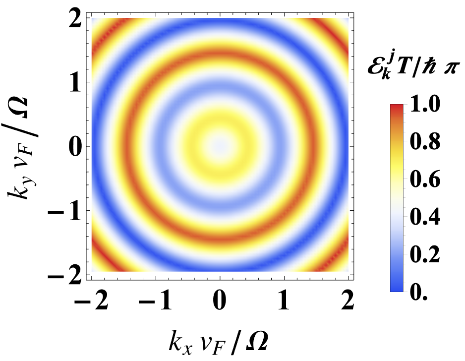
a) b)

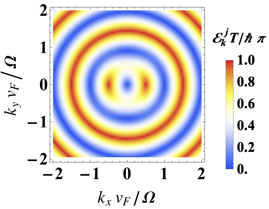
Figure 1: Quasi energy spectrum $\mathcal{E}_{\boldsymbol{k}}^{j}T/\hbar$ as a function of $k_{x}$ and $k_{y}$ for (a) circularly polarized light ($ev_{F}E_{x}/\hbar\Omega^{2}=0.5$, $ev_{F}E_{y}/\hbar\Omega^{2}=0.5$) and (b) linearly polarized light ($ev_{F}E_{x}/\hbar\Omega^{2}=0.5$, $ev_{F}E_{y}/\hbar\Omega^{2}=0.0$) in the weak electric fields regime.

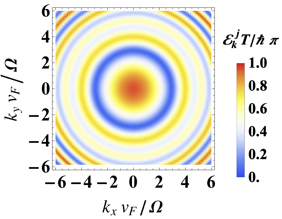
a) b)

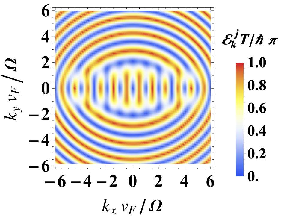
Figure 2: Quasi energy spectrum $\mathcal{E}_{\boldsymbol{k}}^{j}T/\hbar$ as a function of $k_{x}$ and $k_{y}$ for (a) circularly polarized light ($ev_{F}E_{x}/\hbar\Omega^{2}=ev_{F}E_{y}/\hbar\Omega^{2}=5.0$) and (b) linearly polarized light ($ev_{F}E_{x}/\hbar\Omega^{2}=5.0$, $ev_{F}E_{y}/\hbar\Omega^{2}=0.0$) in the strong electric field regime.

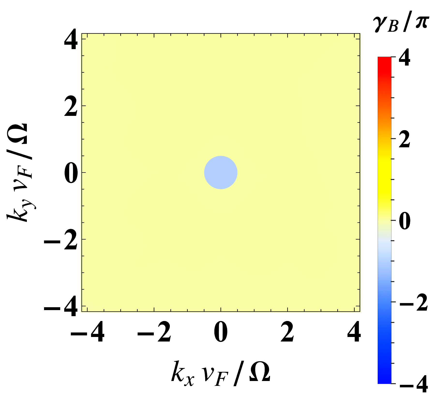
a) b)

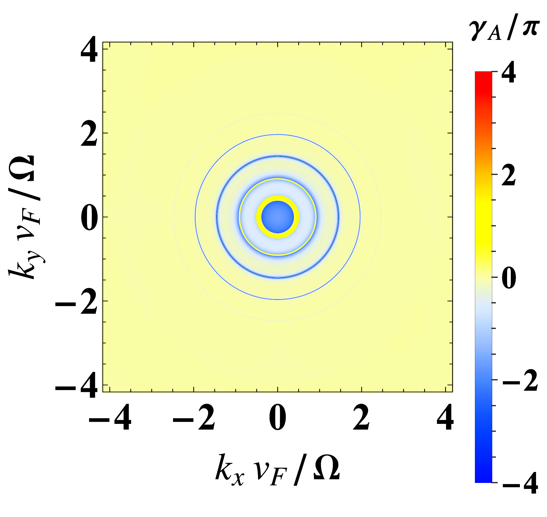
Figure 3: Topological phases for circular polarized light in the weak electric fields regime ($ev_{F}E_{x}/\hbar\Omega^{2}=ev_{F}E_{y}/\hbar\Omega^{2}=0.5$). Panel a) presents the Berry phase as obtained from the Dirac-Bloch formalism. Panel b) presents the Aharonov-Anandan phase obtained from solving Eq. (26). The Berry phase is non-trivial, $\gamma_{B,\boldsymbol{k}}=-\pi$, only within a circular light blue region centered at the Dirac point, with a radius determined by the magnitude of the electric field, while it remains trivial in the light yellow region. In contrast, the Aharonov-Anandan phase exhibits the same circular region but also features concentric rings, indicating multiphoton transitions.

III Berry and Aharonov-Anandan phases in time-driven graphene

To analyze this problem in detail, we consider the external driving of the graphene's effective Hamiltonian by an electromagnetic wave with angular frequency $\Omega$, propagating along the $z$-direction, perpendicular to the 2D lattice plane and described by a vector potential $\boldsymbol{A}(t)$ [16, 34, 27, 35, 36].

Here we study four different cases: linearly polarized light in the weak and strong field regimes and elliptically polarized light in the weak and strong field regimes. We assume that for those cases in which light is linearly polarized the vector potential takes the form:

$$\boldsymbol{A}(t)=\left(\frac{E_{x}}{\Omega}\cos{(\Omega t)},0\right),$$ (27)

where $E_{x}$ is the amplitude of the electric field. In those where the light excitation is elliptically polarized the vector potential is given by:

$$\boldsymbol{A}(t)=\left(\frac{E_{x}}{\Omega}\cos{(\Omega t)},\frac{E_{y}}{\Omega}\sin{(\Omega t)}\right),$$ (28)

where $E_{y}$ represents the amplitude of the electric field in the $y$-direction.

As explained in Appendix A, the time dependent equation given by Eq. (5) contains an adimensional parameter,

$$q_{0}=ev_{F}\sqrt{E_{x}^{2}+E_{y}^{2}}/\hbar\Omega^{2}$$ (29)

that defines the limits between weak ($q_{0}<1$) and strong ($q_{0}>1$) external driving fields. Finally, to compare the two different topological phases, we numerically solved Eq. (4) using the two approaches: Dirac-Bloch and Floquet. Below we outline the details of such calculations.

III.1 Berry phase

To calculate the Berry phase, we consider the Dirac- Bloch formalism [37, 38, 39, 35, 28, 27, 40, 34, 17, 16, 30, 41, 42] using the following ansatz,

$$\Psi_{\boldsymbol{k}}(t)=\sum_{\lambda}c^{\lambda}_{\boldsymbol{k}}(t)\varphi^{\lambda}_{\boldsymbol{k}}(t)\mathrm{e}^{-i\gamma^{\lambda}_{D,\boldsymbol{k}}(t)},$$ (30)

The instantaneous eigenvalues and eigenvectors were found from

$$\hbar v_{F}\boldsymbol{\sigma}_{\xi}\cdot\left[\boldsymbol{k}+\frac{e}{\hbar}\boldsymbol{A}(t)\right]\varphi^{\lambda}_{\boldsymbol{k}}(t)=\epsilon^{\lambda}_{\boldsymbol{k}}(t)\varphi^{\lambda}_{\boldsymbol{k}}(t).$$ (31)

where we have used the Hamiltonian given by Eq. (5).

The obtained eigenvalues and eigenvectors are then substituted into Eq. (13) to compute the Berry phase. Figure 3 a) shows the resulting Berry phase in reciprocal space for the weak electric field regime using circular polarization, while Fig. 4 a) presents the results for the strong electric field regime. The cases with linear polarization are not shown, as they yield trivial Berry phases. A discussion of these results is provided in Sec. IV.

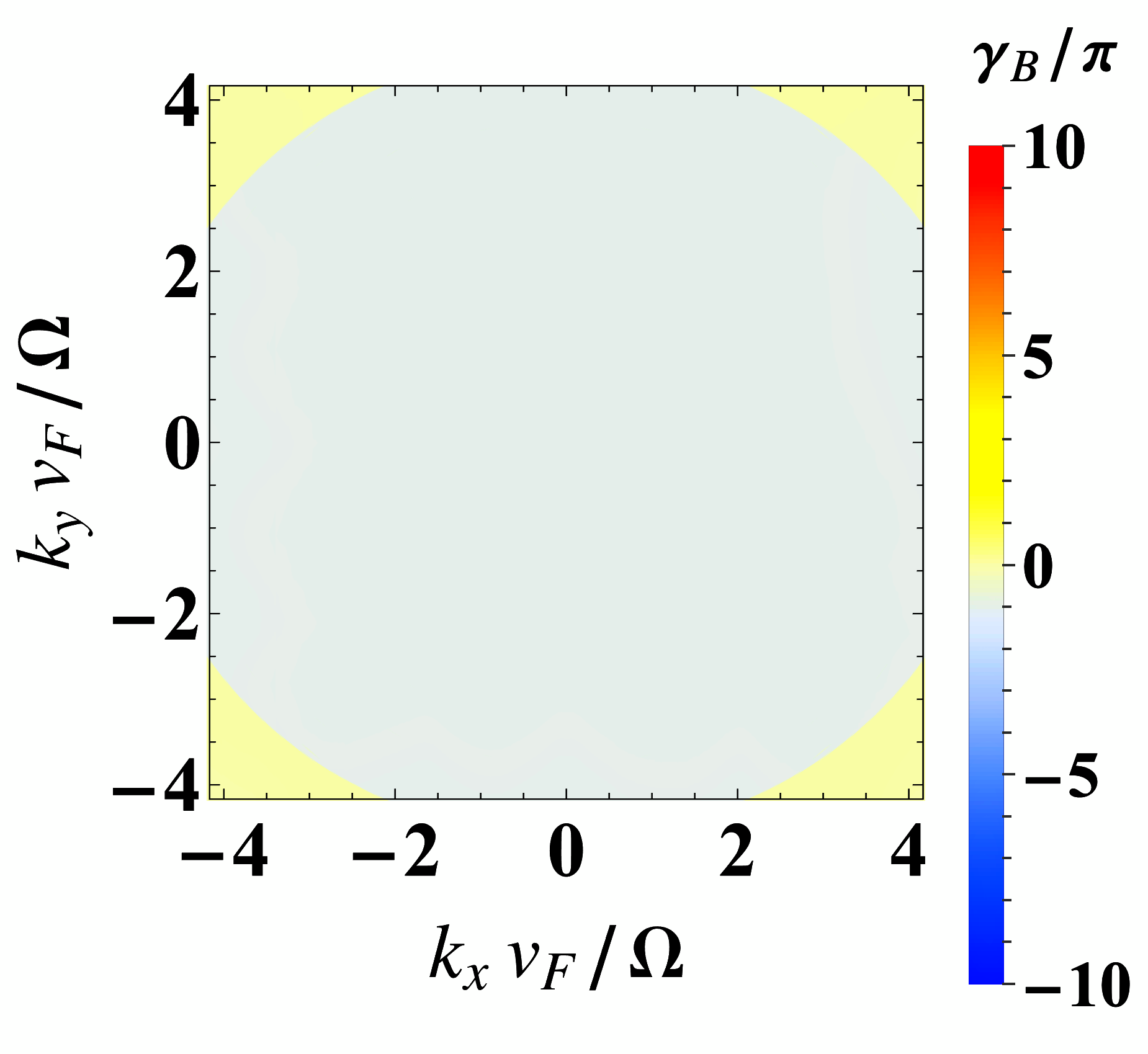
a) b)

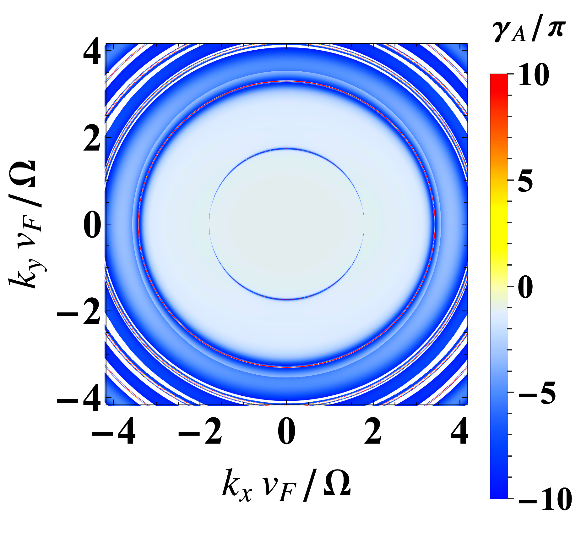
Figure 4: Topological phases for circular polarized light in the strong electric fields regime ($ev_{F}E_{x}/\hbar\Omega^{2}=5.0$, $ev_{F}E_{y}/\hbar\Omega^{2}=5.0$). a) Berry phase, b) Aharonov-Anandan phases. As in Fig. 3, the Berry phase is non-trivial $\gamma_{B,\boldsymbol{k}}=-\pi$, only within a circular light blue region centered at the Dirac point, with a radius determined by the magnitude of the electric field. The Aharonov-Anandan phase exhibits the same circular region but also features concentric rings, indicating multiphoton transitions.

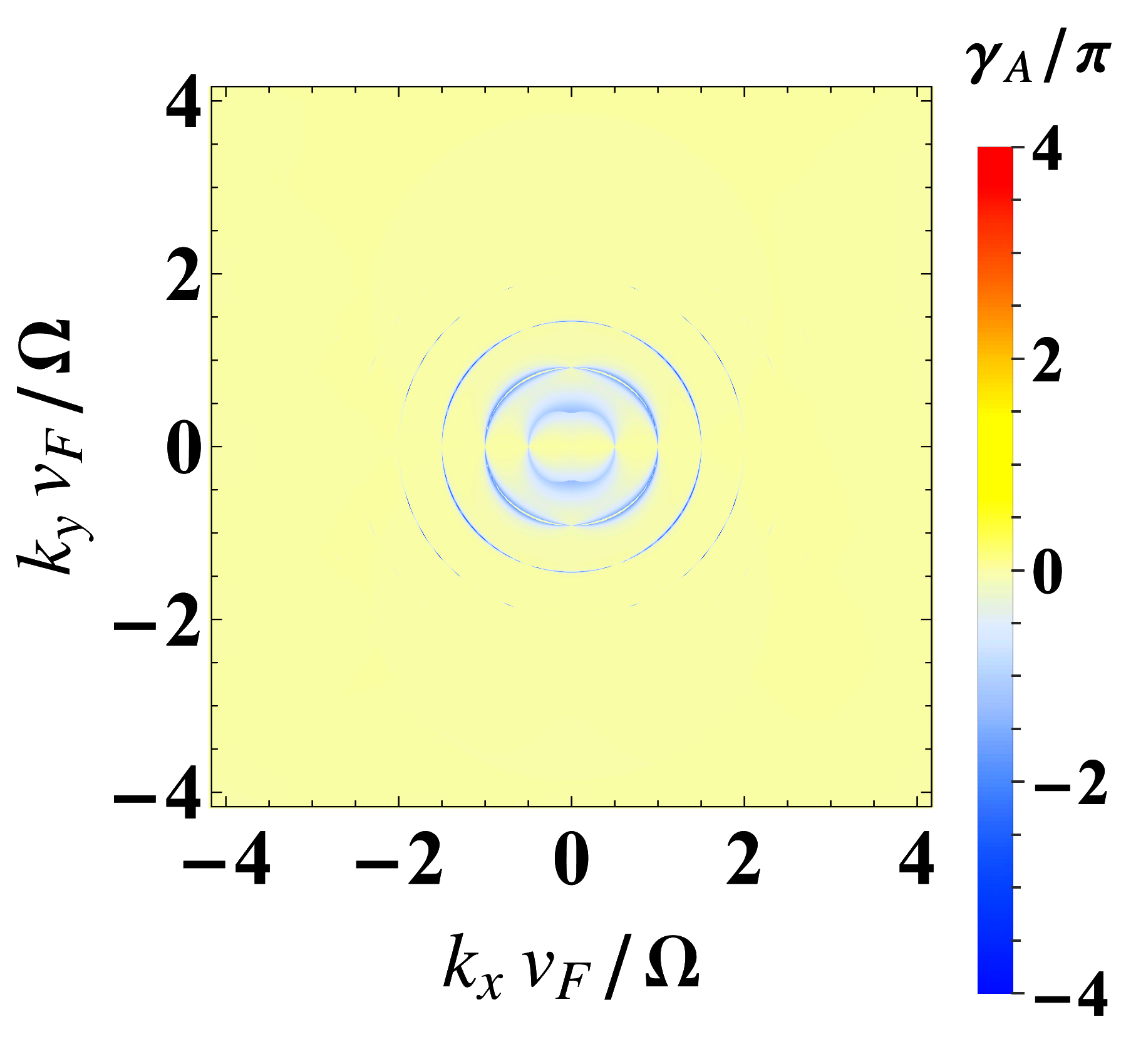
Figure 5: Topological Aharonov-Anandan phases for linear polarized light in the weak electric fields regime ($ev_{F}E_{x}/\hbar\Omega^{2}=0.5$, $ev_{F}E_{y}/\hbar\Omega^{2}=0.0$). The phase vanishes for momenta in the light yellow region, particularly for those parallel to the applied field ($k_{y}=0$). Note that for this case of linear polarization, the Berry phase is always zero throughout the entire reciprocal space; therefore, we do not include such a trivial plot.

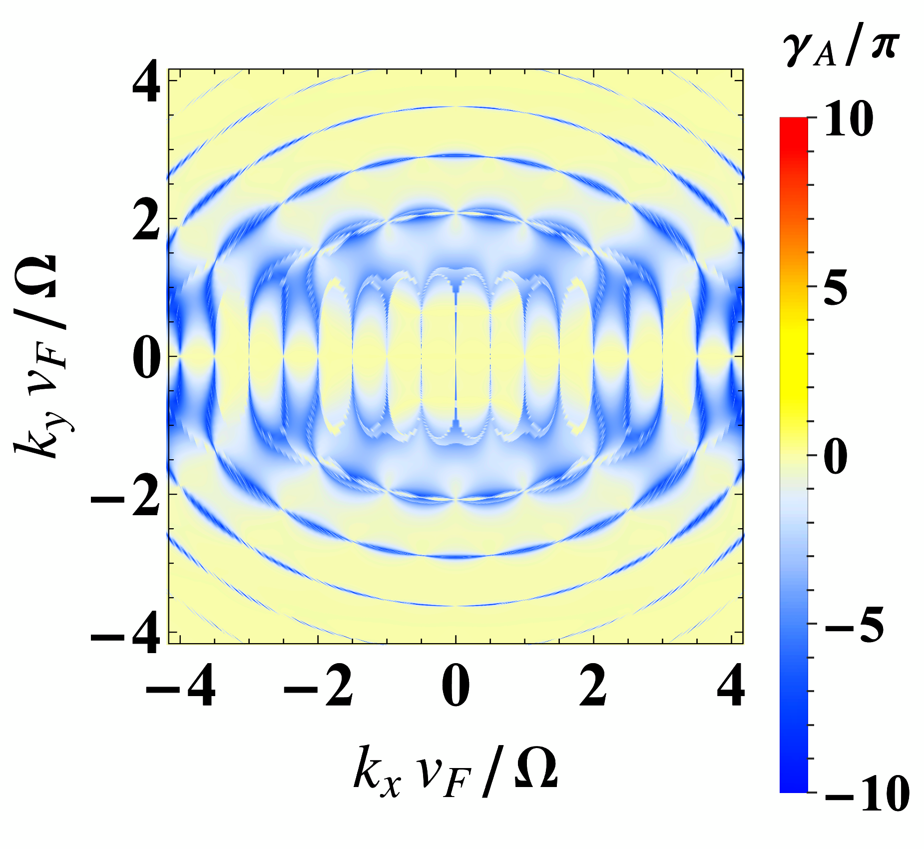
Figure 6: Topological Aharonov-Anandan phases for linearly polarized light in the strong electric field regime ($q_{0}=ev_{F}E_{x}/\hbar\Omega^{2}=5.0$, $ev_{F}E_{y}/\hbar\Omega^{2}=0.0$). As in the weak field regime, the phase vanishes for momenta parallel to the applied field ($k_{y}=0$), the phase vanishes. Under these same conditions, the Berry phase is zero throughout the entire reciprocal space and is therefore not shown.

III.2 Aharonov-Anandan phase

To find the Aharonov-Anandan phase, we numerically solve the Schrödinger equation (17) considering the Hamiltonian in Eq. (5). The wave function was obtained using Floquet theory via Eq. (20), as detailed in Refs. [43, 22]. The dynamical phase, $\gamma_{D,\boldsymbol{k}}$, can be determined by first computing $\mathcal{E}_{\boldsymbol{k}}^{j}T/\hbar$, which corresponds to the argument of the eigenvalues of the evolution operator, given by $U_{\boldsymbol{k}}(T)=\exp(-i/\hbar\hat{H}_{e,\boldsymbol{k}}T)$. Obtaining the corresponding eigenvectors, we use Eq. (26) to calculate the Aharonov-Anandan phase. Finally, from Eq. (23), we derive the dynamical phase, $\gamma_{\boldsymbol{k}}^{j}(T)$.

Figure 1 displays the positive quasienergy, $\mathcal{E}_{\boldsymbol{k}}^{1}T/\hbar$ ($j=1$), of the Floquet state $\boldsymbol{\Psi}_{\boldsymbol{k}}^{1}(t)$ as a function of $k_{x}$ and $k_{y}$ for (a) circularly and (b) linearly polarized light in the weak-field regime. In both cases the spectrum is distorted compared to the free electron case from the Dirac point outwards up to $v_{F}(k_{x}^{2}+k_{y}^{2})^{1/2}/\Omega\approx 0.5$. Beyond this line the free-electron spectrum is recovered. Under circularly polarized light, the quasi-energy spectrum exhibits circular symmetry, whereas under linearly polarized excitation, it is slightly stretched along the $k_{x}$ axis. Additionally, the circularly polarized excitation induces a gap at the Dirac point, while in the linear case, the Dirac point remains gapless

In Fig. 2 we observe the behavior of the positive quasienergy $\mathcal{E}_{\boldsymbol{k}}^{1}T/\hbar$ as a function of $k_{x}$ and $k_{y}$ for (a) circularly and (b) linearly polarized light in the strong field regime. In both cases the spectrum is distorted in comparison with the free electron case from the Dirac point outwards up to $v_{F}(k_{x}^{2}+k_{y}^{2})^{1/2}/\Omega\approx 5.0$. As in the low field regime, beyond this line the free-electron spectrum is recovered. The distortions are however much larger than in the weak-field regime. Under the circularly polarized light the quasi spectrum newly has circular symmetry. The linearly polarized excitation is strongly stretched along the $k_{x}$ axis and vertical lines appear along $k_{y}$. Additionally, under circularly polarized light the gap that opens up close to the Dirac point is much larger than in the weak-field regime. In the linear case the Dirac point remains.

The shape of the quasispectrum in Figs. 1 and 2 is in fact determined by an effective Whittaker and Hill diferential equation with complex parameters, see Appendix A.

Finally, once the Floquet states are found using Eq. (20), the Aharonov-Anandan phase is calculated through Eq. (26). Figs. 3,4,5 and 6 present the resulting Aharonov-Anandan phases in reciprocal space for the weak and strong-field regimes using different polarizations. The discussion of these results is given in Sec. IV.

IV Discussion and remarks

Let us discuss the main features observed in the numerically obtained plots.

IV.1 Weak external field

In Figs. 3 we present the Berry and Aharonov-Anandan phases in the weak-field regime using circular polarized light. The Berry phase is different from zero, $\gamma_{B,\boldsymbol{k}}=-\pi$, in a region centered at the tip of the Dirac cone, as seen in Fig. 3 a) as a light blue circle. This justifies the idea of assigning a topological charge to the Dirac cone [44], even if the adiabatic condition is never met at the cone tip. The radius of the non trivial topological Berry phase is determined by the magnitude of the electric field, while it remains trivial in the light yellow region. Meanwhile, as seen in Figs. 3 b), the Aharonov-Anandan phase is also different from zero in the same region but also presents several concentric rings. As we shall discuss later, such rings are associated with transitions from the valence band to the conduction band. The Aharonov-Anandan phase in Fig. 4 b) exhibits a similar behavior. However, in this case there are strong distortions within the circle of radius $q_{0}=ev_{F}E/\hbar\Omega$. Outside this circle the typical thin lines corresponding to the resonance condition reappear as in the weak-field case.

In Fig. 5, we present the case of linearly polarized light. The Berry phase is not included, as it remains trivial for all values of $\boldsymbol{k}$. Instead, the Aharonov-Anandan phase exhibits a much richer and more intricate structure. For instance, along the $k_{x}$-axis ($k_{y}=0$), the Aharonov-Anandan phase is zero, a fact that will be explained later. Additionally, the rings observed in Fig. 3 are now deformed, transforming into ellipses that eventually recover their circular shape.

IV.2 Strong external field

Fig. 4 presents the Berry and Aharonov-Anandan phases for the strong external field case with circular polarization. Its structure is similar to the case of a weak-field except that the radius is expanded due to the bigger magnitude of the electric field. Again the Berry phase is non-trivial only within a circle around the Dirac cone. In contrast, the Aharonov-Anandan phase seen in Fig. 4 b) exhibits concentric rings, indicating multiphoton transitions.

The Aharonov-Anandan phases shown in Fig. 6 exhibit a rather intriguing behavior. First the phase is zero along the $k_{y}=0$, meaning that for states with momentum only in the direction of the applied field, the phase remains zero. For states with $k_{y}\neq 0$, the rings observed in Fig. 4b) transform into ellipses with a modulation that creates a pearl-necklace-like structure. In this case, the Berry phase does not provide information about these structures, as it remains zero throughout the reciprocal space.

IV.3 Remarks on the phases

In summary, for linearly polarized light, the Berry phase yields trivial results. In contrast, for circularly polarized light, the Berry phase is nonzero only in a region around the Dirac cone where the adiabatic condition is not met. This region, determined in reciprocal space by the strength and frequency of the external drive, also exhibits a nonzero Aharonov-Anandan phase. However, the Aharonov-Anandan phase reveals much more structure, which can be understood by considering band transitions..

It can be shown from Eq. (10) and the Stokes theorem that the Berry phase in Eq. (12) can be rewritten as:

$$\gamma_{B,\boldsymbol{k}}^{\lambda}=\frac{1}{2}\oint_{C}\frac{K_{y}(t)dK_{x}(t)-K_{x}(t)dK_{y}(t)}{K_{x}^{2}(t)+K_{y}^{2}(t)}\\ =-\frac{1}{2}\int_{S}dK_{x}dK_{y}\bigg{[}\frac{\partial}{\partial K_{x}}\left(\frac{K_{y}}{K_{x}^{2}+K_{y}^{2}}\right)\\ +\frac{\partial}{\partial K_{y}}\left(\frac{K_{x}}{K_{x}^{2}+K_{y}^{2}}\right)\bigg{]},$$ (32)

where $K_{x}(t)$ and $K_{y}(t)$ are the components of $\boldsymbol{K}(t)$. Here, $C$ is the contour traced by the vector potential over one period $T$, and $S$ is the surface enclosed by this contour.

This integral evaluates to $-\pi$ as long as the singularity at $\boldsymbol{k}=\boldsymbol{0}$ lies inside the contour $C$. Conversely, if the singularity lies outside the contour $C$, the right-hand side of Eq. (32) vanishes trivially. In the specific case where the vector potential is given by Eq. (28), the Berry phase is $-\pi$ if the ellipse centered at $(k_{x},k_{y})$, with semi-minor and semi-major axes equal to $eE_{x}/\hbar\Omega$ and $eE_{y}/\hbar\Omega$, respectively, contains the origin in reciprocal space. Otherwise, the Berry phase vanishes. In this way, when graphene is subject to linearly polarized light ($E_{x}\neq 0$ and $E_{y}=0$) the eccentricity of the ellipse is zero and the Berry phase vanishes all over the reciprocal space. Instead, under circularly polarized light the eccentricity of the ellipse is one. This is confirmed in the numerical simulations; we observe in Figs. 3 a) and 4 a) that the Berry phase is $-\pi$ inside the circle of radius $eE_{x}/\hbar\Omega=eE_{y}/\hbar\Omega$ and $0$ elsewhere.

Regarding the Aharonov-Anandan phase we note the following points:

1. The rings that form in the Aharonov-Anandan phase in the weak field regime under circularly polarized excitation shown in Fig. 3 are consistent with the resonance condition $2\epsilon_{\boldsymbol{k}}=2q\hbar\omega$ for $q=1,2,\dots$ photons as it was shown in the rotating wave approximation [43].

2. The Aharonov-Anandan phase also presents rings in the weak field regime but under linearly polarized light, as can be seen in Fig. 5. However, in this case the rings disappear near the region where $k_{y}=0$ where the transitions between the valence and conduction bands are forbidden as we demonstrate below. When $ky=0$ and under linearly polarized light ($E_{y}=0$) the evolution operator is obtained from the Hamiltonian in Eq. (5) giving

   $$U(t)=\exp\left[-iv_{F}\alpha(t)\sigma_{x}\right],$$ (33)

   where

   $$\alpha(t)=k_{x}t+\frac{eE_{x}}{\hbar\Omega^{2}}\sin(\Omega t).$$ (34)

   Under this very particular set of conditions, the conduction and valence band states

   $$\psi_{C}=\frac{1}{\sqrt{2}}\left(\begin{array}[]{c}1\\ 1\end{array}\right),\,\,\,\,\,\,\psi_{V}=\frac{1}{\sqrt{2}}\left(\begin{array}[]{c}1\\ -1\end{array}\right),$$ (35)

   also correspond to the Floquet states with quasi energies $\mathcal{E}^{\pm 1}=\pm\hbar v_{F}k_{x}$. The transition probabilities between these two states vanish, namely

   $$\left\langle\psi_{C}\left|U(t)\right|\psi_{V}\right\rangle=0$$ (36)

   Moreover, assuming that the system begins in the conduction band, the time dependent wave function is given by

   $$\psi(t)=\frac{1}{\sqrt{2}}\left(\begin{array}[]{c}\mathrm{e}^{i\alpha(t)}\\ -\mathrm{e}^{i\alpha(t)}\end{array}\right)$$ (37)

   The Andandan phase of Eq. (26) in this case vanishes because $w_{\boldsymbol{k}}^{j}=1$ for any of the bands and therefore $dw_{\boldsymbol{k}}^{j}=0$. This can be clearly seen in Figs. 5 and 6 where $\gamma_{A,\boldsymbol{k}}^{j}=0$ in the $k_{x}$-direction where $k_{y}=0$. A similar argument can be made in the bipartite lattice base

   $$\psi_{A}=\left(\begin{array}[]{c}1\\ 0\end{array}\right),\,\,\,\,\,\,\psi_{B}=\left(\begin{array}[]{c}0\\ 1\end{array}\right),$$ (38)

   where the Aharonov-Anandan phase is given by $\gamma_{A,\boldsymbol{k}}=-\int_{0}^{T}\tan{\alpha(t)}d\alpha(t)/dtdt=0$.

   An alternative approach is shown in Appendix A, as is possible to derive the trivial nature of the phases for $k_{y}=0$ from integrating a Whittaker-Hill equation.

3. This also explains some other features of the Aharonov-Anandan phase in the strong field regime observed in Fig. 6 as the vertical lines with values of $\gamma_{A,\boldsymbol{k}}\neq 0$ in the vicinity of $-\pi$ in the region of reciprocal space where the field dominates ($k<eE_{x}/\hbar\Omega$). In this region the symmetry in reciprocal space is strongly broken by the field producing vertical lines. As we move far from this region ($k>eE_{x}/\hbar\Omega$) the symmetry is restored and the transition lines that comply with the resonance condition $2\epsilon_{\boldsymbol{k}}=2q\hbar\omega$ recover the circular symmetry. However, the distortions of the oscillating electric field along the $k_{x}$-direction are still observed as small modulations in the transition lines.

4. Thus in general, it can be established that $\gamma_{A,\boldsymbol{k}}\neq 0$ ($\approx-\pi$) where the resonance condition is met ($2\epsilon(\boldsymbol{k})=q\hbar\omega$ where $q=1,2\dots,n$) and $\gamma_{A,\boldsymbol{k}}=0$ between the transition lines. It is then natural to ask ourselves why is there a connection between the transitions and the Aharonov-Anandan phase. This question can be answered through the following argument. Weather in the conduction-valence band basis $\psi_{V}$, $\psi_{C}$ or the bipartite lattice basis $\psi_{A}$, $\psi_{B}$ the Floquet wave function must be of the form

   $$\psi^{j}_{\boldsymbol{k}}(t)=\exp\left(-i\frac{\mathcal{E}^{j}_{\boldsymbol{k}}}{\hbar}t\right)\mathrm{e}^{i\chi(t)}\left(\begin{array}[]{c}\mathrm{e}^{i\beta(t)}a(t)\\ b(t)\end{array}\right)$$ (39)

   where, in accordance with the Floquet theorem, $\mathcal{E}^{j}_{\boldsymbol{k}}$ is the quasi energy, and $\chi(t)$, $\beta(t)$, $a(t)$ and $b(t)$ real numbers and are periodic with period $T$. The Aharonov-Anandan phase that arises from this wave function is

   $$\gamma_{A,\boldsymbol{k}}=\frac{1}{2}\int_{0}^{T}\dot{\beta}(t)\frac{a^{2}(t)}{a^{2}(t)+b^{2}(t)}dt.$$ (40)

   Far away from the resonant condition $a(t)$ and $b(t)$ are constants. In this case the Aharonov-Anandan phase is

   $$\gamma_{A,\boldsymbol{k}}=\frac{1}{2}\frac{a^{2}(t)}{a^{2}(t)+b^{2}(t)}\int_{0}^{T}\dot{\beta}(t)dt=0.$$ (41)

   If, on the contrary, the resonant condition is met, $a(t)$ and $b(t)$ are time dependent and and the behaviour of the Anandan phase is non-trivial.

   In Fig. 7, we have used the difference between the maximum and minimum probabilities of the Floquet state being in site $A$ ($\psi_{A}$) during a period $T$ as a measure of the transition probability. Similar results are obtained by subtracting the minimum and maximum probabilities of being in the conduction band, though they are not shown here. Given the strong resemblance between these density plots and the Aharonov-Anandan phase, along with the result of Eq. (41), it is evident that $\gamma_{A,\boldsymbol{k}}$ encodes information about the transitions induced by the periodic drive.

5. The connection between the Berry and Aharonov-Anandan phases can also be worked out from a perturbative approach of the time-evolution operator as shown in Appendix B.

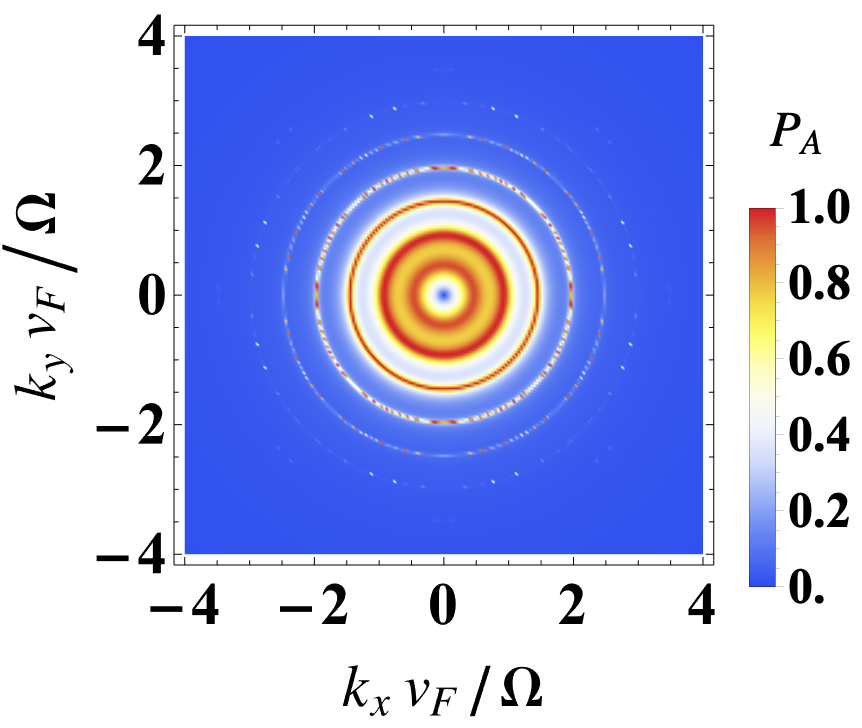
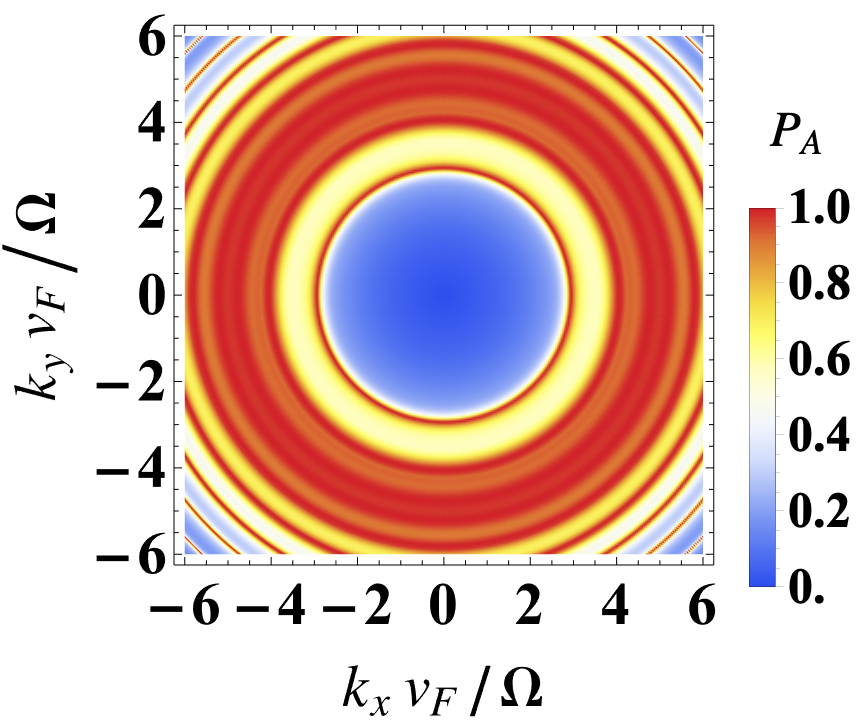
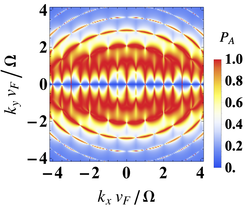
Figure 7: Transition probability as a function of $k_{x}v_{f}/\Omega$ and $k_{y}v_{f}/\Omega$ for (a) circularly polarized light in the weak electric field regime ($q_{0}=ev_{F}E_{x}/\hbar\Omega^{2}=0.5$, $ev_{F}E_{y}/\hbar\Omega^{2}=0.5$) and (b) circularly polarized light in the strong electric field regime ($q_{0}=ev_{F}E_{x}/\hbar\Omega^{2}=5.0$, $ev_{F}E_{y}/\hbar\Omega^{2}=5.0$), (c) linearly polarized light in the weak electric field regime ($q_{0}=ev_{F}E_{x}/\hbar\Omega^{2}=0.5$, $ev_{F}E_{y}/\hbar\Omega^{2}=0.0$), (d) linearly polarized light in the strong electric field regime ($q_{0}=ev_{F}E_{x}/\hbar\Omega^{2}=5.0$, $ev_{F}E_{y}/\hbar\Omega^{2}=0.0$).

V Conclusions

Although many solid-state systems are gapless, the Berry topological phase is derived from a trajectory in parameter space without accounting for the breakdown of the adiabatic approximation. While the Berry phase can always be computed using well-known formulae, it does not provide insight into the limits of adiabaticity. Determining these limits requires a time-dependent approach, as demonstrated here for graphene under electromagnetic radiation. We also show that the Aharonov-Anandan phase serves as a valuable alternative for weak fields, as it coincides with the Berry phase while offering additional insights, such as identifying regions of multiphoton transitions.

The Berry and dynamical phases derived from the Dirac-Bloch formalism are solely determined by the contour of the vector potential. Consequently, these topological phases can be engineered by simply adjusting the polarization state and overall shape of the incident light. In contrast, tailoring the Aharonov-Anandan phase and its associated dynamical phases, which emerge from the Floquet formalism, is more challenging, as their evolution is entirely governed by the time-dependent dynamics of the wave function.

In stark contrast with the Berry phase, that represents the phase acquired by the wave function remaining in the same sate, the Aharonov-Anandan phase encodes information of the transition between levels.

Appendix A Quasienergy spectrum of graphene under time dependent radiation.

In this section, we study the time-dependent Eq. (1), focusing on the most interesting result observed in the numerical simulations: the case of linear polarization. The evolution of the wave function is given by solving Eq. 1. The solution can be found by using the Floquet theory. This requires to uncouple the spinor components in the Dirac time-dependent equation. Consider the linear polarized case given by Eq. (27). First we apply a rotation around the $y$ axis [22],

$$\mathbf{\Psi}(t)=\exp\left[-i\left(\frac{\pi}{4}\right)\hat{\sigma}_{y}\right]\mathbf{\Phi}(t).$$ (42)

Substituting (42) into Eq. (1) we obtain,

$$i\frac{d}{d\phi}\mathbf{\Phi}(\phi)=\frac{2}{\hbar\Omega}\left[\tilde{\Pi}_{x}\hat{\sigma}_{z}+\tilde{k}_{y}\hat{\sigma}_{y}\right]\mathbf{\mathbf{\Phi}}(\phi)\,,$$ (43)

where we defined $\tilde{k}_{x}=\hbar v_{F}k_{x},\tilde{k}_{y}=\hbar v_{F}k_{y}$ In what follows, we will use a scaled time $\phi=\Omega t/2$, a scaled momentum $\tilde{\Pi}_{x}=\tilde{k}_{x}-\zeta_{x}\cos(2\phi)$ and a frequency-weighted induced dipole moment,

$$\zeta_{x}=\frac{ev_{x}E_{x}}{\Omega}.$$ (44)

The spinor components of $\mathbf{\Phi}(\phi)=\left(\Phi_{+}(\phi),\Phi_{-}(\phi)\right)^{\top}$ are given by $\Phi_{+}(\phi)=[\Psi_{A}(\phi)+\Psi_{B}(\phi)]/\sqrt{2}$ and $\Phi_{-}(\phi)=[\Psi_{A}(\phi)-\Psi_{B}(\phi)]/\sqrt{2}$. A final tranformation allows to remove the term proportional to $\hat{\sigma}_{0}$ in Eq. (43)

$$\mathbf{\Phi}(\phi)=\exp\left[-2i\frac{\tilde{k}_{y}}{\hbar\Omega}\,\phi\,\hat{\sigma}_{0}\right]\mathbf{\chi}(\phi),$$ (45)

where $\mathbf{\chi}(\phi)=(\chi_{+1}(\phi),\chi_{-1}(\phi))^{\top}$. Finally, if Eq. (45) is inserted into Eq. (43), the following Whittaker-Hill differential equation is found,

$$\chi_{\eta}^{\prime\prime}(\phi)+4\bigg{[}\left(\frac{\tilde{k}_{x}}{\hbar\Omega}-q_{0}\cos(2\phi)\right)^{2}+\left(\frac{\tilde{k}_{y}}{\hbar\Omega}\right)^{2}\\ +i\eta q_{0}\sin(2\phi)\bigg{]}\chi_{\eta}(\phi)=0.$$ (46)

where $\eta=1,2$ is a label for the spinor component and $q_{0}$ is an important parameter that defines the cases of weak ($q_{0}>1$) and intense fields ($q_{0}<1$),

$$q_{0}=\frac{\zeta_{x}}{\hbar\Omega}=\frac{ev_{F}E_{x}}{\hbar\Omega^{2}}$$ (47)

For the circular polarized case, a similar calculation replaces $E_{x}$ by the norm of the electric field. Notice that the transition region $q_{0}=1$ is clearly seen in Fig. 2 b). We remark that in Eq. (46) the spinors components are completely decoupled. A further advantage is that $\chi_{+1}(\phi)$ and $\chi_{-1}(\phi)$ are the probability amplitudes of the valence and conduction band, respectively.

The case $k_{y}=0$ can always be integrated for any field intensity,

$$\chi_{\eta}(t)=\chi_{\eta}(0)\exp\left[i\eta\left(q_{0}\sin{(\Omega t)}-\frac{\epsilon_{\boldsymbol{k}}t}{\hbar}\right)\right].$$ (48)

with $\epsilon_{\boldsymbol{k}}=\sqrt{\tilde{k}_{x}^{2}+\tilde{k}_{y}^{2}}$. From here if follows that the Berry and Aharonov phases are always zero in agreement with Figs. 4 and 6. The transitions between states are seen in Eq. (46) by considering gaps in the stability chart diagram of the Whittaker and Hill equation with complex parameters [45, 46].

Appendix B Topological phases obtained from the time-evolution operator

To establish the relationship between the Aharonov-Anandan phase, $\gamma_{A,\boldsymbol{k}}$, and the Berry phase, $\gamma_{B,\boldsymbol{k}}$, we rewrite the Hamiltonian from Eq. (5) for $\xi=1$, in terms of the eigenenergies and instantaneous phases as,

$$\hat{\mathcal{H}}_{\boldsymbol{k}}=|\epsilon_{\boldsymbol{k}}^{\lambda}(t)|\begin{pmatrix}0&e^{-i\theta_{\boldsymbol{k}}(t)}\\ e^{i\theta_{\boldsymbol{k}}(t)}&0\end{pmatrix}.$$ (49)

Next, we define the unitary rotation transformation:

$$\begin{split}\mathcal{R}(t)&\equiv\frac{1}{\sqrt{2}}\begin{pmatrix}1&1\\ -e^{i\theta_{\boldsymbol{k}}(t)}&e^{i\theta_{\boldsymbol{k}}(t)}\end{pmatrix},\\ \mathcal{R}^{\dagger}(t)&\equiv\frac{1}{\sqrt{2}}\begin{pmatrix}1&-e^{-i\theta_{\boldsymbol{k}}(t)}\\ 1&e^{-i\theta_{\boldsymbol{k}}(t)}\end{pmatrix}.\end{split}$$ (50)

This allows us to rewrite the Schrödinger equation in the transformed state as:

$$i\hbar\frac{d}{dt}\varphi_{\boldsymbol{k}}(t)=\overline{\mathcal{H}}_{\boldsymbol{k}}\varphi_{\boldsymbol{k}}(t)$$ (51)

Here, the transformed state $\varphi_{\boldsymbol{k}}(t)$ and the effective Hamiltonian $\overline{\mathcal{H}}_{\boldsymbol{k}}$ are defined as:

$$\begin{split}\varphi_{\boldsymbol{k}}(t)&\equiv\mathcal{R}^{\dagger}(t)\psi_{\boldsymbol{k}}(t)\\ \overline{\mathcal{H}}_{\boldsymbol{k}}(t)&\equiv\left\{\mathcal{R}^{\dagger}(t)\hat{\mathcal{H}}_{\boldsymbol{k}}\mathcal{R}(t)-i\hbar\mathcal{R}^{\dagger}(t)\frac{d}{dt}\mathcal{R}(t)\right\}\\ &=-\left\{|\epsilon_{\boldsymbol{k}}^{\lambda}(t)|+\hbar\frac{d\gamma_{B,\boldsymbol{k}}(t)}{dt}\sigma_{0}+\hbar\nu_{\boldsymbol{k}}(t)\sigma_{x}\right\}\end{split}$$ (52)

It can be seen that, with the basis transformation, the Hamiltonian is rewritten in terms of the time derivative of the dynamic, Berry, and Rabi phases.

The unitary time evolution operator can be approximated as:

$$\begin{split}\hat{\mathcal{U}}(t)&=\exp\left\{-\frac{i}{\hbar}\int_{0}^{t}\overline{\mathcal{H}}_{\boldsymbol{k}}(t^{\prime})dt^{\prime}\right.\\ &\left.-\frac{1}{\hbar^{2}}\int_{0}^{t}dt^{\prime}\int_{0}^{t^{\prime}}dt^{\prime\prime}\left[\overline{\mathcal{H}}_{\boldsymbol{k}}(t^{\prime}),\overline{\mathcal{H}}_{\boldsymbol{k}}(t^{\prime\prime})\right]\right.\\ &\left.+\frac{i}{\hbar^{3}}\int_{0}^{t}dt^{\prime}\int_{0}^{t^{\prime}}dt^{\prime\prime}\int_{0}^{t^{\prime\prime}}dt^{\prime\prime\prime}\left[\overline{\mathcal{H}}_{\boldsymbol{k}}(t^{\prime}),\left[\overline{\mathcal{H}}_{\boldsymbol{k}}(t^{\prime\prime}),\overline{\mathcal{H}}_{\boldsymbol{k}}(t^{\prime\prime\prime})\right]\right]+\ldots\right\}\end{split}$$ (53)

By evaluating the integrals term by term, we obtain the following contributions:

$$\begin{split}-\frac{i}{\hbar}\int_{0}^{t}\overline{\mathcal{H}}_{\boldsymbol{k}}(t^{\prime})dt^{\prime}&=i\left(|\gamma^{\lambda}_{D,\boldsymbol{k}}(t)|\sigma_{z}\right.\\ &\left.+\gamma_{B,\boldsymbol{k}}\sigma_{0}+\gamma_{R,\boldsymbol{k}}\sigma_{x}\right)\\ -\frac{1}{\hbar^{2}}\int_{0}^{t}dt^{\prime}\int_{0}^{t^{\prime}}dt^{\prime\prime}\left[\overline{\mathcal{H}}_{\boldsymbol{k}}(t^{\prime}),\overline{\mathcal{H}}_{\boldsymbol{k}}(t^{\prime\prime})\right]&=2i\\ &\times\left\{\int_{0}^{t}dt^{\prime}\nu_{\boldsymbol{k}}(t^{\prime})|\gamma^{\lambda}_{D,\boldsymbol{k}}(t^{\prime})|\right.\\ &\left.-\frac{1}{\hbar}\int_{0}^{t}dt^{\prime}|\epsilon_{\boldsymbol{k}}^{\lambda}(t^{\prime})|\gamma_{R,\boldsymbol{k}}(t^{\prime})\right\}\sigma_{y}\end{split}$$ (54)

For the next term we have:

$$\begin{split}\frac{i}{\hbar^{3}}\int_{0}^{t}dt^{\prime}\int_{0}^{t^{\prime}}dt^{\prime\prime}\int_{0}^{t^{\prime\prime}}dt^{\prime\prime\prime}\left[\overline{\mathcal{H}}_{\boldsymbol{k}}(t^{\prime}),\left[\overline{\mathcal{H}}_{\boldsymbol{k}}(t^{\prime\prime}),\overline{\mathcal{H}}_{\boldsymbol{k}}(t^{\prime\prime\prime})\right]\right]\\ =\frac{4i}{\hbar^{2}}\int_{0}^{t}\int_{0}^{t^{\prime}}\int_{0}^{t^{\prime\prime}}dt^{\prime}dt^{\prime\prime}dt^{\prime\prime\prime}\left[\hbar\nu_{\boldsymbol{k}}(t^{\prime})\sigma_{z}-|\epsilon^{\lambda}_{\boldsymbol{k}}(t^{\prime})|\sigma_{x}\right]\\ \times\left[\nu_{\boldsymbol{k}}(t^{\prime\prime})|\epsilon^{\lambda}_{\boldsymbol{k}}(t^{\prime\prime\prime})|-|\epsilon^{\lambda}_{\boldsymbol{k}}(t^{\prime\prime})|\nu_{\boldsymbol{k}}(t^{\prime\prime\prime})\right]\end{split}$$ (55)

Finally, the time evolution operator is:

$$\begin{split}\hat{\mathcal{U}}(t)&\approx\exp\left\{i\left(|\gamma^{\lambda}_{D,\boldsymbol{k}}(t)|\sigma_{z}+\gamma_{B,\boldsymbol{k}}(t)\sigma_{0}+\gamma_{R,\boldsymbol{k}}(t)\sigma_{x}\right)\right.\\ &+2i\left(\int_{0}^{t}dt^{\prime}\nu_{\boldsymbol{k}}(t^{\prime})|\gamma^{\lambda}_{D,\boldsymbol{k}}(t^{\prime})|-\frac{1}{\hbar}\int_{0}^{t}dt^{\prime}|\epsilon^{\lambda}_{\boldsymbol{k}}(t^{\prime})|\gamma_{R,\boldsymbol{k}}(t^{\prime})\right)\sigma_{y}\\ &+\frac{4i}{\hbar^{2}}\left(\int_{0}^{t}\int_{0}^{t^{\prime}}\int_{0}^{t^{\prime\prime}}dt^{\prime}dt^{\prime\prime}dt^{\prime\prime\prime}\left[\hbar\nu_{\boldsymbol{k}}(t^{\prime})\sigma_{z}-|\epsilon^{\lambda}_{\boldsymbol{k}}(t^{\prime})|\sigma_{x}\right]\right.\\ &\times\left.\left[\nu_{\boldsymbol{k}}(t^{\prime\prime})|\epsilon^{\lambda}_{\boldsymbol{k}}(t^{\prime\prime\prime})|-|\epsilon^{\lambda}_{\boldsymbol{k}}(t^{\prime\prime})|\nu_{\boldsymbol{k}}(t^{\prime\prime\prime})\right]\right\}\end{split}$$ (56)

It is important to note that in the adiabatic limit, with no transitions, the only phases present are the dynamic phase and the Berry phase, as expected. However, in the non-adiabatic case, correction terms related to transitions between energy levels emerge, particularly the Rabi phase term. These terms are generally incorporated into the Aharonov-Anandan geometric phase discussed in Sec. II.

References

- [1] B. Andrei Bernevig. Topological Insulators and Topological Superconductors. Princeton University Press, Princeton, 2013.
- [2] Liang Wu, M. Salehi, N. Koirala, J. Moon, S. Oh, and N. P. Armitage. Quantized faraday and kerr rotation and axion electrodynamics of a 3d topological insulator. Science, 354(6316):1124–1127, 2016.
- [3] J. W. McIver, B. Schulte, F.-U. Stein, T. Matsuyama, G. Jotzu, G. Meier, and A. Cavalleri. Light-induced anomalous hall effect in graphene. Nature Physics, 16(1):38–41, Jan 2020.
- [4] P. Phillips. Advanced Solid State Physics. Advanced Solid State Physics. Cambridge University Press, 2012.
- [5] Kai Wang, Steffen Weimann, Stefan Nolte, Armando Perez-Leija, and Alexander Szameit. Measuring the aharonov–anandan phase in multiport photonic systems. Opt. Lett., 41(8):1889–1892, Apr 2016.
- [6] Takashi Oka and Hideo Aoki. Photovoltaic hall effect in graphene. Phys. Rev. B, 79:081406, Feb 2009.
- [7] D. N. Basov, R. D. Averitt, and D. Hsieh. Towards properties on demand in quantum materials. Nature Materials, 16(11):1077–1088, Nov 2017.
- [8] D. J. Thouless, M. Kohmoto, M. P. Nightingale, and M. den Nijs. Quantized hall conductance in a two-dimensional periodic potential. Phys. Rev. Lett., 49:405–408, Aug 1982.
- [9] Eliahu Cohen, Hugo Larocque, Frédéric Bouchard, Farshad Nejadsattari, Yuval Gefen, and Ebrahim Karimi. Geometric phase from aharonov–bohm to pancharatnam–berry and beyond. Nature Reviews Physics, 1(7):437–449, 2019.
- [10] Xiaosong Zhu, Peixiang Lu, and Manfred Lein. Control of the geometric phase and nonequivalence between geometric-phase definitions in the adiabatic limit. Phys. Rev. Lett., 128:030401, Jan 2022.
- [11] Marin Bukov, Luca D'Alessio, and Anatoli Polkovnikov. Universal high-frequency behavior of periodically driven systems: from dynamical stabilization to floquet engineering. Adv. Phys., 64(2):139–226, 2015.
- [12] Ching-Kit Chan, Netanel H. Lindner, Gil Refael, and Patrick A. Lee. Photocurrents in weyl semimetals. Phys. Rev. B, 95:041104, Jan 2017.
- [13] Hernan L Calvo, Pablo M Perez-Piskunow, Horacio M Pastawski, Stephan Roche, and Luis E F Foa Torres. Non-perturbative effects of laser illumination on the electrical properties of graphene nanoribbons. J. Phys.: Condens. Matter, 25(14):144202, mar 2013.
- [14] Martin Rodriguez-Vega, Michael Vogl, and Gregory A. Fiete. Low-frequency and moiré–floquet engineering: A review. Annals of Physics, page 168434, 2021.
- [15] Y. H. Wang, H. Steinberg, P. Jarillo-Herrero, and N. Gedik. Observation of floquet-bloch states on the surface of a topological insulator. Science, 342(6157):453–457, 2013.
- [16] David N. Carvalho, Andrea Marini, and Fabio Biancalana. Dynamical centrosymmetry breaking — a novel mechanism for second harmonic generation in graphene. Annals of Physics, 378:24–32, 2017.
- [17] David N. Carvalho, Fabio Biancalana, and Andrea Marini. Nonlinear optical effects of opening a gap in graphene. Phys. Rev. B, 97:195123, May 2018.
- [18] Mark S. Rudner, Netanel H. Lindner, Erez Berg, and Michael Levin. Anomalous edge states and the bulk-edge correspondence for periodically driven two-dimensional systems. Phys. Rev. X, 3:031005, Jul 2013.
- [19] Arijit Kundu, H. A. Fertig, and Babak Seradjeh. Effective theory of floquet topological transitions. Phys. Rev. Lett., 113:236803, Dec 2014.
- [20] Arijit Kundu, H. A. Fertig, and Babak Seradjeh. Floquet-engineered valleytronics in dirac systems. Phys. Rev. Lett., 116:016802, Jan 2016.
- [21] Abdiel E. Champo and Gerardo G. Naumis. Metal-insulator transition in borophene under normal incidence of electromagnetic radiation. Phys. Rev. B, 99:035415, Jan 2019.
- [22] V G Ibarra-Sierra, J C Sandoval-Santana, A Kunold, Saúl A Herrera, and Gerardo G Naumis. Dirac materials under linear polarized light: quantum wave function time evolution and topological berry phases as classical charged particles trajectories under electromagnetic fields. Journal of Physics: Materials, 5(1):014002, feb 2022.
- [23] Martin Rodriguez-Vega, Abhishek Kumar, and Babak Seradjeh. Higher-order floquet topological phases with corner and bulk bound states. Phys. Rev. B, 100:085138, Aug 2019.
- [24] Wen Wei Ho, Takashi Mori, Dmitry A. Abanin, and Emanuele G. Dalla Torre. Quantum and classical floquet prethermalization. Annals of Physics, 454:169297, 2023.
- [25] Michael Victor Berry. Quantal phase factors accompanying adiabatic changes. Proceedings of the Royal Society of London. A. Mathematical and Physical Sciences, 392(1802):45–57, 1984.
- [26] Barry Simon. Holonomy, the quantum adiabatic theorem, and berry's phase. Phys. Rev. Lett., 51:2167–2170, Dec 1983.
- [27] Kenichi L. Ishikawa. Nonlinear optical response of graphene in time domain. Phys. Rev. B, 82:201402, Nov 2010.
- [28] Leone Di Mauro Villari and Alessandro Principi. Optotwistronics of bilayer graphene. Phys. Rev. B, 106:035401, Jul 2022.
- [29] Marco Ornigotti, David N. Carvalho, and Fabio Biancalana. Nonlinear optics in graphene: theoretical background and recent advances. La Rivista del Nuovo Cimento, 46(6):295–380, Jun 2023.
- [30] Leone Di Mauro Villari, Ian Galbraith, and Fabio Biancalana. Coulomb effects in the absorbance spectra of two-dimensional dirac materials. Phys. Rev. B, 98:205402, Nov 2018.
- [31] C. M. Dai, Z. C. Shi, and X. X. Yi. Floquet theorem with open systems and its applications. Phys. Rev. A, 93:032121, Mar 2016.
- [32] Don N. Page. Geometrical description of berry's phase. Phys. Rev. A, 36:3479–3481, Oct 1987.
- [33] D J Moore and G E Stedman. Non-adiabatic berry phase for periodic hamiltonians. Journal of Physics A: Mathematical and General, 23(11):2049, jun 1990.
- [34] A. R. Wright, X. G. Xu, J. C. Cao, and C. Zhang. Strong nonlinear optical response of graphene in the terahertz regime. Applied Physics Letters, 95(7), 08 2009. 072101.
- [35] Kenichi L Ishikawa. Electronic response of graphene to an ultrashort intense terahertz radiation pulse. New Journal of Physics, 15(5):055021, may 2013.
- [36] F.J. López-Rodríguez and G.G. Naumis. Graphene under perpendicular incidence of electromagnetic waves: Gaps and band structure. Philosophical Magazine, 90(21):2977–2988, 2010.
- [37] Sergey S. Pershoguba and Victor M. Yakovenko. Energy spectrum of graphene multilayers in a parallel magnetic field. Phys. Rev. B, 82:205408, Nov 2010.
- [38] Yves H. Kwan, S. A. Parameswaran, and S. L. Sondhi. Twisted bilayer graphene in a parallel magnetic field. Phys. Rev. B, 101:205116, May 2020.
- [39] Bitan Roy and Kun Yang. Bilayer graphene with parallel magnetic field and twisting: Phases and phase transitions in a highly tunable dirac system. Phys. Rev. B, 88:241107, Dec 2013.
- [40] S A Mikhailov and K Ziegler. Nonlinear electromagnetic response of graphene: frequency multiplication and the self-consistent-field effects. Journal of Physics: Condensed Matter, 20(38):384204, aug 2008.
- [41] Yaraslau Tamashevich and Marco Ornigotti. Inhomogeneous dirac-bloch equations for graphene interacting with structured light, 2022.
- [42] Si Li, Cheng-Cheng Liu, and Yugui Yao. Floquet high chern insulators in periodically driven chirally stacked multilayer graphene. New Journal of Physics, 20(3):033025, mar 2018.
- [43] A. Kunold, J. C. Sandoval-Santana, V. G. Ibarra-Sierra, and Gerardo G. Naumis. Floquet spectrum and electronic transitions of tilted anisotropic dirac materials under electromagnetic radiation: Monodromy matrix approach. Phys. Rev. B, 102:045134, Jul 2020.
- [44] Luis E. F. Foa Torres, Stephan Roche, and Jean-Christophe Charlier. Electronic properties of carbon-based nanostructures, page 11–90. Cambridge University Press, 2014.
- [45] Ivana Kovacic, Richard Rand, and Si Mohamed Sah. Mathieu's Equation and Its Generalizations: Overview of Stability Charts and Their Features. Applied Mechanics Reviews, 70(2), 02 2018. 020802.
- [46] C.H. Ziener, M. Rückl, T. Kampf, W.R. Bauer, and H.P. Schlemmer. Mathieu functions for purely imaginary parameters. Journal of Computational and Applied Mathematics, 236(17):4513–4524, 2012.