Phylogenetic Latent Space Models for Network Data
Abstract
Latent space models for network data characterize each node through a vector of latent features whose pairwise similarities define the edge probabilities among pairs of nodes. Although this formulation has led to successful implementations and impactful extensions, the overarching focus has been on directly inferring node embeddings through the latent features rather than learning the generative process underlying the embedding. This focus prevents from borrowing information among the features of different nodes and fails to infer complex higher-level architectures regulating the formation of the network itself. For example, routinely-studied networks often exhibit multiscale structures informing on nested modular hierarchies among nodes that could be learned via tree-based representations of dependencies among latent features. We pursue this direction by developing an innovative phylogenetic latent space model that explicitly characterizes the generative process of the nodes’ feature vectors via a branching Brownian motion, with branching structure parametrized by a phylogenetic tree. This tree constitutes the main object of interest and is learned under a Bayesian perspective to infer tree-based modular hierarchies among nodes that explain heterogenous multiscale patterns in the network. Identifiability results are derived along with posterior consistency theory, and the inference potentials of the newly-proposed model are illustrated in simulations and two real-data applications from criminology and neuroscience, where our formulation learns core structures hidden to state-of-the-art alternatives.
Keywords: Bayesian statistics, Brain networks, Branching Brownian motion, Criminal networks, Latent space model, Phylogenetic tree.
1 Introduction
Latent variable models for network data characterize the probabilistic process of edge formation through a function of node-specific latent quantities capable of accounting for core network properties such as, for example, transitivity, stochastic equivalence, homophily and community structure. This broad family of statistical models includes, among others, stochastic block models (Nowicki and Snijders, 2001), mixed membership stochastic block models (Airoldi et al., 2008), latent space models (Hoff et al., 2002), random dot-product graph models (Athreya et al., 2018) and graphon models (Caron and Fox, 2017; Borgs et al., 2018), thereby providing one of the most widely implemented and studied classes of statistical models for network data. Within this class, latent space models have been object of primary attention owing to the associated flexible, yet interpretable, representation, which naturally lends itself to several extensions in various directions. Focusing on the ubiquitous binary undirected network setting, these models assume the edges among pairs of nodes as conditionally independent Bernoulli variables with probabilities depending, under the logit link, on an measure of pairwise similarity among vectors of latent endogenous features characterizing nodes and , respectively, and, possibly, on additional exogenous effects arising from node-specific attributes. Recalling Hoff et al. (2002), this representation crucially allows to incorporate central network properties such as transitivity and more nuanced notions of stochastic equivalence that possibly inform on community and homophily structures, thereby allowing to learn core endogenous architectures through an informative nodes’ embedding. Such an embedding facilitates also the graphical identification of central nodes and improves inference on exogenous node-attribute effects after accounting for the endogenous network structures.
The aforementioned advantages have motivated rapid and successful generalizations of latent space models for a single network in several important directions, including, in particular, dynamic regimes (e.g., Sarkar and Moore, 2006; Durante and Dunson, 2014; Sewell and Chen, 2015), multilayer settings (e.g., Gollini and Murphy, 2016; Salter-Townshend and McCormick, 2017; MacDonald et al., 2022) and replicated networks contexts (e.g., Durante et al., 2017; Wang et al., 2019; Arroyo et al., 2021). Although these contributions provide routinely-implemented state-of-the-art extensions of the original formulation proposed by Hoff et al. (2002), the overarching focus remains on directly inferring the nodes’ latent features, rather than explicitly incorporating and learning higher-level informative architectures that regulate the formation process of these features. Advancements in this direction would not only facilitate improved borrowing of information among the feature vectors of different nodes, but are also expected to open the avenues for inferring more nuanced, yet informative, structures characterizing complex multiscale network topologies. As will be clarified in Sections 5.1–5.2, these multiscale patters are inherent to several networks studied in practice, ranging from criminology (e.g., Calderoni et al., 2017; Coutinho et al., 2020; Campana and Varese, 2022) to neuroscience (e.g., Bullmore and Sporns, 2009, 2012; Betzel and Bassett, 2017), and could be leveraged to learn yet-unexplored tree-based modular hierarchies among nodes that yield to the formation of such structures. As shown in Figures 7 and 9, these tree-based structures have potential to unveil, for example, hidden organizational architectures of modern criminal networks and fundamental multiscale modules behind structural brain connectivity.
Although the above endeavor has been mostly overlooked in the literature on latent space models, initial attempts to include and learn structure in the features’ formation process have led to promising results. For example, Handcock et al. (2007) and Fosdick et al. (2019) combine ideas from latent space models and stochastic block models to infer not only lower-level heterogenous node-specific latent features, but also higher-level group structures related to such features. While this perspective provides an important improvement over classical latent space models, as clarified in Sections 5.1 and 5.2, such a two-level representation is unable to characterize more nuanced hierarchical architectures among nodes and increasingly-nested group structures that ultimately drive the formation of multiscale network patterns. A promising direction to incorporate and learn these patterns is to move toward flexible tree-based representations of the formation process, and hence of the dependence structures, among the nodes’ latent features. This perspective is interestingly supported by past and recent research on non-Euclidean geometries of the latent space that can accurately characterize more nuanced network structures often observed in practice (e.g., Smith et al., 2019; Lubold et al., 2023); see also Freeman (1992); Borgatti et al. (1990) and Schweinberger and Snijders (2003) for a specific focus on ultrametrics capable of accounting for hierarchies of nested transitive relations. These contributions highlight an inherent connection between several non-Euclidean geometries and tree-based structures. However, despite the importance on this connection, there have been limited efforts to develop a flexible, yet interpretable, latent space model characterizing explicitly the features formation process via a tree-based representation that can be learned as part of the inference process.
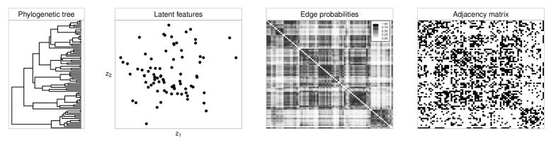
In this article we address the aforementioned gap by developing a novel phylogenetic latent space model (phylnet) for network data that explicitly characterizes the generative process of the nodes’ features via a branching Brownian motion, with branching structure parametrized by a phylogenetic tree (Felsenstein, 2004). As illustrated in Figure 1, this formulation crucially combines classical latent space representations of the edges in the network (Hoff et al., 2002) with a structured characterization of the features formation process inspired by the concept of continuous trait evolution from the phylogenetic literature. Extending this metaphor to network models, the formation of complex multiscale connectivity patterns can be viewed, under phylnet, as the result of node-specific latent features which evolved over a phylogenetic tree; this phylogenetic tree constitutes the main object of inference.
As clarified in Sections 2.1 and 2.2, the above interpretation is useful in providing intuitions on the proposed phylnet generative model, but in practice we leverage the proposed features’ formation process to induce and learn structured dependence among the nodes in the network through a flexible tree-based architecture that unveils increasingly-nested modular hierarchies among nodes, even when these hierarchies do not necessarily have an evolutionary interpretation. Although this direction is novel in the latent space modeling framework, we emphasize that tree-based constructions have appeared in generalizations of stochastic block models (e.g., Roy et al., 2006; Clauset et al., 2008; Roy and Teh, 2008; Herlau et al., 2012). However, the overarching focus has been on learning hierarchies between nodes or nodes’ partitions, under stochastic equivalence or more general homogeneity assumptions. Besides yielding substantially different models and tree-based representations, this perspective might fail to characterize heterogenous patterns at the node level and, as illustrated empirically in Section 4, it experiences challenges in networks without a clear block structure. Conversely, the proposed phylnet model flexibly characterizes broader network structures by modeling the features formation process directly at the node level. This perspective requires methodological and computational innovations also with respect to the classical literature on phylogenetic trees, since the node-specific features are not directly observed, but rather denote latent quantities which are identifiable only up to translations and rotations in latent space models (Hoff et al., 2002). In Section 2.2.1, we prove theoretically that, despite this identifiability issue at the latent features level, the main object of inference, i.e., the phylogenetic tree, remains still identifiable.
The above discussion clarifies that the proposed phylnet model can also lend itself naturally to extensions in different settings, including latent space representations for directed, bipartite, multilayer and multiplex/replicated networks. Section 2.3 pursues this direction with a focus on the latter class, which comprises multiple network observations, on the same set of nodes, encoding either different types of relationships (multiplex networks) or replicated measurements of the same notion of connectivity (replicated networks). In this context, we allow the latent features of each node to change across networks, but assume a shared phylogenetic tree regulating the formation process of these features in the different networks. This allows to borrow information among networks for estimating complex tree-based modular hierarchies among nodes, while preserving flexibility in characterizing network-specific multiscale structures. Within this setting we also prove theoretical consistency properties in learning the underlying phylogenetic tree as the number of networks increases; see Section 2.3.1.
In Section 3, we give details for posterior inference on the phylogenetic tree parameterizing the phylnet model in a Bayesian setting and under a pure-birth process prior for the tree. Combined with the latent space model likelihood, this prior induces a posterior distribution for the phylogenetic tree which we learn through a bespoke Metropolis-within-Gibbs algorithm. The tree samples produced by this algorithm are then summarized for both point estimation and uncertainty quantification via the notions of consensus tree (see, e.g., Felsenstein, 2004) and DensiTree (Bouckaert, 2010). Our simulation studies in Section 4 show that this fully Bayesian perspective provides remarkable performance improvements over both heuristic and model-based solutions for learning hierarchical multiscale structures in network data, including state-of-the-art generalizations of stochastic block models (e.g., Clauset et al., 2008). These gains are confirmed in applications to multiple corrupted measurements of a Mafia-type criminal network (Calderoni et al., 2017; Legramanti et al., 2022) (see Section 5.1), and to replicated brain network data observed from different individuals (Craddock et al., 2013; Kiar et al., 2017) (see Section 5.2). In the former case, phylnet unveils a previously-unexplored tree-based reconstruction of the organizational architecture of the Mafia group under analysis, and highlights criminals with highly peculiar positions within the hierarchy. In the latter, the inferred phylogenetic tree learns interesting nested symmetries in the human brain, while pointing toward a top-level frontal-back division of the brain followed by a nested partition in the two hemispheres. Future directions of research are discussed in Section 6. Proofs and additional results can be found in the Supplementary Material.
2 Phylogenetic Latent Space Models
Sections 2.1–2.3 present the proposed class of phylogenetic latent space models. As clarified in Section 1, this class relies on concepts from phylogenetic inference (reviewed in Section 2.1) to incorporate and learn meaningful structure underlying the generative process of the node-specific features in latent space models for network data. Section 2.2 formalizes the resulting phylnet formulation focusing first on a single network, and studies the identifiability of the underlying phylogenetic tree. This formulation is then extended to multiple networks in Section 2.3, where we also prove consistency properties for the posterior on the phylogenetic tree as the number of networks grows.
2.1 A brief introduction to phylogenetic trees
The phylogenetic trees we consider here are rooted, binary branching trees endowed with branch lengths. When studied probabilistically, these objects can be characterized as random trees with random branch lengths, or equivalently as point processes in the product space of time and tree-node indexes, or as branching processes (e.g., Aldous, 2001). By providing a natural and interpretable graphical representation of evolutionary relations among entities, these trees have been extensively studied and routinely employed in the field of evolutionary biology; see e.g., Felsenstein (2004) for an introduction. Nonetheless, more recent contributions have shown that the utility of these constructions extends beyond evolutionary biology, yielding successful implementations also in the fields of linguistics (Hoffmann et al., 2021; Ryder, 2025) and cultural evolution (Evans et al., 2021; Buckley et al., 2025), among others.
In Sections 2.2–2.3, we further extend the applicability and potentials of phylogenetic trees by leveraging these objects to characterize the formation process of node-specific latent features in models for network data. To this end, we consider trees having a fixed number of leaves (corresponding to the nodes in the network) and meeting the ultrametric property. This property is inherently motivated by the relevance of specific non-Euclidean geometries in latent space models for networks discussed in Section 1 (e.g., Smith et al., 2019), and means that all paths connecting the root to a leaf node have the same length, defined as the sum of the branch lengths. We perform inference on such a tree under the proposed phylnet model via a Bayesian approach. This perspective has witnessed growing interest in the phylogenetic tree literature (e.g., Chen et al., 2014). Not only does it facilitate inclusion of prior information, but it also allows for principled point estimation under sophisticated models, uncertainty quantification, and direct inference on complex functionals. In this framework, the tree is treated as a random object endowed with a prior distribution, often within the class of birth and death branching processes (e.g., Harris, 1963; Ross, 2014). Such a class includes as a special case the pure birth Yule process (Yule, 1925) which we employ as a prior for the tree structure in our construction. Notice that we restrict ourselves to binary trees, a common choice in phylogenetics. This is not a strong constraint, as a multifurcating tree can be approximated by a binary tree with very short branches. Moreover, the consensus trees we use as a summary of the posterior distribution need not be binary.
In classical evolutionary models, the above phylogenetic tree constitutes the branching architecture that regulates the formation of a certain character of interest across a set of entities, represented as the leaves of the tree. Often, this process is modeled as either a continuous or discrete state-space continuous-time Markov chain, depending on the nature of the character. In our phylnet model, the character denotes the real-valued latent features at the different nodes, thereby requiring a continuous state-space process. Motivated by its success in evolutionary modeling (e.g., Felsenstein, 1985; Eastman et al., 2011; May and Moore, 2020) we consider, in particular, a branching Brownian motion to provide a flexible, yet tractable, characterization of the features formation process over the architecture of the phylogenetic tree. This choice crucially yields a multivariate normal distribution for these features at the leaves, with a variance-covariance structure that reflects the phylogeny. More specifically, consider for simplicity the case in which each leaf is characterized by a single latent feature , and denote with the variance parameter of the Brownian motion. Let be the height of the tree, i.e., the distance between the root of the tree and any of its nodes. For any pair of nodes , let be the distance between the root and the most recent common ancestor to and ; a large value of means that and are close cousins. Then, under the branching Brownian motion model, the joint distribution of the features’ vector at the leaves of the tree is a multivariate Gaussian, i.e., with marginal variances and covariances . Hence, the “closer” and are in the phylogeny, the higher the covariance among the corresponding features. This means that, under this construction, tree-based representations of nested modular hierarchies among nodes can be possibly learned from the structure in the pairwise dependencies among nodes’ latent features. This intuition is at the basis of the phylnet model presented in Section 2.2 (see Chapter 4 in Felsenstein (2004) for more details on phylogenetic trees).
2.2 Model formulation for a single network
Although the proposed phylnet model can be readily extended to several network structures, including directed, bipartite and weighted settings, we focus here on the simplest, yet ubiquitous, case of a single binary undirected network. Let denote the symmetric adjacency matrix representation of such a network, so that if nodes and are connected, and otherwise, for . Consistent with classical latent space models for network data (Hoff et al., 2002), we assume
| (1) |
where is a scalar controlling the overall network density, while and are the vectors of latent features for nodes and , respectively, with denoting the Euclidean distance among the features vectors. The above representation embeds nodes in a -dimensional latent space with positions informing on edge probabilities. More specifically, the closer the features vectors of and , the higher the probability to observe an edge among these two nodes. As mentioned in Section 1, this natural interpretation has motivated a direct focus on the latent features as the main object of inference. To this end, routine implementations rely on independent Gaussian (Hoff et al., 2002) or mixtures of Gaussian (Handcock et al., 2007) priors for the nodes’ latent features and then provide inference on the induced posterior distribution. Although the latter perspective increases flexibility and inference potentials relative to the former, both solutions lack a structured and realistic characterization of dependence among the node-specific feature vectors, and still treat these vectors as the main object of interest. As such, inference reduces to graphical interpretations of a model-based embedding of the nodes, possibly grouped in dense communities under mixtures of Gaussian priors. In fact, one would expect that the latent features exhibit, in practice, structured dependence across nodes, with this dependence possibly unveiling more fundamental and informative architectures, such as increasingly nested modular hierarchies among nodes, at the basis of multiscale patterns in the network.
Motivated by the above discussion and recalling Section 2.1, we complement model (1) with a structured characterization of the features formation process via a branching Brownian motion parameterized by a phylogenetic tree that constitutes the main object of inference. Crucially, this advancement (i) facilitates improved reconstruction of the nodes embedding by explicitly borrowing information among the features of the different nodes and (ii) substantially enlarges inference potentials on core node hierarchies through the phylogenetic tree. More specifically, let be the matrix with generic row encoding the values of the -th feature for the different nodes, and denote with the (ultrametric) phylogenetic tree characterizing the branching architecture which regulates the features formation process. In this setting and conditional on , we assume independent branching Brownian motions (bbm) for the different features’ dimensions from to . Recalling Section 2.1, this implies that, at the leaf nodes,
| (2) |
where is the vector of all ones, denotes a centering parameter for the -th feature, is the bbm rate, while corresponds to the correlation matrix induced by the tree , as described in Section 2.1. In the applications we consider, the parameter has no clear interpretation and is not identifiable. Thus we fix , so that can be directly interpreted as the marginal variance of each , for , whereas denotes the correlation between and for any . Let us emphasize that setting does not constrain the prior specification in (2), nor it affects the tree branching topology.
To complete the Bayesian specification, we require priors for , and the tree in (2), along with the scalar in (1). Regarding and , notice that, under (2), the latent features are identifiable only up to translations and rotations (Hoff et al., 2002). As proved in the following, this issue does not affect the identifiability of the main object of interest, i.e., the tree , but it implies that the centering quantities in (2) can be treated as nuisance parameters. However, as highlighted in Section 3.1, including these quantities allows us to re-center the latent features at each step of the Metropolis-within-Gibbs routine we derive, and hence obtain improved mixing and convergence of the chain for . Consistent with this discussion, we consider diffuse Gaussian priors for and a conditionally conjugate inverse-Gamma prior for . More precisely, we let
| (3) |
Recalling Section 2.1, for the phylogenetic tree we consider a pure-birth Yule process prior (Yule, 1925), which can be obtained as a special case of birth and death branching processes (e.g., Harris, 1963; Ross, 2014) by setting the death rate . This yields
| (4) |
The above choice is common in phylogenetic inference, having the advantage of being both tractable and diffuse over the space of binary trees. This allows flexible Bayesian learning of different, possibly complex, tree architectures, while facilitating posterior computation.
Finally, for the scalar in (1), we follow standard practice (Hoff et al., 2002) and let
| (5) |
Model (1)–(5) formalizes the proposed phylnet representation and provides a flexible generative latent space characterization of complex multiscale network structures that unveil informative tree-based modular hierarchies among nodes encoded in . Learning this parameter under (1)–(5) is, in principle, possible by carefully combining results from classical latent space models for network data (Hoff et al., 2002) and Bayesian phylogenetic inference (see e.g., Chen et al., 2014). However, as previously discussed, unlike for classical evolutionary models, in the proposed phylnet formulation the tree regulates the formation of features that are not directly observed, but rather latent and identifiable only up to translations and rotations (Hoff et al., 2002). This motivates innovations in terms of posterior computation (see Section 3.1) and, more crucially, requires careful theory guaranteeing that inference on the phylogenetic tree parameterizing the formation process of the latent features is not affected by the identifiability issues of these features in the likelihood.
2.2.1 Identifiability of the phylogenetic tree
Consistent with the discussion above, Theorem 1 and Proposition 1 clarify that, despite the identifiability issues of the latent features, the tree and the rate of the Brownian motion remain identifiable. These two results rely on Lemmas 1–2 below, which state properties of direct interest for the broader class of latent space models for networks (Hoff et al., 2002), beyond the proposed phylnet representation. More specifically, Lemma 2 exploits a geometrical result for Euclidean distance matrices (Hayden et al., 1991) provided in Lemma 1, to show that the scalar and the matrix of pairwise distances are identifiable under model (1). Refer to the Supplementary Material for proofs.
Lemma 1.
Consider a Euclidean distance matrix which admits a representation in , i.e., there exist such that . Let be the minimum non-zero value in , i.e. . Let be the matrix defined as
| (6) |
for some and . Then, if , does not admit a representation in .
Lemma 2.
Consider the latent space model in (1) for the adjacency matrix , and let be the pairwise distance matrix having entries , for every . Then, if , the parameters and are identifiable. More precisely, denoting with the joint model for the edges in the adjacency matrix , it holds that,
| (7) |
for any couple of parameters and .
Although Lemma 2 states a relevant identifiability result for the broad class of latent space models, the tree and the rate of the Brownian motion do not parameterize directly, but rather the features that define the distances in . Theorem 1 and Proposition 1 combine the result in Lemma 2 with properties of binary trees and multivariate Gaussians to prove that and are also identifiable.
Theorem 1.
Although Theorem 1 guarantees identifiability of and under the marginalized model , in practice, the Metropolis-within-Gibbs routine presented in Section 3.1 samples also the latent features in to facilitate the derivation of tractable full-conditional distributions for and . However, as discussed previously, the latent features are identifiable only up to translations and rotations. In classical latent space models (e.g., Hoff et al., 2002; Handcock et al., 2007), where the focus of inference is specifically on these latent features, this issue is addressed through a processing step that aligns the samples of via Procrustean transformation. Crucially, this internal re-alignment is not required when the focus of inference is on and , as in the proposed phylnet model. More specifically, the translation aspect is addressed through the re-centering operated by the auxiliary parameters in (2). As for rotation, Proposition 1 guarantees that the conditional distribution of the zero-centered latent features given and is invariant with respect to orthogonal transformations.
Proposition 1.
Let be the matrix with rows distributed as in (2). Then, for any orthogonal matrix , it holds that , where .
2.3 Extension to multiple network measurements
Before deriving in Section 3 the Metropolis-within-Gibbs routine for inference under the proposed phylnet model, we generalize in this section the model formulation to the case of multiple adjacency matrices each encoding different connections among the same set of nodes. In this context, which includes modern settings of direct interest, such as multiplex and replicated networks (see, e.g., Gollini and Murphy, 2016; Durante et al., 2017; Salter-Townshend and McCormick, 2017; Wang et al., 2019; Arroyo et al., 2021; MacDonald et al., 2022), the proposed phylnet model not only admits a natural generalization, but also benefits from the multiple network measurements to achieve an improved reconstruction of the underlying tree , with theoretical guarantees of posterior consistency.
Consistent with other extensions of latent space models to multiplex and replicated network settings (see e.g., Gollini and Murphy, 2016; Durante et al., 2017; Salter-Townshend and McCormick, 2017; Wang et al., 2019; Arroyo et al., 2021; MacDonald et al., 2022), we generalize the proposed phylnet model in a way that achieves flexibility in modeling differences among multiple network measurements , while learning relevant shared structures. Since the nodes are common to the different networks, within our novel framework it is natural to expect that the architecture (i.e., the tree ) underlying the features formation process is shared among , with the differences among these adjacency matrices being the result of network-specific features evolving over the shared tree architecture. Motivated by these considerations, we let
| (9) |
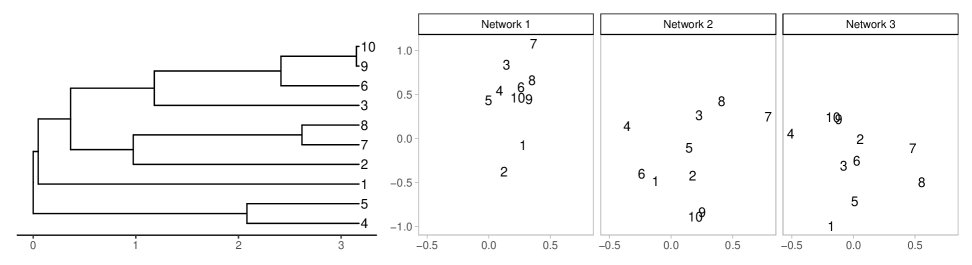
independently for each , where , with , while and denote the vectors of latent features for nodes and , respectively, in the -th network. As discussed above, these features are allowed to change across networks in order to flexibly characterize differences in the edge probabilities between the multiple adjacency matrices through a formation mechanism regulated by a shared tree-based architecture (see Figure 2 for a graphical example with ). Extending (2)–(5) to the multiple networks setting, this yields
| (10) |
where the centering parameters , and rate have independent priors
| (11) |
while the tree and the scalar are assigned the same priors as in Section 2.2, namely
| (12) |
Model (9)–(12) is an effective extension of the proposed phylnet construction to multiple networks (note that this extension can be made even more flexible, without major complications from a computational perspective, by letting both and be network-specific, i.e., and ).
2.3.1 Posterior consistency for the phylogenetic tree
Model (9)–(12) not only achieves flexibility in modeling multiple network measurements, but also benefits from these measurements to gain efficiency in inference on the shared tree . This property is formalized in Theorem 2 which states consistency for the posterior distribution on as .
Theorem 2.
Let a phylogenetic tree be decomposed into the respective tree topology , where is the space of binary tree topologies with terminal nodes, and the collection of branch lengths satisfying the ultrametric property. Then, it holds that , there exists with , such that if i.i.d. with , then for any neighborhood of ,
| (13) |
where is the conditional distribution of under the prior (11)–(12).
The proof of Theorem 2 can be found in the Supplementary Material and exploits the finiteness of the space of tree topologies with nodes, together with Doob’s consistency theorem (Doob, 1949; Ghosal and Van der Vaart, 2017) and the identifiability results in Section 2.2.1. Albeit stated for a single adjacency matrix, these identifiability results directly extend to the multiple networks setting.
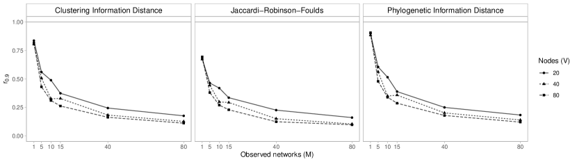
Although Theorem 2 provides strong theoretical support to the proposed phylnet construction, the consistency result stated is asymptotic in nature. In practice, is finite and, hence, it is of interest to assess whether the theoretical consistency translates into empirical evidence of effective concentration for the posterior of around a true tree . To answer this question, we simulate networks from model (9)–(11) for different settings of and , letting and true underlying tree architecture drawn from prior (12). Conditioned on these networks, we sample multiple trees from the corresponding posterior distribution, as detailed in Section 3.1, and then leverage such samples to monitor the concentration of the posterior around as grows, for different settings of , via the radius of the credible sets centered at ; see Figure 3. These credible sets contain the sampled trees closest to according to the three important notions of normalized tree distance (i.e., the Clustering Information Distance (Smith, 2020a), the Jaccardi–Robinson–Foulds (Böcker et al., 2013) and the Phylogenetic Information Distance (Smith, 2020a), as implemented in the R package TreeDist (Smith, 2020b)), whereas the radius coincides with the maximum of the distances between and the trees in the credible set. As illustrated within Figure 3, the radius progressively shrinks as grows, for any , meaning that the posterior increasingly concentrates around , thereby providing empirical support in finite- settings to Theorem 2. Notice that the larger radius at is due to the fact that, in this setting, the model has only latent features for each node to learn a complex tree structure. This translates into higher posterior uncertainty. This result does not mean that reasonable point estimates of the tree cannot be obtained when , but rather clarifies that the proposed phylnet construction is able to properly quantify posterior uncertainty.
3 Posterior Computation and Inference
Due to the intractability of the posterior distribution induced by model (9)–(12), we design in Section 3.1 a Metropolis-within-Gibbs procedure targeting this posterior. This routine samples iteratively from the full-conditional distributions of the model parameters either via conjugate updates or through Metropolis–Hastings steps with tailored Gaussian proposals, except for which requires suitable tree moves. Notice that, although our overarching focus is on the posterior distribution for , as illustrated in the following, it is practically more convenient to implement a routine targeting the full posterior induced by model (9)–(12), and then retain only the samples of to perform inference on the marginal posterior for the tree as detailed in Section 3.2.
3.1 Posterior computation via Metropolis-within-Gibbs
In the following, we detail the steps of the proposed Metropolis-within-Gibbs algorithm for a generic ; setting yields directly the sampling strategy for the single-network phylnet model in (1)–(5).
Focusing first on the scalar , its full-conditional distribution
lacks conjugacy between the Gaussian density and the model likelihood, thereby requiring a Metropolis–Hastings update. This update relies on a random walk Gaussian proposal with variance tuned as in Andrieu and Thoms (2008) to target the ideal acceptance rate of , which ensures an effective balance between local and long-distance exploration of the parameter space. In practice, this is achieved by defining the standard deviation of the Gaussian proposal at step as , where denotes the acceptance probability at iteration .
The above tuning step is implemented not only for the parameter , but also for all the quantities in model (9)–(12) sampled via Metropolis–Hastings updates relying on Gaussian proposals. This is the case, in particular, of the latent features encoded in the matrix , for , whose full-conditional is
for each . Crucially, this form allows us to implement parallel Metropolis–Hastings updates for over , with each parallel update sampling jointly the -dimensional features vector of every node , for .
Given samples for , the rate parameter and the centering quantities , , , admit conjugate inverse-Gamma and Gaussian full-conditionals, respectively. More specifically, let and , then
for every and , where , with . Adapting state-of-the-art implementations of classical latent space models (Krivitsky et al., 2009), the above updates are also combined with a subsequent step re-sampling jointly under a Metropolis–Hasting scheme aimed at further improving mixing. More specifically, this mixing improvement is accomplished by proposing a jointly-rescaled version of the previously-sampled values for , and , with , and then accepting or rejecting the proposed rescaled vector based on the corresponding Metropolis–Hastings acceptance probability. Similarly to Krivitsky et al. (2009), we also found this additional step to be effective in practice.
In order to sample from the full-conditional of , we adapt strategies available in the literature on Bayesian phylogenetic trees (e.g., Kelly et al., 2023; Chen et al., 2014) treating the sampled feature vectors as the observed traits. More specifically, we rely on Metropolis–Hastings updates based on five symmetric moves that ensure ergodicity of the chains in the tree space. These moves are:
-
•
Tips interchange: for each leaf node randomly select another leaf and swap them;
-
•
Subtree exchange: randomly select two subtrees and swap them;
-
•
Tree-node age move: randomly select an internal node and shift its age, corresponding to the expansion or contraction of the branches connecting the selected node, its parent in the tree and the child nodes, keeping unchanged the total height of the tree;
-
•
Subtree pruning and regrafting (spr): randomly select a subtree, prune it and re-attach the resulting subtree to another suitable position in the tree;
-
•
Local-spr: spr move with the restriction of regrafting in any suitable branch of the subtree rooted at the parent node of the pruned subtree.
To enhance mixing and convergence, we follow recommended practice in Bayesian phylogenetics and implement all the above moves for a pre-specified number of times in each step of the Gibbs routine, while checking that the proposed move does not violate the ultrametric property of the resulting tree.
Finally, given the sample of the tree , the associated prior hyperparameter is drawn via a random walk Metropolis–Hastings update from the full conditional
where denotes the density of a birth and death process with rates and computed at the tree . In this case we propose again from a Gaussian.
The above Metropolis-within-Gibbs routine is initialized with random draws from the prior for all parameters, except for whose starting value is set at the median of the mle estimates provided by different latent space models (Hoff et al., 2002) fitted separately via the R-package latentnet (Krivitsky and Handcock, 2008) to each observed network . Notice also that the sampling steps discussed above are performed in random order within each full cycle of the Metropolis-within-Gibbs routine. In our experience, this choice helped to further improve mixing.
3.2 Posterior inference on
As mentioned in Section 1, the architecture of the phylogenetic tree allows us to unveil increasingly-nested modular hierarchies among nodes that inform on multiscale network structures often observed in practice. This motivates our overarching focus on posterior inference for such an architecture, via the posterior samples for produced by the Metropolis-within-Gibbs routine outlined in Section 3.1.
To address the above endeavor, we use point estimation and uncertainty quantification techniques specifically devised for inference within complex tree spaces (e.g. Felsenstein, 2004). We rely, in particular, on two standard summaries of the sample of trees, known as DensiTree and consensus tree (see Figures 7 and 9). A DensiTree (Bouckaert, 2010) allows full visualization of the posterior uncertainty, by overlaying all the trees in the sample under a common ordering of the leaves. This is a highly useful visualization, but can sometimes be so blurry as to be difficult to interpret. A consensus tree, on the other hand, summarizes the posterior via a single tree. This is accomplished by displaying only those splits which appear within the sampled trees in a proportion above a threshold . As a result, some internal nodes of the consensus tree may be multifurcating when no split has high enough empirical posterior probability, thereby facilitating the identification of those parts of the tree that are uncertain or poorly-resolved in the posterior distribution. The branch lengths of the consensus trees are computed as the mean of the lengths of the corresponding branches in the tree samples.
4 Simulation Studies
We assess the performance of the proposed phylnet model and its empirical improvements over alternative competitors in two simulation scenarios that exhibit different network structures. In our first simulation scenario (illustrated in Figure 4), there is no multiscale pattern. In particular, we consider networks with nodes whose connections are sampled from independent Bernoulli variables having edge probabilities that display community-type architectures among 5 groups, with no evidence of multiscale patterns. In our second simulation scenario, we consider instead networks of size simulated under the data generative process of the phylnet model discussed in Section 2.3. More specifically, we first generate the true underlying tree from the prior in (12) with . Conditioned on this tree, the node-specific latent features are simulated, across the networks, from (10), setting and , for all and . Finally, conditionally on these simulated features, the edges in the adjacency matrices are generated from the latent space model in (9), with . Figure 5 provides a graphical illustration of , along with the expectation of the edge-probability matrices and examples of three simulated adjacency matrices in the second scenario. Unlike the first scenario, in this case the nodes display heterogeneous and nuanced multiscale patterns, thereby allowing to assess the phylnet construction both in situations where networks are not simulated from the generative process underlying the proposed model (first scenario) and also in correctly-specified, yet highly-challenging, settings (second scenario).
Posterior inference under the phylnet model proceeds via the Metropolis-within-Gibbs algorithm outlined in Section 3.1, setting , and . Although in our experiments the phylnet model proved robust to moderate deviations of such hyperparameter settings, these default values have always led to sensible results when applied to substantially different networks in simulations and applications. Regarding the choice of , we implemented separate latent space models as in Hoff et al. (2002) (using the latentnet R–package) for each of the simulated networks in both scenarios to explore how different settings for were able to characterize the structure of the different observed networks. This procedure led to select , which was shown to achieve a sensible balance between dimensionality reduction and goodness-of-fit. For both scenarios, posterior inference relies on 4 chains of iterations, with a burn-in window of 75,000 and a thinning every 50 iterations, as suggested by mcmc diagnostics. Note that these conservative mcmc settings are common in Bayesian phylogenetic inference, due to the complex topology of tree spaces (e.g., Chen et al., 2014).
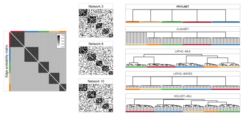
Figures 4–5 display the consensus trees (see Section 3.2) obtained under the proposed phylnet model, for both the first and second simulation scenarios, respectively. To further clarify the empirical gains of phylnet, these architectures are also compared with alternative tree-based reconstructions of the multiscale patterns underlying the simulated networks. As discussed in Section 1, current literature comprises some generalizations of stochastic block models to learn tree-structured node hierarchies (e.g., Clauset et al., 2008), but lacks solutions that can infer heterogenous tree-based generative mechanisms in latent space models. To this end, we consider as competitors the model by Clauset et al. (2008) (clauset), a simple hierarchical clustering which uses the sum of the adjacency matrices as a similarity matrix (hclust-adj), and two heuristic implementations of our general idea (lathc-mle and lathc-bayes). The first (lathc-mle) relies on a maximum likelihood estimate of the nodes’ latent features obtained via the latentnet R–package (Hoff et al., 2002), with , and then applies hierarchical clustering to infer a dendrogram that encodes tree-based similarity patterns among the features of the different nodes. The second (lathc-bayes) employs the same idea, but applied to the posterior samples of the nodes’ latent features produced again by the latentnet R–package under the Bayesian latent space model (Hoff et al., 2002). This induces a posterior distribution over the resulting dendrograms that is summarized via a consensus tree. Note that latent space models (Hoff et al., 2002) and the method by Clauset et al. (2008) are originally designed for a single network. Hence, these formulations are applied to the weighted network that arises from the sum of the binary adjacency matrices, thereby requiring a binomial likelihood for the counts of edges between each pair of nodes.
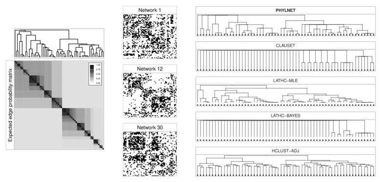
The visual comparison in Figures 4–5 among the tree inferred by the phylnet model and those obtained under the aforementioned competitors highlights the noticeable empirical gains achieved by phylnet in learning complex tree-based structures behind different networks. Although the networks in the first scenario are not simulated under the phylnet data-generative mechanism, it is sensible to expect that a suitable tree-based representation for the corresponding block structures would combine a root multifurcation into the five different communities with additional nested multifurcations of the nodes within each of these communities, compressed at the terminal leaves. Such a compression would correctly indicate that nodes within each community are stochastically equivalent (e.g., Nowicki and Snijders, 2001), and hence indistinguishable in terms of connectivity behavior. While all the methods under analysis properly learn the node communities in the first scenario, as is clear from Figure 4, phylnet aligns more closely with this expected tree-based representation of the resulting community structures. The empirical improvement in learning nested modular hierarchies among nodes is evident also in Figure 5 when comparing the consensus tree inferred by phylnet with the true underlying the simulation of the multiple networks in the second scenario. Table 1 quantifies these gains through the distances between the inferred trees and the true , under the metrics discussed in Section 2.3.1 (Jaccardi–Robinson–Foulds (Böcker et al., 2013); Clustering Information Distance (Smith, 2020a), and Phylogenetic Information Distance (Smith, 2020a)). More specifically, we compute the distance between and its point estimate under the non-Bayesian methods (lathc-mle, hclust-adj), while for the Bayesian solutions (phylnet, clauset, lathc-bayes) we consider a more in-depth assessment of posterior concentration. This is accomplished by computing the distance of from each posterior sample of , and then displaying the empirical average of the resulting distances along with the associated quantiles 0.05 and 0.95.
| Distance | phylnet | clauset | lathc-mle | lathc-bayes | hclust-adj |
|---|---|---|---|---|---|
| jrf | 0.18 [0.13,0.21] | 0.44 [0.36,0.50] | 0.33 | 0.42 [0.37,0.48] | 0.53 |
| cid | 0.22 [0.16,0.26] | 0.58 [0.45,0.63] | 0.34 | 0.47 [0.41,0.52] | 0.54 |
| pid | 0.22 [0.17,0.27] | 0.61 [0.49,0.67] | 0.34 | 0.49 [0.43,0.55] | 0.55 |
The results in Table 1 confirm the superior performance of phylnet in achieving substantially-improved posterior concentration around the true . This is not the case for the model by Clauset et al. (2008) (clauset) that displays performance similar to a simple hierarchical clustering applied to the sum of the adjacency matrices (hclust-adj). This behavior is arguably attributable to the fact that clauset was originally developed as a tree-based extension of stochastic block models, and hence fails to characterize more heterogenous node-specific patterns captured by latent space representation. This is further evident in the slight performance gains displayed by the heuristic versions of our novel idea (i.e., lathc-mle and lathc-bayes) which, unlike for clauset, leverage latent space model representations. However, the performance of these heuristics is much poorer than that of phylnet. Such a result motivates two comments. First, this gain is reminiscent of a well-known effect in phylogenetics, where evolution-based models tend to improve upon distance-based methods such as UPGMA or neighbor-joining (Felsenstein, 1981; Hillis et al., 1994; Kuhner and Felsenstein, 1994). Second, these heuristics do not benefit from a fully-Bayesian specification and coherent uncertainty quantification. This is particularly evident for lathc-bayes that may lack coherent tree structure across posterior samples of the latent features, thereby leading to poorly-resolved consensus trees (see Figure 5).
The above empirical gains of phylnet are further complemented by credibile intervals for its continuous parameters that contain the true values employed in the simulation (i.e., , , ). More specifically, the inferred credible intervals for , and in the second scenario are , and , respectively. In Section 5, we thus move on to two challenging applications from criminology and neuroscience, and illustrate further the ability of phylnet to learn tree-based node architectures underlying real-world network data.
5 Applications
The empirical results in the simulation studies within Section 4, together with the identifiability and posterior concentration properties presented in Section 2, confirm the ability of the proposed phylnet model to infer informative tree-based node hierarchies from complex multiscale connectivity patterns, thereby motivating its implementation in the two applications outlined in Sections 5.1–5.2.
5.1 Criminal networks
There is a substantial interest in criminology on unveiling the nuanced organizational structures of criminal networks from the analysis of the complex connectivity patterns among the corresponding members (see, e.g., Calderoni et al., 2017; Coutinho et al., 2020; Campana and Varese, 2022). Current attempts at addressing this fundamental goal are constrained by the lack of network models capable of learning the complex multiscale architectures underlying highly-structured criminal organizations, and by the challenges that arise from combining the multiple noisy data sources available (including separate investigations from different law-enforcement agencies) (e.g., Bright et al., 2022; Diviák, 2022).
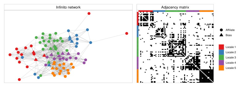
Consistent with the above discussion, we consider the proposed phylnet model within a hypothetical, yet realistic, scenario based on data from a large law enforcement operation conducted in Italy from to for monitoring and then disrupting a highly-structured ’Ndrangheta mafia organization in the area of Milan. To this end, we consider, in particular, the dataset studied recently by Legramanti et al. (2022) and Lu et al. (2025) which comprises information on the participation of criminals to monitored summits of the criminal organization, as reported in the judicial documents. Legramanti et al. (2022) and Lu et al. (2025) map this information into a single network with edges denoting either dichotomized (Legramanti et al., 2022) or weighted (Lu et al., 2025) co-attendances among each pair of criminals to the monitored summits. Motivated by the above considerations, we consider instead an hypothetical scenario in which each of law-enforcement agencies has monitored a different subset of summits sampled a random and with replacement from the total of . This yields adjacency matrices with entries if criminals and co-attended at least one of the summits monitored by agency , and otherwise, for , . Since criminal network data are often prone to data quality issues (e.g., Diviák, 2022), we also add a level of contamination within each adjacency matrix by flipping of its edges. Figure 6 illustrates graphically one of these adjacency matrices, which we jointly model under the proposed phylnet construction. Although the scenario explored is hypothetical, this choice is useful in clarifying how separate investigations subject to data incompleteness and possible contamination, could be eventually pooled under phylnet to obtain an informative tree-based reconstruction of the organizational structure of the monitored Mafia group.
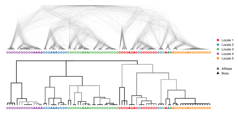
Figure 7 illustrates the output of this analysis through the DensiTree and consensus tree learned by the proposed phylnet model with the same hyperparameters and mcmc settings as in the simulations studies in Section 4. Interestingly, these trees reveal yet-unexplored hierarchies of increasingly-nested macro, meso and micro modules attributable to locali differentiations, role specialization within locali, and blood-family ties, respectively. Besides providing novel quantitative support to criminology theories on the organizational structure of the ’Ndrangheta mafia (e.g., Paoli, 2007; Catino, 2014; Calderoni et al., 2017), this unique tree structure also unveils specific criminals with more nuanced positions that partially depart from those of the more rigid ’Ndrangheta architecture. This is the case, for example, of the two affiliates within the clades of bosses from the blue and green locali. According to the judicial documents, these affiliates are high-rank members of the organization with a central role in overseeing the implementation of bosses’ decisions. Consistent with the learned trees, such a role is closer to the one covered by a boss than an affiliate. It is also interesting to notice three bosses of different locali form a subtree with the clade corresponding to the orange locale. Although this positioning might appear unusual, in the judicial documents these bosses are listed among those supporting a failed attempt to increase the independence of the ’Ndrangheta group in the area of Milan from the leading families in Calabria. The inferred tree suggests that this failed attempt resulted in a need for these bosses to move away from the corresponding locale and move their area of influence towards the orange one. This movement is also followed by closely-related affiliates. These results clarify the ability of phylnet to learn not only higher-level modular hierarchies within the network, but also more nuanced lower-level heterogenous behaviours of specific nodes, thereby achieving an effective balance between the rigid high-level organizational structure of ’Ndrangheta and the more fluid local positioning of its members.
5.2 Brain networks
State-of-the-art studies in neuroscience highlight the presence of symmetries and multiscale modular patterns in the organization of structural brain connectivity networks (Bullmore and Sporns, 2009; Meunier et al., 2010; Rubinov and Sporns, 2010; Bullmore and Sporns, 2012; Betzel and Bassett, 2017; Esfahlani et al., 2021). These findings are supported by a combination of anatomical considerations and empirical evidences from the analysis of replicated structural brain network data via community detection algorithms or stochastic block models (e.g., Meunier et al., 2010). However, although useful for identifying brain modules, both community detection and stochastic block models are not originally designed for inferring increasingly-nested hierarchies and symmetries among modules from the observed multiscale structures within human brain networks. As a result, current quantitative analyses might provide an overly-coarsened reconstruction of brain organization that fails to characterize complex modules at different scales along with heterogenous patterns at the level of brain regions.
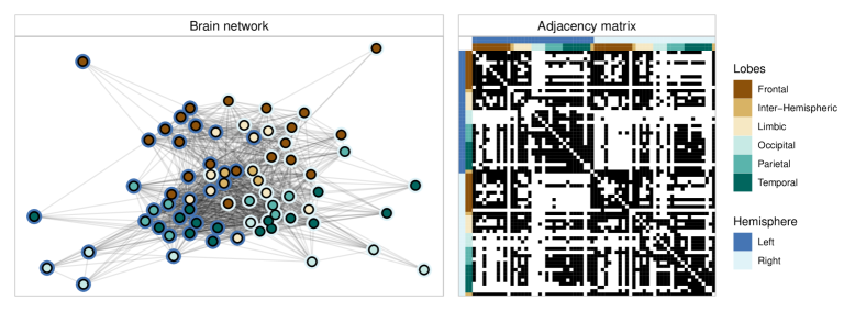
Motivated by the above discussion, we apply the proposed phylnet model to structural brain connectivity networks from the Enhanced Nathan Kline Institute Rockland Sample project. The pre-processed data are available at https://neurodata.io/mri/ and comprise white matter fibers connectivity measures among pairs of anatomical regions from the Desikan atlas (Desikan et al., 2006) for individuals whose brain has been scanned twice via diffusion tensor imaging (dti). We represent these data as binary adjacency matrices with generic entry if at least one white matter fiber is recorded among brain regions and in the two dti scans of individual , and otherwise, for , ; see Figure 8 for representative examples of the resulting adjacency matrices.
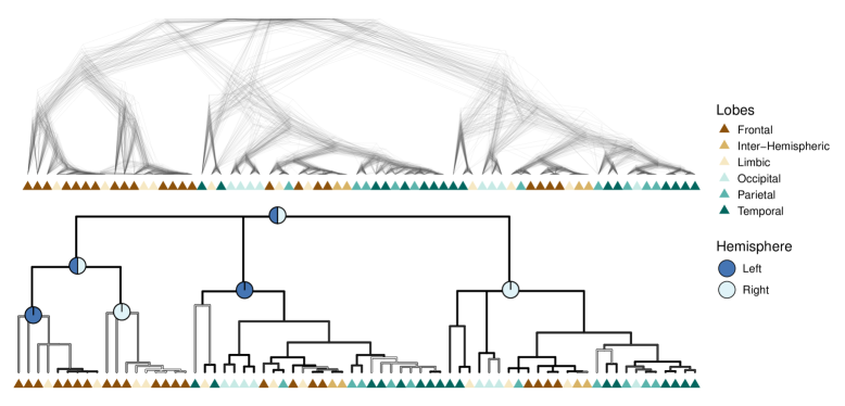
Figure 9 displays the DensiTree and consensus tree inferred by the phylnet model under the same hyperparameters’ specification and mcmc settings as in the simulation studies in Section 4. These trees unveil a previously-unexplored representation of the nested symmetries and hierarchies in brain organization that points toward a macro-level frontal-backward partition followed by an intermediate nested division according to the two hemispheres and a local-level organization which is generally coherent with lobes classification and crucially respect bilateral symmetries for those pairs of nodes characterizing the same region in the two different hemispheres. Interestingly, these symmetries are preserved also for those regions whose inferred position in the tree departs from lobe classification. For example, the two left and right regions from the limbic lobe allocated to the frontal clade (i.e., rostralanteriorcingulate and caudalanteriorcingulate) are anatomically closer to the anterior part of the human brain than other regions from the frontal lobe, such as the paracentral, precentral, caudalmiddlefrontal and part of the superiorfrontal which, in fact, are assigned to the backward clade under the phylnet model. Within the backward clade it is also interesting to notice three brain regions (i.e., temporalpole, entorhinal, parahippocampal) that form a peculiar branch that is present in both the left and right hemisphere division. Besides being spatially closer, these regions are conjectured to be closely-related both anatomically and functionally (Blaizot et al., 2010). The inferred tree in Figure 9 seems to provide empirical evidence in favor of this conjecture, while also aligning with recent analyses of brain modules that point toward the macro-level frontal-backward, rather than left-right, division of structural brain networks (Esfahlani et al., 2021). In addition to these analyses, the tree inferred in Figure 9 clarifies that the modular hierarchies and symmetries in human brains are more complex and nuanced than current classifications of brain regions into lobes, thus motivating future research on the definition of anatomical brain parcellations and taxonomies. These results are further strengthened by the DensiTree in Figure 9 that showcases a relatively low variability of the posterior for the phylogenetic tree, meaning that the inferred structures are generally stable and coherent across the studied individuals.
6 Conclusions
Although there is increasing evidence from several fields that real networks display multiscale structures and hierarchical organization (e.g., Ravasz and Barabási, 2003; Gosztolai and Arnaudon, 2021), state-of-the-art latent space models for network data still lack extensions capable of incorporating and learning these core and recurring architectures. We address this gap through a structured representation of the generative process underlying the nodes’ latent features that creates a unique bridge with Bayesian phylogenetics. This is accomplished by characterizing the nodes’ latent features via a branching Brownian motion parameterized by a phylogenetic tree that infers network hierarchical organization from the observed multiscale heterogenous connectivity patterns among nodes. As clarified in Sections 2–3, the resulting formulation guarantees the identifiability of the tree alongside posterior consistency properties in multiple network settings, and facilitates the implementation of a carefully-designed Metropolis-within-Gibbs algorithm for posterior inference. The empirical results in Sections 4–5 show that the proposed model can reconstruct informative and yet-unexplored tree-based representations of complex network organization in several settings displaying substantially different multiscale connectivity architectures.
The above advancement motivates several directions of future research. An important one is to extend the proposed phylnet model from binary undirected settings to directed and weighted network contexts. Both extensions require straightforward modifications of the proposed construction. In the former case it suffices to consider two vectors of latent features for each node regulating its sender and receiver behavior, and then learn two separate phylogenetic trees characterizing the formation process of these sender and receiver features, respectively. Inclusion of weighted edges simply requires to replace the Bernoulli likelihood with, e.g., a Poisson one and consider a latent space construction for the associated log-rates, rather than for the logit of the edge probabilities. A more challenging avenue of future research would be to include and learn a similar tree architecture for the formation of the grouping structures that parameterize a stochastic block model.
As discussed in Sections 2.2–2.3, the phylnet model benefits from the availability of multiple network observations to achieve effective Bayesian learning on tree-structured network organization. In fact, the diffuse prior on the tree combined with the complexity of this object have the effect of limiting posterior concentration when a single network is observed. One possibility to address this challenge is to supervise the prior on the tree via external node attributes that are often available in practice and generally inform on network connectivity. This perspective is equivalent to joint modeling of the node latent features and the node attributes as processes over the same tree , thereby augmenting the amount of signal from the data necessary to infer the tree. We have partially explored this direction and we obtained promising preliminary results which encourage further investigation in the future. Another interesting option is to capitalize on field knowledge to provide an evolutionary interpretation of network organization, whenever available. This would facilitate the specification of more informative priors for the tree and the features’ formation process that are coherent with the evolutionary assumptions of the network structures under analysis.
Note that, in our novel framework, the prior on the tree and the branching Brownian motion allow for the out-of-sample continuation of the tree growth process together with the evolution and formation of features, possibly accommodating new nodes entering network via the creation of additional branches or existing nodes exiting the network through pruning of the available branches from the tree. This opens new avenues for the out-of-sample projection of the growth process for the observed network.
Finally, from a more practical perspective, it is of interest to consider further research and studies on the specification of the latent space itself. To this end, particularly relevant is the choice of the number of features , which we address in the article by inheriting common-practice and goodness-of-fit analyses in classical latent space models (Hoff et al., 2002; Handcock et al., 2007; Krivitsky and Handcock, 2008). As such, any advancement along these lines (e.g., Kaur et al., 2023) can be readily employed under the proposed phylnet model. In addition, inspired by recent research on alternative latent space geometries (Smith et al., 2019), we believe it would be of interest to study the possibility of specifying the phylogenetic latent position model under non-Euclidean geometries. In this respect, a relevant direction would be to explore the hyperbolic latent space (Krioukov et al., 2010; Lubold et al., 2023), as this choice seems to naturally accommodate tree-like structures in the represented networks.
Acknowledgments
Federico Pavone is funded by the European Union’s Horizon 2020 research and innovation programme under the Marie Skłodowska-Curie grant agreement No 101034255. Daniele Durante is funded by the European Union (ERC, NEMESIS, project number: 101116718). Robin J. Ryder is funded by the European Union under the GA 101071601, through the 2023–2029 ERC Synergy grant OCEAN. Views and opinions expressed are however those of the author(s) only and do not necessarily reflect those of the European Union or the European Research Council Executive Agency. Neither the European Union nor the granting authority can be held responsible for them.
Supplementary Material
S1 Proofs
Below we provide the proofs of the theoretical results in the main article. To this end, let us first state and prove two useful lemmas.
Lemma S1.1.
Consider prior (10) for the features , and . Then, conditionally on and , it holds
independently over , where is the squared Euclidean distance between the -dimensional feature vectors of nodes and in network , and is a Chi-square with degrees of freedom.
Proof of Lemma S1.1.
Recall that under prior (10), we have
| (S.1) |
independently for and . Therefore, leveraging standard properties of multivariate Gaussian distributions, we have that
| (S.2) |
and, hence,
| (S.3) |
independently for and . Therefore, since , by the properties of the Chi-square distribution, it holds
| (S.4) |
independently over , thereby proving Lemma S1.1. ∎
Lemma S1.2.
Consider a set of indices representing the leaves of two binary splitting trees and . There always exists a pair of indices such that their most recent common ancestor is the root in both trees and .
Proof of Lemma S1.2.
The root bifurcation can be represented by a bipartition of in two non-empty complementary sets, which we refer to as for , and for . We want to show that we can always find a pair of indices , such that and . To this end, notice that there are only two possible scenarios representing the relations between the two partitions and . In one case, the following holds
| (S.5) |
and we can choose and , which satisfy the required condition. If (S.5) does not hold, we can assume without loss of generality that and hence . In this case, it must hold that
| (S.6) |
and we can choose and , which satisfy the required condition. ∎
Leveraging the above results, let us now prove Lemmas 1–2, along with Theorems 1–2 and Proposition 1 in the main article.
Proof of Lemma 1.
The proof is constructed considering two cases: and .
-
Case 1. . Consider the centering matrix , where is the matrix of all ones. Notice that . The Gram matrix associated to the matrix of squared distances can be written as
(S.7) Observe that , where is the element–wise square root of . Since, , the Gram matrix associated to can be written as
(S.8) where is the Gram matrix associated to the squared root distance . Since is Euclidean, then is Euclidean (Schoenberg, 1937; Maehara, 2013) and therefore is positive semidefinite. It follows that is positive semidefinite as all three terms in the right–hand–side of (S.8) are positive semidefinite. Hence, is a Euclidean distance matrix.
Now, recall that the Schoenberg criterion (Schoenberg, 1935; Maehara, 2013) states that is representable in if and only if . We now show that if is large enough, then and therefore does not admit a representation in . First of all, notice that by construction the vector of all ones is an eigenvector with eigenvalue 0 for both and . Since is representable in , then . Thus, there exist vectors such that . Moreover, because of orthogonality to . Consider now,
(S.9) We show that for all , the vector does not belong to the kernel of . Indeed,
(S.10) But since is positive semidefinite, it cannot have a negative eigenvalue equal to . Therefore, there are at least orthogonal vectors in . Hence, . Since is upper bounded by , for any it holds that .
-
Case 2. . This case is proven by contradiction. To this end, let us assume that admits a representation in . Then, under (6), can be written as with . Leveraging this result and the arguments of Case 1, it follows that, if , does not admit a representation in . This is a contradiction, because admits a representation in by construction. Hence, does not admit a representation in if .
∎
Proof of Lemma 2.
Under (1), the joint distribution of the edges in is identified by the Bernoulli probabilities , , , which in turn depend on and , under the 1-to-1 logit mapping, via the predictor . Therefore, the assumption
| (S.11) |
implies that for every , . Without loss of generality, we can assume , for some constant . Hence, in order for the equality to hold, we need that which implies . If , with , then would have at least one negative entry and it would not be a pairwise distance matrix. Otherwise, if , by Lemma 1, this is not possible as would not be representable in . ∎
Proof of Theorem 1.
We prove the result by showing that if , then
| (S.12) |
Leveraging Lemma S1.1 and defining , we can write the probability of a success in the marginal model as
| (S.13) |
where , while the expectation is computed with respect to and , i.e., the prior distributions. In order to prove (S.12), we show that for at least one pair the probability of an edge between and is different under the two parametrizations. In particular, when we can always choose such that as follows:
-
•
If , then from Lemma S1.2 there exists such that the two nodes split at the root in both and . Therefore , and, hence
(S.14) -
•
If and , then there exists such that . Therefore,
(S.15)
Without loss of generality, assume that . This implies
for any . Therefore, for the pair of nodes , it follows
for any , thereby proving Theorem 1. ∎
Proof of Proposition 1.
First notice that, under (2), is distributed as a matrix-normal. Specifically, . Therefore, leveraging standard properties of matrix-normal distributions, we have that
Since is an orthogonal matrix, it holds , which implies . ∎
Proof of Theorem 2.
Theorem 2 is a direct consequence of Doob’s consistency (Doob, 1949) and the finiteness of the space of binary tree topologies. Following the identifiability of for the marginal model proved in Theorem 1, Doob’s consistency theorem guarantees posterior consistency almost surely with respect to the prior , where .
Denote with the subspace of parameters for which posterior consistency holds everywhere due to Doob’s, i.e. where denotes the joint prior on defined in Section 2.3 of the main article. It follows that
| (S.16) |
where is the indicator function. Since , , due to the full support of the prior we consider, (S.16) implies that
| (S.17) |
Therefore, it follows that . Finally, one can choose , for which it holds that and that . ∎
References
- Airoldi et al. (2008) Airoldi, E. M., Blei, D., Fienberg, S., and Xing, E. (2008), “Mixed membership stochastic blockmodels,” Journal of Machine Learning Research, 9, 1981–2014.
- Aldous (2001) Aldous, D. J. (2001), “Stochastic models and descriptive statistics for phylogenetic trees, from Yule to today,” Statistical Science, 16, 23–34.
- Andrieu and Thoms (2008) Andrieu, C., and Thoms, J. (2008), “A tutorial on adaptive MCMC,” Statistics and Computing, 18, 343–373.
- Arroyo et al. (2021) Arroyo, J., Athreya, A., Cape, J., Chen, G., Priebe, C. E., and Vogelstein, J. T. (2021), “Inference for multiple heterogeneous networks with a common invariant subspace,” Journal of Machine Learning Research, 22, 6303–6351.
- Athreya et al. (2018) Athreya, A., Fishkind, D. E., Tang, M., Priebe, C. E., Park, Y., Vogelstein, J. T., Levin, K., Lyzinski, V., Qin, Y., and Sussman, D. L. (2018), “Statistical inference on random dot product graphs: a survey,” Journal of Machine Learning Research, 18, 1–92.
- Betzel and Bassett (2017) Betzel, R. F., and Bassett, D. S. (2017), “Multi-scale brain networks,” Neuroimage, 160, 73–83.
- Blaizot et al. (2010) Blaizot, X., Mansilla, F., Insausti, A., Constans, J., Salinas-Alaman, A., Pro-Sistiaga, P., Mohedano-Moriano, A., and Insausti, R. (2010), “The human parahippocampal region: I. Temporal pole cytoarchitectonic and MRI correlation,” Cerebral Cortex, 20, 2198–2212.
- Böcker et al. (2013) Böcker, S., Canzar, S., and Klau, G. W. (2013), “The generalized Robinson-Foulds metric,” in Algorithms in Bioinformatics: 13th International Workshop, WABI 2013, Sophia Antipolis, France, September 2-4, 2013. Proceedings 13, Springer, pp. 156–169.
- Borgatti et al. (1990) Borgatti, S. P., Everett, M. G., and Shirey, P. R. (1990), “LS sets, lambda sets and other cohesive subsets,” Social Networks, 12, 337–357.
- Borgs et al. (2018) Borgs, C., Chayes, J. T., Cohn, H., and Holden, N. (2018), “Sparse exchangeable graphs and their limits via graphon processes,” Journal of Machine Learning Research, 18, 1–71.
- Bouckaert (2010) Bouckaert, R. R. (2010), “DensiTree: Making sense of sets of phylogenetic trees,” Bioinformatics, 26, 1372–1373.
- Bright et al. (2022) Bright, D., Brewer, R., and Morselli, C. (2022), “Using social network analysis to study crime: Navigating the challenges of criminal justice records,” Social Networks, 69, 235–250.
- Buckley et al. (2025) Buckley, C. D., Kopp, E., Pellard, T., Ryder, R. J., and Jacques, G. (2025), “Contrasting modes of cultural evolution: Kra-Dai languages and weaving technologies,” https://osf.io/preprints/osf/8pz67_v1.
- Bullmore and Sporns (2009) Bullmore, E., and Sporns, O. (2009), “Complex brain networks: Graph theoretical analysis of structural and functional systems,” Nature Reviews Neuroscience, 10, 186–198.
- Bullmore and Sporns (2012) Bullmore, E.— (2012), “The economy of brain network organization,” Nature Reviews Neuroscience, 13, 336–349.
- Calderoni et al. (2017) Calderoni, F., Brunetto, D., and Piccardi, C. (2017), “Communities in criminal networks: A case study,” Social Networks, 48, 116–125.
- Campana and Varese (2022) Campana, P., and Varese, F. (2022), “Studying organized crime networks: Data sources, boundaries and the limits of structural measures,” Social Networks, 69, 149–159.
- Caron and Fox (2017) Caron, F., and Fox, E. B. (2017), “Sparse graphs using exchangeable random measures,” Journal of the Royal Statistical Society Series B: Statistical Methodology, 79, 1295–1366.
- Catino (2014) Catino, M. (2014), “How Do Mafias Organize?: Conflict and Violence in Three Mafia Organizations,” European Journal of Sociology/Archives Européennes de Sociologie, 55, 177–220.
- Chen et al. (2014) Chen, M.-H., Kuo, L., and Lewis, P. O. (2014), Bayesian Phylogenetics: Methods, Algorithms, and Applications, CRC Press.
- Clauset et al. (2008) Clauset, A., Moore, C., and Newman, M. E. (2008), “Hierarchical structure and the prediction of missing links in networks,” Nature, 453, 98–101.
- Coutinho et al. (2020) Coutinho, J. A., Diviák, T., Bright, D., and Koskinen, J. (2020), “Multilevel determinants of collaboration between organised criminal groups,” Social Networks, 63, 56–69.
- Craddock et al. (2013) Craddock, R. C., Jbabdi, S., Yan, C.-G., Vogelstein, J. T., Castellanos, F. X., Di Martino, A., Kelly, C., Heberlein, K., Colcombe, S., and Milham, M. P. (2013), “Imaging human connectomes at the macroscale,” Nature Methods, 10, 524–539.
- Desikan et al. (2006) Desikan, R. S., Ségonne, F., Fischl, B., Quinn, B. T., Dickerson, B. C., Blacker, D., Buckner, R. L., Dale, A. M., Maguire, R. P., Hyman, B. T. et al. (2006), “An automated labeling system for subdividing the human cerebral cortex on MRI scans into gyral based regions of interest,” NeuroImage, 31, 968–980.
- Diviák (2022) Diviák, T. (2022), “Key aspects of covert networks data collection: Problems, challenges, and opportunities,” Social Networks, 69, 160–169.
- Doob (1949) Doob, J. L. (1949), “Application of the theory of martingales,” Le Calcul Des Probabilités et Ses Applications, 23–27.
- Durante and Dunson (2014) Durante, D., and Dunson, D. B. (2014), “Nonparametric Bayes dynamic modelling of relational data,” Biometrika, 101, 883–898.
- Durante et al. (2017) Durante, D., Dunson, D. B., and Vogelstein, J. T. (2017), “Nonparametric Bayes modeling of populations of networks,” Journal of the American Statistical Association, 112, 1516–1530.
- Eastman et al. (2011) Eastman, J. M., Alfaro, M. E., Joyce, P., Hipp, A. L., and Harmon, L. J. (2011), “A novel comparative method for identifying shifts in the rate of character evolution on trees,” Evolution, 65, 3578–3589.
- Esfahlani et al. (2021) Esfahlani, F. Z., Jo, Y., Puxeddu, M. G., Merritt, H., Tanner, J. C., Greenwell, S., Patel, R., Faskowitz, J., and Betzel, R. F. (2021), “Modularity maximization as a flexible and generic framework for brain network exploratory analysis,” Neuroimage, 244, 118607.
- Evans et al. (2021) Evans, C. L., Greenhill, S. J., Watts, J., List, J.-M., Botero, C. A., Gray, R. D., and Kirby, K. R. (2021), “The uses and abuses of tree thinking in cultural evolution,” Philosophical Transactions of the Royal Society B, 376, 20200056.
- Felsenstein (1981) Felsenstein, J. (1981), “Evolutionary trees from DNA sequences: A maximum likelihood approach,” Journal of Molecular Evolution, 17, 368–376.
- Felsenstein (1985) — (1985), “Phylogenies and the comparative method,” The American Naturalist, 125, 1–15.
- Felsenstein (2004) — (2004), Inferring Phylogenies, vol. 2, Sinauer Associates Sunderland, MA.
- Fosdick et al. (2019) Fosdick, B. K., McCormick, T. H., Murphy, T. B., Ng, T. L. J., and Westling, T. (2019), “Multiresolution network models,” Journal of Computational and Graphical Statistics, 28, 185–196.
- Freeman (1992) Freeman, L. C. (1992), “The sociological concept of "group": An empirical test of two models,” American Journal of Sociology, 98, 152–166.
- Fruchterman and Reingold (1991) Fruchterman, T. M., and Reingold, E. M. (1991), “Graph drawing by force-directed placement,” Software: Practice and Experience, 21, 1129–1164.
- Ghosal and Van der Vaart (2017) Ghosal, S., and Van der Vaart, A. (2017), Fundamentals of Nonparametric Bayesian Inference, vol. 44, Cambridge University Press.
- Gollini and Murphy (2016) Gollini, I., and Murphy, T. B. (2016), “Joint modeling of multiple network views,” Journal of Computational and Graphical Statistics, 25, 246–265.
- Gosztolai and Arnaudon (2021) Gosztolai, A., and Arnaudon, A. (2021), “Unfolding the multiscale structure of networks with dynamical Ollivier-Ricci curvature,” Nature Communications, 12, 4561.
- Handcock et al. (2007) Handcock, M. S., Raftery, A. E., and Tantrum, J. M. (2007), “Model-based clustering for social networks,” Journal of the Royal Statistical Society: Series A (Statistics in Society), 170, 301–354.
- Harris (1963) Harris, T. E. (1963), The Theory of Branching Processes, vol. 6, Springer Berlin.
- Hayden et al. (1991) Hayden, T. L., Wells, J., Liu, W.-M., and Tarazaga, P. (1991), “The cone of distance matrices,” Linear Algebra and its Applications, 144, 153–169.
- Herlau et al. (2012) Herlau, T., Mørup, M., Schmidt, M. N., and Hansen, L. K. (2012), “Detecting hierarchical structure in networks,” in Proceedings of Cognitive Information Processing (CIP), pp. 1–6.
- Hillis et al. (1994) Hillis, D. M., Huelsenbeck, J. P., and Swofford, D. L. (1994), “Hobgoblin of phylogenetics?” Nature, 369, 363–364.
- Hoff et al. (2002) Hoff, P. D., Raftery, A. E., and Handcock, M. S. (2002), “Latent space approaches to social network analysis,” Journal of the American Statistical Association, 97, 1090–1098.
- Hoffmann et al. (2021) Hoffmann, K., Bouckaert, R., Greenhill, S. J., and Kühnert, D. (2021), “Bayesian phylogenetic analysis of linguistic data using BEAST,” Journal of Language Evolution, 6, 119–135.
- Kaur et al. (2023) Kaur, H., Rastelli, R., Friel, N., and Raftery, A. E. (2023), “Latent Position Network Models,” arXiv preprint arXiv:2304.02979.
- Kelly et al. (2023) Kelly, L. J., Ryder, R. J., and Clarté, G. (2023), “Lagged couplings diagnose Markov chain Monte Carlo phylogenetic inference,” The Annals of Applied Statistics, 17, 1419–1443.
- Kiar et al. (2017) Kiar, G., Bridgeford, E. W., Roncai, W. R. G., for Reliability, C., (CoRR), R., Chandrashekhar, V., Mhembere, D., Ryman, S., Zuo, X.-N., Margulies, D. S., Craddock, R. C. et al. (2017), “A high-throughput pipeline identifies robust connectomes but troublesome variability,” Biorxiv, 188706.
- Krioukov et al. (2010) Krioukov, D., Papadopoulos, F., Kitsak, M., Vahdat, A., and Boguñá, M. (2010), “Hyperbolic geometry of complex networks,” Physical Review E, 82, 036106.
- Krivitsky and Handcock (2008) Krivitsky, P. N., and Handcock, M. S. (2008), “Fitting position latent cluster models for social networks with latentnet,” Journal of Statistical Software, 24.
- Krivitsky et al. (2009) Krivitsky, P. N., Handcock, M. S., Raftery, A. E., and Hoff, P. D. (2009), “Representing degree distributions, clustering, and homophily in social networks with latent cluster random effects models,” Social Networks, 31, 204–213.
- Kuhner and Felsenstein (1994) Kuhner, M. K., and Felsenstein, J. (1994), “A simulation comparison of phylogeny algorithms under equal and unequal evolutionary rates.” Molecular Biology and Evolution, 11, 459–468.
- Legramanti et al. (2022) Legramanti, S., Rigon, T., Durante, D., and Dunson, D. B. (2022), “Extended stochastic block models with application to criminal networks,” The Annals of Applied Statistics, 16, 2369–2395.
- Lu et al. (2025) Lu, C., Durante, D., and Friel, N. (2025), “Zero-inflated stochastic block modeling of efficiency-security tradeoffs in weighted criminal networks,” Journal of the Royal Statistical Society Series A: Statistics in Society, In Press.
- Lubold et al. (2023) Lubold, S., Chandrasekhar, A. G., and McCormick, T. H. (2023), “Identifying the latent space geometry of network models through analysis of curvature,” Journal of the Royal Statistical Society Series B: Statistical Methodology, 85, 240–292.
- MacDonald et al. (2022) MacDonald, P. W., Levina, E., and Zhu, J. (2022), “Latent space models for multiplex networks with shared structure,” Biometrika, 109, 683–706.
- Maehara (2013) Maehara, H. (2013), “Euclidean embeddings of finite metric spaces,” Discrete Mathematics, 313, 2848–2856.
- May and Moore (2020) May, M. R., and Moore, B. R. (2020), “A Bayesian approach for inferring the impact of a discrete character on rates of continuous-character evolution in the presence of background-rate variation,” Systematic Biology, 69, 530–544.
- Meunier et al. (2010) Meunier, D., Lambiotte, R., and Bullmore, E. T. (2010), “Modular and hierarchically modular organization of brain networks,” Frontiers in Neuroscience, 4, 200.
- Nowicki and Snijders (2001) Nowicki, K., and Snijders, T. A. B. (2001), “Estimation and prediction for stochastic blockstructures,” Journal of the American Statistical Association, 96, 1077–1087.
- Paoli (2007) Paoli, L. (2007), “Mafia and organised crime in Italy: the unacknowledged successes of law enforcement,” West European Politics, 30, 854–880.
- Ravasz and Barabási (2003) Ravasz, E., and Barabási, A.-L. (2003), “Hierarchical organization in complex networks,” Physical Review E, 67, 026112.
- Ross (2014) Ross, S. M. (2014), Introduction to Probability Models, Academic Press.
- Roy et al. (2006) Roy, D. M., Kemp, C., Mansinghka, V., and Tenenbaum, J. (2006), “Learning annotated hierarchies from relational data,” Advances in Neural Information Processing Systems (NeurIPS), 19.
- Roy and Teh (2008) Roy, D. M., and Teh, Y. (2008), “The Mondrian process,” Advances in Neural Information Processing Systems (NeurIPS), 21.
- Rubinov and Sporns (2010) Rubinov, M., and Sporns, O. (2010), “Complex network measures of brain connectivity: uses and interpretations,” Neuroimage, 52, 1059–1069.
- Ryder (2025) Ryder, R. J. (2025), “Bayesian Methods in Historical Linguistics: a Workflow,” Proceedings of the COMPAS 2024 conference.
- Salter-Townshend and McCormick (2017) Salter-Townshend, M., and McCormick, T. H. (2017), “Latent space models for multiview network data,” The Annals of Applied Statistics, 11, 1217.
- Sarkar and Moore (2006) Sarkar, P., and Moore, A. W. (2006), “Dynamic social network analysis using latent space models,” Advances in Neural Information Processing Systems (NeurIPS), 18, 1145.
- Schoenberg (1935) Schoenberg, I. J. (1935), “Remarks to Maurice Fréechet’s article “Sur la définition axiomatique d’une classe d’espace distances vectoriellement applicable sur l’espace de Hilbert”,” Annals of Mathematics, 724–732.
- Schoenberg (1937) — (1937), “On certain metric spaces arising from Euclidean spaces by a change of metric and their imbedding in Hilbert space,” Annals of Mathematics, 38, 787–793.
- Schweinberger and Snijders (2003) Schweinberger, M., and Snijders, T. A. (2003), “Settings in social networks: A measurement model,” Sociological Methodology, 33, 307–341.
- Sewell and Chen (2015) Sewell, D. K., and Chen, Y. (2015), “Latent space models for dynamic networks,” Journal of the American Statistical Association, 110, 1646–1657.
- Smith et al. (2019) Smith, A. L., Asta, D. M., and Calder, C. A. (2019), “The geometry of continuous latent space models for network data,” Statistical Science, 34, 428–453.
- Smith (2020a) Smith, M. R. (2020a), “Information theoretic generalized Robinson–Foulds metrics for comparing phylogenetic trees,” Bioinformatics, 36, 5007–5013.
- Smith (2020b) — (2020b), TreeDist: Distances between Phylogenetic Trees. R package version 2.6.1.
- Wang et al. (2019) Wang, L., Zhang, Z., and Dunson, D. (2019), “Common and individual structure of brain networks,” The Annals of Applied Statistics, 13, 85–112.
- Yule (1925) Yule, G. U. (1925), “A mathematical theory of evolution, based on the conclusions of Dr. JC Willis, FR S,” Philosophical Transactions of the Royal Society of London. Series B, 213, 21–87.