The Brillouin flow in a smooth-bore magnetron fed by split cathode

Abstract

Explosive emission from an axial cathode of a relativistic magnetron produces plasma, the radial expansion of which can cause pulse shortening. In a split cathode fed magnetron, the electron source and its explosive plasma are outside the space where the high power microwave producing interaction occurs. This electron source is a longitudinal annular electron column expanding radially. This expansion simulates the radial emission from an axial cathode. A mathematical model and numerical simulations are presented which enable to calculate the parameters of this electron column, its density, angular velocity, and potential distributions.

I Introduction

In conventional relativistic magnetrons fed by a solid axial cathode, explosive emission produces a radially expanding plasma. This plasma changes the effective cathode radius which disrupting the operating mode. As electrons emitted from the cathode plasma deposit their energy to the anode, causing formation of the plasma, which expansion further decreases the effective anode - cathode gap. This stops the generation of electromagnetic oscillations because of violation of Hull cutoff (HC) and Bunemann - Hartree (BH) conditions. This pulse shortening[1, 2] effect can be avoided by using a split cathode (SC)[3, 4] as a source of electrons produced outside the volume of the magnetron. In a split cathode, a longitudinal annular electron column forms in the space between the anode and the central electrode, isolated from both. This electron column plays the same role as an axial cathode in conventional magnetrons, without the appearance of plasma in the interaction space (the space, where electrons interact with electromagnetic fields in cavity magnetrons)..

Despite significant progress in experimental investigations[5, 6, 7], numerical simulations[8] and theoretical studies[4], achieved during the last decade, the formation of the electron flow in a split cathode, even in a smooth-bore magnetron, has not yet been studied. However, the structure of the laminar electron flow (the Brillouin flow) determines the BH and HC conditions[9, 10, 11, 12], crucial for crossed-field electronic devices.

Schematically a split cathode is shown in Fig. 1. The split cathode consists of an annular emitting ring placed at a distance outside the upstream end of an anode and a reflector placed at a distance from the downstream end of the anode, which suppresses axial electron flow further downstream. These two parts are connected by a central conducting rod so that the emitting ring, reflector, and rod have the same potential. The SC is placed coaxially with the anode. The emitted annular electron beam is magnetized by an external axial magnetic field $H_{0}$. It is suggested, that the electrodes and the magnetic field are configured so that in the anode region, where magnetic field is homogeneous, electrons form a laminar Brillouin flow [13], just as it takes place in a magnetron gun [14]. The emitted electrons are reflected from the reflector and return to the cathode, forming an annular electron column with two counter-propagating electron fluxes. The formation and properties of the electron column in the longitudinally homogeneous interaction space are the subject of the present studies.

Figure 1: A coaxial diode or else a smooth bore magnetron with a split cathode. The annular electron beam, emitted from the emitting ring, is magnetized by an external axial magnetic field $H_{0}$ (shown by blue dashed lines). The electrodes and magnetic field are configured so that in the interaction space (space between the dotted lines), the magnetic field is homogeneous, and electrons form a laminar Brillouin flow.

II Physical model

It is assumed below that the electric and magnetic fields, and space charge of the electrons in the system are axially symmetric. What happens in the interaction space when some potential $U_{0}$ is applied to the anode? The first group of emitted electrons propagates along the entire system up to the reflector from where they turn back. By then the space is already filled with electrons the space charge of which changes the potential and the electric field along the propagating path of the reflected electrons. Because of this, the trajectories of the electrons moving toward the emitting ring are shifted closer to the anode. This process of displacing earlier emitted electrons toward the anode by the space charge of later emitted ones occurs continuously.

It is assumed that all emitted electrons appear in the interaction space at the same radius $r_{\rm in}$. However, the potential $\varphi$ at this radius, $\varphi(r_{\rm in})$, depends on the space charge already accumulated there. It means that the initial kinetic energy of any electron, which oscillates between the cathode and reflector, is defined by its injection time. This is the first main peculiarity, which makes the electron dynamics in a split cathode fed magnetron different from that with a radially emitting cathode. Indeed, in a smooth bore coaxial diode or a magnetron fed by an axial cathode all electrons in the interaction space have the same zero initial kinetic energy.

Because of the axial symmetry of the system, the canonical angular momentum of an electron is a conserved quantity, the value of which is determined by its angular velocity at time $t_{0}$ when the particle appears in the interaction space. In the Brillouin flow this velocity depends on the value of the radial electric field $E_{r}$ at the injection point $r_{\rm in}$. As mentioned, the value of the electric field $E_{r}(r_{\rm in})$ depends on the charge, accumulated earlier. In other words, each electron is characterized by its own canonical angular momentum. This is an additional important distinction from a coaxial cathode, which emits electrons in the radial direction with the same zero angular momentum.

Thus, in a smooth bore magnetron (coaxial diode) the total energy and the canonical angular momentum of the electrons depends on their injection time. This makes determining the resulting steady-state radial distribution of the potential, electron density, and electron velocity a much more complicated problem. The proposed mathematical model and the scheme of the numerical simulations allows one to describe a transient process for the formation of a Brillouin flow and determine parameters of the resulting steady state such as the radial distribution of the electron density, the angular velocity, etc.

III Mathematical model

The mathematical model is based on the following assumptions.

1. Only an axially symmetric configuration is considered.

2. The electron motion is non-relativistic. This restriction simplifies calculations and allows one to separate the longitudinal from the transverse electron motion.

3. The electron motion and potential distribution are considered in the anode space, where the system is longitudinally homogeneous.

4. Electron motion is considered only in the transversal plane.

5. All electrons appear at $t_{0}$ in the interaction space at the same radius $r_{\rm in}$ (thereafter the injection radius).

6. The electrons enter the interaction space with zero radial velocity. The angular velocity matches the local radial electric field, i.e., corresponds to laminar Brillouin flow.

7. The characteristic time of the charge accumulation in the interaction space is large compared to the electron traveling time between the anode and the reflector.

At first glance, the number of restrictions listed above shrinks the applicability range of the theory. However, under close examination, all these assumptions are widely used in theoretical studies of the stationary Brillouin flow in magnetrons or coaxial diodes. Only assumptions #6 and #7 have to do with the non-stationary transit process, which is not usually considered.

Let us represent the electron column as a set of discrete charged cylindrical layers of zero thickness and surface charge $-\sigma_{i}$ ($\sigma>0$, the electron charge is $-e$). This charged layer of radius $r_{i}$, situated in the space between two conducting cylindrical surfaces, the central rod and the anode, at equal potentials, produces a radial electric field

$$E_{i}^{(+)}(r)=-4\pi\sigma_{i}(r_{i}/r)\ln(r_{i}/r_{c})/\ln(r_{a}/r_{c}),\hskip 8.53581ptr>r_{i}$$

$$E_{i}^{(-)}(r)=-4\pi\sigma_{i}(r_{i}/r)\ln(r_{i}/r_{a})/\ln(r_{a}/r_{c}),\hskip 8.53581ptr<r_{i}.$$ (1)

where $r_{c}$ and $r_{a}$ are the central rod and anode radii, respectively, and $E_{i}^{(+)}(r)$ and $E_{i}^{(-)}(r)$ are the electric fields above and below the electron charge layer. In addition to the space charge fields (III), an external electric field $E_{ext}(r)=-U_{0}/[r\ln(r_{a}/r_{c})]$ exists, where $U_{0}$ is the anode potential relative to the central rod which is at zero potential. Thus, the total electric field $E(r)$ is

$$E(r)=E_{ext}(r)+\sum_{r_{i}<r}E_{i}^{(+)}(r)+\sum_{r_{i}>r}E_{i}^{(-)}(r).$$ (2)

Electron motion in the crossed radial electric, $E(r)$, and the longitudinal magnetic, $H_{0}$, fields is governed by the following equations:

$$\frac{d^{2}r}{dt^{2}}=-\frac{e}{m}E(r)+\frac{1}{r}v_{\varphi}^{2}-\omega_{H}v_{\varphi},$$ (3)

$$rv_{\varphi}-\frac{1}{2}\omega_{H}r^{2}\equiv P={\rm const}.$$ (4)

Here $v_{\varphi}$ is the angular velocity, $\omega_{H}=eH_{0}/mc$ is the cyclotron frequency, and $P$ is the canonical angular momentum, which is an integral of motion due to the axial symmetry of the fields. Using Eq. (4), one can eliminate the angular velocity and rewrite Eq. (3) as follows:

$$\frac{d^{2}r}{dt^{2}}=-\frac{e}{m}E(r)-\frac{1}{4}\omega_{H}^{2}r+\frac{P^{2}}{r^{3}}.$$ (5)

Following assumption #5, any electron appears in the interaction space at the injection radius $r=r_{\rm in}$ which by assumption #6 is the equilibrium radius for which the right-hand-side of Eq. (5) is equal to zero. This condition defines the value of the canonical angular momentum $P$ to be:

$$P^{2}=\frac{1}{4}\omega_{H}^{2}r_{\rm in}^{4}+\frac{e}{m}E_{\rm in}r_{\rm in}^{3},$$ (6)

where $E_{\rm in}=E(r_{\rm in},t_{\rm in})$ and $t_{\rm in}$ is the entry time. Substituting $P^{2}$ in Eq. (5) its value Eq. (5) gives:

$$\frac{d^{2}r}{dt^{2}}=-\frac{e}{m}\left[E(r)-E_{\rm in}\frac{r_{\rm in}^{3}}{r^{3}}\right]-\frac{1}{4}\omega_{H}^{2}r\left(1-\frac{r_{\rm in}^{4}}{r^{4}}\right).$$ (7)

Any newly injected charged layer increases the electric field everywhere at $r>r_{\rm in}$, so the equilibrium radii of earlier injected electrons increase as well. In such a manner the electron column expands toward the anode. Note that the total charge associated with any layer remains constant, so that the surface charge density $\sigma_{i}$ in Eq. (III) varies with the layer radius as $\sigma_{i}(r_{i})=\sigma_{i}^{(0)}r_{\rm in}/r_{i}$, where $\sigma_{i}^{(0)}=\sigma_{i}(r_{\rm in},t_{\rm in})$.

The proposed scheme of numerical simulation is similar to that applied to describe the transient process of the Brillouin flow formation in a planar magnetron[11]. At the beginning, when the anode space is empty, the electric field at the entry radius $r_{\rm in}$ is determined by the external field $E_{ext}(r_{\rm in})$. The electrons of this first layer are at once placed in an equilibrium orbit.

The second layer is injected at the same radius $r_{\rm in}$, but the electric field $E(r_{\rm in})$ is already distorted by the presence of the first layer: $E(r_{\rm in})=E_{ext}(r_{\rm in})+E_{1}^{(-)}(r_{1})$, where $r_{1}$ is the position of the first layer, which was equal to $r_{\rm in}$ at the injection time, and $E_{1}^{(-)}(r)$ is defined by Eq. (III). It will be discussed later how the charge of layers, $q_{i}=2\pi r_{\rm in}\sigma_{i}^{(0)}$, should be defined. Further, the two equations of motion of these two layers Eq. (7) are solved simultaneously with the initial conditions $r_{1}(0)=r_{2}(0)=r_{\rm in}$, $v_{1}(0)=v_{2}(0)=0$, where $r_{2}(t)$ is the second layer position, and $v_{1,2}=dr_{1,2}/dt$ are the radial velocities of the layers. The subsequent layers are added in the same manner.

The layer charge $q_{i}$ is defined by the current emitted by the cathode during the time chosen to be the interval between the injection of the layers. This time interval is determined by the number of periods of electron oscillations between the cathode and reflector until steady state distribution of the space charge and potential is obtained in this layer in the interaction space. Assuming, that electron emission is space-charge limited, it is reasonable to expect that the emitted current depends eventually on the potential $\varphi(r_{\rm in})$ at the injection radius at the specific injection time, neglecting processes in the flow formation between interaction space and cathode (see Fig. 1). Because in this model there are no electrons between the central rod and the injection radius $r_{\rm in}$, this potential depends only on the value of the electric field $E(r_{\rm in})$:

$$\varphi(r_{\rm in})=-E(r_{\rm in})r_{\rm in}\ln\left(r_{\rm in}/r_{c}\right).$$ (8)

It will be assumed in Section IV that relation between the emitted current $I$ and the potential $\varphi(r_{\rm in})$ is the same as that defined by the Child-Langmuir law, $I\propto\varphi^{3/2}(r_{\rm in})$, so that the charge $q_{i}$ is proportional to $[E_{c}^{(i)}]^{3/2}$: $q_{i}=c_{q}[E_{c}^{(i)}]^{3/2}$, where $c_{q}$ is the proportionality coefficient.

IV Numerical results

First, let us define conditions, when the Brillouin flow can exist. The first injected layer possesses the smallest canonical angular momentum $P$, defined by Eq. (6). Indeed, the electric field $E_{\rm in}$ at the injection radius $r_{\rm in}$ decreases with increasing number of earlier injected layers, that increases the value of the momentum in accordance with Eq. (6). For the first layer, the electric field $E_{\rm in}$ is defined only by the external potential, $E_{\rm in}=-U_{0}/r_{\rm in}\ln(r_{a}/r_{c})$. If the condition

$$P^{2}>0$$ (9)

is satisfied for the first injected layer, it is also correct for all subsequent layers. The condition Eq. (9) determines the maximal value, $U_{\rm max}$, of the anode potential $U_{0}$ such that Brillouin flow can be created:

$$\frac{eU_{0}}{mc^{2}}\leq\frac{eU_{\rm max}}{mc^{2}}=\frac{1}{4}\frac{\omega_{H}^{2}r_{\rm in}^{2}}{c^{2}}\ln(r_{a}/r_{c}).$$ (10)

The kinetic energy $w$ of electrons in the injected layer is defined by the potential $\varphi(r_{\rm in})$, $w=e\varphi(r_{\rm in})$. Part of this energy is associated with the longitudinal velocity $w_{\parallel}=mv_{\parallel}^{2}/2$. The rest, $w_{\perp}$, is associated with the angular velocity $v_{\varphi}$: $w_{\perp}=mv_{\varphi}^{2}/2$. The first injected layer possesses the maximal angular velocity $|v_{\varphi}|=r_{\rm in}\omega_{H}/2$ (see Eq. (6)) and the kinetic energy $w_{\perp}$ of electrons comprising this layer is maximal, $w_{\perp}=m\omega_{H}^{2}r_{\rm in}^{2}/8$. Evidently, $w_{\perp}\leq w=e\varphi(r_{\rm in})$, or

$$\frac{eU_{0}}{mc^{2}}\geq\frac{eU_{\rm min}}{mc^{2}}=\frac{1}{8}\frac{\omega_{H}^{2}r_{\rm in}^{2}}{c^{2}}\frac{\ln(r_{a}/r_{c})}{\ln(r_{\rm in}/r_{c})}.$$ (11)

The two inequalities Eqs. (10) and (11) are compatible when $2\ln(r_{\rm in}/r_{c})>1$, or

$$r_{\rm in}>r_{c}\sqrt{e}\simeq 1.65r_{c}.$$ (12)

As an example, the region $U_{0}(H_{0})\in[U_{\rm min}(H_{0}),U_{\rm max}(H_{0})]$ in the $U_{0}$–$H_{0}$ plane, where the conditions Eq. (10) – (12) are fulfilled, is shown in Fig. 2 by the shaded area for two values of the injection radius. In all the analysis below, it will be assumed that the conditions Eq. (10) – (12) are fulfilled.

Figure 2: The area where inequalities Eq. (10) and (12) are valid. (a) – $r_{\rm in}=0.5$ cm; (b) – $r_{\rm in}=0.8$ cm. The radius of the central rod and the anode are $r_{c}=0.25$ cm and $r_{a}=2$ cm, respectively.

Accumulation of the charge in the interaction space results in the decrease of the electric field at the internal boundary of the electron column, at $r=r_{\rm in}$, that is, a decrease potential gap from this radius down to the central rod potential $\varphi(r_{c})=0$, and a decrease in the emitted current (charge $q_{i}$ of a new injected layer) down to zero. Such asymptotic steady-state with zero anode-cathode current can be formed if the external radius $r_{\rm max}$ of the electron column does not reach the anode surface $r=r_{a}$.

The trajectories $r_{i}(t)$ of the layers, injected one by one into the anode-rod gap, are shown in Fig. 3a. In Fig. 3b the temporal evolution of the electric field $E_{\rm in}(t)$ at the inner radius $r_{\rm in}$ of the electron column is drawn, whereas in Fig. 3c the radial distribution of the electric field for the asymptotic Brillouin state (infinite time) and $rE(r)$ are shown.

Figure 3: (a) Trajectories of the layers injected one by one into the anode-rod gap. (b) Evolution of the electric field $E_{\rm in}=E(r_{\rm in})$. (c) Radial distribution of the electric field $E(r)$ across the asymptotic Brillouin flow (number of layers tends to infinity) (solid line, left axis) and the product $rE(r)$ (dashed line, right axis). The parameters for these calculations are: $r_{a}=2$ cm, $r_{c}=0.25$ cm, $r_{\rm in}=0.8$ cm, $H_{0}=2$ kG, $U_{0}=200$ kV.

As seen in Fig. 3a, the outer radius of the electron column expands as the accumulated charge increases, but it does not reach the anode. At the same time the electric field $E_{\rm in}$ approaches zero, i.e., $\varphi(r_{\rm in})\rightarrow\varphi(r_{c})$ which corresponds to cathode emission approaching zero. Figure 3c demonstrates an interesting property of the asymptotic state of the electron column, that is, the product $rE(r)$ can be approximated by a linear function of the radius:

$$rE(r)=-\alpha(r-r_{\rm in}).$$ (13)

This approximation determines the electron column’s complete radial structure and such parameters as the outer radius $r_{m}$, electron density, and angular velocity.

Indeed, if the electron density distribution $n(r)$ is known, then one can calculate the distribution of the potential $\varphi(r)$ across the electron column, $r_{\rm in}<r<r_{m}$. Consider that the potential and field are continuous at the boundary $r=r_{m}$ and using boundary conditions for the asymptotic steady-state electron flow, $\varphi(r_{\rm in})=\varphi(r_{c})=0$ and $\varphi(r_{a})=U_{0}$, the following relation can be derived:

$$U_{0}=I_{1}(r_{m})+I_{2}\ln(r_{a}/r_{m}),$$ (14)

where

$$I_{1}(r)=4\pi e\intop_{r_{\rm in}}^{r_{m}}\frac{dr^{\prime}}{r^{\prime}}\intop_{r_{\rm in}}^{r^{\prime}}dr^{\prime\prime}\,r^{\prime\prime}n(r^{\prime\prime}),$$

and

$$I_{2}=4\pi e\intop_{r_{\rm in}}^{r_{m}}dr\,rn(r).$$

The outer radius of the electron column, $r_{m}$, is formed by the first injected layer. As mentioned, for the first layer the electric field $E_{\rm in}$ at the time of injection is defined only by the external potential:

$$E_{\rm in}=-U_{0}/[r_{\rm in}\ln(r_{a}/r_{c})].$$ (15)

The electric field $E(r_{m})$ is defined by the charge, accumulated in the column:

$$E(r_{m})=-I_{2}/r_{m}.$$ (16)

Orbits of the electrons comprising this layer are stationary, $v_{r}=0$, when the right-hand-side of Eq. (7) is equal to zero:

$$\frac{e}{m}\left[E(r_{m})-E_{\rm in}\frac{r_{\rm in}^{3}}{r_{m}^{3}}\right]+\frac{1}{4}\omega_{H}^{2}r_{m}\left(1-\frac{r_{\rm in}^{4}}{r_{m}^{4}}\right)=0,$$

or by considering Eq. (15) and (16),

$$\frac{e}{m}\left[I_{2}-\frac{U_{0}}{\ln(r_{a}/r_{c})}\frac{r_{\rm in}^{2}}{r_{m}^{2}}\right]=\frac{1}{4}\omega_{H}^{2}r_{m}^{2}\left(1-\frac{r_{\rm in}^{4}}{r_{m}^{4}}\right).$$ (17)

The electron density distribution $n(r)$ can be determined using the Poisson equation and the field approximation Eq. (13):

$$4\pi en(r)=\alpha/r.$$ (18)

The integrals $I_{1}$ and $I_{2}$ can now be evaluated:

$$I_{1}=\alpha\left[(r_{m}-r_{\rm in})-r_{\rm in}\ln(r_{m}/r_{\rm in})\right],$$

$$I_{2}=\alpha(r_{m}-r_{\rm in}).$$ (19)

Then, Eq. (14) assumes the form:

$$U_{0}=\alpha r_{a}D(\rho_{m},\rho_{\rm in}),$$ (20)

where $D(\rho_{m},\rho_{\rm in})=\rho_{m}-\rho_{\rm in}+\rho_{\rm in}\ln\rho_{\rm in}-\rho_{m}\ln\rho_{m}$, and $\rho$ is the radial distance, normalized to the anode radius $r_{a}$: $\rho_{m}=r_{m}/r_{a}$, $\rho_{\rm in}=r_{\rm in}/r_{a}$.

With Eqs. (19) and (20) one can rewrite Eq. (17) in the following dimensionless form:

$$\frac{\Phi_{0}}{|\ln\rho_{c}|}\left[\frac{(\rho_{m}-\rho_{\rm in})\ln\rho_{c}}{D(\rho_{m},\rho_{\rm in})}+\frac{\rho_{\rm in}^{2}}{\rho_{m}^{2}}\right]+\frac{1}{4}\Omega_{H}^{2}\rho_{m}^{2}\left(1-\frac{\rho_{\rm in}^{4}}{\rho_{m}^{4}}\right)=0.$$ (21)

Here $\Phi_{0}=eU_{0}/mc^{2}$ is the normalized anode potential and $\Omega_{H}=\omega_{H}r_{a}/c$ is the normalized magnetic field magnitude. The applicability domain of this equation is defined by inequalities (9) and (10):

$$\Phi_{\rm min}\leq\Phi_{0}\leq\Phi_{\rm max};$$ (22)

$$\Phi_{\rm max}=\frac{1}{4}\Omega_{H}^{2}\rho_{\rm in}^{2}|\ln\rho_{c}|,\hskip 8.53581pt\Phi_{\rm min}=\Phi_{\rm max}/2\ln(\rho_{\rm in}/\rho_{c}).$$

Equation (21) determines the outer radius $\rho_{m}$ of the electron column as function of the applied magnetic field and anode potential.

As an example, let us consider the system with the same parameters as those used for the calculations in Fig. 3. The dependence $\rho_{m}(\Phi_{0})$ which follows from Eq. (21), expresses itself in Fig. (4)a in its dimensional form as $r_{m}(U_{0})$. The equivalent dependence, $r_{m}(U_{0})$, obtained by modeling the annular electron column as a set of discrete layers, is also shown in this figure. The permissible range of the anode potential variation, $100\,{\rm kV}\leq 235\,{\rm kV}$, is defined by Eq. (22).

Figure 4: (a) The outer radius $r_{m}$ of the electron column as a function of the anode potential $U_{0}$ for $r_{a}=2$ cm, $r_{c}=0.25$ cm, $r_{\rm in}=0.8$ cm, $H_{0}=2$ kG. Solution of Eq. (21) (blue solid line) and modeling the column as a set of discrete layers (red dotted line). (b) The outer radius of the Brillouin flow as function of the injection radius for $r_{c}=0.25$ cm, $r_{a}=2$ cm, $U_{0}=U_{\rm max}$.

The outer radius of the electron column is maximal when the dimensionless potential $\Phi_{0}$ reaches its maximal permissible value $\Phi_{\rm max}$. Equation (21) with $\Phi_{0}=\Phi_{max}$ takes the form:

$$\rho_{\rm in}^{2}(\rho_{m}-\rho_{\rm in})\ln\rho_{c}+\rho_{m}^{2}D(\rho_{m},\rho_{\rm in})=0.$$ (23)

Given the rod radius $\rho_{c}$, one can find the relation between the inner and outer radii of the electron column, $\rho_{\rm in}$ and $\rho_{m}$. Numerical solution of Eq. (23) $\rho_{m}(\rho_{\rm in})$ shown in Fig. 4b, demonstrates that Brillouin flow with zero anode current is not formed, when the injection radius exceeds some critical value, $\rho_{\rm in}>\rho_{\rm crit}$. The value $\rho_{\rm crit}$ is defined by taking the root of Eq. (23) with $\rho_{m}=1$. For the system with parameters used in these calculations, $\rho_{\rm crit}=0.422$ ($r_{\rm crit}=0.844$ cm).

V Hull cutoff and Buneman-Hartree conditions

The Hull cutoff condition (HC) determines the maximal value of the dimensionless potential $\Phi_{0}$ for a given magnetic field $\Omega_{H}$ which prevents electrons from reaching the anode, i.e., $\rho_{m}<1$. As shown in Section IV, electrons cannot reach the anode when $\rho_{\rm in}<\rho_{\rm crit}$ for any value of $\Phi_{0}$ in the permissible interval.

However, if $\rho_{\rm in}$ exceeds the critical value $\rho_{\rm crit}$, electrons reach anode and then the potential $\Phi_{0}$ exceeds some value $\Phi_{\rm HC}$ smaller than $\Phi_{\rm max}$. The potential $\Phi_{\rm HC}$ is the solution of Eq. (21) for $\rho_{m}=1$:

$$\Phi_{\rm HC}=\frac{\Omega_{H}^{2}\ln\rho_{c}(1-\rho_{\rm in}^{4})D(1,\rho_{\rm in})}{4\left[(1-\rho_{\rm in})\ln\rho_{c}+\rho_{\rm in}^{2}D(1,\rho_{\rm in})\right]}.$$ (24)

Note that the Brillouin flow cannot form when the injection radius $r_{\rm in}$ exceeds some value $r_{*}>r_{\rm crit}$. When $r_{\rm in}>r_{*}$, then $\Phi_{\rm HC}<\Phi_{\rm min}$, i.e., out of the permissible interval Eq. (22). For example, $r_{*}=1.16$ cm for the system with parameters $r_{c}=0.25$ cm and $r_{a}=2$ cm.

The conventional Buneman-Hartree (BH) condition indicates that the rotating electron and the electromagnetic wave, propagating along the anode surface, are synchronized, i.e., the wave phase velocity is equal to the electron azimuthal velocity. It is assumed that the electron orbit touches the anode.

The dimensionless azimuthal velocity $\beta=v_{\varphi}(r_{m})/c$ of electrons at the outer edge $\rho=\rho_{m}$ of the Brillouin column is equal to the azimuthal velocity of the first injected layer. Using Eqs. (4), (6), and Eq. (15), one obtains:

$$\beta=\frac{1}{2}\Omega_{H}\rho_{m}\left(1-\frac{\rho_{\rm in}^{2}}{\rho_{m}^{2}}\sqrt{1-\Phi_{0}/\Phi_{\rm max}}\right).$$ (25)

The constant $\beta$ curves for various values of $\rho_{\rm in}$ are shown in Fig. 5.

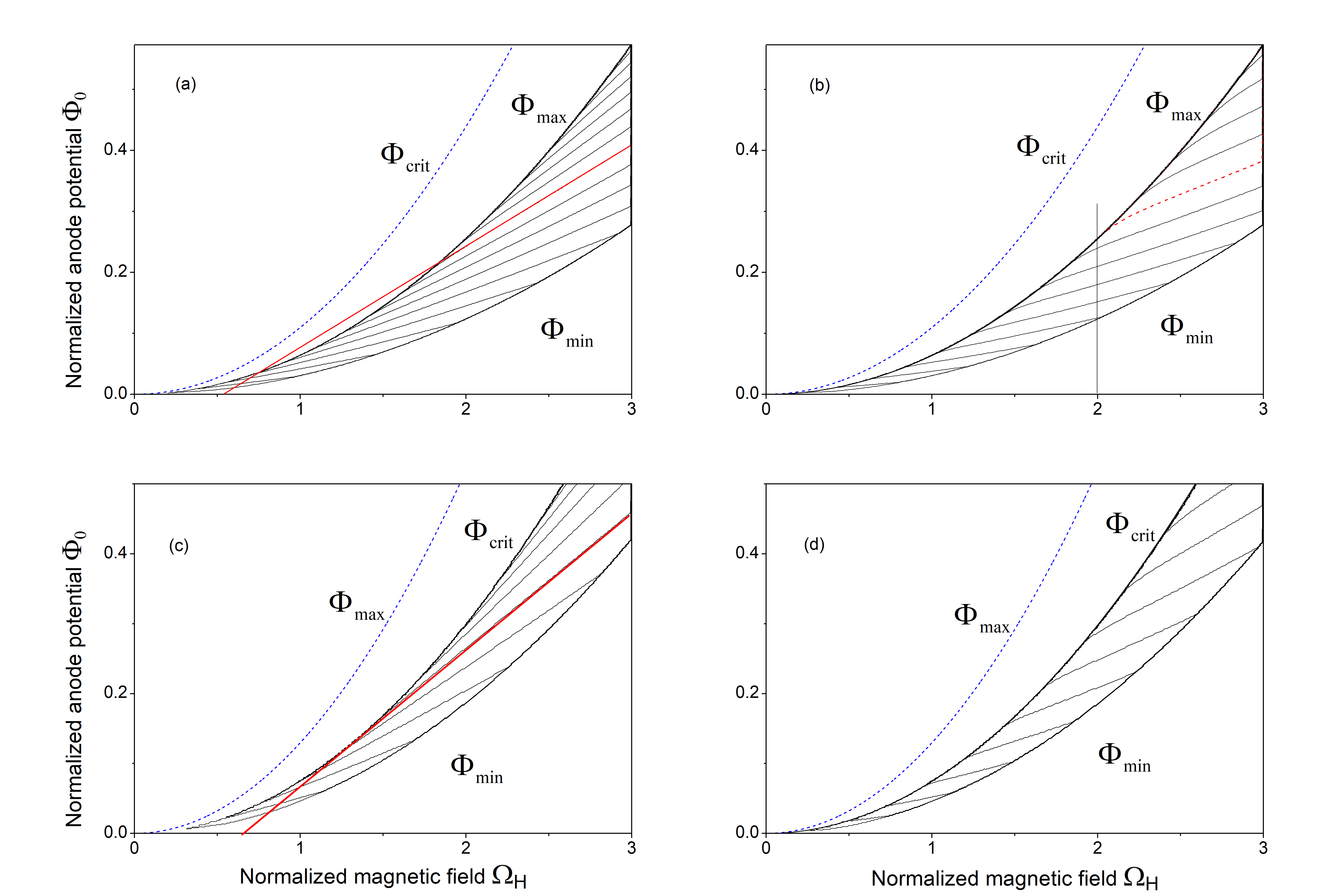
Figure 5: Level lines $\beta={\rm const}$ in the plane $(\Omega_{H},\Phi_{0})$. (a) $\rho_{\rm in}<\rho_{\rm crit}$, (Brillouin flow exists for $\Phi_{\rm min}<\Phi_{0}<\Phi_{\rm max}$. (c) $\rho_{\rm in}>\rho_{\rm crit}$, the existence domain is $\Phi_{\rm min}<\Phi_{0}<\Phi_{\rm HC}$. Thick red line demonstrates that the line $\beta={\rm const}$ is tangent to the curve $\Phi=\Phi_{\rm HC}$ when $\rho_{\rm in}>\rho_{\rm crit}$. Level lines $\nu_{e}={\rm const}$ in the plane $(\Omega_{H},\Phi_{0})$. (b) $\rho_{\rm in}<\rho_{\rm crit}$; (d) $\rho_{\rm in}>\rho_{\rm crit}$. If $\rho_{\rm in}<\rho_{\rm crit}$ [panel(b)], then $\nu=\Omega_{H}/2$ at the line $\Phi_{\rm max}(\Omega_{H})$. As an example, the $\nu=1$ level is indicated by a dashed line.

The condition $\beta={\rm const}$ represented by a straight line is tangent to the curve $\Phi=\Phi_{\rm HC}$ like for a magnetron with a conventional solid axial cathode, only when $\Phi_{\rm HC}$ is inside the permissible interval, as shown in Fig. 5c.

However, if $\rho_{\rm in}<\rho_{\rm crit}$, the outer electron orbit does not touch the anode, as assumed by the conventional BH condition. For this case it seems reasonable to use an equivalent condition

$$\omega=n\omega_{r},$$ (26)

which is applicable whether the outer electron touches the anode or not. Here $\omega$ is the electromagnetic wave frequency, $n$ is the azimuthal index of the magnetron electromagnetic eigenmode, and $\omega_{r}=v_{\varphi}(r_{m})/r_{m}$ is the electron rotation frequency at the outer surface of the Brillouin flow. It is convenient to introduce the dimensionless frequency $\nu=\beta/\rho_{m}$. The condition $\nu={\rm const}$ is satisfied along thin lines in $\Omega_{H}-\Phi_{0}$ plane, depicted in Fig. 5.

Compared to the magnetron, the smooth-bore magnetron with a split cathode has an important additional parameter, the injection radius $r_{\rm in}$. This radius determines the configuration and parameters of the laminar Brillouin flow and the range of magnetic field and anode potential values, for which this flow exists. The conditions

$$\Phi_{0}=\min\{\Phi_{\rm max}(\Omega_{H}),\Phi_{\rm HC}(\Omega_{H})\}$$ (27)

and

$$\omega_{r}(\Phi_{0},\Omega_{H})={\rm const}$$ (28)

play the same role in systems with split cathodes as the HC and BH conditions for the devices with conventional cathodes.

VI discussion

A physical model for the creation of laminar Brillouin flow in the smooth-bore magnetron fed by a split cathode was proposed. It has been shown that the characteristics of the electron flow depends strongly on relations between the radii of the anode $r_{a}$, the central rod $r_{c}$, and the emitting cathode $r_{\rm in}$. Laminar flow cannot form when $r_{\rm in}<1.65r_{c}$. There is a critical value $r_{\rm crit}$ of the radius $r_{\rm in}$, such that when $1.65r_{c}<r_{\rm in}<r_{\rm crit}$, the annular laminar flow does not reach neither the anode nor the rod. If the cathode radius exceeds $r_{\rm crit}$, but is smaller than some value $r_{*}>r_{\rm crit}$, the laminar flow can reach the anode surface. Lastly, laminar flow cannot form when $r_{\rm in}>r_{*}$. Thus, the choice of the emitter radius allows one to obtain different types of electron flow.

The tubular Brillouin flow, whose inner and outer surfaces are separated from metal boundaries, can be formed only in magnetrons with a split cathode. It is well known that this configuration is unstable with respect to the development of the diocotron instability[15]. There is some evidence [8] that the diocotron instability facilitates excitation of electromagnetic oscillations in a cavity magnetron.

Split cathodes offer advantages over conventional cathodes. Explosive emission plasma forms outside the volume of interest and affects only weakly the magnetron operation because the rod anode distance remains unchanged. The proper choice of the radius of the emitting region of the SC allows formation of an electron flow with required characteristics.

- [1] D Price and JN Benford. General scaling of pulse shortening in explosive-emission-driven microwave sources. IEEE TRANSACTIONS ON PLASMA SCIENCE, 26(3):256–262, JUN 1998. International Workshop on High Power Microwave (HPM) Generation and Pulse Shortening, EDINBURGH, SCOTLAND, JUN 10-12, 1997.
- [2] D Price, JS Levine, and JN Benford. Diode plasma effects on the microwave pulse length from relativistic magnetrons. IEEE TRANSACTIONS ON PLASMA SCIENCE, 26(3):348–353, JUN 1998. International Workshop on High Power Microwave (HPM) Generation and Pulse Shortening, EDINBURGH, SCOTLAND, JUN 10-12, 1997.
- [3] M. Siman-Tov, J. G. Leopold, Y. P. Bliokh, and Ya E. Krasik. Periodic bunches produced by electron beam squeezed states in a resonant cavity. PHYSICS OF PLASMAS, 27(8), AUG 2020.
- [4] J. G. Leopold, Ya. E. Krasik, Y. P. Bliokh, and E. Schamiloglu. Producing a magnetized low energy, high electron charge density state using a split cathode. PHYSICS OF PLASMAS, 27(10), OCT 2020.
- [5] G. Liziakin, O. Belozerov, J. G. Leopold, Yu. Bliokh, Y. Hadas, Ya. E. Krasik, and E. Schamiloglu. Experimental research on a split-cathode-fed magnetron driven by long high-voltage pulses. IEEE TRANSACTIONS ON ELECTRON DEVICES, 71(3):2099–2104, MAR 2024.
- [6] Y. Bliokh, Ya. E. Krasik, J. G. Leopold, and E. Schamiloglu. Observation of the diocotron instability in a diode with split cathode. PHYSICS OF PLASMAS, 29(12), DEC 2022.
- [7] Ya. E. Krasik, J. G. Leopold, Y. Hadas, Y. Cao, S. Gleizer, E. Flyat, Y. P. Bliokh, D. Andreev, A. Kuskov, and E. Schamiloglu. An advanced relativistic magnetron operating with a split cathode and separated anode segments. JOURNAL OF APPLIED PHYSICS, 131(2), JAN 14 2022.
- [8] J. G. Leopold, Y. Bliokh, Ya. E. Krasik, A. Kuskov, and E. Schamiloglu. Diocotron and electromagnetic modes in split-cathode fed relativistic smooth bore and six-vane magnetrons. PHYSICS OF PLASMAS, 30(1), JAN 2023.
- [9] Albert W. Hull. The effect of a uniform magnetic field on the motion of electrons between coaxial cylinders. Phys. Rev., 18:31–57, Jul 1921.
- [10] J. C. Slater. Microwave electronics. Rev. Mod. Phys., 18:441–512, Oct 1946.
- [11] O Buneman. Symmetrical states and their breakup. in Crossed Field Microwave Devices, edited by E. Okress, I:209–233, 1961.
- [12] Y. Y. Lau, J. W. Luginsland, K. L. Cartwright, D. H. Simon, W. Tang, B. W. Hoff, and R. M. Gilgenbach. A re-examination of the buneman–hartree condition in a cylindrical smooth-bore relativistic magnetron. Physics of Plasmas, 17(3):033102, 03 2010.
- [13] Léon Brillouin. Theory of the magnetron. i. Phys. Rev., 60:385–396, Sep 1941.
- [14] WE Waters. A theory of magnetron injection guns. IEEE TRANSACTIONS ON ELECTRON DEVICES, 10:226–234, JUL 1963.
- [15] Ronald C Davidson. Physics of nonneutral plasmas. World Scientific Publishing Company, 2001.