Neural Chaos:
A Spectral Stochastic Neural Operator

Abstract

Building surrogate models with uncertainty quantification capabilities is essential for many engineering applications where randomness—such as variability in material properties, boundary conditions, and initial conditions—is unavoidable. Polynomial Chaos Expansion (PCE) is widely recognized as a to-go method for constructing stochastic solutions in both intrusive and non-intrusive ways. Its application becomes challenging, however, with complex or high-dimensional processes, as achieving accuracy requires higher-order polynomials, which can increase computational demands and or the risk of overfitting. Furthermore, PCE requires specialized treatments to manage random variables that are not independent, and these treatments may be problem-dependent or may fail with increasing complexity. In this work, we aim to adopt the same formalism as the spectral expansion used in PCE; however, we replace the classical polynomial basis functions with neural network (NN) basis functions to leverage their expressivity. To achieve this, we propose an algorithm that identifies NN-parameterized basis functions in a purely data-driven manner, without any prior assumptions about the joint distribution of the random variables involved, whether independent or dependent, or about their marginal distributions. The proposed algorithm identifies each NN-parameterized basis function sequentially, ensuring they are orthogonal with respect to the data distribution. The basis functions are constructed directly on the joint stochastic variables without requiring a tensor product structure or assuming independence of the random variables. This approach may offer greater flexibility for complex stochastic models, while simplifying implementation compared to the tensor product structures typically used in PCE to handle random vectors. This is particularly advantageous given the current state of open-source packages, where building and training neural networks can be done with just a few lines of code and extensive community support. We demonstrate the effectiveness of the proposed scheme through several numerical examples of varying complexity and provide comparisons with classical PCE.

Keywords Stochastic Process  $\cdot$ Spectral Representation  $\cdot$ Polynomial Chaos Expansion  $\cdot$ Scientific Machine Learning  $\cdot$ Machine Learning

1 Introduction

Uncertainty quantification (UQ) is a cornerstone of scientific computing, encompassing the identification, propagation, and management of uncertainties throughout the computational modeling process. These uncertainties can arise from various sources, including observational data, modeling assumptions, numerical approximations, and stochastic variability in system inputs. Propagating uncertainty from the stochasticity in input information to the final model predictions is a critical subset of UQ, with significant implications in engineering disciplines. For instance, UQ enables the estimation of confidence intervals for predictions, which is crucial for informed decision-making under uncertainty. It also guides engineers and modelers in designing new experiments or refining models to reduce uncertainties, thereby improving reliability and robustness. These capabilities are vital in high-consequence engineering applications, such as aerospace, nuclear energy, and structural safety, where even small errors in prediction can lead to catastrophic outcomes.

UQ methods can be broadly categorized into two approaches of intrusive and non-intrusive. Intrusive methods require direct modifications to the continuous form of governing equations or their discrete approximations to incorporate uncertainty directly into the computational model. On the other hand, non-intrusive methods do not modify the computational model itself. Instead, they treat the model as a black-box, using techniques like sampling to explore the input space and analyze the resulting outputs. Since intrusive methods require direct access to the governing equations and involve modifying the computational model accordingly, they present significant challenges for problems where the governing equations are unavailable or the computational model is highly complex (e.g., nonlinear finite element methods).

As a result, there is considerable interest in non-intrusive methods, which only require sampling the real physical system, computational model, or legacy codes without making any modifications to them. This flexibility makes non-intrusive methods particularly appealing for practical applications in a plug-and-play manner. Non-intrusive methods may rely on sampling techniques to conduct experiments on the physical system and directly quantify the output prediction uncertainty; or alternatively they may use the samples to build a stochastic surrogate model of the underlying system. The latter approach is often more appealing, as it not only quantifies uncertainty but also provides a differentiable replica of the physical system. This surrogate model can then be leveraged for sensitivity analysis, reliability assessments, and design optimization.

Among the various hypothesis classes of functions used to build stochastic surrogate models, Polynomial Chaos Expansions (PCE) have gained significant attention in engineering applications [hosder2006non, lüthen2021sparse, novak2024physics, sharma2024physics, giovanis2024polynomial]. This is due to their robustness in uncertainty quantification and strong mathematical rigor due to spectral expansion formalism [ghanem2003stochastic, mercer1909xvi], offering a systematic framework for representing stochastic processes and accurately propagating uncertainties in complex systems. However, certain aspects of their mathematical construction can impose limitations. First, PCEs heavily rely on a tensor product structure to simplify statistical moment calculations over a random vector by assuming its marginals are statistically independent. Consequently, when modeling (linearly or nonlinearly) correlated random variables, special treatments, such as transformations or dependency modeling through copulas, are required to account for these correlations effectively. These treatments are problem-specific and may not be effective in general setups [sklar1959fonctions, joe2014dependence, emile1960distributions]. Secondly, PCE requires knowledge of the marginal distributions of the random variables to construct appropriate mutually orthogonal basis functions. This reliance on predefined distributions can limit the PCE applicability when the true distributions are unknown or when the random variables exhibit complex or non-standard distributions. Notably, generalized Polynomial Chaos Expansions (gPCE) [xiu2002wiener] and arbitrary PCE (aPCE) [oladyshkin2012data] can handle arbitrary marginal distributions, provided the random variables are independent. However, this raises concerns regarding the first limitation mentioned: the need to assume independence of random variables to approximate multivariate basis functions as tensor products of univariate ones, where both the independence assumption and the tensor product structure may limit modeling flexibility.

This work introduces Neural Chaos to address these limitations, allowing the retention of all the desirable properties of the spectral expansion formalism while constructing multivariate basis functions in a data-driven manner. These basis functions are designed to operate on the joint distribution of random variables without requiring tensor product decomposition, prior knowledge of marginal distributions, or the independence assumption of the input random variables. Moreover, we establish the connection between the classical spectral expansion, in particular PCEs, for describing stochastic processes with modern operator learning frameworks, in particular Deep Operator Network (DeepONet) [lu2021learning, chen1995universal].

The remainder of this paper is organized as follows. First, we present the spectral stochastic formulation, one of the main building blocks of Neural Chaos, and discuss how it connects to operator learning methods. In section˜2, we provide the details of the Neural Chaos formulation and introduce two algorithms for learning the NN-parametrized basis functions utilized in Neural Chaos. In LABEL:sec:exam, we validate and demonstrate the proposed algorithms using five numerical examples. Finally, we conclude in LABEL:sec:conclusion by summarizing the major findings of this work.

1.1 Spectral Stochastic Methods

Consider the general stochastic partial differential equation given by

$$\mathcal{G}(\bm{x},t,\boldsymbol{\pazocal{X}}(\omega);u(\bm{x},t,\boldsymbol{\pazocal{X}}(\omega)))=f(\bm{x},t,\boldsymbol{\pazocal{X}}(\omega)), \forall\bm{x}\in\mathcal{D}_{x},t\in\mathcal{T},\omega\in\Omega$$ (1)

where $\mathcal{T}\subset\mathbb{R}$, $\mathcal{D}_{x}\subset\mathbb{R}^{3}$, $\mathcal{G}$ is a differential operator, $u(\cdot)$ is the response/solution of the system, $f$ is an external force/source term, and $\boldsymbol{\pazocal{X}}(\omega)\in\mathbb{R}^{d}$ is a $d$-dimensional random vector having sample space $\Omega$.

The classical spectral stochastic approach to solve this system, first introduced by Ghanem and Spanos [ghanem2003stochastic], expands the solution $u(\bm{x},t,\boldsymbol{\pazocal{X}}(\omega))$ as a stochastic process using spectral methods according to the Wiener-Askey polynomial chaos expansion (PCE) [xiu2002wiener] as

$$u(\bm{x},t,\bm{\xi})=\sum_{p=0}^{\infty}\Phi_{p}(\bm{x},t)\Psi_{p}(\bm{\xi})\approx u^{(P)}(\bm{x},t,\bm{\xi})\triangleq\sum_{p=0}^{P}\Phi_{p}(\bm{x},t)\Psi_{p}(\bm{\xi}),$$ (2)

where the random variables $\boldsymbol{\pazocal{X}}(\omega)$ are transformed to standardized space according to $\bm{\xi}=T(\boldsymbol{\pazocal{X}})$ having probability density $p_{\bm{\xi}}(\bm{\xi})$, $\Psi_{p}(\bm{\xi})$ are orthogonal polynomials defined according to the Askey scheme [askey1985some], and $\Phi_{p}(\bm{x},t)$ are deterministic spatio-temporal expansion coefficients that must be determined. Note the random variables, $\bm{\xi}$, are typically considered to be independent such that the multi-variate orthogonal polynomials $\Psi_{p}(\bm{\xi})$ are expressed as a tensor product of univariate orthogonal polynomials $\Psi_{p}(\bm{\xi})=\prod_{m=1}^{d}\psi_{pm}(\xi_{m})$ and the joint distribution can be expressed as the product of the marginal distributions $p_{\bm{\xi}}(\bm{\xi})=\prod_{m=1}^{d}p_{\xi_{m}}(\xi_{m})$. Note also that the expansion in Eq. (2) is truncated to have a total number of terms given by

$$P=\begin{pmatrix}d+n\\ n\end{pmatrix}=\dfrac{(d+n)!}{d!n!},$$ (3)

where $d$ is the dimension of the random variable $\bm{\xi}$ and $n$ is the highest order of the polynomials $\{\psi_{p}\}$.

The expansion coefficients $\Phi_{p}(\bm{x},t)$ can be determined by substituting the expansion in Eq.˜2 into the differential equation in Eq.˜1 and performing a Galerkin projection onto the orthogonal polynomial basis functions $\{g_{p}\}$ as

$$\left\langle\mathcal{G}\left(\bm{x},t,\boldsymbol{\pazocal{X}}(\omega);\sum_{p=0}^{P}\Phi_{p}(\bm{x},t)\Psi_{p}(\bm{\xi})\right),\Psi_{k}\right\rangle=\langle f,\Psi_{k}\rangle,\quad k=0,1,\dots,P.$$ (4)

This defines a coupled set of $(P+1)$ equations that can be solved for $\Phi_{p}(\bm{x},t)$ using classical numerical solvers, e.g., finite elements, by discretizing over the space $\bm{x}$ and time $t$. This class of spectral stochastic methods has been explored in great detail in the literature [ghanem2003stochastic, babuska2004galerkin, xiu2009fast, xiu2010numerical] and has become a benchmark in solving stochastic systems [smith2024uncertainty].

Alternatively, when $u$ is a low-dimensional or scalar-valued quantity of interest (QoI) – e.g., when it is a scalar performance metric/value extracted from the full spatio-temporal solution $u(\bm{x},t)$ – and a set of $N$ sample QoIs are available the coefficients $\Phi_{p}$ can be determined through regression. That is, given a set of $N$ samples of $\bm{\xi}_{i},i=1,\dots,N$ and corresponding QoIs $\bm{u}_{i}$, the coefficients $\Phi_{p}$ can be determined by solving the following ordinary least squares problem [berveiller2006stochastic]

$$\min_{\bm{\Phi}}\sum_{i=1}^{N}\left[\bm{u}_{i}-\bm{u}^{(P)}(\bm{\xi}_{i})\right]^{2}=\min_{\bm{F}}\lVert\bm{U}-\bm{\Phi}^{\intercal}\bm{\Psi}\rVert^{2},$$ (5)

where $\bm{\Phi}=\{\bm{\Phi}_{p}\}$, $\bm{\Psi}=\{\Psi_{pi}\}$, $\bm{U}=\{\bm{u}_{i}\}$, and $\Psi_{pi}$ is the $p$-th basis function evaluated at the $i$-th sample.

This regression-based approach has become increasingly popular in recent years for solving engineering problems in uncertainty quantification. This is because the regression approach is non-intrusive. That it, it does not require the development of custom numerical solvers and allows for surrogate model development in the form of Eq.˜2 from a finite number $N$ of samples obtained by solving Eq.˜1 deterministically at fixed values of $\bm{\xi}_{i},i=1,\dots,N$, often using commercially available numerical solvers. This has led to the rapid growth of advanced regression method using e.g., sparse regression and hyperbolic truncation schemes [blatman2011adaptive], as well as the recognition that PCE can be posed in a purely data-driven sense as a machine learning regression problem [torre2019data]. This is the view that we take in this work.

1.2 The Importance of Orthogonality

The essential element of spectral stochastic methods is that the basis functions $\Psi_{p}(\bm{\xi})$ must be orthogonal with respect to the probability distribution $p_{\bm{\xi}}(\bm{\xi})$. That is,

$$\langle\Psi_{p},\Psi_{k}\rangle\triangleq\int_{\Omega}\Psi_{p}(\bm{\xi})\Psi_{k}(\bm{\xi})p_{\bm{\xi}}(\bm{\xi})d\bm{\xi}=\|\Psi_{p}\|^{2}\delta_{pk}.$$ (6)

Employing orthonormal basis functions, we have $\|\Psi_{p}\|^{2}=1$, where $\|\cdot\|$ denotes the norm associated with the specified inner product. This enables the Galerkin projection in Eq.˜4, ensuring that the error is orthogonal to the function space spanned by $\Psi_{p}(\bm{\xi})$. Moreover, this orthogonality yields convenient properties of the PCE in Eq. (2) for uncertainty quantification. Specifically, moments of the solution $u(\bm{x},t,\bm{\xi})$ can be estimated directly from the coefficients $\Phi_{p}(\bm{x},t)$ where the mean function is given by $\Phi_{0}(\bm{x},t)$ and the second moment is given by

$$\mathbb{E}_{\bm{\xi}}[{{u^{2}}(\bm{x},t,\bm{\xi})}] =\int{\left[{\sum\limits_{p=0}^{P}{{\Phi_{p}(\bm{x},t)}{\Psi_{p}}\left(\bm{\xi}\right)}}\right]}^{2}p_{\bm{\xi}}(\bm{\xi})\;\mathrm{d}\bm{\xi}=\sum\limits_{p=0}^{P}\sum\limits_{k=0}^{P}\Phi_{p}(\bm{x},t)\Phi_{k}(\bm{x},t)\int{\Psi_{p}}\left(\bm{\xi}\right){\Psi_{k}}\left(\bm{\xi}\right)p_{\bm{\xi}}(\bm{\xi})\;\mathrm{d}\bm{\xi}$$ (7)

$$=\sum\limits_{p=0}^{P}{\Phi_{p}^{2}(\bm{x},t)}{\int{\Psi_{p}^{2}}\left(\bm{\xi}\right)}p_{\bm{\xi}}(\bm{\xi})\;\mathrm{d}\bm{\xi}=\sum\limits_{p=0}^{P}{\Phi_{p}^{2}(\bm{x},t)}\|g_{p}\|^{2}=\sum\limits_{p=0}^{P}{\Phi_{p}^{2}(\bm{x},t)}.$$

Additionally, higher-order moments [novak2022distribution], fractional moments [novak2024fractional], and sensitivity indices [sudret2008global, novak2022distribution] can be derived directly from the coefficients. This makes the PCE very powerful for uncertainty quantification.

1.3 Challenges of Spectral Stochastic Methods

In spectral stochastic methods, orthogonality is guaranteed by selecting the basis functions $\Psi_{p}(\bm{\xi})$ according to the Askey scheme of orthogonal polynomials. This is the primary strength of spectral stochastic methods, but also leads to some drawbacks and associated challenges. Polynomial functions, while inherently smooth and differentiable, are not optimally expressive and may fail to produce representations that generalize well. The consequence of this is that PCE methods may require high-order polynomial terms to fit non-linear functions, but these high-order polynomials lead to instabilities (e.g., Runge’s phenomenon, bad conditioned design matrix, etc.) that result in over-fitting [kontolati2023influence]. Hence, there is a trade-off between generalization (requiring low-order polynomials) and expressivity (requiring high-order polynomials).

A related issue is the polynomial growth of the number of terms in a PC expansion; $P$ in Eq.˜3 scales as $O(n^{d})$ for fixed dimensions $d$ and as $O(d^{n})$ for a fixed polynomial order $n$. This results in an explosion of the number of coefficients that need to be solved for. For stochastic Galerkin methods, the consequence is a very large system of equations that must be solved using numerical methods – effectively an explosion in the number of degrees of freedom in the numerical model. As a result, spectral stochastic methods typical employ only low-order polynomials and struggle with strongly non-linear problems. For regression methods, again the number of coefficients grows extremely large, which either necessitates very large training data sets (that come at high computational expense) or requires sophisticated sparse regression such as methods like Least Angle Regression [blatman2011adaptive], Bayesian compressive sensing [hampton2015compressive, tsilifis2019compressive], partial least squares [papaioannou2019pls], and many other methods have become standard practice. A comprehensive review can be found in [lüthen2021sparse]. Even with these methods, regression-based PCE may require the determination of hundreds to thousands of coefficients while balancing the trade-off between generalization and over-fitting [kontolati2023influence].

The PCE is also generally constrained by the class of polynomials that are available for the analytical construction of the polynomial chaos expansion in Eq. (2). These classes constrain the types on uncertainties that can be included to those with common and well-known distributions – e.g. Gaussian, uniform – and independent marginal distributions resulting in tensor product basis construction. For distributions that do not follow the Askey scheme or involve dependent variables, analytical spectral expansions are scarce and typically valid only under special conditions [rahman2018polynomial]. Recent advances do allow for the construction of polynomial chaos expansions for random variables with aribitrary distributions, termed arbitrary PCE [soize2004physical, oladyshkin2012data]. These approaches build orthogonal polynomial basis functions with coefficients that can be solved directly from statistical moments estimated from the given dataset. These methods have been shown to perform well in a data-driven setting where the form of the distribution $p_{\bm{\xi}}(\bm{\xi})$ is not known analytically [soize2004physical, oladyshkin2012data].

A final, and important drawback of regression-based PCE is usually used to define a surrogate model for a low-dimensional (often scalar-valued) quantity of interest derived from the solution $u$. Regression-based PCE methods generally cannot learn the coefficient functions $\Phi_{p}(\bm{x},t)$ needed to express the full spatio-temporal solution $u(\bm{x},t)$. Rather, they generally learn scalar coefficients $\Phi_{p}$ that, as previously mentioned, can be used to build surrogate models for scalar response quantities of interest derived from the full solution $u(\bm{x},t)$. This severely limits the PCE as a modeling framework for operator learning, which is of interest in this work and is briefly discussed next.

1.4 PCE for Operator Learning

A few recent works have begun to explore PCE in a context that can be considered operator learning – although these methods are not formally stated or presented as operator learning methods. The formal problem statement for operator learning will be presented in the following section. For the present purposes, we will state the (deterministic) operator learning problem informally as any method that attempts to learn the operator $\mathcal{G}(\cdot)$ through a functional $\mathcal{G}_{\theta}(\cdot)$ with parameters $\theta$ such that $u(\bm{x},t,\bm{\xi})\approx\mathcal{G}_{\theta}(\bm{x},t,\bm{\xi},f)$.

To solve this operator learning problem, Kontolati et al. [kontolati2022manifold, kontolati2022survey] developed the manifold PCE (mPCE) method that can be view as an operator learning method. The mPCE method is a regression-based approach in which realizations of, for example, $f(\bm{x},t,\bm{\xi}_{i}),i=1,\dots,N$ and corresponding solutions $u(\bm{x},t,\bm{\xi}_{i})$ are projected onto a low-dimensional manifold. A PCE model is then fit between the projected low-dimensional input and the corresponding low-dimensional solution. For any new input, $f(\bm{x},t,\bm{\xi}^{*})$ is projected onto the manifold, the low-dimensional solution is predicted with the PCE model, and the low-dimensional solution is then lifted back to reconstruct the approximate output function $\tilde{u}(\bm{x},t,\bm{\xi}^{*})$ by inverting the solution projection operator. This procedure is generalizable and amenable to various forms of dimension reduction ranging from linear methods such as principal component analysis to nonlinear manifold learning methods such as diffusion maps and autoencoders. Kontolati et al. [kontolati2022survey] performed a comprehensive study of the mPCE method for different classes of unsupervised dimension reduction methods and Kontolati et al. [kontolati2023influence] then compared this approach with neural network-based operator learning using the deep operator network (DeepONet).

Very recently, Novak et al. [novak2024physics] and Sharma et al. [sharma2024physics] introduced the physics-constrained polynomial chaos expansion (PC²). This approach, which introduces physics-informed learning in the context of PCE, defines orthogonal polynomial basis functions over the spatial and temporal variables such that the coefficient functions $\Phi_{i}(\bm{x},t)$ are, themselves, expressed through a polynomial chaos expansion. Doing so allows the least squares solution to be constrained (by physical constraints, i.e., PDEs, or arbitrary constraints such as inequalities), which is the objective of these works. But, by formulating the coefficient functions in this way, the authors also extend the classical regression-based PCE to an operator learning setting where the full spatial-temporal solution can be predicted.

2 Formulation

In this section, we break from the classical spectral stochastic methods by formulating the general operator learning problem for stochastic problems and demonstrating how this operator learning problem can be solved using a new class of spectral stochastic neural operators. Rather than employing orthogonal polynomials, these spectral stochastic neural operators learn a dictionary of orthogonal functions, constructed as neural networks, that serve as a compact basis for the spectral expansion. Importantly, these learned basis functions maintain the orthogonality properties introduced in Section 1.2, which endows them with the beneficial properties of existing spectral stochastic methods (e.g., easier moment estimation). They can be learned for arbitrary distributions and are not constrained by a tensor product structure meaning they can uphold orthogonality to joint distributions with arbitrary dependence structure. However, if a tensor product serves as a strong inductive bias or is computationally justified, one can still use the proposed scheme while parametrizing a subset or all basis functions in a tensor product fashion [cho2022separable].

2.1 Operator Learning Between Random Function Spaces

Let’s begin by framing the stochastic operator learning problem in the classic setting of Chen and Chen [chen1995universal] adopted most notably in the Deep Operator Network (DeepONet) [lu2021learning] by considering that we aim to approximate the solution operator for a given input at a specific point $\bm{y}=\{\bm{x},t,\bm{\xi}\}$ conditioned on the input function $g$ (e.g., operator source term) where $\bm{y}$ concatenates the spatial and temporal locations of the prediction with the random vector $\bm{\xi}$ and $\bm{g}$ concatenates the parts of the PDE operator that we have access to as input function information. In this setting, the neural operator can be formulated as

$$\mathcal{G}(g)(\bm{y}) \approx\sum_{s=1}^{S}\underbrace{\sum_{i=1}^{n}\bar{\beta}_{i}^{s}\sigma\left(\sum_{j=1}^{m}\hat{\beta}_{ij}^{s}g_{j}+\tilde{\beta}_{i}^{s}\right)}_{\bar{\Phi}_{s}(\bm{g};\beta_{s})}\underbrace{\sigma(\bar{\theta}_{s}\bm{y}+\tilde{\theta}_{s})}_{\bar{\Psi}_{s}(\bm{y};\theta_{s})}$$ (8)

$$=\sum_{s=1}^{S}\bar{\Phi}_{s}(\bm{g};\beta_{s})\bar{\Psi}_{s}(\bm{y};\theta_{s}),$$

where $\sigma$ is a nonlinear activation function (e.g., tanh), $\bar{\beta}_{i}^{s}$, $\hat{\beta}_{i}^{s}$, $\tilde{\beta}_{i}^{s}$, $\bar{\theta}_{i}^{s}$, $\tilde{\theta}_{i}^{s}$, are tunable parameters whose their collections are denoted by $\beta_{s}=\{\bar{\beta}_{i}^{s},\hat{\beta}_{i}^{s},\tilde{\beta}_{i}^{s}\}$ and $\theta_{s}=\{\bar{\theta}_{i}^{s},\tilde{\theta}_{i}^{s}\}$, respectively. According to Eq.˜8, $\bar{\Phi}_{s}(\bm{g};\beta_{s})$ defines the branch network and $\bar{\Psi}_{s}(\bm{y};\theta_{s})$ is a global trunk network that spans the output over the combined spatio-temporal and stochastic spaces. We refer to this naive implementation as the Stochastic DeepONet.

The Stochastic DeepONet in Eq.˜8 is a straightforward extension of the DeepONet with predictive ability for stochastic problems at arbitrary $\bm{x}$, $t$, and $\bm{\xi}$. However, it lacks the properties of the spectral expansion that, as argued above, are desirable for stochastic problems. In particular, the basis functions $\bar{\Psi}_{s}(\bm{y};\theta_{s})$ should be orthogonal with respect to $p_{\bm{\xi}}(\bm{\xi})$. According to the formulation in Eq.˜8, this can only be achieved by integrating the conditions in Eq.˜6 into the loss function. Although this is perhaps possible, it may require a separable tensor product architecture [cho2022separable, mandl2024separable, yu2024separable] (which assumes independent random variables). This approach can pose significant computational challenges for optimization, particularly when evaluating and enforcing all orthogonality integrals during each training iteration. This cost and the associated challenges may compound rapidly as the number of dimensions, $d$, increases.

The function $\bar{\Psi}_{s}(\bm{y})$ can be universally approximated as $\bar{\Psi}_{s}(\bm{y})=\sum_{q=1}^{\infty}\hat{\Phi}_{sq}(\bm{x},t)\hat{\Psi}_{sq}(\bm{\xi})$, which follows the spectral stochastic expansion in Eq. (2). Substituting this into Eq.˜8, we obtain:

$$\mathcal{G}(g)(\bm{y}) \approx\sum_{s=1}^{S}\bar{\Phi}_{s}(\bm{g})\sum_{q=1}^{\infty}\hat{\Phi}_{sq}(\bm{x},t)\hat{\Psi}_{sq}(\bm{\xi})$$ (9)

$$=\sum_{q=1}^{\infty}\sum_{s=1}^{S}\bar{\Phi}_{s}(\bm{g})\hat{\Phi}_{sq}(\bm{x},t)\hat{\Psi}_{sq}(\bm{\xi})$$

$$=\sum_{p=1}^{\infty}\underbrace{\bar{\Phi}_{p}(\bm{g})\hat{\Phi}_{p}(\bm{x},t)}_{{\Phi}_{p}(\bm{g},\bm{x},t)}{\Psi}_{p}(\bm{\xi})$$

$$=\sum_{p=1}^{\infty}\Phi_{p}(\bm{g},\bm{x},t){\Psi}_{p}(\bm{\xi})$$

$$\approx\sum_{p=1}^{P}\Phi_{p}(\bm{g},\bm{x},t){\Psi}_{p}(\bm{\xi}).$$

The proposed formulation in Eq.˜9, which we refer to as the Spectral Stochastic Neural Operator (or Neural Chaos in homage to the aforementioned polynomial chaos), differs subtly in construction from the Stochastic DeepONet but now clearly takes the desirable form of a spectral expansion (see Eq. (2)) if we can ensure that $\bar{\Psi}_{p}(\bm{\xi};\beta_{p})$ satisfy the orthogonality conditions in Eq.˜6. This is the primary challenge addressed herein.

Remark 2.1.

In this work, we lump all sources of uncertainty, such as errors regarding boundary conditions, initial conditions, domain boundary, PDE operator, measurements, etc., into random variables $\bm{\xi}$, while in some applications, it might be important to identify and separate different sources of uncertainty. We leave such an extension as a promising direction for future studies.

2.2 Building Spectral Stochastic Neural Network Basis Functions

A naive way to build the Spectral Stochastic Neural Operator would, again, be to enforce orthogonality through the loss function. But this may run into the same huge computational challenges discussed above. Instead, we propose an iterative algorithm that learns the stochastic basis functions $g_{p}(\bm{\xi};\beta_{p})$ and the associated spatio-temporal coefficients $f_{p}(\bm{x};\theta_{p})$ together as a sequence of neural networks that are (approximately) orthogonal by construction. This proposed architecture is presented in Figure 1.

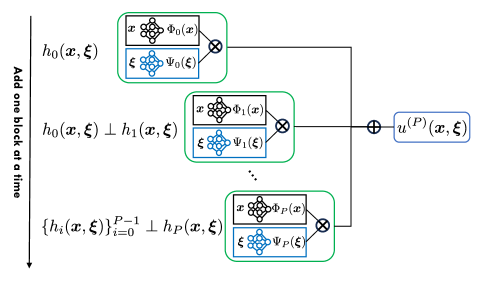
Figure 1: Neural Chaos architecture, which mirrors the structure of a spectral expansion. Spectral terms are added one by one such that each new term is orthogonal to the previous ones. Each spectral term has a multiplicative structure with $h_{i}(\bm{x},\bm{\xi})=\Phi_{i}(\bm{x})\Psi_{i}(\bm{\xi})$ comprising deterministic and stochastic basis functions, each parameterized by a neural network.

To construct orthogonal stochastic basis functions using neural networks (i.e., without leveraging a class of predetermined orthogonal functions such as orthogonal polynomials), we follow the residual-based approach initially proposed in [bahmani2024resolution] in the context of neural operator learning, which we use here for stochastic processes.

Lemma 2.2.

The truncated residual $r^{(p)}(\bm{x},\bm{\xi})=u(\bm{x},\bm{\xi})-u^{(p)}(\bm{x},\bm{\xi})$ of the spectral expansion series, as described by Equation 2, is itself a random process that is orthogonal to the series basis functions $\Psi_{i}$ if these bases are orthonormal in $L^{2}(p(\bm{\xi}))$, i.e., mutually orthogonal and unit norm.

Proof.

We simply need to show that the inner product of the residual with any stochastic basis $\Psi_{i}(\bm{\xi})$ is zero:

$$\langle r^{(p)},\Psi_{i}\rangle =\mathbb{E}_{\bm{\xi}}\left[\Psi_{i}(\bm{\xi})\left(u(\bm{x},\bm{\xi})-u^{(p)}(\bm{x},\bm{\xi})\right)\right]$$ (10)

$$=\mathbb{E}_{\bm{\xi}}\left[\Psi_{i}(\bm{\xi})\left(u(\bm{x},\bm{\xi})-\sum_{j=0}^{p}\Phi_{j}(\bm{x})\psi_{j}(\bm{\xi})\right)\right]$$ (11)

$$=\mathbb{E}_{\bm{\xi}}\left[\Psi_{i}(\bm{\xi})u(\bm{x},\bm{\xi})\right]-\sum_{j=0}^{p}\Phi_{j}(\bm{x})\mathbb{E}_{\bm{\xi}}\left[\Psi_{i}(\bm{\xi})\Psi_{j}(\bm{\xi})\right]$$ (12)

$$=\Phi_{i}(\bm{x})-\Phi_{i}(\bm{x})\|\Psi_{i}(\bm{\xi})\|^{2}_{L^{2}(p(\bm{\xi}))}=0.$$ (13)

∎

Lemma 2.3.

For any multiplicative composition of a stochastic function $\bar{\Psi}(\bm{\xi})\neq 0$ and a deterministic function $\bar{\Phi}(\bm{x})\neq 0$ that reduces the truncated residual, the stochastic function cannot belong to the subspace spanned by the stochastic basis functions used in the truncation series, i.e.,

$$\|r^{(p)}(\bm{x},\bm{\xi})-\bar{\Phi}(\bm{x})\bar{\Psi}(\bm{\xi})\|^{2}<\|r^{(p)}(\bm{x},\bm{\xi})\|^{2}\implies\bar{\Psi}(\bm{\xi})\notin\text{span}\{\Psi_{j}(\bm{\xi})\}_{j=1}^{p}.$$ (14)

Proof.

By contradiction, we need to show that if $\bar{\Psi}(\bm{\xi})$ belongs to the subspace of basis functions, then there is no way to reduce the residual. If $\bar{\Psi}(\bm{\xi})$ belongs to the subspace, it can be spanned linearly by the basis functions, i.e., $\bar{\Psi}(\bm{\xi})=\sum_{j=1}^{p}\alpha_{j}\Psi_{j}(\bm{\xi})$:

$$\|r^{(p)}(\bm{x},\bm{\xi})-\bar{\Phi}(\bm{x})\bar{\Psi}(\bm{\xi})\|^{2} =\mathbb{E}_{\bm{\xi}}\left[\left(r^{(p)}(\bm{x},\bm{\xi})-\bar{\Phi}(\bm{x})\bar{\Psi}(\bm{\xi})\right)^{2}\right]$$ (15)

$$=\|r^{(p)}\|^{2}+\underbrace{\bar{\Phi}^{2}(\bm{x})\|\bar{\Psi}(\bm{\xi})\|^{2}}_{\geq 0}-2\bar{\Phi}(\bm{x})\underbrace{\mathbb{E}_{\bm{\xi}}\left[r^{(p)}(\bm{x},\bm{\xi})\bar{\Psi}(\bm{\xi}))\right]}_{=0(\text{ orthogonality})}$$ (16)

$$\geq\|r^{(p)}\|^{2}.$$ (17)

∎

Algorithm 1 Continuous Spectral Stochastic Dictionary Learning

1:Input:

2:$\mathcal{D}_{u}=\left\{\mathcal{D}_{u}^{(i)}\right\}_{i=1}^{N},\mathcal{D}_{u}^{(i)}=\left(\bm{\xi}^{(i)},\left\{\bm{x}^{(i,j)},u^{(i,j)}\right\}_{j=1}^{M}\right)$ $\triangleright$ $N$ realizations of the stochastic process $u(\bm{x},\bm{\xi})$

3:$0<\text{Tol.}\ll 1$ $\triangleright$ A small tolerance of target accuracy

4:Output: $P,\Phi_{0}(\cdot;\bm{\theta}_{0}),\left\{\Phi_{p}(\cdot;\bm{\theta}_{p}),\Psi_{p}(\cdot;\bm{\beta}_{p})\right\}_{p=1}^{P}$ $\triangleright$ A set of $2P+1$ parameterized basis functions

5:$p\leftarrow 0$

6:$\bm{\theta}_{0}={\text{argmin}}\ \underset{(\bm{x},\bm{\xi})\sim\mathcal{D}_{u}}{\mathbb{E}}\left\|u(\bm{x},\bm{\xi})-\Phi_{0}(\bm{x};\bm{\theta}_{0})\right\|_{2}^{2}$

7:$r(\bm{x},\bm{\xi})=u(\bm{x},\bm{\xi})-\Phi_{0}(\bm{x};\bm{\theta}_{0})$

8:while $\mathbb{E}_{\bm{x},\bm{\xi}}[r^{2}(\bm{x},\bm{\xi})]\geq\text{Tol.}$ do

9:  $p\leftarrow p+1$

10:  Randomly initialize two new neural networks $\Phi_{p}(\bm{x};\bm{\theta}_{p})$, $\Psi_{p}(\bm{\xi};\bm{\beta}_{p})$

11:  $\bm{\theta}_{p},\bm{\beta}_{p}={\text{argmin}}\ \underset{(\bm{x},\bm{\xi})\sim\mathcal{D}_{u}}{\mathbb{E}}\left\|r(\bm{x},\bm{\xi})-\Phi_{p}(\bm{x};\bm{\theta}_{p})\Psi_{p}(\bm{\xi};\bm{\beta}_{p})\right\|_{2}^{2}$

12:  $r(\bm{x},\bm{\xi})\leftarrow r(\bm{x},\bm{\xi})-\Phi_{p}(\bm{x};\bm{\theta}_{p})\Psi_{p}(\bm{\xi};\bm{\beta}_{p})$

13:end while

Based on these two lemmas, we propose an algorithm that learns the $p$-th term in the spectral expansion by finding the unknown functions $\Phi_{p}(\bm{x};\bm{\theta}_{p})$ and $\Psi_{p}(\bm{\xi};\bm{\beta}_{p})$ that best factorize the stochastic residual field $r^{(p-1)}(\bm{x},\bm{\xi})$ in a multiplicative way. The neural network parameters $\bm{\theta}_{p}$ and $\bm{\beta}_{p}$ are optimized using gradient descent to minimize the expected error across the realizations of the random process. Based on Lemma 2.3, if the residual decays, we can conclude that the newly extended basis function introduces a new function that does not belong to the subspace spanned by the previous basis functions. We call this method “continuous” spectral stochastic dictionary learning, as outlined in Algorithm 1. Note that, similar to PCE-based methods, the zero-th term sets $\Psi_{0}(\bm{\xi})=1$, and accordingly, the deterministic basis function aims to capture the mean field across the realizations (see Line 6 in Algorithm 1).

Learning the basis functions in this way may introduce some challenges during optimization, particularly in Line 11, where an identifiability issue arises. Specifically, one can arbitrarily scale up one of the basis functions and scale down the other by the same factor, while the loss function remains unchanged. Ideas involving alternating optimization and rescaling after each iteration, as proposed in [bahmani2024resolution], can be leveraged to mitigate these issues. However, along these lines, we propose a more robust algorithm as follows: By leveraging the bilinearity of each spectral term, if one of the functions is fixed, the other can be found analytically at the function level, regardless of the chosen parameterization. In other words, this is the optimal solution, independent of how the function has been parameterized via polynomials, neural networks, etc.

Lemma 2.4.

For the fixed $\Psi_{p}(\bm{\xi})$, the optimal $\Phi_{p}(\bm{x})$ has a closed form solution as follows:

$$\underset{\Phi_{p}}{\text{argmin}}\ \mathbb{E}_{\bm{\xi}}[(\Phi_{p}(\bm{x})\Psi_{p}(\bm{\xi})-r(\bm{x},\bm{\xi}))^{2}] =\underset{\Phi_{p}}{\text{argmin}}\ \Phi_{p}^{2}(\bm{x})\mathbb{E}_{\bm{\xi}}[\Psi_{p}^{2}(\bm{\xi})]-2\Phi_{p}(\bm{x})\mathbb{E}_{\bm{\xi}}[\Psi_{p}(\bm{\xi})r(\bm{x},\bm{\xi})]+\mathbb{E}_{\bm{\xi}}[r^{2}(\bm{x},\bm{\xi})]$$ (18)

$$=\underset{\Phi_{p}}{\text{argmin}}\ \Phi_{p}^{2}(\bm{x})\mathbb{E}_{\bm{\xi}}[\Psi_{p}^{2}(\bm{\xi})]-2\Phi_{p}(\bm{x})\mathbb{E}_{\bm{\xi}}[\Psi_{p}(\bm{\xi})r(\bm{x},\bm{\xi})]$$ (19)

$$=\frac{\mathbb{E}_{\bm{\xi}}[\Psi_{p}(\bm{\xi})r(\bm{x},\bm{\xi})]}{\mathbb{E}_{\bm{\xi}}[\Psi_{p}^{2}(\bm{\xi})]}.$$ (20)

Lemma 2.5.

For the fixed $\Phi_{p}(\bm{x})$, the optimal $\Psi_{p}(\bm{\xi})$ has a closed form solution as follows:

$$\underset{\Psi_{p}}{\text{argmin}}\ \mathbb{E}_{\bm{x}}[(\Phi_{p}(\bm{x})\Psi_{p}(\bm{\xi})-r(\bm{x},\bm{\xi}))^{2}] =\underset{\Psi_{p}}{\text{argmin}}\ \Psi_{p}^{2}(\bm{\xi})\mathbb{E}_{\bm{x}}[\Phi_{p}^{2}(\bm{x})]-2\Phi_{p}(\bm{x})\mathbb{E}_{\bm{x}}[\Psi_{p}(\bm{\xi})r(\bm{x},\bm{\xi})]+\mathbb{E}_{\bm{x}}[r^{2}(\bm{x},\bm{\xi})]$$ (21)

$$=\underset{\Psi_{p}}{\text{argmin}}\ \Psi_{p}^{2}(\bm{\xi})\mathbb{E}_{\bm{x}}[\Phi_{p}^{2}(\bm{x})]-2\Psi_{p}(\bm{\xi})\mathbb{E}_{\bm{x}}[\Phi_{p}(\bm{x})r(\bm{x},\bm{\xi})]$$ (22)

$$=\frac{\mathbb{E}_{\bm{x}}[\Phi_{p}(\bm{x})r(\bm{x},\bm{\xi})]}{\mathbb{E}_{\bm{x}}[\Phi_{p}^{2}(\bm{x})]}.$$ (23)

Based on these lemmas, we can first find the optimal basis vectors in a fully discrete manner, and then, in parallel, learn continuous versions of these bases that map the domain of the functions to the identified images via parameterization with neural networks. For example, $\Psi_{p}(\bm{\xi};\bm{\beta}_{p}):\bm{\xi}\to\Psi_{p}(\bm{\xi})$. We call this method “discrete-continuous” spectral stochastic dictionary learning, as outlined in Algorithm 2. The key difference between this algorithm and the previous one lies in Line 11, where we introduce the Closest Multiplicative Decomposition (CMD) iterations, as outlined in Algorithm 3. This provides a practical use case for deriving the closed-form solution for stochastic and deterministic functions, with one of them assumed to be fixed. Note that at the end of each CMD step, we normalize the stochastic basis to have unit norm by appropriately scaling the stochastic and deterministic basis vectors. In this way, the magnitude of the deterministic basis reflects the importance of their corresponding stochastic basis in the overall spectral expansion for approximating the random process under study.

Algorithm 2 Discrete-Continuous Spectral Stochastic Dictionary Learning

1:Input:

2:$\mathcal{D}_{u}=\left\{\mathcal{D}_{u}^{(i)}\right\}_{i=1}^{N},\mathcal{D}_{u}^{(i)}=\left(\bm{\xi}^{(i)},\left\{\bm{x}^{(i,j)},u^{(i,j)}\right\}_{j=1}^{M}\right)$ $\triangleright$ $N$ realizations of the stochastic process $u(\bm{x},\bm{\xi})$

3:$0<\text{Tol.}\ll 1$ $\triangleright$ A small tolerance of target accuracy

4:Output: $P,\Phi_{0},\left\{\Phi_{p},\Psi_{p}\right\}_{p=1}^{P}$ $\triangleright$ A set of $2P+1$ basis vectors

5:$p\leftarrow 0$

6:${\Phi_{0}}_{j}=\mathbb{E}_{i}[u^{(i,j})]$ $\triangleright$ For all $1\leq j\leq M$

7:$r^{(i,j)}=u^{(i,j)}-{\Phi_{0}}_{j}$ $\triangleright$ For all $1\leq j\leq M$ and $1\leq i\leq N$

8:while $\mathbb{E}_{i,j}[||r^{(i,j)}||_{2}^{2}]\geq\text{Tol.}$ do

9:  $\mathcal{D}_{r}=\left\{\mathcal{D}_{r}^{(i)}\right\}_{i=1}^{N},\mathcal{D}_{r}^{(i)}=\left(\bm{\xi}^{(i)},\left\{\bm{x}^{(i,j)},r^{(i,j)}\right\}_{j=1}^{M}\right)$

10:  $p\leftarrow p+1$

11:  $\Phi_{p},\Psi_{p}\leftarrow\text{CMD}(\mathcal{D}_{r})$ $\triangleright$ See Algorithm 3

12:  $r^{(i,j)}\leftarrow r^{(i,j)}-{\Phi_{p}}_{j}{\Psi_{p}}_{i}$ $\triangleright$ For all $1\leq j\leq M$ and $1\leq i\leq N$

13:end while

Algorithm 3 Closest Multiplicative Decomposition

1:Input:

2:$\mathcal{D}_{r}=\left\{\mathcal{D}_{r}^{(i)}\right\}_{i=1}^{N},\mathcal{D}_{r}^{(i)}=\left(\bm{\xi}^{(i)},\left\{\bm{x}^{(i,j)},r^{(i,j)}\right\}_{j=1}^{M}\right)$ $\triangleright$ $N$ realizations of the stochastic process $r(\bm{x},\bm{\xi})$

3:$0<\text{Tol.}\ll 1$ $\triangleright$ A small tolerance of target accuracy

4:Output: $\Phi(\bm{x}),\Psi(\bm{\xi})$ $\triangleright$ Such that $r(\bm{x},\bm{\xi})\approx\Phi(\bm{x})\Psi(\bm{\xi})$

5:$\Psi_{i}=1$ $\triangleright$ Initialize to ones for $1\leq i\leq N$

6:while Not Converged do $\triangleright$ Based on changes in $\Psi(\bm{\xi})$

7:  $\Phi_{j}=\mathbb{E}_{i}[\Psi_{i}r^{(i,j)}]/\|\Psi\|_{L^{2}(p(\bm{\xi}))}$ $\triangleright$ For all $1\leq j\leq M$

8:  $\Psi_{i}=\mathbb{E}_{j}[\Phi_{j}r^{(i,j)}]/\|\Phi\|_{2}^{2}$

9:end while

A useful property of spectral expansion with orthogonal stochastic basis functions is the ability to estimate the variance analytically, without the need for Monte Carlo estimation. One can easily show that if $\Psi_{i}(\bm{\xi})$ are orthogonal, the variance of the truncated approximation $u^{(p)}$ can be calculated as follows:

$$\mathbb{V}_{\bm{\xi}}[u(\bm{x},\bm{\xi})]\approx\mathbb{V}_{\bm{\xi}}[u^{(p)}(\bm{x},\bm{\xi})]=\sum_{i=1}^{P}\Phi_{i}^{2}(\bm{x})\mathbb{E}_{\bm{\xi}}[\Psi_{i}^{2}(\bm{\xi})].$$ (24)

If the stochastic basis functions are normalized, this equation simplifies to a summation over only the deterministic basis functions. We use this method of variance estimation through the identified basis functions as a sanity check to indirectly assess how well they satisfy orthogonality. If their orthogonality is poor, the variance estimated this way will deviate significantly from the true variance. Recall that the mean of the random process is equal to the zeroth-order term $\Phi_{0}(\bm{x})$, i.e.,

$$\mathbb{E}_{\bm{\xi}}[u(\bm{x},\bm{\xi})]\approx\mathbb{E}_{\bm{\xi}}[u^{(p)}(\bm{x},\bm{\xi})]=\Phi_{0}(\bm{x}).$$ (25)