SFTs: a scalable data-analysis framework for long-duration gravitational-wave signals

Abstract

We introduce a framework based on Short-time Fourier Transforms (SFTs) to analyze long-duration gravitational wave signals from compact binaries. Targeted systems include binary neutron stars observed by third-generation ground-based detectors and massive black-hole binaries observed by the LISA space mission. In short, ours is an extremely fast, scalable, and parallelizable implementation of the gravitational-wave inner product, a core operation of gravitational-wave matched filtering. By operating on disjoint data segments, SFTs allow for efficient handling of noise non-stationarities, data gaps, and detector-induced signal modulations. We present a pilot application to early warning problems in both ground- and space-based next-generation detectors. Overall, SFTs reduce the computing cost of evaluating an inner product by three to five orders of magnitude, depending on the specific application, with respect to a standard approach. We release public tools to operate using the SFT framework, including a vectorized and hardware-accelerated re-implementation of a time-domain waveform. The inner product is the key building block of all gravitational-wave data treatments; by speeding up this low-level element so massively, SFTs provide an extremely promising solution for current and future gravitational-wave data-analysis problems.

I Introduction

The detection of gravitational-wave signals (GWs) from compact object coalescences (CBCs), such as binary black holes (BBHs) or neutron stars (BNS) is now routine [1, 2, 3, 4]. As observed by the current network of ground-based detectors (LIGO [5], Virgo [6], and KAGRA [7]), these signals sweep the audible band of the GW spectrum with durations ranging from a fraction of a second for BBHs to up to a few minutes for BNSs.

The duration of a GW signal is a function of both the intrinsic properties of the system —notably its chirp mass— and the minimum sensitive frequency of the detector [8]. While LIGO/Virgo/KAGRA are sensitive to frequencies $\gtrsim$10\text{\,}\mathrm{Hz}$$, future ground-based detectors, such as Einstein Telescope (ET) [9] and Cosmic Explorer (CE) [10] are expected to bring this limit down to $\gtrsim$1\text{\,}\mathrm{Hz}$$. With this extended frequency range, BNSs will stay in band for up to a week. The LISA space mission [11] will soon detect GW sources at mHz frequencies. These include massive BBHs with masses on the order of $10^{6}\mathrm{M}_{\odot}$ [12], which will be observable for weeks; other sources such as extreme mass-ratio inspirals [13] and galactic white dwarf binaries [14] will be observable for years.

Such long-duration signals challenge the current approach to CBC data analysis [15, 16, 17, 18, 19, 20, 21, 22] and require prompt attention to fully exploit the scientific potential of future GW observatories.

The analysis of CBC signals is grounded on matched filtering, which extensively uses the inner product [23, 24]

$$\left\langle x,h\right\rangle=4\,\mathrm{Re}\int_{0}^{\infty}\mathrm{d}f\frac{\tilde{x}^{*}(f)\tilde{h}(f)}{S_{\mathrm{n}}(f)}\,,$$ (1)

where $x$ is the observed data, $h$ is a signal (both here expressed in the frequency domain), and $S_{\mathrm{n}}$ is the single-sided power spectral density of the noise. Equation (1) is the main entry point of data and waveform templates to an analysis. Any significant improvement on its implementation will significantly influence the future of the field in terms of data-processing strategies, waveform-model implementations, and overall pipeline architecture.

The frequency domain formulation of Eq. (1) is convenient for short-duration signals, as $\tilde{h}(f)$ can be efficiently evaluated with waveform approximants (e.g. Refs. [25, 26, 27, 28]), and different frequency values are taken as independent, thus simplifying the calculation. Applying Eq. (1) to signals longer than a few minutes, on the other hand, poses significant challenges:

1. The evaluation of $\tilde{h}(f)$ is complicated due to the amplitude and frequency modulations imprinted by the detector. While these can be approximated in Fourier domain using closed-form expressions [29], their cost dominates over that of generating the waveform.

2. GW detectors are not always operational [30, 31], causing gaps in the observed data stream; this further complicates the correct and efficient computation of frequency-domain quantities.

3. Long-duration non-stationarities of the detector noise are difficult to model in the frequency domain [32].

None of the recently proposed accelerated likelihoods for long waveforms such as multi-banding [33, 34, 35] relative binning [36, 37, 38], or heterodyning [39] address any of these three key challenges in GW data analysis. Other solutions include time-frequency formulations based on wavelets [40]. While potentially effective, arbitrary functional bases tend to introduce computational overheads whenever converting from purely time or frequency domains where both signal and detector properties tend to be more naturally defined.

The analysis of long-duration signals with a narrow spectral structure has been thoroughly studied in the context of continuous gravitational-wave (CWs) searches [41, 42, 43]. Leveraging CW search strategies [44, 45, 46, 47], we present a new, fast, scalable implementation of the GW inner product from Eq. (1) based on Short-time Fourier Transforms (SFTs).

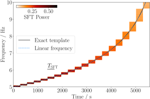
Figure 1: Spectrogram of a GW signal compatible with the inspiral of a $(1.4-1.4)\,\mathrm{M}_{\odot}$ BNS. This corresponds to the squared absolute value of a set of SFTs. Colored regions correspond to frequency ranges where the GW signal is present. As the signal evolves, the frequency increases at a faster rate, broadening the colored frequency ranges. The signal frequency evolution, shown as a solid black curve, is computed using a state-of-the-art time-domain waveform model. The approximated linear frequency, shown as a dashed blue curve, is computed at the beginning of each SFT (white circles). The inner product can be efficiently computed by folding in the complex amplitude of signal-dominated frequency regions in each SFT and accumulating the result over time. We used $T_{\mathrm{SFT}}=$280\text{\,}\mathrm{s}$$, which is unrealistically large (see Sec. IV), to better illustrate the basic idea. On a realistic application the highlighted regions become an order of magnitude narrower.

The use of SFTs is schematically shown in Fig. 1. First, the original dataset is split into “short” time segments which then get Fourier transformed. Each of this segments corresponds to an SFT. The set of all SFTs forms a complex-valued 2D array with a time axis and a frequency axis, whose absolute value squared is to be identified with a spectrogram. At each SFT, the GW signal under study is spread across a narrow frequency range (colored fringes in Fig. 1). In particular, Eq. (1) can be computed by accumulating SFT values at the frequency bins around the signal’ s frequency weighed by an appropriate kernel. Since SFTs are treated independently, the analysis can easily deal with noise non-stationarities, time-dependent modulations induced by the detector, and missing data periods.

We further exploit the slow frequency evolution of long-duration GW to massively downsample the dataset using SFTs once and for all for a given analysis. This reduces the memory footprint of the analysis by up to three to four orders of magnitude, significantly reducing the computing cost and allowing for batch-evaluating likelihoods using hardware accelerators such as GPUs.

Our new approach addresses the three key challenges identified above by construction.

In this paper, we develop the SFT formalism and present a pilot application applied to the early warning of both BNS signals in third-generation ground-based detectors and massive BBH signals in LISA. The computational advantages of SFTs provide a promising approach for low-latency GW analyses targeting multi-messenger science, where every instant gained by GW data-analysis corresponds to new and potentially ground-breaking science on the electromagnetic side [48, 49].

The required tools to operate using the SFTs framework are released as part of an accompanysft open-source software package, sfts [50].

Owing to its simplicity, scalability, and computational efficiency, our SFT approach paves the way for a new paradigm in GW data analysis, offering a powerful framework to tackle challenges to come.

II Gravitational-wave data analysis

II.1 Strain and detector projection

Let us first review the basic tools for the analysis of GW data. GW data analysis operates with a log-likelihood [51]

$$\mathcal{L}(\theta)=\left\langle x,h(\theta)\right\rangle-\frac{1}{2}\left\langle h(\theta),h(\theta)\right\rangle\,,$$ (2)

where $x$ is the observed data and $h(\theta)$ is a signal template characterised by a set of parameters $\theta$. This assumes that (i) the noise is Gaussian and (ii) the power spectral density of the noise can be reasonably estimated. The specific formulation of $\left\langle\cdot,\cdot\right\rangle$ in Eq. (2) depends on the application, namely parameter-estimation routines or detection statistics for search pipelines [15, 51, 45, 52, 53, 54, 55, 56, 57].

In this paper, we treat the problem of long-duration GW signals. We consider signals that start to be observed at an early stage of their inspiral, so that most of their power is narrowly concentrated in the frequency domain at any given time. Signals beyond this regime can still make use of the methods here discussed by excising the inspiral from the rest of the waveform.

We describe a GW signal in terms of phase $\varphi(t)$ and amplitude $A(t)$, which in turn give rise to two polarizations $h_{+}(t)$ and $h_{\times}(t)$. As the signal reaches the detector, the observed strain can be expressed as [51]

$$h(t)=F_{+}(t)h_{+}(t)+F_{\times}(t)h_{\times}(t)$$ (3)

where

$$\begin{bmatrix}F_{+}(t)\\ F_{\times}(t)\end{bmatrix}=\sin\zeta\begin{bmatrix}\cos{2\psi}&\sin{2\psi}\\ -\sin{2\psi}&\cos{2\psi}\end{bmatrix}\begin{bmatrix}a(t)\\ b(t)\end{bmatrix}$$ (4)

are the polarization-dependent antenna patterns, $\psi$ is the polarization angle, $a(t),b(t)$ are the detector-dependent antenna pattern functions, and $\zeta$ is the opening angle of the detector (e.g. $\zeta=90^{\circ}$ for LIGO/Virgo/Kagra). This description of $h(t)$ is appropriate under the so-called long-wavelength approximation, which is valid for current and future ground-based detectors below a few thousand kHz and for LISA up to a few mHz [58, 59, 60]. Let us also define a projector

$$\Lambda_{t} =F_{+}(t)\mathcal{I}_{+}\mathrm{Re}+F_{\times}(t)\mathcal{I}_{\times}\mathrm{Im}$$ (5)

where $\mathcal{I}_{+,\times}$ are orientation and polarization-dependent coefficients such that

$$h(t)=\Lambda_{t}A(t)e^{i\varphi(t)}\,,$$ (6)

abstracting away any dependencies on the number of detectors, the number of modes, and the number of polarizations in the GW signal.

Throughout this work, we will take $\varphi(t)$ and $A(t)$ be consistent with the $(2,\pm 2)$ GW mode of IMRphenomT [61, 62, 63]. Our specific implementation [50], is differentiable and GPU-vectorized using jax [64] as described in Appendix A.

II.2 Detection statistics

In the applications here presented, we are primarily concerned with GW searches. These evaluate a detection statistic, which is usually derived from Eq. (2), on a set of waveform templates in order to determine the presence of a signal.

Current CBC analyses derive a detection statistic by maximizing Eq. (2) with respect to the initial GW phase and distance [15, 18, 52]:

$$\max_{\mathrm{distance},\varphi_{0}}\mathcal{L} =\frac{\left\langle x,h_{\mathrm{c}}\right\rangle^{2}+\left\langle x,h_{\mathrm{s}}\right\rangle^{2}}{\left\langle h_{\mathrm{c}},h_{\mathrm{c}}\right\rangle}\,,$$ (7)

$$h_{\mathrm{c}} =A(t)\cos\varphi(t)\,,$$ (8)

$$h_{\mathrm{s}} =-A(t)\sin\varphi(t)\,.$$ (9)

This approach is based on the fact that, for a short signal, the detector response is constant and the two polarizations cannot be resolved. It also assumes that only the dominant GW mode is present.

For long-duration signals, the amplitude modulations imprinted by the detector cannot be neglected and the two polarizations become distinguishable [56]. This motivates the following parametrization for the observed strain:

$$h(t)=\sum_{\nu=0}^{3}c_{\nu}h_{\nu}(t)\,,$$ (10)

where the four time-dependent functions are given by

$$h_{\nu}(t)=A(t)\begin{bmatrix}a(t)\cos\varphi(t)\\ b(t)\cos\varphi(t)\\ a(t)\sin\varphi(t)\\ b(t)\sin\varphi(t)\end{bmatrix}$$ (11)

and the corresponding time-independent amplitudes are

$$c_{\nu}=\begin{bmatrix}\mathcal{I}_{+}\cos\phi_{0}\cos{2\psi}-\mathcal{I}_{\times}\sin\phi_{0}\sin{2\psi}\\ \mathcal{I}_{+}\cos\phi_{0}\sin{2\psi}+\mathcal{I}_{\times}\sin\phi_{0}\cos{2\psi}\\ -\mathcal{I}_{+}\sin\phi_{0}\cos{2\psi}-\mathcal{I}_{\times}\cos\phi_{0}\sin{2\psi}\\ -\mathcal{I}_{+}\sin\phi_{0}\sin{2\psi}+\mathcal{I}_{\times}\cos\phi_{0}\cos{2\psi}\end{bmatrix}\,.$$ (12)

For a signal with constant amplitude $A(t)=A$, these expressions reduce to the parametrization commonly used in CW searches [51, 65, 66].

Designing a detection statistic à la Eq. (7) in this situation is not so straightforward. The standard choice in the CW literature is the $\mathcal{F}$-statistic [51, 67], which maximises Eq. (2) with respect to $c_{\nu}$:

$$\mathcal{F}\propto\max_{c_{0},c_{1},c_{2},c_{3}}\sum_{\nu=0}^{3}c_{\nu}\left\langle x,h_{\nu}\right\rangle-\frac{1}{2}\sum_{\nu,\mu=0}^{3}c_{\nu}c_{\mu}\left\langle h_{\nu},h_{\mu}\right\rangle\,.$$ (13)

Albeit computationally efficient, said statistic was later found not to be optimal [68, 69]. Other prescriptions have been proposed to deal with different signal and noise hypotheses [69, 70, 71, 72, 45, 73, 74, 56, 57, 75, 76]. For the purposes of this work, we will directly compare inner products in order to assess the accuracy of the SFT framework. The formulation of a suitable detection statistic for long-duration early-warning applications is left to future work.

Throughout this work, we neglect the Doppler modulation of the detector on the signal for the sake of simplicity. As thoroughly shown in Refs. [51, 77, 72, 78, 70, 79, 47] (see Ref. [41] for a review), the required machinery to account for this effect can be seamlessly included into our framework and does not introduce major drawbacks.

III Accelerated inner products

III.1 Broad strategy

With these ingredients, we now derive an efficient implementation of Eq. (1) for long-duration, inspiral-only GW signals. The main assumption is that, within a sufficiently short time segment (to be formalized later), the Fourier transform of $h(t)$ is concentrated within a narrow frequency range. This is similar to the assumptions required when using the stationary phase approximation [80]. We refer to such segmented signals as “quasi-monochromatic.”

Note that any signal with a non-quasi-monochromatic component can be separated into two segments so that the quasi-monochromatic one (which tends to last for longer) is analyzed as in this paper while the rest (which tends to be significantly shorter) is analyzed with traditional methods. For a compact binary, this is the case of an inspiral-merger-ringdown signal, where only the inspiral portion is taken as quasi-monochromatic.

Our goal is to formulate Eq. (1) using SFTs in a similar manner to current implementations of the $\mathcal{F}$-statistic [44, 45, 46]. This approach is desirable for several reasons:

1. Fourier transforms of the data will be computed once and will be valid for any template within a given parameter-space region.

2. Noise non-stationarities can be treated by whitening data on a per-SFT basis.

3. Gaps in the data are automatically accounted for, as they simply correspond to missing SFTs.

4. The number of waveform evaluations will be reduced significantly; rather than once per data sample, they will only be required once per SFT.

Moreover, the use of SFTs significantly reduces the memory footprint of a waveform evaluation, allowing for their batch-evaluation. This makes the SFT formulation suitable for GPU hardware and reduces the computing cost of a GW analysis to an unprecedented level. Computational implications are discussed in Sec. V.

III.2 Quasi-monochromatic signals

We start by expressing Eq. (1) in the time domain:

$$\left\langle d,h\right\rangle=\int_{0}^{T}\mathrm{d}t\,d(t)\,h(t)\,,$$ (14)

where $T$ is the maximum time range so that the signal remains quasi-monochromatic. The time series $d(t)$ entering Eq. (14) is the whitened observed data

$$d(t)\doteq 4\,\mathrm{Re}\int_{0}^{\infty}\mathrm{d}f\frac{\tilde{x}^{*}(f)}{S_{\mathrm{n}}(f)}e^{-2i\pi ft}\,.$$ (15)

The process of whitening a strain dataset has been discussed at length elsewhere [24, 51, 72, 81, 15, 82, 79, 83, 18, 84]. We also assume that backgrounds containing overlapping signals, such as those expected to affect next-generation detectors, have been properly dealt with [85, 86, 87, 88].

Data $d$ is measured on a discrete set of timestamps $\{t_{j}=j\Delta t,j=0,\dots,N-1\}$. We divide the observed data into $N_{\mathrm{SFT}}$ disjoint time segments $\mathcal{T}_{\alpha}=[t_{\alpha},t_{\alpha+1}]$. Each of these segments has a duration of $T_{\mathrm{SFT}}=t_{\alpha+1}-t_{\alpha}$ and contains $n_{\mathrm{SFT}}=T_{\mathrm{SFT}}/\Delta t$ samples. The time $T_{\mathrm{SFT}}$ should be chosen so that the GW phase within a segment can be Taylor-expanded to second order (see Sec. III.4)

$$\varphi(t) \approx\varphi_{\alpha}+\Delta\varphi_{\alpha}(t)\,,$$ (16)

$$\Delta\varphi_{\alpha}(t) =2\pi f_{\alpha}(t-t_{\alpha})+\pi\dot{f}_{\alpha}(t-t_{\alpha})^{2}\,,$$ (17)

where the $\alpha$ subscript denotes evaluation at time $t_{\alpha}$, dots denote time differentiation, and $f_{\alpha}=\dot{\varphi}_{\alpha}$. This implies that for $t\in\mathcal{T}_{\alpha}$, the waveform strain $h(t)$ is described by 4 numbers $\{A_{\alpha},\varphi_{\alpha},f_{\alpha},\dot{f}_{\alpha}\}$ rather than the initial $n_{\mathrm{SFT}}$ samples. In particular one has

$$h_{\alpha}(t)=\begin{cases}A_{\alpha}\Lambda_{\alpha}e^{i[\varphi_{\alpha}+\Delta\varphi_{\alpha}(t)]}&{\rm for}\quad t\in\mathcal{T}_{\alpha}\,,\\ 0&{\rm for}\quad t\notin\mathcal{T}_{\alpha}\,.\end{cases}$$ (18)

such that

$$h(t)\approx\sum_{\alpha=0}^{N_{\mathrm{SFT}}-1}h_{\alpha}(t)\,.$$ (19)

Let us further assume that the evolution of the signal amplitude is slow enough to be approximated as a constant within a segment $\mathcal{T}_{\alpha}$. This involves both the GW amplitude $A_{\alpha}$ and the detector amplitude modulation, here encapsulated in the projector $\Lambda_{\alpha}$. The case for $A_{\alpha}$ is trivial, as we are in the regime of validity of the stationary phase approximation [80]. The detector amplitude modulation varies on a timescale of $\gtrsim 1\,{\rm day}$ ($\gtrsim 1\,{\rm year}$) for ground-(space-)based detectors. These are usually longer than those allowed by the variation of $A_{\alpha}$, so this is not an issue in practice; otherwise, $T_{\mathrm{SFT}}$ needs be chosen according to $\Lambda_{\alpha}$.

Equation (14) can now be expressed as a sum over disjoint time segments:

$$\left\langle d,h\right\rangle =\sum_{\alpha=0}^{N_{\mathrm{SFT}}-1}A_{\alpha}\Lambda_{\alpha}e^{i\varphi_{\alpha}}\left\langle d_{\alpha},e^{i\Delta\varphi_{\alpha}}\right\rangle\,,$$ (20)

$$\left\langle d_{\alpha},e^{i\Delta\varphi_{\alpha}}\right\rangle =\int_{0}^{T_{\mathrm{SFT}}}\mathrm{d}\tau\,d_{\alpha}(\tau)e^{i(2\pi f_{\alpha}\tau+\pi\dot{f}_{\alpha}\tau^{2})}\,,$$ (21)

where we took $d_{\alpha}(\tau)=d(t_{\alpha}+\tau)$. In general, data will be evaluated at discrete times $d_{\alpha}[j]=d(t_{\alpha}+\tau_{j})$ with $\tau_{j}=j\Delta t$. This yields

$$\left\langle d_{\alpha},e^{i\Delta\varphi_{\alpha}}\right\rangle=\Delta t\sum_{j=0}^{n_{\mathrm{SFT}}-1}d_{\alpha}[j]e^{i(2\pi f_{\alpha}\tau_{j}+\pi\dot{f}_{\alpha}\tau_{j}^{2})}\,.$$ (22)

III.3 SFTs and Fresnel kernel

We seek an efficient implementation of Eq. (22). A first naïve attempt would be to interpret it as a discrete Fourier transform of a data segment (i.e. an SFT) with respect to the frequency parameter $f_{\alpha}$. This approach, would make the SFT dependent on the waveform parameters, which would thus need to be recomputed for every waveform across either template banks for GW searches or likelihood evaluations for GW parameter estimation. This would also require keeping the original dataset in memory, without any computing advantages.

Instead, we introduce an arbitrary discrete Fourier frequency $f_{k}=k/T_{\mathrm{SFT}}$ to rewrite Eq. (22) as

$$\left\langle d_{\alpha},e^{i\Delta\varphi_{\alpha}}\right\rangle\!=\!\Delta t\!\sum_{j=0}^{n_{\mathrm{SFT}}-1}\!\!\left\{d_{\alpha}[j]e^{i[2\pi(f_{\alpha}\!-\!f_{k})\tau_{j}+\pi\dot{f}_{\alpha}\tau_{j}^{2}]}\right\}e^{i2\pi\tau_{j}f_{k}}.$$ (23)

This can be interpreted as the SFT of a product of functions evaluated at $f_{k}$. Note also that waveform parameters and data are coupled by a product operation. We can untangle this coupling using the convolution theorem applied to discrete Fourier transforms [89]:

$$\mathcal{C}(f_{\alpha},\dot{f}_{\alpha};\tilde{d}_{\alpha}) \doteq\left\langle d_{\alpha},e^{i\Delta\varphi_{\alpha}}\right\rangle$$

$$=\Delta f\sum_{k=k_{\mathrm{min}}}^{k_{\mathrm{max}}}\tilde{d}_{\alpha}^{*}[k]\,\mathfrak{Fre}(f_{\alpha}-f_{k},\dot{f}_{\alpha})\,,$$ (24)

where

$$\Delta f =T_{\mathrm{SFT}}^{-1}\,,$$ (25)

$$\tilde{d}_{\alpha}[k] =\Delta t\sum_{j=0}^{n_{\mathrm{SFT}}-1}d_{\alpha}[j]e^{-i2\pi\tau_{j}f_{k}}\,,$$ (26)

$$\mathfrak{Fre}(f_{0},f_{1}) =\Delta t\sum_{j=0}^{n_{\mathrm{SFT}}-1}e^{i(2\pi f_{0}\tau_{j}+\pi f_{1}\tau_{j}^{2})}\,.$$ (27)

Equation (26) is the SFT of a data taken within a time segment $\mathcal{T}_{\alpha}$. As long as $T_{\mathrm{SFT}}$ is chosen appropriately, this is independent of the waveform parameters and can be computed only once. Also, we take $\tilde{d}_{\alpha}[k]=0$ for $k<0$.

The summation in Eq. (27) can be expressed in closed form by taking the continuum limit:

$$\mathfrak{Fre}(f_{0},f_{1})=\int_{0}^{T_{\mathrm{SFT}}}\,\mathrm{d}\tau\,e^{i(2\pi f_{0}\tau+\pi f_{1}\tau^{2})}\,.$$ (28)

This is justified as the kernel $\mathfrak{Fre}$ does not involve any inherently discrete terms; in any case, the number of samples in our typical applications will be high enough to justify this step (see e.g. Ref. [90] as well as Appendix B where a similar argument is made for a different kernel). Completing the square we find

$$\mathfrak{Fre}(f_{0},f_{1})=\frac{e^{-i\pi f_{0}^{2}/f_{1}}}{\sqrt{2f_{1}}}\left\{C(u)-C(l)+i[S(u)-S(l)]\right\}\,,$$ (29)

where

$$l =\sqrt{\frac{2}{f_{1}}}f_{0}\,,$$ (30)

$$u =l+\sqrt{2f_{1}}T_{\mathrm{SFT}}\,,$$

and the Fresnel integrals are given by

$$C(x)=\int_{0}^{x}\mathrm{d}\tau\cos{\left(\frac{\pi}{2}\tau^{2}\right)}\,,$$ (31)

$$S(x)=\int_{0}^{x}\mathrm{d}\tau\sin{\left(\frac{\pi}{2}\tau^{2}\right)}\,.$$ (32)

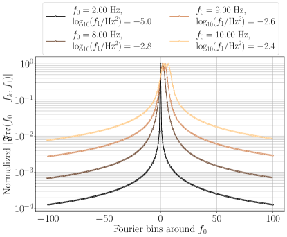
Figure 2: Magnitude of the kernel $\mathfrak{Fre}$ normalized by its maximum value for different values of $f_{0},f_{1}$ taken from the evolution of a $(1.4-1.4)\,\mathrm{M}_{\odot}$ BNS for $T_{\mathrm{SFT}}=$50\text{\,}\mathrm{s}$$. For small values of $f_{1}$, the signal is practically monochromatic and $\mathfrak{Fre}$ narrows down to the Dirichlet kernel (see Appendix B). For positive values of $f_{1}$, the signal visibly drifts towards higher frequencies.

The summation on the frequency index $k$ in Eq. (24) should run over the full frequency spectrum. As shown in Fig. 2, however, the kernel $\mathfrak{Fre}$ falls off rapidly for values of $f_{0}$ away from zero, allowing for the summation to be safely truncated to a finite range $k\in[k_{\mathrm{min}},k_{\mathrm{max}}]$ around $f_{k}\sim f_{\alpha}$. This is comparable to the truncation of the Dirichlet kernel described in Refs. [44, 90, 46].

III.4 SFT length

The computations presented above require a suitable choice of $T_{\mathrm{SFT}}$. To this end, we follow a well-established criterion in CW searches [72], namely that the frequency evolution described by Eq. (19) deviates by less than a certain fraction $\delta$ of the SFT frequency resolution $\Delta f$. For a linear frequency evolution, the corresponding Taylor residual $R$ is bounded by

$$\left|R\right|\leq\frac{1}{2}T_{\mathrm{SFT}}^{2}\max_{\alpha}\ddot{f}_{\alpha}\,.$$ (33)

The maximum allowed $T_{\mathrm{SFT}}$ thus corresponds to $\left|R\right|=\delta\Delta f$, which implies

$$T_{\mathrm{SFT}}(\delta)=\left(\frac{2\delta}{\max_{\alpha}\ddot{f}_{\alpha}}\right)^{1/3}\,.$$ (34)

For CBC signals, $T_{\mathrm{SFT}}$ will be dominated by values of $\ddot{f}_{\alpha}$ at the end of the inspiral. This choice is not unique; rather, $\delta$ should be chosen such that the corresponding $T_{\mathrm{SFT}}$ is valid for as many waveforms as possible.

III.5 Main takeaways

The framework put forward in this paper corresponds to approximating the inner product $\left\langle d,h\right\rangle$ with

$$\left(\left[d,h\right]\right)\doteq\Delta f\sum_{\alpha=0}^{N_{\mathrm{SFT}}-1}A_{\alpha}\Lambda_{\alpha}e^{i\varphi_{\alpha}}\mathcal{C}(f_{\alpha},\dot{f}_{\alpha};\tilde{d}_{\alpha})\,.$$ (35)

This formulation of the inner product can be intuitively interpreted as follows (see Fig. 1). First, the original dataset is processed into a set of SFTs, which we can think of as a 2D array with a time axis and a frequency axis (more precisely, SFTs can be interpreted as a complex spectrogram, which becomes a standard spectrogram after taking their squared absolute value). To compute the inner product of a quasi-monochromatic signal, we follow its instantaneous frequency as a function of time across the spectrogram, and add the Fourier amplitudes coherently. From a computational point of view, this is a coherent version of the CW search strategy put forward in Ref. [47] by one of the authors.

Note that the data are the only quantity whose Fourier transform is ever computed. All waveform quantities are evaluated in the time domain.

IV Applications

IV.1 Accuracy metric

We now present two pilot applications of the SFT framework, considering early warnings for BNS in third-generation ground-based detectors and massive BBH in LISA. While these applications are mainly restricted to CBC signals in their inspiral, we stress the methodology presented here can be combined with other strategies to include further stages that break quasi-monochromaticity.

Concretely, we will assess the error due to using $\left(\left[d,h\right]\right)$ instead of $\left\langle d,h\right\rangle$ using the relative error:

$$r=1-\sqrt{\frac{\left(\left[d,h\right]\right)}{\left\langle d,h\right\rangle}}\,.$$ (36)

This quantity is comparable to the mismatch of a template bank [91, 92, 93, 94], which represents the fractional loss in detection statistic due to placing a finite number of templates in a continuous space. The maximum allowed mismatch depends on the source under analysis, with current CBC searches aiming for a maximum mismatch of $1\%$ to $3\%$ [95, 96, 97, 98].

The result of this analysis will be a quantification of the loss produced by the approximations used in $\left(\left[\cdot,\cdot\right]\right)$ with respect to $\left\langle\cdot,\cdot\right\rangle$. To do so, we generate a time series containing a fiducial signal and compute $\left\langle d,h\right\rangle$ by direct integration. We then compute $r$ for different values of $\delta$ and $\Delta k=k_{\mathrm{max}}-k_{\mathrm{min}}$. Acceptable setups will correspond to those so that $r\lesssim 1\%$. In general, more permissive setups (higher $r$) yield computationally cheaper implementations.

$\delta$	3.0	2.5	2.0	1.5	1.0	0.5
$T_{\mathrm{SFT}}/\mathrm{s}$	106	99	92	84	73	58
$N_{\mathrm{SFT}}$	4396	4707	5066	5548	6384	8035

Table 1: SFT configurations for a BNS signal from $1\text{\,}\mathrm{Hz}$ to $40\text{\,}\mathrm{Hz}$ as described in Sec. IV.2. The corresponding loss $r$ is shown in Fig. 3.

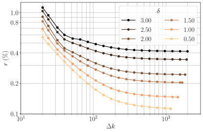
Figure 3: Relative error for a $(1.4-1.4)\,\mathrm{M}_{\odot}$ BNS as described in Sec. IV.2 for different choices of $\delta$ and $\Delta k$.

IV.2 Early warning for BNS mergers in third-generation ground-based detectors

As a first application, we simulate an early-alert search for a BNS system. The two objects have masses of $1.4\text{\,}\mathrm{M_{\odot}}$, corresponding to a chirp mass of $\mathcal{M}=$1.21\text{\,}\mathrm{M_{\odot}}$$. The signal is observed from $1\text{\,}\mathrm{Hz}$ up to $10\text{\,}\mathrm{Hz}$, with a sampling frequency of $40\text{\,}\mathrm{Hz}$. This frequency band is consistent with future-generation detectors such as Einstein Telescope [9] and Cosmic Explorer [10]. This results in about $N_{0}\approx 2\times 10^{7}$ data points spanning a total of $130$ hours.

We assume the orientation and sky position of this source is compatible with the projector

$$\Lambda_{t}=[a(t)+b(t)](\mathrm{Re}+\mathrm{Im})\,,$$ (37)

where we took $c_{\nu}=1$ and

$$a(t)=\cos{\left(2\pi t/1\,\mathrm{day}\right)}\,,$$ (38)

$$b(t)=\sin{\left(2\pi t/1\,\mathrm{day}\right)}\,,$$ (39)

which qualitatively reproduce the expected daily amplitude modulation due to the detector motion. We numerically explore a range of $\delta$ and $\Delta k$ as listed in Table 1. In this particular case, $\max_{\alpha}\ddot{f}_{\alpha}\approx$5\text{\times}{10}^{-6}\text{\,}\mathrm{Hz}\mathrm{/}\mathrm{s}^{2}$$.

As shown in Fig. 3, most configurations with $\delta\lesssim 3$ and $\Delta k\gtrsim 20$ yield acceptable relative errors ($r<1\%$). This is equivalent to a number of SFTs of about $N_{\mathrm{SFT}}\sim 10^{3-4}$. Compared to $N_{0}\sim 10^{7}$, the number of points at which the waveform must be evaluated has dropped by 3 to 4 orders of magnitude. In other terms, this corresponds to diminishing the sampling frequency from $40\text{\,}\mathrm{Hz}$ to $T_{\mathrm{SFT}}^{-1}\sim(0.01-0.1)\mathrm{Hz}$.

$\delta$	1.0	0.5	0.25	0.1	0.05	0.01
$T_{\mathrm{SFT}}/\mathrm{s}$	1735	1377	1092	805	639	373
$N_{\mathrm{SFT}}$	2222	2799	3530	4789	6033	10336

Table 2: SFT configurations for a massive BBH signal from ${10}^{-4}\text{\,}\mathrm{Hz}$ to ${10}^{-3}\text{\,}\mathrm{Hz}$ as described in Sec. IV.3. The corresponding loss $r$ is shown in Fig. 4.

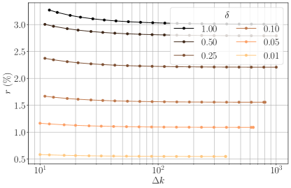
Figure 4: Relative error for a $(10^{6}-10^{6})\,\mathrm{M}_{\odot}$ massive BBH as described in Sec. IV.3 for different choices of $\delta$ and $\Delta k$.

IV.3 Early warning for massive BBH mergers in LISA

As a second application, we consider a massive BBH as observed by the space detector LISA [11]. In this case, we take the two black holes to have a mass of $10^{6}\mathrm{M}_{\odot}$ each and no spin. The system is observed from ${10}^{-4}\text{\,}\mathrm{Hz}$, corresponding to the start of the LISA sensitive band, up to $1.9\text{\times}{10}^{-3}\text{\,}\mathrm{Hz}$, which is the frequency of the Minimum Energy Circular Orbit (MECO) of the system [99]. This is the frequency at which IMRphenomT [61, 62, 63] terminates the inspiral phase and, as a result, is a good proxy for the end of the quasi-monochromatic behavior. This signal last for about 45 days. At a sampling frequency of $2\text{\,}\mathrm{Hz}$, which corresponds to the minimum acceptable sampling frequency covering the full LISA sensitive band [11], this corresponds to $N_{0}\approx 7.5\times 10^{6}$ samples.

The sub-millihertz frequency band is well in the regime of validity of the long-wavelength approximation [59], which allows us to treat LISA as a LIGO-like detector with a yearly amplitude modulation

$$a(t)=\cos{\left(2\pi t/{1\,\mathrm{year}}\right)}\,,$$ (40)

$$b(t)=\sin{\left(2\pi t/{1\,\mathrm{year}}\right)}\,.$$ (41)

This is qualitatively correct, but note we are ignoring the Doppler modulation on the waveform as previously mentioned. Similarly to the previous example, we take $c_{\nu}=1$.

As shown in Fig. 4, in this case $r\approx 1\%$ is achieved at $\delta=0.05$ and $\Delta k\sim 10^{2}$, which corresponds to $T_{\mathrm{SFT}}\approx$10\text{\,}\mathrm{min}$$ and $N_{\mathrm{SFT}}\approx 6\times 10^{3}$ (see Table 2). Once more, this is a reduction of about three orders of magnitude in the number of time samples.

Crucially, the overall data analysis strategy for LISA data will be qualitatively different from that of LIGO/Virgo/KAGRA, since the sheer amount of sources in band calls for the use of a global-fit strategy [100, 101, 102, 103]. Nevertheless, the framework we present here can still play a role in such analyses due to the significant reduction in the required memory size and the advantages in dealing with non-stationarities and gaps in the data compared to the use of bare time-domain or frequency-domain data.

IV.4 Edge effects

For $\delta=1$ and $\Delta k=200$, the relative error $r$ increases by about an order of magnitude between our BNS ($r\approx 0.2\%$) and massive BBH ($r\approx 3\%$) examples. This is due to one of the underlying assumptions of the convolution theorem, namely that the involved sequences are periodic [89]. As mentioned in Sec. III, $d_{\alpha}[k]$ is in general non-periodic as we take $d_{\alpha}[k]=0$ whenever $k<0$.

For a BNS ($T_{\mathrm{SFT}}=$50\text{\,}\mathrm{s}$$), the frequency bin $k_{0}$ corresponding to its minimum frequency ($1\text{\,}\mathrm{Hz}$) is $k_{0}=$50\text{\,}\mathrm{s}$\times$1\text{\,}\mathrm{Hz}$\approx 50$. The edge of the SFT ($k=0$) thus corresponds to $\Delta k=-k_{0}$, which, as shown in Fig. 5, returns a value of $\mathfrak{Fre}$ which is three to four orders of magnitude smaller than that for $\Delta k\sim 0$, thus suppressing edge effects.

For a massive BBH starting at $0.1\text{\,}\mathrm{mHz}$, one has $T_{\mathrm{SFT}}\sim 10^{2-3}\,\mathrm{s}$, which implies $k_{0}=10^{2-3}\times${10}^{-4}\text{\,}\mathrm{Hz}$\approx 0$, i.e. the signal is located at the edge of the SFT. As a result, the information around $k_{0}$ which would be recovered through the Fresnel kernel is lost, increasing the relative error. Lowering $\delta$ (i.e. shortening $T_{\mathrm{SFT}}$) ameliorates this problem: the SFT frequency resolution becomes coarser and the signal behaves closer to a monochromatic signal. This can be seen in Fig. 5, where for a shorter $T_{\mathrm{SFT}}$ the kernel $\mathfrak{Fre}$ drops by about an order of magnitude away from $|f_{0}-f_{k}|\approx 0$, thus down-weighting the contribution from any side bands. This behavior denotes that the signal is closer to a monochromatic one for a shorter $T_{\mathrm{SFT}}$ (see App. B). The result is a difference by a factor of 3 in the number of time samples ($\approx 6000$ vs. $\approx 2000$) which, while important, is still sub-dominant when compared to the overall reduction of three orders of magnitude achieved with our framework.

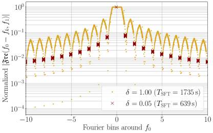
Figure 5: Comparison of the kernel $\mathfrak{Fre}$ throughout the evolution of a massive BBH for different values of $\delta$. We compute $\mathfrak{Fre}$ for all $(f_{\alpha},\dot{f}_{\alpha})$ from ${10}^{-4}\text{\,}\mathrm{Hz}$ to $1.9\text{\times}{10}^{-3}\text{\,}\mathrm{Hz}$ for a $(10^{6}-10^{6})\mathrm{M}_{\odot}$ system. The frequency resolution is $T_{\mathrm{SFT}}^{-1}\approx$0.8\text{\,}\mathrm{mHz}$$ ($T_{\mathrm{SFT}}^{-1}=$0.02\text{\,}\mathrm{Hz}$$) for $\delta=1.00$ ($\delta=0.05$). The vertical axis is normalized to the maximum value as in Fig. 2.

V Computational implications

There are three key computational advantages in our implementation of the GW inner product.

V.1 SFTs

The advantages of SFTs with respect to time-domain or frequency-domain representations have been outlined in Sec. III. This data format is also advantageous from a computing perspective.

In a GW experiment, data is naturally taken as a time series containing $N_{0}$ samples. Obtaining a frequency domain representation of this dataset involves $\mathcal{O}(N_{0}\log N_{0})$ operations using a Fast Fourier Transform, and requires storing complete dataset before this operation can be performed.

Similarly, the cost of computing an SFT using the Fast Fourier Transform (FFT) scales as $\mathcal{O}(n_{\mathrm{SFT}}\log n_{\mathrm{SFT}})$. These can be computed online and in parallel as data arrives at the detector, allowing for analyses with very low latency. Moreover, the cost of computing all the SFTs in a dataset scales as $\mathcal{O}(N_{0}\log n_{\mathrm{SFT}})$, which is lower than computing the full transform by a factor $\log{N_{0}}/\log{n_{\mathrm{SFT}}}\sim 2$ according to the results in Sec. IV.

This shows that SFTs are an appropriate and efficient representation, in a similar manner to wavelets [40], to analyze data streams with time-dependent statistical properties.

V.2 Scalar-product evaluation

Within the SFT framework, evaluating the approximate inner product $\left(\left[\cdot,\cdot\right]\right)$ involves two steps:

1. Evaluate waveform quantities $\{A_{\alpha},\varphi_{\alpha},f_{\alpha},\dot{f}_{\alpha}\}$ across SFTs.

2. Weight and sum the relevant SFT bins according to Eq. (35).

Note that SFTs can be computed once in advance and then reused for a given parameter-space region.

Without the SFT framework, waveforms in step (i) must be evaluated at each of the $\mathcal{O}(N_{0})$ time samples, unless their implementation is capable of benefiting from an acceleration scheme [33, 34, 35, 36, 37, 38, 39]. The SFT framework, on the other hand, only requires to evaluate a time-domain waveform on $\mathcal{O}(N_{\mathrm{SFT}})$ time samples. As shown in Sec. IV, $N_{0}/N_{\mathrm{SFT}}\sim 10^{3-4}$. For waveforms such as IMRphenomT [63, 62, 61], which are implemented using closed-form expressions, this implies the SFT framework outright reduces their computing cost and memory requirements by three to four orders of magnitude.

Step (ii) involves adding $\mathcal{O}(\Delta k\times N_{\mathrm{SFT}})$ bins after computing their corresponding weights using $\mathfrak{Fre}$ and $\Lambda_{\alpha}$. Results in Sec. IV show $\Delta k\sim 10^{2}$ to be an acceptable value. As a result, in terms of number of operations, $\Delta k\times N_{\mathrm{SFT}}\sim 10^{5-6}$ is one to two orders of magnitude lower than the direct integration given by Eq. (1), which involves $N_{0}\sim 10^{7}$ frequency bins.

Overall, given a closed-form time-domain waveform model, evaluating the SFT-based inner product $\left(\left[\cdot,\cdot\right]\right)$ instead of $\left\langle\cdot,\cdot\right\rangle$ results in a reduction of three to four orders of magnitude in both waveform evaluation time and memory footprint, and a reduction of one to two orders of magnitude in computing the inner product.

V.3 Vectorized inner product

The gains in computing cost and memory consumption reported in the previous subsection suggest GPU parallelization as a promising approach to further accelerate the evaluation of Eq. (35).

In this work, both IMRphenomT and $\left(\left[\cdot,\cdot\right]\right)$ have been implemented as part of the sfts package [50] using jax [64], a high-level python front end which allows for just-in-time compilation, GPU acceleration, and, crucially, automatic vectorization.

To parallelize Eq. (35) on a GPU, we use the vmap instruction in jax, which transforms a waveform operating on a single set of parameters into a waveform operating on batches of parameters. The implementation is otherwise unchanged. The maximum batch size (i.e. how many waveforms are processed in parallel) of course depends on the computing capabilities of the machine at hand.

To test the computing cost, we generate a batch of waveforms using our re-implementation of the inspiral portion of IMRphenomT by randomly sampling masses within 1% of the examples previously described and evaluating Eq. (35). We perform all our tests using a 13th Gen Intel(R) Core(TM) i7-1355U CPU and a NVIDIA H100 64GB GPU.

1. For the BNS case ($\delta=1.0,\,\Delta k=100$), the computing cost of evaluating Eq. (35) for a single waveform using a CPU is $0.1\text{\,}\mathrm{s}$. Using vmap we can evaluate Eq. (35) for a batch of 100 waveforms, with an average cost of $0.07\text{\,}\mathrm{s}$ per waveform. On a GPU, we can extend the batch size to 1000 with an average cost of $0.2\text{\,}\mathrm{ms}$ per waveform.

2. For the massive BBH case ($\delta=0.05,\,\Delta k=10$), Eq. (35) for a single waveform on a CPU takes $0.01\text{\,}\mathrm{s}$. The batch size on a CPU in this case can be increased up to 1000 waveforms, yielding an average cost of $3\text{\,}\mathrm{ms}$ per waveform. On a GPU with a batch size of 1000 waveforms the average computing cost drops to $0.01\text{\,}\mathrm{ms}$ per waveform.

These GPU applications, which have been made possible by the SFT framework, demonstrate a further computing cost reduction of two to three orders of magnitude due to jax’s vmap primitive with virtually no development cost. Altogether, whenever applicable, the SFT framework results in a reduction of three to five orders of magnitude in computing Eq. (1) with respect to other formulations. These results are complementary to those of Ref. [104], which evaluate a single waveform including the merger and ringdown phases on a GPU.

VI Conclusion

We presented a new framework based on SFTs to analyze long-duration GW signals emitted by compact objects in binary systems. This is one of the key data-analysis challenges posed by next-generation GW detectors [9, 10, 11].

The basic idea, shown in Fig. 1, is to Fourier transform short disjoint segments (producing SFTs) so that waveform templates can be filtered against the relevant portion of the data spectrum at different times in their evolution. This approach is inspired by CW search methods [44, 45, 46] and provides several computational advantages at a negligible development cost.

Since SFTs are disjoint in time, noise non-stationarities can be dealt with on a per-SFT basis [24, 51, 72, 81, 15, 82, 79, 18, 84]. In a similar fashion, gaps in the data simply correspond to missing SFTs. Finally, as thoroughly shown in the CW literature [41, 42, 43], amplitude and frequency modulations caused by the GW detector can be accounted for in time domain on a per-SFT basis as well, vastly reducing the complexity of the analyses with respect to frequency-domain approaches [29]. SFTs can be computed on-line as data arrives and is more efficient than generating the full-time Fourier transform. Furhtermore, they can be recycled for a broad region of the parameter space, further amortizing their minimal implementation cost. In this aspect, they offer comparable advantages to other time-frequency methods [40].

In addition, SFTs allow for a reduction of three to five orders of magnitude in the computing cost of the inner product [Eq. (1)] for inspiral waveforms, which is the most fundamental quantity in any GW data-analysis routine [24, 23]. This gain can be explained by two components:

1. First, the phase evolution of an inspiral waveform within an SFT can be approximated in closed form by a quadratic Taylor expansion. This reduces the effective sampling frequency of a waveform by three to four orders of magnitude and the computing cost of the inner product by one to two orders of magnitude.

2. Second, the reduced sampling frequency, combined with the inherently parallel evaluation of Eq. (1) using the SFT framework [Eq. (14)], allow for the parallelization of multiple waveforms using a GPU. This lowers the computing cost of Eq. (14) further by two to three orders of magnitude.

Overall, we find a cost on the order of $(0.01-0.1)\,\mathrm{ms}$ per inner product evaluation for next-generation GW analysis, depending on the specific application, using current GPUs. As discussed in e.g. Ref. [105, 106, 107], template banks, and in general the computing cost of GW data-analysis routines, may grow by several orders of magnitude for next-generation detectors compared to LIGO/Virgo/KAGRA. This makes the methods presented in this work critical to exploit the scientific capabilities of those GW observatories.

Although the computing advantages we achieved focus on inspiral-dominated signals, the SFT framework can be seamlessly combined with standard methods to tackle the merger and ringdown portions of the waveform. Due to their relatively shorter duration, these are less affected by the difficulties encountered in the inspiral (see e.g. Ref [59]).

While we have limited this presentation to use a single detector and a single GW mode, the SFT framework can operate with multiple detectors and GW modes by extending the definition of the projector operator, much like in other CW analysis pipelines.

The SFT framework crucially relies on evaluating waveform amplitudes, phases, frequencies, and frequency derivatives at arbitrary times. This requirement is incompatible with the current interface exposed by the LIGO Algorithm Library [108, 109]; as a result, we re-implemented the closed-form time-domain inspiral portion of IMRphenomT  [61, 62, 63] using jax to allow for automatic parallelization and differentiation operations, which we release under the sfts [50] package together with the required tools to operate within the SFT framework. This release complements other efforts in the community focused on frequency-domain models [110, 111] and cements vectorized waveforms as a crucial tool for the acceleration of GW data-analysis workflows [47].

The SFT framework, however, is not limited to closed-form waveform approximants. Any waveform family [25, 27, 28] capable of providing the required ingredients can benefit from the computing advantages here discussed. Future work will investigate extensions and limitations of the SFT framework to operate on precessing and/or eccentric waveform models, as well as other more intricate sources such as extreme mass-ratio inspirals [13]. These kinds of phenomena are often described in the time-domain [104], which is precisely the input domain expected by the SFT framework.

In addition, the SFT framework can serve as a basis to further accelerate alternative strategies, such as the semicoherent methods proposed for BNS early-warning searches [106], stellar-mass BBHs in LISA [112], extreme mass-ratio inspirals [113, 114, 115, 116], or long transient GW from young neutron stars [117]. Moreover, using Fresnel integrals may reduce the number of required SFTs in a CW search, further lowering the cost of their semicoherent approaches [46, 45].

Taken together, these results provide a promising solution to the problem of analyzing the long-duration inspirals observed by next-generation detectors including the effect of noise non-stationaries, data gaps, and modulations induced by the detector motion.

Appendix A Vectorized inspiral time-domain waveform

The LIGO Algorithm Library (lalsuite) [108, 109] provides a Python interface to several waveform models available in the literature. Due to its generality, however, it is difficult to freely access the inner workings of a waveform model. For example, in the case of IMRphenomT [61, 62, 63] it is not possible to evaluate $h_{+,\times}$ at an arbitrary time array even though $h_{+,\times}$ are defined as closed-form functions of time. This not only prevents sample-efficient algorithms (such as the one presented here), but also needlessly complicates the use of GPU-parallelization through a python front-end such as jax [64] or pytorch [118].

For this reason, we have re-implemented the inspiral part of the dominant $(2,\pm 2)$ mode of the IMRphenomT approximant using jax. Our implementation is distributed via the sfts [50] package.

Two main advantages result from our re-implementation. First, jax’s automatic differentiation simplifies the computation of $\dot{f}_{\alpha}$ and $\ddot{f}_{\alpha}$ using the closed-form implementation of $\varphi(t)$ or $f(t)$. Second, jax’s vmap primitive allows for the vectorization of $h_{+,\times}$ with respect to both time and waveform parameters. When combined with just-in-time compilation and GPU-support, this allows for an unprecedented speed up in waveform evaluation as discussed in Sec. V.

Appendix B Linear phase drift

The case of a monochromatic signal (i.e. $\dot{f}_{\alpha}=0$) was thoroughly discussed in Ref. [90]. The procedure is similar to the $\dot{f}_{\alpha}\neq 0$ case:

$$\mathcal{C}(f_{\alpha};\tilde{d}_{\alpha})=\Delta f\sum_{k=k_{\mathrm{min}}}^{k_{\mathrm{max}}}\tilde{d}^{*}[k]\,\mathfrak{Dir}(f_{\alpha}-f_{k})\,,$$ (42)

where $\mathfrak{Dir}$ is the Dirichlet Kernel

$$\mathfrak{Dir}(f)=\sum_{j=0}^{n_{\mathrm{SFT}}-1}e^{i2\pi\tau_{j}f_{k}}=n_{\mathrm{SFT}}e^{i\pi T_{\mathrm{SFT}}f}\mathrm{sinc}(T_{\mathrm{SFT}}f)\,,$$ (43)

where $\mathrm{sinc}(x)=\sin{(\pi x)}/(\pi x)$ and the latest equality holds in the limit $n_{\mathrm{SFT}}\gg 1$. Comparing with Eq. (24), $\mathfrak{Fre}$ reduces to $\mathfrak{Dir}$ in the limit $f_{1}=0$.

The $\mathfrak{Dir}$ kernel drops off significantly already at $\Delta k\lesssim 5$ [90]. This is consistent with the early stages of a BNS in Fig. 3; see also Fig. 5, where shorter $T_{\mathrm{SFT}}$ values produced narrower $\mathfrak{Fre}$ kernels as the signals within the SFTs became closer to monochromatic ones.

References

- Abbott et al. [2023] R. Abbott et al., Phys. Rev. X 13, 041039 (2023), arXiv:2111.03606 [gr-qc] .
- Nitz et al. [2023] A. H. Nitz, S. Kumar, Y.-F. Wang, S. Kastha, S. Wu, M. Schäfer, R. Dhurkunde, and C. D. Capano, Astrophys. J. 946, 59 (2023), arXiv:2112.06878 [astro-ph.HE] .
- Wadekar et al. [2023] D. Wadekar, J. Roulet, T. Venumadhav, A. K. Mehta, B. Zackay, J. Mushkin, S. Olsen, and M. Zaldarriaga, (2023), arXiv:2312.06631 [gr-qc] .
- Koloniari et al. [2024] A. E. Koloniari, E. C. Koursoumpa, P. Nousi, P. Lampropoulos, N. Passalis, A. Tefas, and N. Stergioulas, (2024), arXiv:2407.07820 [gr-qc] .
- Aasi et al. [2015] J. Aasi et al., Class. Quant. Grav. 32, 074001 (2015), arXiv:1411.4547 [gr-qc] .
- Acernese et al. [2015] F. Acernese et al., Class. Quant. Grav. 32, 024001 (2015), arXiv:1408.3978 [gr-qc] .
- Akutsu et al. [2019] T. Akutsu et al., Nature Astron. 3, 35 (2019), arXiv:1811.08079 [gr-qc] .
- Maggiore [2007] M. Maggiore, Gravitational Waves. Vol. 1: Theory and Experiments (Oxford University Press, 2007).
- Maggiore et al. [2020] M. Maggiore et al. (ET), JCAP 03, 050, arXiv:1912.02622 [astro-ph.CO] .
- Reitze et al. [2019] D. Reitze et al., Bull. Am. Astron. Soc. 51, 035 (2019), arXiv:1907.04833 [astro-ph.IM] .
- Colpi et al. [2024] M. Colpi et al., (2024), arXiv:2402.07571 [astro-ph.CO] .
- Katz et al. [2020] M. L. Katz, L. Z. Kelley, F. Dosopoulou, S. Berry, L. Blecha, and S. L. Larson, Mon. Not. Roy. Astron. Soc. 491, 2301 (2020), arXiv:1908.05779 [astro-ph.HE] .
- Babak et al. [2017] S. Babak, J. Gair, A. Sesana, E. Barausse, C. F. Sopuerta, C. P. L. Berry, E. Berti, P. Amaro-Seoane, A. Petiteau, and A. Klein, Phys. Rev. D 95, 103012 (2017), arXiv:1703.09722 [gr-qc] .
- Littenberg and Yunes [2019] T. B. Littenberg and N. Yunes, Class. Quant. Grav. 36, 095017 (2019), arXiv:1811.01093 [gr-qc] .
- Allen et al. [2012] B. Allen, W. G. Anderson, P. R. Brady, D. A. Brown, and J. D. E. Creighton, Phys. Rev. D 85, 122006 (2012), arXiv:gr-qc/0509116 .
- Harry and Fairhurst [2011] I. W. Harry and S. Fairhurst, Phys. Rev. D 83, 084002 (2011), arXiv:1012.4939 [gr-qc] .
- Veitch et al. [2015] J. Veitch et al., Phys. Rev. D 91, 042003 (2015), arXiv:1409.7215 [gr-qc] .
- Usman et al. [2016] S. A. Usman et al., Class. Quant. Grav. 33, 215004 (2016), arXiv:1508.02357 [gr-qc] .
- Ashton et al. [2019] G. Ashton et al., Astrophys. J. Suppl. 241, 27 (2019), arXiv:1811.02042 [astro-ph.IM] .
- Chu et al. [2022] Q. Chu et al., Phys. Rev. D 105, 024023 (2022), arXiv:2011.06787 [gr-qc] .
- Cannon et al. [2021] K. Cannon et al., SoftwareX 14, 100680 (2021).
- Huang et al. [2024] Y.-J. Huang et al., (2024), arXiv:2410.16416 [gr-qc] .
- Thorne [1987] K. S. Thorne, in Three Hundred Years of Gravitation (Cambridge University Press, 1987) pp. 330–458.
- Finn [1992] L. S. Finn, Phys. Rev. D 46, 5236 (1992), arXiv:gr-qc/9209010 .
- Varma et al. [2019] V. Varma, S. E. Field, M. A. Scheel, J. Blackman, D. Gerosa, L. C. Stein, L. E. Kidder, and H. P. Pfeiffer, Phys. Rev. Research. 1, 033015 (2019), arXiv:1905.09300 [gr-qc] .
- Pratten et al. [2020] G. Pratten, S. Husa, C. Garcia-Quiros, M. Colleoni, A. Ramos-Buades, H. Estelles, and R. Jaume, Phys. Rev. D 102, 064001 (2020), arXiv:2001.11412 [gr-qc] .
- Ramos-Buades et al. [2023] A. Ramos-Buades, A. Buonanno, H. Estellés, M. Khalil, D. P. Mihaylov, S. Ossokine, L. Pompili, and M. Shiferaw, Phys. Rev. D 108, 124037 (2023), arXiv:2303.18046 [gr-qc] .
- Nagar et al. [2024] A. Nagar, R. Gamba, P. Rettegno, V. Fantini, and S. Bernuzzi, Phys. Rev. D 110, 084001 (2024), arXiv:2404.05288 [gr-qc] .
- Chen and Johnson-McDaniel [2024] A. Chen and N. K. Johnson-McDaniel, (2024), arXiv:2407.15732 [astro-ph.IM] .
- Davis et al. [2021] D. Davis et al., Class. Quant. Grav. 38, 135014 (2021), arXiv:2101.11673 [astro-ph.IM] .
- Soni et al. [2024] S. Soni et al., (2024), arXiv:2409.02831 [astro-ph.IM] .
- Kumar et al. [2022] S. Kumar, A. H. Nitz, and X. J. Forteza, (2022), arXiv:2202.12762 [astro-ph.IM] .
- Vinciguerra et al. [2017] S. Vinciguerra, J. Veitch, and I. Mandel, Class. Quant. Grav. 34, 115006 (2017), arXiv:1703.02062 [gr-qc] .
- García-Quirós et al. [2021] C. García-Quirós, S. Husa, M. Mateu-Lucena, and A. Borchers, Class. Quant. Grav. 38, 015006 (2021), arXiv:2001.10897 [gr-qc] .
- Morisaki [2021] S. Morisaki, Phys. Rev. D 104, 044062 (2021), arXiv:2104.07813 [gr-qc] .
- Zackay et al. [2018] B. Zackay, L. Dai, and T. Venumadhav, (2018), arXiv:1806.08792 [astro-ph.IM] .
- Leslie et al. [2021] N. Leslie, L. Dai, and G. Pratten, Phys. Rev. D 104, 123030 (2021), arXiv:2109.09872 [astro-ph.IM] .
- Krishna et al. [2023] K. Krishna, A. Vijaykumar, A. Ganguly, C. Talbot, S. Biscoveanu, R. N. George, N. Williams, and A. Zimmerman, (2023), arXiv:2312.06009 [gr-qc] .
- Cornish [2021] N. J. Cornish, Phys. Rev. D 104, 104054 (2021), arXiv:2109.02728 [gr-qc] .
- Cornish [2020] N. J. Cornish, Phys. Rev. D 102, 124038 (2020), arXiv:2009.00043 [gr-qc] .
- Tenorio et al. [2021] R. Tenorio, D. Keitel, and A. M. Sintes, Universe 7, 474 (2021), arXiv:2111.12575 [gr-qc] .
- Riles [2023] K. Riles, Living Rev. Rel. 26, 3 (2023), arXiv:2206.06447 [astro-ph.HE] .
- Wette [2023] K. Wette, Astropart. Phys. 153, 102880 (2023), arXiv:2305.07106 [gr-qc] .
- Williams and Schutz [2000] P. R. Williams and B. F. Schutz, AIP Conf. Proc. 523, 473 (2000), arXiv:gr-qc/9912029 .
- Prix et al. [2011] R. Prix, S. Giampanis, and C. Messenger, Phys. Rev. D 84, 023007 (2011), arXiv:1104.1704 [gr-qc] .
- Prix [2019] R. Prix, LIGO Document T0900149 (2019), dcc.ligo.org/LIGO-T0900149.
- Tenorio et al. [2024] R. Tenorio, J.-R. Mérou, and A. M. Sintes, (2024), arXiv:2411.18370 [gr-qc] .
- Abbott et al. [2017] B. P. Abbott et al., Phys. Rev. Lett. 119, 161101 (2017), arXiv:1710.05832 [gr-qc] .
- Mangiagli et al. [2022] A. Mangiagli, C. Caprini, M. Volonteri, S. Marsat, S. Vergani, N. Tamanini, and H. Inchauspé, Phys. Rev. D 106, 103017 (2022), arXiv:2207.10678 [astro-ph.HE] .
-
Tenorio [2025]
R. Tenorio, github.com/rodrigo-tenorio/sfts,
doi.org/10.5281/zenodo.14879509 (2025). - Jaranowski et al. [1998] P. Jaranowski, A. Krolak, and B. F. Schutz, Phys. Rev. D 58, 063001 (1998), arXiv:gr-qc/9804014 .
- Capano et al. [2016] C. Capano, I. Harry, S. Privitera, and A. Buonanno, Phys. Rev. D 93, 124007 (2016), arXiv:1602.03509 [gr-qc] .
- Thrane and Talbot [2019] E. Thrane and C. Talbot, Publ. Astron. Soc. Aust. 36, e010 (2019).
- Christensen and Meyer [2022] N. Christensen and R. Meyer, Rev. Mod. Phys. 94, 025001 (2022), arXiv:2204.04449 [gr-qc] .
- Chua [2022] A. J. K. Chua, Phys. Rev. D 106, 104051 (2022), arXiv:2205.08702 [gr-qc] .
- Covas and Prix [2022] P. B. Covas and R. Prix, Phys. Rev. D 105, 124007 (2022), arXiv:2203.08723 [gr-qc] .
- Prix [2024] R. Prix, (2024), arXiv:2409.13069 [gr-qc] .
- Rakhmanov et al. [2008] M. Rakhmanov, J. D. Romano, and J. T. Whelan, Class. Quant. Grav. 25, 184017 (2008), arXiv:0808.3805 [gr-qc] .
- Marsat et al. [2021] S. Marsat, J. G. Baker, and T. Dal Canton, Phys. Rev. D 103, 083011 (2021), arXiv:2003.00357 [gr-qc] .
- Virtuoso and Milotti [2024] A. Virtuoso and E. Milotti, (2024), arXiv:2412.01693 [gr-qc] .
- Estellés et al. [2021] H. Estellés, A. Ramos-Buades, S. Husa, C. García-Quirós, M. Colleoni, L. Haegel, and R. Jaume, Phys. Rev. D 103, 124060 (2021), arXiv:2004.08302 [gr-qc] .
- Estellés et al. [2022a] H. Estellés, S. Husa, M. Colleoni, D. Keitel, M. Mateu-Lucena, C. García-Quirós, A. Ramos-Buades, and A. Borchers, Phys. Rev. D 105, 084039 (2022a), arXiv:2012.11923 [gr-qc] .
- Estellés et al. [2022b] H. Estellés, M. Colleoni, C. García-Quirós, S. Husa, D. Keitel, M. Mateu-Lucena, M. d. L. Planas, and A. Ramos-Buades, Phys. Rev. D 105, 084040 (2022b), arXiv:2105.05872 [gr-qc] .
- [64] J. Bradbury, R. Frostig, P. Hawkins, M. J. Johnson, C. Leary, D. Maclaurin, G. Necula, A. Paszke, J. VanderPlas, S. Wanderman-Milne, and Q. Zhang, JAX, github.com/jax-ml/jax.
- Wette [2012] K. Wette, Phys. Rev. D 85, 042003 (2012), arXiv:1111.5650 [gr-qc] .
- Dreissigacker et al. [2018] C. Dreissigacker, R. Prix, and K. Wette, Phys. Rev. D 98, 084058 (2018), arXiv:1808.02459 [gr-qc] .
- Cutler and Schutz [2005] C. Cutler and B. F. Schutz, Phys. Rev. D 72, 063006 (2005), arXiv:gr-qc/0504011 .
- Searle [2008] A. C. Searle, in 12th Gravitational Wave Data Analysis Workshop (2008) arXiv:0804.1161 [gr-qc] .
- Prix and Krishnan [2009] R. Prix and B. Krishnan, Class. Quant. Grav. 26, 204013 (2009), arXiv:0907.2569 [gr-qc] .
- Dergachev [2012] V. Dergachev, Phys. Rev. D 85, 062003 (2012), arXiv:1110.3297 [gr-qc] .
- Jaranowski and Krolak [2010] P. Jaranowski and A. Krolak, Class. Quant. Grav. 27, 194015 (2010), arXiv:1004.0324 [gr-qc] .
- Krishnan et al. [2004] B. Krishnan, A. M. Sintes, M. A. Papa, B. F. Schutz, S. Frasca, and C. Palomba, Phys. Rev. D 70, 082001 (2004), arXiv:gr-qc/0407001 .
- Whelan et al. [2014] J. T. Whelan, R. Prix, C. J. Cutler, and J. L. Willis, Class. Quant. Grav. 31, 065002 (2014), arXiv:1311.0065 [gr-qc] .
- Bero and Whelan [2019] J. J. Bero and J. T. Whelan, Class. Quant. Grav. 36, 015013 (2019), [Erratum: Class. Quant. Grav. 36, 049601 (2019)], arXiv:1808.05453 [gr-qc] .
- Keitel [2016] D. Keitel, Phys. Rev. D 93, 084024 (2016), arXiv:1509.02398 [gr-qc] .
- Keitel et al. [2014] D. Keitel, R. Prix, M. A. Papa, P. Leaci, and M. Siddiqi, Phys. Rev. D 89, 064023 (2014), arXiv:1311.5738 [gr-qc] .
- Prix and Itoh [2005] R. Prix and Y. Itoh, Class. Quant. Grav. 22, S1003 (2005), arXiv:gr-qc/0504006 .
- Patel et al. [2010] P. Patel, X. Siemens, R. Dupuis, and J. Betzwieser, Phys. Rev. D 81, 084032 (2010), arXiv:0912.4255 [gr-qc] .
- Astone et al. [2014] P. Astone, A. Colla, S. D’Antonio, S. Frasca, and C. Palomba, Phys. Rev. D 90, 042002 (2014), arXiv:1407.8333 [astro-ph.IM] .
- Droz et al. [1999] S. Droz, D. J. Knapp, E. Poisson, and B. J. Owen, Phys. Rev. D 59, 124016 (1999), arXiv:gr-qc/9901076 .
- Astone et al. [2005] P. Astone, S. Frasca, and C. Palomba, Class. Quantum Grav. 22, S1197 (2005).
- Cannon et al. [2012] K. Cannon et al., Astrophys. J. 748, 136 (2012), arXiv:1107.2665 [astro-ph.IM] .
- Piccinni and Frasca [2018] O. J. Piccinni and S. Frasca, in 26th European Signal Processing Conference (EUSIPCO) (2018) pp. 2653–2657.
- Cabourn Davies et al. [2024] G. Cabourn Davies, I. Harry, M. J. Williams, D. Bandopadhyay, L. Barack, J.-B. Bayle, C. Hoy, A. Klein, H. Middleton, C. J. Moore, L. Nuttall, G. Pratten, A. Vecchio, and G. Woan, (2024), arXiv:2411.07020 [hep-ex] .
- Samajdar et al. [2021] A. Samajdar, J. Janquart, C. Van Den Broeck, and T. Dietrich, Phys. Rev. D 104, 044003 (2021), arXiv:2102.07544 [gr-qc] .
- Pizzati et al. [2022] E. Pizzati, S. Sachdev, A. Gupta, and B. Sathyaprakash, Phys. Rev. D 105, 104016 (2022), arXiv:2102.07692 [gr-qc] .
- Hourihane et al. [2022] S. Hourihane, K. Chatziioannou, M. Wijngaarden, D. Davis, T. Littenberg, and N. Cornish, Phys. Rev. D 106, 042006 (2022), arXiv:2205.13580 [gr-qc] .
- Alvey et al. [2023] J. Alvey, U. Bhardwaj, S. Nissanke, and C. Weniger, (2023), arXiv:2308.06318 [gr-qc] .
- Proakis and Manolakis [1996] J. G. Proakis and D. G. Manolakis, Digital signal processing (3rd ed.): principles, algorithms, and applications (Prentice-Hall, Inc., USA, 1996).
- Allen et al. [2002] B. Allen, M. A. Papa, and B. F. Schutz, Phys. Rev. D 66, 102003 (2002), arXiv:gr-qc/0206032 .
- Owen [1996] B. J. Owen, Phys. Rev. D 53, 6749 (1996), arXiv:gr-qc/9511032 .
- Wette [2016] K. Wette, Phys. Rev. D 94, 122002 (2016), arXiv:1607.00241 [gr-qc] .
- Allen [2019] B. Allen, Phys. Rev. D 100, 124004 (2019), arXiv:1906.01352 [gr-qc] .
- Allen [2021] B. Allen, Phys. Rev. D 104, 042005 (2021), arXiv:2102.11254 [astro-ph.IM] .
- Ajith et al. [2008] P. Ajith et al., Phys. Rev. D 77, 104017 (2008), [Erratum: Phys. Rev. D 79, 129901 (2009)], arXiv:0710.2335 [gr-qc] .
- Brown et al. [2013] D. A. Brown, P. Kumar, and A. H. Nitz, Phys. Rev. D 87, 082004 (2013), arXiv:1211.6184 [gr-qc] .
- Sakon et al. [2024] S. Sakon, L. Tsukada, H. Fong, J. Kennington, W. Niu, C. Hanna, et al., Phys. Rev. D 109, 044066 (2024), arXiv:2211.16674 [gr-qc] .
- Schmidt et al. [2024] S. Schmidt, B. Gadre, and S. Caudill, Phys. Rev. D 109, 042005 (2024), arXiv:2302.00436 [gr-qc] .
- Cabero et al. [2017] M. Cabero, A. B. Nielsen, A. P. Lundgren, and C. D. Capano, Phys. Rev. D 95, 064016 (2017), arXiv:1602.03134 [gr-qc] .
- Littenberg and Cornish [2023] T. B. Littenberg and N. J. Cornish, Phys. Rev. D 107, 063004 (2023), arXiv:2301.03673 [gr-qc] .
- Katz et al. [2025] M. L. Katz, N. Karnesis, N. Korsakova, J. R. Gair, and N. Stergioulas, Phys. Rev. D 111, 024060 (2025), arXiv:2405.04690 [gr-qc] .
- Strub et al. [2024] S. H. Strub, L. Ferraioli, C. Schmelzbach, S. C. Stähler, and D. Giardini, Phys. Rev. D 110, 024005 (2024), arXiv:2403.15318 [gr-qc] .
- Deng et al. [2025] S. Deng, S. Babak, M. Le Jeune, S. Marsat, E. Plagnol, and A. Sartirana, (2025), arXiv:2501.10277 [gr-qc] .
- García-Quirós et al. [2025] C. García-Quirós, S. Tiwari, and S. Babak, (2025), arXiv:2501.08261 [gr-qc] .
- Wang et al. [2024] H. Wang, I. Harry, A. Nitz, and Y.-M. Hu, Phys. Rev. D 109, 063029 (2024), arXiv:2304.10340 [astro-ph.HE] .
- Miller et al. [2024] A. L. Miller, N. Singh, and C. Palomba, Phys. Rev. D 109, 043021 (2024), arXiv:2309.15808 [astro-ph.IM] .
- Hu and Veitch [2024] Q. Hu and J. Veitch, (2024), arXiv:2412.02651 [gr-qc] .
- LIGO Scientific Collaboration et al. [2018] LIGO Scientific Collaboration, Virgo Collaboration, and KAGRA Collaboration, 10.7935/gt1w-fz16 (2018).
- Wette [2020] K. Wette, SoftwareX 12, 100634 (2020).
- Edwards et al. [2024] T. D. P. Edwards, K. W. K. Wong, K. K. H. Lam, A. Coogan, D. Foreman-Mackey, M. Isi, and A. Zimmerman, Phys. Rev. D 110, 064028 (2024), arXiv:2302.05329 [astro-ph.IM] .
- ml [4] ML4GW, github.com/ML4GW/ml4gw.
- Bandopadhyay and Moore [2024] D. Bandopadhyay and C. J. Moore, Phys. Rev. D 110, 103026 (2024), arXiv:2408.13170 [gr-qc] .
- Wen and Gair [2005] L.-q. Wen and J. R. Gair, Class. Quant. Grav. 22, S445 (2005), arXiv:gr-qc/0502100 .
- Gair and Jones [2007] J. R. Gair and G. Jones, Class. Quant. Grav. 24, 1145 (2007), arXiv:gr-qc/0610046 .
- Gair et al. [2008] J. R. Gair, I. Mandel, and L. Wen, J. Phys. Conf. Ser. 122, 012037 (2008), arXiv:0710.5250 [gr-qc] .
- Ye et al. [2024] C.-Q. Ye, H.-M. Fan, A. Torres-Orjuela, J.-d. Zhang, and Y.-M. Hu, Phys. Rev. D 109, 124034 (2024), arXiv:2310.03520 [gr-qc] .
- Grace et al. [2023] B. Grace, K. Wette, S. M. Scott, and L. Sun, Phys. Rev. D 108, 123045 (2023), arXiv:2310.12463 [gr-qc] .
- Paszke et al. [2019] A. Paszke et al., in Conference on Neural Information Processing Systems (NeurIPS) (2019) arXiv:1912.01703 [cs.LG] .