Gravitational lensing by charged black hole with global monopole in strong field limit

Abstract

We investigate gravitational lensing near a charged black hole with a global monopole in the strong field regime, focusing on two key observables: the angular separation between the first and subsequent images, and the ratio of the flux intensity of the first image to the cumulative flux intensity of all other images. By deriving analytical expressions for these observables, we explore the combined effects of the global monopole and black hole charge both analytically and numerically. Our results reveal that the dependence of the angular separation on charge is intricately tied to the deficit angle caused by the global monopole. In particular, we identify three critical values of the global monopole parameter that determine whether the angular separation increases monotonically, decreases monotonically, or exhibits extrema as the charge varies. A similar complex dependence is found for the flux ratio as a function of the deficit angle. These behaviors contrast sharply with the monotonic changes observed in the absence of either a global monopole or charge. Our findings highlight that the effects of the charge and global monopole on gravitational lensing cannot be described as simple additive contributions. Instead, their combined effects lead to a rich and interdependent behavior that enhances our understanding of strong-field gravitational lensing. While the charge and global monopole are expected to be small in typical astrophysical contexts, the results presented here could be experimentally explored in analogue gravity systems, where these parameters are not constrained. This opens the door to potential experimental verification of the phenomena predicted in this study.

I Introduction

Gravitational lensing is a phenomenon in which the path of light from a distant object is bent by the gravitational field of a massive intervening object (referred to as the lens). This lens could be a black hole, a galaxy, or a galaxy cluster positioned between the source and the observer. The bending of light due to gravity can produce various observable effects, including multiple images of the same object, magnification of the source’s brightness, and the formation of distinctive ring-like structures around the lens, known as Einstein rings. Originally predicted by Albert Einstein within the framework of general relativity Einstein (1936), gravitational lensing has since been extensively observed and confirmed through astronomical observations Walsh et al. (1979).

Gravitational lensing is fundamentally characterized by the deflection angle, which quantifies the bending of light due to gravity. Although the deflection angle itself is not directly observable, it serves as the basis for calculating key observables, such as the angular separation between the first and subsequent images, and the ratio of the flux intensity of the first image to the cumulative flux intensity of all other images. Accurately determining the deflection angle is therefore essential for a comprehensive understanding of gravitational lensing. However, in general situations, directly calculating the deflection angle is challenging. Fortunately, in regimes where the gravitational field is either very weak or extremely strong, approximate methods can be employed. In the weak field limit, where the deflection is small, linearized general relativity provides reliable estimates. Conversely, in strong-field environments, such as near black holes or neutron stars, the gravitational field is strong enough to cause substantial bending of light, sometimes even allowing light to orbit the lens multiple times. In these cases, numerical methods or specialized analytical approximations tailored to highly curved spacetimes are necessary. Here let us note that, Virbhadra and Ellis have developed a gravitational lens equation that allows for arbitrarily large deflection angles, which has been applied to analyze gravitational lensing by a Schwarzschild black hole using numerical methods Virbhadra and Ellis (2000). Based on this equation, the position and magnification of relativistic images for a Schwarzschild black hole were derived analytically in Ref. Bozza et al. (2001). Gravitational lensing in the strong field limit for a general spherically symmetric and static spacetime has been investigated by Bozza Bozza (2002) and later by Tsukamoto Tsukamoto (2017). In particular, the Reissner-Nordström (RN) black holes have been studied as one of the specific examples in Refs. Bozza (2002); Tsukamoto (2017). Subsequent studies have explored gravitational lensing in Kerr black holes Bozza (2003); Bozza et al. (2006, 2005), Kerr-Newman black holes Hsieh et al. (2021); Chen et al. (2025), as well as various other curved spacetimes Eiroa (2005); Whisker (2005); Tsukamoto et al. (2012); Tsukamoto (2016); Gyulchev and Yazadjiev (2007); Tsukamoto (2021a, b); Chagoya et al. (2021); Younas et al. (2015); Vachher et al. (2024); Virbhadra and Ellis (2002); Soares et al. (2023). These studies highlight the role of spacetime curvature in determining lensing phenomena.

Apart from spacetime curvature, the topology of spacetime can also influence gravitational lensing Cheng and Man (2011); Man and Cheng (2015); Soares et al. (2024). A notable example is a spacetime with a global monopole, a topological defect believed to be formed during phase transitions in the early universe Barriola and Vilenkin (1989). Global monopoles, which arise from phase transitions in systems with self-coupled triplet scalar fields, have garnered significant interest in theoretical physics. Their formation occurs when the original global $O(3)$ symmetry is spontaneously broken to $U(1)$, resulting in a topological defect. These monopoles introduce a deficit solid angle in the surrounding spacetime, leading to distinctive effects, including the bending of light Barriola and Vilenkin (1989) and black hole thermodynamics Yu (1994). For instance, a Schwarzschild black hole that absorbs a global monopole exhibits, in the strong field limit, a reduced relative light flux in its primary image while simultaneously increasing the angular separation between the primary image and the subsequent images Cheng and Man (2011). While previous studies have focused on gravitational lensing effects for black holes with either a global monopole Cheng and Man (2011) or with charge Bozza (2002); Tsukamoto (2017) individually, the combined influence of both charge and a global monopole on gravitational lensing remains unexplored. This raises an intriguing question: Are the effects of a global monopole and charge on black hole gravitational lensing independent, or do they interact in nontrivial ways?

In this paper, we investigate gravitational lensing by a charged black hole with a global monopole in the strong field limit, focusing on two key observables: the angular separation $s$ between the first and subsequent images and the flux intensity ratio $\mathcal{R}$ between the first image and the cumulative flux intensity of all other images. Our study provides a detailed analysis of how these observables depend on the black hole charge and the global monopole parameter, revealing intricate and nontrivial effects. We demonstrate that the angular separation exhibits diverse behaviors as the charge increases, depending on the relationship between the global monopole parameter and three critical values. Specifically, the angular separation may decrease monotonically, increase monotonically, initially decrease and then increase, or even undergo a more complex pattern of initial decrease, subsequent increase, and another decrease at higher charge values. Similarly, a critical charge exists that determines the behavior of the flux ratio with respect to the global monopole parameter. When the charge is below this critical value, the flux ratio increases monotonically with the global monopole parameter, whereas for charge values exceeding the critical value, the flux ratio initially decreases and then increases. These behaviors contrast sharply with the monotonic behaviors in the absence of a global monopole or charge. Our results highlight that the effects of charge and the deficit solid angle due to the presence of the global monopole are not independent but rather interact in a nontrivial manner, significantly altering the gravitational lensing characteristics. While such phenomena require large values of charge and the deficit angle, making them unlikely to be observed in conventional astrophysical black holes, the growing interest in gravitational analogues Barcelo et al. (2005) offers alternative experimental settings. In these analogue systems, effective charge and monopole-like parameters need not be small, making our predicted effects potentially observable in laboratory-based analogue gravity experiments.

The paper is organized as follows. In Sec. II, we present the formula for the deflection angle in the strong field limit and provide general expressions for the observables. In Sec. III, we calculate the deflection angle coefficients in the strong field limit, derive analytical expressions for the observables, and discuss the effects of the charge of black hole and the global monopole. In Sec. IV, we discuss the implications of our findings in analogue gravity systems. Finally, we summarize in Sec. V. Throughout this paper, we adopt natural units $\hbar=c=G_{N}=1$, where $\hbar$ is the reduced Planck constant, $c$ the speed of light, and $G_{N}$ the Newtonian constant of gravitation.

II Deflection angle and observables in the strong field limit

In this section, we first provide a brief review of the calculation of the deflection angle in gravitational lensing within the strong field limit Bozza (2002); Tsukamoto (2017). We outline the key approximations and methods used to derive the deflection angle for light rays passing near the photon sphere of a compact object. Following this, we establish the relationship between the deflection angle and the key observables of gravitational lensing, namely, the angular separation between the first and subsequent images and the flux ratio, by employing the lens equation. This framework allows us to systematically analyze how the presence of charge and a global monopole influences the gravitational lensing characteristics.

Consider an arbitrary static and asymptotically spherically symmetric spacetime with the line element:

$$ds^{2}=-A\left(r\right)dt^{2}+B\left(r\right)dr^{2}+C\left(r\right)\left(d\theta^{2}+\sin^{2}\theta d\varphi^{2}\right),$$ (2.1)

where $C(r)$ satisfies

$$\quad\lim_{r\to\infty}C(r)=r^{2}.$$ (2.2)

For simplicity, we assume that both the observer and the light source are located in the equatorial plane of the lens source, i.e. $\theta=\pi/2$. Through this setting, the trajectories of photons are confined to the same plane.

II.1 Physical quantities associated with gravitational lensing

First, we introduce some physical quantities relevant to the study of gravitational lensing.

1. The impact parameter. The impact parameter $b$ is defined as the shortest distance between the straight-line path of a photon if it were unaffected by gravity and the center of the lensing object. The impact parameter $b$ is related to the photon’s angular momentum $L$ and energy $E$ as

$$b=\frac{L}{E}.$$ (2.3)

2. The turning point. When a photon is emitted from a distant light source, it undergoes gravitational deflection as it passes near a lensing celestial body. There exists a closest distance $r_{0}$ between the photon and the center of the lensing celestial body, and the point $r=r_{0}$ is commonly referred to as the turning point. Based on the conservation of energy and angular momentum, the impact parameter $b$ and the turning point $r_{0}$ are related by the equation

$$b=\sqrt{\frac{C\left(r_{0}\right)}{A\left(r_{0}\right)}}.$$ (2.4)

3. The photon sphere. In the vicinity of the event horizon of a black hole, there exists a particularly interesting region known as the photon sphere. On the photon sphere, photons can orbit the black hole along circular trajectories. The radius of the photon sphere, usually denoted as $r_{m}$, can be determined by solving the following equation:

$$\frac{C^{\prime}(r_{m})}{C(r_{m})}-\frac{A^{\prime}(r_{m})}{A(r_{m})}=0,$$ (2.5)

where ^′ denotes differentiation with respect to the radial coordinate $r$. This circular orbit is unstable, which means that any small perturbation can cause photons to either fall into the black hole or escape to infinity. Consequently, $r_{m}$ is the closest distance between observable photons and black hole. The photon sphere also defines the critical impact parameter as:

$$b_{m}=\lim_{r_{0}\rightarrow r_{m}}\sqrt{\frac{C(r_{0})}{A(r_{0})}}.$$ (2.6)

The limit $r_{0}\rightarrow r_{m}$ or $b\rightarrow b_{m}$ is referred to as the strong deflection limit, also known as the strong field limit. Meanwhile, the parameter $b_{m}$ is the smallest impact parameter for observable photons. If the impact parameter of a photon is less than $b_{m}$, it will inevitably fall into the black hole and cannot be observed.

II.2 The deflection angle

Generally, for a photon originating from a source at infinity, undergoing deflection at the turning point $r=r_{0}$, and then escaping towards a distant observer, the deflection angle $\alpha(r_{0})$ can be derived as

$$\alpha\left(r_{0}\right)=I\left(r_{0}\right)-\pi,$$ (2.7)

where

$$I\left(r_{0}\right)=2\int_{r_{0}}^{\infty}{\frac{dr}{\sqrt{\frac{C(r)R(r)}{B(r)}}}},$$ (2.8)

with

$$R(r)=\frac{A(r_{0})C(r)}{A(r)C(r_{0})}-1.$$ (2.9)

In the strong field limit, photons undergo multiple orbits near the photon sphere, causing the deflection angle $\alpha$ to diverge. Specifically, $I(r_{0})$ diverges as $r_{0}\rightarrow r_{m}$. To address this issue, a new variable $z$ is introduced, which is defined as

$$z=1-\frac{r_{0}}{r}.$$ (2.10)

Then, $I(r_{0})$ can be expressed as

$$I\left(r_{0}\right)=\int_{0}^{1}{f\left(z,r_{0}\right)dz},$$ (2.11)

where

$$f(z,r_{0})=\frac{2r_{0}\sqrt{B(z,r_{0})}}{\sqrt{R(z,r_{0})C(z,r_{0})(1-z)^{4}}}.$$ (2.12)

Here, $B(z,r_{0})$, $C(z,r_{0})$ and $R(z,r_{0})$ are obtained by applying the variable substitution in Eq. (2.10) to the original expressions for $B(r)$, $C(r)$ and $R(r)$, respectively.

To isolate the divergent part of the integral (2.11), we partition the integral $I(r_{0})$ into a divergent part $I_{D}(r_{0})$ and a regular part $I_{R}(r_{0})$ as:

$$I(r_{0})=I_{D}(r_{0})+I_{R}(r_{0}).$$ (2.13)

Specifically, the divergent part $I_{D}(r_{0})$ is defined as

$$I_{D}(r_{0})=\int^{1}_{0}f_{D}(z,r_{0})dz,$$ (2.14)

where

$$f_{D}(z,r_{0})=\frac{2r_{0}}{\sqrt{c_{1}(r_{0})z+c_{2}(r_{0})z^{2}}},$$ (2.15)

and coefficients $c_{1}(r_{0})$ and $c_{2}(r_{0})$ are given by Tsukamoto (2017)

$$c_{1}(r_{0})=\frac{C_{0}r_{0}}{B_{0}}\left(\frac{C_{0}^{\prime}}{C_{0}}-\frac{A_{0}^{\prime}}{A_{0}}\right)$$ (2.16)

and

$$c_{2}(r_{0})=\frac{C_{0}r_{0}}{B_{0}}\left\{\left(\frac{C_{0}^{\prime}}{C_{0}}-\frac{A_{0}^{\prime}}{A_{0}}\right)\left[\left(\frac{C_{0}^{\prime}}{C_{0}}-\frac{A_{0}^{\prime}}{A_{0}}-\frac{B^{{}^{\prime}}_{0}}{B_{0}}\right)r_{0}-3\right]+\frac{r_{0}}{2}\left(\frac{C^{{}^{\prime\prime}}_{0}}{C_{0}}-\frac{A^{{}^{\prime\prime}}_{0}}{A_{0}}\right)\right\}.$$ (2.17)

Here, the subscript $0$ denotes quantities at $r=r_{0}$. Meanwhile, the regular part $I_{R}(r_{0})$ is given by

$$I_{R}(r_{0})=\int^{1}_{0}\left[f(z,r_{0})-f_{D}(z,r_{0})\right]dz.$$ (2.18)

Integrating $I_{D}(r_{0})$, we obtain

$$I_{D}(r_{0})=\frac{4r_{0}}{\sqrt{c_{2}(r_{0})}}\ln\frac{\sqrt{c_{2}(r_{0})}+\sqrt{c_{1}(r_{0})+c_{2}(r_{0})}}{\sqrt{c_{1}(r_{0})}}.$$ (2.19)

In the limit $r_{0}\rightarrow r_{m}$, $c_{1}(r_{0})$ approaches $0$ according to Eq. (2.5). Expanding $c_{1}(r_{0})$ around $r_{0}=r_{m}$, we obtain

$$c_{1}(r_{0})=\frac{C_{m}r_{m}}{B_{m}}\left(\frac{C_{m}^{{}^{\prime\prime}}}{C_{m}}-\frac{A_{m}^{{}^{\prime\prime}}}{A_{m}}\right)(r_{0}-r_{m})+\mathcal{O}((r_{0}-r_{m})^{2}),$$ (2.20)

where the subscript $m$ denotes quantities at $r=r_{m}$. Simultaneously, expanding $b$ around $r_{0}=r_{m}$, we obtain

$$b=b_{m}+\frac{1}{4}\sqrt{\frac{C_{m}}{A_{m}}}\left(\frac{C_{m}^{{}^{\prime\prime}}}{C_{m}}-\frac{A_{m}^{{}^{\prime\prime}}}{A_{m}}\right)(r_{0}-r_{m})^{2}+\mathcal{O}((r_{0}-r_{m})^{3}),$$ (2.21)

Combining Eqs. (2.19), (2.20) and (2.21), we obtain the divergent part $I_{D}(b)$ in the strong field limit as

$$I_{D}(b)=-{\frac{r_{m}}{\sqrt{c_{2}(r_{m})}}}\ln\left(\frac{b}{b_{m}}-1\right)+{\frac{r_{m}}{\sqrt{c_{2}(r_{m})}}}\ln r^{2}_{m}\left(\frac{C_{m}^{{}^{\prime\prime}}}{C_{m}}-\frac{A_{m}^{{}^{\prime\prime}}}{A_{m}}\right)+\mathcal{O}((b-b_{m})\ln(b-b_{m})).$$ (2.22)

Finally, by combining Eqs. (2.7), (2.13), (2.18), and (2.22), we can express the deflection angle in the strong field limit as a function of $b$:

$$\alpha(b)=-\bar{a}\ln\left(\frac{b}{b_{m}}-1\right)+\bar{b}+\mathcal{O}((b-b_{m})\ln(b-b_{m})),$$ (2.23)

where the coefficients $\bar{a}$ and $\bar{b}$ are given by

$$\bar{a}=\sqrt{\frac{2B_{m}A_{m}}{C^{{}^{\prime\prime}}_{m}A_{m}-C_{m}A^{{}^{\prime\prime}}_{m}}},$$ (2.24)

and

$$\bar{b}=\bar{a}\ln\left[r^{2}_{m}\left(\frac{C_{m}^{{}^{\prime\prime}}}{C_{m}}-\frac{A_{m}^{{}^{\prime\prime}}}{A_{m}}\right)\right]+I_{R}(r_{m})-\pi,$$ (2.25)

respectively.

The above is a brief review of the deflection angle in the strong field limit. The detailed calculation can be found in Refs. Bozza (2002); Tsukamoto (2017). Notably, this method is valid only when a photon sphere exists, i.e., when Eq. (2.5) admits at least one positive solution. Using Eqs. (2.23), (2.24), and (2.25), we can directly calculate the deflection angle of light in the strong field limit. Here, a crucial step is the computation of $I_{R}(r_{m})$. In the case of the Schwarzschild metric, $I_{R}(r_{m})$ admits an exact analytical solution Bozza (2002); Tsukamoto (2017). Nevertheless, it is noteworthy that not all metrics readily yield such an analytical expression for $I_{R}(r_{m})$.

II.3 Typical observables in gravitational lensing

While the deflection angle of light $\alpha$ and its associated coefficients $\bar{a}$ and $\bar{b}$, are crucial for understanding gravitational lensing, they are not directly measurable. To relate these theoretical parameters to observable quantities, the lens equation serves as a critical tool, converting these quantities into experimentally accessible ones.

Consider the following scenario: A photon emanating from a celestial source ($S$) passes through the gravitational field of a foreground object, termed the lens ($L$). The light ray undergoes deflection, altering its original trajectory and reaching the observer ($O$) at an angle $\theta$, which deviates from the angle $\beta$ that would have been observed in the absence of the lens. The total deflection angle of the light is denoted by $\alpha$. The lens equation can be formulated as follows Virbhadra and Ellis (2000):

$$\tan\beta=\tan\theta-\frac{D_{\text{LS}}}{D_{\text{OS}}}\left[\tan\theta+\tan\left(\alpha-\theta\right)\right],$$ (2.26)

where $D_{\text{LS}}$ represents the distance between the lens and the projection of the source onto the optical axis (OL). Meanwhile, $D_{\text{OS}}=D_{\text{OL}}+D_{\text{LS}}$, where $D_{\text{OL}}$ refers to the distance between the lens and the observer. Specifically, the optical path diagram of the gravitational lens is presented in Fig. 1.

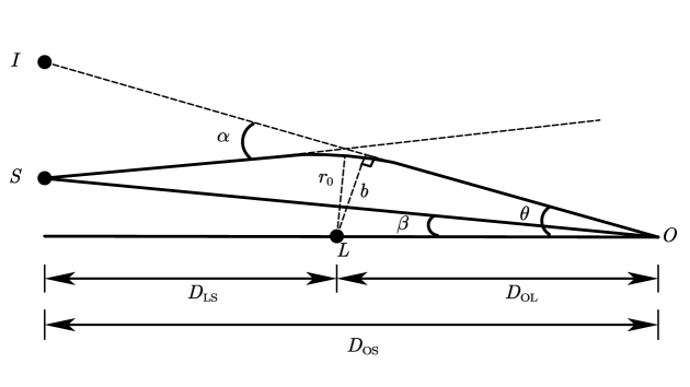
Figure 1: The fundamental geometric configuration underlying the phenomenon of gravitational lensing. $b$ is the impact parameter, $r_{0}$ represents the minimum distance between the light ray and the lens, and $I$ and $L$ denote the positions of the image and the lens. $S$ and $O$ represent the source and observer.

The image formed by photons that encircle a lens $n$ times is referred to as the $n$-th relativistic image. We consider the scenario when the source, lens, and observer are nearly perfectly aligned, which is precisely the condition under which relativistic imaging effects are most prominent. The angular position $\theta_{n}$ and magnification of the $n$-th image are given by Bozza et al. (2001); Bozza (2002)

$$\theta_{n}=\frac{b_{m}}{D_{\text{OL}}}(1+e_{n})=\theta_{\infty}(1+e_{n}),\quad e_{n}=e^{\frac{\bar{b}-2n\pi}{\bar{a}}},$$ (2.27)

$$\mu_{n}=e_{n}\frac{b_{m}^{2}\left(1+e_{n}\right)D_{\text{OS}}}{\bar{a}\beta D_{\text{OL}}^{2}D_{\text{LS}}},$$ (2.28)

where $\theta_{\infty}=b_{m}/D_{\text{OL}}$ designates the angular position where relativistic images are formed at the photon sphere.

It is hypothesized that the outermost (first) image in the series of images stands apart from the others, being uniquely discernible, while the remaining images nearly overlap and are difficult to distinguish. Therefore, we introduce an observable quantity: the angular separation, denoted as $s$, which quantifies the difference between the angular position of the first image and that of the subsequent ones. This quantity is defined as

$$s=\theta_{1}-\theta_{\infty}.$$ (2.29)

Furthermore, another observable is the ratio of the flux intensity of the primary image to the cumulative flux intensity of all subsequent images (hereafter abbreviated as the flux ratio). It is also known as the relative magnification. This ratio provides valuable insights into the relative brightness of the primary image compared to the collective contribution of the other images. It is given by

$$\mathcal{R}=\frac{\mu_{1}}{{\textstyle\sum_{n=2}^{\infty}}\mu_{n}},$$ (2.30)

where

$$\sum_{n=2}^{\infty}\mu_{n}=\frac{b_{m}^{2}D_{OS}}{\bar{a}\beta D_{OL}^{2}D_{LS}}\frac{e^{\frac{2\bar{b}-4\pi}{\bar{a}}}+e^{\frac{\bar{b}-2\pi}{\bar{a}}}+e^{\frac{\bar{b}}{\bar{a}}}}{e^{\frac{4\pi}{\bar{a}}}-1}.$$ (2.31)

After simplification, the flux ratio becomes

$$\mathcal{R}=\frac{(e^{\bar{b}/\bar{a}}+e^{2\pi/\bar{a}})(e^{4\pi/\bar{a}}-1)}{e^{\bar{b}/\bar{a}}+e^{2\pi/\bar{a}}+e^{4\pi/\bar{a}}}.$$ (2.32)

The detailed derivations of these observables can be found in Refs. Bozza et al. (2001); Bozza (2002).

III Gravitational lensing of RN black hole with a global monopole

We now investigate the gravitational lensing of an RN black hole with a global monopole. Its line element is given by Barriola and Vilenkin (1989); Guendelman and Rabinowitz (1991)

$$ds^{2}=-f(r)dt^{2}+\frac{1}{f(r)}dr^{2}+r^{2}d\theta^{2}+r^{2}\sin^{2}\theta d\varphi^{2},$$ (3.1)

where

$$f(r)=1-8\pi\gamma^{2}-\frac{2M}{r}+\frac{Q^{2}}{r^{2}}.$$ (3.2)

Here, $M$ and $Q$ represent the mass and charge of the black hole, respectively, and $\gamma$ is a parameter associated with the scale of gauge-symmetry breaking. The presence of a global monopole induces a deficit solid angle in spacetime, quantified by $\Delta=32\pi^{2}\gamma^{2}$ Barriola and Vilenkin (1989). This deficit angle modifies the geometry of spacetime, impacting the gravitational lensing properties.

For convenience, we introduce two dimensionless parameters to characterize the effects of the global monopole and charge: We define the global monopole parameter $\epsilon$ as

$$\epsilon=1-8\pi\gamma^{2}=1-\frac{\Delta}{4\pi},$$ (3.3)

which ranges from $\epsilon=0$ (corresponding to a maximum deficit solid angle $\Delta=4\pi$) to $\epsilon=1$ (when no monopole is present, i.e., $\Delta=0$), and the charge parameter $\eta$ as

$$\eta=Q^{2}/M^{2}.$$ (3.4)

This parameter quantifies the effect of charge, with values ranging from $\eta=0$ (uncharged black hole) to $\eta=1$ (extremal black hole in standard RN spacetime). To ensure that the spacetime does not develop a naked singularity, we impose the constraint $|Q|\leq M/\sqrt{\epsilon}$. For generality, and to avoid naked singularities for any $\epsilon$, we restrict the charge to $|Q|\leq M$, leading to the constraint $\eta\in[0,1]$. In the following sections, we analyze the gravitational lensing characteristics of this black hole spacetime and explore how the interplay between the charge and the global monopole affects lensing observables.

III.1 Physical quantities associated with gravitational lensing

In order to calculate the angular separation $s$ and the flux ratio $\mathcal{R}$ in the strong field limit using Eqs. (2.29) and (2.32), it is necessary to obtain the radius of the photon sphere $r_{m}$, the critical impact parameter $b_{m}$, the coefficients $\bar{a}$ and $\bar{b}$, and the regular integral $I_{R}$. These quantities are computed as follows.

From Eq. (2.5), the radius of the photon sphere $r_{m}$ is given by

$$r_{m}\left(\epsilon,\eta\right)=\bar{r}_{m}\left(\epsilon,\eta\right)M,$$ (3.5)

where

$$\bar{r}_{m}\left(\epsilon,\eta\right)=\frac{3+\sqrt{9-8\epsilon\eta}}{2}.$$ (3.6)

Meanwhile, the critical impact parameter $b_{m}$ can be obtained from Eq. (2.6) as

$$b_{m}\left(\epsilon,\eta\right)=\frac{\bar{r}_{m}^{2}\left(\epsilon,\eta\right)}{\sqrt{\epsilon\bar{r}_{m}^{2}\left(\epsilon,\eta\right)-2\bar{r}_{m}\left(\epsilon,\eta\right)+\eta}}M.$$ (3.7)

Based on Eqs. (2.24) and (2.25), the coefficients of the deflection angle $\bar{a}$ and $\bar{b}$ are derived as

$$\bar{a}\left(\epsilon,\eta\right)=\frac{\bar{r}_{m}\left(\epsilon,\eta\right)}{\sqrt{\epsilon\bar{r}_{m}^{2}\left(\epsilon,\eta\right)-2\eta}}$$ (3.8)

and

$$\bar{b}\left(\epsilon,\eta\right)=\bar{a}\left(\epsilon,\eta\right)\ln\left[\frac{6\bar{r}_{m}\left(\epsilon,\eta\right)-8\eta}{\bar{r}_{m}\left(\epsilon,\eta\right)-\eta}\right]+I_{R}\left(\bar{r}_{m}\right)-\pi,$$ (3.9)

respectively, where the regular integral $I_{R}$ can be obtained with Eq. (2.18) as

$$\begin{split}I_{R}\left(\bar{r}_{m}\right)&=\int_{0}^{1}{\frac{2\bar{r}_{m}}{z\sqrt{-\eta z^{2}-\left(2\bar{r}_{m}-4\eta\right)z+3\bar{r}_{m}+4\eta}}}-\frac{2\bar{a}}{z}dz\\ &=\bar{a}\ln\frac{4\left(3\bar{r}_{m}-4\eta\right)^{2}}{\left(2\bar{r}_{m}-2\eta+\sqrt{\bar{r}_{m}-\eta}\sqrt{3\bar{r}_{m}-4\eta}\right)^{2}},\end{split}$$ (3.10)

with $\bar{r}_{m}$ and $\bar{a}$ representing $\bar{r}_{m}(\epsilon,\eta)$ and $\bar{a}(\epsilon,\eta)$ for brevity. Thus, $\bar{b}$ is given by

$$\bar{b}(\epsilon,\eta)=\bar{a}(\epsilon,\eta)\ln\left[\frac{8\left(3\bar{r}_{m}(\epsilon,\eta)-4\eta\right)^{3}}{\bar{r}_{m}^{2}(\epsilon,\eta)\left(\bar{r}_{m}(\epsilon,\eta)-\eta\right)^{2}}\left(2\sqrt{\bar{r}_{m}(\epsilon,\eta)-\eta}-\sqrt{3\bar{r}_{m}(\epsilon,\eta)-4\eta}\right)^{2}\right]-\pi.$$ (3.11)

When the global monopole is absent ($\epsilon=1$), the coefficients $\bar{a}$ and $\bar{b}$ recover the results for the RN black hole, as derived in Ref. Tsukamoto (2017). Similarly, in the absence of charge ($\eta=0$), the coefficients $\bar{a}$ and $\bar{b}$ reduce to the expressions obtained for a Schwarzschild black hole with a global monopole, as given in Ref. Cheng and Man (2011). Furthermore, in the absence of both charge and the global monopole ($\eta=0$, $\epsilon=1$), the coefficients $\bar{a}$ and $\bar{b}$ match the results from Refs. Bozza (2002); Tsukamoto (2017) for a Schwarzschild black hole. These consistency checks further validate our approach, ensuring that the inclusion of both charge and a global monopole provides a unified framework that naturally extends existing results.

III.2 Typical observables in gravitational lensing

By leveraging the coefficients $\bar{a}$ and $\bar{b}$ of the deflection angle, we now derive explicit analytical expressions for the angular separation $s$ and the flux ratio $\mathcal{R}$ using Eqs. (2.29) and (2.32). Previous studies have primarily relied on numerical approaches to analyze these observables in specific scenarios. For instance: Ref. Bozza (2002) conducted numerical computations for an RN black hole, but did not provide analytical formulas for $s$ and $\mathcal{R}$. Ref. Cheng and Man (2011) focused on a Schwarzschild black hole with a global monopole, again without explicit analytical expressions for the observables. In this work, we go beyond previous studies by deriving explicit analytical expressions for both $s$ and $\mathcal{R}$ for an RN black hole with a global monopole, facilitating a direct evaluation of how these observables respond to variations in charge ($\eta$) and the global monopole parameter ($\epsilon$). To achieve a comprehensive understanding, we conduct both analytical and numerical analyses, examining both the individual effects of the global monopole and charge on the observables, as well as the combined impact of charge and the global monopole, revealing their interplay in modifying strong-field lensing behavior.

III.2.1 The angular separation

The angular separation between the first image and the subsequent images can be obtained using Eq. (2.29) as

$$s(\epsilon,\eta)= \frac{M}{D_{\text{OL}}\sqrt{\epsilon\bar{r}_{m}^{2}-2\bar{r}_{m}+\eta}}\left[\frac{8\left(3\bar{r}_{m}-4\eta\right)^{3}}{\left(\bar{r}_{m}-\eta\right)^{2}}\right]\left(2\sqrt{\bar{r}_{m}-\eta}-\sqrt{3\bar{r}_{m}-4\eta}\right)^{2}\exp\left(\frac{-3\pi\sqrt{\epsilon\bar{r}_{m}^{2}-2\eta}}{\bar{r}_{m}}\right),$$ (3.12)

where $\bar{r}_{m}$ represents $\bar{r}_{m}(\epsilon,\eta)$ for brevity.

Firstly, we examine the dependence of the angular separation on the global monopole parameter for a fixed charge. When the charge vanishes ($\eta=0$), the angular separation is given by

$$s(\epsilon,0)=\frac{648\sqrt{3}\left(2-\sqrt{3}\right)^{2}M}{D_{\text{OL}}\epsilon^{3/2}}e^{-3\pi\sqrt{\epsilon}}.$$ (3.13)

It is evident that the angular separation $s$ increases as the global monopole parameter $\epsilon$ decreases (i.e., as the deficit solid angle $\Delta$ caused by the global monopole increases). This means that the presence of a global monopole results in a larger angular separation between the first image and the subsequent images, which is consistent with the numerical results in Ref. Cheng and Man (2011). When the charge is nonzero, the analytical expression becomes more complex. However, it is direct to check numerically that the partial derivative of the angular separation $s$ with respect to the global monopole parameter $\epsilon$ in the region $\epsilon\in[0,1]$ and $\eta\in[0,1]$ is always negative, meaning that the angular separation always increases as the deficit solid angle $\Delta$ caused by the global monopole increases, regardless of whether the black hole is charged or not.

Secondly, we investigate the dependence of the angular separation on the charge for a fixed global monopole parameter. First, when there is charge but no global monopole (i.e., $\epsilon=1$), the angular separation is given by the expression:

$$s(1,\eta)=\frac{M}{D_{\text{OL}}\sqrt{w^{2}-2w+\eta}}\left[\frac{8\left(3w-4\eta\right)^{3}}{\left(w-\eta\right)^{2}}\right]\left(2\sqrt{w-\eta}-\sqrt{3w-4\eta}\right)^{2}\exp\left(\frac{-3\pi\sqrt{w^{2}-2\eta}}{w}\right),$$ (3.14)

where $w$ represents the dimensionless radius of the photon sphere, $\bar{r}_{m}(1,\eta)$. Furthermore, as shown in Appendix A, the derivative of the angular separation with respect to $\eta$ is always positive. This indicates that the angular separation monotonically increases with increasing charge. Now, we analyze the behavior of the angular separation $s$ in the presence of both charge and a global monopole. Directly analyzing Eq. (3.12) is challenging due to its complexity. To understand the effects of both charge and the global monopole, we expand the angular separation expression for small and large charge values, respectively. For small charge ($\eta\ll 1$), Eq. (3.12) can be expanded as

$$s=\frac{648\left(7\sqrt{3}-12\right)e^{-3\pi\sqrt{\epsilon}}M}{\epsilon^{3/2}D_{OL}}+\frac{108\left[2\pi\left(7\sqrt{3}-12\right)\sqrt{\epsilon}-51\sqrt{3}+88\right]e^{-3\pi\sqrt{\epsilon}}M}{\sqrt{\epsilon}D_{OL}}\eta+\mathcal{O}\left(\eta^{2}\right).$$ (3.15)

The dependence of the angular separation on charge is determined by the coefficient of the $\eta$-dependent term. There exists a critical value of the global monopole parameter, given by $\epsilon_{0}=\left[\frac{51\sqrt{3}-88}{2\pi\left(7\sqrt{3}-12\right)}\right]^{2}\approx 0.1833742$, which separates two behaviors: For $\epsilon>\epsilon_{0}$, coefficient of the $\eta$-dependent term is positive, and the angular separation increases with charge. Conversely, for $\epsilon<\epsilon_{0}$, the coefficient is negative, and the angular separation decreases with charge. For large charge ($\eta\to 1$), the angular separation (Eq. (3.12)) behaves as:

$$s=H\left(\epsilon\right)+F\left(\epsilon\right)\left(1-\eta\right)+\mathcal{O}\left((1-\eta)^{2}\right),$$ (3.16)

where $H(\epsilon)$ and $F(\epsilon)$ are functions of the global monopole parameter $\epsilon$. Due to the complexity of these expressions, their explicit forms are provided in Appendix B. We find that, similar to the small-charge case, there exists a critical value $\epsilon_{1}\approx 0.1826688$, above which $F(\epsilon)$ is negative and the angular separation increases with charge, and below which $F(\epsilon)$ is positive and the angular separation decreases with charge. The analysis reveals that the global monopole parameter introduces a non-monotonic behavior in the angular separation with respect to charge. There are critical values of $\epsilon$ ($\epsilon_{0}$ and $\epsilon_{1}$) that determine whether the angular separation increases or decreases with charge. This behavior is distinctly different from the RN black hole case, where the angular separation always increases with charge.

The analysis above focuses on the monotonicity of the angular separation in the small-charge ($\eta\to 0$) and large-charge ($\eta\to 1$) limits. To gain a more comprehensive understanding of its behavior for arbitrary black hole charge, we examine numerically the sign of the partial derivative of the angular separation $s$ with respect to the charge parameter $\eta$ as a function of the global monopole parameter $\epsilon$ and the charge parameter $\eta$, as shown in Fig. 2. Additionally, Figs. 22(b) and 22(c) provide enlarged views of specific regions of Fig. 2(a). The figures clearly reveal that, in addition to the two critical values $\epsilon_{0}$ and $\epsilon_{1}$ found in the analytical investigation, a third critical value $\epsilon_{2}\approx 0.1826576$ emerges from the numerical analysis. These critical points divide the parameter space into four distinct regions that govern the monotonicity and behavior of the angular separation $s$ with respect to the charge parameter ($\eta$): 1. When $\epsilon<\epsilon_{2}$, the partial derivative is always negative, indicating that the angular separation decreases monotonically with charge. 2. When $\epsilon_{2}<\epsilon<\epsilon_{1}$, the angular separation initially decreases, then increases, and subsequently decreases again as the charge increases. This non-monotonic behavior results in the angular separation exhibiting both a minimum and a maximum, as illustrated in Fig. 3. 3. When $\epsilon_{1}<\epsilon<\epsilon_{0}$, the angular separation initially decreases and then increases as the charge increases. This again indicates the existence of a single minimum in the angular separation as a function of charge, as demonstrated in Fig. 3. 4. When $\epsilon>\epsilon_{0}$, the partial derivative is always positive, meaning that the angular separation increases monotonically with charge. These results reveal that the presence of the global monopole introduces more complex behavior in the angular separation as a function of charge. In particular, the angular separation does not always increase with charge, as it does for the RN black hole. Instead, the behavior depends on the global monopole parameter $\epsilon$, with some regions exhibiting a minimum or maximum angular separation as charge varies.

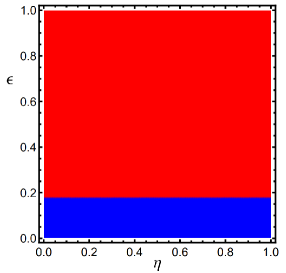
(a)

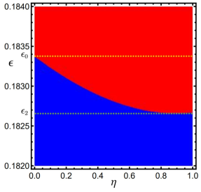
(b)

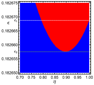
(c)

Figure 2: (a) The sign of the first-order partial derivative of the angular separation $s$ with respect to the charge parameter $\eta$, where positive values are shown in red and negative values in blue. (b) An enlarged view of Fig. 2(a) in the region $\epsilon\in\left[0.182,0.184\right]$. (c) An enlarged view of Fig. 2(a) in the region $\epsilon\in\left[0.182650,0.182675\right]$ and $\eta\in\left[0.7,1\right]$. The yellow, white, and green dashed lines correspond to the critical values $\epsilon_{0}\approx 0.1833742$, $\epsilon_{1}\approx 0.1826688$, and $\epsilon_{2}\approx 0.1826576$, respectively.

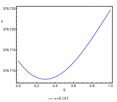
(a)

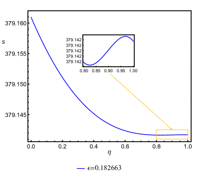
(b)

Figure 3: (a) The dependence of angular separation $s$ on the charge parameter $\eta$ when $\epsilon=0.183$, where $\epsilon_{1}<\epsilon<\epsilon_{0}$. (b) The dependence of angular separation $s$ on the charge parameter $\eta$ when $\epsilon=0.182663$, where $\epsilon_{2}<\epsilon<\epsilon_{1}$. In both cases, the angular separation is measured in microarc sec, and $D_{\text{OL}}=10^{10}M$.

III.2.2 The flux ratio

The flux ratio is given by Eq. (2.32) as

$$\mathcal{R}(\epsilon,\eta)=\frac{(e^{\bar{b}/\bar{a}}+e^{2\pi/\bar{a}})(e^{4\pi/\bar{a}}-1)}{e^{\bar{b}/\bar{a}}+e^{2\pi/\bar{a}}+e^{4\pi/\bar{a}}},$$ (3.17)

where $\bar{a}$ and $\bar{b}$ denote $\bar{a}(\epsilon,\eta)$ and $\bar{b}(\epsilon,\eta)$, respectively. Direct analysis of the dependence of the flux ratio in Eq. (3.17) on the charge and the global monopole parameter is complex. To gain a more intuitive understanding of the influence of the global monopole on the flux ratio, we focus on the case where the deficit angle caused by the global monopole is small, i.e., when $\epsilon$ is close to $1$. In this scenario, $e^{\frac{2\pi}{\bar{a}}}\gg e^{\frac{\bar{b}}{\bar{a}}}$, and thus Eq. (3.17) can be approximated as

$$\mathcal{R}(\epsilon,\eta)\approx e^{\frac{2\pi}{\bar{a}}}=\exp\left[\frac{2\pi\sqrt{\epsilon\bar{r}_{m}^{2}-2\eta}}{\bar{r}_{m}}\right],$$ (3.18)

where $\bar{r}_{m}$ represents $\bar{r}_{m}(\epsilon,\eta)$.

First, we investigate the dependence of the flux ratio $\mathcal{R}$ on the charge parameter $\eta$ for a fixed global monopole parameter $\epsilon$. From Eq. (3.18), we obtain

$$\frac{\partial\mathcal{R}}{\partial\eta}=-\frac{6\pi}{\left[\bar{r}_{m}K\left(\epsilon,\eta\right)\right]^{\frac{3}{2}}}\exp\left(2\pi\sqrt{\frac{K\left(\epsilon,\eta\right)}{\bar{r}_{m}}}\right)<0,$$ (3.19)

where $K\left(\epsilon,\eta\right)=\sqrt{9-8\epsilon\eta}$. Therefore, the flux ratio $\mathcal{R}$ decreases monotonically as the charge increases when the deficit solid angle induced by the global monopole is small (i.e., when $\epsilon$ is close to 1). Furthermore, we numerically investigate the partial derivative of the flux ratio $\mathcal{R}$ (3.17) with respect to the charge parameter $\eta$, which is always negative in the region $\epsilon\in[0,1]$ and $\eta\in[0,1]$. This indicates that the flux ratio $\mathcal{R}$ decreases monotonically with $\eta$, irrespective of the value of the global monopole parameter $\epsilon$.

Next, we analyze how the flux ratio $\mathcal{R}$ varies with the global monopole parameter $\epsilon$ for a fixed charge. For $\epsilon$ close to $1$, Eq. (3.18) can be expanded as

$$\mathcal{R}=\exp\left[2\pi\sqrt{\frac{2W(\eta)}{G\left(\eta\right)}}\right]+\frac{2\sqrt{2}\pi I\left(\eta\right)}{G^{\frac{3}{2}}\left(\eta\right)W(\eta)}\exp\left[2\pi\sqrt{\frac{2W(\eta)}{G\left(\eta\right)}}\right]\left(1-\epsilon\right)+\mathcal{O}\left((1-\epsilon)^{2}\right),$$ (3.20)

where $W(\eta)=\sqrt{9-8\eta}$, $G\left(\eta\right)=3+\sqrt{9-8\eta}$, and

$$I\left(\eta\right)=-32\eta^{2}+6\left(5\sqrt{9-8\eta}+21\right)\eta-27\left(\sqrt{9-8\eta}+3\right).$$ (3.21)

The sign of $I(\eta)$ determines whether the flux ratio $\mathcal{R}$ increases or decreases with the global monopole parameter $\epsilon$. From the above equations, we find a critical value $\eta_{0}=\frac{27}{32}$ (or equivalently, a critical charge $Q_{0}=\frac{3\sqrt{6}}{8}M$) such that $I(\eta_{0})=0$. Specifically, the flux ratio $\mathcal{R}$ increases with $\epsilon$ (i.e., decreases with the deficit angle) when $\eta<\eta_{0}$, whereas $\mathcal{R}$ decreases as $\epsilon$ increases (i.e., as the deficit angle decreases) when $\eta>\eta_{0}$. This behavior is in sharp contrast to the case without charge, where the flux ratio increases monotonically with the global monopole parameter, or as the deficit angle decreases, as demonstrated numerically in Ref. Cheng and Man (2011).

We now numerically analyze the behavior of the flux ratio $\mathcal{R}$ over a broader parameter range. As shown in Fig. 4, the critical value $\eta_{0}=\frac{27}{32}\approx 0.84$ (indicated by the yellow dashed line) divides the parameter space into two distinct regions. When the charge parameter $\eta$ is less than $\eta_{0}$, the flux ratio $\mathcal{R}$ decreases monotonically with the global monopole parameter $\epsilon$. In contrast, when $\eta$ exceeds $\eta_{0}$, the flux ratio $\mathcal{R}$ initially increases and then decreases as $\epsilon$ increases. To illustrate these behaviors explicitly, we show the flux ratio as a function of the global monopole parameter $\epsilon$ for a fixed charge in Fig. 5. From this figure, we observe that when the charge satisfies $\eta\leq\frac{27}{32}$ (i.e., the red and black lines), the flux ratio $\mathcal{R}$ increases as the global monopole parameter $\epsilon$ increases (i.e., as the deficit angle decreases). However, when $\eta>\eta_{0}$ (i.e., the blue line), the flux ratio $\mathcal{R}$ initially increases and then decreases. Additionally, it can also be seen from Fig. 5 that, when the global monopole parameter $\epsilon$ is fixed, the flux ratio $\mathcal{R}$ decreases as the charge (i.e., the parameter $\eta$) increases.

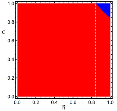
Figure 4: The sign of the first-order partial derivative of the flux ratio $\mathcal{R}$ with respect to the global monopole parameter $\epsilon$, where positive values are shown in red and negative values in blue. The yellow line represents the critical charge paremeter $\eta_{0}$.

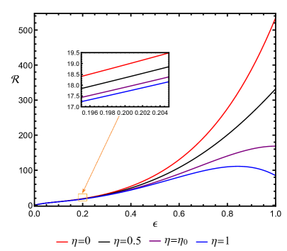
Figure 5: The dependence of flux ratio $\mathcal{R}$ on the deficit angle characterized by $\epsilon$ for fixed charge. The solid red, black, purple, and blue lines correspond to charge parameter $\eta=Q^{2}/M^{2}$ with values of $0$, $0.5$, $\eta_{0}$, and $1$, respectively. The inset shows an enlargement of the interval $\epsilon\in[0.195,0.205]$.

IV Discussion

In this paper, we have investigated the gravitational lensing near a charged black hole with a global monopole in the strong field limit, focusing on the interplay between charge and the global monopole on lensing observables. Notably, the phenomena described here, such as the non-monotonic behavior of the angular separation, are particularly intriguing when both charge and the global monopole’s deficit angle are large, with critical values identified for both parameters (refer to the critical values for $\eta$ and $\epsilon$ in the last section). However, astrophysical black holes are expected to be nearly neutral, as any significant charge would likely be neutralized by surrounding matter. Furthermore, the deficit angle caused by a global monopole is expected to be extremely small. In typical grand unification scenarios, the parameter $\gamma$ in the metric (3.1) characterizing the global monopole is on the order of $\sim 10^{16}$ GeV Barriola and Vilenkin (1989), leading to a deficit angle $\Delta=32\pi^{2}\gamma^{2}\sim 4\pi\times 10^{-5}$ rad, which is negligibly small. Consequently, the phenomena described in this paper are unlikely to be observed in typical astrophysical black holes.

Nevertheless, there is growing interest in analogue gravity systems Barcelo et al. (2005) as platforms for studying gravitational effects, particularly gravitational lensing Fischer and Visser (2002); Sheng et al. (2013). These systems, which use acoustic, optical, or other artificial materials to mimic the behavior of spacetime, allow for more flexibility in tuning parameters such as charge and deficit angle, which may be too small in natural systems. In particular, the theory of transformation optics Leonhardt (2006); Pendry et al. (2006) establishes a correspondence between the metric tensor and the permittivity and permeability tensors of materials, enabling the design of optical metamaterials to mimic astronomical phenomena. For instance, gravitational lensing effects have been experimentally visualized in such systems Sheng et al. (2013). In such optical metamaterials, the effective charge and deficit angle are not constrained to be small. In particular, by using an artificial waveguide bounded with rotational metasurface, the nontrivial effects of a spacetime topological defect have been experimentally emulated, and photon deflection in the topological waveguide has been observed Sheng et al. (2018). In this context, the phenomena predicted here may potentially be observed in analogue systems.

V Conclusion

In this paper, we have investigated the phenomenon of gravitational lensing near a charged black hole with a global monopole, with particular focus on the effects of the black hole charge and the global monopole on key lensing observables. We have derived the coefficients $\bar{a}$ and $\bar{b}$ that characterize the deflection angle of light. Based on these results, we have investigated the effects of the global monopole and the black hole charge on two key observables in gravitational lensing: the angular separation $s$ between the first image and subsequent images, and the flux ratio $\mathcal{R}$, defined as the ratio of the flux intensity from the first image to the cumulative flux intensity of all other images. We have derived analytical expressions for the observables $s$ and $\mathcal{R}$, and performed both analytical and numerical analyses. The findings are summarized as follows:

For the angular separation $s$, we find that regardless of the value of the charge, $s$ always decreases as the deficit angle caused by the global monopole decreases. However, the behavior of $s$ as a function of the charge is highly dependent on the global monopole parameter. We identified three critical values of the global monopole parameter, which divide the parameter space into four distinct regions. In these regions, the angular separation $s$ can either increase or decrease monotonically with charge, or exhibit more complex behaviors such as an initial decrease followed by an increase, or a non-monotonic behavior with both a maximum and a minimum. These behaviors contrast sharply with the monotonic increase in angular separation as a function of charge observed in the absence of a global monopole.

For the flux ratio $\mathcal{R}$, we find that irrespective of the global monopole parameter, $\mathcal{R}$ always decreases as the charge increases. However, the dependence of $\mathcal{R}$ on the global monopole parameter, or the deficit angle, varies with the charge $Q$. A critical charge $Q_{0}$ exists such that when the charge is smaller than this critical value, $\mathcal{R}$ increases as the deficit angle caused by the global monopole decreases. In contrast, when the charge exceeds the critical value, $\mathcal{R}$ initially increases and then decreases with decreasing deficit angle, exhibiting a maximum value. This behavior also differs from the monotonically decreasing flux ratio as the deficit angle increases in the absence of charge.

These results demonstrate that in the strong field limit, the charge and global monopole interact in complex ways, and their combined effects on the lensing observables cannot be attributed to the independent contributions of each factor. The resulting lensing signatures provide a rich landscape for further exploration.

While the charge and global monopole deficit angle are expected to be small in typical astrophysical black holes, these parameters are not constrained in analogue gravity systems. Therefore, the phenomena predicted here, including the non-monotonic behavior of the angular separation and flux ratio, may potentially be observed in optical metamaterials or other experimental setups designed to mimic black hole physics. These findings open up new avenues for testing gravitational lensing effects in laboratory-based systems, offering the possibility of future experimental verification of our theoretical predictions.

Appendix A The derivative of angular separation with respect to $\eta$

$s(1,\eta)$ is given by:

$$s\left(1,\eta\right)=\frac{M}{D_{\text{OL}}\sqrt{w^{2}-2w+\eta}}\left[\frac{8\left(3w-4\eta\right)^{3}}{\left(w-\eta\right)^{2}}\right]\left(2\sqrt{w-\eta}-\sqrt{3w-4\eta}\right)^{2}\exp\left(\frac{-3\pi\sqrt{w^{2}-2\eta}}{w}\right),$$ (1)

where

$$w=\frac{3+\sqrt{9-8\eta}}{2}.$$ (2)

Taking the logarithmic derivative of $s(1,\eta)$, we obtain

$$\begin{split}\tilde{s}(\eta):=\frac{D_{\text{OL}}}{8M}\frac{d\ln s(1,\eta)}{d\eta}=&\frac{\left(16\eta+4w+4\sqrt{w-\eta}\sqrt{3w-4\eta}-33\right)}{2(\eta-1)(8\eta-9)}\\ &+\frac{\left(4\sqrt{3w-4\eta}\sqrt{w-\eta}-9\right)\left(w-3\right)}{2\eta(\eta-1)(8\eta-9)}\\ &-\frac{18\sqrt{2}\pi\left[2\left(2w+3\right)\eta-9w\right]}{w^{2}\left(6w-8\eta\right)^{3/2}(2w-3)}\end{split}$$ (3)

The trend of $\tilde{s}$ changing with $\eta$ is shown in the Fig. 6. Obviously, $\tilde{s}(\eta)$ is always positive.

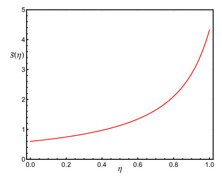
Figure 6: The behavior of $\tilde{s}(\eta)$ with $\eta$.

Appendix B Explicit expressions for $H(\epsilon)$ and $F(\epsilon)$ in Eq. (3.16)

In this appendix, we provide the explicit expressions for $H(\epsilon)$ and $F(\epsilon)$ in Eq. (3.16). For convenience, we define the following three functions:

$$h\left(\epsilon\right)=\sqrt{9-8\epsilon},$$ (1)

$$f_{1}\left(\epsilon\right)=3+\sqrt{9-8\epsilon},$$ (2)

and

$$f_{2}\left(\epsilon\right)=\sqrt{f_{1}\left(\epsilon\right)-2\epsilon}.$$ (3)

The function $H(\epsilon)$ is given by

$$H\left(\epsilon\right)=\frac{2\sqrt{2}}{f_{2}\left(\epsilon\right)^{5}\epsilon^{3/2}}\left[f_{1}\left(\epsilon\right)h\left(\epsilon\right)\right]^{3}\left[\sqrt{f_{1}\left(\epsilon\right)h\left(\epsilon\right)}-2f_{2}\left(\epsilon\right)\right]^{2}\exp\left[3\sqrt{2}\pi\sqrt{\frac{\epsilon h\left(\epsilon\right)}{f_{1}\left(\epsilon\right)}}\right],$$ (4)

and the function $F(\epsilon)$ takes the form

$$F\left(\epsilon\right)=-\frac{2\left[\sqrt{f_{1}\left(\epsilon\right)h\left(\epsilon\right)}-2f_{2}\left(\epsilon\right)\right]}{\left[f_{1}\left(\epsilon\right)h\left(\epsilon\right)\right]^{\frac{3}{2}}f_{2}\left(\epsilon\right)^{7}\epsilon^{7/2}}\left[N_{1}\left(\epsilon\right)+N_{2}\left(\epsilon\right)\right]\exp\left[3\sqrt{2}\pi\sqrt{\frac{\epsilon h\left(\epsilon\right)}{f_{1}\left(\epsilon\right)}}\right],$$ (5)

where

$$N_{1}\left(\epsilon\right)=4\epsilon^{3}h\left(\epsilon\right)^{3}f_{1}\left(\epsilon\right)^{4}f_{2}\left(\epsilon\right)\left[\left(h\left(\epsilon\right)+2\right)\sqrt{f_{1}\left(\epsilon\right)h\left(\epsilon\right)}-\left(2h\left(\epsilon\right)+3\right)f_{2}\left(\epsilon\right)\right],$$ (6)

and

$$\begin{split}N_{2}\left(\epsilon\right)=&36\pi\sqrt{2}\epsilon^{7/2}\left[\sqrt{f_{1}\left(\epsilon\right)h\left(\epsilon\right)}-2f_{2}\left(\epsilon\right)\right]\left[8\epsilon^{2}-\left(7h\left(\epsilon\right)+33\right)\epsilon+9f_{1}\left(\epsilon\right)\right]\left[f_{1}\left(\epsilon\right)h\left(\epsilon\right)\right]^{2}\\ &+2\epsilon^{3}\left[\sqrt{f_{1}\left(\epsilon\right)h\left(\epsilon\right)}-2f_{2}\left(\epsilon\right)\right]\left[-32\epsilon^{2}+44\left(h\left(\epsilon\right)+6\right)\epsilon-99f_{1}\left(\epsilon\right)\right]\left[f_{1}\left(\epsilon\right)h\left(\epsilon\right)\right]^{5/2}.\end{split}$$ (7)

The numerical solution of $F(\epsilon_{1})=0$ gives $\epsilon_{1}\approx 0.1826688$. To illustrate the behavior of $F(\epsilon)$ around $\epsilon_{1}$, we present a plot of $F(\epsilon)$ in Fig. 7. From Fig. 7, it is evident that $F(\epsilon)>0$ when $\epsilon<\epsilon_{1}$, while $F(\epsilon)<0$ when $\epsilon>\epsilon_{1}$.

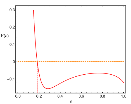
Figure 7: $F(\epsilon)$ as a function of the global monopole parameter $\epsilon$. The abscissa of the zero point of the function is $\epsilon_{1}$.

References

- Einstein (1936) A. Einstein, Science 84, 506 (1936).
- Walsh et al. (1979) D. Walsh, R. F. Carswell, and R. J. Weymann, Nature 279, 381 (1979).
- Virbhadra and Ellis (2000) K. S. Virbhadra and G. F. R. Ellis, Phys. Rev. D 62, 084003 (2000), arXiv:astro-ph/9904193 .
- Bozza et al. (2001) V. Bozza, S. Capozziello, G. Iovane, and G. Scarpetta, Gen. Rel. Grav. 33, 1535 (2001), arXiv:gr-qc/0102068 .
- Bozza (2002) V. Bozza, Phys. Rev. D 66, 103001 (2002), arXiv:gr-qc/0208075 .
- Tsukamoto (2017) N. Tsukamoto, Phys. Rev. D 95, 064035 (2017), arXiv:1612.08251 [gr-qc] .
- Bozza (2003) V. Bozza, Phys. Rev. D 67, 103006 (2003), arXiv:gr-qc/0210109 .
- Bozza et al. (2006) V. Bozza, F. De Luca, and G. Scarpetta, Phys. Rev. D 74, 063001 (2006), arXiv:gr-qc/0604093 .
- Bozza et al. (2005) V. Bozza, F. De Luca, G. Scarpetta, and M. Sereno, Phys. Rev. D 72, 083003 (2005), arXiv:gr-qc/0507137 .
- Hsieh et al. (2021) T. Hsieh, D.-S. Lee, and C.-Y. Lin, Phys. Rev. D 103, 104063 (2021), arXiv:2101.09008 [gr-qc] .
- Chen et al. (2025) B.-R. Chen, T. Hsieh, and D.-S. Lee, Phys. Rev. D 111, 024058 (2025), arXiv:2411.00458 [gr-qc] .
- Eiroa (2005) E. F. Eiroa, Phys. Rev. D 71, 083010 (2005), arXiv:gr-qc/0410128 .
- Whisker (2005) R. Whisker, Phys. Rev. D 71, 064004 (2005), arXiv:astro-ph/0411786 .
- Tsukamoto et al. (2012) N. Tsukamoto, T. Harada, and K. Yajima, Phys. Rev. D 86, 104062 (2012), arXiv:1207.0047 [gr-qc] .
- Tsukamoto (2016) N. Tsukamoto, Phys. Rev. D 94, 124001 (2016), arXiv:1607.07022 [gr-qc] .
- Gyulchev and Yazadjiev (2007) G. N. Gyulchev and S. S. Yazadjiev, Phys. Rev. D 75, 023006 (2007), arXiv:gr-qc/0611110 .
- Tsukamoto (2021a) N. Tsukamoto, Phys. Rev. D 103, 024033 (2021a), arXiv:2011.03932 [gr-qc] .
- Tsukamoto (2021b) N. Tsukamoto, Phys. Rev. D 104, 064022 (2021b), arXiv:2105.14336 [gr-qc] .
- Chagoya et al. (2021) J. Chagoya, C. Ortiz, B. Rodríguez, and A. A. Roque, Class. Quant. Grav. 38, 075026 (2021), arXiv:2007.09473 [gr-qc] .
- Younas et al. (2015) A. Younas, S. Hussain, M. Jamil, and S. Bahamonde, Phys. Rev. D 92, 084042 (2015), arXiv:1502.01676 [gr-qc] .
- Vachher et al. (2024) A. Vachher, D. Baboolal, and S. G. Ghosh, Phys. Dark Univ. 44, 101493 (2024).
- Virbhadra and Ellis (2002) K. S. Virbhadra and G. F. R. Ellis, Phys. Rev. D 65, 103004 (2002).
- Soares et al. (2023) A. R. Soares, C. F. S. Pereira, R. L. L. Vitória, and E. M. Rocha, Phys. Rev. D 108, 124024 (2023), arXiv:2309.05106 [gr-qc] .
- Cheng and Man (2011) H. Cheng and J. Man, Class. Quant. Grav. 28, 015001 (2011), arXiv:1004.3423 [hep-th] .
- Man and Cheng (2015) J. Man and H. Cheng, Phys. Rev. D 92, 024004 (2015), arXiv:1205.4857 [gr-qc] .
- Soares et al. (2024) A. R. Soares, R. L. L. Vitória, and C. F. S. Pereira, Phys. Rev. D 110, 084004 (2024), arXiv:2408.03217 [gr-qc] .
- Barriola and Vilenkin (1989) M. Barriola and A. Vilenkin, Phys. Rev. Lett. 63, 341 (1989).
- Yu (1994) H.-W. Yu, Nucl. Phys. B 430, 427 (1994).
- Barcelo et al. (2005) C. Barcelo, S. Liberati, and M. Visser, Living Rev. Rel. 8, 12 (2005), arXiv:gr-qc/0505065 .
- Guendelman and Rabinowitz (1991) E. I. Guendelman and A. Rabinowitz, Phys. Rev. D 44, 3152 (1991).
- Fischer and Visser (2002) U. R. Fischer and M. Visser, Phys. Rev. Lett. 88, 110201 (2002), arXiv:cond-mat/0110211 .
- Sheng et al. (2013) C. Sheng, H. Liu, Y. Wang, S. N. Zhu, and D. A. Genov, Nature Photonics 7, 902 (2013).
- Leonhardt (2006) U. Leonhardt, Science 312, 1777 (2006).
- Pendry et al. (2006) J. B. Pendry, D. Schurig, and D. R. Smith, Science 312, 1780 (2006).
- Sheng et al. (2018) C. Sheng, H. Liu, H. Chen, and S. Zhu, Nature Commun. 9, 4271 (2018), arXiv:1810.06280 [physics.optics] .