Revealing Bias Formation in Deep Neural Networks Through the Geometric Mechanisms of Human Visual Decoupling

Abstract

Deep neural networks (DNNs) often exhibit biases toward certain categories during object recognition, even under balanced training data conditions. The intrinsic mechanisms underlying these biases remain unclear. Inspired by the human visual system, which decouples object manifolds through hierarchical processing to achieve object recognition, we propose a geometric analysis framework linking the geometric complexity of class-specific perceptual manifolds in DNNs to model bias. Our findings reveal that differences in geometric complexity can lead to varying recognition capabilities across categories, introducing biases. To support this analysis, we present the Perceptual-Manifold-Geometry library, designed for calculating the geometric properties of perceptual manifolds.

Bias formation in deep neural networks (DNNs) remains a critical yet poorly understood challenge, influencing both fairness and reliability in artificial intelligence systems. While previous studies have primarily focused on statistical imbalances in training data, recent advances suggest that the intrinsic geometry of feature representations may play a fundamental role in shaping classification biases. Motivated by findings in cognitive science and geometric deep learning, this study introduces a theoretical framework to analyze how perceptual manifold geometry affects class-wise recognition performance. By quantifying manifold complexity through curvature, dimensionality, and topological measures, this work reveals a strong correlation between geometric structure and classification bias. These findings contribute to a deeper theoretical foundation for understanding chaos and complexity in modern learning systems, offering new perspectives at the intersection of machine learning, neuroscience, and nonlinear dynamics.

I Introduction

Deep neural networks (DNNs), with their powerful learning and generalization capabilities, have been widely applied in visual tasks such as image classification and object detection Chiu et al. (2024); Li et al. (2022). However, the biases exhibited by DNNs toward different categories significantly limit their fairness and reliability in real-world applications Jiang et al. (2022); Hu et al. (2024). Traditional theories mainly attribute these biases to the long-tailed distribution of training samples Yang et al. (2022); Alshammari et al. (2022). Nonetheless, research and practical observations suggest that even with balanced datasets, DNNs still show substantially better recognition performance for certain categories over others Ma et al. (2023a); Kaushik et al. (2024). This indicates that the mechanisms underlying such biases are more complex and remain poorly understood.

The human visual system provides critical insights into understanding the origins of biases in DNNs. When neurons in the visual cortex are stimulated by different physical attributes of objects belonging to the same category, they form Object manifolds Langdon, Genkin, and Engel (2023); DiCarlo and Cox (2007). As shown in Figure.1a, the human visual cortex gradually disentangles and reduces the dimensionality of complex Object manifolds layer by layer, making them easier to distinguish in deeper cortical areas, thereby achieving object recognition DiCarlo and Cox (2007); Peelen, Berlot, and de Lange (2024). This process suggests that the geometric complexity of Object manifolds influences the difficulty of disentanglement and recognition performance DiCarlo and Cox (2007); Li and Wang (2023); Chong and Feng (2024).

Considering that the architecture of DNNs mimics this multi-layer disentanglement mechanism Krizhevsky, Sutskever, and Hinton (2012); Bollt (2024), and recent studies Ma et al. (2023b); Cohen et al. (2020); Greco and Siegel (2024) demonstrate that the responses of DNNs to images exhibit manifold-like properties similar to those of the human visual system, we refer to the point-cloud manifolds formed by the embeddings of data in the feature space of a trained DNN’s representation network as class-specific perceptual manifolds. Formally, given a dataset $X=[x_{1},\dots,x_{m}]$ belonging to a specific class and a trained deep neural network $\text{Model}=\{f(x,\theta_{1}),g(z,\theta_{2})\}$, where $f(x,\theta_{1})$ represents the representation network and $g(z,\theta_{2})$ denotes the classifier, we extract the $p$-dimensional embeddings $Z=[z_{1},\dots,z_{m}]\in\mathbb{R}^{p\times m}$ using the representation network, with each $z_{i}=f(x_{i},\theta_{1})\in\mathbb{R}^{p}$. The point-cloud manifold formed by $Z$ is referred to as the class-specific perceptual manifold within the DNN. If the recognition process of DNNs can be viewed as the representation network disentangling, reducing the dimensionality of, and separating class-specific perceptual manifolds, followed by the classifier making decisions (as illustrated in Figure.1b), we hypothesize that: (1) The higher the geometric complexity of a class-specific perceptual manifold produced by the representation network, the more challenging it becomes for the classifier to decode and recognize the corresponding class. (2) Differences in geometric complexity across classes lead to inconsistent recognition capabilities, thus introducing biases.

Results

To validate this hypothesis, we conducted experiments on widely used image datasets with balanced class samples, including CIFAR-10, CIFAR-100 Krizhevsky and Hinton (2009), Mini-ImageNet Deng et al. (2009), and Caltech-101 Fei-Fei, Fergus, and Perona (2007), to eliminate the influence of sample quantity. We employed deep neural networks with convolutional architectures, such as the ResNet He et al. (2016) series, and Transformer-based architectures, including ViT-B/16 and ViT-B/32 Dosovitskiy (2020). All models were trained following standard configurations (see Table 1) He et al. (2016); Dosovitskiy (2020). Each model was trained $10$ times using different random seeds, and the experimental results are reported as the average performance across these independent runs. To systematically and efficiently quantify the geometric complexity of class-specific perceptual manifolds in DNNs, we developed a Python toolkit named Perceptual-Manifold-Geometry. This toolkit offers comprehensive functionality for geometric analysis, including intrinsic dimensionality estimation, curvature analysis, and topological characteristics (the number of holes) quantification. Figure.1c provides an example of the toolkit’s usage, see the Methods section for the relevant theory. Detailed documentation, tutorials, example datasets, and contribution guidelines are available online at https://pypi.org/project/perceptual-manifold-geometry/.

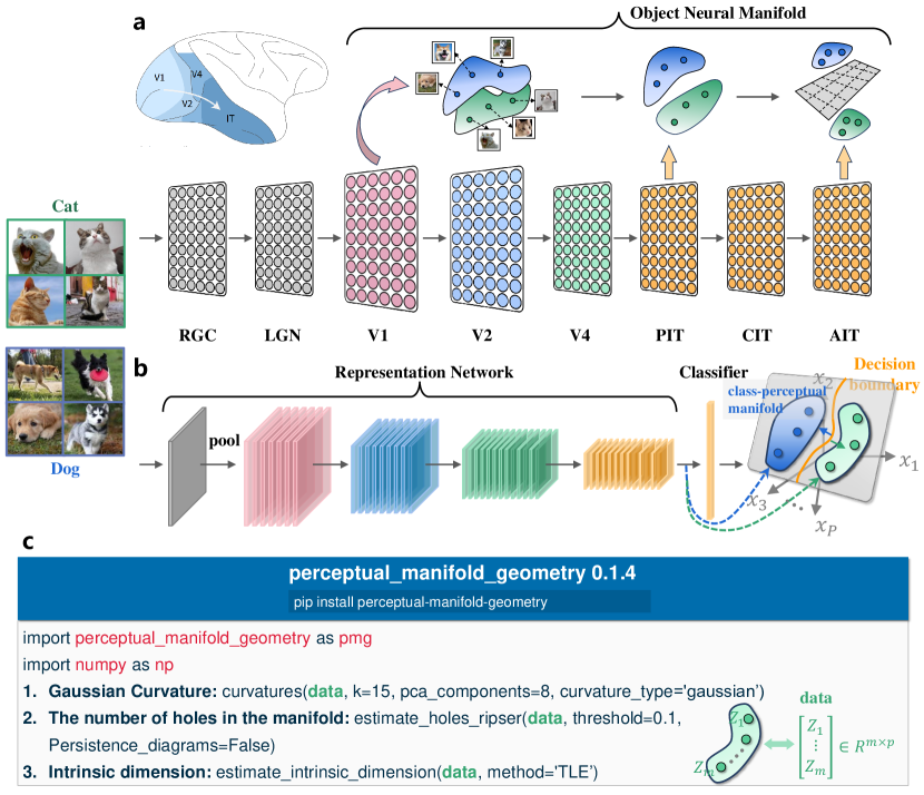
Figure 1: a, When stimulated by objects of the same category, the human visual system forms object manifolds. As the visual cortex progresses through its layers, the object manifolds of different objects become more distinguishable and flatter. b, Deep neural networks use representation networks to disentangle and reduce the dimensionality of data manifolds into class-specific perceptual manifolds, which are then used for object recognition by the classifier. c, Example calculations of Gaussian curvature, the number of topological holes, and intrinsic dimensionality for perceptual manifolds using the Perceptual-Manifold-Geometry toolkit.

Table 1: Summary of the experiments and results. LR denotes the learning rate and Mn denotes the momentum of the optimizer. If not specifically identified, the details of the experimental hyperparameters are shared in the Settings column. Green and red text denote the hyperparameters of the convolutional neural network and vision transformer, respectively.

Dataset	DNN	Settings
CIFAR-10	ViT-B/32, ViT-B/16	epoch: 200, 300
CIFAR-100	VGG-19	Optimizer: SGD
Mini-ImageNet	SeNet-50	Mm: 0.9
Caltech-101	ResNet-18, ResNet-34, ResNet-50	LR: 0.05, 0.001

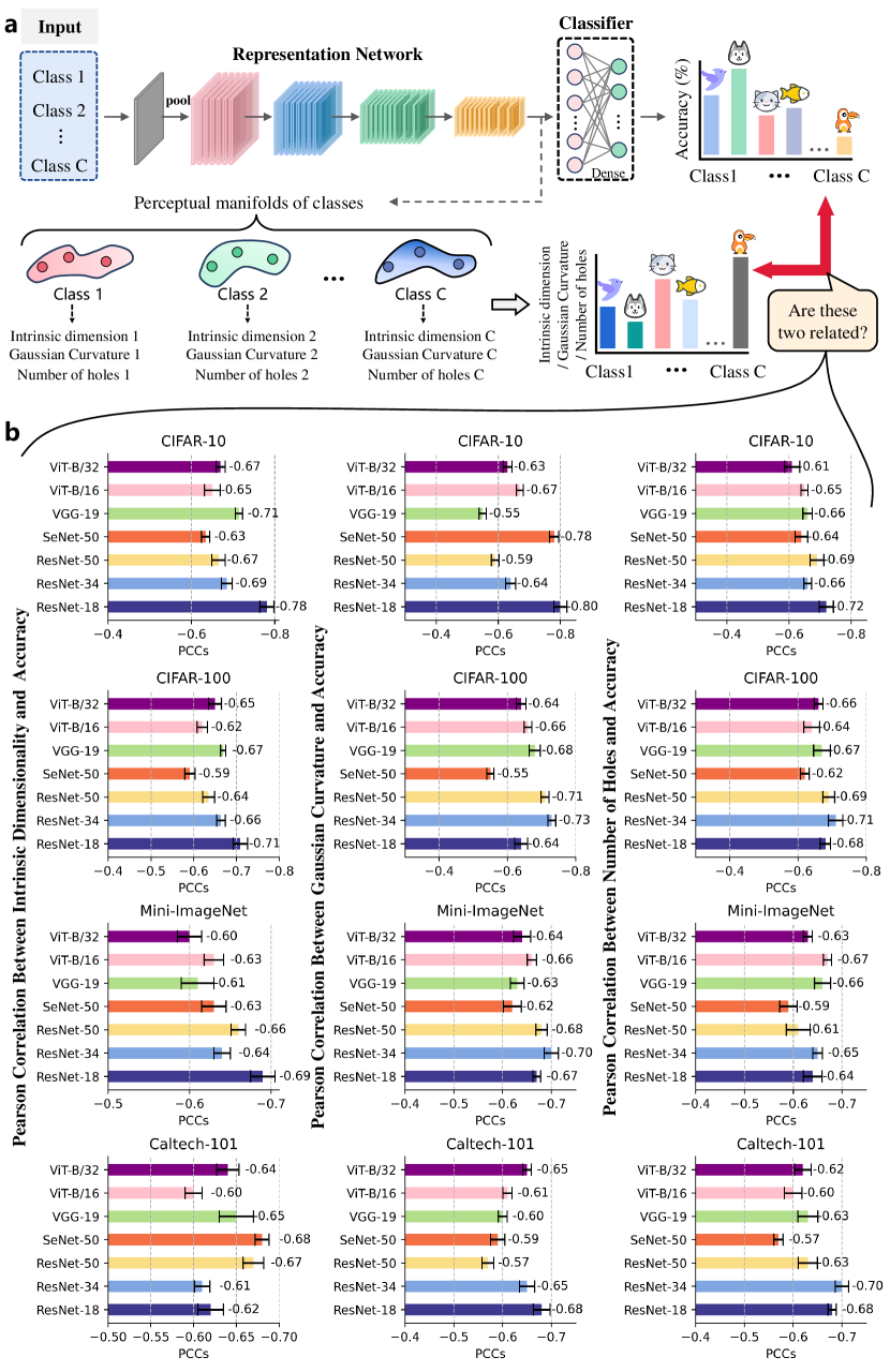
Figure 2: a, Using the representation network of a DNN to extract image embeddings for each class and calculating the geometric complexity of class-specific perceptual manifolds based on these embeddings. b, Bar charts showing Pearson correlation coefficients (PCCs) between class accuracy and various geometric complexities of class-specific perceptual manifolds across different datasets.

We first measured the recognition accuracy of fully trained DNNs on each class. As shown in Figure.2a, we then extracted the embeddings of images for each class from the representation network of the DNN and stored them separately. Subsequently, we estimated the geometric complexity of the perceptual manifolds corresponding to each class’s embeddings, including intrinsic dimensionality, Gaussian curvature, and the number of topological holes. We calculated the Pearson correlation coefficients between geometric complexity and class-wise recognition accuracy. As illustrated in Figure.2b, the experimental results on different datasets and DNN architectures reveal a significant negative correlation between the geometric complexity of class-specific perceptual manifolds and recognition accuracy. These findings confirm our hypothesis: differences in geometric complexity among class-specific perceptual manifolds contribute to inconsistent recognition performance across classes, thereby inducing bias. Furthermore, the higher the geometric complexity of a perceptual manifold, the more challenging it is for the model to recognize the corresponding class.

This finding can also be understood from the perspective of model optimization. Intrinsic dimensionality reflects the complexity of a manifold’s embedding. Higher dimensionality indicates more intricate manifold structures in high-dimensional space, requiring a classifier with greater capacity to effectively distinguish these samples. High Gaussian curvature typically signifies that the data distribution in the embedding space is more twisted and complex, leading to unstable decision boundaries and increasing classification difficulty. A higher number of topological holes implies more complex decision boundaries, making classifiers more prone to overfitting and resulting in poorer generalization performance. Our findings also offer new insights into mitigating model bias. By constraining optimization objectives, models can be encouraged to learn class-specific perceptual manifolds with lower and more balanced geometric complexity.

Inspired by human visual behavior, this study establishes a universal geometric analysis framework to explain the pervasive bias in DNNs—an achievement that was previously difficult to realize through algorithmic research alone. Experimental results demonstrate that DNNs not only structurally resemble the human visual system but also exhibit similar characteristics in their internal data compression and processing mechanisms. This discovery reinforces the confidence of researchers in brain-inspired artificial intelligence. As the Perceptual-Manifold-Geometry toolkit gains broader adoption, it is poised to provide valuable tools for artificial intelligence and neuroscience research. This work exemplifies the successful integration of neuroscience and computer science, highlighting the immense potential of interdisciplinary collaboration.

Methods

To facilitate the study of perceptual manifolds in DNNs, we developed the Perceptual-Manifold-Geometry toolkit, which provides a comprehensive framework for analyzing the geometric characteristics of class-specific perceptual manifolds. The toolkit includes modules for intrinsic dimensionality estimation, Gaussian curvature calculation, and topological quantification, focusing particularly on the number of topological holes. These features enable systematic analysis of the relationships between manifold geometry and recognition performance.

Estimation of the Intrinsic Dimension

Given a set of embeddings $Z=[z_{1},\dots,z_{n}]\in\mathbb{R}^{p\times n}$ corresponding to an image dataset, $Z$ is typically distributed near a low-dimensional perceptual manifold $M$ embedded in the $p$-dimensional space, akin to a two-dimensional plane in three-dimensional space. The intrinsic dimension $ID(M)$ of the perceptual manifold is such that $d<p$. A higher intrinsic dimension indicates a more complex perceptual manifold. The following describes how to use TLE to estimate the intrinsic dimension of the perceptual manifold formed by $Z=[z_{1},\dots,z_{n}]\in\mathbb{R}^{p\times n}$.

The primary method for estimating intrinsic dimension involves analyzing the distribution of distances between each point in the dataset and its neighboring points, and then estimating the dimensionality of the local space based on the rate of growth of distances or other statistic. Assuming that the distribution of samples is uniform within a small neighborhood, and then uses a Poisson process to simulate the number of points discovered by random sampling within neighborhoods of a given radius around each sample Levina and Bickel (2004). Subsequently, by constructing a likelihood function, the rate of growth in quantity is associated with the surface area of a sphere. Given any embedding $z_{i}$ in the dataset and its set of $k$ nearest neighbors $V$, the Maximum Likelihood Estimator (MLE) of the local intrinsic dimensiona at $z_{i}$ is given by:

$$ID_{MLE}(z_{i})=-\Bigg{(}\frac{1}{k}\sum_{j=1}^{k}ln\frac{r_{j}(z_{i})}{r_{k}(z_{i})}\Bigg{)}^{-1},$$

where $r_{j}(z_{i})$ represents the distance between $z_{i}$ and its $j$-th nearest neighbor. TLE Amsaleg et al. (2019) no longer assumes uniformity of sample distribution in local neighborhoods, thus closer to the true data distribution. It assumes the local intrinsic dimension to be continuous, thereby utilizing nearby sample points to stabilize estimates at $z_{i}$. Specifically, the estimate of the intrinsic dimension at $z_{i}$ using TLE is given by

$$ID_{TLE}(z_{i})=-\Bigg{(}\frac{1}{\left|V_{*}\right|^{2}}\sum_{\begin{subarray}{c}v,w\in V_{*}\\ v\neq w\end{subarray}}\Bigg{[}\ln\frac{d_{z_{i}}(v,w)}{r_{k}(z_{i})}+\ln\frac{d_{z_{i}}(2z_{i}-v,w)}{r_{k}(z_{i})}\Bigg{]}\Bigg{)}^{-1},$$ (1)

where $V_{*}=V\cup\{z_{i}\}$, and $d_{z_{i}}(v,w)$ is defined as $(r_{k}(z_{i})(w-v)\cdot(w-v))/(2(z_{i}-v)\cdot(w-v))$. Furthermore, the global intrinsic dimensionality of the perceptual manifold is estimated as the average of local intrinsic dimensionalities:

$$ID_{TLE}(Z)=\frac{1}{n}\sum_{i=1}^{n}ID_{TLE}(z_{i}).$$

Estimation of the Gaussian curvature

Given a point cloud perceptual manifold $M$, which consists of a $p$-dimensional point set $Z=[z_{1},\dots,z_{n}]\in\mathbb{R}^{p\times n}$, our goal is to calculate the Gauss curvature at each point. First, the normal vector at each point on $M$ is estimated by the neighbor points. Denote by $z_{i}^{j}$ the $j$-th neighbor point of $z_{i}$ and $u_{i}$ the normal vector at $z_{i}$. We solve for the normal vector by minimizing the inner product of $z_{i}^{j}-c_{i},j=1,\dots,k$ and $u_{i}$ Asao and Ike (2021), i.e.,

$$\min{\textstyle\sum_{j=1}^{k}}((z_{i}^{j}-c_{i})^{T}u_{i})^{2},$$

where $c_{i}=\frac{1}{k}{\textstyle\sum_{j=1}^{k}}z_{i}^{j}$ and $k$ is the number of neighbor points. Let $y_{j}=z_{i}^{j}-c_{i}$, then the optimization objective is converted to

$$\min{\textstyle\sum_{j=1}^{k}}(y_{j}^{T}u_{i})^{2}=\min{\textstyle\sum_{j=1}^{k}}u_{i}^{T}y_{j}y_{j}^{T}u_{i}=\min(u_{i}^{T}({\textstyle\sum_{j=1}^{k}}y_{j}y_{j}^{T})u_{i}).$$

${\textstyle\sum_{j=1}^{k}}y_{j}y_{j}^{T}$ is the covariance matrix of $k$ neighbors of $z_{i}$. Therefore, let $Y=[y_{1},\dots,y_{k}]\in\mathbb{R}^{p\times k}$ and ${\textstyle\sum_{j=1}^{k}}y_{j}y_{j}^{T}=YY^{T}$. The optimization objective is further equated to

$$\begin{cases}f(u_{i})=u_{i}^{T}YY^{T}u_{i},YY^{T}\in\mathbb{R}^{p\times p},\\ min(f(u_{i})),\\ s.t.u_{i}^{T}u_{i}=1.\end{cases}$$

Construct the Lagrangian function $L(u_{i},\lambda)=f(u_{i})-\lambda(u_{i}^{T}u_{i}-1)$ for the above optimization objective, where $\lambda$ is a parameter. The first-order partial derivatives of $L(u_{i},\lambda)$ with respect to $u_{i}$ and $\lambda$ are

$$\frac{\partial L(u_{i},\lambda)}{\partial u_{i}}=\frac{\partial}{\partial u_{i}}f(u_{i})-\lambda\frac{\partial}{\partial u_{i}}(u_{i}^{T}u_{i}-1)=2(YY^{T}u_{i}-\lambda u_{i}),$$

$$\frac{\partial L(u_{i},\lambda)}{\partial\lambda}=u_{i}^{T}u_{i}-1.$$

Let $\frac{\partial L(u_{i},\lambda)}{\partial u_{i}}$ and $\frac{\partial L(u_{i},\lambda)}{\partial\lambda}$ be $0$, we can get $YY^{T}u_{i}=\lambda u_{i},u_{i}^{T}u_{i}=1$. It is obvious that solving for $u_{i}$ is equivalent to calculating the eigenvectors of the covariance matrix $YY^{T}$, but the eigenvectors are not unique. From $\left\langle YY^{T}u_{i},u_{i}\right\rangle=\left\langle\lambda u_{i},u_{i}\right\rangle$ we can get $\lambda=\left\langle YY^{T}u_{i},u_{i}\right\rangle=u_{i}^{T}YY^{T}u_{i}$, so the optimization problem is equated to $\mathop{\arg\min}_{u_{i}}(\lambda)$. Performing the eigenvalue decomposition on the matrix $YY^{T}$ yields $p$ eigenvalues $\lambda_{1},\dots,\lambda_{p}$ and the corresponding $p$-dimensional eigenvectors $[\xi_{1},\dots,\xi_{p}]\in\mathbb{R}^{p\times p}$, where $\lambda_{1}\geq\dots\geq\lambda_{p}\geq 0$, $\left\|\xi_{i}\right\|_{2}=1,i=1,\dots,p$, $\left\langle\xi_{a},\xi_{b}\right\rangle=0(a\neq b)$. The eigenvector $\xi_{m+1}$ corresponding to the smallest non-zero eigenvalue of the matrix $YY^{T}$ is taken as the normal vector $u_{i}$ of $M$ at $z_{i}$.

Consider an $m$-dimensional affine space with center $z_{i}$, which is spanned by $\xi_{1},\dots,\xi_{m}$. This affine space approximates the tangent space at $z_{i}$ on $M$. We estimate the curvature of $M$ at $z_{i}$ by fitting a quadratic hypersurface in the tangent space utilizing the neighbor points of $z_{i}$. The $k$ neighbors of $z_{i}$ are projected into the affine space $z_{i}+\left\langle\xi_{1},\dots,\xi_{m}\right\rangle$ and denoted as

$$o_{j}=[(z_{i}^{j}-z_{i})\cdot\xi_{1},\dots,(z_{i}^{j}-z_{i})\cdot\xi_{m}]^{T}\in\mathbb{R}^{m},j=1,\dots,k.$$

Denote by $o_{j}[m]$ the $m$-th component $(z_{i}^{j}-z_{i})\cdot\xi_{m}$ of $o_{j}$. We use $z_{i}$ and $k$ neighbor points to fit a quadratic hypersurface $f(\theta)$ with parameter $\theta\in\mathbb{R}^{m\times m}$. The hypersurface equation is denoted as

$$f(o_{j},\theta)=\frac{1}{2}{\textstyle\sum_{a,b}}\theta_{a,b}o_{j}\left[a\right]o_{j}\left[b\right],j\in\left\{1,\dots,k\right\},$$

further, minimize the squared error

$$E(\theta)={\textstyle\sum_{j=1}^{k}}(\frac{1}{2}{\textstyle\sum_{a,b}}\theta_{a,b}o_{j}\left[a\right]o_{j}\left[b\right]-(z_{i}^{j}-z_{i})\cdot u_{i})^{2}.$$

Let $\frac{\partial E(\theta)}{\partial\theta_{a,b}}=0,a,b\in\left\{1,\dots,m\right\}$ yield a nonlinear system of equations, but it needs to be solved iteratively. Here, we propose an ingenious method to fit the hypersurface and give the analytic solution of the parameter $\theta$ directly. Expand the parameter $\theta$ of the hypersurface into the column vector

$$\theta=\left[\theta_{1,1},\dots,\theta_{1,m},\theta_{2,1},\dots,\theta_{m,m}\right]^{T}\in\mathbb{R}^{m^{2}}.$$

Organize the $k$ neighbor points $\left\{o_{j}\right\}_{j=1}^{k}$ of $z_{i}$ according to the following form:

$$O(z_{i})=\begin{bmatrix}o_{1}\left[1\right]o_{1}\left[1\right]&o_{1}\left[1\right]o_{1}\left[2\right]&\cdots&o_{1}\left[m\right]o_{1}\left[m\right]\\ o_{2}\left[1\right]o_{2}\left[1\right]&o_{2}\left[1\right]o_{2}\left[2\right]&\cdots&o_{2}\left[m\right]o_{2}\left[m\right]\\ \vdots&\vdots&\ddots&\vdots\\ o_{k}\left[1\right]o_{k}\left[1\right]&o_{k}\left[1\right]o_{k}\left[2\right]&\cdots&o_{k}\left[m\right]o_{k}\left[m\right]\end{bmatrix}\in\mathbb{R}^{k\times m^{2}}.$$

The target value is

$$T=\left[(z_{i}^{1}-z_{i})\cdot u_{i},(z_{i}^{2}-z_{i})\cdot u_{i},\dots,(z_{i}^{k}-z_{i})\cdot u_{i}\right]^{T}\in\mathbb{R}^{k}.$$

We minimize the squared error

$$E(\theta)=\frac{1}{2}tr\left[\left(O(z_{i})\theta-T\right)^{T}(O(z_{i})\theta-T)\right],$$

and find the partial derivative of $E(\theta)$ for $\theta$:

$$\frac{\partial E(\theta)}{\partial\theta}=\frac{1}{2}\left(\frac{\partial tr(\theta^{T}O(z_{i})^{T}O(z_{i})\theta)}{\partial\theta}-\frac{\partial tr(\theta^{T}O(z_{i})^{T}T)}{\partial\theta}\right)$$

$$=O(z_{i})^{T}O(z_{i})\theta-O(z_{i})^{T}T.$$

Let $\frac{\partial E(\theta)}{\partial\theta}=0$, we can get

$$\theta=(O(z_{i})^{T}O(z_{i}))^{-1}O(z_{i})^{T}T.$$

Thus, the Gauss curvature of the perceptual manifold $M$ at $z_{i}$ can be calculated as

$$G(z_{i})=det(\theta)=det((O(z_{i})^{T}O(z_{i}))^{-1}O(z_{i})^{T}T).$$

Up to this point, we provide an approximate solution of the Gauss curvature at any point on the point cloud perceptual manifold $M$. Recent research Balestriero, Pesenti, and LeCun (2021) shows that on a high-dimensional dataset, almost all samples lie on convex locations, and thus the complexity of the perceptual manifold is defined as the average $\frac{1}{n}{\textstyle\sum_{i=1}^{n}}G(z_{i})$ of the Gauss curvatures at all points on $M$. Our approach does not require iterative optimization and can be quickly deployed in a deep neural network to calculate the Gauss curvature of the perceptual manifold.

Estimation of the Number of Holes

To analyze the geometric complexity of perceptual manifolds, this study employs Persistent Homology, a technique from Topological Data Analysis (TDA), to quantify the topological hole features in data manifolds. This method reveals topological properties, such as connectivity, loops, and void distributions in high-dimensional data embeddings, offering a geometric perspective for understanding the feature spaces learned by Deep Neural Networks (DNNs) Carlsson (2009).

Specifically, given a dataset $X\subset\mathbb{R}^{d}$, the Ripser algorithm is used to compute its Persistence Diagram, capturing the evolution of topological structures at different scales. The persistence diagram represents the topological complexity of the manifold by recording the birth and death times of each topological feature. In this study, we focus on 1-dimensional homology $H_{1}$, which corresponds to loop structures, where the total number of loops reflects the number of holes in the data manifold.

To enhance computational robustness, a persistence threshold $\tau$ is introduced to filter out low-persistence features caused by noise. Let $\text{Persistence}=\text{Death}-\text{Birth}$; only loops with $\text{Persistence}>\tau$ are retained as significant features. The number of holes is then defined as the total count of these significant loops. Additionally, to characterize the spatial distribution of holes comprehensively, we compute their total persistence, average persistence, and persistence density (defined as the ratio of total persistence to the time span of features). This method, implemented efficiently using tools such as Ripser Bauer (2021), extracts key topological attributes of the data without significantly increasing computational complexity. These topological metrics not only reveal the geometric complexity of perceptual manifolds but also provide a theoretical foundation for understanding their influence on classifier decision boundaries.

Conflict of Interest Statement

The author (authors) has (have) no conflicts to disclose.

Author contributions

Yanbiao Ma: Conceptualization, Data curation, Formal analysis, Investigation, Methodology, Software, Writing – original draft. Bowei Liu: Conceptualization, Data curation, Formal analysis, Investigation, Methodology, Software. Wei Dai: Conceptualization, Data curation, Formal analysis, Investigation, Methodology, Software. Jiayi Chen: Resources, Writing – review & editing. Shuo Li: Funding acquisition, Validation. All authors have read and agreed to the published version of the manuscript.

Data availability

All deep neural networks used in this study have been appropriately cited in the main text. All datasets utilized in this research are open access and have been referenced in the paper. The web links to the datasets are as follows: CIFAR-10/100 (https://www.cs.toronto.edu/˜kriz/cifar.html), Caltech-101 (https://www.vision.caltech.edu/datasets/). The Mini-ImageNet dataset is derived from ImageNet and can be generated using the MLclf package (https://github.com/tiger2017/MLclf). Additionally, the toolkit developed for calculating the geometric properties of perceptual manifolds has been officially released and is available at https://github.com/mayanbiao1234/Geometric-metrics-for-perceptual-manifolds.

References

- Chiu et al. (2024) I.-M. Chiu, T.-Y. Huang, D. Ouyang, W.-C. Lin, Y.-J. Pan, C.-Y. Lu, and K.-H. Kuo, “Pact-3d, a deep learning algorithm for pneumoperitoneum detection in abdominal ct scans,” Nature Communications 15, 9660 (2024).
- Li et al. (2022) J. Li, S. Chen, X. Pan, Y. Yuan, and H.-B. Shen, “Cell clustering for spatial transcriptomics data with graph neural networks,” Nature Computational Science 2, 399–408 (2022).
- Jiang et al. (2022) S. Jiang, Y. Zhu, C. Liu, X. Song, X. Li, and W. Min, “Dataset bias in few-shot image recognition,” IEEE Transactions on Pattern Analysis and Machine Intelligence 45, 229–246 (2022).
- Hu et al. (2024) T. Hu, Y. Kyrychenko, S. Rathje, N. Collier, S. van der Linden, and J. Roozenbeek, “Generative language models exhibit social identity biases,” Nature Computational Science , 1–11 (2024).
- Yang et al. (2022) L. Yang, H. Jiang, Q. Song, and J. Guo, “A survey on long-tailed visual recognition,” International Journal of Computer Vision 130, 1837–1872 (2022).
- Alshammari et al. (2022) S. Alshammari, Y.-X. Wang, D. Ramanan, and S. Kong, “Long-tailed recognition via weight balancing,” in Proceedings of the IEEE/CVF conference on computer vision and pattern recognition (2022) pp. 6897–6907.
- Ma et al. (2023a) Y. Ma, L. Jiao, F. Liu, Y. Li, S. Yang, and X. Liu, “Delving into semantic scale imbalance,” in The Eleventh International Conference on Learning Representations (2023).
- Kaushik et al. (2024) C. Kaushik, R. Liu, C.-H. Lin, A. Khera, M. Y. Jin, W. Ma, V. Muthukumar, and E. L. Dyer, “Balanced data, imbalanced spectra: Unveiling class disparities with spectral imbalance,” arXiv preprint arXiv:2402.11742 (2024).
- Langdon, Genkin, and Engel (2023) C. Langdon, M. Genkin, and T. A. Engel, “A unifying perspective on neural manifolds and circuits for cognition,” Nature Reviews Neuroscience 24, 363–377 (2023).
- DiCarlo and Cox (2007) J. J. DiCarlo and D. D. Cox, “Untangling invariant object recognition,” Trends in cognitive sciences 11, 333–341 (2007).
- Peelen, Berlot, and de Lange (2024) M. V. Peelen, E. Berlot, and F. P. de Lange, “Predictive processing of scenes and objects,” Nature Reviews Psychology 3, 13–26 (2024).
- Li and Wang (2023) X. Li and S. Wang, “Toward a computational theory of manifold untangling: from global embedding to local flattening,” Frontiers in Computational Neuroscience 17, 1197031 (2023).
- Chong and Feng (2024) N. J. L. Chong and L. Feng, “Self-organization toward 1/f noise in deep neural networks,” Chaos: An Interdisciplinary Journal of Nonlinear Science 34 (2024).
- Krizhevsky, Sutskever, and Hinton (2012) A. Krizhevsky, I. Sutskever, and G. E. Hinton, “Imagenet classification with deep convolutional neural networks,” Advances in neural information processing systems 25 (2012).
- Bollt (2024) E. Bollt, “How neural networks work: Unraveling the mystery of randomized neural networks for functions and chaotic dynamical systems,” Chaos: An Interdisciplinary Journal of Nonlinear Science 34 (2024).
- Ma et al. (2023b) Y. Ma, L. Jiao, F. Liu, S. Yang, X. Liu, and L. Li, “Curvature-balanced feature manifold learning for long-tailed classification,” in Proceedings of the IEEE/CVF conference on computer vision and pattern recognition (2023) pp. 15824–15835.
- Cohen et al. (2020) U. Cohen, S. Chung, D. D. Lee, and H. Sompolinsky, “Separability and geometry of object manifolds in deep neural networks,” Nature communications 11, 746 (2020).
- Greco and Siegel (2024) A. Greco and M. Siegel, “A spatiotemporal style transfer algorithm for dynamic visual stimulus generation,” Nature Computational Science , 1–15 (2024).
- Krizhevsky and Hinton (2009) A. Krizhevsky and G. Hinton, “Learning multiple layers of features from tiny images,” Master’s thesis, Department of Computer Science, University of Toronto (2009).
- Deng et al. (2009) J. Deng, W. Dong, R. Socher, L.-J. Li, K. Li, and L. Fei-Fei, “Imagenet: A large-scale hierarchical image database,” in 2009 IEEE conference on computer vision and pattern recognition (Ieee, 2009) pp. 248–255.
- Fei-Fei, Fergus, and Perona (2007) L. Fei-Fei, R. Fergus, and P. Perona, “Learning generative visual models from few training examples: An incremental bayesian approach tested on 101 object categories,” Computer vision and Image understanding 106, 59–70 (2007).
- He et al. (2016) K. He, X. Zhang, S. Ren, and J. Sun, “Deep residual learning for image recognition,” in Proceedings of the IEEE conference on computer vision and pattern recognition (2016) pp. 770–778.
- Dosovitskiy (2020) A. Dosovitskiy, “An image is worth 16x16 words: Transformers for image recognition at scale,” arXiv preprint arXiv:2010.11929 (2020).
- Levina and Bickel (2004) E. Levina and P. Bickel, “Maximum likelihood estimation of intrinsic dimension,” Advances in neural information processing systems 17 (2004).
- Amsaleg et al. (2019) L. Amsaleg, O. Chelly, M. E. Houle, K.-i. Kawarabayashi, M. Radovanović, and W. Treeratanajaru, “Intrinsic dimensionality estimation within tight localities,” in Proceedings of the 2019 SIAM international conference on data mining (SIAM, 2019) pp. 181–189.
- Asao and Ike (2021) Y. Asao and Y. Ike, “Curvature of point clouds through principal component analysis,” arXiv preprint arXiv:2106.09972 (2021).
- Balestriero, Pesenti, and LeCun (2021) R. Balestriero, J. Pesenti, and Y. LeCun, “Learning in high dimension always amounts to extrapolation,” arXiv preprint arXiv:2110.09485 (2021).
- Carlsson (2009) G. Carlsson, “Topology and data,” Bulletin of the American Mathematical Society 46, 255–308 (2009).
- Bauer (2021) U. Bauer, “Ripser: efficient computation of vietoris–rips persistence barcodes,” Journal of Applied and Computational Topology 5, 391–423 (2021).