Empirical plunge profiles of
time-frequency localization operators

Abstract.

For time-frequency localization operators with symbol $R\Omega$, we work out the exact large $R$ eigenvalue behavior for rotationally invariant $\Omega$ and conjecture that the same relation holds for all scaled symbols $R\Omega$ as long as the window is the standard Gaussian. Specifically, we conjecture that the $k$-th eigenvalue of the localization operator with symbol $R\Omega$ converges to $\frac{1}{2}\operatorname{erfc}\big{(}\sqrt{2\pi}\frac{k-|R\Omega|}{|\partial R\Omega|}\big{)}$ as $R\to\infty$. To support the conjecture, we compute the eigenvalues of discrete frame multipliers with various symbols using LTFAT and find that they agree with the behavior of the conjecture to a large degree.

1. Introduction and background

When restricting a signal $f\in L^{2}(\mathbb{R}^{d})$ to a subset of the time-frequency plane, there are two main approaches. The simpler is to consider a spatial cutoff, followed by a Fourier multiplier, followed by the same spatial cutoff once more. For sets $E,F\subset\mathbb{R}^{2d}$ and $\mathcal{F}$ the Fourier transform, we can write such operators as

(1) $$Sf=\chi_{F}\mathcal{F}^{-1}\chi_{E}\mathcal{F}\chi_{F}f$$

where $\chi_{\Omega}$ is the indicator function of the set $\Omega$. While such an operator does not yield a function compactly supported in both time and frequency, as that is prohibited by the uncertainty principle, it approximately does so provided $E,F$ are large enough. This line of work goes back to Landau, Pollak and Slepian, starting in the 1960s [25, 17, 18, 26, 24], who showed many of the classical properties of these operators which we will refer to as Fourier concentration operators following [21].

Another more general way to restrict a signal to a subset $\Omega\subset\mathbb{R}^{2d}$ of the time-frequency plane is to apply the multiplication operator on a time-frequency representation of $f$. Specifically, using the short-time Fourier transform (STFT) [12], defined with a window function $g\in L^{2}(\mathbb{R}^{d})$ as

$$V_{g}f(x,\omega)=\int_{\mathbb{R}^{d}}f(t)\overline{g(t-x)}e^{-2\pi i\omega t}\,dt=\langle f,\pi(x,\omega)g\rangle,$$

where $\pi(x,\omega)f(t)=M_{\omega}T_{x}f(t)=e^{2\pi i\omega\cdot t}f(t-x)$ is a time-frequency shift, we can define the localization operator $A_{\Omega}^{g}$ as

$$A_{\Omega}^{g}f=\int_{\Omega}V_{g}f(x,\omega)\pi(x,\omega)g\,dx\,d\omega.$$

If $\Omega=\mathbb{R}^{2d}$, this is just the identity operator on $L^{2}(\mathbb{R}^{d})$, provided $g$ is normalized, but for a compact $\Omega$ we get a compact self-adjoint operator. Localization operators were first considered in the time-frequency context by Daubechies [5].

In both cases, the operators can be interpreted as projection operators onto either the subspace $F\times E$ or $\Omega$ of the time-frequency plane. The number of orthogonal functions which fit in these subspaces is approximately equal to the area of the subset of the time-frequency plane and consequently the corresponding eigenvalues are close to $1$. This is followed by what is commonly referred to as the plunge region where the eigenvalues rapidly decay to $0$. All eigenvalues in the plunge region $\delta<\lambda_{k}<1-\delta$ correspond to eigenfunctions which are partially supported inside and outside the subset $\Omega$ of the time-frequency plane. As these eigenfunctions are orthogonal, they each occupy a part of $\partial\Omega$ and we therefore expect the number of eigenvalues in the plunge region to depend on the size of $\partial\Omega$.

1.1. Earlier results

For Fourier concentration operators, these intuitions have been quantified with quite some success. The number of eigenvalues close to one was shown to be approximately equal to $|E|\cdot|F|$ for $E,F$ intervals by Landau in [16]. In particular, for any $\delta>0$, the quantity

(2) $$\frac{\#\{k:\lambda_{k}>1-\delta\}}{|E|\cdot|F|}$$

approaches $1$ as we dilate $E$ and $F$. The size of the plunge region, meaning the number of eigenvalues between $\delta$ and $1-\delta$, was also bounded by $\log(|E|\cdot|F|)$ up to a constant.

In the more general setting of compact $E$ and $F$, Marceca, Romero and Speckbacher [21] showed under mild conditions that the size of the plunge region is bounded by

$$\frac{|\partial E|}{\kappa_{\partial E}}\frac{|\partial F|}{\kappa_{\partial F}}\log\left(\frac{|\partial E||\partial F|}{\kappa_{\partial E}\delta}\right)^{2d(1+\alpha)+1}$$

up to a constant factor, where $\kappa_{\partial E}$ is the maximal Ahlfors regular boundary constant of $E$, $\alpha$ is some number in $(0,1/2)$ and $|\partial E|$ is the $(d-1)$-dimensional Hausdorff measure of the boundary $\partial E$.

There are also more detailed asymptotics on the eigenvalue behavior near the plunge region, see [15] and references therein for an overview of these results.

Less is known in the case of time-frequency localization operators and this is what we aim to start to address in this paper. The number of eigenvalues close to $1$ was first bounded by Ramanathan and Topiwala in [23] by showing that

(3) $$\frac{\#\{k:\lambda_{k}^{\Omega}>1-\delta\}}{|\Omega|}$$

also converges to $1$ as $\Omega$ is dilated. As a byproduct of the proof, one also finds the upper limit

$$\big{|}\#\{k:\lambda_{k}^{\Omega}>1-\delta\}-|\Omega|\big{|}\leq C|\partial\Omega|$$

but no equivalence. Similar results are also available for Gabor multipliers, the discrete variant of localization operators, see e.g. [8, 9].

1.2. Our contribution

We will show that in the case of a rotationally invariant symbol, meaning a disk, annuli or union of annuli, the eigenvalues of localization operators can be computed explicitly and asymptotically exhibit an $\operatorname{erfc}$ (complementary error function) decay after $|\Omega|$ eigenvalues, over a range proportional to $|\partial\Omega|$. We conjecture that this behavior is universal for all symbols $\Omega$ as long as the window is the standard Gaussian and support the conjecture by verifying it numerically for a diverse collection of $\Omega$ with small error.

2. Eigenvalue behavior

2.1. Eigenvalues on disks, annuli, and rotationally invariant sets

In the original article on time-frequency localization operators [5], a general formula for computing the eigenvalues of localization operators with Gaussian window $g_{0}(t)=2^{1/4}e^{-\pi t^{2}}$ and a rotationally invariant symbol was given. Specialized to the case $\Omega=B(0,R),d=1$ and with our normalization conventions, we get

(4) $$\lambda_{k}^{B(0,R)}=1-e^{-\pi R^{2}}\sum_{j=0}^{k}\frac{(\pi R^{2})^{j}}{j!}.$$

from [5, Eq. (19c)]. Through a connection with the Poisson distribution, the large $R$ asymptotics of this can be computed neatly.

Theorem 2.1.

Let $\lambda_{k}^{R}$ be the $k$-th eigenvalue of the localization operator with symbol $B(0,R)$. It then holds that

(5) $$\left|\lambda_{k}^{R}-\frac{1}{2}\operatorname{erfc}\left(\frac{k-\pi R^{2}}{\sqrt{2\pi}R}\right)\right|=O\left(\frac{1}{R}\right)$$

where $\operatorname{erfc}$ is the complementary error function.

Proof.

We recognize (4) as the Poisson cumulative distribution function (CDF) with parameter $\pi R^{2}$. Specifically, if $X\sim\operatorname{Po}(\pi R^{2})$, then

$$\lambda_{k}^{R}=1-\mathbb{P}(X\leq k).$$

For large $R$, the Poisson distribution $\operatorname{Po}(\pi R^{2})$ can be approximated by a normal distribution with mean and variance $\pi R^{2}$ due to the central limit theorem. Therefore, we can approximate the CDF of $X$ as

$$\mathbb{P}(X\leq k)\approx\Phi\left(\frac{k-\pi R^{2}}{\sqrt{\pi R^{2}}}\right),$$

where $\Phi$ is the standard normal CDF.

Substituting this approximation into our expression for $\lambda_{k}^{R}$, we obtain

$$\lambda_{k}^{R}\approx 1-\Phi\left(\frac{k-\pi R^{2}}{\sqrt{\pi R^{2}}}\right).$$

Now recall that the complementary error function is related to the standard normal $\Phi$ by

$$\Phi(z)=\frac{1}{2}\left[1+\operatorname{erf}\left(\frac{z}{\sqrt{2}}\right)\right]\implies 1-\Phi(z)=\frac{1}{2}\operatorname{erfc}\left(\frac{z}{\sqrt{2}}\right).$$

Applying this to our expression for $\lambda_{k}^{R}$, we find that

$$\lambda_{k}^{R}\approx\frac{1}{2}\operatorname{erfc}\left(\frac{k-\pi R^{2}}{\sqrt{2\pi}R}\right).$$

To quantify the error in this approximation, we employ the Berry-Esseen theorem, which provides a bound on the difference between the Poisson CDF and its normal approximation. For the Poisson distribution, the Berry-Esseen bound states that

$$\left|\mathbb{P}(X\leq k)-\Phi\left(\frac{k-\pi R^{2}}{\sqrt{\pi R^{2}}}\right)\right|=O\left(\frac{1}{\sqrt{\pi R^{2}}}\right)=O\left(\frac{1}{R}\right).$$

Consequently, the difference between $\lambda_{k}^{R}$ and its normal approximation satisfies

$$\left|\lambda_{k}^{R}-\frac{1}{2}\operatorname{erfc}\left(\frac{k-\pi R^{2}}{\sqrt{2\pi}R}\right)\right|=O\left(\frac{1}{R}\right)$$

which is what we wished to show. ∎

Remark.

In [5] the large $R$ eigenvalue behavior is only investigated for fixed $k$ which just tells us how quickly $\lambda_{k}^{R}\to 1$ as $R\to\infty$, not the full $\operatorname{erfc}$ behavior. Still, the eigenvalue formula (4) and the rest of the results of [5] are so well known that Theorem 2.1 should perhaps be considered folklore in the field. Still, we have found no reference for it in the literature and so we include a proof in the interest of completion while making no claim of originality.

Remark.

The corresponding eigenvalue formula for $d>1$ is also available in [5] but is dependent on a multiindex $k$. To make computations simpler, we have chosen to restrict ourselves to the $d=1$ case.

While the above theorem was specialized to the case of a disk centered at $0$, the same eigenvalue behavior can be observed irrespective of the center of the disk. To see this, recall that for disks centered at $0$ it is the Hermite functions $(h_{k})_{k}$ which are the eigenfunctions. Now using that

$$\langle A_{B(0,R)}^{g_{0}}h_{k},h_{k}\rangle=\lambda_{k},$$

we can see that $\pi(z_{0})h_{k}$ is an eigenfunction with the same eigenvalue for the localization operator $A_{B(z_{0},R)}^{g_{0}}$. Indeed, with the change of variables $w=z-z_{0}$,

$$\big{\langle}A_{B(z_{0},R)}^{g_{0}}(\pi(z_{0})h_{k}),\pi(z_{0})h_{k}\big{\rangle} =\int_{B(z_{0},R)}V_{g_{0}}(\pi(z_{0})h_{k})(z)\langle\pi(z)g_{0},\pi(z_{0})h_{k}\rangle\,dz$$

$$=\int_{B(0,R)}\langle\pi(z_{0})h_{k},\pi(z_{0}+w)g_{0}\rangle\langle\pi(z_{0}+w)g_{0},\pi(z_{0})h_{k}\rangle\,dz$$

$$=\int_{B(0,R)}\langle h_{k},\pi(w)g_{0}\rangle\langle\pi(w)g_{0},h_{k}\rangle\,dz=\lambda_{k}$$

where we in the second to last step canceled out two phase factors. This means that we have the same $\operatorname{erfc}$ eigenvalue decay no matter where the disk is centered.

In the case where $\Omega$ is an annulus, which we will take to be centered at $0$ in the interest of brevity, we also have an $\operatorname{erfc}$ eigenvalue decay but we will have to work a little harder to show it. For a deeper discussion on localization operators with annuli as symbols, see [2].

Proposition 2.2.

Let $\lambda_{k}^{R}$ be the $k$-th eigenvalue of the localization operator with symbol $B(0,R)\setminus B(0,rR)$ for $r<1$. It then holds that

(6) $$\left|\lambda_{k}^{R}-\frac{1}{2}\operatorname{erfc}\left(\frac{k-\pi R^{2}(1-r^{2})}{\sqrt{2\pi}R(1+r)}\right)\right|=O\left(\frac{1}{R}\right).$$

Proof.

In this situation, the eigenfunctions of $A_{B(0,R)\setminus B(0,rR)}^{g_{0}}$ are still the Hermite functions and the unordered eigenvalues can be written as

(7) $$\lambda_{k}^{B(0,R)\setminus B(0,rR)}=\lambda_{k}^{B(0,R)}-\lambda_{k}^{B(0,rR)}$$

where $\lambda_{k}^{B(0,R)}$ are the eigenvalues from Theorem 2.1. As $R\to\infty$, this quantity will converge to

(8) $$f(k)=\frac{1}{2}\left[\operatorname{erfc}\left(\frac{k-\pi R^{2}}{\sqrt{2\pi}R}\right)-\operatorname{erfc}\left(\frac{k-\pi(rR)^{2}}{\sqrt{2\pi}rR}\right)\right]$$

with error bounded by $O(1/R)$. However, (7) is not ordered decreasingly. Writing $\mu_{k}=\lambda_{k}^{B(0,R)}-\lambda_{k}^{B(0,rR)}$ and letting $\mu_{k}^{*}$ denote the $k$-th element of the ordered collection $(\mu_{k})_{k}$, then $\mu_{k}^{*}$ is the $k$-th eigenvalue $\lambda_{k}^{R}$. To relate this to $f$ we will let $f^{*}$ denote the decreasing rearrangement $f^{*}:\mathbb{R}^{+}\to\mathbb{R}$ of $f$ and show that

$$\mu_{k}=f(k)\implies|\mu_{k}^{*}-f^{*}(k)|\leq\|f^{\prime}\|_{\infty}.$$

Let $\bar{f}$ be defined so that $\bar{f}(k)=\mu_{k}$ for integers $k$ and $\bar{f}$ is constant on all intervals $[k,k+1)$. Then

$$\big{|}\bar{f}(x)-f(x)\big{|}=\big{|}f(\lfloor x\rfloor)-f(x)\big{|}\leq\|f^{\prime}\|_{\infty}\big{|}x-\lfloor x\rfloor\big{|}\leq\|f^{\prime}\|_{\infty},$$

i.e., $\|\bar{f}-f\|_{\infty}<\|f^{\prime}\|_{\infty}$. Meanwhile $\mu_{k}^{*}=\bar{f}^{*}(k)$ so

$$\big{|}\mu_{k}^{*}-f^{*}(k)\big{|}=\big{|}\bar{f}^{*}(k)-f^{*}(k)\big{|}\leq\big{\|}\bar{f}^{*}-f^{*}\big{\|}_{\infty}\leq\big{\|}\bar{f}-f\big{\|}_{\infty}$$

by $\|g^{*}-h^{*}\|_{\infty}\leq\|g-h\|_{\infty}$ for general functions $g,h$, see [19, Chapter 3] for a proof. It is easy to see that $\|f^{\prime}\|_{\infty}=O(1/R)$ so we can conclude that

(9) $$|\lambda_{k}-f^{*}(k)|=O\left(\frac{1}{R}\right).$$

To construct the rearrangement $f^{*}$, we will let two cursors traverse the two $\operatorname{erfc}$ functions at the same height but different locations along the $x$-axis. Specifically, let

$$x_{1}(t)=t\sqrt{2\pi}R+\pi R^{2},\qquad x_{2}(t)=-t\sqrt{2\pi}rR+\pi(rR)^{2}.$$

These two cursors meet at $t=t_{0}=\frac{-\pi R^{2}(1-r)}{\sqrt{2\pi}R}$ however this is not necessarily the highest point of $f$. We would like to be able to traverse the two sides of $f$ at the same time at the same heights but this is not quite possible with our $x_{1},x_{2}$. Consider instead the alternative function $\tilde{f}$ which is defined as

$$\tilde{f}(x_{2}(t)):=f(x_{1}(t))$$

for $t\in[t_{0},\infty)$ and $\tilde{f}=f$ on $x_{1}([t_{0},\infty))$. This construction is well-defined because $x_{1}$ and $x_{2}$ perfectly divide up all of $\mathbb{R}$. We can now bound the error $|f-\tilde{f}|$ as

$$\big{\|}f -\tilde{f}\big{\|}_{\infty}=\sup_{t\geq t_{0}}|f(x_{1}(t))-f(x_{2}(t))|$$

$$=\frac{1}{2}\sup_{t\geq t_{0}}\left|2-\operatorname{erfc}\left(\frac{t\sqrt{2\pi}R+\pi R^{2}(1-r^{2})}{\sqrt{2\pi}rR}\right)-\operatorname{erfc}\left(\frac{-t\sqrt{2\pi}rR-\pi R^{2}(1-r^{2})}{\sqrt{2\pi}R}\right)\right|$$

where we used that $\operatorname{erfc}(t)+\operatorname{erfc}(-t)=2$. Since $\operatorname{erfc}$ is a decreasing function, we can bound this quantity using first that

$$\operatorname{erfc}\left(\frac{t\sqrt{2\pi}R+\pi R^{2}(1-r^{2})}{\sqrt{2\pi}rR}\right) \leq\operatorname{erfc}\left(\frac{t_{0}\sqrt{2\pi}R+\pi R^{2}(1-r^{2})}{\sqrt{2\pi}rR}\right)$$

(10) $$=\operatorname{erfc}\left(\frac{\pi R^{2}(r-r^{2})}{\sqrt{2\pi}rR}\right)=O\left(\frac{1}{R}\right)$$

where we used that $\operatorname{erfc}(z)=\frac{e^{-z^{2}}}{\sqrt{\pi}z}+O\big{(}\frac{1}{z^{2}}\big{)}$ [7, §7.12(i)]. Now $2-\operatorname{erfc}(x)$ is an increasing function so it can be bounded from above by plugging in $t=t_{0}$ since the argument is decreasing in $t$. This means that

$$2-\operatorname{erfc}\left(\frac{-t\sqrt{2\pi}rR-\pi R^{2}(1-r^{2})}{\sqrt{2\pi}R}\right) \leq 2-\operatorname{erfc}\left(\frac{-t_{0}\sqrt{2\pi}rR-\pi R^{2}(1-r^{2})}{\sqrt{2\pi}R}\right)$$

$$=2-\operatorname{erfc}\left(\frac{-\pi R^{2}(1-r)}{\sqrt{2\pi}R}\right)$$

$$=\operatorname{erfc}\left(\frac{\pi R^{2}(1-r)}{\sqrt{2\pi}R}\right)=O\left(\frac{1}{R}\right).$$

Having established $\|f-\tilde{f}\|_{\infty}$ is small, it also follows that the two rearrangements $f^{*}$ and $\tilde{f}^{*}$ satisfy

$$\big{\|}f^{*}-\tilde{f}^{*}\big{\|}_{\infty}\leq\big{\|}f-\tilde{f}\big{\|}_{\infty}$$

from [19, Chapter 3] again. It still remains to write out the rearrangement $\tilde{f}^{*}(x)$. To do so, we introduce another cursor $x(t)$ which should map $t_{0}$ to $0$. We also make the ansatz that $x(t)$ is linear in $t$, i.e., of the form $x(t)=at+b$. To preserve the total mass, for each $dt$ we should add the mass from $\tilde{f}(x_{1}(t))$ and $\tilde{f}(x_{2}(t))$ combined to $\tilde{f}^{*}(x(t))$. Using that $\tilde{f}(x_{2}(t))=\tilde{f}(x_{1}(t))=f(x_{1}(t))$, this means that

$$\tilde{f}^{*}(x(t))\frac{dx}{dt}dt =\tilde{f}(x_{1}(t))\left|\frac{dx_{1}}{dt}\right|dt+\tilde{f}(x_{2}(t))\left|\frac{dx_{2}}{dt}\right|dt$$

$$=f(x_{1}(t))\left(\left|\frac{dx_{1}}{dt}\right|+\left|\frac{dx_{2}}{dt}\right|\right)dt$$

$$=\frac{1}{2}\left[\operatorname{erfc}(t)-\operatorname{erfc}\left(\frac{t\sqrt{2\pi}R+\pi R^{2}(1-r^{2})}{\sqrt{2\pi}rR}\right)\right]\sqrt{2\pi}R(1+r)dt$$

for all $t\in[t_{0},\infty)$. Note that we put absolute value bars on the derivatives $\frac{dx_{1}}{dt}$ and $\frac{dx_{2}}{dt}$ since even if we are traversing the $x$-axis in the negative axis, the mass should still be added to $\tilde{f}^{*}$.

Plugging in $t=t_{0}$ in the above, using that $\tilde{f}(0)=\tilde{f}(x(t_{0}))=f(x_{1}(t_{0}))$ and that $\frac{dx}{dt}=a$, we find that

$$\underbrace{\tilde{f}^{*}(x(t_{0}))}_{=f(x_{1}(t_{0}))}a=f(x_{1}(t_{0}))\sqrt{2\pi}R(1+r)\implies a=\sqrt{2\pi}R(1+r).$$

Combining this with $x(t_{0})=0$ yields

$$x(t_{0})=\sqrt{2\pi}R(1+r)t_{0}+b=0\implies b=-\pi R^{2}(1-r^{2})$$

$$\implies x(t)=t\sqrt{2\pi}R(1+r)-\pi R^{2}(1-r^{2}).$$

Plugging this back, we see that

$$\tilde{f}^{*}(t\sqrt{2\pi}R(1+r)-\pi R^{2}(1-r^{2}))=\frac{1}{2}\operatorname{erfc}(t)+O\left(\frac{1}{R}\right)$$

$$\implies\tilde{f}^{*}(x)=\frac{1}{2}\operatorname{erfc}\left(\frac{x-\pi R^{2}(1-r^{2})}{\sqrt{2\pi}R(1+r)}\right)+O\left(\frac{1}{R}\right)$$

where we used that $\operatorname{erfc}\left(\frac{t\sqrt{2\pi}R+\pi R^{2}(1-r^{2})}{\sqrt{2\pi}rR}\right)=O(1/R)$ from (10). Combining this with (9), we conclude that

$$\left|\lambda_{k}-\frac{1}{2}\operatorname{erfc}\left(\frac{k-\pi R^{2}(1-r^{2})}{\sqrt{2\pi}R(1+r)}\right)\right|=O\left(\frac{1}{R}\right)$$

which is what we wished to show. ∎

The rearrangement from Proposition 2.2 is implemented numerically in Figure 1.

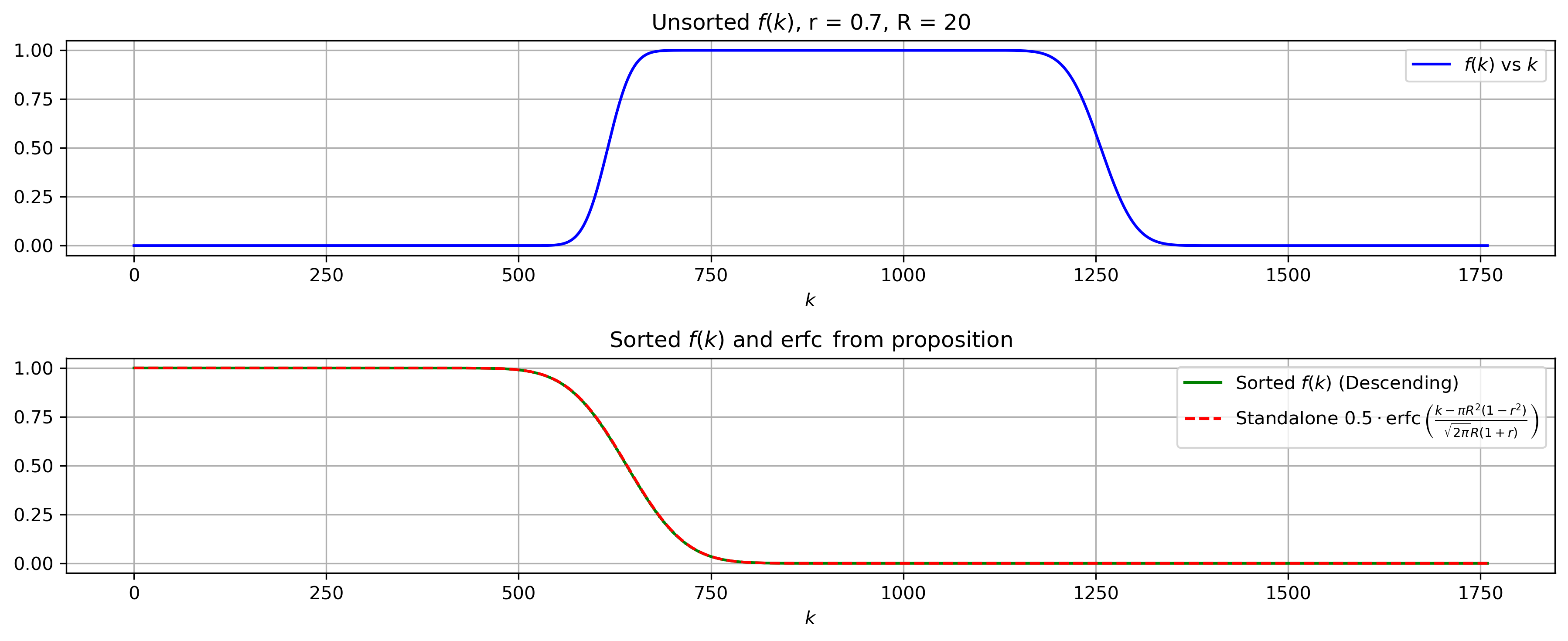
Figure 1. Numerical verification of Proposition 2.2 with $R=20$, $r=0.7$ comparing a manual sorting of samples of $f$ with the proposed $\tilde{f}^{*}$.

The same translation argument we mentioned for disks applies to annuli since the proof is only based on the collection of eigenvalues $(\lambda_{k}^{R})_{k}$.

Our final generalization of this result is a lifting to all rotationally invariant sets with a finite number of connected components. Note that rotationally invariant sets are just unions of annuli which can be seen by e.g. considering that along an axis, a rotationally invariant set is the union of intervals. For technical reasons we must require that the number of annuli is finite so that the distance between two annuli is bounded away from $0$.

Proposition 2.3.

Let $\Omega\subset\mathbb{R}^{2}$ be a compact and rotationally invariant set with a finite number of connected components and $\lambda_{k}^{R\Omega}$ the $k$-th eigenvalue of the localization operator with symbol $R\Omega$. It then holds that

(11) $$\left|\lambda_{k}^{R\Omega}-\frac{1}{2}\operatorname{erfc}\left(\sqrt{2\pi}\frac{k-|R\Omega|}{|\partial R\Omega|}\right)\right|=O\left(\frac{1}{R}\right).$$

Proof.

Note first that a rotationally invariant $\Omega$ is necessarily a union of annuli $\Omega=\cup_{n=1}^{N}\Omega_{n}$ for which $|\Omega|=\sum_{n=1}^{N}|\Omega_{n}|$ and $|\partial\Omega|=\sum_{n=1}^{N}|\partial\Omega_{n}|$. If we let $r_{\textrm{i}}^{n}$ and $r_{\textrm{o}}^{n}$ denote the inner and outer radii of $\Omega_{n}$, we can write the unordered eigenvalues of $A_{\Omega}^{g_{0}}$ as

$$\mu_{k}^{\Omega}=\sum_{n=1}^{N}\lambda_{k}^{r_{\textrm{o}}^{n}}-\lambda_{k}^{r_{\textrm{i}}^{n}}$$

where $\lambda_{k}^{R}$ is $k$-th eigenvalue of $A_{B(0,R)}^{g_{0}}$. If we let $f$ be the function

$$f(x)=\sum_{n=1}^{N}\frac{1}{2}\left(\operatorname{erfc}\left(\frac{x-\pi(r_{\textrm{o}}^{n})^{2}}{\sqrt{2\pi}r_{\textrm{o}}^{n}}\right)-\operatorname{erfc}\left(\frac{x-\pi(r_{\textrm{i}}^{n})^{2}}{\sqrt{2\pi}r_{\textrm{i}}^{n}}\right)\right)=\sum_{n=1}^{N}f_{n}(x),$$

the unordered $\mu_{k}^{\Omega}$ are (asymptotically) samples of $f$ at the integers. We will need for these $f_{n}$ to be orthogonal and to that end set out to construct functions $\tilde{f}_{n}$ which are compactly supported on disjoint subsets of $\mathbb{R}^{+}$. For each $n\geq 1$, define the expanded radii and the set

$$\tilde{r}_{\textrm{i}}^{n}=r_{\textrm{i}}^{n}-\frac{r_{\textrm{i}}^{n}-r_{\textrm{o}}^{n-1}}{2},\qquad\tilde{r}_{\textrm{o}}^{n}=r_{\textrm{o}}^{n}+\frac{r_{\textrm{i}}^{n+1}-r_{\textrm{o}}^{n}}{2},\qquad E_{n}=\big{[}\tilde{r}_{\textrm{i}}^{n},\tilde{r}_{\textrm{o}}^{n}\big{]}$$

where we set $r_{\textrm{o}}^{0}=0$ to treat the edge case. Then if we define the compactly supported functions $\tilde{f}_{n}(x)=\chi_{E_{n}}(x)f_{n}(x)$, it holds that

$$\big{\|}f_{n}-\tilde{f}_{n}\big{\|}_{\infty}=\max\big{\{}f_{n}(\tilde{r}_{\textrm{i}}^{n}),f_{n}(\tilde{r}_{\textrm{o}}^{n})\big{\}}.$$

To see that this quantity is $O(\frac{1}{R})$ when we scale $\Omega$, note that since $\tilde{r}_{\textrm{i}}^{n}<r_{\textrm{i}}^{n}$ and $\tilde{r}_{\textrm{o}}^{n}>r_{\textrm{o}}^{n}$, when we plug these values into $f_{n}$ it will be bounded by $\operatorname{erfc}(\varepsilon R)$ for some $\varepsilon>0$ which is $O(\frac{1}{R})$ by the same expansion from [7, §7.12(i)] we used in Proposition 2.2.

Now using Proposition 2.2, the rearrangement of each $f_{n}$ can be written as

$$f_{n}^{*}(x) =\frac{1}{2}\operatorname{erfc}\left(\frac{x-\pi\big{(}(r_{\textrm{o}}^{n})^{2}-(r_{\textrm{i}}^{n})^{2}\big{)}}{\sqrt{2\pi}(r_{\textrm{o}}^{n}+r_{\textrm{i}}^{n})}\right)+O\left(\frac{1}{|\partial\Omega_{n}|}\right)$$

$$=\frac{1}{2}\operatorname{erfc}\left(\sqrt{2\pi}\frac{x-|\Omega_{n}|}{|\partial\Omega_{n}|}\right)+O\left(\frac{1}{|\partial\Omega_{n}|}\right).$$

Since $\|f_{n}-\tilde{f}_{n}\|_{\infty}=O(\frac{1}{R})$, we can conclude that $\|f_{n}^{*}-\tilde{f}_{n}^{*}\|_{\infty}=O(\frac{1}{R})$. Define

$$g_{n}(x)=\frac{1}{2}\operatorname{erfc}\left(\sqrt{2\pi}\frac{x-|\Omega_{n}|}{|\partial\Omega_{n}|}\right)$$

so that $\|g_{n}-f_{n}^{*}\|_{\infty}=O(\frac{1}{R})$ and, in turn, $\|g_{n}-\tilde{f}_{n}^{*}\|_{\infty}=O(\frac{1}{R})$. If we also define

$$\tilde{f}(x)=\sum_{n=1}^{N}\tilde{f}_{n}(x)\implies\|\tilde{f}^{*}-f^{*}\|_{\infty}=\left\|\sum_{n=1}^{N}(\tilde{f}_{n}-f_{n})\right\|_{\infty}=O\left(\frac{1}{R}\right),$$

we see that it suffices to show that $\|f^{*}-\frac{1}{2}\operatorname{erfc}\big{(}\sqrt{2\pi}\frac{\cdot-|\Omega|}{|\partial\Omega|}\big{)}\|_{\infty}=O(\frac{1}{R})$. Since the collection $(\tilde{f}_{n})_{n}$ all have disjoint supports, we can write

(12) $$|\{x\geq 0:\tilde{f}^{*}(x)>\gamma\}|=\sum_{n=1}^{N}|\{x\geq 0:\tilde{f}_{n}(x)>\gamma\}|=\sum_{n=1}^{N}|\{x\geq 0:\tilde{f}_{n}^{*}(x)>\gamma\}|$$

where we in the last step used that the measures of level sets are unaffected by rearrangements. For the $g_{n}$ functions, we can explicitly compute

$$|\{x\geq 0:g_{n}(x)>\gamma\}|=g_{n}^{-1}(\gamma)=|\Omega_{n}|+\operatorname{erfc}^{-1}(2\gamma)\frac{|\partial\Omega_{n}|}{\sqrt{2\pi}}.$$

Now write $\varepsilon$ for the largest difference between $|\tilde{f}_{n}^{*}-g_{n}|$ over all $n$, it then holds that

$$|\{x\geq 0:g_{n}(x)>\gamma+\varepsilon\}| \leq|\{x\geq 0:\tilde{f}_{n}^{*}(x)>\gamma\}|\leq|\{x\geq 0:g_{n}(x)>\gamma-\varepsilon\}|$$

$$\implies|\Omega_{n}|+\frac{|\partial\Omega_{n}|}{\sqrt{2\pi}}\operatorname{erfc}^{-1}(2(\gamma+\varepsilon)) \leq|\{x\geq 0:\tilde{f}_{n}(x)>\gamma\}|\leq|\Omega_{n}|+\frac{|\partial\Omega_{n}|}{\sqrt{2\pi}}\operatorname{erfc}^{-1}(2(\gamma-\varepsilon))$$

$$\implies|\Omega|+\frac{|\partial\Omega|}{\sqrt{2\pi}}\operatorname{erfc}^{-1}(2(\gamma+\varepsilon)) \leq|\{x\geq 0:\tilde{f}^{*}(x)>\gamma\}|\leq|\Omega|+\frac{|\partial\Omega|}{\sqrt{2\pi}}\operatorname{erfc}^{-1}(2(\gamma-\varepsilon))$$

where we in the last step summed over $n$ and plugged in (12). Equivalently, since $\tilde{f}^{*}$ is decreasing (since no $\tilde{f}_{n}$ has derivative zero in an interval), we can write

$$\tilde{f}^{*}\left(|\Omega|+\frac{|\partial\Omega|}{\sqrt{2\pi}}\operatorname{erfc}^{-1}(2(\gamma+\varepsilon))\right)\leq\tilde{f}^{*}(x)=\gamma\leq\tilde{f}^{*}\left(|\Omega|+\frac{|\partial\Omega|}{\sqrt{2\pi}}\operatorname{erfc}^{-1}(2(\gamma-\varepsilon))\right).$$

Moreover, $\tilde{f}^{*}$ is invertible and so we can conclude that for any $\gamma=\tilde{f}^{*}(x)$,

$$|\Omega|+\frac{|\partial\Omega|}{\sqrt{2\pi}}\operatorname{erfc}^{-1}(2(\gamma+\varepsilon)) \leq(\tilde{f}^{*})^{-1}(\gamma)\leq|\Omega|+\frac{|\partial\Omega|}{\sqrt{2\pi}}\operatorname{erfc}^{-1}(2(\gamma-\varepsilon))$$

$$\implies\operatorname{erfc}^{-1}(2(\gamma+\varepsilon)) \leq\frac{\sqrt{2\pi}}{|\partial\Omega|}\Big{[}(\tilde{f}^{*})^{-1}(\gamma)-|\Omega|\Big{]}\leq\operatorname{erfc}^{-1}(2(\gamma-\varepsilon))$$

$$\implies\gamma-\varepsilon \leq\frac{1}{2}\operatorname{erfc}\left(\frac{\sqrt{2\pi}}{|\partial\Omega|}\Big{[}(\tilde{f}^{*})^{-1}(\gamma)-|\Omega|\Big{]}\right)\leq\gamma+\varepsilon$$

$$\implies\tilde{f}^{*}(x)-\varepsilon \leq\frac{1}{2}\operatorname{erfc}\left(\sqrt{2\pi}\frac{x-|\Omega|}{|\partial\Omega|}\right)\leq\tilde{f}^{*}(x)+\varepsilon.$$

With this we can finish the proof by noting that $\big{|}\lambda_{k}^{R\Omega}-f^{*}(k)\big{|}=O(\frac{1}{R})$ by the same argument as we used in Proposition 2.2 and that $\varepsilon=O(\frac{1}{R})$ since $N$ is finite. ∎

2.2. Universality

These proofs have ultimately led us to the $\operatorname{erfc}$ asymptotics by a central limit theorem argument which notoriously is universal in the sense that we get the same limit for a large class of probability distributions. In physics, the notion of universality [6] near a boundary point is a well studied phenomenon and in particular $\operatorname{erfc}$ universality is a very important result in random matrix theory [14]. This setting is of particular interest due to its strong connection to localization operators, see [4, 1].

An early piece of evidence in the direction of the boundary universality conjecture in random matrix theory [14] was the calculation of the eigenvalue asymptotics for the special case of the Gaussian unitary ensemble (GUE), where each entry in the random matrix is a Gaussian random variable. In this setup, Forrester and Honner [11] showed that the density of the eigenvalues near a boundary point will converge to an $\operatorname{erfc}$ kernel in the limiting case. The Gaussian unitary ensemble precisely corresponds to the case of a localization operator with Gaussian window functions and the disk as its symbol through an intricate procedure involving the Bargmann transform [4]. This correspondence inspires confidence that the link between random matrices and eigenvalues of localization operators may persist in the eigenvalues asymptotics for more general classes of symbols.

It is conceivable that for other $\Omega$ than those we have discussed, there could exist a random variable $X_{\Omega}$ such that $\lambda_{k}^{\Omega}=\mathbb{P}(X_{\Omega}\leq k)$ that has the property that this probability is related to the central limit theorem in the large $R$ limit. To make a precise conjecture on these asymptotics, we first need to make the rescaling implicit in Theorem 2.1, Proposition 2.2 and Proposition 2.3 more explicit. Following the setup in e.g. [3], we define the dilation $R\Omega$ of $\Omega$ as

$$R\Omega=\{z\in\mathbb{R}^{2d}:z/R\in\Omega\ \}.$$

In both (5) and (6), the argument of the $\operatorname{erfc}$ function can be written as

$$\sqrt{2\pi}\frac{k-|R\Omega|}{|\partial R\Omega|}$$

and we conjecture that this behavior could be universal.

Conjecture 2.4.

Let $\Omega\subset\mathbb{R}^{2}$ be compact and $\lambda_{k}^{\Omega}$ be the $k$-th eigenvalue of the localization operator with symbol $\Omega$ and window the standard Gaussian. Then

$$\left|\lambda_{k}^{R\Omega}-\frac{1}{2}\operatorname{erfc}\left(\sqrt{2\pi}\frac{k-|R\Omega|}{|\partial R\Omega|}\right)\right|=O\left(\frac{1}{R}\right)$$

where $\operatorname{erfc}$ is the complementary error function.

In particular, this conjecture implies that the plunge region has width comparable to $|\partial\Omega|$ which is a weaker result which we will investigate in Section 3.

It is possible that we might have to require stronger conditions on $\Omega$ for the conjecture to hold. In particular the condition of $\Omega$ having maximally Ahlfors regular boundary has proven important in recent work by Marceca and Romero [20]. However in the absence of evidence to the contrary, we present the conjecture in full generality.

A reason to believe in plunge profile universality is the min-max formulation of the eigenvalues of $A_{\Omega}^{g}$ discussed in e.g. [3], namely

$$\lambda_{k}^{\Omega}=\max\left\{\int_{\Omega}|V_{g}f(z)|^{2}\,dz:\|f\|_{L^{2}}=1,f\perp h_{1}^{\Omega},\dots,h_{k-1}^{\Omega}\right\}.$$

This implies that the plunge eigenvalues belong to the eigenfunctions which are supported around the boundary of $\Omega$. In particular, the values $\lambda_{k}^{\Omega}$ depend on how the short-time Fourier transforms of orthogonal eigenfunctions $h_{k}^{\Omega}$ repel each other around the boundary. In the large $R$ limit, the boundary $\partial R\Omega$ is approximately straight both for $\Omega=B(0,1)$ and general $\Omega$, save for pathological examples. It is therefore not unreasonable that the eigenfunctions, which do not scale with $R$, would have the same behavior for any $\Omega$ when $R$ is large as these local objects do not sense the global structure of $R\Omega$.

If the window function $g$ induces some form of anisotropy in the time-frequency plane, the number of spectrograms $|V_{g}h_{k}^{\Omega}|^{2}$ which occupy a given stretch of $\partial\Omega$ could be dependent on the angle for this approximate line segment. This is not an issue for the interior, where there are no boundary effects to consider and all spectrograms take up the same area, 1. In [5, Section V.B], it is shown that when the window is a dilated Gaussian and the symbol is a corresponding ellipse, the eigenvalues are the same as for a symmetric disk and the standard Gaussian. Hence, we know that the conjecture is false if we remove the condition of the window being the standard Gaussian. This issue is investigated numerically in Section 3.3 below.

Still, we have so far only presented heuristic arguments in favor of Conjecture 2.4. Our main evidence comes in the form of computing $\lambda_{k}^{\Omega}-\frac{1}{2}\operatorname{erfc}\big{(}\sqrt{2\pi}\frac{k-|\Omega|}{|\partial\Omega|}\big{)}$ for a large collection of $\Omega$ for frame multipliers. The strong correspondence between results for localization operators and Gabor multipliers has been investigated for a long time and holds up well, from proving the same eigenvalue plunge behavior [8, 9] to showing trace-class convergence for dense lattices [10] and accumulated spectrogram behavior [13].

3. Numerical verification

In this section we attempt to verify Conjecture 2.4 numerically using the Large Time-Frequency Analysis Toolbox (LTFAT) [22]. Obviously, we are not able to realize localization operators as they are continuous objects and even Gabor multipliers are based on samples of $L^{2}(\mathbb{R}^{d})$ functions. However, the finite Gabor multipliers, or frame multipliers, we can realize in LTFAT which are based on vector representations of signals are likely to approximate Gabor multipliers well. Moreover, those Gabor multipliers in turn will have similar eigenvalue behavior as the corresponding localization operators as they are close in trace-class and Hilbert-Schmidt norms for dense lattices [10, 9].

3.1. Setup

In LTFAT, the framemuleigs function takes in a symbol, analysis frame and synthesis frame and returns the eigenvalues and optionally the eigenvectors of the corresponding frame multiplier. The frames are in turn determined by the time-hop distance a, the number of frequency channels M and the window function g. To avoid under- and oversampling, we always set the signal length L to $\textsf{L}=\textsf{a}\times\textsf{M}$ and unless stated otherwise, we use a standard Gaussian window function g = pgauss(L).

The full code is available on GitHub and should ideally be self-explanatory. In LTFAT, symbols are defined on a $\textsf{M}\times\textsf{M}$ grid and we have used a pipeline where images can be converted to binary masks to simplify experimentation with symbols which are difficult to define in code. The area $|\Omega|$ is computed by summing the symbol while for the perimeter length $|\partial\Omega|$ we use the built-in MATLAB function regionprops. To account for the different coordinates in discrete phase space, the symbol area is multiplied by a / M and the perimeter by $\sqrt{\textsf{a/M}}$.

To support a weaker version of the conjecture numerically, we will write out the length of the perimeter as reported by regionprops, the number of eigenvalues in the plunge region with $\delta=0.1$ as well as their quotient which should be approximately constant across different symbols and frames.

3.2. Symbol and frame dependence

We will first consider the case which we know best, that where the symbol is a disk. The error we observe here will serve as a benchmark for all upcoming experiments as they should only come from the following factors:

• Finite size symbol (not asymptotic limit),

• Localization operator to Gabor multiplier error (lattice effects),

• Gabor multiplier to frame multiplier error (discrete functions),

• Lattice boundary length (measuring $|\partial\Omega|$ using regionprops).

For this reason, we expect that the errors we observe for the disk should be a lower bound for the errors we observe, a form of noise floor.

Figure 2. Experiment with $\textsf{a}=10,\textsf{M}=100$, Gaussian window and a disk as the symbol. Maximum error is close to $1.0$%.

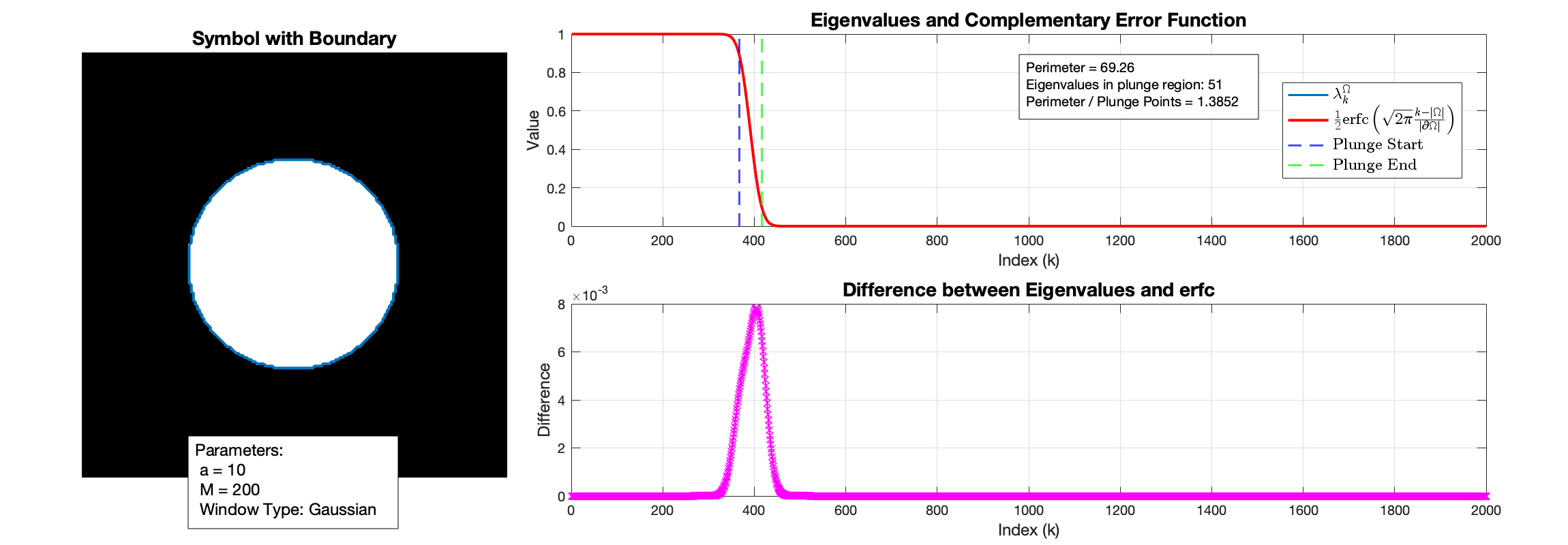
Figure 3. Experiment with $\textsf{a}=10,\textsf{M}=200$, Gaussian window and a disk as the symbol. Maximum error is close to $0.8$%.

The higher value for M corresponds to a denser lattice which explains the smaller peak discrepancy in Figure 3 compared to Figure 2.

Next we look at a collection of different symbols and frame parameters. For a star shape we observe considerably higher errors for a sparse lattice but for the $\textsf{a}=10,\textsf{M}=100$ lattice the error is comparable to that for the disk, see Figures 4 and 5.

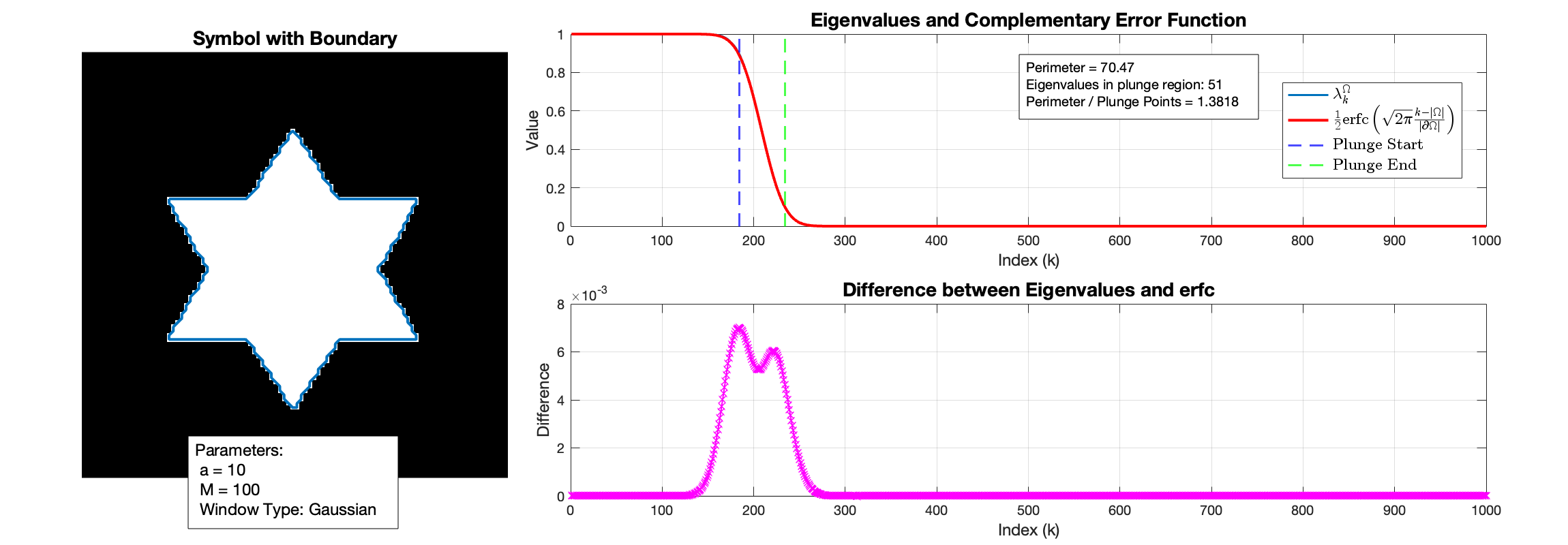
Figure 4. Experiment with $\textsf{a}=10,\textsf{M}=100$, Gaussian window and a star shape as the symbol. Maximum error is close to $0.7$%.

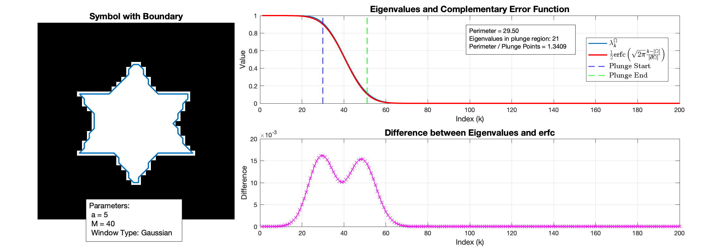
Figure 5. Experiment with $\textsf{a}=5,\textsf{M}=40$, Gaussian window and a star shape as the symbol. Maximum error is close to $1.6$%.

The symbols in Figures 6 and 7 are poorly conditioned as they are thin which means that eigenfunctions belonging to the plunge region are likely to be influenced by the symbol boundary on the opposite side. In this case, we see considerably higher errors.

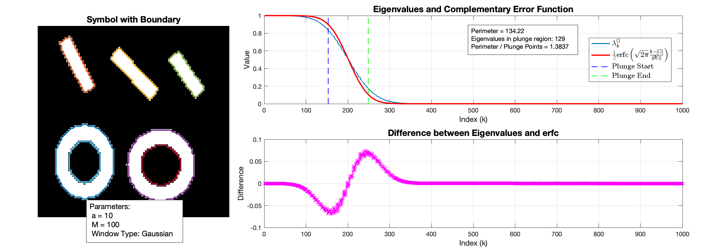
Figure 6. Experiment with $\textsf{a}=10,\textsf{M}=100$, Gaussian window and lines and circles as the symbol. Maximum error is close to $7.5$%.

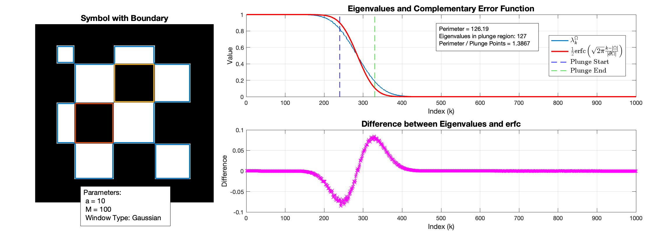
Figure 7. Experiment with $\textsf{a}=10,\textsf{M}=100$, Gaussian window and tiles as the symbol. Maximum error is close to $8.0$%.

For a more well behaved but still intricate symbol, see Figure 8.

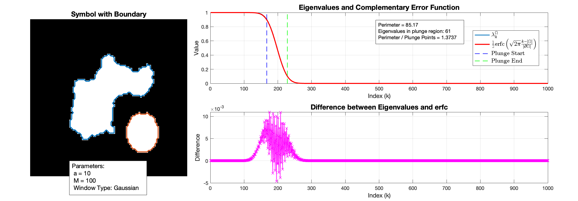
Figure 8. Experiment with $\textsf{a}=10,\textsf{M}=100$, Gaussian window and blobs as the symbol. Maximum error is close to $1.1$%.

The case of elliptical symbols was discussed in [5, Section V.B] where it was shown that if the Gaussian window was dilated appropriately, the eigenvalue behavior is the same as for the disk with the same area. However, the perimeter of an ellipse differs significantly from that of the disk with the same area, which is why we required the window to be the standard Gaussian. In Figure 9, we verify that the conjecture still appears to hold in this case.

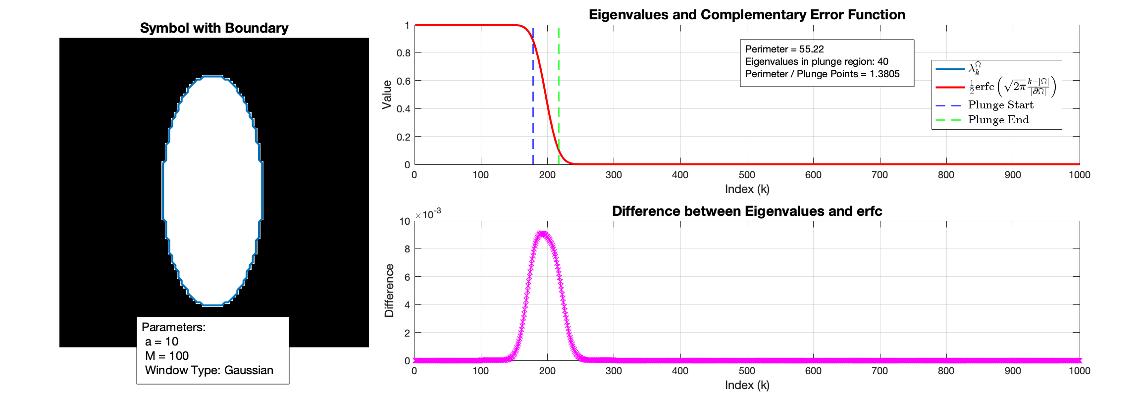
Figure 9. Experiment with $\textsf{a}=10,\textsf{M}=100$, Gaussian window and an ellipse as the symbol. Maximum error is close to $0.9$%.

Lastly we look at a square symbol (Figure 10) where the results are similar to those for the disk or star.

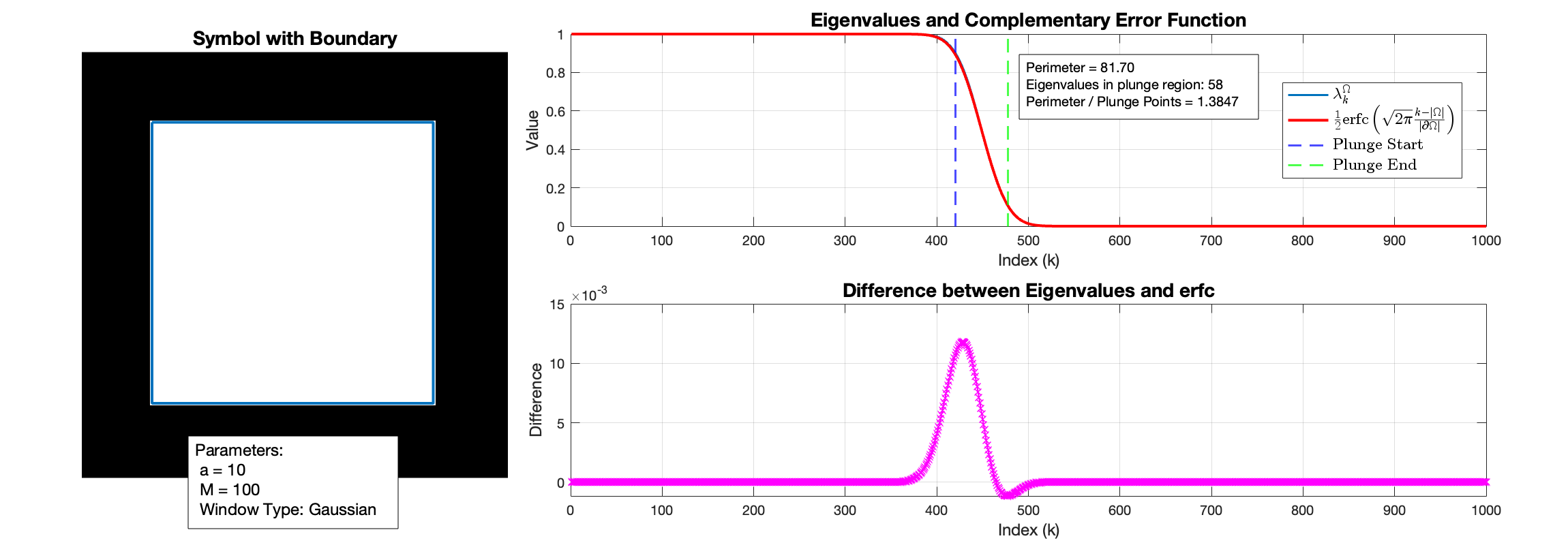
Figure 10. Experiment with $\textsf{a}=10,\textsf{M}=100$, Gaussian window and a square as the symbol. Maximum error is close to $1.2$%.

The results from all the above figures are summarized in Table 1.

Table 1. Summarized results for a collection of symbols and parameters. Here $\#P$ denotes the cardinality of the plunge region with parameter $\delta=0.1$.

Symbol	a	M	$\boldsymbol{L^{\infty}}$ error	$\boldsymbol{|\partial\Omega|/\#P}$
Disk	$10$	$100$	$1.0$%	1.3806
Disk	$10$	$200$	$0.8$%	1.3852
Star	$10$	$100$	$1.0$%	1.3818
Star	$5$	$40$	$1.6$%	1.3409
Lines and circles	$10$	$100$	$7.5$%	1.3837
Tiles	$10$	$100$	$8.0$%	1.3867
Blobs	$10$	$100$	$1.1$%	1.3737
Ellipse	$10$	$100$	$0.9$%	1.3805
Square	$10$	$100$	$1.2$%	1.3847

The tiles and lines and circles examples have considerably higher errors and were chosen to have a high $|\partial\Omega|/|\Omega|$ ratio. For the symbols which are interior-dominated, as all symbols are asymptotically as we scale $R$, the $\operatorname{erfc}$ curve is remarkably close to the true eigenvalue behavior.

3.3. Window dependence

All of the examples we have seen so far have been with a Gaussian window. In this section, we show that the fitted curve has a markedly larger discrepancy when the window is a box function, which has worse time-frequency concentration than the standard Gaussian, and offer an explanation for why.

In Figure 11, we have repeated the experiment from the previous section with a different window and get a noticeably larger discrepancy.

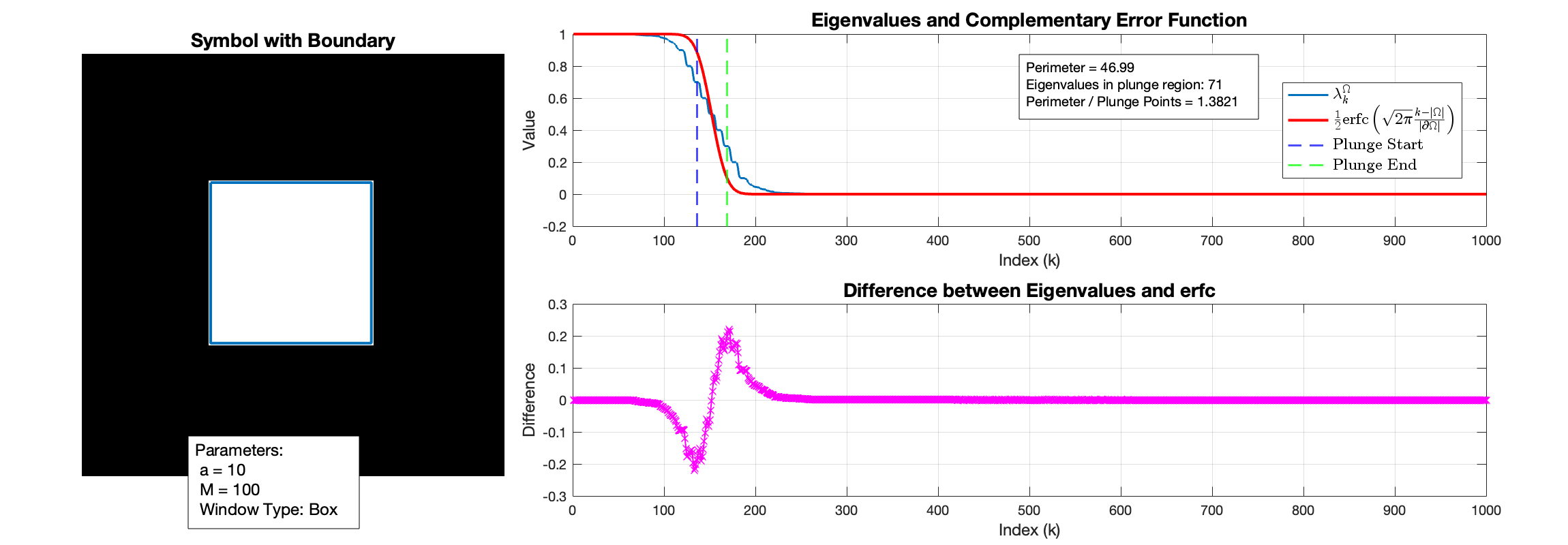
Figure 11. Eigenvalue decay for frame multiplier with box window function.

Other symbols also have similarly uneven decay which is also wider than that for Gaussian windows.

As mentioned near the end of Section 2, we have reason to believe that the spectrograms corresponding to different eigenfunctions are more separated when the window function has uneven concentration in time versus frequency. To investigate this, we consider a sparse time-frequency lattice and a disk symbol. By taking the three spectrograms corresponding to the eigenvalues in the middle of the plunge region, those closest to $\lambda=1/2$, and mapping their brightness to different color channels this separation can be visualized, see Figure 12.

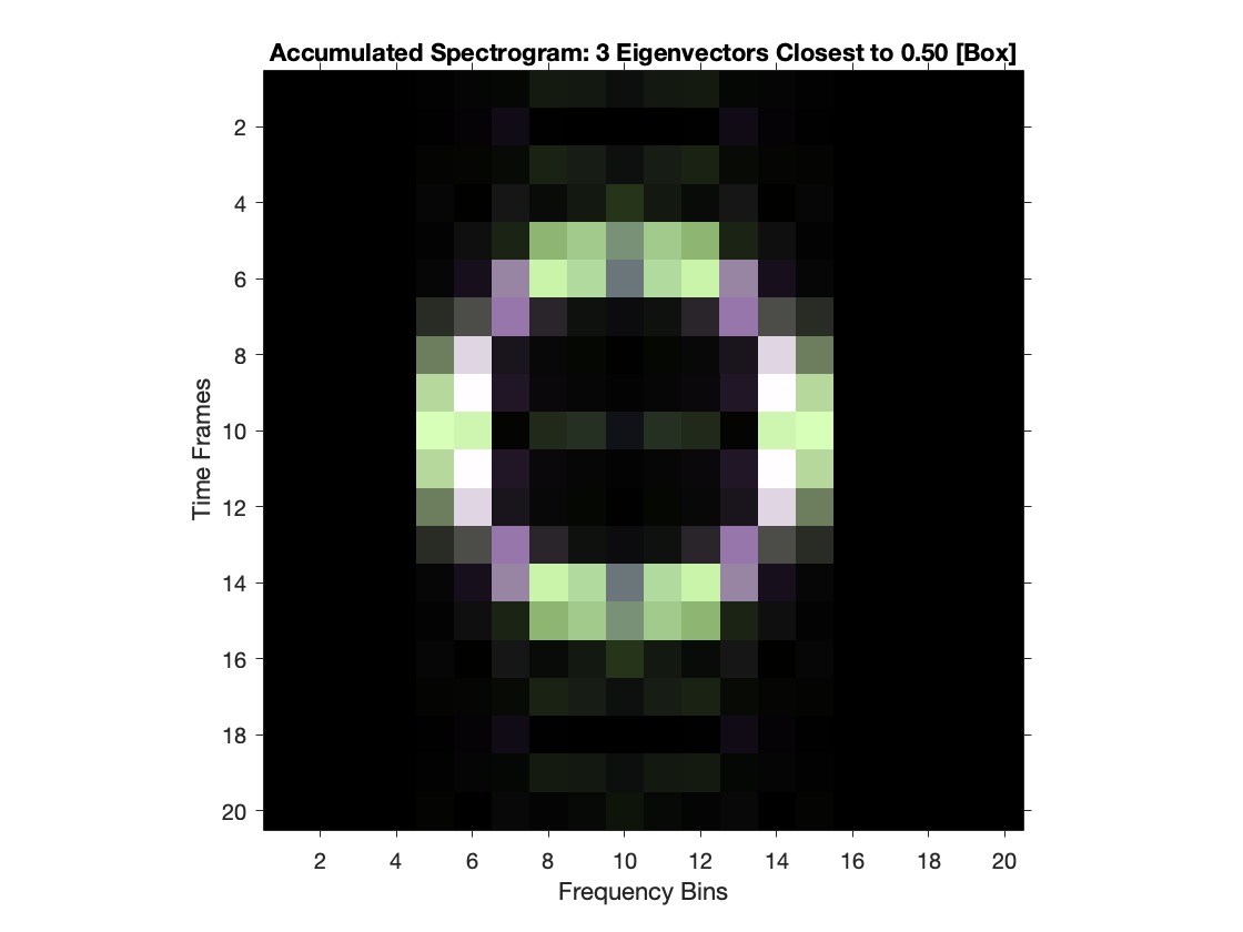
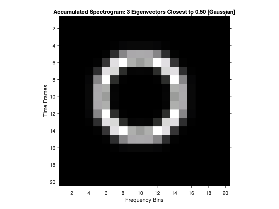
Figure 12. Accumulated spectrograms of three eigenfunctions (colored red, green, blue) closest to eigenvalue $1/2$ for a box window (left) and a Gaussian window (right).

In Figure 12 we see that the accumulated spectrogram with Gaussian window is almost monochrome, meaning that the spectrograms always intersect while the spectrograms with a box window are well separated.

References

- [1] Luis Daniel Abreu, Joao Pereira, Jose Luis Romero and Salvatore Torquato “The Weyl-Heisenberg ensemble: Statistical mechanics meets time-frequency analysis” In 2017 International Conference on Sampling Theory and Applications (SampTA) IEEE, 2017, pp. 199–202 DOI: 10.1109/sampta.2017.8024413
- [2] Luís Daniel Abreu and Monika Dörfler “An inverse problem for localization operators” In Inverse Problems 28.11 IOP Publishing, 2012, pp. 115001 DOI: 10.1088/0266-5611/28/11/115001
- [3] Luís Daniel Abreu, Karlheinz Gröchenig and José Luis Romero “On accumulated spectrograms” In Trans. Amer. Math. Soc. 368.5 American Mathematical Society (AMS), 2015, pp. 3629–3649 DOI: 10.1090/tran/6517
- [4] Luís Daniel Abreu, J M Pereira, J L Romero and S Torquato “The Weyl–Heisenberg ensemble: hyperuniformity and higher Landau levels” In J. Stat. Mech. Theory Exp. 2017.4 IOP Publishing, 2017, pp. 043103 DOI: 10.1088/1742-5468/aa68a7
- [5] I. Daubechies “Time-frequency localization operators: a geometric phase space approach” In IEEE Trans. Inform. Theory 34.4 Institute of ElectricalElectronics Engineers (IEEE), 1988, pp. 605–612 DOI: 10.1109/18.9761
- [6] Percy Deift “Universality for mathematical and physical systems” 25th International Congress of Mathematicians, ICM 2006, 2006, pp. 125–152
- [7] F… Olver et al. “NIST Digital Library of Mathematical Functions”, Release 1.2.3 of 2024-12-15 URL: https://dlmf.nist.gov/
- [8] H.. Feichtinger and K. Nowak “A Szegő-type theorem for Gabor-Toeplitz localization operators” In Michigan Math. J. 49.1, 2001 DOI: 10.1307/mmj/1008719032
- [9] H.. Feichtinger and K. Nowak “A First Survey of Gabor Multipliers” In Advances in Gabor Analysis Boston, MA: Birkhäuser Boston, 2003, pp. 99–128 DOI: 10.1007/978-1-4612-0133-5˙5
- [10] Hans G. Feichtinger, Simon Halvdansson and Franz Luef “Measure-operator convolutions and applications to mixed-state Gabor multipliers” In Sampl. Theory Signal Process. Data Anal. 22.2 Springer ScienceBusiness Media LLC, 2024 DOI: 10.1007/s43670-024-00090-0
- [11] P J Forrester and G Honner “Exact statistical properties of the zeros of complex random polynomials” In J. Phys. A 32.16 IOP Publishing, 1999, pp. 2961–2981 DOI: 10.1088/0305-4470/32/16/006
- [12] K. Gröchenig “Foundations of Time-Frequency Analysis” Birkhäuser Boston, 2001 DOI: 10.1007/978-1-4612-0003-1
- [13] Simon Halvdansson “On accumulated spectrograms for Gabor frames” In J. Math. Anal. Appl. 543.2 Elsevier BV, 2025, pp. 129044 DOI: 10.1016/j.jmaa.2024.129044
- [14] Håkan Hedenmalm and Aron Wennman “Planar orthogonal polynomials and boundary universality in the random normal matrix model” In Acta Math. 227.2 International Press of Boston, 2021, pp. 309–406 DOI: 10.4310/acta.2021.v227.n2.a3
- [15] Aleksei Kulikov “Exponential lower bound for the eigenvalues of the time-frequency localization operator before the plunge region” In Appl. Comput. Harmon. Anal. 71 Elsevier BV, 2024, pp. 101639 DOI: 10.1016/j.acha.2024.101639
- [16] H.. Landau “On Szegö’s eigenvalue distribution theorem and non-Hermitian kernels” In J. Anal. Math. 28.1 Springer ScienceBusiness Media LLC, 1975, pp. 335–357 DOI: 10.1007/bf02786820
- [17] H.. Landau and H.. Pollak “Prolate Spheroidal Wave Functions, Fourier Analysis and Uncertainty - II” In Bell System Tech. J. 40.1 Institute of ElectricalElectronics Engineers (IEEE), 1961, pp. 65–84 DOI: 10.1002/j.1538-7305.1961.tb03977.x
- [18] H.. Landau and H.. Pollak “Prolate Spheroidal Wave Functions, Fourier Analysis and Uncertainty-III: The Dimension of the Space of Essentially Time- and Band-Limited Signals” In Bell System Tech. J. 41.4 Institute of ElectricalElectronics Engineers (IEEE), 1962, pp. 1295–1336 DOI: 10.1002/j.1538-7305.1962.tb03279.x
- [19] Elliott H Lieb and Michael Loss “Analysis”, Graduate studies in mathematics Providence, RI: American Mathematical Society, 2001
- [20] Felipe Marceca and José Luis Romero “Spectral deviation of concentration operators for the short-time Fourier transform” In Studia Math. 270.2 Institute of Mathematics, Polish Academy of Sciences, 2023, pp. 145–173 DOI: 10.4064/sm220214-17-10
- [21] Felipe Marceca, José Luis Romero and Michael Speckbacher “Eigenvalue estimates for Fourier concentration operators on two domains” In Arch. Rat. Mechan. Anal. 248.3 Springer ScienceBusiness Media LLC, 2024 DOI: 10.1007/s00205-024-01979-9
- [22] Z. Průša et al. “The Large Time-Frequency Analysis Toolbox 2.0” In Sound, Music, and Motion, LNCS Springer International Publishing, 2014, pp. 419–442 DOI: 10.1007/978-3-319-12976-1“˙25
- [23] Jayakumar Ramanathan and Pankaj Topiwala “Time–Frequency Localization and the Spectrogram” In Appl. Comput. Harmon. Anal. 1.2 Elsevier BV, 1994, pp. 209–215 DOI: 10.1006/acha.1994.1008
- [24] D. Slepian “Prolate Spheroidal Wave Functions, Fourier Analysis, and Uncertainty-V: The Discrete Case” In Bell System Tech. J. 57.5 Institute of ElectricalElectronics Engineers (IEEE), 1978, pp. 1371–1430 DOI: 10.1002/j.1538-7305.1978.tb02104.x
- [25] D. Slepian and H.. Pollak “Prolate Spheroidal Wave Functions, Fourier Analysis and Uncertainty - I” In Bell System Tech. J. 40.1 Institute of ElectricalElectronics Engineers (IEEE), 1961, pp. 43–63 DOI: 10.1002/j.1538-7305.1961.tb03976.x
- [26] David Slepian “Prolate Spheroidal Wave Functions, Fourier Analysis and Uncertainty - IV: Extensions to Many Dimensions; Generalized Prolate Spheroidal Functions” In Bell System Tech. J. 43.6 Institute of ElectricalElectronics Engineers (IEEE), 1964, pp. 3009–3057 DOI: 10.1002/j.1538-7305.1964.tb01037.x