Streamlining Equal Shares

Abstract

Participatory budgeting (PB) is a form of citizen participation that allows citizens to decide how public funds are spent. Through an election, citizens express their preferences on various projects (spending proposals). A voting mechanism then determines which projects will be approved. The Method of Equal Shares (MES) is the state of the art algorithm for a proportional, voting based approach to participatory budgeting and has been implemented in cities across Poland and Switzerland. A significant drawback of MES is that it is not exhaustive meaning that it often leaves a portion of the budget unspent that could be used to fund additional projects. To address this, in practice the algorithm is combined with a completion heuristic - most often the “add-one" heuristic which artificially increases the budget until a heuristically chosen threshold. This heuristic is computationally inefficient and will become computationally impractical if PB is employed on a larger scale. We propose the more efficient add-opt heuristic for Exact Equal Shares (EES), a variation of MES that is known to retain many of its desirable properties. We solve the problem of identifying the next budget for which the outcome for EES changes in $O(mn)$ time for cardinal utilities and $O(m^{2}n)$ time for uniform utilities, where $m$ is the number of projects and $n$ is the number of voters. Our solution to this problem inspires the efficient add-opt heuristic which bypasses the need to search through each intermediary budget. We perform comprehensive experiments on real-word PB instances from Pabulib and show that completed EES outcomes usually match the proportion of budget spent by completed MES outcomes. Furthermore, the add-opt heuristic matches the proportion of budget spend by add-one for EES.

1 Introduction

Participatory budgeting is a democratic process that enables citizens to decide how public funds should be spent. A natural tool for this task is voting: the governing body (e.g., a city) runs an election to gather citizens’ preferences on various projects and uses a voting mechanism to decide how to allocate the funds. The projects offered for a public vote are specific proposals that come with predetermined scope and cost, made publicly known before the election, e.g., “Build a cycle lane on Main Street.". So, rather than electing representatives who make budgetary decisions, citizens vote directly on specific proposals. Today, participatory budgeting is used worldwide in hundreds of cities [De Vries et al., 2022, Wampler et al., 2021] as well as in decentralized autonomous organizations (DAOs) [Wang et al., 2019, Chohan, 2017], which are blockchain-based self-governed communities. For example, in community funding, members can contribute funds to the DAO and then vote on which projects the funds should be granted to.

A commonly used, naive approach to determine which projects should be funded is Greedy Approval (GrA): projects are selected in descending order of votes, skipping those that exceed the remaining budget. However, GrA can be unfair: if 51% of voters support enough projects to exhaust the entire budget, they effectively control 100% of the budget, leaving the remaining 49% of voters unrepresented, whereas ideally, if 10% of citizens vote for, say, cycling-related projects, approximately 10% of the budget should be allocated to the cycling infrastructure. This issue is addressed by the Method of Equal Shares (MES), which is a state-of-the-art voting rule for participatory budgeting this provides representation guarantees to groups of voters with shared preferences [Peters and Skowron, 2020]. In a behavioral experiment by Yang et al. [2024] voters consistently found the outcomes of MES to be fairer than those of GrA. MES has been successfully implemented in Świecie and Wieliczka in Poland, in Aarau and Winterthur in Switzerland, as well as Assen in the Netherlands [Peters and Skowron, 2023].

To overcome the limitations of GrA, MES adopts a market-based approach: The budget is split evenly among all voters, and, for a project to be selected, it must be funded by voters who support it, with all voters paying the same amount (with a caveat that if a voter cannot afford to pay their share, they can contribute their entire remaining budget instead). This limits how much of the budget any group of voters can control. Like GrA, MES selects the projects sequentially; however, in contrast to GrA, the projects are ranked based on the utility per unit of money paid by each fully contributing voter. This twist turns out to capture proportionality as defined by the axiom of Extended Justified Representation (EJR) [Aziz et al., 2017, Peters et al., 2021b], which ensures that each group of voters with shared preferences holds voting power proportional to its size.

A shortcoming of MES is that it often terminates when the leftover budget is large enough to pay for projects that remained unfunded [Peters and Skowron, 2023]. Consequently, MES is said to be non-exhaustive. This underspending is undesirable: indeed, citizens are unhappy when leftover funds could have been used to finance projects they voted for, and many governments have a “use it or lose it” policy, where underspending results in subsequent budgets being cut. This often leads to low-value projects being funded when excess budget is available Liebman and Mahoney [2017]. To mitigate the issue of underspending, the base MES algorithm is supplemented with a heuristic, known as a completion method, to complete the MES outcome.

The strategy currently used in practice is to run MES with a virtual budget that is larger than the actual budget; the size of the virtual budget is selected so that the method spends a larger fraction of the actual budget (but does not exceed it). This strategy is appealing because it does not increase the conceptual complexity of the method: all voters still have equal voting power and, as before, the most cost-efficient projects are selected to be funded, until voters run out of money. In contrast, combining MES with a different algorithm (such as, e.g., GrA) would be harder to explain to the stakeholders, and therefore less appealing in practice.

The challenge, then, is how to determine the “correct” virtual budget. The commonly used add-one heuristic iteratively increases each voter’s budget by one until either (1) the solution becomes exhaustive or (2) the true budget is exceeded, and then returns the last feasible solution. However, this approach is computationally expensive: it often produces identical outcomes across most budget increments [Kraiczy and Elkind, 2023], thereby wasting computational resources. This is especially relevant in the context of research that simulates the method on random instances, as achieving statistical significance requires many repetitions. Importantly, MES has only been employed in smaller communities so far; the add-one heuristic may be infeasible for large cities or DAOs. Another difficulty with the add-one heuristic is the non-monotonicity of MES: MES may overspend at a virtual budget of $b$, but then produce a feasible solution at $b^{\prime}>b$. This means that the add-one method could terminate early and miss the virtual budget that would spend the highest fraction of the budget. Figure˜1 shows a real-life example of this phenomenon. Perhaps even more importantly, even if the costs of all projects are integer, the optimal virtual budget may be non-integer, so add-opt may skip over the optimal virtual budget. Indeed, our analysis in Section 6 shows that for a non-trivial number of real-life instances there are outcomes that can only be achieved by a fractional budget.

Relatedly, the complexity of finding the optimal virtual budget under MES remains unknown. It is not even clear if the associated decision problem (given a value $b^{\prime}\leq b$, determining if there is a virtual budget $b^{*}$ such that MES with budget $b^{*}$ spends at least $b^{\prime}$) is in NP: while $b^{*}$ can be assumed to be rational: due to its sequential nature, MES may potentially produce numbers with super-polynomial bit complexity.

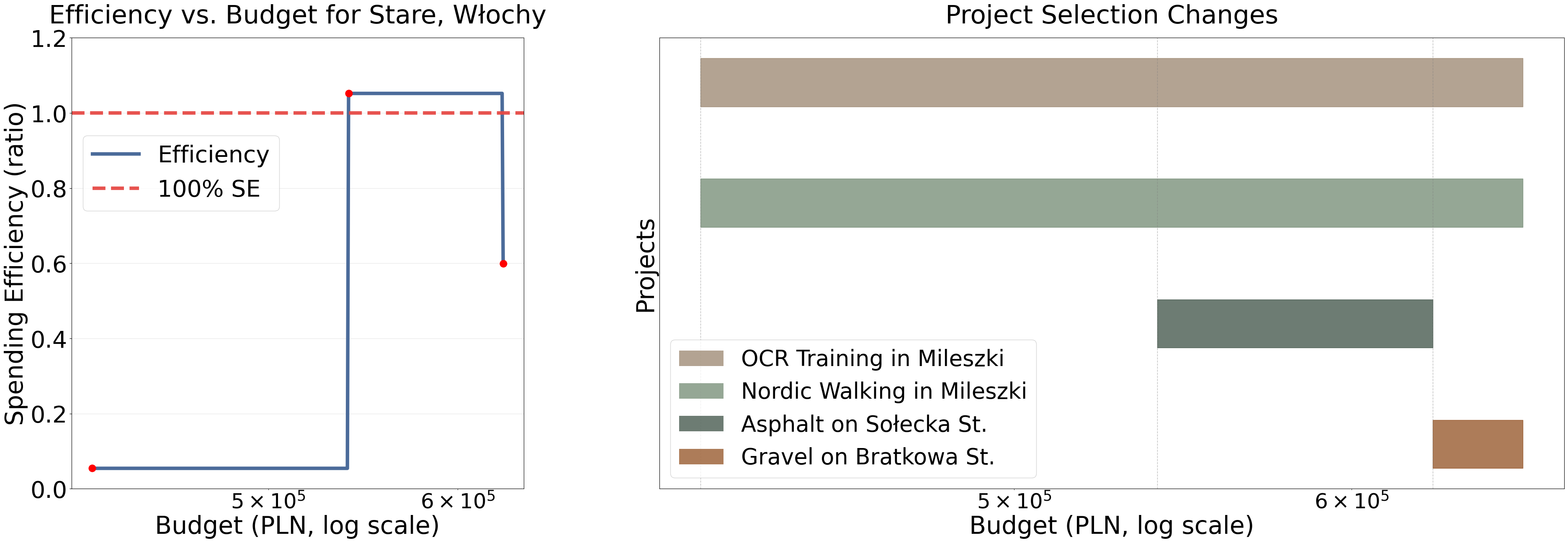
Figure 1: A real-world example where considering all budgets significantly increases spending efficiency, i.e., the fraction of the actual budget spent. The graph on the left shows the spending efficiency of the winning project set for a given virtual budget. The graph on the right shows which projects are selected for a given virtual budget. Here, the add-one heuristic stops as soon as the budget is exceeded, which happens when the Asphalt project is selected. This leads to less than 15% spending efficiency. Increasing the budget further leads to the Asphalt project being dropped in favor of the Gravel project, as depicted on the right, increasing the spending efficiency to 60%

1.1 Contribution

We consider a simplified variant of MES, which we call the Exact Equal Shares (EES) method. Under this rule, all voters who contribute to a project pay exactly the same amount (eliminating the caveat that the voters who are about to run out of money are allowed to contribute their entire budget); we will explain the differences between the two methods in Section 3. This rule was implicit in the work of Peters et al. [2021a] and Kraiczy and Elkind [2023], whose results imply that it retains desirable proportionality properties of MES, but neither paper explicitly defines it.

The simplicity of EES enables us to propose a more principled and efficient approach to finding a good virtual budget. Our main theoretical contribution is a completion method add-opt for EES, which finds the minimum per-voter budget increase that results in changing the set of selected projects or the set of voters paying for a project. The runtime of add-opt is linear in the number of voters $n$. More specifically, for cardinal utilities (i.e., when we evaluate the projects assuming that each voter derives one unit of utility from each selected project they approve), its runtime is $O(mn)$, whereas for the more general model of uniform utilities defined in Section 3 (which subsumes, e.g., cost utilities Peters et al. [2021b]), its runtime is $O(m^{2}n)$.

By using add-opt, we can iterate through all outcomes that can be accomplished by running EES with a virtual budget, and thereby ensure that we do not miss the optimal virtual budget; on the other hand, in contrast to add-one, add-opt avoids redundant computation. Another advantage of add-opt over add-one is that it is currency agnostic, i.e., the results remain consistent across currencies. In contrast, when using add-one, the practitioners need to decide what is an appropriate unit of currency: this choice is non-trivial as, e.g., one US dollar is approximately equal to 16,000 Indonesian rupiahs.

The add-opt heuristic goes through all projects (including ones currently selected), and checks if, by increasing the virtual budget, it can increase the number of voters contributing to that project. While considering all projects is important for ensuring that the optimal virtual budget is not missed, we can achieve faster runtime by only considering projects that are not currently selected; we refer to the resulting heuristic as add-opt-skip.

In order to evaluate the performance of EES with add-opt and add-opt-skip, we perform extensive experiments on real-life participatory budgeting instances. Our results indicate that, on average, EES with add-opt-skip spends the same proportion of the budget as MES with add-one while enjoying far higher computational efficiency and eliminating counterintuitive phenomena such as the one illustrated in Figure˜1.

Complete proofs of results marked by $\spadesuit$ are deferred to Appendix˜A.

1.2 Related Work

Much of the progress in participatory budgeting has built on prior work in multiwinner voting, i.e., a special case of participatory budgeting with unit costs [Lackner and Skowron, 2023]. The Extended Justified Representation (EJR) axiom was first introduced in this context by Aziz et al. [2017].

Besides MES, Phragmén’s method [Phragmén, 1894] and Proportional Approval Voting (PAV) [Thiele, 1895] are well-established proportional rules in the multiwinner voting setting; Janson [2016] provides an excellent overview. PAV satisfies EJR [Aziz et al., 2017] and has optimal proportionality degree, but is NP-hard to compute. Its threshold-based local search variant is polynomial-time computable [Aziz et al., 2018, Kraiczy and Elkind, 2024], but may be hard to explain to voters. Phragmén’s sequential method is also market-based. Unlike MES, it is exhaustive, but it does not satisfy EJR. Moreover, while Peters et al. [2021b] extended MES to participatory budgeting with general additive utilities, neither PAV nor Phragmén have been adapted to this general setting.

Exact Equal Shares for cardinal utilities was implicitly studied by Peters et al. [2021a] and Kraiczy and Elkind [2023]. Peters et al. [2021a] introduce a stability notion for participatory budgeting that is satisfied by the outcome of Exact Equal Shares. Kraiczy and Elkind [2023] propose an adaptive version of EES for cardinal utilities, which uses the outcome of EES for a smaller budget to compute the outcome of EES for a larger budget more efficiently, an alternative approach that complements our work. They also consider the problem of finding the minimum budget increment that changes the election outcome, and propose an $O(n^{2}m)$ algorithm for this problem in the context of cardinal utilities. However, in practice, both in cities and in DAOs, the number of voters ($n$) is usually large, while the number of projects ($m$) is relatively small. As EES itself has a linear dependency on $n$, a completion method with quadratic dependency on $n$ is undesirable.

2 Preliminaries

For each $t\in\mathbb{N}$, we write $[t]=\{1,2,\ldots,t\}$.

Participatory Budgeting (PB)

We first introduce the model of participatory budgeting with cardinal ballots. An election is a tuple $E(b)=(N,P,\{A_{i}\}_{i\in N},{\mathit{cost}},b)$, where:

1. $b\in\mathbb{Q}_{\geq 0}$ is the available budget;

2. $P=\{p_{1},\ldots,p_{m}\}$ is the set of projects; for the purposes of tie-breaking, we fix a total order $\lhd$ on $P$, and write $p=\max Q$ for $Q\subseteq P$ whenever $p^{\prime}\lhd p$ for all $p^{\prime}\in Q\setminus\{p\}$.

3. $N=[n]$ is the set of voters, and for each $i\in N$ the set $A_{i}\subseteq P$ is the ballot of voter $i$;

4. ${\mathit{cost}}:P\rightarrow\mathbb{Q}_{\geq 0}$ is a function that for each $p\in P$ indicates the cost of selecting $p$. For each $Q\subseteq P$, we denote the total cost of $Q$ by ${\mathit{cost}}(Q)=\sum_{p\in Q}{\mathit{cost}}(p)$.

Given a project $p\in P$, we write $N_{p}=\{i\in N\mid p\in A_{i}\}$ for the set of voters who approve $p$. An outcome for an election $E(b)$ is a set of projects $W\subseteq P$ that is feasible, i.e., satisfies ${\mathit{cost}}(W)\leq b$. Our goal is to select an outcome based on voters’ ballots. An aggregation rule (or, in short, a rule) is a function ${{\mathcal{R}}}$ that for each election $E$ selects a feasible outcome ${{\mathcal{R}}}(E)=W$.

Utility Models

We assume that voters’ utilities are induced by a uniform utility function $u:P\rightarrow\mathbb{Q}_{\geq 0}$ so that the utility of a voter $i\in N$ for a project $p\in P$ is given by $u_{i}(p)=u(p)\cdot\mathbb{I}[p\in A_{i}]$, where $\mathbb{I}$ is the indicator function. Important special cases are $u(p)\equiv 1$ (cardinal utilities) and $u(p)={\mathit{cost}}(p)$ for all $p\in P$ (cost utilities). For each $T\subseteq P$ we write $u(T)=\sum_{p\in T}u(p)$ and $u_{i}(T)=\sum_{p\in T}u_{i}(p)$.

Price System

A price system for an outcome $W$ in an election $E(b)=(N,P,\{A_{i}\}_{i\in N},{\mathit{cost}},b)$ is a collection of nonnegative rational numbers $X=(x_{i,p})_{i\in N,p\in P}$, where $x_{i,p}$ denotes voter $i$’s payment for project $p$, satisfying the following three conditions:

• Every voter spends at most her share of the budget: $\sum_{p\in W}x_{i,p}\leq\frac{b}{n}$.

• For each project $p\in W$, the sum of payments towards $p$ equals its cost: $\sum_{i\in N}x_{i,p}={\mathit{cost}}(p)$ for all $p\in W$.

• Voters can only pay for projects they approve: for each $i\in N$ if $x_{i,p}>0$ then $p\in W\cap A_{i}$.

Note that our definition of a price system is less demanding than that of Peters and Skowron [2020], who additionally require that for each project in $P\setminus W$ its supporters do not have enough money left to pay for it.

If $W$ is an outcome for $E(b)$ and $X$ is a price system for $W$, we call the pair $(W,X)$ a solution for $E(b)$. Let $N_{p}(X)=\{i\in N\mid x_{i,p}>0\}$ be the set of voters who pay for $p$ in $X$. We define $O_{p}(X)=N_{p}\setminus N_{p}(X)$ to be the subset of voters who approve $p$, but do not pay for it in $X$. Also, let $r_{i}=\frac{b}{n}-\sum_{p\in P}x_{i,p}$ denote voter $i$’s leftover budget. We say that $X$ is equal-shares if for each $p\in W$ and all $i,j\in N_{p}(X)$ we have $x_{i,p}=x_{j,p}$: that is, the voters who pay for $p$ share the cost of $p$ exactly equally. In this case, we also say that the solution $(W,X)$ is equal-shares.

3 Exact Equal Shares Method

Peters et al. [2021a] and Kraiczy and Elkind [2023] study a variant of MES, which we will call Exact Equal Shares (EES). While they only define EES for cardinal utilities, we will now extend their definition to uniform utilities.

Description

Given an election $E(b)$, EES starts by allocating each voter a budget of $\frac{b}{n}$ and setting $W=\varnothing$. It then iteratively identifies the set of all projects $p\in P\setminus W$ such that a subset of voters $V\subset N_{p}$ have enough leftover budget to split the cost of $p$ equally (i.e., by paying ${\mathit{cost}}(p)/|V|$ each), selects a project in this set with the maximum bang per buck $\frac{u(p)}{\nicefrac{{{\mathit{cost}}(p)}}{{|V|}}}$, adds it to $W$ and updates the budgets. We assume that ties are broken according to the order $\lhd$ on $P$ (see Algorithm˜1 for the pseudocode). We write $\mathit{EES}(E(b),u)$ for the solution $(W,X)$ returned by EES when run on the election $E(b)$ with uniform utility function $u$. For cardinal utilities we will simply write $\mathit{EES}(E(b))$, and for cost utilities we will write $\mathit{EES}(E(b),{\mathit{cost}})$.

The standard Method of Equal Shares (which we refer to as MES) operates similarly, with one exception: if a voter $i$ approves a project, but cannot afford to pay as much as the other contributors, she is allowed to help by contributing her entire leftover budget $r_{i}$. The order in which projects are selected is nevertheless computed based on the contributions of fully paying voters. A detailed description of MES is provided by Peters et al. [2021b].

Input: $E(b)=(N,P,\{A_{i}\}_{i\in N},{\mathit{cost}},b)$, $u:P\rightarrow\mathbb{Q}_{\geq 0}$

Output: Solution $(W,X)$

1 $W$ = $\varnothing$, $X$ = $\textbf{0}^{n\cdot m}$, $r_{i}$ = $\frac{b}{n}$ for all $i\in N$ ;

2 while true do

3    $\Phi$ = $\left\{(p\in P\!\setminus\!W,V\subseteq N_{p})\mid r_{i}\geq\frac{{\mathit{cost}}(p)}{|V|}\quad\forall i\in V\right\}$;

4    if $\Phi=\varnothing$ then

5      return $(W,X)$

6       end if

7      else

8          Let $\Phi^{*}=\operatorname*{arg\,max}_{(p,V)\in\Phi}\frac{|V|\cdot u(p)}{{\mathit{cost}}(p)}$;

9          Choose $(p^{*},V^{*})$ from $\Phi^{*}$ so that $p^{*}\lhd p$ for all $(p,V)\in\Phi^{*}\setminus\{(p^{*},V^{*})\}$;

10         $W$ = $W\cup\{p^{*}\}$;

11          $x_{i,p^{*}}$ = $\frac{{\mathit{cost}}(p^{*})}{|V^{*}|}$, $r_{i}$ = $r_{i}-\frac{{\mathit{cost}}(p^{*})}{|V^{*}|}\quad\forall i\in V^{*}$;

12          end if

13         

14          end while

ALGORITHM 1 EES for uniform utilities

Proportionality Guarantees

A key feature of MES is that for cardinal utilities is satisfies a strong proportionality axiom known as Extended Justified Representation (EJR). We will now formulate this axiom and its relaxation EJR1, and argue that EES is just as attractive as MES from this perspective.

Definition 3.1 (Extended Justified Representation).

Given an election $E(b)=(N,P,\{A_{i}\}_{i\in N},{\mathit{cost}},b)$ and a subset of projects $T\subseteq P$, we say that a group of voters $V$ is $T$-cohesive if $T\subseteq\cap_{i\in V}A_{i}$ and $\frac{|V|}{n}\cdot b\geq{\mathit{cost}}(T)$.

An outcome $W$ for $E(b)$ is said to provide Extended Justified Representation (EJR) (respectively, Extended Justified Representation up to one project (EJR1)) for uniform utilities $u$ if for each $T\subseteq P$ and each $T$-cohesive group $V$ of voters there exists a voter $i\in V$ such that $u_{i}(W)\geq u(T)$ (respectively, $u_{i}(W\cup\{p\})\geq u(T)$ for some $p\in T\setminus W$).

A rule ${{\mathcal{R}}}$ satisfies EJR (respectively, EJR1) if for each election $E(b)$ the outcome ${{\mathcal{R}}}(E(b))$ provides EJR (respectively, EJR1).

Peters and Skowron [2020] show that MES satisfies EJR for cardinal utilities, and the results of Peters et al. [2021a] and Kraiczy and Elkind [2023] imply that the same is true for EES. In contrast, Peters et al. [2021b] show that finding an outcome that satisfies EJR is NP-hard for uniform utilities (they reduce from Knapsack, and construct an election with a single voter, so the utilities are clearly uniform), but MES satisfies EJR1 in an even more general model, which encompasses uniform utilities (namely, arbitrary additive utilities). For completeness, we give a simple proof that EES, too, satisfies EJR1 for uniform utilities (Appendix˜A).

Theorem 3.2.

EES satisfies EJR1 for uniform utilities.

Thus, in the model we consider, EES offers the same proportionality guarantees as MES.

Fast Implementation

Kraiczy and Elkind [2023] show how to implement EES with cardinal utilities in time $O(m^{2}n)$. We will now argue that their approach can be used to guarantee the same runtime for EES with uniform utilities.

Let $R_{t}$, $t\geq 0$, be the list of pairs $(r^{t}_{i},i)_{i\in N}$, where $r^{t}_{i}$ is the leftover budget of voter $i$ after $t$ projects have been bought, sorted in non-decreasing order of first components. As every voter starts off with a budget of $\frac{b}{n}$, we can set $R_{0}=\left((\frac{b}{n},i)_{i\in N}\right)$.

To choose the $(t+1)$-st project, i.e., an as yet unselected project with the highest bang per buck, for each unselected project $p$ we make a single pass through the sorted list $R_{t}$ in order to identify the smallest index $j$ such that the $j$-th entry $(r,i)$ in $R_{t}[N_{p}]$ satisfies $r\geq\frac{{\mathit{cost}}(p)}{|N_{p}|-j+1}$. The value of $j$ determines the bang per buck offered by $p$; we let $p_{t+1}$ be the project with the highest bang per buck, and let $V_{t+1}$ be the set of voters who pay for $p_{t+1}$.

We will now explain how to quickly compute $R_{t+1}$ given $R_{t}$. Suppose each voter in $V_{t+1}$ pays $\delta_{t+1}$. Then, at step $t+1$ the budgets of voters in $V_{t+1}$ are reduced by $\delta_{t+1}$, while the budgets of voters in $N\setminus V_{t+1}$ remain unchanged. Given the list $R_{t}$ and the set $V_{t+1}$, in a singe pass over $R_{t}$ we can create sorted lists $R_{t}[N\setminus V_{t+1}]$ and $R_{t}[V_{t+1}]-\delta_{t+1}$. These two sorted lists can then be merged into $R_{t+1}$ in time $O(n)$. Since this computation has to be done at most $m$ times, it only contributes $O(mn)$ to the overall runtime of the algorithm.

Since the algorithm keeps track of the leftover budgets list, it can easily return this as auxiliary information; this will be relevant in Sections 4 and 5.

4 Towards an Efficient Completion Method for Cardinal Utilities

Our new completion method for EES relies on solving the following computational problem, which we call add-opt: Given the outcome of EES for budget $b$, compute the minimum value of $d$ such that if every voter gets additional budget $d$, EES returns a different outcome, in the sense that the set of selected projects changes or some project is paid for by more voters (or both).

A key to our approach is solving a subproblem concerning a notion of stability for equal-shares solutions, where stability is understood as resistance to deviations by groups of voters. Here we define stability for cardinal utilities in the spirit of Peters et al. [2021a] and Kraiczy and Elkind [2023]; we give a generalization to uniform utilities in Section˜5.

For cardinal utilities, the intuition is as follows. Given a solution $(W,X)$, voter $i$ can deviate from it by contributing her leftover budget $r_{i}$ to support further projects in $A_{i}$. Moreover, even if $i$ does not have enough budget left to contribute to new projects, she may still deviate by withdrawing her support from a project in $W$ and reallocating it to a more cost-efficient project.

Formally, the leximax payment of a voter $i\in N$ in a solution $(W,X)$ is the pair $c_{i}=(x_{i},p_{i})$, where $x_{i}=\max\{x_{i,p}\mid p\in P\}$ and $p_{i}=\max\{p\mid x_{i,p}=x_{i}\}$.We say that $x_{i}$ and $p_{i}$ are the leximax budget and the leximax project of voter $i$, respectively. Given two pairs $(x,p),(x^{\prime},p^{\prime})\in{\mathbb{Q}}\times P$, we write $(x,p)<_{\textit{lex}}(x^{\prime},p^{\prime})$ if $x<x^{\prime}$ or $x=x^{\prime}$ and $p\lhd p^{\prime}$. Given a solution $(W,X)$, we say that voter $i$ is willing to contribute $x$ to $p$ if $x\leq r_{i}$ or $(x,p)<_{\textit{lex}}c_{i}$. Note that voter $i$’s leftover budget $r_{i}$ and her leximax budget $x_{i}$ serve as two distinct sources of funds that $i$ can use to deviate.

Definition 4.1.

A pair $(p,V)$ with $p\in P$, $V\subseteq N_{p}$ certifies the instability of an equal-shares solution $(W,X)$ for an election $E(b)$ if $|V|>|N_{p}(X)|$ and each voter $i\in V\setminus N_{p}(X)$ is willing to contribute $\nicefrac{{{\mathit{cost}}(p)}}{{|V|}}$ to $p$. A project $p\in P$ certifies the instability of an equal-shares solution $(W,X)$ for election $E(b)$ if there exists a set of voters $V_{p}\subseteq N_{p}$ such that $(p,V_{p})$ certifies the instability of $(W,X)$ for $E(b)$. An equal-shares solution $(W,X)$ for $E(b)$ is stable if there is no project $p\in P$ that certifies the instability of $(W,X)$.

This concept of stability captures the behavior of EES, as formalized by the following proposition.

Proposition 4.2 ($\spadesuit$).

EES returns a stable outcome.

We are now ready to state our key subproblem, GreedyProjectChange: Given an election $E(b)=(N,P,\{A_{i}\}_{i\in N},{\mathit{cost}},b)$, a solution $(W,X)$ for election $E(b)$ (along with some auxiliary information), and a project $p$, compute the minimum budget increase $d$ such that project $p$ certifies the instability of $(W,X)$ for $E(b+dn)$.

4.1 GreedyProjectChange for Cardinal Utilities

A simple $O(n^{2})$ solution to GreedyProjectChange [Kraiczy and Elkind, 2023] proceeds by iterating over all values $t=|N_{p}(X)|+1,\ldots,|N_{p}|$ and, for each voter $i\in N_{p}$, calculating the additional budget $d$ that would enable $i$ to contribute $\frac{{\mathit{cost}}(p)}{t}$ towards project $p$. However, we aim for a solution that is linear in $n$, as in practice the number of voters is large, while the number of projects is small.

Intuition

As a a warm-up, consider a set of customers $[n]$ with budgets $\beta_{1}\leq\dots\leq\beta_{n}$ interested in jointly purchasing a service that costs $c$; the costs of the service have to be shared equally by all participating customers. It is well-known how to identify the largest group of customers that can share the cost of the service: it suffices to find the smallest value of $i$ such that $\beta_{i}\cdot(n-i+1)\geq c$, so that each of $i,i+1,\dots,n$ can afford to pay $c/(n-i+1)$ Jain and Mahdian [2007].

Now, suppose $\beta_{i}\cdot(n-i+1)<c$ for all $i\in[n]$, so no subset of $[n]$ can afford the service, but we can offer a subsidy of $d$ to each customer; what is the smallest value of $d$ such that some subset of the customers can purchase the service while sharing its cost equally? We can approach this question in a similar manner: if the service is to be shared by customers $i,\dots,n$, it suffices to set $d=\max\{0,c/(n-i+1)-\beta_{i}\}$. Thus, we can compute the minimum subsidy in linear time by setting $d=\max\{0,\min_{i\in[n]}(c/(n-i+1)-\beta_{i})\}$.

GreedyProjectChange can be seen as a variant of this problem, with leftover budgets $r_{i}$ playing the role of $\beta_{i}$ and $c={\mathit{cost}}(p)$. However, it has two additional features: first, there may be some voters who are already paying for $p$ (i.e., $N_{p}(X)\neq\varnothing$), and second, the voters may choose to fund $p$ from their leximax budgets rather than their leftover budgets. We will now argue that, despite these complications, GreedyProjectChange admits a linear-time algorithm.

Description of the algorithm

Our linear-time solution to GreedyProjectChange, Algorithm˜2, uses two pointers, $i$ and $j$, to iterate over the two lists containing the two different sources of money voters in $O_{p}(X)=N_{p}\setminus N_{p}(X)$ can use to pay for $p$: their leftover budgets in $(W,X)$ and their leximax payments in $(W,X)$. Both lists are sorted in non-decreasing order. We will refer to these lists as leftover budgets list and leximax payments list, respectively.

The key local variables in our algorithm are the per-voter price (PvP), the set of liquid voters LQ, and the set of solvent voters SL. The liquid voters are expected to pay for $p$ by using their leftover budgets, while the solvent voters are expected to pay for $p$ by deviating from another project. Algorithm˜2 starts by placing all voters in LQ, i.e., it sets $\textit{LQ}=O_{p}(X)$. Subsequently, a voter may be moved from LQ to SL or discarded altogether.

The set of buyers $B$ consists of the voters in $N_{p}(X)$ (who already pay for $p$ in $(W,X)$), the liquid voters, and the solvent voters. Throughout the algorithm, we maintain the property that each buyer in $B$ is willing to pay the per-voter price $\textit{PvP}=\nicefrac{{{\mathit{cost}}(p)}}{{|B|}}$ towards $p$. If at some iteration $B$ contains a voter who cannot afford this payment, they are removed, thereby increasing PvP in the next iteration. That is, we iterate through the values $\textit{PvP}=\nicefrac{{{\mathit{cost}}(p)}}{{|N_{p}|}},\ldots,\nicefrac{{{\mathit{cost}}(p)}}{{(|N_{p}(X)|+1)}}$, and update the value of $d$ whenever it holds that every voter in $B$ is willing to contribute $\nicefrac{{{\mathit{cost}}(p)}}{{|B|}}$ towards $p$.

Input: Election $E(b)=(N,P,\{A_{i}\}_{i\in N},{\mathit{cost}},b)$, stable equal-shares solution $(W,X)$, project $p$;

leftover budgets of voters $O_{p}(X)$: $r_{v_{1}},\ldots,r_{v_{k}}$ where $k=|O_{p}(X)|$ and $r_{v_{i}}\leq r_{v_{i+1}}$ for all $i\in[k-1]$;

leximax payments of voters $O_{p}(X)$ in $(W,X)$: $c_{w_{1}},\ldots,c_{w_{k}}$ where $c_{w_{j}}\leq_{\textit{lex}}c_{w_{j+1}}$ for all $j\in[k-1]$;

Output: Minimum value $d>0$ such that $p$ certifies the instability of $(W,X)$ for $E(b+nd)$

1 $i,j\leftarrow 1,1$;

2 $\textit{SL}\leftarrow\varnothing$;

3 $\textit{LQ}\leftarrow O_{p}(X)$;

4

5$d\leftarrow+\infty$;

6 while $\textit{LQ}\cup\textit{SL}\neq\varnothing$ do

7    $\textit{PvP}\leftarrow\frac{cost(p)}{|N_{p}(X)\,\cup\,\textit{LQ}\,\cup\,\textit{SL}|}$;

8    if $j\leq|O_{p}(X)|\textbf{ and }c_{w_{j}}<_{\textit{lex}}(\textit{PvP},p)$  then

9       $\textit{SL}\leftarrow\textit{SL}\setminus\{w_{j}\}$ ;

10       $j\leftarrow j+1$;

11      

12       else if $c_{v_{i}}>_{\textit{lex}}(\textit{PvP},p)$ then

13         $\textit{LQ}\leftarrow\textit{LQ}\setminus\{v_{i}\}$;

14          $\textit{SL}\leftarrow\textit{SL}\cup\{v_{i}\}$;

15          $i\leftarrow i+1$;

16         

17          else

18             $d\leftarrow\min\{d,\textit{PvP}-r_{v_{i}}\}$;

19             $\textit{LQ}\leftarrow\textit{LQ}\setminus\{v_{i}\}$;

20             $i\leftarrow i+1$;

21            

22             end if

23            

24             end while

return $d$

${B}:=N_{p}(X)\cup\textit{liquid}\cup\textit{solvent}$

ALGORITHM 2 GreedyProjectChange (GPC)

We will now explain how the sets LQ and SL evolve during the execution of the algorithm. Initially, all voters in $O_{p}(X)=N_{p}\setminus N_{p}(X)$, i.e., all voters who approve $p$, but do not contribute towards it in $(W,X)$, are placed in LQ and no voter is placed in SL. The algorithm has three means to update these sets of voters: (1) A voter who is liquid may be relabelled as solvent (Algorithm˜2), or a voter may be removed from the set of buyers either by ceasing to be solvent (Algorithm˜2) or by ceasing to be liquid (Algorithm˜2).

It each iteration, Algorithm˜2 recomputes the per-voter price by sharing the cost of $p$ among all voters in $B$. Pointer $j$ keeps track of the solvent voter with the smallest leximax payment; if this voter cannot afford the current price from her leximax budget, she is removed and $j$ is increased by $1$.

Then Algorithm˜2 uses a pointer $i$ to the leftover budgets list to identify a voter $v_{i}\in\textit{LQ}$ with the smallest leftover budget. It checks if this voter can afford the current per-voter price from her leximax budget, i.e., if she is willing to deviate from her leximax project to $p$; if yes, she is moved to SL. Thus, we maintain the property that the leftover budgets of solvent voters do not exceed those of the liquid voters.

On the other hand, if $v_{i}$ is not willing to deviate from her leximax project, then, for her to contribute PvP towards $p$, her leftover budget should be increased by at least $\textit{PvP}-r_{v_{i}}$. In this case, we update $d$ as $d=\min\{d,\textit{PvP}-r_{v_{i}}\}$. We then increase the pointer $i$ by one and remove $v_{i}$ from LQ, and thereby from the set of buyers, as including $v_{i}$ cannot reduce $d$ below its current value. Thus, each iteration weakly decreases $d$.

Example 4.3.

To illustrate Algorithm˜2, we consider an instance with five voters $v_{1},v_{2},v_{3},v_{4},v_{5}$ and three projects $p_{1},p_{2}$ and $p_{3}$. The project costs are ${\mathit{cost}}(p_{1})=2$, ${\mathit{cost}}(p_{2})=3.2$ and ${\mathit{cost}}(p_{3})=6$, and the total budget is $b=10$. The project approvals are given by $N_{p_{1}}=\{v_{1},v_{2}\}$, $N_{p_{2}}=\{v_{3},v_{4}\}$, $N_{p_{3}}=\{v_{2},v_{3},v_{4},v_{5}\}$. It is easy to check that EES selects $W=\{p_{1},p_{2}\}$ on this instance, with voters in $N_{p_{1}}$ sharing the cost of $p_{1}$ and voters in $N_{p_{2}}$ sharing the cost of $p_{2}$. We will now execute Algorithm˜2 on $(W,X)$ with $p=p_{3}$. Note that $|N_{p_{3}}|=4$ and so $\textit{PvP}=\frac{6}{4}=1.5$. All voters in $N_{p_{3}}$ are initially placed in LQ. The first two entries of the leximax payments list correspond to voters $v_{5}$ and $v_{2}$, whose leximax budgets are $0$ and $1$, respectively. Hence, in the first two iterations of Algorithm˜2, pointer $j$ is increased to $3$. Note that $v_{5}$ and $v_{2}$ will never be placed in SL, because PvP will never drop below $1.5$. For voters $v_{3}$ and $v_{4}$ their leximax budgets are $1.6>\textit{PvP}$, so they remain on the list (but they are not placed in SL at that point). In the third iteration we consider $v_{3}$ at position $i=1$ in the leftover budgets list. Since $v_{3}$ qualifies as solvent (her leximax budget is $1.6$), we move her from LQ to SL. Similarly, in the fourth iteration we consider $v_{4}$ at position $i=2$ in the leftover budgets list and move her from LQ to SL. In the fifth iteration, we consider $v_{2}$ at position $i=3$ in the leftover budgets list. Since $v_{2}$ does not qualify as solvent, we update $d=\min\{+\infty,\textit{PvP}-r_{v_{2}}\}=1.5-1=0.5$. We then remove $v_{2}$ from the set of buyers (in the pseudocode this is done by removing her from LQ) and increase $i$ to $4$.

As a result, PvP is increased to $2$. In the next two iterations $v_{3}$ and $v_{4}$ are removed from SL since $\textit{PvP}>1.6$, and $j$ is increased to $5$. The last remaining buyer $v_{5}$ is liquid (but does not qualify as solvent, as we know from the first iteration) and requires a subsidy of $4$ to pay for $p_{3}$ on her own; since this is more than $0.5$, the algorithm terminates returning $0.5$. Indeed, $\mathit{EES}$ with budget $10+0.5\cdot 5=12.5$ will select $p_{1}$ and $p_{3}$.

4.2 Time Complexity and Correctness

We will now argue that our algorithm is correct and its running time scales linearly with the number of voters. We start by making an observation about the set of solvent voters.

Lemma 4.4.

If Algorithm˜2 attempts to remove $v$ from SL in some iteration, then $v$ will never be placed in SL in subsequent iterations.

Proof.

If the algorithm attempts to remove $v$ from SL, this means that $v$ satisfies the condition of the if in Algorithm˜2, i.e., $c_{v}<_{\textit{lex}}(PvP,p)$. In order for $v$ to be added to SL, Algorithm˜2 must be executed, i.e. it must hold that $c_{v}>_{\textit{lex}}(PvP,p)$. But this is impossible since PvP is nondecreasing. ∎

We are now ready to establish that GreedyProjectChange runs in linear time.

Proposition 4.5.

Algorithm 2 runs in time $O(n)$.

Proof.

Each iteration of the while loop takes a constant time (we can represent the sets LQ and SL as $k$-bit arrays). In each iteration, we increase either $i$ or $j$ by $1$. More precisely, if the if condition in Algorithm˜2 is satisfied then $j$ will be incremented, while if the else if condition in Algorithm˜2 or the else condition in Line 14 is satisfied, then $i$ will be incremented. Further, by design, $j$ can not exceed $|O_{p}(X)|+1$. To complete the proof, we will now argue that $i$ cannot exceed $|O_{p}(X)|+1$ either, and hence the while loop terminates after at most $2n$ iterations.

Suppose the algorithm sets $i=|O_{p}(X)|+1$ while $j\leq|O_{p}(X)|$. Then it has iterated through the entire leftover budgets list, so the set LQ must be empty at this point. For the next iteration of the while loop to proceed, it must be the case that $\textit{SL}\neq\varnothing$. We claim that in this iteration, and in all subsequent iterations, the condition in Line 7 is satisfied and hence the size of SL is reduced by $1$. Indeed, suppose the condition in Line 7 is not satisfied. Line 7 is only executed when $\textit{LQ}\cup\textit{SL}\neq\varnothing$, so we have $\textit{SL}\neq\varnothing$ at this point. But then $(p,N_{p}(X)\cup\textit{SL})$ witnesses the instability of $(W,X)$, a contradiction with $(W,X)$ being stable. Thus, each subsequent iteration increments $j$ and hence the total number of iterations does not exceed $2\cdot|O_{p}(X)|$.

On the other hand, suppose $j=|O_{p}(X)|+1$ occurs first. Then the algorithm has iterated through the entire leximax payments list, and by Lemma˜4.4 the set SL will remain empty throughout the remainder of the algorithm. Therefore, every subsequent iteration will execute Algorithm˜2 and Algorithm˜2 and remove a voter from LQ. Again, we terminate after at most $2\cdot|O_{p}(X)|\leq 2n$ iterations. ∎

We are not ready to characterize the value computed by Algorithm˜2.

Theorem 4.6.

Given an election $E(b)$, a stable equal-shares outcome $(W,X)$ of $E(b)$, and a project $p$, let $d^{*}$ be the smallest value such that there exists a $B^{*}\subseteq N_{p}$ with the property that $(p,B^{*})$ certifies the instability of $(W,X)$ in $E(b+nd^{*})$. Then Algorithm˜2 returns $d^{*}$.

Proof.

Let $d$ denote the value returned by Algorithm˜2. First, we will argue that $d^{*}\leq d$.

Lemma 4.7.

There exists a $B\subseteq N_{p}$ such that $(p,B)$ certifies the instability of $(W,X)$ for $E(b+nd)$.

Proof.

Consider the iteration of the while loop in which $d$ is set to its final value. Let $B=N_{p}(X)\cup\textit{LQ}\cup\textit{SL}$ be the set of buyers at this point, let $\pi=\nicefrac{{{\mathit{cost}}(p)}}{{|B|}}$ be the per-voter price, and let $i^{*}$ and $j^{*}$ be the values of $i$ and $j$, respectively. Then $d=\pi-v_{i^{*}}$. We will show that $(p,B)$ certifies the instability of $(W,X)$ for budget $b+nd$. In particular, we will show that (1) for each $v\in\textit{LQ}$ we have $r_{v}+d\geq\pi$, (2) for each $v\in SL$ we have $c_{v}>_{\textit{lex}}(\pi,p)$, and (3) for each $v\in N_{p}(x)$ we have $x_{v,p}>\pi$.

For (1), recall that Algorithm˜2 increments $i$ right after removing $v_{i}$ from LQ, so when $d$ is set to $\textit{PvP}-r_{v_{i^{*}}}$, it holds that $\textit{LQ}=\{v_{i^{*}},\dots,v_{k}\}$. Since the leftover budgets list is sorted in non-decreasing order, this implies $r_{v}\geq r_{v_{i^{*}}}$ and hence $r_{v}+d\geq\textit{PvP}=\pi$ for each $v\in\textit{LQ}$.

For (2), if $j^{*}>|O_{p}(X)|$ we have $\textit{SL}=\varnothing$, so the claim trivially holds. Now, suppose that $j^{*}\leq|O_{p}(X)|$. As $j^{*}$ did not trigger the condition in Line 7, and it can not be the case that $c_{w_{j^{*}}}=(\pi,p)$ (the voter $w_{j^{*}}$ is in $O_{p}(X)$, so her leximax project is not $p$), it follows that $c_{w_{j^{*}}}>_{\textit{lex}}(\pi,p)$. Further, whenever $j$ is incremented, voter $w_{j}$ is removed from SL. By Lemma˜4.4 it follows that every voter in SL must appear at index $j^{*}$ or greater in the leximax payments list. Since the leximax payments list is sorted in nondecreasing order, we have $c_{w}\geq_{\textit{lex}}c_{w^{*}}>_{\textit{lex}}(\pi,p)$ for each $w\in\textit{SL}$.

For (3), the condition of the while loop implies $\textit{LQ}\cup\textit{SL}\neq\varnothing$ and hence $|B|>|N_{p}(X)|$. Thus, the leximax payment of each $v\in N_{p}(X)$ satisfies $x_{v}=\nicefrac{{{\mathit{cost}}(p)}}{{|N_{p}(X)|}}>\pi$. This completes the proof. ∎

Our second lemma establishes that $d^{*}\geq d$.

Lemma 4.8.

Suppose Algorithm˜2 sets $d$ to $\textit{PvP}-r_{v_{i}}$ for some $v_{i}\in O_{p}(X)$. Then $d^{*}\geq\textit{PvP}-r_{v_{i}}$.

Proof.

Note that we can assume that $N_{p}(X)\subseteq B^{*}$: otherwise, sharing the cost of $p$ among the voters in $B^{**}=B^{*}\cup N_{p}(X)$ would lower the per-voter price and hence $(p,B^{**})$ would also certify the instability of $(W,X)$ with budget $b+nd^{*}$. On the other hand, Algorithm˜2 always includes $N_{p}(X)$ in the set of buyers $B$.

At the start of Algorithm˜2 we have $\textit{LQ}=O_{p}(X)$ and hence $B=N_{p}(X)\cup\textit{LQ}\cup\textit{SL}=N_{p}$. In every iteration Algorithm˜2 eliminates at most one buyer, and, when it terminates (which it does by Proposition˜4.5), we have $B=N_{p}(X)$. Hence, throughout the execution PvP ranges over $\frac{{\mathit{cost}}(p)}{|N_{p}|},\frac{{\mathit{cost}}(p)}{|N_{p}|-1},\ldots,\frac{{\mathit{cost}}(p)}{|N_{p}(X)|+1}$. Since $|N_{p}|\geq|B^{*}|>|N_{p}(X)|$, there exists a last iteration $q$ for which $\textit{PvP}=\frac{{\mathit{cost}}(p)}{|B^{*}|}$. At the beginning of this iteration we have $|B|=|B^{*}|$.

Let $i^{*}$ be the index in the leftover budgets list of the voter $v_{i^{*}}\in B^{*}$ with the lowest remaining budget whose leximax payment satisfies $c_{v_{i^{*}}}\leq_{\textit{lex}}(\nicefrac{{{\mathit{cost}}(p)}}{{|B^{*}|}},p)$. We then have $d^{*}=\nicefrac{{{\mathit{cost}}(p)}}{{|B^{*}|}}-r_{v_{i^{*}}}$.

Suppose the value of the pointer $i$ during iteration $q$ satisfies $i>i^{*}$. If $v_{i^{*}}$ was removed from the set of buyers by ceasing to be liquid in iteration $\ell<q$, then the value of PvP was strictly smaller before the removal than in iteration $q$. Hence, the set of buyers $B$ during iteration $\ell$ was larger than $|B^{*}|$, implying that after execution of Algorithm˜2 it was the case that $d=\frac{{\mathit{cost}}(p)}{|B|}-r_{v_{i^{*}}}<\frac{{\mathit{cost}}(p)}{|B^{*}|}-r_{v_{i^{*}}}=d^{*}$, a contradiction. Otherwise, $v_{i^{*}}$ was moved from LQ to SL in an iteration $\ell<q$. In iteration $\ell$ voter $v_{i^{*}}$ satisfied $c_{v_{i^{*}}}>_{\textit{lex}}(\textit{PvP},p)$, while in iteration $q$ it holds that $c_{v_{i^{*}}}\leq_{\textit{lex}}(\textit{PvP},p)$. This increase in per-voter price implies that in the meantime, i.e., in some iteration $\ell_{2}$ with $\ell<\ell_{2}<q$ a voter distinct from $v_{i^{*}}$ was removed from $B$. For a voter in SL to be removed from $B$ after iteration $\ell$, PvP must increase first, as otherwise a voter in SL would have been removed in iteration $\ell$ already after Algorithm˜2 was executed. But PvP only changes when we remove voters from $B$. Thus, at the first iteration $\ell_{1}$ during which a voter $v$ is removed from $B$, she is removed from the set LQ, and so $v=v_{i^{\prime}}$ for some $i^{\prime}>i^{*}$. Since $r_{v_{i^{\prime}}}\geq r_{v_{i^{*}}}$ and the set of buyers before $v_{i^{\prime}}$’s removal is strictly larger than $B^{*}$, we obtain a contradiction, as $d=\frac{{\mathit{cost}}(p)}{|B|}-r_{v_{i^{\prime}}}\leq\frac{{\mathit{cost}}(p)}{|B|}-r_{v_{i^{*}}}<\frac{{\mathit{cost}}(p)}{|B^{*}|}-r_{v_{i^{*}}}=d^{*}$.

Now suppose $i\leq i^{*}$. Every voter $v\in B^{*}\setminus N_{p}(X)$ who has leximax payment $c_{v}>_{\textit{lex}}(\textit{PvP},p)$ is still in SL or LQ by the end of iteration $q$. Every voter $v\in B^{*}\setminus N_{p}(X)$ who has $c_{v}<_{\textit{lex}}\textit{PvP}$ must have leftover budget $r_{v}\geq r_{v_{i^{*}}}$ by the definition of $i^{*}$ and so has index $i^{\prime}\geq i^{*}\geq i$ in the leftover budgets list. This implies that at the beginning of iteration $q$, $v=v_{i^{\prime}}$ is in LQ. In other words, $B^{*}$ is a subset of the set of buyers $B$ at the beginning of iteration $q$. But then $|B|=|B^{*}|$ implies $B^{*}=B$. Since we chose $q$ to be the last iteration in which $\textit{PvP}=\frac{{\mathit{cost}}(p)}{|B^{*}|}$, a voter is removed from set $B$ in this iteration, and by the previous argument no voter $v\in B^{*}=B$ is removed from SL. We conclude that in iteration $q$ Algorithm˜2 executes Line 15, and so $d=\frac{cost(p)}{|B|}-r_{v_{i}}\leq\frac{cost(p)}{|B^{*}|}-r_{v_{i^{*}}}=d^{*}$, completing the proof. ∎

By combining Lemmas 4.7 and 4.8, we obtain the desired result. ∎

Input: $E(b)=(N,P,\{A_{i}\}_{i\in N},{\mathit{cost}},b)$, a stable equal-shares solution $(W,X)$ for $E(b)$;

$A$ = $[r_{v_{1}},\ldots,r_{v_{n}}]$ where $\{v_{1},\dots,v_{n}\}=[n]$ and $r_{v_{i}}\leq r_{v_{i+1}}$ for $i\in[n-1]$;

$B$ = $[c_{w_{1}},\ldots,c_{w_{n}}]$ where $\{w_{1},\dots,w_{n}\}=[n]$ and $c_{w_{j}}\leq_{\textit{lex}}c_{w_{j+1}}$ for $j\in[n-1]$;

Output: Minimum $d>0$ such that $(W,X)$ is unstable for $E(b+nd)$

1 $d$ = $+\infty$;

2 for $p\in P$ do

3    $A^{\prime}\leftarrow$ subarray of $A$ restricted to voters $O_{p}(X)$;

4    $B^{\prime}\leftarrow$ subarray of $B$ restricted to voters $O_{p}(X)$;

5    $d=\min\{d,\,$GreedyProjectChange$(E,(W,X),p,A^{\prime},B^{\prime})\}$;

6   

7    end for

return $d$

ALGORITHM 3 add-opt

Our add-opt algorithm for cardinal utilities (Algorithm˜3) iterates over all projects, runs GreedyProjectChange for each project, and returns the minimum value of $d$ over all such runs.

Theorem 4.9 ($\spadesuit$).

Let $(W,X)=\mathit{EES}(E(b))$, where $E(b)=(N,P,\{A_{i}\}_{i\in N},{\mathit{cost}},b)$. Given $(W,X)$ and $E(b)$, add-opt computes the minimum value $d^{*}$ such that $d^{*}>0$ and $\mathit{EES}(E(b+nd^{*}))\neq(W,X)$, and runs in time $O(mn)$.

Proof.

By construction, add-opt returns a value $d$ such that $(W,X)$ is unstable for $E(b+nd)$. By Proposition˜4.2, the outcomes of EES are stable, so $(W,X)\neq\mathit{EES}(E(b+nd))$. Hence, $d\geq d^{*}$.

We will now prove that $d\leq d^{*}$. Let $(W^{*},X^{*})=EES(E(b+nd^{*}))$. Compare the execution of EES on $E(b+nd^{*})$ and $E(b)$, and let $\ell$ be the first iteration in which the two executions differ (they may differ by selecting different projects, or they may select the same project, but have it funded by different groups of voters; it may also be the case that $\mathit{EES}(E(b))$ terminates after $\ell-1$ iterations, while $\mathit{EES}(E(b+nd^{*}))$ does not, but not the other way around). Let $p$ be the project selected by EES on $E(b+nd^{*})$ in iteration $\ell$, let $V_{p}=N_{p}(X^{*})$, and set $\pi={\mathit{cost}}(p)/|V_{p}|$. We will show that $(p,V_{p})$ certifies the instability of $(W,X)$ for budget $b+nd^{*}$; this implies $d\leq d^{*}$.

First, we will show that if $\mathit{EES}(E(b))$ selects $p$ in some iteration $\ell^{\prime}>\ell$ then the set of voters $V^{\prime}_{p}$ who share the cost of $p$ in $\mathit{EES}(E(b))$ is a strict subset of $V_{p}$. Indeed, suppose that $V^{\prime}_{p}\setminus V_{p}\neq\varnothing$. Each voter in $V^{\prime}_{p}\setminus V_{p}$ can afford to pay $\nicefrac{{{\mathit{cost}}(p)}}{{|V^{\prime}_{p}|}}$ in iteration $\ell^{\prime}$ in $\mathit{EES}(E(b))$, so each of them can afford to pay $\nicefrac{{{\mathit{cost}}(p)}}{{|V_{p}\cup V^{\prime}_{p}|}}$ in iteration $\ell$ in $\mathit{EES}(E(b+nd^{*}))$, a contradiction with the choice of $V_{p}$. Thus, $V^{\prime}_{p}\subseteq V_{p}$. We will now argue that $V_{p}\setminus V^{\prime}_{p}\neq\varnothing$. Let $p^{\prime}$ be the project chosen by $\mathit{EES}(E(b))$ in iteration $\ell$. Since $\mathit{EES}(E(b+nd^{*}))$ favors $p$ over $p^{\prime}$ in iteration $\ell$, while $\mathit{EES}(E(b))$ makes the opposite choice, and the two executions are identical up to that point, it has to be the case that in $E(b)$ some voters in $V_{p}$ cannot afford to pay $\pi$ in iteration $\ell$; this will still be the case in iteration $\ell^{\prime}>\ell$. Thus, $V_{p}\setminus V^{\prime}_{p}\neq\varnothing$. This means that each $v\in V^{\prime}_{p}$ contributes more than $\pi$ towards $p$ in $\mathit{EES}(E(b))$.

Now, consider a voter $v\in V_{p}$ who does not pay for $p$ in $\mathit{EES}(E(b))$ (either because $p$ is not selected in $\mathit{EES}(E(b))$ or because $p$ is selected, but $v\not\in V^{\prime}_{p}$). Let $r_{v}$ be her leftover budget after EES has been executed on $E(b)$. We know that after iteration $\ell-1$ in the execution of $\mathit{EES}(E(b+nd^{*}))$ this voter was able to pay $\pi$ for $p$, so her remaining budget at that point in $E(b+nd^{*})$ was at least $\pi$. Consequently, her remaining budget in $E(b)$ after $\ell-1$ iterations was at least $\pi-d^{*}$. If she did not contribute to any projects after the first $\ell-1$ iterations of $\mathit{EES}(E(b))$, we have $r_{v}\geq\pi-d^{*}$. Otherwise, she contributed to some project $p^{\prime}$ in a subsequent iteration. If voters in $E(b)$ could afford $p^{\prime}$ in iteration $\ell+1$ or later, the voters in $E(b+nd^{*})$ could afford $p^{\prime}$ in iteration $\ell$. Since $\mathit{EES}(E(b+nd^{*}))$ chose $p$ over $p^{\prime}$ in iteration $\ell$, every supporter of $p^{\prime}$ at that point (in both executions) would have to contribute at least $\pi$ towards $p^{\prime}$, and that would also be the case in all subsequent iterations. Thus, $X_{v,p^{\prime}}\geq\pi$, and if $X_{v,p^{\prime}}=\pi$, then $p\lhd p^{\prime}$ (because $\mathit{EES}(E(b+nd^{*}))$ chose $p$ over $p^{\prime}$). Thus, we conclude that in this case $c_{v}>_{\textit{lex}}(\pi,p)$.

Therefore, for each $v\in V_{p}$ with $X_{v,p}=0$ we have $r_{v}\geq\pi-d^{*}$ or $c_{v}>_{\textit{lex}}(\pi,p)$, and for each $v\in V_{p}$ with $X_{v,p}>0$ we have $X_{v,p}>\pi$. Hence, $(p,V_{p})$ witnesses the instability of $(W,X)$ for budget $b+nd^{*}$. This concludes the proof. ∎

Remark 1.

Algorithm˜2 does not necessarily return the minimum value of $d$ such that if each voter were given additional budget $d$, project $p$ would be included in the outcome selected by EES.  Indeed, if there is another project $p^{\prime}\neq p$ such that Algorithm˜2 returns $d^{\prime}<d$ on $p^{\prime}$, then if the budget is increased to $b+nd^{\prime}$, EES may select $p^{\prime}$, and this will enable it to select $p$ at a later step.

Concretely, consider four projects $p_{1},p_{2},p_{3}$ and $p_{4}$ with costs ${\mathit{cost}}(p_{1})=2$, ${\mathit{cost}}(p_{2})=98$, ${\mathit{cost}}(p_{3})=100$, ${\mathit{cost}}(p_{4})=51$ and budget $b=150$. The set of voters is $\{1,2,3\}$, where $A_{1}=\{p_{1},p_{2}\}$, $A_{2}=\{p_{2},p_{3}\}$, and $A_{3}=\{p_{3},p_{4}\}$. EES selects $\{p_{1},p_{3}\}$. For project $p_{4}$, Algorithm˜2 returns $d={\mathit{cost}}(p_{4})=51$. However, project $p_{2}$ certifies the instability of $\{p_{1},p_{3}\}$ for budget $b^{\prime}=b+3d^{\prime}$, where $d^{\prime}=1<d$, and the outcome selected by EES with budget $153$ is $\{p_{1},p_{2},p_{4}\}$.

5 From Cardinal to Uniform Utilities

In practice, MES is typically used under the assumption of cost utilities. In this section, we extend our approach to handle uniform utilities, which encompass cardinal utilities and cost utilities as special cases. The distinctive feature of cardinal utilities is the inverse relationship of the bang per buck of a project $p$ for a voter $i$ and the voter’s payment $x_{i,p}$. Specifically, if one project can be bought at a higher bang per buck than another, that precisely means it is cheaper for the voter. Consequently, if the voter is willing to contribute some amount to $p$, she can do so by deviating from at most one project. In contrast, for more general utilities it is no longer sufficient to simply reallocate support from a single project with a lower bang per buck. Instead, it may require withdrawing support from multiple projects, thereby significantly increasing the combinatorial complexity of the problem. This suggests that extending the algorithm to handle general uniform utilities may be less efficient. As discussed in Section˜3, EES can be implemented so that it returns auxiliary information, such as voters’ leftover budgets in non-decreasing order, without increasing its runtime of $O(m^{2}n)$. Similarly, we can trivially modify EES to return the selected projects in $W$ in the order they were selected, i.e. in order of non-increasing bang per buck (with lexicographic tie-breaking). We will denote this sequence as $p_{1},p_{2},\ldots,p_{w}$ where $w=|W|$. Using this auxiliary input, GreedyProjectChange for uniform utilities can be implemented in time $O(m+n)$.The overall solution can be computed in time $O(m^{2}n)$, as we show in Appendix˜A. To achieve this, we generalize our definition of stability. For this section we define the relation $<_{t}$ for $(x,p)>_{t}(y,p^{\prime})$, $x,y\geq 0$ and $p,p^{\prime}\in P$ to mean $x>y$ or $x=y$ and $p\lhd p^{\prime}$. Consider again the cardinal utility case where $u(p)=1$ for every project $p\in P$.

Lemma 5.1.

Given outcome $(W,X)$ and $u(p)=1$ for every $p\in P$, voter $v$ is willing to contribute $\frac{{\mathit{cost}}(p)}{t}$ if and only if the sum of her leftover budget and the total amount she spends on less preferred projects $p^{\prime}$ in the set $\{p^{\prime}\mid(\textit{BpB}(p^{\prime}),p^{\prime})<_{t}(\frac{u(p)t}{cost(p)},p)\}$ exceeds $\frac{{\mathit{cost}}(p)}{t}$.

Proof.

Let $v\in V\setminus N_{p}(X)$ has $r_{v}\geq\frac{{\mathit{cost}}(p)}{|V|}$ or $(\frac{{\mathit{cost}}(p)}{|V|},p)<_{\textit{lex}}c_{v}$. In the latter case, the voter spends at least $\frac{{\mathit{cost}}(p)}{|V|}$ on a less preferred project $p^{\prime}$. So the sum of her leftover budget and the budget she spends on less preferred projects is at least $\frac{{\mathit{cost}}(p)}{|V|}$, as desired.

For the other direction of the claim, suppose now voter $v$ has $t_{v}\geq\frac{{\mathit{cost}}(p)}{|V|}$ where $t_{v}$ is the combined total of $r_{v}$ and the money spent on projects $p^{\prime}$ in $\{p^{\prime}\mid(\textit{BpB}(p^{\prime}),p^{\prime})<_{t}(\frac{u(p)t}{cost(p)},p)\}$. If the latter set is empty, then $r_{v}\geq\frac{{\mathit{cost}}(p)}{|V|}$. If it is non-empty, then such a project $p^{\prime}$ has

$$BpB(p^{\prime})\leq\frac{u(p)|V|}{{\mathit{cost}}(p)}\iff\frac{u(p^{\prime})|N_{p^{\prime}}(X)|}{{\mathit{cost}}(p^{\prime})}\leq\frac{u(p)|V|}{{\mathit{cost}}(p)}\iff$$

$$\frac{|N_{p^{\prime}}(X)|}{{\mathit{cost}}(p^{\prime})}\leq\frac{|V|}{{\mathit{cost}}(p)}\iff\frac{{\mathit{cost}}(p)}{|V|}\leq\frac{{\mathit{cost}}(p)}{|N_{p^{\prime}}(X)|}.$$

So it follows that $(\frac{cost(p)}{|V|},p)<_{\textit{lex}}(\frac{{\mathit{cost}}(p)}{|N_{p^{\prime}}(X)|},p^{\prime})$ implying in particular that $(\frac{cost(p)}{|V|},p)<_{\textit{lex}}c_{v}$. So $r_{v}\geq\frac{cost(p)}{|V|}$ or $(\frac{cost(p)}{|V|},p)<_{\textit{lex}}c_{v}$ hold, implying that $v$ is willing to contribute $\frac{{\mathit{cost}}(p)}{|V|}$ to $p$.∎

With this result in hand, we can now overload the definition of willingness to contribute in the case of uniform utilities. Given a pair $(W,X)$, we now say that voter $i$ is willing to contribute $\frac{{\mathit{cost}}(p)}{t}$ to $p$ if the second condition in Lemma˜5.1 holds. With this updated definition, Definition˜4.1 of what it means for $(p,V)$ to certify the instability of $(W,X)$ applies to uniform utilities. Note that this definition is equivalent to Definition˜4.1 if $u(p)=1$ by Lemma˜5.1.

Proposition 5.2 ($\spadesuit$).

EES returns a stable (for uniform utilities) outcome.

For readability, from now on we will refer to outcomes that are stable for uniform utilities as simply stable.

5.1 Time Complexity and Correctness

Algorithm˜4, GreedyProjectChange for uniform utilities solves the problem of finding the minimum per voter budget increase $d$ such that project $p$ certifies the instability for $E(b+nd)$ for uniform utilities. The key insight is that, under uniform utilities, project costs being shared exactly equally combined with uniform utilities give rise to the uniform bang per buck, given by $\mathit{\textit{BpB}}(p)=\frac{u(p)N_{p}(X)}{{\mathit{cost}}(p)}$, for each contributing voter in $N_{p}(X)$. Similar to Algorithm˜2, for given $p\in P$ we compute the minimum budget increase so that $p$ will certify the instability of $(W,X)$: For each project $p$ we calculate the additional budget per voter required so exactly $t$ voters can afford to pay for $p$ for the first time for each $t=|N_{p}|,\ldots,|N_{p}(X)|+1$. Leveraging the fact that we only need to consider the $t-|N_{p}(X)|$ richest voters in $O_{p}(X)$ as measured by how much they are willing to contribute with $t$ voters then yields a computationally efficient solution for uniform utilities.

Key input data to Algorithm˜4 consists of the $w+1$ lists $L_{1},\ldots,L_{w+1}$, where each list $L_{i}$, $i\leq w$ corresponds to a distinct project $p_{i}\in W$ and $L_{w+1}$ contains voters’ leftover budgets sorted in nondecreasing order. These lists can be computed in time $O(mn)$ a preprocessing step in add-opt for uniform utilities (given as Algorithm˜5 in Appendix˜A). Define $r_{w+1}(v)=r_{v}$ and for $i\in[w]$ $r_{i}(v)=r_{i+1}(v)+x_{v,p_{i}}$, representing the total amount $v$ spends on projects $p_{i},\ldots,p_{w}$ and her leftover budget. For $i\geq 1$, the $i$-th list $L_{i}$ contains, in non-decreasing order, for each voter the total budget $r_{i}(v)$ that each voter $v$ contributes to projects "no better than" project $p_{i}$ combined with the voter’s leftover budget. Specifically, this includes precisely those projects $p\in W$ with $(\textit{BpB}(p),p)<_{t}(\textit{BpB}(p_{i}),p_{i})$. To identify voters willing to pay, the lists $L_{1},\ldots,L_{w+1}$ are particularly useful due to the following simple observation.

Lemma 5.3.

Voter $v$ is willing to contribute $\frac{cost(p)}{t}$ to project $p$ if and only if for some $i\geq 1$ satisfying $(\frac{u(p)t}{cost(p)},p)>_{t}(\textit{BpB}(p_{i}),p_{i})$ it holds that $r_{i}(v)\geq\frac{{\mathit{cost}}(p)}{t}$ or else $r_{v}\geq\frac{{\mathit{cost}}(p)}{t}$.

Input: $E=(N,P,\{A_{i}\}_{i\in N},b,{\mathit{cost}})$, equal shares solution $(W,X)$, project $p$;

lists $L_{1},\ldots,L_{w},L_{w+1}$ // defined in Section˜5.1

1

Output: Minimum $d>0$ such $p$ certifies the instability of $(W,X)$ for $E(b+dn)$

2 $d\leftarrow\infty$;

3 $\ell\leftarrow 1$;

4 $i\leftarrow w+1$;

5 while $\ell\leq|O_{p}(X)|$ do

6   

7   $i\leftarrow\min\{i\mid(\frac{u(p)}{\nicefrac{{{\mathit{cost}}(p)}}{{(\ell+|N_{p}(X)|}}},p))>_{\textit{t}}(\textit{BpB}(p_{i}),p_{i})\}\cup\{w+1\}$;

8    $d\leftarrow\min\{d,\frac{{\mathit{cost}}(p)}{\ell+|N_{p}(X)|}-L_{i}[|O_{p}(X)|-\ell]\}$;

9    $\ell\leftarrow\ell+1$;

10   

11    end while

12   return $d$;

13   

ALGORITHM 4 GreedyProjectChange (GPC) for uniform utilities

With this auxilliary information in hand, for each project $p$ and each $t=|N_{p}|$ to $t=|N_{p}(X)|+1$ Algorithm˜4 computes the budget increase $d$ needed so that at least $t$ voters would deviate and collectively pay for $p$.

Lemma 5.4.

Algorithm˜4 returns the minimum amount $d^{*}$ such that there exists a set of voters $V$ such that $(V,p)$ certifies the instability of $(W,X)$ for $E(b+d^{*}n)$.

Proof.

For $\ell=1,\ldots,|O_{p}(X)|$ let $d_{\ell}$ be the minimum amount such that there exists a set of voters $V_{\ell}$ of size $|N_{p}(X)|+\ell$ such that $(V_{\ell},p)$ certifies the instability of $(W,X)$ for $E(b+nd_{\ell})$. Clearly $d^{*}=\min\limits_{\ell\in[|O_{p}(X)|]}d_{\ell}$, so it suffices to prove that (1) $d_{\ell}=\frac{{\mathit{cost}}(p)}{\ell+|N_{p}(X)|}-L_{i}[|O_{p}(X)|-\ell]$ where $i$ is the index at the end of the $\ell$th iteration of Algorithm˜4, and (2) we have identified a corresponding set $V^{\prime}_{\ell}$ that certifies the instability of $(W,X)$ for $E(b+nd_{\ell})$. Let $V^{\prime}_{\ell}$ be the set of voters corresponding to the last $\ell$ entries of list $L_{i}$ where $i$ is defined as in Algorithm˜4 of Algorithm˜4 for our value of $\ell$. After an increase in budget by an amount of $\frac{{\mathit{cost}}(p)}{\ell+|N_{p}(X)|}-L_{i}[|O_{p}(X)|-\ell]$ every voter in $V^{\prime}_{\ell}$ is willing to contribute an amount $\frac{{\mathit{cost}}(p)}{\ell|N_{p}(X)|}$ to $p$. Thus, $d_{\ell}\leq\frac{{\mathit{cost}}(p)}{\ell+|N_{p}(X)|}-L_{i}[|O_{p}(X)|-\ell]$. Observe that every voter is willing to use the money corresponding to their entry in in $L_{i}$ to contribute to $p$ with $\ell+|N_{p}(X)|$ or more voters by the definition of $i$ and similarly, by the definition of $i$ no voter is willing to give up support for a project $p_{j}$ with $j<i$. So any other set $V^{\prime\prime}_{\ell}$ of size $|N_{p}(X)|+\ell$ satisfied $\min_{v\in V^{\prime\prime}_{\ell}}r_{i}(v)\leq\min_{v\in V^{\prime}_{\ell}}$. This implies voters in $V^{\prime\prime}_{\ell}$ need at least as much additional budget as voter $V^{\prime}_{\ell}$, implying that $d_{\ell}\geq\frac{{\mathit{cost}}(p)}{\ell+|N_{p}(X)|}-L_{i}[|O_{p}(X)|-\ell]$. This completes the proof. ∎

Lemma 5.5.

Algorithm˜4 can be implemented with runtime $O(m+n)$.

Proof.

Since $\ell$ increases by $1$ in every round, the while loop terminates in $O(n)$ rounds. Thus, we only need to justify that Algorithm˜4 can be implemented efficiently, so that the overall runtime does not exceed $O(m+n)$. The key observation is that the values of $i$ are non-increasing. Suppose that $\ell$ increases to $\ell_{2}>\ell$ so $t=|N_{p}(X)|+\ell$ increases to $t_{2}=|N_{p}(X)|+\ell_{2}$. If $(\frac{u(p)}{\frac{{\mathit{cost}}(p)}{t}},p)>_{t}(\textit{BpB}(p_{i}),p_{i})\}$ then also $(\frac{u(p)}{\frac{{\mathit{cost}}(p)}{t_{2}}},p)>_{\textit{t}}(\textit{BpB}(p_{i}),p_{i})\}$.

So since $(\textit{BpB}(p_{i}),p_{i})>_{t}\textit{BpB}(p_{i+1},p_{i+1})$ for all $i=1,\ldots w-1$, it follows that

$$\min\left\{i\mid\left(\frac{u(p)}{\nicefrac{{{\mathit{cost}}(p)}}{{t}}},p\right)>_{\textit{t}}(\textit{BpB}(p_{i}),p_{i})\right\}\cup\{w+1\}\geq\min\left\{i\mid\left(\frac{u(p)}{\nicefrac{{{\mathit{cost}}(p)}}{{t_{2}}}},p\right)>_{\textit{t}}(\textit{BpB}(p_{i}),p_{i})\right\}\cup\{w+1\}.$$

It follows that as $\ell$ increases, $i$ does not increase. So it suffices to simply decrease $i$ until the condition $(\frac{u(p)}{\frac{{\mathit{cost}}(p)}{\ell+|N_{p}(X)|}},p)>_{\textit{t}}(\textit{BpB}(p_{i}),p_{i})$ is satisfied. Since $i$ is initialized to $w+1=O(m)$, we conclude that Algorithm˜4 runs in time $O(m+n)$. ∎

Analogous to Section˜4, we define add-opt for uniform utilities (Algorithm˜5) and show that it returns the minimum budget increase resulting in instability and runs in time $O(m^{2}n)$. We only state the theorems here and defer proofs to Appendix˜A.

Input: $E=(N,P,\{A_{i}\}_{i\in N},{\mathit{cost}},b)$, equal shares solution $(W,X)$ for $E$;

$p_{1},\ldots,p_{w}$ where $(\textit{BpB}(p_{i}),p_{i})>_{t}(\textit{BpB}(p_{i+1},)p_{i+1})$, $L_{w+1}$ = $[r_{v_{1}},\ldots,r_{v_{n}}]$ where $r_{v_{i}}\geq r_{v_{i+1}}$, $v_{i}\neq v_{j},i<j$ and $r_{v}$ is $v$’s leftover budget in $(W,X)$;

1

Output: Minimum $d>0$ such that $(W,X)$ is unstable for $E(b+dn)$

2 $d$ = $+\infty$;

3

4$L_{\ell}$ = $[r_{\ell}(v_{\ell,1}),\ldots,r_{\ell}(v_{\ell,n})]$ where $r_{\ell}(v_{\ell,i})\geq r_{\ell}(v_{\ell,i+1})$, $v_{\ell,i}\neq v_{\ell,j},i<j$ for each $p_{\ell}\in W$;

// Implementation discussed in Lemma˜A.1

5

6for $p\in P$ do

7    $d=\min(d,\text{GPC}(E,(W,X),p,L_{1}[O_{p}(X)],\ldots,L_{w+1}[O_{p}(X)])$;

8    end for

9    return $d$;

ALGORITHM 5 add-opt for uniform utilities

Theorem 5.6 ($\spadesuit$).

Algorithm˜5 can be implemented in time $O(m^{2}n)$.

Theorem 5.7 ($\spadesuit$).

Algorithm˜5 returns the minimum budget $b^{*}>b$ such that $EES(E^{*})\neq(W,X)$ where $E^{*}=(N,P,\{A_{i}\}_{i\in N},b^{*},{\mathit{cost}})$

5.2 Lower bound on the number of distinct outcomes of EES

Since the algorithms in the previous section aim to find the next budget at which EES produces a different outcome, and given that for a sufficiently large budget all projects will be selected, a natural question arises: How many distinct outcomes are there? In other words, how large can the set

$$\{EES(E(b),u)\mid b>0\}$$

be as a function of the instance size for uniform utilities $u$?

We are particularly interested in determining whether this size can be bounded by a polynomial in the size of the instance. For cardinal utilities, we leave this question as an open problem. However, for cost utilities, we answer this question in the negative by presenting an instance with exponentially many different outcomes relative to the size of the instance.

Theorem 5.8 ($\spadesuit$).

There exists an instance $E$ of size $O(m^{3})$ and budgets $b_{1}<b_{2}<\ldots<b_{2^{m}}$ such that for $(W_{i},X_{i})=\mathit{EES}(E(b_{i}),{\mathit{cost}})$ it holds that $W_{i}\neq W_{j}$ for any $i\neq j$, $1\leq i,j\leq 2^{m}$.

Proof.

We consider the budgets $b_{i}=\sum_{j=1}^{m}2^{j-1}d_{i,j}$ where $d_{i,m}\ldots d_{i,2}d_{i,1}$ is the binary expansion of $i$ for $i=1,\ldots,2^{m}$. We construct $E(b)=(N,P,\{A_{i}\}_{i\in N},{\mathit{cost}},b)$ where $N=V\cup\cup_{i=1}^{m}D_{i}$ is a set of $n=2m^{2}+m+m^{3}$ voters and the set of projects is $P=\{p_{1},\ldots,p_{m},a_{1},\ldots,a_{m}\}$. We set ${\mathit{cost}}(p_{i})=2^{i}\left(\frac{2m^{2}+i}{n}\right)<2^{i+1}$ for $i\in[m]$. We set the price of $a_{i}$ to ${\mathit{cost}}(a_{i})=2^{i}\frac{m-i+m^{2}}{n}$ to $i\in[m]$. The set of voters $D_{i}$ for each $i\in[m]$ has size $m^{2}$ and each voter in $D_{i}$ approves only $a_{i}$. The set of voters $V$ has size $2m^{2}+m$. For each $i\in[m]$, the project $p_{i}$ is approved by exactly $2m^{2}+i$ voters among $V,$ and the approvals are distributed in such a way that every voter in $V$ does not approve at most one project $p_{i}$. This is possible because each project $p_{i}$ is not approved by $2m^{2}+m-(2m^{2}+i)=m-i$ voters from $V$ which amounts to a total of $\sum_{i=0}^{m-1}i=\frac{(m-1)m}{2}$ pairs $(v,p_{i})$ such that $v\in V$ does not approve $p_{i},i\in[m]$. So we can make sure that less than $m^{2}$ agents among $V$ do not approve one project $p_{i}$, $i\in[m]$. To complete the approval sets, a voter in $V$ who does not approve $p_{i}$, does approve $a_{i}$.

We claim that $(W_{i},X_{i})=EES(E(b_{i}))$ satisfies $W_{i}\cap P=\{p_{j}\mid d_{i,j}=1\}$. Note that if all its $2m^{2}+j$ supporters contributed equally, the PvP of $p_{j}$ is $\frac{{\mathit{cost}}(p_{j})}{2m^{2}+j}=\frac{2^{j}}{n}$ and its bang per buck is $2m^{2}+i$. Suppose $d_{i,j_{1}},\ldots,d_{i,j_{k}}$, where $j_{\ell}>j_{\ell+1}$, are all equal to $1$ and $d_{i,j}$ for $j\notin\{j_{1},\ldots,j_{k}\}$ is equal to $0$. We claim EES selects $p_{j_{1}},\ldots,p_{j_{k}}$ in this order, shared exactly by all the respective projects supporters and then proceeds to select the projects $a_{j_{1}},\dots,a_{j_{k}}$ in some order among the set of projects $a_{1},\ldots,a_{m}$, resulting in all voters in $V$ having run out of money. it potentially selects further projects among $a_{1},\ldots,a_{m}$ and terminates.

We prove the claim by induction. Consider project $p_{m}$ and suppose first that $d_{i,m}=1$. We claim that $p_{m}$ is the first project to be selected and is fully paid by all of its supporters. First of all $p_{m}$ can be afforded by its supporters since $b_{i}\geq 2^{m}$ and $\frac{{\mathit{cost}}(p_{m})}{2m^{2}+m}=\frac{2^{m}}{n}$ and each voter has budget $\frac{b_{i}}{n}\geq\frac{2^{m}}{n}$. Indeed, each project $a_{i}$ is supported by $m^{2}$ voters and so can achieve a BpB of at most $m^{2}<2m^{2}+m$, where $2m^{2}+m$ is the BpB if $p_{m}$ is paid for by all of its supporters. Similarly every project $p_{j}$, $j<m$ has smaller BpB (namely $2m^{2}+j$) even if every agents contributes. Now suppose $d_{i,m}=0$. In this case $b_{i}\leq 2^{m}-1$ and so $\frac{cost(p_{m})}{2m^{2}+m}=\frac{2^{m}}{n}>\frac{b_{i}}{n}$ and so $p_{m}$ cannot be afforded (even if all of its supporters contributed).

For the inductive step, consider project $p_{j}\notin W$, $j<m$, and assume that for all $\ell$ with $m\geq\ell>j$ it holds that

1. if $d_{i,\ell}=1$, $p_{\ell}$ has been selected by EES and is paid for by all its supporters,

2. if $d_{i,\ell}=0$, $p_{\ell}$ has not been selected by EES.

Furthermore, we assume no project $p_{\ell}$ with $\ell\leq j$ has been selected and all projects $a_{1},\ldots,a_{m}$ are either not affordable or affordable at a bang per buck at most $m^{2}+m\leq 2m^{2}$. First suppose that $d_{i,j}=1$, we will show that in this case $p_{j}$ can be paid for equally by all its $2m^{2}+j$ supporters, and since it has the largest bang per buck among all the affordable projects, is the next in line to be selected. The supporters of $p_{j}$ have each spent at most $\frac{\frac{2^{m}d_{m}+\ldots+2^{j+1}}{2m^{2}}d_{j+1}}{n}$ on projects $p_{j+1},\ldots,p_{m}$ and in particular have at least $\frac{2^{j}}{n}$ leftover budget per voter. This is precisely the price per voter if all the $2m^{2}+i$ supporters of $p_{i}$ pay for $p_{i}$ together as $\frac{{\mathit{cost}}(p_{j})}{2m^{2}+j}=\frac{2^{j}}{n}$.
Now suppose $d_{i,j}=0$. All except less than $m^{2}$ voters from $V$ have spent exactly $\frac{\frac{2^{m}d_{i,m}+\ldots+2^{j+1}}{2m^{2}}d_{i,j+1}}{n}$. These voters therefore have a leftover budget of less than $\frac{2^{j}}{n}$, implying that even if every voter contributed towards $p_{j}$, they would not have enough leftover budget. So the largest bang per buck for $p_{j}$ we can obtain is less than $m^{2}$. Since $d_{i,m},\ldots d_{i,2}d_{i,1}$ is the binary expansion of $i$ it holds that $d_{j}=1$ for some $j\in[m]$. The corresponding project $a_{j}$ is affordable at a bang per buck $m-j+m^{2}>m^{2}$ and so would be selected before $p_{j}$. Furthermore, any for any $j$ with $1\leq\ell<j$ if $d_{\ell}=1$, then the corresponding bang per buck is $2m^{2}+\ell>2m^{2}>m^{2}+m\geq m^{2}+m-j$, such a project is selected before $p_{i}$ and before any $a_{\ell}$, $\ell\in[m]$. This shows that indeed the first projects to be selected are exactly $p_{j_{1}},\ldots,p_{j_{k}}$. It remains to show that no $p_{j}$, $j\notin\{j_{1},\ldots,j_{k}\}$ is selected subsequently. Suppose $d_{i,j}=1$ and so $p_{j}$ was selected. There are $m-j$ voters in $V$ who did not pay for $p_{j}$ and have exactly $\frac{2^{j}}{n}$ leftover budget (since by construction every voter in $V$ does not approve at most one project in $\{p_{1},\ldots,p_{m}\}$. These voters all approve $a_{j}$ and $a_{j}$ can be bought at a bang per buck of $m^{2}+m-j$ at a per voter cost of exactly $\frac{{\mathit{cost}}(p_{j})}{m^{2}+m-j}=\frac{2^{j}}{n}$ since every supporter of $a_{j}$ has leftover budget at least $\frac{2^{j}}{n}$. Any project $p_{\ell}$ with $d_{\ell}=0$ we previously argued has a bang per buck of less than $m^{2}$, so all affordable projects $a_{j}$ will be prioritized over affordable projects $p_{\ell}$. It follows that EES selects each $a_{j}$ with $j\in\{j_{1},\ldots,j_{k}\}$. After this, no voter $V$ has a leftover budget as either they approve all projects $p_{j_{1}},\ldots p_{j_{k}}$ and spent exactly $\frac{b_{i}}{n}=\frac{d_{i,j_{1}}2^{j_{1}}+\ldots+d_{i,j_{k}}2^{j_{k}}}{n}$ on them or they approve all but one project $p_{j\ell}$ and spent exactly $\frac{b_{i}}{n}-\frac{2^{j_{\ell}}}{n}=\frac{d_{i,j_{1}}2^{j_{1}}+\ldots+d_{i,j_{k}}2^{j_{k}}}{n}-\frac{2^{j_{\ell}}}{n}$ on projects $p_{j_{1}},\ldots p_{j_{k}}$ and the remaining $\frac{2^{j_{\ell}}}{n}$ budget on $a_{j_{\ell}}$. So none of the supporters of $p_{\ell}$ for $d_{\ell}=0$ has any leftover money. This completes the proof. ∎

6 Empirical Evaluation

The goal of this section is to compare MES and EES (with and without suitable completion heuristics) on real-life data. To this end, we execute both of these methods on over 250 real-world participatory budgeting instances, and analyze both the number of iterations and the ability of each method to find a good virtual budget.

Datasets

All our experiments were conducted on real-world data from Pabulib, the Participatory Budgeting Library Faliszewski et al. [2023]. Pabulib contains detailed information on over 300 participatory budgeting elections that took place between 2017 and 2023, of which we analyze 250; this selection was made due to time limit of 24 hours to complete our most computationally expensive experiments. For an overview of the dataset’s distribution over votes, budget size and number of projects, we refer the reader to Figure˜7 in Appendix˜B.

Implementation

We use the pabutools Python library [Faliszewski et al., 2023] to calculate MES outcomes. To monitor the number of calls to MES, we implement custom versions of the completion methods for MES. Similarly, we implement custom Python code for EES and all completion heuristics defined in this section. once the paper is accepted. The source code for our implementation is available at https://github.com/psherman2023/Scalable_Proportional_PB/tree/master.

6.1 Empirical Spending Efficiency: MES vs EES

The key measure that we use to evaluate the performance of aggregation rules for participatory budgeting elections is their spending efficiency, i.e., the proportion of the budget they utilize.

Definition 6.1.

Given an election $E(b)$ and an outcome $W$, the spending efficiency of $W$ is defined as $\frac{1}{b}\cdot\sum_{p\in W}{\mathit{cost}}(p)$. The spending efficiency of an aggregation rule $\mathcal{R}$ on an election $E(b)$ is the spending efficiency of ${\mathcal{R}}(E(b))$.

Although it is possible to construct examples where EES uses a larger proportion of the actual budget, it is natural to expect that, in the absence of completion heuristics, on most instances MES has a higher spending efficiency than EES: enforcing exact equal sharing (and not using agents’ leftover budgets) is likely to result in a smaller set of projects. Our experiments (see Figure˜9 and Figure˜9 in the appendix) confirm that this is indeed the case.

However, it is less clear what happens if one extends both of these methods with a completion heuristic. As a baseline, we execute both MES and EES with the standard add-one completion heuristic. This heuristic executes the underlying rule with budgets $b,b+n,b+2n,\dots$ until either all projects are selected or the next increase would result in overspending.

Our experiments on 250 Pabulib instances (Figure˜2) paint a positive picture for EES: with the add-one completion heuristic in over 77% of cases for cost utilities and in over 85% of cases for cardinal utilities the spending efficiency of EES is at least as high as that of MES. Moreover, both for cardinal and for cost utilities, EES has a higher spending efficiency than MES on more than 10% of the instances.

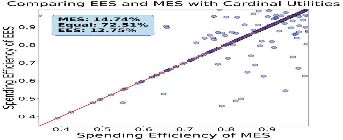
(a) Cardinal utilities.

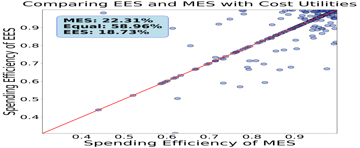
(b) Cost utilities.

Figure 2: Spending efficiency of MES and EES with add-one heuristic. Each point in the scatter point represents a Pabulib data set.

6.2 Heuristics for EES

Our primary motivation for introducing EES is that it admits a more sophisticated completion heuristic, namely, add-opt. Recall that, given a solution $(W,X)$ for $E(b)$, add-opt identifies the smallest value of $d$ such that $\mathit{EES}(E(b+nd))\neq(W,X)$. Crucially, this heuristic is based on reinterpreting the EES outcomes as outcomes that are stable in the sense of Definition˜4.1; it is not clear if MES outcomes can be interpreted in this way, and, as a consequence, we cannot use add-opt with MES. Indeed, for MES it is not known if the problem of finding the smallest budget increase that changes the outcome admits a polynomial-time (let alone a linear-time) algorithm.

When using EES with add-opt, we start by setting $b^{(1)}=b$, and compute $(W^{(1)},X^{(1)})=\mathit{EES}(E(b^{(1)}))$. Then in each iteration $i$ we compute $d^{(i)}$ by running add-opt on $E(b^{(i)})$ and $(W^{(i)},X^{(i)})$, and set $b^{(i+1)}=b^{(i)}+n\cdot d^{(i)}$, $(W^{(i+1)},X^{(i+1)})=\mathit{EES}(E(b^{(i+1)}))$. Just like with add-one, we repeat this procedure until the actual budget is exhausted or the next budget increment results in overspending. We also consider a complete version of this method EES + add-opt (C), where we increase the budget using add-opt until all projects are selected, i.e., $W^{(i)}=P$; then, among the outcomes $W^{(1)},\dots,W^{(i)}$ we select one that has the highest spending efficiency among all outcomes that are feasible for the original election $E(b)$. We define a complete version of MES with add-one (denoted by MES+add-one (C)) in a similar way.

Further, leveraging add-opt, we define a new completion method for EES, which we call add-opt-skip. This method modifies the add-opt heuristic in two key ways. First, given an outcome of EES, we invoke GreedyProjectChange (Algorithm˜5) only for projects not currently included in the outcome. Second, this process is repeated until all projects are considered for inclusion at least once. It then returns the feasible outcome with the highest spending efficiency found.

We evaluate all completion methods based on two criteria. The first is spending efficiency (as defined in Section˜6.1). The second is the number of calls to the computationally expensive base method (EES or MES) required by each completion method. All experiments are run under two assumptions: (1) cardinal utilities and (2) cost utilities.

Findings

Our results are summarized in Tables 1 and 2, and in Figure˜3(b). In both tables, the first three columns refer to the number of iterations, and the last three columns refer to the spending efficiency.

For add-opt, the mean per-voter budget increment size across our dataset is $37.3$ units for cost utilities and $35$ for cardinal utilities. The median of these budget increments is $6.4$ for cost utilities and $4.6$ for cardinal utilities. These values are greater than $1$, which means that typically add-opt considers substantially fewer budgets than add-one, while also guaranteeing the identification of a budget that maximizes the spending efficiency within the tested range.

Table 1: Comparison results: cardinal utilities.

Method	Avg	Med	Std	Avg	Med	Std
	Ex.	Ex.	Ex.	Eff.	Eff.	Eff.
MES + add-one	535.4	393.0	433.0	0.855	0.890	0.124
MES + add-one (C)	2888.7	1996.0	3132.4	0.862	0.896	0.123
EES + add-opt	279.6	100.0	356.3	0.848	0.888	0.130
EES + add-opt (C)	625.8	237.0	794.9	0.854	0.892	0.131
EES + add-opt-skip	27.9	17.0	27.3	0.853	0.890	0.130
max	563.3	423.0	425.5	0.871	0.906	0.119

Table 2: Comparison results: cost utilities.

Method	Avg	Med	Std	Avg	Med	Std
	Ex.	Ex.	Ex.	Eff.	Eff.	Eff.
MES + add-one	465.6	346.0	431.4	0.900	0.944	0.110
MES + add-one (C)	2894.9	2033.0	3125.8	0.902	0.945	0.109
EES + add-opt	432.7	106.0	751.2	0.881	0.944	0.140
EES + add-opt (C)	1263.6	360.0	1812.9	0.882	0.945	0.140
EES + add-opt-skip	12.4	10.0	7.3	0.855	0.903	0.138
max	478.0	357.0	428.9	0.909	0.950	0.103

Interestingly, we observe that in some iterations add-opt returns a per-voter increase of less than $1$. This means that add-one may skip possible allocations, and thus is not guaranteed to find the budget that results in the most spending-efficient outcome, even if that budget lies within the tested range. Indeed, in our dataset we find over $10$ such instances, demonstrating that this is not only theoretically possible, but something that occurs in realistic PB elections. In contrast, using add-opt enables us to consider every distinct allocation within our tested range.

(a) EES vs. MES number of iterations

(b) EES vs. MES spending efficiency

Figure 3: max is the result of running MES + add-one and EES + add-opt-skip and taking the result with the higher spending efficiency.

These experiments highlight the advantages of add-opt-skip. Below are our key findings:

1. EES with add-opt-skip requires an order of magnitude fewer calls to the base method than MES with add-one:

   • For cardinal utilities, the average number of calls drops from 535 to just 28.

   • For cost utilities, the average number of calls decreases from 466 to only 12.

   • Despite this, EES with add-opt-skip provides comparable spending efficiency: $0.85$ for cardinal utilities (vs. $0.86$ for MES with add-one) and $0.86$ for cost utilities (vs. $0.9$ for MES with add-one).

2. EES with add-opt-skip often outperforms MES in spending efficiency:

   • In 85% of datasets, EES with add-opt-skip achieves spending efficiency that is at least as high as that of MES with add-one, with strictly higher efficiency in 16% of cases for cardinal utilities. For cost utilities, its spending efficiency is at least as high as that of MES with add-one on 55% of the datasets and strictly higher on 8% of the datasets.

3. High spending efficiency on non-monotone instances:

   • In some real-world instances such as the one in Figure˜1, the optimal virtual budget (in terms of spending efficiency) is larger than the smallest virtual budget that causes overspending. We identify $14$ such instances for cardinal utilities and $3$ for cost utilities. Heuristics that terminate as soon as overspending occurs perform poorly on such instances. add-opt-skip, on the other hand, is able to explore the space of virtual budgets in a more comprehensive fashion, avoiding these worst-case scenarios, and demonstrates on average 10% higher spending efficiency in these cases (see Figure˜4).

For add-opt, the observed benefits are less pronounced. While it reduces the number of calls to EES compared to add-one, one needs to execute Algorithm˜5 (which has a runtime comparable to that of EES) for every EES run, leading to minimal computational savings.

Recommendations

Our experimental results suggest that EES+add-opt-skip achieves comparable spending efficiency to MES+add-one while (1) using orders of magnitude fewer calls to EES and Algorithm˜5, and (2) avoiding worst-case scenarios, such as the one illustrated in Figure˜1. These advantages make EES+add-opt-skip particularly suitable for real-world use in cities, as well as in computational experiments on synthetic data, where many repetitions are necessary for statistical significance. Alternatively, one can explore a hybrid approach, which runs both MES+add-one and EES+add-opt-skip, as it incurs a negligible computational overhead relative to MES+add-one (see Figure˜3(b)).

7 Conclusions

The Method of Equal Shares is the state-of-the-art proportional algorithm for participatory budgeting, which, however, suffers from underspending As designing a better algorithm for participatory budgeting is challenging, we can mitigate the issue of underspending (while maintaining all beneficial properties of MES) by identifying a virtual budget for which MES spends the maximum possible fraction of the true budget. However, this problem appears to be hard, so in practice the arguably arbitrary and inefficient add-one heuristic is used.

Our work presents a systematic and computationally-efficient solution to this problem for EES, which is a simplification of MES. We propose the add-opt algorithm for uniform utilities, which solves the problem of finding the minimum per-voter budget increase for which either a different winning set is selected, or more voters pay for a project, as opposed to arbitrarily incrementing each voter’s budget by $1. Importantly, the running time of this algorithm is linear in the number of voters $n$, which tends to be large in practice. The add-opt algorithm inspires the add-opt-skip heuristic, which only considers not yet selected projects. This heuristic is extremely computationally efficient, and therefore can be run until all projects are selected. As a result, in practice EES with this heuristic utilizes a comparable proportion of the budget to MES with add-one, while avoiding severe underutilization in non-monotonic examples such as that of Figure˜1. Moreover, running EES with add-opt-skip in parallel to MES with add-one and taking the output with the higher spending efficiency offers an increase in utilization across approval and cost utilities, as well as avoids worst-case examples, as seen in Figure˜1, for the price of, on average, just $12$ and $28$ additional executions of EES (Figure˜3(a)).

Throughout this paper, we focus on budget utilization. However, a similar methodology could be applied to select amongst EES outcomes based on any desirable property. Any such process would benefit greatly from only having to consider a reduced number of budget increments, particularly in the realm of experimental work, where large numbers of instances may be required in order to have high statistical confidence in claimed results. The importance of such work becomes clear when one considers the real-world impact that even a single additional project can have on the lives of the voters, especially as participatory budgeting grows in size and scale. Further, while we show that the number of distinct outcomes as one varies the budget may be exponential in the instance size, the speed-up due to our efficient heuristic makes the identification of all outcomes feasible in practice.

Open Problems

We showed that for cost utilities the number of distinct outcome returned by EES for different budgets can be exponential in the size of the instance. For cardinal utilities, this question remains open: is the dependency exponential, or can it be bounded by a polynomial in the size of the instance? More generally, a challenging open problem is to pin down the complexity of directly finding a virtual budget for which EES (or MES) finds a feasible solution that spends the maximum fraction of the true budget. As a starting point, one may consider the problem of deciding whether there exists a virtual budget for which EES (or MES) spend exactly the entire true budget.

Appendix A Proofs Omitted from the Main Text

See 3.2

Proof.

Let $W$ be the outcome selected by Exact Equal Shares on instance $(N,P,(A_{i})_{i\in N},b,{\mathit{cost}})$. Let $S$ be a $T$-cohesive group for $T\subseteq P$. Let $Y\subseteq T$ be the set of projects in $Y$ paid for by less than $|S|$ voters (this includes being paid by no voters). If the set $Y$ is empty, we are done since every voter $i\in S$ has utility $u_{i}(W)$ for the outcome satisfying $u_{i}(W)\geq u(T)$. So suppose set $Y$ is non-empty. Let $y^{*}\in\operatorname*{arg\,max}_{y\in Y}\frac{u(y)}{{\mathit{cost}}(y)}$. There must be some voter $i\in S$ such that the budget $z_{i}$ not being used to pay for projects at bang per buck at least $\frac{u(y^{*})|S|}{{\mathit{cost}}(y^{*})}$ (this includes leftover budget) satisfies the inequality $z_{i}<\frac{{\mathit{cost}}(y^{*})}{|S|}$, as otherwise the voters in $S$ could jointly pay for a project from set $Y$. Now voter $i$ may spend some of her money on projects $T\setminus Y$, each such project $P$ it pays for at most $\frac{{\mathit{cost}}(p)}{|S|}$. So on projects in $W\setminus T$ with bang per back at least $\frac{u(y^{*})|S|}{{\mathit{cost}}(y^{*})}$, $i$ spends at least $\frac{b}{n}-\sum_{p\in T\setminus Y}\frac{{\mathit{cost}}(p)}{|S|}-z_{i}$. So her utility for the set $W\setminus T$ can be lower bounded as follows

$$u_{i}(W\setminus T) \geq\frac{u(y^{*})|S|}{{\mathit{cost}}(y^{*})}\left(\frac{b}{N}-\sum_{p\in T\setminus Y}\frac{{\mathit{cost}}(p)}{|S|}-z_{i}\right)$$

$$\geq\frac{u(y^{*})}{{\mathit{cost}}(y*)}\cdot\left({\mathit{cost}}(T)-\sum_{p\in T\setminus Y}{\mathit{cost}}(p)\right)-\frac{|S|z_{i}\cdot u(y^{*})}{{\mathit{cost}}(y*)}$$

$$>\frac{u(y^{*})}{{\mathit{cost}}(y*)}\cdot{\mathit{cost}}(Y)-|S|\frac{{\mathit{cost}}(y^{*})}{|S|}\frac{u(y^{*})}{{\mathit{cost}}(y*)}$$

$$\geq\sum_{y\in Y}{\mathit{cost}}(y)\frac{u(y^{*})}{{\mathit{cost}}(y^{*})}-u(y^{*})$$

$$\geq\sum_{y\in Y}{\mathit{cost}}(y)\frac{u(y)}{{\mathit{cost}}(y)}-u(y^{*})$$ (2)

$$=\sum_{y\in Y}u(y)-u(y^{*}),$$

where the line 2 follows since $y^{*}$ gives the largest value of $\frac{u(y)}{{\mathit{cost}}(y)}$ among all projects $y\in Y$. Overall, voter $i$ has utility at least

$$u_{i}(W\setminus T)+u_{i}(T\setminus Y)>$$

$$u_{i}(Y)+u_{i}(T\setminus Y)-u(y^{*})=u(T)-u(y^{*})$$

for projects in $W$ that are paid for by at least $|S|$ people, implying that after including $y^{*}$ we get

$$u(W\cup\{y^{*}\})\geq u(W\setminus T)+u(T\setminus Y)+u(y^{*})>u(T),$$

as desired. ∎

See 5.1

Proof.

Let $v\in V\setminus N_{p}(X)$ has $r_{v}\geq\frac{{\mathit{cost}}(p)}{|V|}$ or $(\frac{{\mathit{cost}}(p)}{|V|},p)<_{\textit{lex}}c_{v}$. In the latter case, the voter spends at least $\frac{{\mathit{cost}}(p)}{|V|}$ on a less preferred project $p^{\prime}$. So the sum of her leftover budget and the budget she spends on less preferred projects is at least $\frac{{\mathit{cost}}(p)}{|V|}$, as desired.

For the other direction of the claim, suppose now voter $v$ has $t_{v}\geq\frac{{\mathit{cost}}(p)}{|V|}$ where $t_{v}$ is the combined total of $r_{v}$ and the money spent on projects $p^{\prime}$ in $\{p^{\prime}\mid(\textit{BpB}(p^{\prime}),p^{\prime})<_{t}(\frac{u(p)t}{cost(p)},p)\}$. If the latter set is empty, then $r_{v}\geq\frac{{\mathit{cost}}(p)}{|V|}$. If it is non-empty, then such a project $p^{\prime}$ has

$$BpB(p^{\prime})\leq\frac{u(p)|V|}{{\mathit{cost}}(p)}\iff\frac{u(p^{\prime})|N_{p^{\prime}}(X)|}{{\mathit{cost}}(p^{\prime})}\leq\frac{u(p)|V|}{{\mathit{cost}}(p)}\iff$$

$$\frac{|N_{p^{\prime}}(X)|}{{\mathit{cost}}(p^{\prime})}\leq\frac{|V|}{{\mathit{cost}}(p)}\iff\frac{{\mathit{cost}}(p)}{|V|}\leq\frac{{\mathit{cost}}(p)}{|N_{p^{\prime}}(X)|}.$$

So it follows that $(\frac{cost(p)}{|V|},p)<_{\textit{lex}}(\frac{{\mathit{cost}}(p)}{|N_{p^{\prime}}(X)|},p^{\prime})$ implying in particular that $(\frac{cost(p)}{|V|},p)<_{\textit{lex}}c_{v}$. So $r_{v}\geq\frac{cost(p)}{|V|}$ or $(\frac{cost(p)}{|V|},p)<_{\textit{lex}}c_{v}$ hold, implying that $v$ is willing to contribute $\frac{{\mathit{cost}}(p)}{|V|}$ to $p$.∎

See 4.2

Proof.

This follows directly from Lemma˜5.1 and Proposition˜5.2 (proved below). ∎

See 5.2

Proof.

Let $E$ be an election and let $(W,X)=EES(E)$. We can trivially modify EES to return the selected projects in $W$ in the order they were selected, i.e. in order of non-increasing bang per buck (with lexicographic tie-breaking). We will denote this sequence as $p_{1},p_{2},\ldots,p_{w}$ where $w=|W|$. Suppose for the sake of contradiction that $(W,X)$ is unstable, as certified by a pair $(p,V)$. Then for every $v\in V$ we have $r_{i}(v)\geq\nicefrac{{{\mathit{cost}}(p)}}{{|V|}}$ where $i$ is the smallest index for which $(\textit{BpB}(p_{i}),p_{i})<_{t}(\frac{u(p)|V|}{{\mathit{cost}}(p)},p)$. Since $(W,X)$ is unstable, we have that $i$ is well-defined. Now consider the project selected in the $i$th iteration of EES in which $p_{i}$ is selected. By the definition of EES the project $p$ is affordable by voters $V$ in this round since by the choice of $i$, $r_{i}(v)\geq\nicefrac{{{\mathit{cost}}(p)}}{{|V|}}$. Furthermore, since $(\textit{BpB}(p_{i}),p_{i})<_{t}(\frac{u(p)|V|}{{\mathit{cost}}(p)},p)$ holds, project $p$ has higher priority than $p_{i}$, and so would be selected by EES instead. This contradicts that EES returns $(W,X)$ and the project ordering projects $p_{1},\ldots,p_{w}$. We conclude that $(W,X)$ is stable. ∎

We now show how to compute $L_{1},\ldots,L_{w}$ used in Algorithm˜4 and computed in Algorithm˜5 given $L_{w+1}$ and $p_{1},\ldots,p_{w}$ using dynamic programming.

Lemma A.1.

Suppose we have $W$ given in order $p_{1},\ldots,p_{w}$ such that $(\textit{BpB}(p_{i}),p_{i})>_{\textit{t}}(\textit{BpB}(p_{i+1}),p_{i+1})$ as well as $L_{w+1}$. Then we can compute $L_{1},\ldots,L_{w}$ in time $O(mn)$.

Proof.

$L_{i}$ will contain the values $r_{i}(v)$ sorted in non-decreasing order. We note that either a voter contributes to project $p_{i}$ or she does not, and in the former case, every such voter contributes an equal amount by the definition of exact equal shares. So to obtain $L_{i}$ from $L_{i+1}$ it suffices to merge the sorted lists $L_{i+1}[N_{p_{i}}(X)]+\frac{{\mathit{cost}}(p_{i})}{|N_{p_{i}}(X)|}$ (voters who pay for $p_{i}$) and $L_{i+1}[O_{p_{i}}(X)]$ (voters who do not pay for $p_{i}$) in time $O(n)$. Since we create $w=O(m)$ lists this way, the overall runtime is $O(mn)$. ∎

See 5.6

Proof.

By Lemma˜A.1 lists $L_{1},\ldots L_{w}$ can be computed in time $O(mn)$ from the ordering $p_{1},\ldots,p_{w}$ and $L_{w+1}$. For the remainder of Algorithm˜5, we execute Algorithm˜4 $m$ times which by Lemma˜5.5 can be implemented in time $O(m+n)$. However, when calling GreedyProjectChange in Algorithm˜5, we partially copy the lists $L_{1},\ldots,L_{w+1}$ to obtain the sublists $L_{1}(O_{p}(x))\ldots L_{w+1}(O_{p}(X))$ which takes time $O(mn)$, resulting in an overall runtime of $O(m^{2}n)$. This completes the proof. ∎

See 5.7

Proof.

The proof proceeds in analogy to the proof of Theorem˜4.9 with minor differences. Let $(W^{*},X^{*})=EES(E(b+nd^{*}))$. Since $(W,X)\neq(W^{*},X^{*})$ we show that there exists $(p,V_{p})$ that certifies the instability of $(W,X)$ for budget $b^{*}$, i.e. after an increase of $\frac{b^{*}-b}{n}$ per voter from budget $b$; indeed, there exists a first iteration, say iteration $q$, in which EES selects a project $p$ paid for by voters $V_{p}$ for $E(b+nd^{*})$, such that in the $q$th iteration for $E(b)$ for budget $b$ the same does not happen (more precisely, the algorithm may terminate before iteration $q$ or it may not select $p$ in iteration $q$, or it may be pair for by a different set of voters). For budget $b$, either $p$ is never selected or it is eventually selected. In the first case this means that for budget $b^{*}$ at the end of iteration $q-1$, every voter $v\in V_{p}$ has $r_{i}(v)\geq\frac{{\mathit{cost}}(p)}{|V_{p}|}$ for some $i$ with $BpB(p_{i}),p_{i})<_{t}(\frac{u(p)|V_{p}|}{{\mathit{cost}}(p)},p)$ which by Lemma˜5.3 implies that $(V_{p},p)$ certifies the instability of $(W,X)$ for budget $b^{*}$, as claimed. If instead $p$ is (eventually) selected for budget $b$, it will be paid for by a strict subset of the voters $V_{p}$; indeed if there was be a voter $v\notin V_{p}$ paying for $p$, then this voter would also pay for $p$ in EES run on $E(b^{*})$. Clearly $p$ cannot be paid for by all of $V_{p}$, as then EES would select $p$ paid for by $V_{p}$ in iteration $q$ for both elections $E$ and $E^{*}$, contrary to our assumption. However, as before, every voter $v\in V_{p}$ has $r_{i}(v)\geq\frac{{\mathit{cost}}(p)}{|V_{p}|}$ for some $i$ with $BpB(p_{i}),p_{i})<_{t}(\frac{u(p)|V_{p}|}{{\mathit{cost}}(p)},p)$ which by Lemma˜5.3 implies that $(V_{p},p)$ certifies the instability of $(W,X)$ for budget $b^{*}$, as claimed. So since an increase of $\frac{b^{*}-b}{n}$ per voter results in $p$ certifying the instability of $E$, by Theorem˜4.6, Algorithm˜2 for $p$ will return an amount $d\leq\frac{b^{*}-b}{n}$, so that the output $b^{\prime}$ of Algorithm˜3 is at most $b^{*}$. Furthermore, for $b^{\prime}=b+dn$ where $d$ is computed by Algorithm˜3, there exists $(p^{\prime},V_{p}^{\prime})$ that certifies instability of $(W,X)$. Since EES returns stable outcomes, this implies that for budget $b^{\prime}$, EES does not return $(W,X)$ i.e. $EES(E(b^{\prime}))\neq(W,X)$ and so by our definition of $b^{*}$ it follows that $b^{*}\leq b^{\prime}$. This concludes the proof. ∎

Appendix B Further Experimental Results

Efficiency on Non-Monotonic Instances

Figure˜4 examines cases where the optimal spending efficiency is achieved after the point where the true budget is first overspent.

Figure 4: Graph showing executions and spending efficiency for identified cases where the optimal virtual budget occurs after the point at which the true budget is first overspent. In these cases, EES with add-opt-skip achieves much higher spending efficiency than MES with add-one, increasing from an average of 78% to 86% for the 3 identified instances with cost utilities and from 78% to 90% for the 14 identified instances with cardinal utilities.

Figure 5: Spending efficiency of EES with add-opt-skip vs. MES with add-one: cardinal utilities.

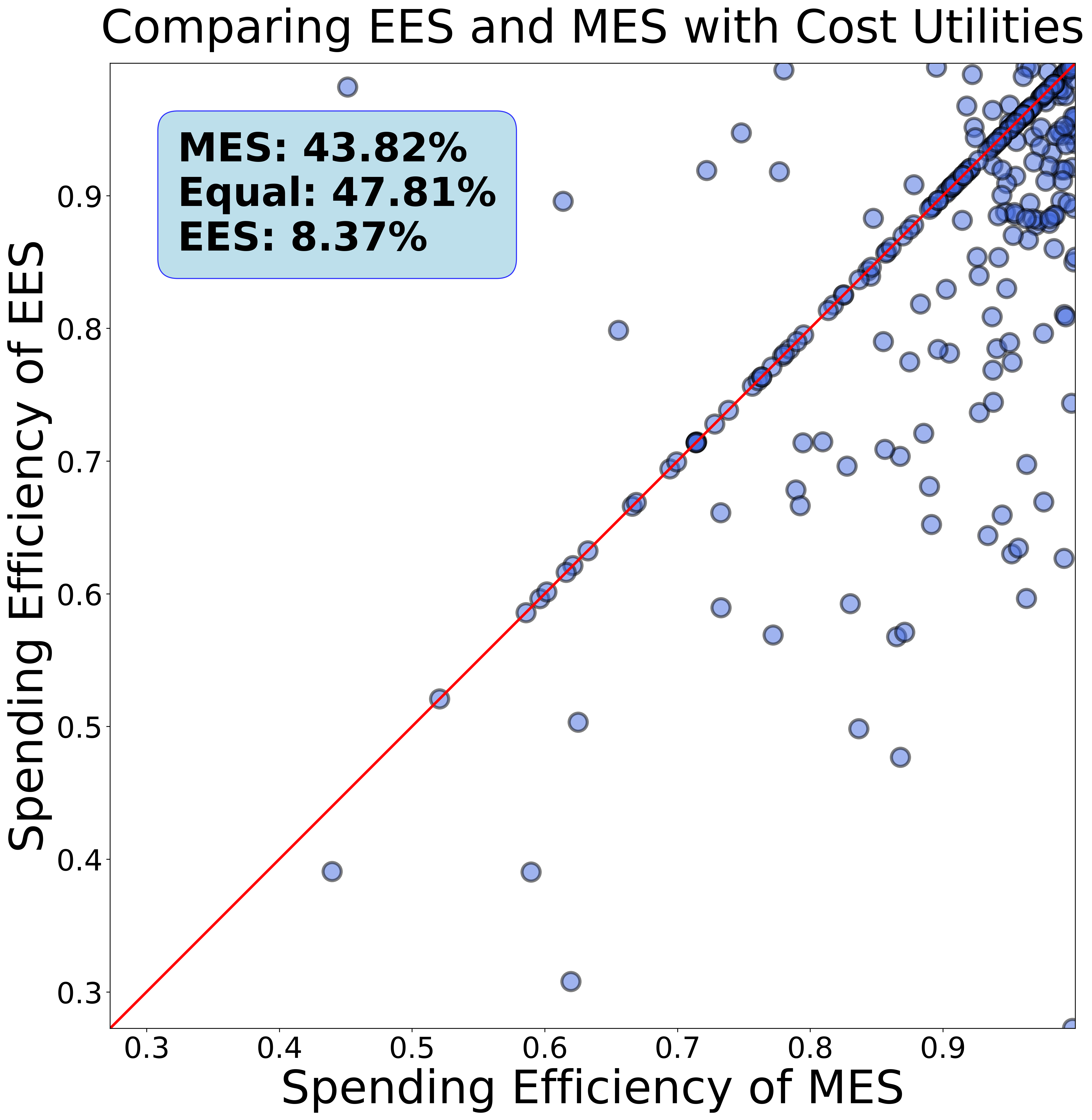
Figure 6: Spending efficiency of EES with add-opt-skip vs. MES with add-one: cost utilities.

Dataset Analysis

Figure˜7 presents key characteristics of our dataset, including distributions of voters, projects, and budgets.

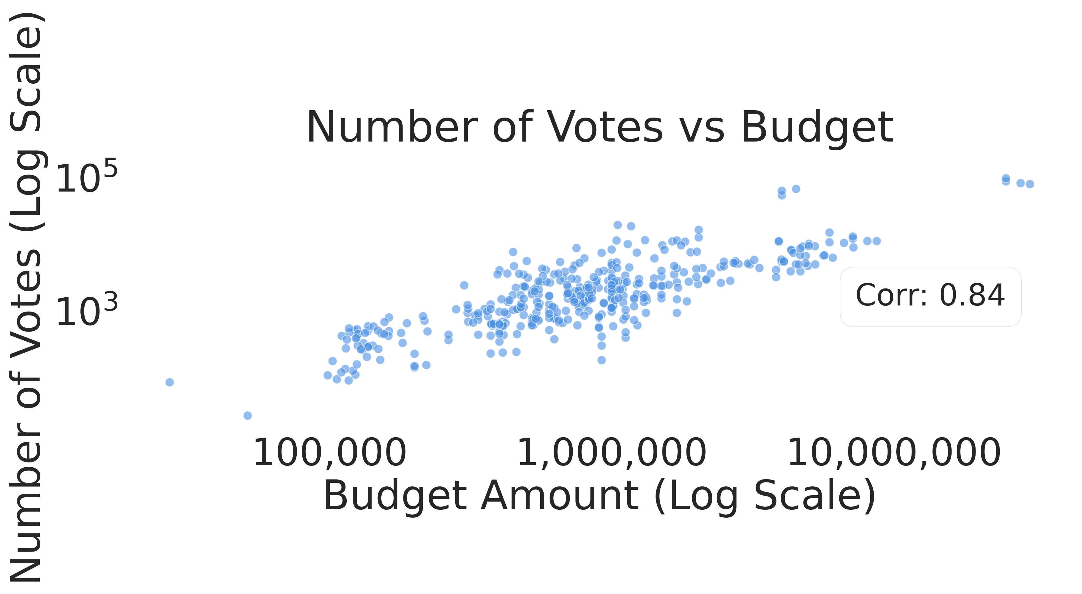
(a) Number of voters versus budget amount in the selected Pabulib instances.

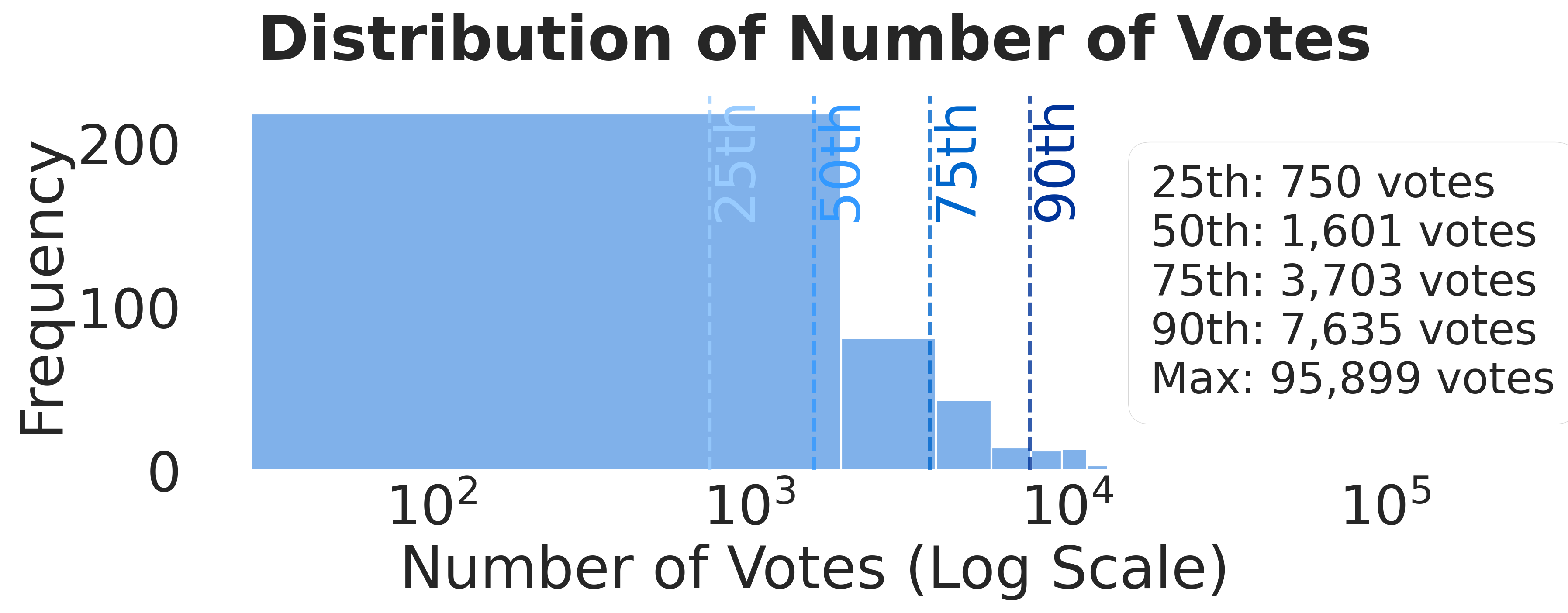
(b) Histogram of the number of voters across all selected Pabulib instances.

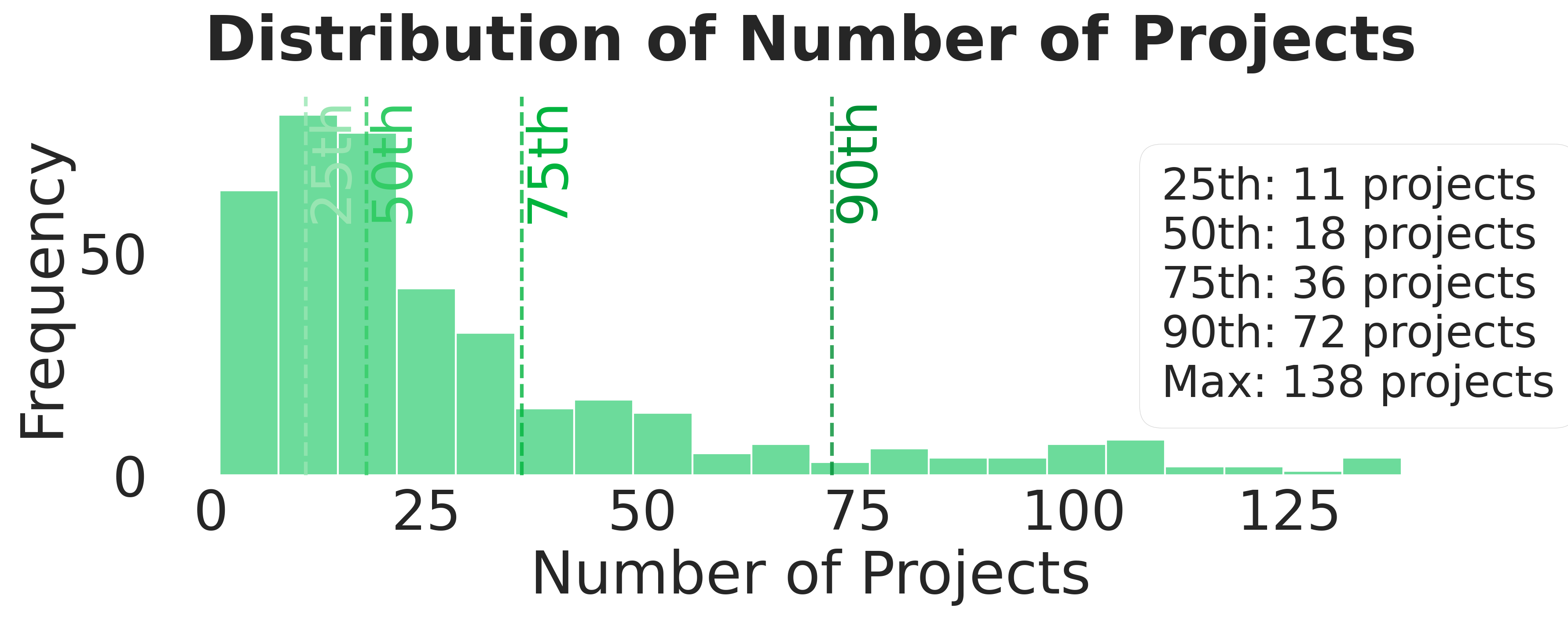
(c) Histogram of the number of projects across all selected Pabulib instances.

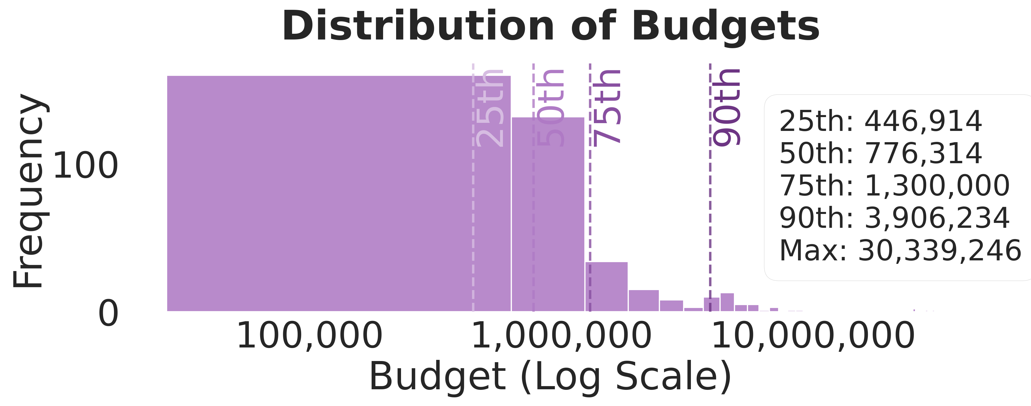
(d) Histogram of the budget size across all selected Pabulib instances.

Figure 7: Dataset characteristics showing the distribution of voters, projects, and budgets across all analyzed Pabulib instances.

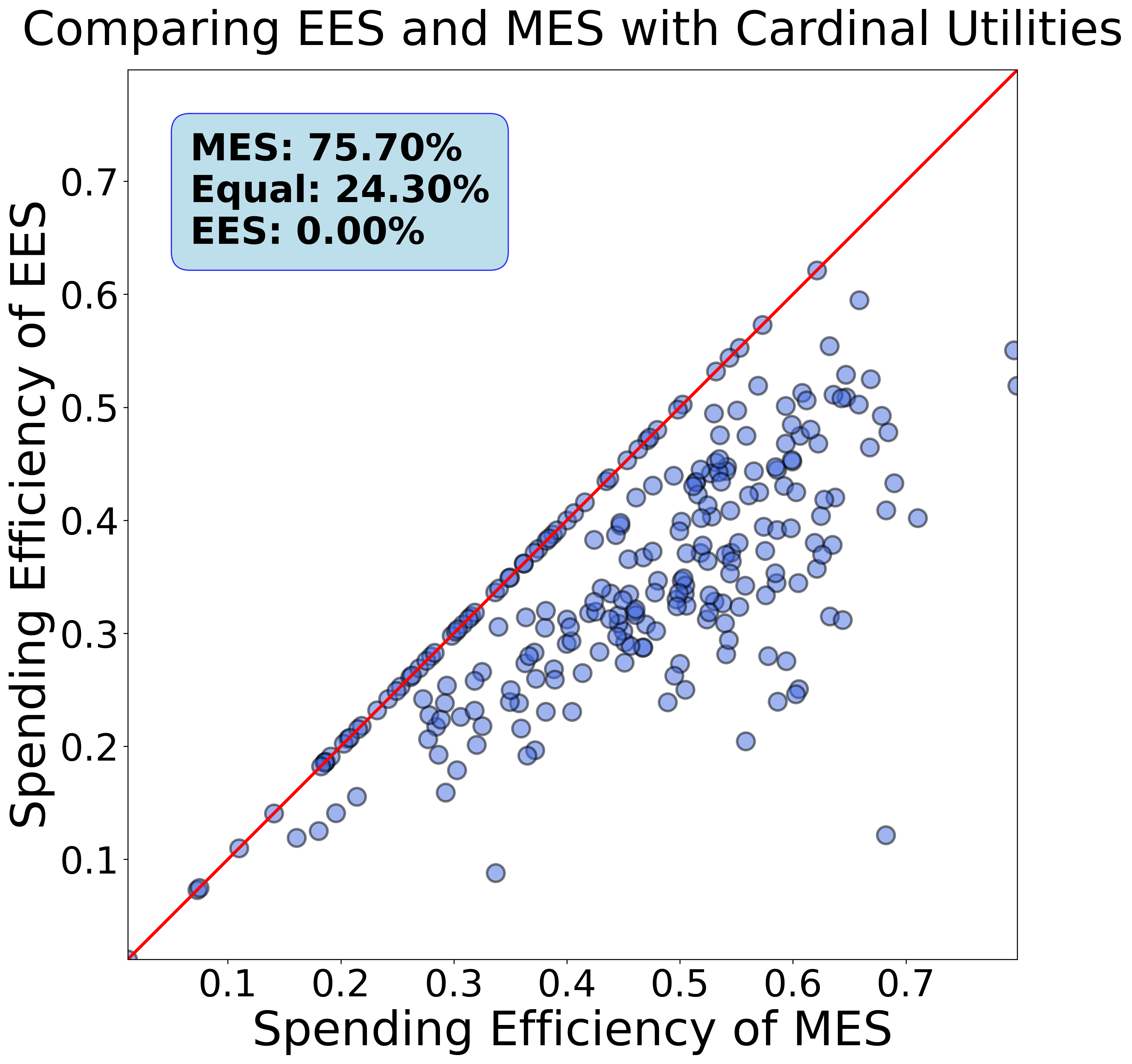
Figure 8: A comparison of the spending efficiency of MES vs. EES without a completion method: cardinal utilities.

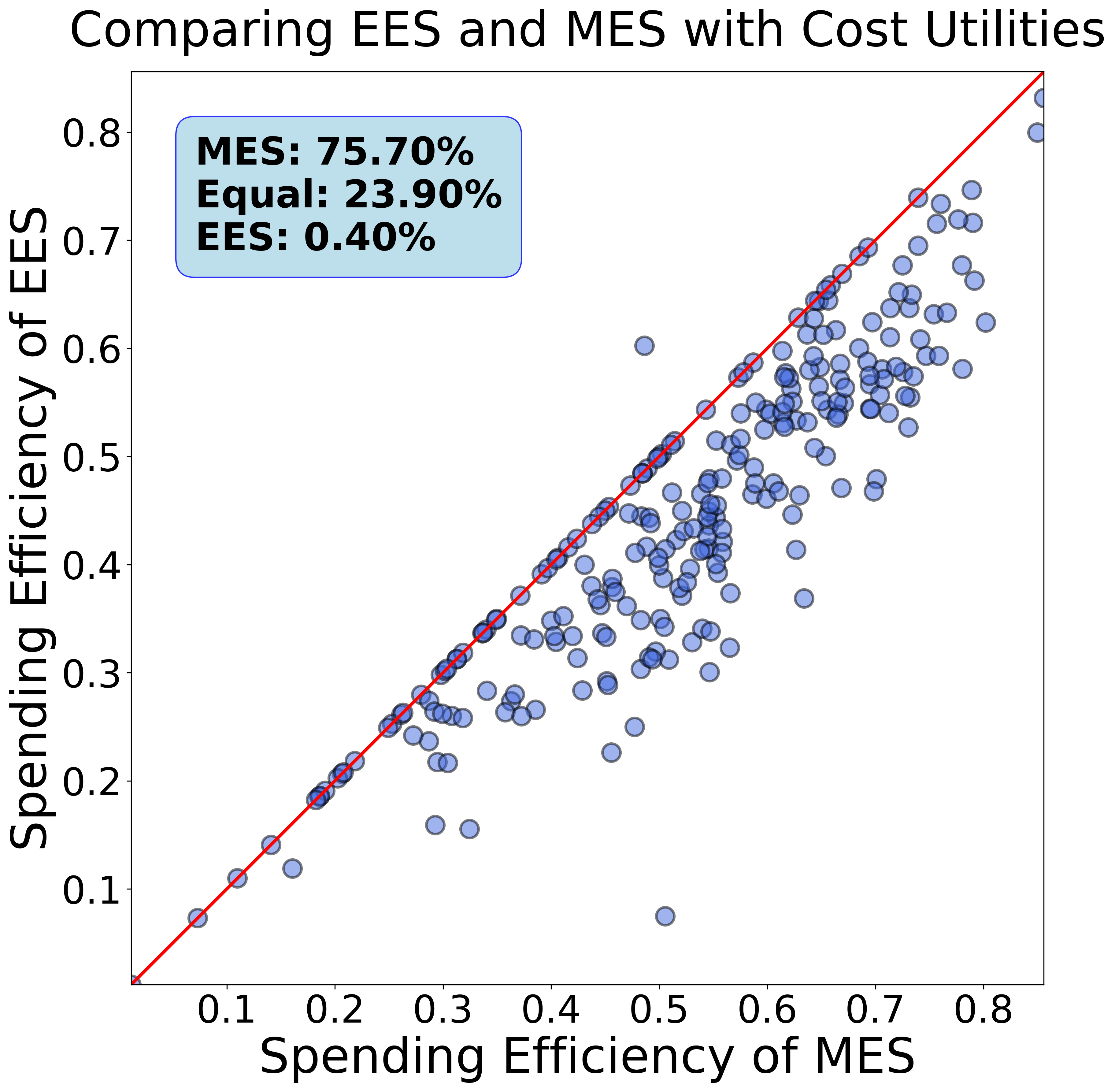
Figure 9: A comparison of the spending efficiency of MES vs. EES without a completion method: cost utilities.

Case Study: Stare Implementation

Figure˜10 examines a specific implementation from Stare, Poland, demonstrating how project selection changes with budget allocation.

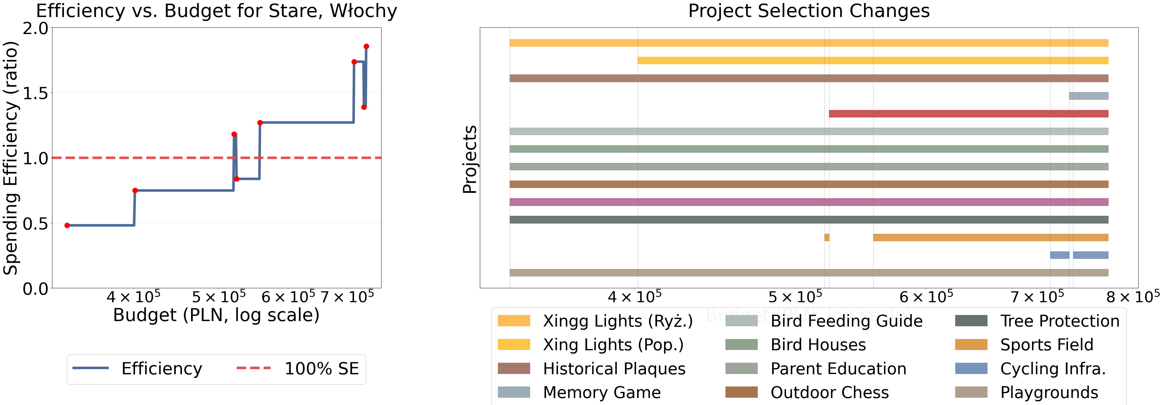
Figure 10: Graph showing which projects are implemented for a given budget for an instance from Stare, Poland using add-one until all projects are selected for the first time. The left shows the spending efficiency for the given virtual budget, the right shows the specific projects implemented for that budget.

References

- Aziz et al. [2017] H. Aziz, M. Brill, V. Conitzer, E. Elkind, R. Freeman, and T. Walsh. Justified representation in approval-based committee voting. Social Choice and Welfare, 48(2):461–485, 2017.
- Aziz et al. [2018] H. Aziz, E. Elkind, S. Huang, M. Lackner, L. Sánchez-Fernández, and P. Skowron. On the complexity of extended and proportional justified representation. In AAAI’18, 2018.
- Chohan [2017] U. W. Chohan. The decentralized autonomous organization and governance issues. In Decentralized Autonomous Organizations, pages 139–149. Routledge, 2017.
- De Vries et al. [2022] M. S. De Vries, J. Nemec, and D. Špaček. International trends in participatory budgeting. Cham: Palgrave Macmillan, 2022.
- Faliszewski et al. [2023] P. Faliszewski, J. Flis, D. Peters, G. Pierczyński, P. Skowron, D. Stolicki, S. Szufa, and N. Talmon. Participatory budgeting: Data, tools, and analysis, 2023. URL https://arxiv.org/abs/2305.11035.
- Jain and Mahdian [2007] K. Jain and M. Mahdian. Cost sharing. In Algorithmic game theory, chapter 15, pages 385–410. Cambridge University Press, 2007.
- Janson [2016] S. Janson. Phragmén’s and Thiele’s election methods. arXiv preprint arXiv:1611.08826, 2016.