[orcid=0000-0002-7235-7805] \cormark[1] \cortext[cor1]Corresponding authors. \creditData curation, Formal analysis, Funding acquisition, Investigation, Visualization, Writing - Original Draft, Writing – review & editing
[orcid=0000-0002-0709-042X] \creditConceptualization, Supervision, Writing – review & editing
[orcid=0000-0002-6039-780X] \cormark[1] \creditConceptualization, Formal analysis, Funding acquisition, Investigation, Methodology, Project administration, Supervision, Validation, Writing – review & editing
Surface magnetoelectric driven spin dynamics in metallic antiferromagnets
Abstract
Although magnetoelectric effects in metals are usually neglected, assuming that applied electric fields are screened by free charge carriers, the skin depth, defining the penetration depth of the fields, is non-zero and for THz electric fields typically reaches 400 nm. Hence, if the thickness of an antiferromagnetic film is of the order of tens of nm, electric field induced effects cannot be neglected. Here, we theoretically study the THz electric field induced spin dynamics in the metallic antiferromagnets and , whose spin arrangements allow them to exhibit a linear magnetoelectric effect. We shown that the THz magnetoelectric torque in metallic antiferromagnets is proportional to the time derivative of the THz electric field induced polarization. Our calculations reveal that the magnetoelectric driven spin dynamics is indeed not negligible and can fairly explain the previously published experimental results on antiferromagnetic dynamics excited by the THz pump pulses in at the corresponding magnetoelectric susceptibility value without involving other mechanisms. This value is about one order of magnitude smaller than that known for collinear and rare-earth-free antiferromagnets such as . For such a value of magnetoelectric response, it appears that the THz electric fields of realistic strengths of about 1 MV/cm are sufficient in order to achieve spin dynamics with the amplitudes sufficiently strong enough for switching of the antiferromagnetic Néel vector between the stable ground states. Thus, we contend that the experimental studies of the coherent dynamics of the antiferromagnetic vector driven by the THz pulses in magnetoelectric metal films necessitate a careful consideration of the linear magnetoelectric effect.
keywords:
Magnetoelectric effect \sepMetallic antiferromagnets \sepSpin dynamics \sepSpin switching1 Introduction
Antiferromagnets form the largest, least explored, but probably the most intriguing class of magnetic materials promising to revolutionize spintronic technologies. In particular, it is believed that the use of antiferromagnets can push the rates of processing magnetically stored data to the THz domain [1, 2, 3, 4, 5]. In the simplest case, an antiferromagnet is described as two antiferromagnetically coupled and completely equivalent ferromagnetic sublattices, with magnetizations and , respectively. The antiferromagnetic order parameter in this case is the antiferromagnetic Néel vector . Finding the mechanisms allowing to control spins in antiferromagnets has been as a challenge from the discovery of antiferromagnetism because neither electric nor magnetic field seems to couple to the order parameter, at least in the simplest model of antiferromagnet, a and .
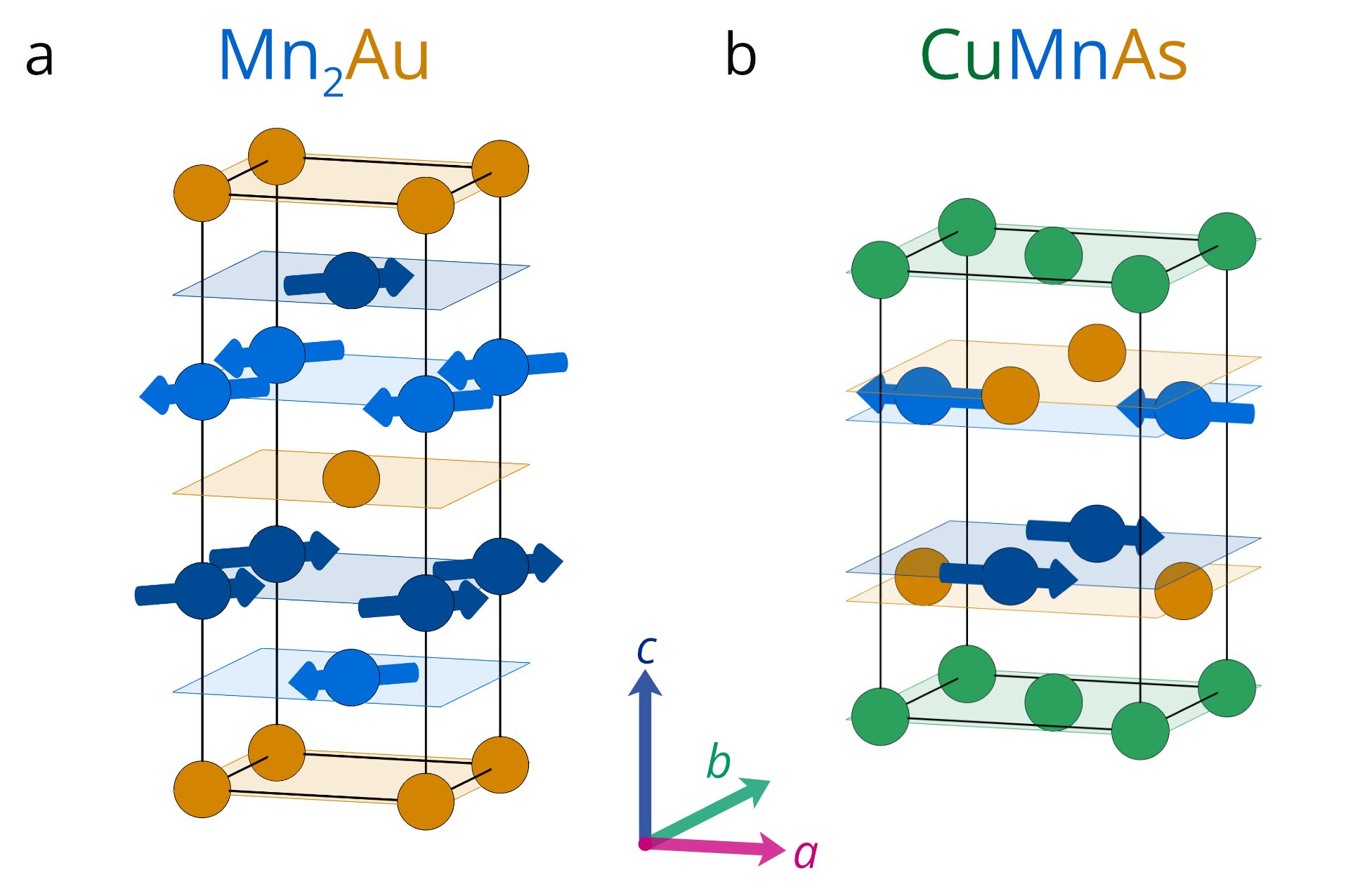
There are two prototypical antiferromagnetic metallic spintronic materials, Mn2Au and CuMnAs, in which the breaking of the inversion and time-reversal symmetry, while their combination is preserved and connects two oppositely aligned Mn magnetic sublattices, leading to a linear magnetoelectric effect [6, 7] and allowing to couple the electric field to the antiferromagnetic order parameter as in the case of insulating [8, 9, 10]. In metals and semimetals, the free carriers screen an externally applied electric field at depths greater than the skin depth, and the linear magnetoelectric effect is therefore negligible. On the other hand, materials with the symmetry that allows magnetoelectric effect may also possess magnetogalvanic effects, where the antiferromagnetic Néel vector is coupled to an electrical current [11, 12]. Switching of the antiferromagnetic Néel vector between allowed ground states under the influence of charge and spin-polarized currents has been predicted and experimentally demonstrated in the metals Mn2Au and CuMnAs via the Néel spin-orbit torque [13, 14, 15], as well as quench switching [16, 17] mechanisms. However, in thin films of Mn2Au and CuMnAs with a thickness less than the skin depth, roughly estimated at about 400 nm for the 1 THz radiation [18], the applied THz electric field penetrates into the material, which should also result in a magnetoelectric response.
Here, we present a theoretical study of the THz driven spin dynamics in the metallic magnetoelectric antiferromagnets Mn2Au and CuMnAs films with a thickness less than the skin depth. Employing the Lagrangian approach, we derive differential equations that take into account the linear magnetoelectric effect and describe the coherent dynamics of the antiferromagnetic Néel vector near the ground state under the action of the electric and magnetic fields of THz pulses. We show that our model, taking into account only the linear magnetoelectric effect of the corresponding strength, is able to describe the results of the THz experiment given in Ref. [19] without involving other mechanisms of the spin dynamics excitations. Thus, we have shown that the experimental studies of antiferromagnetic Néel vector switching by the strong picosecond pulses of THz electric fields in these spintronic materials require the consideration of the magnetoelectric effect.
2 Magnetoelectric antiferromagnets
Mn2Au and CuMnAs (orthorhombic in the bulk form and tetragonal in the thin film grown on GaAs or GaP [20]) with tetragonal crystal structures have the nonsymmorphic space groups (#139, ) [21] and (#129, ) [20] and four formula units per unit cell , respectively. The lattice parameters at room temperature are Å and Å for Mn2Au [21] and Å and Å for CuMnAs [22]. At room temperature both Mn2Au ( [21] that exceeds the temperature about K at which the compound becomes structurally unstable [23]) and CuMnAs ( K [22]) provide a collinear antiferromagnetic structure with ferromagnetic layers in the plane antiferromagnetically aligned along the axis [21, 22]. For Mn2Au in-plane diagonals are easy axes of magnetic anisotropy () [21, 24] while for CuMnAs the and are easy axes () [22, 25]. Besides, the energy barrier between the and easy axes in both compounds is small, and has a value of about 1 V per formula unit [22, 14]. Thus, four types of different antiferromagnetic domains are expected in these materials [26]. The crystal structure and magnetic ordering of Mn2Au and CuMnAs are shown in Fig. 1. Further we assume that , , and .
3 Magnetoelectric model
We have developed a model of magnetoelectric-driven spin dynamics near the ground state in a metallic antiferromagnet Mn2Au only because the results for the CuMnAs will be qualitatively similar. The magnetic moment of ions is of the same value , so it is convenient to use the two-sublattice approximation with two opposite sublattice magnetizations and . Then we define the net magnetization vector and antiferromagnetic vector . We use the spherical coordinate system with polar and azimuthal angles, where the sublattice magnetization vectors are . Then, and are parameterized as follows [27, 28, 29]
| (1) |
where small canting angles and are introduced. We expand the net magnetization and antiferromagnetic vector Cartesian components in series with respect to the small canting angles and . The resulting expressions are
| (2) |
The magnetic moments of the ions are aligned in the plane of Mn2Au. The energy of the easy-plane magnetic anisotropy, taking into account Eq. (2), has the form
| (3) |
where are the easy-plane magnetic anisotropy parameters. To find the ground state we minimize with respect to and angles by solving the equations
| (4) |
with the assumption that , , and and the following conditions
| (5) |
Then the ground state is defined by the angles , and , .
Near the ground state the angles can be expressed as and , where and . Then, taking into account the following relations
| (6) |
we can represent vector components and [Eqs. (2)] in the following form
| (7) |
Thus, the anisotropy energy (3) in the vicinity of the magnetic ground state up to a constant term can be represented as
| (8) |
where the used parameters are , , .
The kinetic energy of the spin system in a double-sublattice antiferromagnet per one magnetic ion can be determined through the Berry phase gauge [30, 29] in the first order in and as
| (9) |
where is the spin for magnetic ions and is the gyromagnetic ratio.
The exchange energy of the magnetic system in a double-sublattice antiferromagnet in the second order of and up to a constant term can be represented as
| (10) |
where is the exchange interaction constant between neighboring spins of ions.
The interaction of the spin system with the external magnetic field applied in the plane is described by the Zeeman term, which according to Eqs. (2) and (7) has the following form
| (11) |
According to the symmetry, the magnetoelectric energy in CuMnAs and Mn2Au has the following form
| (12) |
where are the dimensionless magnetoelectric parameters. For simplicity, we assume that the polarization is induced by the electric field applied in the plane. Note that since spin dynamics will be considered, the expression for [Eq. (12)] is given for polarization , which is a dynamical variable, and not for the electric field , which is an external influence in this case [8]. Then, taking into account Eq. (7) and neglecting small angles above the second order, Eq. (12) near the ground state has the form
| (13) |
To reveal the spin dynamics induced by the electric and magnetic fields we construct a Lagrangian general expressions for the exchange (10), anisotropy (3), magnetoelectric (13) energies and expression for the kinetic energy close to Eq. (9)
| (14) |
The Rayleigh dissipation function is [7]
| (15) |
where is the Gilbert damping constant. Note that all terms in Eq. (14) are considered for a single molecule units. Then we substitute the Lagrangian (14) and Rayleigh dissipation function (15) into the Euler-Lagrange equations
| (16) |
where for – are order parameters , , , and , respectively. As a result, we obtain a system of four differential equations describing the spin dynamics of the magnetoelectric antiferromagnet induced by the electric and magnetic fields
| (17) |
where the used parameters are , , , and ps is the magnon damping time from Ref. [19], that we introduced into the system of differential equations.
4 THz driven spin dynamics
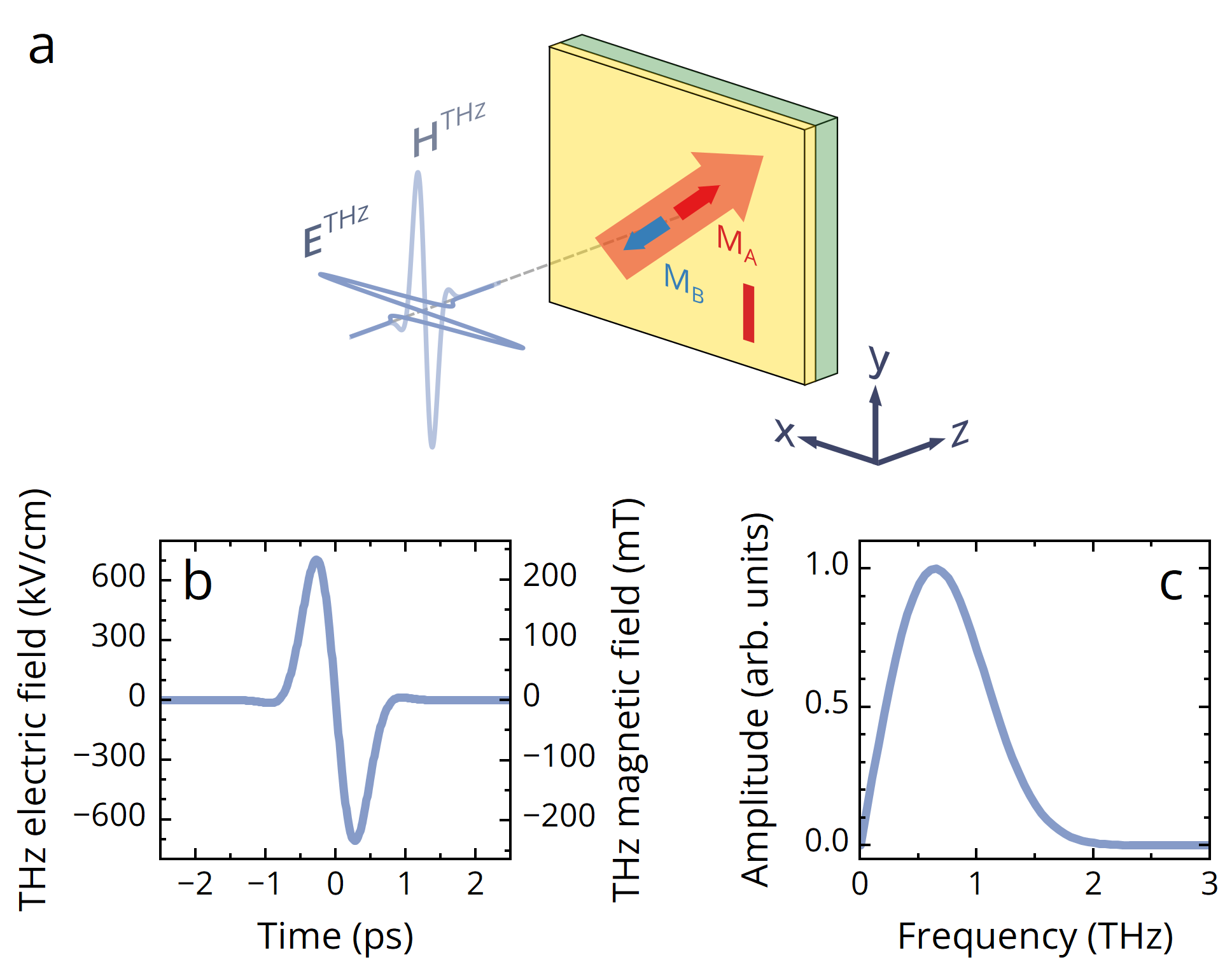
The THz electric and magnetic field pulses are effective stimuli for the excitation of spin dynamics in antiferromagnets [1, 31, 32, 33]. To simulate the THz driven spin dynamics experiment (see Fig. 2a), we solve the Eq. (17) with a near single-cycle THz pulse given by the Gaussian function for the THz electric field
| (20) |
where is the peak electric field strength, and determine the THz pulse duration and frequency, respectively. The THz magnetic field is related to the THz electric field as in Gaussian units. For the THz pulse propagating along the axis the electric and magnetic field strength vectors are defined as and , where is the polarization angle with respect to the axis. Note that and are perpendicular to each other. The THz pulse parameters from Eq. (20) were taken close to the experimental one with peak electric field strength 760 kV/cm and corresponding magnetic field 250 mT, with a pulse duration about 2 ps and maximum on the spectra at the 0.6 THz as shown in Fig. 2b and 2c. The emerging spin response can be detected experimentally using femtosecond magneto-optic probes [3].
It is well known that the tangential component of the strength of the THz electric field on the surface with infinite conductivity is zero [34]. In the surface with finite but good conductivity and thickness larger than the spin depth, the tangential component of obeys the Leontovich boundary condition , where is the effective surface impedance and is the magnetic permeability of free space [34]. In our case, we assume that the thickness of the metallic film with a typical conductivity about S/m [19] is significantly less than the skin depth nm [18, 19] and the THz electric field can be considered to be homogeneous across the thickness. Then, the THz electric field in the metallic film can be estimated using the Fresnel equation for normal incidence, when the amplitude of the transmission through the interface between air () and substrate () with thin ( nm) metallic film is considered [35, 19]
| (21) |
where Ohm is the impedance of free space. We can assume that the THz electric field at this interface is equal to the THz electric field inside the thin metallic film For the metallic film parameters we used, the amplitude of transmission is , which means that the THz electric field in the metal film does not exceed the value of about 47 kV/cm for our single-cycle THz pulse.
In metals, an applied electric field induces an electric current with density , the relationship between which obeys Ohm’s law . The electric current density is also related to the polarization change through its time derivative . Hence, the induced polarization in metals is related to the THz electric field by the following relation
| (22) |
We assume that the conductivity of the metallic film is constant in the frequency range of our THz pulse. Therefore, using Eqs. (22) and (21) we can estimate the polarization in a thin metallic film induced by the THz electric field given by Eq. (20).
Next we need to determine the values of the parameters included in the system of Eqs. (17). According to the literature for CuMnAs [36], the exchange field is about Oe, the anisotropy field is about Oe. These values allow us to estimate the frequency of the antiferromagnetic resonance for CuMnAs as GHz. For Mn2Au the exchange field is estimated as Oe [21], while there is no common agreement in the literature on the antiferromagnetic resonance frequency. The Raman scattering gives the value of GHz, that corresponds to the anisotropy field of Oe [37]. On the other hand, recent pump-probe experiments give THz that corresponds to the anisotropy field Oe [19] that we will be using in our numerical simulations. We note that this frequency is resonant with the THz pump pulse used by us. The net magnetization of the antiferromagnetic sublattice per unit volume can be estimated as Oe, where cm-3 is the number of Mn ions in one antiferromagnetic sublattice per unit volume and is the Mn magnetic moment [21]. Thus, we can evaluate the exchange interaction constant and the perpendicular susceptibility which is close to the experimental value from Ref. [21]. The anisotropy field Oe [38, 39] which is significantly larger than [39, 21, 37] was employed to simulate the spin dynamics in both materials. Taking this into account and assuming that there is no significant difference in the magnetoelectric parameters and in Eq. (12), as in the case of , we focus in the study of spin dynamics in Mn2Au in the plane since the smaller THz electric fields are required compared to the electric field needed to induce spin dynamics in other planes.
The values of magnetoelectric susceptibilities for metallic antiferromagnets CuMnAs and Mn2Au are not available in the literature [6] to the best of our knowledge. However, the Ref. [19] provides experimental results on THz driven spin dynamics in Mn2Au in the geometry that we use in Fig. 2a. Assuming that the main excitation mechanism in this case is the linear magnetoelectric effect and neglecting the other effects, we can estimate the dimensionless magnetoelectric parameters from the simulation of these experimental results.
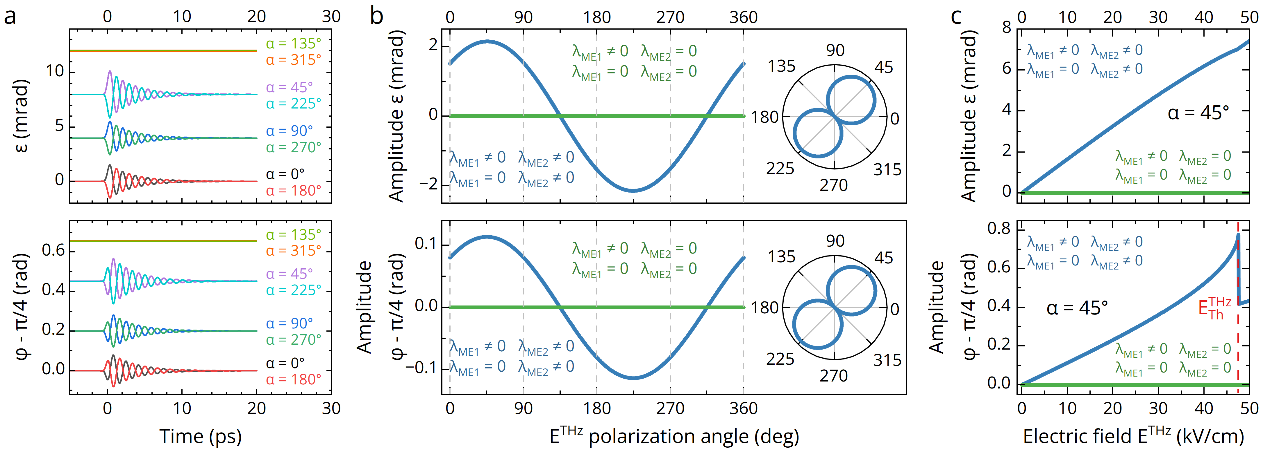
We performed simulations of the THz driven spin dynamics in Mn2Au solving the system of Eqs. (17) with the THz pump pulse described by Eq. (20). We employed the THz electric field with strength kV/cm inside the film which corresponds to the incident field about kV/cm wherever not otherwise specified. For the CuMnAs, the solved spin dynamics are qualitatively the same, but differ in magnitude. It is worth noting that we focus on studying the spin dynamics in the plane, which is described by the and variables in Eq. (17). Figure 3a shows the transients of the and for different THz pump polarization angles for a single antiferromagnetic domain with and previously defined parameters. To gain further insights, we estimated the dependence of the signed Fourier amplitude of the oscillations of and on the THz pump polarization angle . The sign of the amplitude is related to the shift of the oscillation phases. Moreover, the most pronounced oscillations of and angles are observed at polarization of the THz pump along the antiferromagnetic Néel vector at and , while the spin dynamics is not excited when and are mutually perpendicular at and (see Figs. 3a–3b).
The amplitude of oscillations of and have close to linearly dependences on the THz electric field strength inside film up to about 30 kV/cm after which these dependences become significantly nonlinear due to nonlinear spin dynamics from Eq. (17). Note that the close to linear THz electric field dependence of is consistent with experimental findings from Ref. [19]. The THz electric field polarization reversal causes a shift of the oscillation phases. These observations are consistent with the experimental results from Ref. [19] where the THz pump pulse polarized along the antiferromagnetic Néel vector with a strength of electric field estimated as 40 kV/cm on the surface of the metallic film excited a maximum deflection of the about 0.5 rad (30∘). The comparison of the simulations with these experimental results allowed us to estimate the magnetoelectric parameter which corresponds to the dimensionless magnetoelectric susceptibility for Mn2Au. This value is about an order of magnitude smaller than the value of the magnetoelectric response in prototypical antiferromagnet [40, 41, 42, 8] and many orders of magnitude less than the record values reported in [43, 44] and in other known magnetoelectrics such as [44] and [9, 45].
Next, we revealed the effects of the magnetoelectric parameters and and Zeeman torque on the oscillations of and , taking and not taking them into account when solving Eq. (17). We performed simulations of spin dynamics for two cases with , and , and we did not reveal any significant differences as shown by blue lines in Figs. 3(b) and 3(c). Besides, there is no significant spin dynamics at as seen by green lines in Figs. 3(b) and 3(c). Thus, at the employed strength of the THz pump electric field, the THz driven spin dynamics described by and is defined by the magnetoelectric parameter , whereas the parameter and Zeeman torque can be neglected. This is due to that the Zeeman torque drives the out-of-plane magnon with a frequency much higher than because .
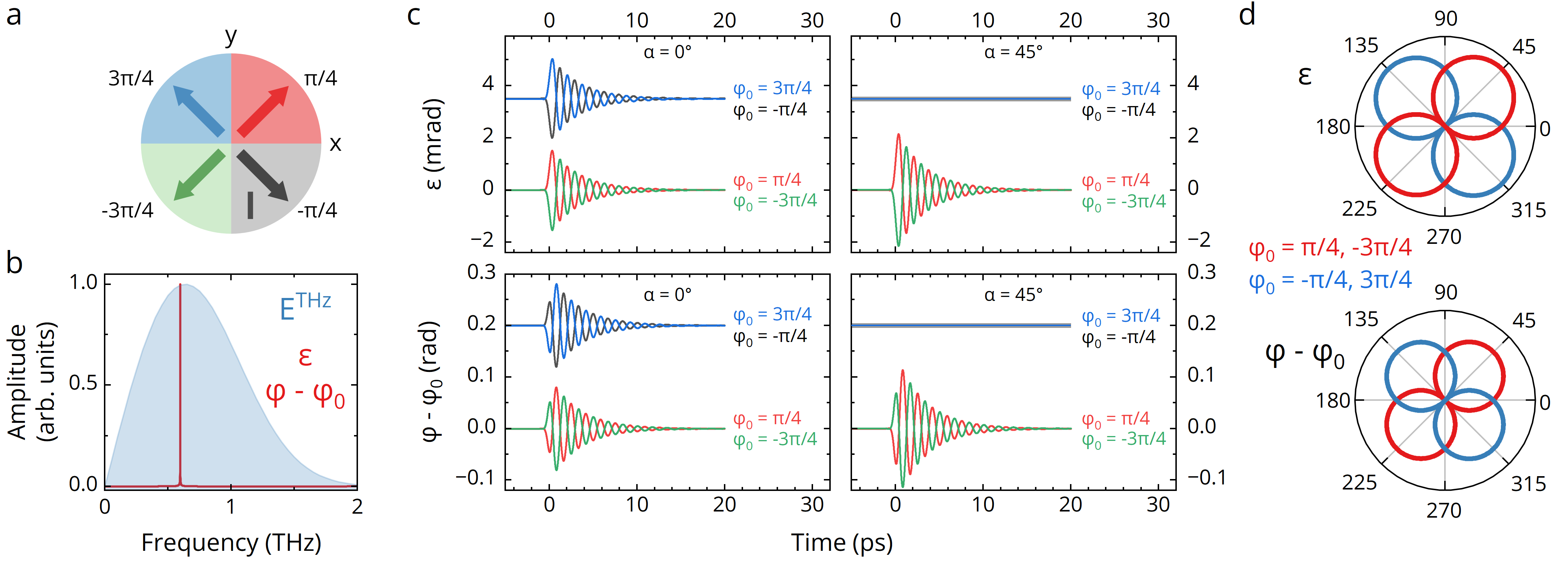
Let us discuss the features of THz driven spin dynamics in four antiferromagnetic domains in which has an angle , with respect to the axis, as sketched in Fig. 4(a). For this, we numerically solve Eq. (17) varying the initial conditions for with the previously defined parameters of Mn2Au and the THz pump pulse. Note that the frequency of oscillations for and is 0.6 THz which coincides with the maximum of the THz pump spectrum [see Fig. 4(b)]. When the THz pump is linearly polarized at , i.e., along the axis, we observe oscillations of the and with equal amplitudes in all antiferromagnetic domains, as shown in the left panels of Fig. 4(c). It is seen that the antiferromagnetic vector reversal leads to a phase shift in oscillations which was also observed for angle in the experiment [19]. Besides, when the pump is polarized perpendicular to the antiferromagnetic vector , the spin dynamics is not excited, as shown in the right panel in Fig. 4(b). In the polar diagram of the amplitudes of oscillations for and with respect to the THz pump polarization angle , it is seen that in different antiferromagnetic domains the figure eight is rotated by [see Fig. 4(c)]. Therefore, we have predicted that the THz electric field driven spin dynamics in Mn2Au has features at the crossing from one antiferromagnetic domain to another.
It was previously shown that magnetoelectric driven spin dynamics can be fairly described by considering only parameter , which allows us to significantly simplify the system of differential equations (17). Near the ground state at the polar angle and taking into account the smallness of and angles, the first two differential equations from Eq. (17) can be reduced to a next second order differential equation
| (23) |
It is worth noting that the terms quadratically dependent on the polarization are neglected from Eq. (23) because they do not significantly affect the resulting in the THz electric field range of our interest. An important consequence of Eq. (23) is that it shows that the magnetoelectric torque in metallic magnetoelectrics is proportional to the time derivative of the induced polarization (). Here one can observe a complete analogy with a Zeeman torque in collinear antiferromagnets where spin dynamics is driven by the time derivative of the effective magnetic field () [27, 46, 47, 48].
Further, if we consider the relationship between polarization and THz electric field [Eq. (22)] then Eq. (24) takes the form
| (24) |
This Eq. (24) is similar to the equation for spin dynamics driven by the Néel spin-orbit torque from Ref. [19]. In both cases the torque is proportional to the product of the conductivity by the THz electric field inside the metallic film and distinguished only in the definition of the coefficients. The linear magnetoelectric effect analyzed in this work is qualitatively similar to the Néel spin-orbit torque discussed in Ref. [19]. In the both cases, the THz electric field results in an out-of-plane magnetization which is followed by dynamics of the antiferromagnetic Néel vector in the same plane. The Néel spin-orbit torque arises from the THz electric field which leads to staggered spin-orbit fields acting on opposite magnetic sublattices [19]. The linear magnetoelectric effect resulting from the symmetry allowed term from Eq. (12). The both effects require antiferromagnets with broken inversion symmetry and strong spin-orbit coupling [49, 50, 6]. Hence, qualitatively our simulation results must be also in agreement with the experimental observations for THz driven spin dynamics in Mn2Au from Ref. [19]. It is important to mention once again that, there is absolutely no data on magnetoelectric susceptibilities in Mn2Au and in our simulations we assumed the dimensionless magnetoelectric parameter that allows us to describe the main experimental results from Ref. [19]. Also, the value of the Néel spin-orbit torque in Mn2Au at THz frequencies is not known. Hence, any quantitative comparison of the experimental results from Ref. [19] either with our simulations or with simulations from Ref. [19] is difficult. Moreover, unambiguous identification of the physical mechanism of the THz-driven spin dynamics in these materials requires further research.
5 Spin switching
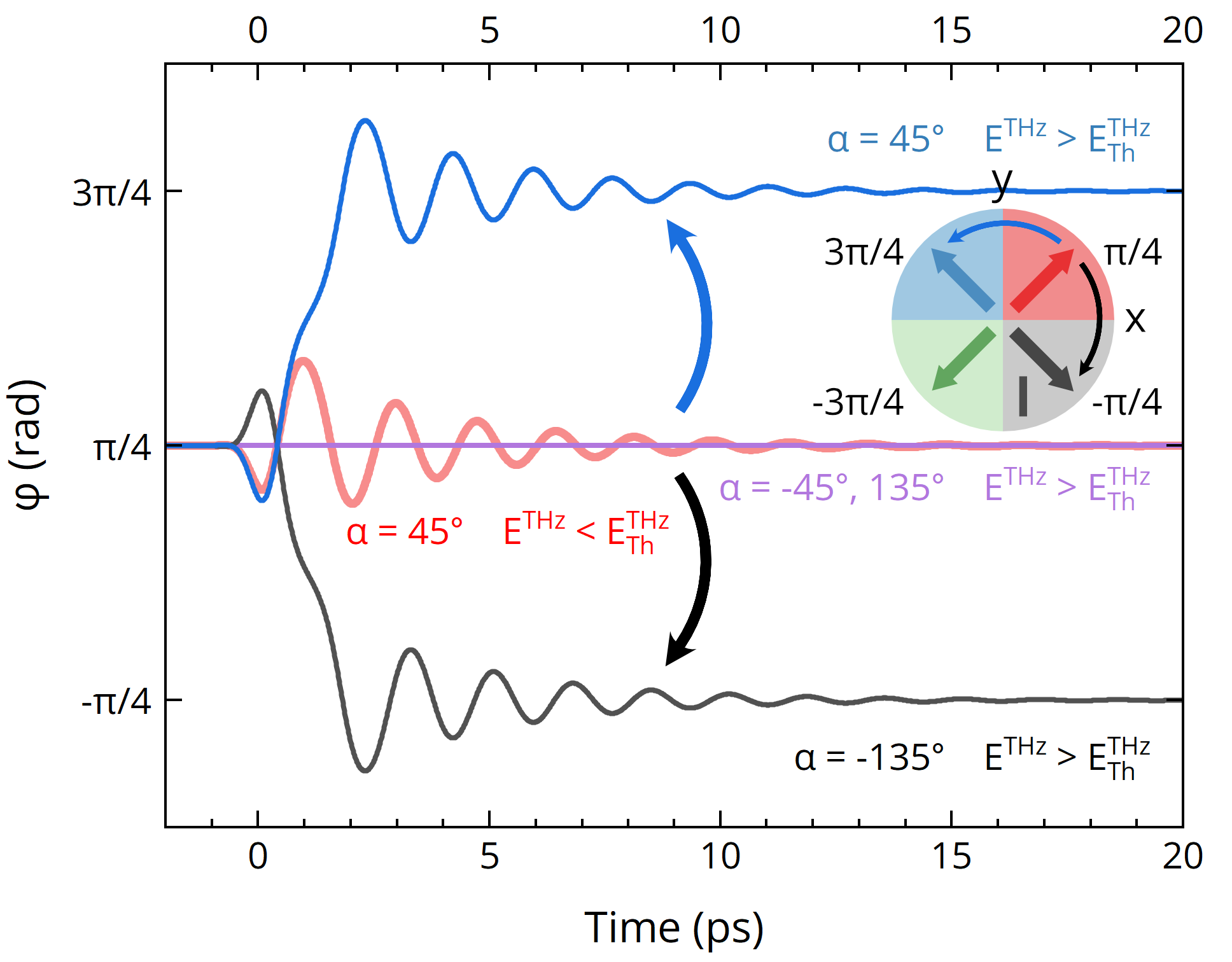
Now, we consider the switching of the antiferromagnetic vector by an applied THz electric field in Mn2Au. Numerically solving the system of Eq. (17) varying the THz electric field strength, we observed the switching of the antiferromagnetic vector from to another ground state when the field strength exceeds the threshold kV/cm inside the metallic film (see Fig. 3c), that corresponds to the incident field of about 766 kV/cm. We note that the obtained threshold THz electric field is about two times less than the estimate given in Ref. [19], which presumably is due to the difference in the shape of the THz pulse and and the way in which it is taken into account in the equation. By control of the THz polarization angle we can manipulate the final state of the antiferromagnetic Néel vector after switching. When the THz pulse is polarized at the with respect to the axis, i.e., parallel to the antiferromagnetic vector , the switching occurs from to , while at , i.e., antiparallel , the final state is already , as shown in Fig. 5. Note that the THz electric field up to MV/cm is available for tabletop setups with THz pulses generated by the tilted-front optical rectification of laser pulses in prism [33]. On the other hand, as mentioned previously, the values of the dimensionless magnetoelectric susceptibilities for Mn2Au are missing in the literature. Therefore, if the value of is about , which, however, which is a rather modest value for the linear magnetoelectric response, the switching of the antiferromagnetic Néel vector is probably possible with THz electric fields achievable in the tabletop setups.
6 Conclusions
In summary, we have discussed the spin dynamics driven by THz electric field pulses in the metallic magnetoelectric antiferromagnetic CuMnAs and Mn2Au thin films. We obtained the equations for spin dynamics and theoretically demonstrated that in the metallic antiferromagnetic magnetoelectrics the THz magnetoelectric torque is proportional to the time derivative of the induced polarization. By analyzing these equations it has been theoretically revealed that single-cycle THz pulses are able to induce the dynamics of the antiferromagnetic vector and its features in different antiferromagnetic domains are predicted. We have shown that our model is able to fairly describe the existing experimental results on the THz driven spin dynamics in the metallic Mn2Au thin film from Ref. [19] by taking into account only the linear magnetoelectric effect and not considering other mechanisms.
Thus, we have demonstrated that the linear magnetoelectric effect should be taken into consideration when discussing the THz induced spin dynamics in metallic antiferromagnetic CuMnAs and Mn2Au thin films. Moreover, it has been predicted that coherent switching of the antiferromagnetic Néel vector from one to another ground state caused by the magnetoelectric effect occurs when the THz electric field with linear polarization collinear to the antiferromagnetic vector exceeds the threshold strength. For our assumed magnetoelectric susceptibility in Mn2Au of about , the measured value of which is lacking in the literature, we reveal that the threshold THz electric field inside the metallic films is about 47.5 kV/cm, which corresponds to the incident THz pump pulse with experimentally available strength about 766 kV/cm. We hope that our results will stimulate further study of THz magnetoelectric [51, 52] and novel altermagnetoelectric [53] effects in magnetic materials, which open up the prospects for future high-speed antiferromagnetic and altermagnetic memory devices.
Declaration of competing interest
The authors declare that they have no known competing financial interests or personal relationships that could have appeared to influence the work reported in this paper. The authors declare that this work has been published as a result of peer-to-peer scientific collaboration between researchers. The provided affiliations represent the actual addresses of the authors in agreement with their digital identifier (ORCID) and cannot be considered as a formal collaboration between the aforementioned institutions.
Acknowledgements
R. M. D. acknowledges support from the Russian Science Foundation under Grant No. 24-72-00106. A. K. Z. acknowledges support from the Russian Science Foundation under Grant No. 22-12-00367. A. V. K. acknowledges support from the European Research Council ERC Grant Agreement No. 101054664 (SPARTACUS).
References
-
[1]
J. Han, R. Cheng, L. Liu, H. Ohno, S. Fukami, Coherent antiferromagnetic spintronics, Nat. Mater. 22 (6) (2023) 684–695.
doi:10.1038/s41563-023-01492-6.
URL https://doi.org/10.1038/s41563-023-01492-6 -
[2]
A. V. Kimel, A. M. Kalashnikova, A. Pogrebna, A. K. Zvezdin, Fundamentals and perspectives of ultrafast photoferroic recording, Phys. Rep. 852 (2020) 1–46.
doi:10.1016/j.physrep.2020.01.004.
URL https://doi.org/10.1016/j.physrep.2020.01.004 -
[3]
P. Němec, M. Fiebig, T. Kampfrath, A. V. Kimel, Antiferromagnetic opto-spintronics, Nat. Phys. 14 (3) (2018) 229–241.
doi:10.1038/s41567-018-0051-x.
URL https://doi.org/10.1038/s41567-018-0051-x -
[4]
V. Baltz, A. Manchon, M. Tsoi, T. Moriyama, T. Ono, Y. Tserkovnyak, Antiferromagnetic spintronics, Rev. Mod. Phys. 90 (2018) 015005.
doi:10.1103/RevModPhys.90.015005.
URL https://link.aps.org/doi/10.1103/RevModPhys.90.015005 -
[5]
T. Jungwirth, X. Marti, P. Wadley, J. Wunderlich, Antiferromagnetic spintronics, Nat. Nanotech. 11 (3) (2016) 231–241.
doi:10.1038/nnano.2016.18.
URL https://doi.org/10.1038/nnano.2016.18 -
[6]
F. Thöle, A. Keliri, N. A. Spaldin, Concepts from the linear magnetoelectric effect that might be useful for antiferromagnetic spintronics, J. Appl. Phys. 127 (21) (2020).
doi:10.1063/5.0006071.
URL https://doi.org/10.1063/5.0006071 - [7] A. K. Zvezdin, Z. V. Gareeva, Symmetry analysis of conductive antiferromagnetic materials , , Phys. Solid State 66 (6) (1997) 784–787. doi:10.61011/PSS.2024.06.58685.42HH.
- [8] E. A. Turov, A. V. Kolchanov, V. V. Menshenin, I. F. Mirsaev, V. V. Nikolaev, Symmetry and Physical Properties of Antiferromagnets, Fizmatlit, Moscow (2001).
-
[9]
M. Fiebig, Revival of the magnetoelectric effect, J. Phys. D 38 (8) (2005) R123.
doi:10.1088/0022-3727/38/8/R01.
URL https://doi.org/10.1088/0022-3727/38/8/R01 -
[10]
M. Mostovoy, Multiferroics: different routes to magnetoelectric coupling, npj Spintronics 2 (1) (2024) 18.
doi:10.1038/s44306-024-00021-8.
URL https://doi.org/10.1038/s44306-024-00021-8 -
[11]
S. D. Ganichev, E. L. Ivchenko, V. V. Bel’kov, S. A. Tarasenko, M. Sollinger, D. Weiss, W. Wegscheider, W. Prettl, Spin-galvanic effect, Nature 417 (6885) (2002) 153–156.
doi:10.1038/417153a.
URL https://doi.org/10.1038/417153a -
[12]
H. Watanabe, K. Shinohara, T. Nomoto, A. Togo, R. Arita, Symmetry analysis with spin crystallographic groups: Disentangling effects free of spin-orbit coupling in emergent electromagnetism, Phys. Rev. B 109 (2024) 094438.
doi:10.1103/PhysRevB.109.094438.
URL https://link.aps.org/doi/10.1103/PhysRevB.109.094438 -
[13]
P. Wadley, B. Howells, J. Železnỳ, C. Andrews, V. Hills, R. P. Campion, V. Novák, K. Olejník, F. Maccherozzi, S. Dhesi, et al., Electrical switching of an antiferromagnet, Science 351 (6273) (2016) 587–590.
doi:10.1126/science.aab1031.
URL https://doi.org/10.1126/science.aab1031 -
[14]
S. Y. Bodnar, L. Šmejkal, I. Turek, T. Jungwirth, O. Gomonay, J. Sinova, A. A. Sapozhnik, H.-J. Elmers, M. Kläui, M. Jourdan, Writing and reading antiferromagnetic by Néel spin-orbit torques and large anisotropic magnetoresistance, Nat. Commun. 9 (1) (2018) 348.
doi:10.1038/s41467-017-02780-x.
URL https://doi.org/10.1038/s41467-017-02780-x -
[15]
A. M. Poletaeva, A. I. Nikitchenko, N. A. Pertsev, Néel Vector Auto-Oscillations and Reorientations Induced by Spin-Polarized Electric Currents in Antiferromagnetic Nanolayer, SPIN 14 (4) (2024) 2450017.
doi:10.1142/S2010324724500176.
URL https://doi.org/10.1142/S2010324724500176 -
[16]
Z. Kašpar, M. Surỳnek, J. Zubáč, F. Krizek, V. Novák, R. P. Campion, M. S. Wörnle, P. Gambardella, X. Marti, P. Němec, K. W. Edmonds, S. Reimers, O. J. Amin, F. Maccherozzi, S. S. Dhesi, P. Wadley, J. Wunderlich, K. Olejník, T. Jungwirth, Quenching of an antiferromagnet into high resistivity states using electrical or ultrashort optical pulses, Nat. Electron. 4 (1) (2021) 30–37.
doi:10.1038/s41928-020-00506-4.
URL https://doi.org/10.1038/s41928-020-00506-4 -
[17]
K. Olejník, Z. Kašpar, J. Zubáč, S. Telkamp, A. Farkaš, D. Kriegner, K. Vỳbornỳ, J. Železnỳ, Z. Šobáň, P. Zeng, et al., Quench switching of , arXiv preprint arXiv:2411.01930 (2024).
doi:10.48550/arXiv.2411.01930.
URL https://doi.org/10.48550/arXiv.2411.01930 -
[18]
J. Heitz, L. Nádvorník, V. Balos, Y. Behovits, A. Chekhov, T. Seifert, K. Olejník, Z. Kašpar, K. Geishendorf, V. Novák, R. Campion, M. Wolf, T. Jungwirth, T. Kampfrath, Optically Gated Terahertz-Field-Driven Switching of Antiferromagnetic , Phys. Rev. Appl. 16 (2021) 064047.
doi:10.1103/PhysRevApplied.16.064047.
URL https://link.aps.org/doi/10.1103/PhysRevApplied.16.064047 -
[19]
Y. Behovits, A. L. Chekhov, S. Y. Bodnar, O. Gueckstock, S. Reimers, Y. Lytvynenko, Y. Skourski, M. Wolf, T. S. Seifert, O. Gomonay, M. Kläui, M. Jourdan, T. Kampfrath, Terahertz néel spin-orbit torques drive nonlinear magnon dynamics in antiferromagnetic , Nat. Commun. 14 (1) (2023) 6038.
doi:10.1038/s41467-023-41569-z.
URL https://doi.org/10.1038/s41467-023-41569-z -
[20]
P. Wadley, V. Novák, R. Campion, C. Rinaldi, X. Martí, H. Reichlová, J. Železný, J. Gazquez, M. Roldan, M. Varela, D. Khalyavin, S. Langridge, D. Kriegner, F. Máca, J. Mašek, R. Bertacco, V. Holý, A. Rushforth, K. Edmonds, B. Gallagher, C. Foxon, J. Wunderlich, T. Jungwirth, Tetragonal phase of epitaxial room-temperature antiferromagnet , Nat. Commun. 4 (1) (2013) 2322.
doi:10.1038/ncomms3322.
URL https://doi.org/10.1038/ncomms3322 -
[21]
V. M. T. S. Barthem, C. V. Colin, H. Mayaffre, M.-H. Julien, D. Givord, Revealing the properties of for antiferromagnetic spintronics, Nat. Commun. 4 (1) (2013) 2892.
doi:10.1038/ncomms3892.
URL https://doi.org/10.1038/ncomms3892 -
[22]
P. Wadley, V. Hills, M. R. Shahedkhah, K. W. Edmonds, R. P. Campion, V. Novák, B. Ouladdiaf, D. Khalyavin, S. Langridge, V. Saidl, P. Nemec, A. W. Rushforth, B. L. Gallagher, S. S. Dhesi, F. Maccherozzi, J. Železný, T. Jungwirth, Antiferromagnetic structure in tetragonal thin films, Sci. Rep. 5 (1) (2015) 17079.
doi:10.1038/srep17079.
URL https://doi.org/10.1038/srep17079 -
[23]
T. B. Massalski, H. Okamoto, The Au-Mn (Gold-Manganese) system, Bull. Alloy Phase Diagrams 6 (5) (1985) 454–467.
doi:10.1007/bf02869510.
URL http://dx.doi.org/10.1007/BF02869510 -
[24]
M. S. Gebre, R. K. Banner, K. Kang, K. Qu, H. Cao, A. Schleife, D. P. Shoemaker, Magnetic anisotropy in single-crystalline antiferromagnetic , Phys. Rev. Mater. 8 (2024) 084413.
doi:10.1103/PhysRevMaterials.8.084413.
URL https://link.aps.org/doi/10.1103/PhysRevMaterials.8.084413 -
[25]
M. S. Gebre, R. K. Banner, K. Kang, K. Qu, H. Cao, A. Schleife, D. P. Shoemaker, Magnetic anisotropy in single-crystalline antiferromagnetic , Phys. Rev. Mater. 8 (2024) 084413.
doi:10.1103/PhysRevMaterials.8.084413.
URL https://link.aps.org/doi/10.1103/PhysRevMaterials.8.084413 -
[26]
S. Reimers, O. Gomonay, O. J. Amin, F. Krizek, L. X. Barton, Y. Lytvynenko, S. F. Poole, V. Novák, R. P. Campion, F. Maccherozzi, G. Carbone, A. Björling, Y. Niu, E. Golias, D. Kriegner, J. Sinova, M. Kläui, M. Jourdan, S. S. Dhesi, K. W. Edmonds, P. Wadley, Magnetic domain engineering in antiferromagnetic and , Phys. Rev. Appl. 21 (2024) 064030.
doi:10.1103/PhysRevApplied.21.064030.
URL https://link.aps.org/doi/10.1103/PhysRevApplied.21.064030 -
[27]
A. K. Zvezdin, Dynamics of domain walls in weak ferromagnets, JETP Lett. 29 (10) (1979) 553–556.
URL http://jetpletters.ru/ps/1456/article_22180.shtml -
[28]
A. K. Zvezdin, Dynamics of domain walls in weak ferromagnets, arXiv preprint arXiv:1703.01502 (2017).
doi:arXiv:1703.01502v1.
URL https://doi.org/10.48550/arXiv.1703.01502 -
[29]
A. K. Zvezdin, R. M. Dubrovin, A. V. Kimel, Giant Parametric Amplification of the Inverse Cotton–Mouton Effect in Antiferromagnetic Crystals, JETP Lett. 119 (5) (2024) 363–371.
doi:10.1134/S0021364023604050.
URL https://doi.org/10.1134/S0021364023604050 - [30] E. Fradkin, Field theories of condensed matter physics, Cambridge University Press, 2013.
-
[31]
T. W. Metzger, K. A. Grishunin, C. Reinhoffer, R. M. Dubrovin, A. Arshad, I. Ilyakov, T. V. de Oliveira, A. Ponomaryov, J.-C. Deinert, S. Kovalev, R. V. Pisarev, M. I. Katsnelson, B. A. Ivanov, P. H. van Loosdrecht, A. V. Kimel, E. A. Mashkovich, Magnon-phonon fermi resonance in antiferromagnetic , Nat. Commun. 15 (1) (2024) 5472.
doi:10.1038/s41467-024-49716-w.
URL https://doi.org/10.1038/s41467-024-49716-w -
[32]
T. G. H. Blank, K. A. Grishunin, K. A. Zvezdin, N. T. Hai, J. C. Wu, S.-H. Su, J.-C. A. Huang, A. K. Zvezdin, A. V. Kimel, Two-dimensional terahertz spectroscopy of nonlinear phononics in the topological insulator , Phys. Rev. Lett. 131 (2023) 026902.
doi:10.1103/PhysRevLett.131.026902.
URL https://link.aps.org/doi/10.1103/PhysRevLett.131.026902 -
[33]
E. A. Mashkovich, K. A. Grishunin, R. M. Dubrovin, A. K. Zvezdin, R. V. Pisarev, A. V. Kimel, Terahertz light-driven coupling of antiferromagnetic spins to lattice, Science 374 (2021) 1608–1611.
doi:10.1126/science.abk1121.
URL https://doi.org/10.1126/science.abk1121 - [34] L. Landau, E. Lifshitz, Electrodynamics of continuous media, Vol. 8, Pergamon, 1984.
-
[35]
A. Thoman, A. Kern, H. Helm, M. Walther, Nanostructured gold films as broadband terahertz antireflection coatings, Phys. Rev. B 77 (2008) 195405.
doi:10.1103/PhysRevB.77.195405.
URL https://link.aps.org/doi/10.1103/PhysRevB.77.195405 -
[36]
M. Wang, C. Andrews, S. Reimers, O. J. Amin, P. Wadley, R. P. Campion, S. F. Poole, J. Felton, K. W. Edmonds, B. L. Gallagher, A. W. Rushforth, O. Makarovsky, K. Gas, M. Sawicki, D. Kriegner, J. Zubáč, K. Olejník, V. Novák, T. Jungwirth, M. Shahrokhvand, U. Zeitler, S. S. Dhesi, F. Maccherozzi, Spin flop and crystalline anisotropic magnetoresistance in cumnas, Phys. Rev. B 101 (2020) 094429.
doi:10.1103/PhysRevB.101.094429.
URL https://link.aps.org/doi/10.1103/PhysRevB.101.094429 -
[37]
M. Arana, F. Estrada, D. S. Maior, J. B. S. Mendes, L. E. Fernandez-Outon, W. A. A. Macedo, V. M. T. S. Barthem, D. Givord, A. Azevedo, S. M. Rezende, Observation of magnons in films by inelastic Brillouin and Raman light scattering, Appl. Phys. Lett. 111 (19) (2017).
doi:10.1063/1.5001705.
URL https://doi.org/10.1063/1.5001705 -
[38]
N. Bhattacharjee, A. A. Sapozhnik, S. Y. Bodnar, V. Y. Grigorev, S. Y. Agustsson, J. Cao, D. Dominko, M. Obergfell, O. Gomonay, J. Sinova, M. Kläui, H.-J. Elmers, M. Jourdan, J. Demsar, Néel Spin-Orbit Torque Driven Antiferromagnetic Resonance in Probed by Time-Domain THz Spectroscopy, Phys. Rev. Lett. 120 (2018) 237201.
doi:10.1103/PhysRevLett.120.237201.
URL https://link.aps.org/doi/10.1103/PhysRevLett.120.237201 -
[39]
A. B. Shick, S. Khmelevskyi, O. N. Mryasov, J. Wunderlich, T. Jungwirth, Spin-orbit coupling induced anisotropy effects in bimetallic antiferromagnets: A route towards antiferromagnetic spintronics, Phys. Rev. B 81 (2010) 212409.
doi:10.1103/PhysRevB.81.212409.
URL https://link.aps.org/doi/10.1103/PhysRevB.81.212409 -
[40]
D. N. Astrov, The magnetoelectric effect in antiferromagnetics, Sov. Phys. JETP 11 (3) (1960) 708–709.
URL http://www.jetp.ras.ru/cgi-bin/dn/e_011_03_0708.pdf -
[41]
D. N. Astrov, Magnetoelectric effect in chromium oxide, Sov. Phys. JETP 13 (4) (1961) 729–733.
URL http://jetp.ras.ru/cgi-bin/dn/e_013_04_0729.pdf -
[42]
G. T. Rado, V. J. Folen, Observation of the Magnetically Induced Magnetoelectric Effect and Evidence for Antiferromagnetic Domains, Phys. Rev. Lett. 7 (1961) 310–311.
doi:10.1103/PhysRevLett.7.310.
URL https://link.aps.org/doi/10.1103/PhysRevLett.7.310 -
[43]
Y. Tokunaga, S. Iguchi, T. Arima, Y. Tokura, Magnetic-Field-Induced Ferroelectric State in , Phys. Rev. Lett. 101 (2008) 097205.
doi:10.1103/PhysRevLett.101.097205.
URL https://link.aps.org/doi/10.1103/PhysRevLett.101.097205 -
[44]
E. Bousquet, A. Cano, Non-collinear magnetism in multiferroic perovskites, J. Phys. Condens. Matter 28 (12) (2016) 123001.
doi:10.1088/0953-8984/28/12/123001.
URL https://doi.org/10.1088/0953-8984/28/12/123001 -
[45]
J.-P. Rivera, A short review of the magnetoelectric effect and related experimental techniques on single phase (multi-) ferroics, Eur. Phys. J. B 71 (2009) 299–313.
doi:10.1140/epjb/e2009-00336-7.
URL https://doi.org/10.1140/epjb/e2009-00336-7 -
[46]
A. F. Andreev, V. I. Marchenko, Symmetry and the macroscopic dynamics of magnetic materials, Sov. Phys. Usp. 130 (1980) 39.
doi:10.1070/PU1980v023n01ABEH004859.
URL https://doi.org/10.1070/PU1980v023n01ABEH004859 - [47] A. K. Zvezdin, A. A. Mukhin, New nonlinear dynamics effects in antiferromagnets, Bull. Lebedev Phys. Inst. 12 (1981) 10.
-
[48]
T. Satoh, S.-J. Cho, R. Iida, T. Shimura, K. Kuroda, H. Ueda, Y. Ueda, B. A. Ivanov, F. Nori, M. Fiebig, Spin Oscillations in Antiferromagnetic Triggered by Circularly Polarized Light, Phys. Rev. Lett. 105 (2010) 077402.
doi:10.1103/PhysRevLett.105.077402.
URL https://link.aps.org/doi/10.1103/PhysRevLett.105.077402 - [49] I. E. Dzyaloshinskii, On the magneto-electrical effects in antiferromagnets, Sov. Phys. JETP 10 (1960) 628–629. doi:http://jetp.ras.ru/cgi-bin/dn/e_010_03_0628.pdf.
-
[50]
J. Železný, H. Gao, K. Výborný, J. Zemen, J. Mašek, A. Manchon, J. Wunderlich, J. Sinova, T. Jungwirth, Relativistic Néel-Order Fields Induced by Electrical Current in Antiferromagnets, Phys. Rev. Lett. 113 (2014) 157201.
doi:10.1103/PhysRevLett.113.157201.
URL https://link.aps.org/doi/10.1103/PhysRevLett.113.157201 -
[51]
F. Y. Gao, X. Peng, X. Cheng, E. Viñas Boström, D. S. Kim, R. K. Jain, D. Vishnu, K. Raju, R. Sankar, S.-F. Lee, M. A. Sentef, T. Kurumaji, X. Li, P. Tang, A. Rubio, E. Baldini, Giant chiral magnetoelectric oscillations in a van der Waals multiferroic, Nature 632 (8024) (2024) 273–279.
doi:10.1038/s41586-024-07678-5.
URL https://doi.org/10.1038/s41586-024-07678-5 -
[52]
K.-X. Zhang, G. Park, Y. Lee, B. H. Kim, J.-G. Park, Magnetoelectric effect in van der waals magnets, npj Quantum Mater. 10 (1) (2025) 6.
doi:10.1038/s41535-025-00725-y.
URL https://doi.org/10.1038/s41535-025-00725-y -
[53]
L. Šmejkal, Altermagnetic multiferroics and altermagnetoelectric effect, arXiv preprint arXiv:2411.19928 (2024).
doi:10.48550/arXiv.2411.19928.
URL https://doi.org/10.48550/arXiv.2411.19928