Structure, Positivity and Classical Simulability of Kirkwood–Dirac Distributions

Abstract

The Kirkwood-Dirac (KD) quasiprobability distribution is known for its role in quantum metrology, thermodynamics, as well as the foundations of quantum mechanics. Here, we study the superoperator evolution of KD distributions and show that unitaries which preserve KD positivity do not always correspond to a stochastic evolution of quasiprobabilities. Conversely, we show that stochastic KD superoperators are always induced by generalised permutations within the KD reference bases. We identify bounds for pure KD positive states in distributions defined on mutually unbiased bases, showing that they always form uniform distributions, in full analogy to the stabilizer states. Subsequently, we show that the discrete Fourier transform of KD distributions on qudits in the Fourier basis follows a self-similarity constraint and provides the expectation values of the state with respect to the Weyl-Heisenberg unitaries, which can then be transformed into the (odd-dimensional) Wigner distribution. This defines a direct mapping between the Wigner, and qudit KD distributions without a reconstruction of the density matrix. Finally, we identify instances where the classical sampling-based simulation algorithm of Pashayan et al. [Phys. Rev. Lett. 115, 070501] becomes exponentially inefficient in spite of the state being KD positive throughout its evolution.

I Introduction

Concurrent developments in quantum computation and quantum information theory have brought forward a variety of cross-applicable tools, to the enjoyment of researchers in both fields. For physicists looking to study quantum phenomena in complex systems, error-correcting codes have established themselves as a powerful framework for describing topological phases of matter [1, 2, 3]. In quantum metrology, ideas from quantum hypothesis testing have formed a theoretical underpinning of various quantum sensing protocols [4, 5]. Conversely, the notion of a quasiprobability distribution – originally confined to the field of quantum optics – has become a popular paradigm for theorists looking to understand when a quantum system achieves computational advantage [6, 7, 8, 9, 10, 11, 12, 13, 14]. With the landmark paper of Gross [15], the discrete Wigner distribution took on a central role for Clifford quantum computation. An alternative formalism – the Kirkwood-Dirac (KD) distribution [16, 17] – has recently undergone a revival, with very successful applications to quantum metrology [18, 19, 20, 21, 22, 23], thermodynamics [24, 25, 26, 27, 28, 29], and identifying quantum non-contextuality [30, 31, 32, 33] (see [34] for a comprehensive review). However, the KD distribution has received little attention in the context of quantum computation: despite frequent assertions that KD distributions are related to the Wigner distribution, very little is known about how the two relate mathematically or what role KD negativity can play in achieving a computational quantum advantage. In this work, we address this question and provide analogies and differences between the two distributions. Our investigation is three-fold: we first consider the phase space evolution of KD distributions under unitary quantum channels, showing that the Hudson theorem [15] does not fully apply in their setting. We then study classical simulations of quantum circuits using KD distributions, showing that the absence of the Hudson theorem leads to unexpected complications in linking computational advantage to KD non-positivity. Finally, we relate the two distributions mathematically, showing that certain instances of KD distributions are indeed a close relative of the Wigner distribution, related by discrete Fourier transforms of Weyl-Heisenberg expectation values. The relationship turns out to be intricate, as despite many differences, some KD positive states still feature properties mirroring those of stabilizer states.

The article is structured as follows: In Section II, we review the Kirkwood-Dirac distribution and its properties, and outline the recent developments which we build upon. Following this, in Section III we introduce the vectorisation of KD distributions, in which distribution matrices are promoted to vectors, and their evolution to matrix multiplication by appropriate quasi-stochastic matrices. We then derive the superoperator elements for general CPTP maps and unitary quantum channels, and offer a new method for their experimental measurement using a generalisation of the cycle test [35, 36]. This leads into Section IV, in which we use the superoperator elements to identify the full set of unitaries $U$ which induce stochastic KD superoperators, and prove that these are generalised permutations acting on the KD reference bases (Theorems 1, 2). Whilst such unitaries have the property of always preserving the KD positivity of a state, they are not the only unitaries which do so, as we demonstrate with a few simple examples. This is contrasted to the discrete Wigner distribution, where positivity-preservation of the Clifford gates is synonymous with stochasticity of their superoperators. In Section V we investigate the consequences of this for the classical simulation of quantum circuits using KD distributions. To do so, we adapt a well-known algorithm for Born rule probability estimation of [14]: as the algorithm relies on stochasticity of positivity-preserving quantum channels to be efficient, we identify a significant problem for the prospects of quantum simulation in the KD setting: a quantum state can be KD positive throughout its evolution, yet take exponentially long to simulate. In Section VI, we offer some insights into why this is so, and in the process identify a new set of $d^{2}$ constraints on KD distributions representing valid quantum states. This culminates in Theorem 3, in which we apply our constraints to distributions defined on bases related by a quantum Fourier transform (QFT), and show that they gives rise to a self-similarity property of the discrete Fourier transforms (DFTs) of the distributions themselves. In this sense, the DFT of such a distribution can be said to ‘condense’ the information about a state into a subset of its elements. In turn, Section VII provides a new prescription on how to use the DFT to transform between KD distributions defined on QFTs, the expectation values of the Weyl-Heisenberg (WH) unitaries, and the discrete Wigner distribution without a need to reconstruct the underlying density matrix. The Wigner distribution is known to be a symplectic Fourier transform of the WH expectation values – our findings show that a similar relationship holds for certain instances of the KD distribution. Finally, in Section VIII we offer new bounds on the magnitudes of quasiprobabilities for any KD distribution (Theorem 52), with the corollary that for distributions defined on mutually unbiased bases (MUBs) the KD positive states form a uniform distribution over their support (Theorem 5) – a result completely analogous to the uniform distribution in the Wigner distribution of stabilizer states. At the end of each section we make comparisons between our findings and known properties of Wigner distributions, which are summarised (along with other relevant facts) in Table 3.

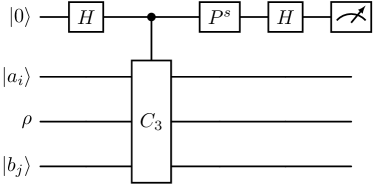
(a)

(b)

Figure 1: Left: The cycle test for estimating $\text{Re}[Q_{ij}(\rho)]$ ($s=0$), and $\text{Im}[Q_{ij}(\rho)]$ ($s=1$). $H$ is the Hadamard gate, and $P=\text{diag}(1,i)$. After many measurements, $Q_{ij}(\rho)$ is estimated from the outcome frequencies via $p_{s=0}(0)=(1+\text{Re}[Q_{ij}])/2$ and $p_{s=1}(0)=(1+\text{Im}[Q_{ij}])/2$. Right: The cycle gate may be implemented by a cascade of qudit controlled-$SWAP$ gates.

II Preliminaries

Kirkwood-Dirac Distributions. In this paper, we will consider the ‘standard’, KD distributions, defined with respect to two orthonormal bases $\mathcal{A}=\{|a_{i}\rangle\}_{i\in\llbracket d\rrbracket}$. and $\mathcal{B}=\{|b_{j}\rangle\}_{j\in\llbracket d\rrbracket}$ of a $d$-dimensional Hilbert space $\mathcal{H}_{d}$ (Here and throughout, $\llbracket d\rrbracket=\{1,...,d\}$ refers to a set of integers from $1$ to $d$). For a quantum state $\rho\in\mathcal{H}_{d}$, the KD distribution offers a description of $\rho$ in terms of a set of $d^{2}$ quasiprobabilities $Q_{ij}(\rho)$, which are complex numbers defined as [34]:

$$Q_{ij}(\rho)=\langle b_{j}|a_{i}\rangle\langle a_{i}|\rho|b_{j}\rangle,\ \text{where }\ (i,j)\in\llbracket d\rrbracket^{2}.$$ (1)

The name ‘quasiprobability’ arises from the fact that the quantities $Q_{ij}(\rho)$ satisfy some, but not all of the Kolmogorov axioms. For instance, they sum to $1$ and correctly reproduce Born rule probabilities upon marginalisation:

$$\sum_{j}Q_{ij}(\rho) =\langle a_{i}|\rho|a_{i}\rangle, \sum_{i}Q_{ij}(\rho) =\langle b_{j}|\rho|b_{j}\rangle.$$ (2)

As the KD distribution is invariant under a global change of basis (where $|a_{i}\rangle\rightarrow U|a_{i}\rangle$, $|b_{j}\rangle\rightarrow U|b_{j}\rangle$, $\rho\rightarrow U\rho U^{\dagger}$), it is often convenient to take $\{|a_{i}\rangle\}$ to be the computational basis, and $|b_{j}\rangle=V|a_{j}\rangle$ for some unitary transition matrix $V$. One can also define the KD distribution in terms of frames $\Lambda_{ij}$, satisfying:

$$\Lambda_{ij} =\frac{|a_{i}\rangle\langle b_{j}|}{\langle b_{j}|a_{i}\rangle}, Q_{ij}(\rho) =\frac{\text{Tr}(\Lambda_{ij}^{\dagger}\rho)}{\text{Tr}(\Lambda_{ij}\Lambda_{ij}^{\dagger})},$$ (3)

where the possibility of complex-valued $Q_{ij}(\rho)$ can be directly seen as a consequence of the non-hermicity of $\Lambda_{ij}$. The frames enable one to then reconstruct $\rho$ via the weighed sum:

$$\rho=\sum_{ij}Q_{ij}(\rho)\Lambda_{ij}.$$ (4)

This is only possible if $m_{\mathcal{A,B}}=\min_{ij}|\langle a_{i}|b_{j}\rangle|>0$, in which case we say that the KD distribution is informationally complete. This corresponds to the transition matrix $V$ having zero sparsity. In this work we will assume informational completeness, and state otherwise when needed. For mutually unbiased bases (MUBs), $|\langle a_{i}|b_{j}\rangle|=m_{\mathcal{A,B}}=1/\sqrt{d}$ for all $i,j$, and the corresponding $V$ is a complex Hadamard matrix.

KD Positivity. When a KD distribution takes on exclusively real non-negative values, it resembles a classical joint probability distribution. In those cases we say that it is KD positive, or KD classical. Given that all KD distributions sum to $1$, a popular measure of KD positivity is the total non-positivity, defined as:

$$\mathcal{N}(Q(\rho))=\sum_{ij}|Q_{ij}(\rho)|\geq 1,$$ (5)

where the distribution is KD positive if and only if $\mathcal{N}(Q(\rho))=1$. KD non-positivity has been linked to non-classical phenomena in quantum non-contextuality, advantages in quantum metrology, and more. One set of pure KD positive states are the bases $\mathcal{A,B}$ themselves, for which $Q_{ij}(a_{k})=\delta_{ki}|\langle a_{k}|b_{j}\rangle|^{2}$ (and similarly for $Q_{ij}(b_{m})$). Recent work [37] has shown that for the vast majority of KD distributions (i.e. with probability 1, when $V$ is sampled via the Haar measure on $\mathbb{C}^{d\times d}$), the basis states from $\mathcal{A,B}$ are the only KD positive pure states. Nonetheless, for some choices of $V$ pure, non-trivial KD positive states exist, and there are also mixed KD positive states lying outside of the convex set of pure KD positive states [38].

Support Uncertainties. For a pure state $|\psi\rangle$ described on a KD distribution it is also useful to define the support uncertainties $n_{\mathcal{A}},n_{\mathcal{B}}$, which count the number of non-zero inner products between $|\psi\rangle$ and the two respective bases:

$$n_{\mathcal{A}} =|S_{\mathcal{A}}|=|\{|a_{i}\rangle\in\mathcal{A}:\langle a_{i}|\psi\rangle\neq 0\}|,$$

$$n_{\mathcal{B}} =|S_{\mathcal{B}}|=|\{|b_{j}\rangle\in\mathcal{B}:\langle b_{j}|\psi\rangle\neq 0\}|.$$ (6)

The product $n_{\mathcal{A}}n_{\mathcal{B}}$ is then the number of non-zero entries in the KD distribution $Q_{ij}(\psi)$, i.e. its support. Other authors have shown [39] that for all pure KD positive states, the sum $n_{\mathcal{A}}+n_{\mathcal{B}}$ satisfies:

$$n_{\mathcal{A}}+n_{\mathcal{B}}\leq d+1,$$ (7)

and that for MUBs, all pure KD positive states also satisfy [40, 38]:

$$n_{\mathcal{A}}n_{\mathcal{B}}=d.$$ (8)

Experimental Measurement of KD Distributions. Directly sampling from an unknown KD distribution on a given state $\rho$ is a challenging endeavour. As $Q_{ij}(\rho)=\text{Tr}(|b_{j}\rangle\langle b_{j}|a_{i}\rangle\langle a_{i}|\rho)$, one cannot devise a procedure which returns outcomes $(i,j)$ with probabilities $Q_{ij}(\rho)$, as the outer products $\langle b_{j}|a_{i}\rangle\times|b_{j}\rangle\langle a_{i}|$ do not form valid POVM elements. Nonetheless, Wagner et. al. [35] (using a circuit first introduced by Oszmaniec et. al. [36]) have provided a procedure for estimating the quasiprobabilities $Q_{ij}(\rho)$ using a generalisation of the SWAP test known as the cycle test. The circuit is shown in Figure 1. In the next section, we extend this protocol to provide a new method for experimental calculations of KD superoperator elements $(\hat{\mathcal{E}}_{U})_{ij,kl}$ induced by an unknown unitary $U$ and any informationally complete choice of bases $\mathcal{A,B}$.

For an excellent recent review of KD distributions and their applications discussing all of the above in more detail, the reader is encouraged to consult [34].

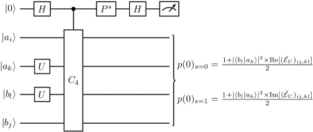
Figure 2: A cycle test for estimating the KD superoperator matrix elements $|\langle b_{l}|a_{k}\rangle|^{2}\times(\hat{\mathcal{E}}_{U})_{ij,kl}$. The quantity $|\langle b_{l}|a_{k}\rangle|^{2}$ may be estimated separately, using the SWAP test.

III Vectorisation of Kirkwood-Dirac Distributions

KD Distributions as Vectors. Our approach is motivated by the common practice of representing quantum states $\rho\in\mathbb{C}^{d\times d}$ as vectors in $\mathbb{C}^{d^{2}}$, often referred to as the vectorisation of $\rho$. This was first done for KD distributions in a recent paper [32], albeit with differences in notation – before moving onto the main results, we will outline and build on key concepts. We proceed by stacking the rows of a KD distribution matrix $Q(\rho)$ into a single column vector, as follows:

$$Q(\rho)=\begin{pmatrix}Q_{11}&\ldots&Q_{1d}\\ \vdots&\ddots&\vdots\\ Q_{d1}&\ldots&Q_{dd}\end{pmatrix}\ \rightarrow\ \boldsymbol{|}Q(\rho)\boldsymbol{\rangle\rangle}=\begin{pmatrix}Q_{11}\\ Q_{12}\\ \vdots\\ Q_{1d}\\ Q_{21}\\ \vdots\\ Q_{dd}\end{pmatrix}.$$ (9)

It is also useful to define the vector $\boldsymbol{\langle\langle 1|}$, which belongs to the dual space:

$$\boldsymbol{\langle\langle 1|}=\begin{pmatrix}1&1&\ldots&1\end{pmatrix}.$$ (10)

Clearly, all KD distribution vectors satisfy $\boldsymbol{\langle\langle 1|}Q(\rho)\boldsymbol{\rangle\rangle}=1$. The total non-positivity of a KD distribution can then be written as the $l_{1}$ norm of $\boldsymbol{|}Q(\rho)\boldsymbol{\rangle\rangle}$:

$$\mathcal{N}(Q(\rho))=\|\boldsymbol{|}Q(\rho)\boldsymbol{\rangle\rangle}\|_{1}.$$ (11)

KD Superoperators. Here we consider the evolution of a KD distribution $Q(\rho)\rightarrow Q(\mathcal{E}(\rho))$ under a quantum channel (a completely positive, trace-preserving map) $\mathcal{E}$ acting on $\rho$. In the larger space $\mathbb{C}^{d^{2}\times d^{2}}$, this may be written as the multiplication of $\boldsymbol{|}Q(\rho)\boldsymbol{\rangle\rangle}$ by a $d^{2}\times d^{2}$ matrix $\hat{\mathcal{E}}$:

$$\boldsymbol{|}Q(\mathcal{E}(\rho))\boldsymbol{\rangle\rangle}=\hat{\mathcal{E}}\boldsymbol{|}Q(\rho)\boldsymbol{\rangle\rangle}.$$ (12)

If $\mathcal{E}$ is composed of a set of Kraus operators $\{K_{\mu}\}$ (such that $\sum_{\mu}K^{\dagger}_{\mu}K_{\mu}=\mathbb{1}_{d}$), then the quasiprobabilities $Q_{ij}$ evolve as follows:

$$Q_{ij} \rightarrow\sum_{\mu}\langle b_{j}|a_{i}\rangle\times\langle a_{i}|K_{\mu}\rho K_{\mu}^{\dagger}|b_{j}\rangle$$

$$=\sum_{\mu}\sum_{kl}\langle b_{j}|a_{i}\rangle\times\langle a_{i}|K_{\mu}|a_{k}\rangle\langle a_{k}|\rho|b_{l}\rangle\langle b_{l}|K_{\mu}^{\dagger}|b_{j}\rangle$$

$$=\sum_{kl}\left(\sum_{\mu}\frac{\langle b_{j}|a_{i}\rangle}{\langle b_{l}|a_{k}\rangle}\langle a_{i}|K_{\mu}|a_{k}\rangle\langle b_{l}|K_{\mu}^{\dagger}|b_{j}\rangle\right)\times Q_{kl}$$

$$=\sum_{kl}\hat{\mathcal{E}}_{ij,kl}Q_{kl}.$$ (13)

This allows us to identify the matrix elements $\hat{\mathcal{E}}_{ij,kl}$:

$$\hat{\mathcal{E}}_{ij,kl} =\sum_{\mu}\frac{\langle b_{j}|a_{i}\rangle}{\langle b_{l}|a_{k}\rangle}\langle a_{i}|K_{\mu}|a_{k}\rangle\langle b_{l}|K_{\mu}^{\dagger}|b_{j}\rangle$$

$$=\sum_{\mu}\frac{\text{Tr}(\Lambda_{ij}^{\dagger}K_{\mu}\Lambda_{kl}K_{\mu}^{\dagger})}{\text{Tr}(\Lambda_{ij}\Lambda_{ij}^{\dagger})}.$$ (14)

We can explicitly see that $\hat{\mathcal{E}}$ maps KD vectors to valid KD vectors. This is because its columns sum to 1:

$$\sum_{ij}\hat{\mathcal{E}}_{ij,kl} =\frac{1}{\langle b_{l}|a_{k}\rangle}\sum_{ij}\sum_{\mu}\langle b_{l}|K_{\mu}^{\dagger}|b_{j}\rangle\langle b_{j}|a_{i}\rangle\langle a_{i}|K_{\mu}|a_{k}\rangle$$

$$=\frac{1}{\langle b_{l}|a_{k}\rangle}\sum_{\mu}\langle b_{l}|K_{\mu}^{\dagger}K_{\mu}|a_{k}\rangle$$

$$=\langle b_{l}|a_{k}\rangle/\langle b_{l}|a_{k}\rangle=1,$$ (15)

From which it follows that $\boldsymbol{\langle\langle}\mathbf{1}\boldsymbol{|}\hat{\mathcal{E}}=\boldsymbol{\langle\langle}\mathbf{1}\boldsymbol{|}$, and that:

$$\boldsymbol{\langle\langle}\mathbf{1}\boldsymbol{|}Q(\mathcal{E}(\rho))\boldsymbol{\rangle\rangle}=\boldsymbol{\langle\langle}\mathbf{1}\boldsymbol{|}\hat{\mathcal{E}}\boldsymbol{|}Q(\rho)\boldsymbol{\rangle\rangle}=1.$$ (16)

In light of the above, one may view the superoperators $\hat{\mathcal{E}}$ as left quasi-stochastic matrices acting on KD quasiprobability vectors (recall that a left stochastic matrix is a square matrix with real positive entries whose columns sum to 1). In particular, when $\hat{\mathcal{E}}$ is a stochastic matrix, it preserves the $l_{1}$ norm of the KD distribution vector, and hence the total non-positivity of the distribution. For a KD positive $\boldsymbol{|}Q(\rho)\boldsymbol{\rangle\rangle}$, this is fully analogous to the evolution of a probability vector by a Markov chain. Similarly to many other superoperator representations, the trace of $\hat{\mathcal{E}}$ is proportional to the entanglement fidelity of the channel $\mathcal{E}$:

$$\text{Tr}(\hat{\mathcal{E}}) =\sum_{ij}\hat{\mathcal{E}}_{ij,ij}$$

$$=\sum_{\mu}\sum_{ij}\langle a_{i}|K_{\mu}|a_{i}\rangle\langle b_{j}|K_{\mu}^{\dagger}|b_{j}\rangle$$

$$=\sum_{\mu}|\text{Tr}(K_{\mu})|^{2}$$

$$=d^{2}\times F_{e}(\mathcal{E}).$$ (17)

	Kirkwood-Dirac Distribution	Discrete Wigner Distribution (odd $d$)
Definition of the	$Q_{ij}(\rho)=\langle b_{j}|a_{i}\rangle\langle a_{i}|\rho|b_{j}\rangle\in\mathbb{C}$ for $|a_{i}\rangle\in\mathcal{A},\ |b_{j}\rangle\in\mathcal{B}$.	$W(\mathbf{p,q})\in\mathbb{R}$ is defined in Equation (47).
Quasiprobabilities:	Marginalises to probabilities and sums to $1$.	Marginalises to probabilities and sums to $1$.
Types of Pure,	Exclusively the basis states from $\mathcal{A,B}$ for randomly	Stabilizer states [15].
Positive States	sampled $V$ [37], MUBs with $d=p$ (prime $p$) [38],
(PPSs):	and $V=QFT_{d}$ with $d=p^{k}$ [41]. For certain
	$V$’s and MUBs with $d\neq p$ additional PPSs exist.
Quasiprobability	Support size obeys $n_{\mathcal{A}}n_{\mathcal{B}}\geq M_{\mathcal{A,B}}^{-2}$ [39]. For MUBs,	For $n$ qudits, $W(\mathbf{p,q})=1/d^{n}$ or $0$ [42, 43]
Distributions of PPSs:	$n_{\mathcal{A}}n_{\mathcal{B}}=d$ with $Q_{ij}=1/d$ or $0$ (Theorem 5).	(uniform distribution over the support).
Do Impure, Positive	No, for randomly sampled $V$ [37], $V=QFT_{p^{k}}$ [41].
States Exist outside the	Yes, for certain choices of $V$, including	Yes, such states always exist [15, 13].
Convex Set of PPSs?	particular MUBs [38] – for example, $V=H^{\otimes n}$.
Bounds on Quasipro-	Upper bounds on $|Q_{ij}|$, and lower	Bounds on sums $\sum_{\mathbf{p,q}}W(\mathbf{p,q})^{2}$ in [43].
babilities of Pure States:	bounds for KD positive $Q_{ij}$ in Theorem 52.	Bounds on negativities $\mathcal{N}(W(\mathbf{p,q}))$ in [44].
Full Set of Positivity-	Full set unidentified, but known to	Clifford gates [15].
preserving Unitaries:	contain generalised permutations (Theorem 2).
Full Set of Unitaries	Generalised permutations (Theorem 2) which act as
with Stochastic Phase	$U|a_{i}\rangle=e^{i\theta_{i}}|a_{\sigma_{\mathcal{A}}(i)}\rangle,\ \ U|b_{j}\rangle=e^{i\phi_{j}}|b_{\sigma_{\mathcal{B}}(j)}\rangle$.	Clifford gates [15].
Space Superoperators:
Cost of Classical	Section V. Runtime is linear with the number of ge-	Runtime is linear with the number of
Simulation of PPSs:	neralised permutations, but scales exponentially	positivity-preserving unitaries
	with the number of unitaries that preserve KD	(Clifford gates) [14, 13].
	positivity and induce non-stochastic superoperators.
Relation to	For $V=QFT_{d}^{\otimes n}$ (odd $d$), the distribution is the	Equation (47). The distribution is the multi-
Heisenberg-Weyl	multidimensional discrete Fourier transform of	dimensional symplectic Fourier transform of
Unitaries:	expectation values $\text{Tr}(\rho(Z^{\mathbf{a}}X^{\mathbf{b}})^{\dagger})$ (Section VII).	phase point operator expectation values [15].

Figure 3: Comparisons Between the Kirkwood-Dirac Distribution and Discrete Wigner Distribution. The table summarises key results and points of discussion in the article, and contrasts them with analogous results for the discrete Wigner distribution. Here, $V$ is the transition matrix of a Kirkwood-Dirac distribution and $d$ is the dimension. MUBs refer to distributions in which $V$ satisfies $|V_{ij}|=1/\sqrt{d}$ for all $i,j$. For both cases, positive states refer to those whose quasiprobability distributions satisfy $\sum_{i,j}|Q_{ij}(\rho)|=1$ or $\sum_{\mathbf{p,q}}|W(\mathbf{p,q})|=1$. The quantities $n_{\mathcal{A}},n_{\mathcal{B}}$, and $M_{\mathcal{A,B}}$ are defined in Equations (6) and (49).

Unitary Channels. If $\mathcal{E}$ is an action of a unitary $U$, we write the corresponding superoperator as $\hat{\mathcal{E}}_{U}$. In this case, the matrix elements simplify to:

$$(\hat{\mathcal{E}}_{U})_{ij,kl} =\frac{\langle b_{j}|a_{i}\rangle}{\langle b_{l}|a_{k}\rangle}\langle a_{i}|U|a_{k}\rangle\langle b_{l}|U^{\dagger}|b_{j}\rangle$$

$$=\frac{\text{Tr}(\Lambda_{ij}^{\dagger}U\Lambda_{kl}U^{\dagger})}{\text{Tr}(\Lambda_{ij}\Lambda_{ij}^{\dagger})}.$$ (18)

Furthermore, the superoperator $\mathcal{E}_{U}$ must have an inverse, given by $\mathcal{E}^{-1}_{U}=\mathcal{E}_{U^{\dagger}}$, due to the fact that:

$$\hat{\mathcal{E}}_{U^{\dagger}}\hat{\mathcal{E}}_{U}\boldsymbol{|}Q(\rho)\boldsymbol{\rangle\rangle} =\hat{\mathcal{E}}_{U^{\dagger}}\boldsymbol{|}Q(U\rho U^{\dagger})\boldsymbol{\rangle\rangle}$$

$$=\boldsymbol{|}Q(U^{\dagger}U\rho U^{\dagger}U)\boldsymbol{\rangle\rangle}$$

$$=\boldsymbol{|}Q(\rho)\boldsymbol{\rangle\rangle}.$$ (19)

We may relate the elements of $\hat{\mathcal{E}}^{-1}_{U}$ to the elements of $\hat{\mathcal{E}}_{U}$ as follows:

$$(\hat{\mathcal{E}}_{U}^{-1})_{ij,kl} =\frac{\langle b_{j}|a_{i}\rangle}{\langle b_{l}|a_{k}\rangle}\langle a_{i}|U^{\dagger}|a_{k}\rangle\langle b_{l}|U|b_{j}\rangle$$

$$=\frac{\langle b_{j}|a_{i}\rangle}{\langle b_{l}|a_{k}\rangle}\left(\langle a_{k}|U|a_{i}\rangle\langle b_{j}|U^{\dagger}|b_{l}\rangle\right)^{*}$$

$$=\frac{\langle b_{j}|a_{i}\rangle}{\langle b_{l}|a_{k}\rangle}\times\left(\frac{\langle b_{j}|a_{i}\rangle}{\langle b_{l}|a_{k}\rangle}(\hat{\mathcal{E}}_{U})_{kl,ij}\right)^{*}$$

$$=\left|\frac{\langle b_{j}|a_{i}\rangle}{\langle b_{l}|a_{k}\rangle}\right|^{2}(\hat{\mathcal{E}}_{U})_{kl,ij}^{*}.$$ (20)

Thus, if $\mathcal{A,B}$ are mutually unbiased, then $\hat{\mathcal{E}}_{U}$ is always a unitary matrix on $\mathbb{C}^{d^{2}\times d^{2}}$. As a corollary, it follows that (for MUBs) the rows of $\hat{\mathcal{E}}_{U}$ also sum to 1, and so it is doubly quasi-stochastic. This is because the rows of $\hat{\mathcal{E}}_{U}=\hat{\mathcal{E}}_{U^{\dagger}}^{\dagger}$ are the complex conjugated columns of $\hat{\mathcal{E}}_{U^{\dagger}}$ (which always sum to 1).

POVM Elements. So far, we have built a recipe for representing and evolving KD quasiprobabilities through vectors and matrix multiplication in $\mathbb{C}^{d^{2}}$. To make this description complete, we also need a way to calculate measurement probabilities, i.e. quantities $\text{Tr}(FU\rho U^{\dagger})$, where $F$ is some POVM element. This is very simple and involves dual vectors $\boldsymbol{\langle\langle}F\boldsymbol{|}\in(\mathbb{C}^{d^{2}})^{*}$ which map KD vectors to Born rule probabilities. The dual vectors $\boldsymbol{\langle\langle}F\boldsymbol{|}$ have elements:

$$F_{ij} =\frac{\langle b_{j}|F|a_{i}\rangle}{\langle b_{j}|a_{i}\rangle}$$

$$=\text{Tr}(\Lambda_{ij}F),$$ (21)

so that measurement probabilities are given by:

$$\text{Tr}(FU\rho U^{\dagger}) =\boldsymbol{\langle\langle}F\boldsymbol{|}\hat{\mathcal{E}}_{U}\boldsymbol{|}Q(\rho)\boldsymbol{\rangle\rangle}$$

$$=\sum_{ij,kl}F_{ij}(\hat{\mathcal{E}}_{U})_{ij,kl}Q_{kl}.$$ (22)

If $F$ is a projective measurement in the basis $\mathcal{A}$ or $\mathcal{B}$ (for example $F=|a_{k}\rangle\langle a_{k}|$), then $\boldsymbol{\langle\langle}F\boldsymbol{|}$ has elements:

$$F_{ij} =\frac{\langle b_{j}|a_{k}\rangle\langle a_{k}|a_{i}\rangle}{\langle b_{j}|a_{i}\rangle}$$

$$=\delta_{ik},$$ (23)

and Equation (22) reduces to the marginalisation of the quasiprobability distribution:

$$\text{Tr}(F\rho)=\sum_{ij}\delta_{ik}Q_{ij}=\sum_{j}Q_{kj}=\langle a_{k}|\rho|a_{k}\rangle.$$ (24)

Experimental Measurement of KD Superoperator Elements. KD superoperators were first introduced in [32]. However, up until now it was not known how to experimentally obtain their individual elements. Here, we offer a straightforward method for measuring the elements $(\hat{\mathcal{E}}_{U})_{ij,kl}$ of a KD superoperator induced by a unitary $U$ on any informationally complete choice of $\mathcal{A,B}$. To do this, we apply the cycle test algorithm of [35, 36] (Figure 1), originally proposed for measurement of quasiprobabilities $Q_{ij}(\rho)$ for an unknown state.

First, we rewrite the superoperator elements of Equation (18) as:

$$(\hat{\mathcal{E}}_{U})_{ij,kl}=\frac{1}{|\langle b_{l}|a_{k}\rangle|^{2}}\text{Tr} (|a_{i}\rangle\langle a_{i}|\times U|a_{k}\rangle\langle a_{k}|U^{\dagger}$$

$$\times U|b_{l}\rangle\langle b_{l}|U^{\dagger}\times|b_{j}\rangle\langle b_{j}|).$$ (25)

The quantity $|\langle b_{l}|a_{k}\rangle|^{2}\times(\hat{\mathcal{E}}_{U})_{ij,kl}$ is a Bargmann invariant, which (given access to $U$ and the ability to prepare states from $\mathcal{A,B}$) can be estimated using a 4-state cycle gate $C_{4}$, as shown in Figure 2. One may estimate this quantity and divide by $|\langle b_{l}|a_{k}\rangle|^{2}$, or (if the states from $\mathcal{A,B}$ are unknown) estimate the denominator separately via the SWAP test. Unfortunately, as this method relies on an insertion of $U^{\dagger}U=\mathbb{1}$ it does not allow for the estimation of matrix elements of non-unitary CPTP maps; we leave the extension of our procedure as an open question.

IV Identifying Unitaries Which Induce Stochastic Kirkwood–Dirac Superoperators

We now turn to the question of identifying the unitaries $U$ which, when viewed in the KD superoperator picture, correspond to a stochastic matrix $\hat{\mathcal{E}}_{U}$. Stochastic matrices have the property of preserving the $l_{1}$ norm, thus the total positivity of the KD distribution. However, certain unitaries do need to induce a stochastic $\hat{\mathcal{E}}_{U}$ to do so. For example, if the transition matrix $V$ is Hermitian, then the unitary $U=V$ has a non-stochastic KD superoperator, but maps the KD matrix $Q(\rho)$ to its Hermitian conjugate (for which $\mathcal{N}(Q(\rho))=\mathcal{N}(Q(\rho)^{\dagger})$):

$$Q_{ij}(\rho)\rightarrow\langle b_{j}|U^{\dagger}U|a_{i}\rangle\langle a_{i}|U\rho U^{\dagger}|b_{j}\rangle=Q^{*}_{ji}(\rho),$$ (26)

so the evolution by $V=V^{\dagger}$ will preserve the $l_{1}$ norm $\mathcal{N}(Q(\rho))$ for any distribution.

Another simple example of a unitary which preserves positivity (maps KD positive states to KD positive states) appears in distributions defined on a qudit with a power-of-prime dimension $d=p^{k}$, where the (non-hermitian) transition matrix is $V=QFT_{d}$. It has been shown [40, 38, 41] that in these distributions the only pure KD positive states are the basis vectors from $\mathcal{A}$ and $\mathcal{B}$. Taking our unitary to again be the transition matrix $U=QFT_{d}$, its action will map states from $\mathcal{A}$ to $\mathcal{B}$ and $\mathcal{B}$ to $\mathcal{A}$. Thus, it preserves KD positivity. However, its superoperator $\hat{\mathcal{E}}_{QFT_{d}}$ turns out to be non-stochastic. This is very different to the (odd-dimensional) discrete Wigner distribution, for which unitaries with stochastic superoperators (i.e. the Clifford gates) are the only positivity-preserving gates [14, 15].

We now prove that for KD distributions, there is no straightforward correspondence between the KD positivity preservation of a unitary and the stochasticity of its superoperator. We will identify the set of all unitaries with stochastic ($l_{1}$ norm-preserving) superoperators to be ones acting as permutations exclusively within the $\mathcal{A}$ and $\mathcal{B}$ sets, which does not exhaust the set of all KD positivity-preserving unitaries (as shown by the two above counter-examples). This will have drastic consequences for the prospect of quantum simulation via Kirkwood-Dirac quasiprobabilities, which we discuss in the next section.

To begin, we state a simple lemma for non-negative matrices:

Lemma 1 (Theorem 5.1 of [45]).

A matrix $A\in\mathbb{R}^{d\times d}$ and its inverse $A^{-1}$ are both non-negative if and only if $A$ is the product of a diagonal matrix with all positive entries and a permutation matrix.

Theorem 1.

For unitary channels, the only stochastic KD superoperators $\hat{\mathcal{E}}_{U}$ are permutations.

Proof.

In our case, the matrices $\hat{\mathcal{E}}_{U}$ are always non-singular as we have already identified their inverse in Equation (19). Assume that $\hat{\mathcal{E}}_{U}$ is a non-permutation stochastic matrix; it is then not a product of a positive diagonal matrix and a permutation, and by Lemma 1 its inverse will contain at least one negative element. However, Equation (20) explicitly tells us that the elements of $\hat{\mathcal{E}}^{-1}_{U}$ are made up by the elements of $\hat{\mathcal{E}}_{U}$ multiplied by some positive factor. Thus we are at a contradiction, and so the only stochastic $\hat{\mathcal{E}}_{U}$’s are permutation matrices. ∎

With this result, we can now isolate all unitaries $U$ with stochastic $\hat{\mathcal{E}}_{U}$ to be those acting as generalised permutations within the $\mathcal{A}$ and $\mathcal{B}$ bases:

Theorem 2.

For a KD distribution defined on the bases $\mathcal{A}=\{|a_{i}\rangle\}_{i\in\llbracket d\rrbracket}$ and $\mathcal{B}=\{|b_{j}\rangle\}_{j\in\llbracket d\rrbracket}$, a unitary $U$ induces a stochastic KD superoperator $\hat{\mathcal{E}}_{U}$ if and only if it satisfies:

$$U|a_{i}\rangle =e^{i\theta_{i}}|a_{\sigma_{\mathcal{A}}(i)}\rangle, U|b_{j}\rangle =e^{i\phi_{j}}|b_{\sigma_{\mathcal{B}}(j)}\rangle,$$

For any (possibly distinct) permutations $\sigma_{\mathcal{A}},\sigma_{\mathcal{B}}\in S_{d}$.

Proof.

Suppose $U$ is a generalised permutation, i.e. satisfies the conditions laid out in the theorem. Then,

$$(\hat{\mathcal{E}}_{U})_{ij,kl} =\frac{\langle b_{j}|a_{i}\rangle}{\langle b_{l}|U^{\dagger}U|a_{k}\rangle}e^{i\theta_{k}}\langle a_{i}|a_{\sigma_{\mathcal{A}}(k)}\rangle e^{-i\phi_{l}}\langle b_{\sigma_{\mathcal{B}}(l)}|b_{j}\rangle$$

$$=\delta_{i,\sigma_{\mathcal{A}}(k)}\delta_{j,\sigma_{\mathcal{B}}(l)}\times\frac{\langle b_{j}|a_{i}\rangle}{\langle b_{\sigma_{\mathcal{B}}(l)}|a_{\sigma_{\mathcal{A}}(k)}\rangle}\times\frac{e^{i(\theta_{k}-\phi_{l})}}{e^{i(\theta_{k}-\phi_{l})}}$$

$$=\delta_{ij,\sigma_{\mathcal{A}}(k)\sigma_{\mathcal{B}}(l)},$$

Thus $\hat{\mathcal{E}}_{U}=\sigma_{\mathcal{A}}\otimes\sigma_{\mathcal{B}}\in S_{d}\times S_{d}$ is the Kronecker product of two permutation matrices. It may also be written (in the computational basis) as $\hat{\mathcal{E}}_{U}=|U\otimes V^{\dagger}UV|.$

The other direction follows from the matrix elements in Equation (18) and Theorem 1. Assume that $U$ is not a generalised permutation. For example, suppose it permutes the elements of $\mathcal{B}$ but not $\mathcal{A}$. Then for some indices $K,L$, the matrix element $\langle b_{L}|U^{\dagger}|b_{j}\rangle$ is non-zero only for one choice of $j$, and the matrix element $\langle a_{i}|U|a_{K}\rangle$ is non-zero for multiple choices of $i$ (say, $i_{1},i_{2},...$). Therefore, the matrix elements $(\mathcal{E}_{U})_{i_{1}j,KL},(\mathcal{E}_{U})_{i_{2}j,KL},...$ are all non-zero, hence the $KL^{\text{th}}$ column of $\hat{\mathcal{E}}_{U}$ has multiple non-zero entries, so $\hat{\mathcal{E}}_{U}$ is not a permutation (and thus by Theorem 1 is not stochastic). ∎

Taking into account the existence of unitaries $U$ which preserve KD positivity, but which are not generalised permutations (and thus non-stochastic in the KD space), our result offers an intriguing contrast between the Kirkwood-Dirac distribution and the Wigner quasiprobability distribution. In the latter, the Clifford gates (which permute the Wigner positive stabilizer states) are the only positivity-preserving maps, and always correspond to stochastic matrices, essentially forming a ‘free’ resource in the classical simulation of the dynamics. One popular method to perform this simulation is the Monte Carlo sampling technique, introduced by Pashayan et. al. [14], which in the presence of Wigner positivity-preserving gates amounts to the (efficient) classical simulation of Markov chains. Theorems 1 and 2 suggest that this approach is inferior in the KD quasiprobability setting, where one can have circuits composed of unitaries which preserve KD positivity throughout their runtime, but which are nonetheless exponentially difficult to simulate (by virtue of their superoperator non-stochasticity). To make this more concrete, we now show that the algorithm in [14] is directly applicable to the KD distribution when described in the vectorised form.

V Estimation of Born Rule Probabilities via Kirkwood–Dirac Quasiprobabilities

We present a slight modification of [14], which essentially makes use of a Monte Carlo-style method to estimate the outcome probability via Equation (22). For an $n$ qudit input state $\rho$ and a circuit $U$, we first decompose $U$ into a product of 1, and 2-qudit gates $U=U_{1}\cdots U_{N}$, and write pairs of indices (summed over in (22)) as $(i_{0}j_{0})=I_{0},\ldots,(i_{N}j_{N})=I_{N}$. The outcome probability is then:

$$\text{Tr}(FU\rho U^{\dagger})=\sum_{I_{0},\ldots,I_{N}} Q_{I_{0}}(\hat{\mathcal{E}}_{U_{1}})_{I_{0},I_{1}}(\hat{\mathcal{E}}_{U_{2}})_{I_{1},I_{2}}\ldots$$

$$\ldots(\hat{\mathcal{E}}_{U_{N}})_{I_{N-1},I_{N}}F_{I_{N}}.$$ (27)

Now, suppose that $\boldsymbol{|}Q\boldsymbol{\rangle\rangle},\boldsymbol{\langle\langle}F\boldsymbol{|}$, and each $\hat{\mathcal{E}}_{U_{m}}$ is a tensor product, and that individual elements from their rows and columns can be sampled efficiently under some probability distribution. We can use this decomposition to estimate Born rule outcome probabilities. We will make use of several norms:

$$\|\boldsymbol{|}Q\boldsymbol{\rangle\rangle}\|_{1} =\sum_{I}|Q_{I}|=\mathcal{N}[Q(\rho)]$$

$$\|\boldsymbol{\langle\langle}F\boldsymbol{|}\|_{1} =\sum_{I}|F_{I}|=\mathcal{N}[F]$$

$$\|\boldsymbol{\langle\langle}F\boldsymbol{|}\|_{\infty} =\max_{I}|F_{I}|$$

$$\|(\mathcal{E}_{U})_{\cdot,I}\|_{1} =\sum_{J}|(\mathcal{E}_{U})_{J,I}|$$

$$\|\hat{\mathcal{E}}_{U}\|_{1} =\max_{I}\sum_{J}|(\mathcal{E}_{U})_{J,I}|=\max_{I}\|(\mathcal{E}_{U})_{\cdot,I}\|_{1},$$

where the first two are KD total non-positivities, the third is the largest absolute element of the POVM dual vector $\boldsymbol{\langle\langle}F\boldsymbol{|}$, the fourth is the $l_{1}$ norm of the column $I$ of $\hat{\mathcal{E}}_{U}$, and the last is the induced $l_{1}$ norm on $\hat{\mathcal{E}}_{U}$.

The Born Rule Probability Estimation Protocol. We proceed as follows: first, take the absolute values of the quasiprobabilities in $\boldsymbol{|}Q\boldsymbol{\rangle\rangle}$, and randomly sample an index pair $(i_{0},j_{0})=I_{0}$ with probability $\text{Pr}(I_{0})=|Q_{I_{0}}|/\mathcal{N}[Q]$. Then, randomly sample the index pair $I_{1}$ with probability $\text{Pr}(I_{1})=|(\mathcal{E}_{U_{1}})_{I_{1},I_{0}}|/\|(\mathcal{E}_{U_{1}})_{\cdot,I_{0}}\|_{1}$. Repeat this up to $I_{N-1}$, and then sample $I_{N}$ with probability $\text{Pr}(I_{N})=|(\mathcal{E}_{U_{N}})_{I_{N},I_{N-1}}|/\|(\mathcal{E}_{U_{N}})_{\cdot,I_{N-1}}\|_{1}$. After sampling $I_{0},I_{1},\ldots,I_{N}$, also compute the complex phases $\text{Ph}(Q_{I_{0}})=Q_{I_{0}}/|Q_{I_{0}}|$, and $\text{Ph}((\mathcal{E}_{U_{k}})_{I_{k},I_{k-1}})$ for $k\in\llbracket N\rrbracket$. Finally, calculate the complex random variable $Z(I_{0},\ldots,I_{N})$ and its real part:

$$X(I_{0},\ldots,I_{N}) =\text{Re}\left(Z(I_{0},\ldots,I_{N})\right)$$

$$=\text{Re}\left(\mathcal{N}[Q]\cdot\text{Ph}(Q_{I_{0}})\times\left[\prod_{k=1}^{N}\|(\mathcal{E}_{U_{k}})_{\cdot,I_{k-1}}\|_{1}\cdot\text{Ph}((\mathcal{E}_{U_{k}})_{I_{k},I_{k-1}})\right]\times F_{I_{N}}\right).$$ (28)

This is then repeated many times, with the average $\tilde{X}$ forming an estimate of $\text{Tr}(FU\rho U^{\dagger})$. In expectation (over the choices of random index pairs):

$$\mathbb{E}(Z(I_{0},\ldots,I_{N})) =\text{Tr}(FU\rho U^{\dagger}),$$

$$\mathbb{E}(X(I_{0},\ldots,I_{N})) =\text{Tr}(FU\rho U^{\dagger}).$$ (29)

Furthermore, each $Z(I_{0},\ldots,I_{N})$ is bound to have magnitude:

$$|Z(I_{0},\ldots,I_{N})|\leq\mathcal{N}[Q]\times\left[\prod_{k=1}^{N}\|\hat{\mathcal{E}}_{U_{k}}\|_{1}\right]\times\|\boldsymbol{\langle\langle}F\boldsymbol{|}\|_{\infty}=\mathcal{N}_{T},$$

where $\mathcal{N}_{T}$ is the total non-positivity. As $Z(I_{0},\ldots,I_{N})$ is a complex random variable, in order to bound the number of samples required we can consider its real part, also bound as $|X(I_{0},\ldots,I_{N})|\leq\mathcal{N}_{T}$, and use the Hoeffding inequality (in the same ways as the authors of [14] do) to show that estimating the Born rule probabilities up to precision $\epsilon$ (and success probability $1-\delta$) using $s(\epsilon,\delta)$ samples, where:

$$s(\epsilon,\delta)=\frac{2}{\epsilon^{2}}\mathcal{N}_{T}^{2}\ln(2/\delta).$$ (30)

Overall, the difficulty of estimating the Born rule probabilities scale polynomially with the product of the total non-positivities (the induced $l_{1}$ norms) of the intermediate superoperators $\hat{\mathcal{E}}_{U_{k}}$. In particular, if a $U$ is circuit of KD-stochastic unitaries, then the induced $l_{1}$ norms are all $1$, and the estimation algorithm proceeds efficiently in $(\epsilon,\delta)$. However, if the system is a $p^{k}$-dimensional qudit with $V=QFT_{d}$ as discussed in Section IV, then there also exist circuits (i.e. ones containing powers of gates $U=QFT_{d}$) for which the quasiprobability distribution $Q(\rho)$ is KD positive at every step, but for which $\mathcal{N}_{T}$ blows up leading to an exponentially long runtime for the outcome probability sampling. Such a possibility does not arise in the Wigner distribution setting.

We now turn to another contrast between the Kirkwood-Dirac and Wigner distributions, ultimately showing that despite their differences, the two can be related by a sequence of simple matrix operations.

VI Kirkwood-Dirac Distributions and Their Convolutions

The existence of KD positivity-preserving unitaries with non-stochastic superoperators may seem counter-intuitive at first. After all, if such operators contain non-positive matrix entries, how are they ‘conspiring’ to preserve the positivity? The answer to this question is that most KD distributions do not correspond to valid quantum states – the non-stochastic $\hat{\mathcal{E}}_{U}$’s only need to act correctly on the ones that do.

To explore this further, recall that informationally complete KD distributions enable the reconstruction of density matrices via Equation (4), or alternatively,

$$\rho=\sum_{i,j}\frac{|a_{i}\rangle\langle b_{j}|}{\langle b_{j}|a_{i}\rangle}Q_{ij}.$$ (31)

A valid density matrix satisfies $\text{Tr}(\rho)=1$ (and $\text{Tr}(\rho^{2})=1$ for a pure state), giving known constraints on the possible values of $Q_{ij}(\rho)$. It must also be positive semi-definite and Hermitian, the latter giving the following relation:

$$\rho=\sum_{ij}\frac{|a_{i}\rangle\langle b_{j}|}{\langle b_{j}|a_{i}\rangle}Q_{ij}=\sum_{ij}\frac{|b_{j}\rangle\langle a_{i}|}{\langle a_{i}|b_{j}\rangle}Q^{*}_{ij}=\rho^{\dagger}.$$ (32)

Taking appropriate inner products of the above, we introduce an additional set of $d^{2}$ constraints on the matrix elements $Q_{ij}$ of valid KD distributions:

$$Q_{uv}=\sum_{ij}\frac{\langle a_{i}|b_{v}\rangle\langle b_{v}|a_{u}\rangle\langle a_{u}|b_{j}\rangle}{\langle a_{i}|b_{j}\rangle}Q_{ij}^{*}.$$ (33)

Despite extensive study, to our knowledge these constraints – or their implications – have not been remarked on in the KD literature, including the recent review of [34]. As a segway into the next section, we will analyse their structure for KD distributions on $n$ qudits related by the quantum Fourier transform $V=QFT_{d}^{\otimes n}$ (reducing to $V=H^{\otimes n}$ for $d=2$). We will find that the above leads to a self-similarity condition on valid KD distributions, where the matrix $Q(\rho)$ is required to equal to its convolution by the transition matrix. We will also invoke the convolution theorem, which will help us identify new self-similarity properties of discrete Fourier transforms of KD distributions.

As the starting point, we label our basis as follows:

$$\mathcal{A} =\{|\mathbf{i}\rangle=|i_{1}\rangle\otimes|i_{2}\rangle\otimes\cdots\otimes|i_{n}\rangle\ |\ \mathbf{i}\in\mathbb{Z}_{d}^{n}\}$$ (34)

$$\mathcal{B} =\{QFT_{d}^{\otimes n}|\mathbf{j}\rangle=QFT_{d}|j_{1}\rangle\otimes\cdots\otimes QFT_{d}|j_{n}\rangle\ |\ \mathbf{j}\in\mathbb{Z}_{d}^{n}\},$$

where $\mathbf{i},\mathbf{j}\in\mathbb{Z}_{d}^{n}$ are vectors with inner product:

$$\mathbf{i}\cdot\mathbf{j}=\sum_{k=1}^{n}i_{k}j_{k}\mod d,$$ (35)

and entry-wise addition:

$$\mathbf{i}+\mathbf{j}=(i_{1}+j_{1}\mod d,\ \ldots,i_{n}+j_{n}\mod d).$$ (36)

We also write $\mathbf{d}=(d,d,\ldots,d)$ as a vector with $d$ in each entry. The inner products then take the form:

$$\langle a_{\mathbf{i}}|b_{\mathbf{j}}\rangle=d^{-n/2}\omega^{\mathbf{i}\cdot\mathbf{j}},\ \ \ \omega=e^{\frac{2\pi i}{d}}.$$ (37)

We write elements of the KD distribution elements as $Q(\mathbf{i},\mathbf{j})$, where they take the explicit form:

$$Q(\mathbf{i},\mathbf{j})=d^{-n}\omega^{\mathbf{k}\cdot\mathbf{j}-\mathbf{i}\cdot\mathbf{j}}\sum_{\mathbf{k}\in\mathbb{Z}_{d}^{n}}\langle\mathbf{i}|\psi\rangle\langle\psi|\mathbf{k}\rangle.$$ (38)

The constraints of Equation (33) simplify into the following:

$$Q(\mathbf{u},\mathbf{v}) =d^{-n}\sum_{\mathbf{i,j}\in\mathbb{Z}_{d}^{n}}\omega^{\mathbf{i}\cdot\mathbf{v}-\mathbf{u}\cdot\mathbf{v}+\mathbf{u}\cdot\mathbf{j}-\mathbf{i}\cdot\mathbf{j}}Q^{*}(\mathbf{i,j})$$

$$=d^{-n}\sum_{\mathbf{i,j}\in\mathbb{Z}_{d}^{n}}\omega^{-(\mathbf{i}-\mathbf{u})\cdot(\mathbf{j}-\mathbf{v})}Q^{*}(\mathbf{i,j})$$

$$=d^{-n}\sum_{\mathbf{a,b}\in\mathbb{Z}_{d}^{n}}\omega^{-\mathbf{a}\cdot\mathbf{b}}Q^{*}(\mathbf{u-a,v-b}),$$ (39)

where we have set $\mathbf{i-u=-a}$ and $\mathbf{j-v=-b}$ in the penultimate sum. This is a convolution, and following complex conjugation we may summarize the above for all choices of $d^{n}\times d^{n}$ indices as:

$$Q^{*}(\mathbf{u,v})=\Omega*Q(\mathbf{u,v}),$$ (40)

where $\Omega$ is a $d^{n}\times d^{n}$ matrix with entries $\Omega(\mathbf{a,b})=d^{-n}\omega^{\mathbf{a\cdot b}}=d^{-n/2}[QFT_{d}^{\otimes n}]_{\mathbf{a,b}}$. In this particular choice of transition matrix, the hermicity constraint forces valid KD distributions to conjugate under convolution with their transition matrices. Given the presence of this convolution, we may also use the convolution theorem, which implies that:

$$\widehat{Q^{*}}(\mathbf{x,y})=\widehat{\Omega}(\mathbf{x,y})\widehat{Q}(\mathbf{x,y}),$$ (41)

where $\widehat{Q}(\mathbf{x,y})$ is the multi-dimensional, discrete Fourier transform of the KD distribution $Q(\mathbf{x,y})$. Explicit calculation of $\widehat{\Omega}(\mathbf{x,y})$ followed by some manipulation of indices (Appendix A) gives us the following theorem:

Theorem 3.

The multidimensional discrete Fourier transform of a Kirkwood-Dirac distribution on $n$ qudits (with transition matrix $V=QFT_{d}^{\otimes n}$) is self-similar, satisfying the constraint:

$$\widehat{Q}(\mathbf{d-x,d-y})=\omega^{\mathbf{x\cdot y}}(\widehat{Q}(\mathbf{x,y}))^{*}.$$ (42)

Proof.

See Appendix A. ∎

In other words, Theorem 3 tells us that all of the information in the DFT of the KD distribution is encoded in a subset of its rows and columns. As an example, if $n=1$ this simplifies to the equation $\widehat{Q}(d-x,d-y)=e^{\frac{2\pi ixy}{d}}(\widehat{Q}(x,y))^{*}$, and so the first $\lceil d/2\rceil^{2}$ terms (values of $\widehat{Q}(x,y)$ for $0\leq x,y\leq\lceil d/2\rceil$) are sufficient for re-constructing the remainder of the matrix, through taking complex conjugates of the entries and multiplying them by the relevant phase factors. In this sense, the discrete Fourier transform ‘compresses’ the KD distribution into its left-most block.

In the next section we evaluate the DFT of this distribution explicitly, finding that for our studied transition matrix $V=QFT_{d}^{\otimes n}$ the object $\widehat{Q}(\mathbf{x,y})$ is nothing more than a collection of expectation values of the Weyl-Heisenberg operators, bringing about a close correspondence between the discrete Wigner distribution and KD distributions on qudits.

VII Relating Kirkwood–Dirac Distributions to Discrete Wigner Distributions

Continuing our discussion of DFTs of KD distributions, we now show how to obtain the discrete Wigner distribution out of the KD distribution considered in the previous section. To do this, we first calculate the multidimensional discrete Fourier transform of $Q(\mathbf{u,v})$. We will use a slightly different sign convention to the DFT of Equations (42), (59), so we denote the transform by $\tilde{Q}(\mathbf{a,b})$ instead. From Equation (38), this is given by:

$$\tilde{Q}(\mathbf{a,b}) =d^{-n}\sum_{\mathbf{i,j}\in\mathbb{Z}_{d}^{n}}\omega^{\mathbf{-i\cdot a+j\cdot b}}Q(\mathbf{i,j})$$

$$=d^{-2n}\sum_{\mathbf{i,j,k}\in\mathbb{Z}_{d}^{n}}\omega^{\mathbf{-i\cdot a+j\cdot b+k\cdot j-i\cdot j}}\langle\mathbf{i}|\psi\rangle\langle\psi|\mathbf{k}\rangle$$

$$=d^{-2n}\sum_{\mathbf{i,k}\in\mathbb{Z}_{d}^{n}}\langle\mathbf{i}|\psi\rangle\langle\psi|\mathbf{k}\rangle\omega^{\mathbf{-i\cdot a}}\underbrace{\sum_{\mathbf{j}}\omega^{\mathbf{j\cdot(k+b-i)}}}_{\mathbf{k+b-i}=\mathbf{0}\mod d}$$

$$=d^{-n}\sum_{\mathbf{k}\in\mathbb{Z}_{d}^{n}}\langle\mathbf{k+b}|\psi\rangle\langle\psi|\mathbf{k}\rangle\omega^{\mathbf{-a\cdot(k+b)}}$$

$$=d^{-n}\sum_{\mathbf{m}\in\mathbb{Z}_{d}^{n}}\langle\mathbf{m}|\psi\rangle\langle\psi|\mathbf{m-b}\rangle\omega^{\mathbf{-a\cdot m}}$$

$$=d^{-n}\text{Tr}\left(|\psi\rangle\langle\psi|(X^{\mathbf{b}})^{\dagger}(Z^{\mathbf{a}})^{\dagger}\right),$$ (43)

where all of the bitstring addition and subtraction is performed modulo $d$, and $Z^{\mathbf{a}},X^{\mathbf{b}}$ are the Weyl-Heisenberg unitaries, defined for single qudits as:

$$Z =\sum_{m=0}^{d-1}\omega^{m}|m\rangle\langle m|, X =\sum_{m=0}^{d-1}|m+1\rangle\langle m|,$$ (44)

and for $n$ qudits as:

$$Z^{\mathbf{a}} =Z^{a_{1}}\otimes\cdots\otimes Z^{a_{n}}=\sum_{\mathbf{m}\in\mathbb{Z}_{d}^{n}}\omega^{\mathbf{a\cdot m}}|\mathbf{m}\rangle\langle\mathbf{m}|$$

$$X^{\mathbf{b}} =X^{b_{1}}\otimes\cdots\otimes X^{b_{n}}=\sum_{\mathbf{m}\in\mathbb{Z}_{d}^{n}}|\mathbf{m+b}\rangle\langle\mathbf{m}|.$$ (45)

Once we take the complex conjugate of the final expression, the DFT of our KD distribution forms a matrix of expectation values of $|\psi\rangle$ with respect to the Weyl-Heisenberg unitaries, $(\tilde{Q}(\mathbf{a,b}))^{*}=d^{-n}\text{Tr}\left(|\psi\rangle\langle\psi|Z^{\mathbf{a}}X^{\mathbf{b}}\right)$. We then multiply each entry of the resulting matrix by a phase $\omega^{-(\mathbf{a\cdot b})\times 2^{-1}}$, where $2^{-1}$ is the multiplicative inverse modulo $d$. The resulting matrix $T(\mathbf{a,b})$ contains elements of phased Weyl-Heisenberg unitaries:

$$T(\mathbf{a,b}) =\omega^{-(\mathbf{a\cdot b})\times 2^{-1}}(\tilde{Q}(\mathbf{a,b}))^{*}$$

$$=d^{-n}\text{Tr}\left(|\psi\rangle\langle\psi|\omega^{-(\mathbf{a\cdot b})\times 2^{-1}}Z^{\mathbf{a}}X^{\mathbf{b}}\right).$$ (46)

Taking the symplectic Fourier transform of this matrix, we obtain a new matrix with elements:

$$W(\mathbf{p,q}) =d^{-n}\sum_{\mathbf{r,s}\in\mathbb{Z}^{n}_{d}}\omega^{\mathbf{p\cdot s-q\cdot r}}T(\mathbf{r,s})$$

$$=d^{-2n}\sum_{\mathbf{r,s}\in\mathbb{Z}^{n}_{d}}\omega^{\mathbf{p\cdot s-q\cdot r}}\text{Tr}\left(|\psi\rangle\langle\psi|\omega^{-(\mathbf{r\cdot s})\times 2^{-1}}Z^{\mathbf{r}}X^{\mathbf{s}}\right)$$

$$=d^{-n}\text{Tr}\left(|\psi\rangle\langle\psi|\times d^{-n}\sum_{\mathbf{r,s}\in\mathbb{Z}^{n}_{d}}\omega^{\mathbf{p\cdot s-q\cdot r}}\left(\omega^{-(\mathbf{r\cdot s})\times 2^{-1}}Z^{\mathbf{r}}X^{\mathbf{s}}\right)\right)$$

$$=d^{-n}\text{Tr}\left(|\psi\rangle\langle\psi|A^{\mathbf{p,q}}\right),$$ (47)

Which for odd $d$ are precisely the definition of the discrete Wigner distribution [15, 46], i.e. expectation values of $|\psi\rangle$ with respect to the phase point operators $A^{\mathbf{p,q}}$ (defined implicitly in the last line of (47)). Performing the inverse of the above procedure similarly allows one to start with a Wigner distribution and obtain the KD distribution on qudits related by $V=QFT_{d}^{\otimes n}$. Thus, the two representations of quantum states are related by a sequence of relatively simple matrix operations – we have demonstrated a method for moving between one and the other without needing to reconstruct their underlying density matrix $|\psi\rangle\langle\psi|$. Given the existence of fast $\mathcal{O}(\text{poly}(n,\log n))$ algorithms for computing DFTs, we hope that this proves helpful to researchers studying quasiprobability distributions in discrete state spaces. We also note that none of the steps taken have relied on the purity of $|\psi\rangle\langle\psi|$, and so the above equally applies to distributions for mixed states $\rho$.

Our prescription sheds a new light on the $V=QFT_{d}^{\otimes n}$ KD distribution as the (phase conventions aside) discrete Fourier transform of expectation values of Weyl-Heisenberg unitaries, in contrast to the Wigner distribution known to be a symplectic Fourier transform of the expectation values. Along with Theorems 1,2, and the discussion in Section V, this also raises questions about any advantages of the KD distribution in a computational setting. The Wigner distribution is already known to capture ‘quantumness’ well, link closely to the Clifford model of computation, and associate negativity with computational complexity without the complications described in Section V. Meanwhile, typical KD distributions are known feature very few KD positive states [37] and as we have shown do not obey the full scope of the discrete Hudson theorem. We now also know that in certain settings, they are mappable to the Wigner distribution. Although more powerful for certain experimental applications, whether there are quantum computational scenarios where the utility of the KD distribution excels that of the Wigner distribution remains an open question.

VIII Bounds on Kirkwood–Dirac Quasiprobabilities

As a final point of comparison between KD and Wigner distributions, we prove two general bounds for elements of the former, which we then restrict to those defined on MUBs. The results readily extend to $n$-qudit states with $V=QFT_{d}^{\otimes n}$ as the transition matrix. Here, MUBs are defined as sets of states $\mathcal{A,B}$ satisfying $|\langle a_{i}|b_{j}\rangle|=1/\sqrt{d}$ for all $i,j\in\llbracket d\rrbracket$.

Bounds on Quasiprobabilities. The first result is a general bound on the magnitude of quasiprobabilities in any informationally complete KD distribution. To this end, we define $m_{\mathcal{A,B}}$ and $M_{\mathcal{A,B}}$ as the smallest and largest absolute values of inner products between $\mathcal{A},\mathcal{B}$:

$$m_{\mathcal{A,B}} =\min_{i,j\in\llbracket d\rrbracket^{2}}|\langle a_{i}|b_{j}\rangle|,$$ (48)

$$M_{\mathcal{A,B}} =\max_{i,j\in\llbracket d\rrbracket^{2}}|\langle a_{i}|b_{j}\rangle|.$$ (49)

These relate as [39]:

$$0\leq m_{\mathcal{A,B}}\leq\frac{1}{\sqrt{d}}\leq M_{\mathcal{A,B}}\leq 1.$$ (50)

We will also make use of the support uncertainties $n_{\mathcal{A}},n_{\mathcal{B}}$, defined in Equation (6).

Theorem 4.

The magnitude of all Kirkwood-Dirac quasiprobabilities $Q_{ij}(\psi)$ for a pure state $|\psi\rangle$ with support uncertainties $(n_{\mathcal{A}},n_{\mathcal{B}})$ are upper bound as:

$$|Q_{ij}(\psi)|\leq M_{\mathcal{A,B}}^{3}\sqrt{n_{\mathcal{A}}n_{\mathcal{B}}}.$$ (51)

For KD positive distributions, we also have the lower bound:

$$m_{\mathcal{A,B}}^{3}\leq Q_{ij}(\psi).$$ (52)

Proof.

We will make use of a pair of projectors onto the support of $|\psi\rangle$ in $\mathcal{A}$ and $\mathcal{B}$:

$$\Pi_{\mathcal{A}} =\sum_{|a_{i}\rangle\in S_{\mathcal{A}}}|a_{i}\rangle\langle a_{i}|, \Pi_{\mathcal{B}} =\sum_{|b_{j}\rangle\in S_{\mathcal{B}}}|b_{j}\rangle\langle b_{j}|.$$ (53)

Clearly, the rank of $\Pi_{\mathcal{A}}$ is $n_{\mathcal{A}}$, the rank of $\Pi_{\mathcal{B}}$ is $n_{\mathcal{B}}$, and $\Pi_{\mathcal{A}}|\psi\rangle=\Pi_{\mathcal{B}}|\psi\rangle=|\psi\rangle$. Inserting these into the expression for $|Q_{ij}|$, we get:

$$|Q_{ij}(\psi)| =|\langle b_{j}|a_{i}\rangle||\langle a_{i}|\Pi_{\mathcal{B}}|\psi\rangle||\langle\psi|\Pi_{\mathcal{A}}|b_{j}\rangle|$$

$$=|\langle b_{j}|a_{i}\rangle|\left|\sum_{|b_{k}\rangle\in S_{\mathcal{B}}}\langle a_{i}|b_{k}\rangle\langle b_{k}|\psi\rangle\right|\left|\sum_{|a_{l}\rangle\in S_{\mathcal{A}}}\langle\psi|a_{l}\rangle\langle a_{l}|b_{j}\rangle\right|$$

$$\leq M_{\mathcal{A,B}}^{3}\left(\sum_{|b_{k}\rangle\in S_{\mathcal{B}}}|\langle b_{k}|\psi\rangle|\right)\left(\sum_{|a_{l}\rangle\in S_{\mathcal{A}}}|\langle\psi|a_{l}\rangle|\right)$$

$$\leq M_{\mathcal{A,B}}^{3}\left(\sum_{|b_{k}\rangle\in S_{\mathcal{B}}}|\langle b_{k}|\psi\rangle|^{2}\right)^{\frac{1}{2}}\left(\sum_{|b_{k}\rangle\in S_{\mathcal{B}}}|1|^{2}\right)^{\frac{1}{2}}\left(\sum_{|a_{l}\rangle\in S_{\mathcal{A}}}|\langle\psi|a_{l}\rangle|^{2}\right)^{\frac{1}{2}}\left(\sum_{|a_{l}\rangle\in S_{\mathcal{A}}}|1|^{2}\right)^{\frac{1}{2}}$$

$$\leq M_{\mathcal{A,B}}^{3}\sqrt{n_{\mathcal{A}}n_{\mathcal{B}}},$$ (54)

where we have used the triangle inequality and definition of $M_{\mathcal{A,B}}$ in the third line, and the Cauchy–Schwarz inequality in the fourth.

For the lower bound, we use an argument similar to [39]. Using the global phase invariance of the KD distribution, we can adjust the phases and indices of the basis vectors in $\mathcal{A,B}$ so that $\langle a_{i}|\psi\rangle$ and $\langle b_{j}|\psi\rangle$ are real and positive for $i,j\in\llbracket n_{\mathcal{A}}\rrbracket\times\llbracket n_{\mathcal{B}}\rrbracket$ and $0$ otherwise. It follows that if the KD distribution is positive, the inner products $\langle a_{i}|b_{j}\rangle$ are real and non-negative for $|a_{i}\rangle\in S_{\mathcal{A}}$, $|b_{j}\rangle\in S_{\mathcal{B}}$. We can thus write:

$$Q_{ij}(\psi) =\langle b_{j}|a_{i}\rangle\sum_{|b_{k}\rangle\in S_{\mathcal{B}}}\langle a_{i}|b_{k}\rangle\langle b_{k}|\psi\rangle\sum_{|a_{l}\rangle\in S_{\mathcal{A}}}\langle\psi|a_{l}\rangle\langle a_{l}|b_{j}\rangle$$

$$\geq m_{\mathcal{A,B}}^{3}\left(\sum_{|b_{k}\rangle\in S_{\mathcal{B}}}\langle b_{k}|\psi\rangle\right)\left(\sum_{|a_{l}\rangle\in S_{\mathcal{A}}}\langle\psi|a_{l}\rangle\right)$$

$$\geq m_{\mathcal{A,B}}^{3},$$ (55)

where the last line follows from the $l_{1}$-$l_{2}$ norm inequality $\||\psi\rangle\|_{1}\geq\||\psi\rangle\|_{2}$. ∎

As an immediate corollary of Theorem 52, we have the following:

Theorem 5.

Let $Q(\psi)$ be a Kirkwood-Dirac distribution of a pure state defined on a pair of MUBs. If $\mathcal{N}(Q(\psi))=1$, then all its non-zero quasiprobabilities are uniformly $Q_{ij}=1/d$.

Proof.

Here $M_{\mathcal{A,B}}=1/\sqrt{d}$, and it has been shown [40, 38] that for MUBs all pure KD positive states satisfy $n_{\mathcal{A}}n_{\mathcal{A}}=d$. Substituting these into Equation (54) we get $|Q_{ij}(\psi)|=Q_{ij}(\psi)\leq 1/d$. The size of the support (the number of non-zero quasiprobabilities) is also given by $n_{\mathcal{A}}n_{\mathcal{A}}=d$. Because the quasiprobabilities must also sum to $1$, this can all be satisfied only if (54) is saturated, so $Q_{ij}(\psi)=1/d$ or $0$. ∎

Theorem 5 also implies that because (54) is saturated, all non-zero amplitudes of KD positive states on MUBs satisfy $|\langle\psi|a_{i}\rangle|=\sqrt{1/n_{\mathcal{A}}}$ and $|\langle\psi|b_{j}\rangle|=\sqrt{1/n_{\mathcal{B}}}$. Furthermore, because we can write the inner product between any two pure states $|\psi\rangle,|\phi\rangle$ as:

$$|\langle|\psi|\phi\rangle|^{2}=\sum_{ij}\frac{Q^{*}_{ij}(\psi)Q_{ij}(\phi)}{|\langle a_{i}|b_{j}\rangle|^{2}},$$ (56)

the inner product of any two KD positive states on MUBs satisfies:

$$|\langle\psi|\phi\rangle|=\sqrt{\frac{k}{d}},$$ (57)

where the integer $k$ is the overlap of the support of their distributions.

KD Positive States in MUB Qudit Systems. Taking a MUB system of $n$ qudits, Theorem 5 immediately tells us that every pure KD positive state is a uniform mixture on its support with the non-zero quasiprobabilities reading $1/d^{n}$. In particular, this implies that the distribution becomes exponentially large, with exponentially small probabilities. In the discrete Wigner distribution setting, the exact same property is satisfied by the stabilizer states, i.e. all pure Wigner positive states [42, 43]. In a recent result Gross, Nezami & Walter [43] have used this to devise an efficient property test for whether an unknown state is a stabilizer state. Whether such tests exist for the $V=QFT_{d}^{\otimes n}$ KD distribution or in general remains an open question. Finally, we note that Equation (57) closely resembles Theorem 11 of [47] satisfied by stabilizer states. We therefore anticipate there will be many other analogous properties satisfied by both the stabilizer states, and KD positive states in the MUB setting.

Appendix A Proof of Theorem 3

Here we prove Theorem 3 of the main text. First, we calculate the DFT of the matrix $\Omega(\mathbf{a,b})=d^{-n}\omega^{\mathbf{a\cdot b}}$:

$$\widehat{\Omega}(\mathbf{x,y}) =d^{-n}\sum_{\mathbf{a,b}\in\mathbb{Z}_{d}^{n}}\omega^{\mathbf{a\cdot b}}\omega^{-\mathbf{a\cdot x-b\cdot y}}$$

$$=d^{-n}\sum_{\mathbf{a}\in\mathbb{Z}_{d}^{n}}\omega^{-\mathbf{a\cdot x}}\sum_{\mathbf{b}\in\mathbb{Z}_{d}^{n}}\omega^{-\mathbf{b\cdot(y-a)}}$$

$$=d^{-n}\sum_{\mathbf{a}\in\mathbb{Z}_{d}^{n}}\omega^{-\mathbf{x}\cdot\mathbf{y}}$$

$$=\omega^{-\mathbf{x}\cdot\mathbf{y}}.$$ (58)

Similarly, the DFT of the complex conjugated $Q(\mathbf{a,b})$ (the left-hand side of Equation (41)) is given by:

$$\widehat{Q^{*}}(\mathbf{x,y}) =\sum_{\mathbf{a,b}\in\mathbb{Z}_{d}^{n}}\omega^{-\mathbf{a\cdot x-b\cdot y}}Q^{*}(\mathbf{a,b})$$

$$=\sum_{\mathbf{a,b}\in\mathbb{Z}_{d}^{n}}\omega^{\mathbf{a\cdot(d-x)+b\cdot(d-y)}}Q^{*}(\mathbf{a,b})$$

$$=\left(\sum_{\mathbf{a,b}\in\mathbb{Z}_{d}^{n}}\omega^{\mathbf{-a\cdot(d-x)-b\cdot(d-y)}}Q(\mathbf{a,b})\right)^{*}$$

$$=(\widehat{Q}(\mathbf{d-x,d-y}))^{*}.$$ (59)

Substituting Equations (58) and (59) into (41) gives us the following:

$$(\widehat{Q}(\mathbf{d-x,d-y}))^{*}=\omega^{-\mathbf{x}\cdot\mathbf{y}}\widehat{Q}(\mathbf{x,y}),$$ (60)

and the complex conjugate of Equation (60) gives us (42).