Robust Optimization of Rank-Dependent Models
with Uncertain Probabilities

Abstract

This paper studies distributionally robust optimization for a large class of risk measures with ambiguity sets defined by $\phi$-divergences. The risk measures are allowed to be non-linear in probabilities, are represented by a Choquet integral possibly induced by a probability weighting function, and include many well-known examples (for example, CVaR, Mean-Median Deviation, Gini-type). Optimization for this class of robust risk measures is challenging due to their rank-dependent nature. We show that for many types of probability weighting functions including concave, convex and inverse $S$-shaped, the robust optimization problem can be reformulated into a rank-independent problem. In the case of a concave probability weighting function, the problem can be further reformulated into a convex optimization problem with finitely many constraints that admits explicit conic representability for a collection of canonical examples. While the number of constraints in general scales exponentially with the dimension of the state space, we circumvent this dimensionality curse and provide two types of upper and lower bounds algorithms. They yield tight upper and lower bounds on the exact optimal value and are formally shown to converge asymptotically. This is illustrated numerically in two examples given by a robust newsvendor problem and a robust portfolio choice problem.

JEL Classification: C61, D81.
OR/MS Classification: Programming: Stochastic. Decision analysis: Risk.
Keywords: Distributionally robust optimization; rank dependence; $\phi$-divergence; probability weighting.

1 Introduction

Many stochastic optimization problems in management science, operations research, applied probability, economics, and finance arise from decisions involving risk (probabilities given) and ambiguity (probabilities unknown).

A variety of models for decision under risk has been proposed. Among the most popular and empirically viable models is the rank-dependent utility (RDU) model of Quiggin, (1982). In RDU, the utility loss associated to a random variable $X\in L^{\infty}$ under the probabilistic model $\mathbb{P}$ is measured by a rank-dependent evaluation with respect to a non-additive, distorted measure $h\circ\mathbb{P}$:

$$\rho_{u,h,\mathbb{P}}(X)\triangleq\int-u(X)\mathrm{d}(h\circ\mathbb{P}),$$

where $u:\mathbb{R}\rightarrow\mathbb{R}$ is a utility function, assumed to be non-decreasing, and $h:[0,1]\rightarrow[0,1]$, with $h(0)=1-h(1)=0$ and non-decreasing, a distortion or probability weighting function. RDU serves as a pivotal building block of prospect theory (Tversky and Kahneman,, 1992) and encompasses expected utility (von Neumann and Morgenstern,, 1944) when $h$ is linear and the dual theory of Yaari, (1987) when $u$ is affine. It accommodates Allais, (1953) type phenomena that are incompatible with expected utility. The utility function captures attitude toward wealth and the shape of the distortion function, e.g., concave, convex or (inverse) $S$-shaped, dictates attitude toward risk. Importantly, under RDU the probabilities of outcomes are weighted according to $h(\mathbb{P}(X\leq x))\triangleq h(F_{X}(x))$, leading to an evaluation that is non-linear in probabilities, which depend on the ranking of outcomes. These non-linear and rank-dependent features bring major computational challenges.

In the aforementioned theories of decision under risk, $\mathbb{P}$ is assumed to be given. When ambiguity is present, $\mathbb{P}$ is unknown. Ambiguity is often treated via a worst-case approach that is robust against malevolent nature. For example, Gilboa and Schmeidler, (1989) propose maxmin expected utility, a.k.a. multiple priors, under which risks are evaluated according to their worst-case expected utility taken over a set of probabilistic models. Hansen and Sargent, (2001, 2007) introduce multiplier preferences under which probabilistic models far away from a reference model are penalized according to the Kullback-Leibler divergence (a.k.a. relative entropy). The variational preferences of Maccheroni et al., (2006) admit a general penalty function, thus significantly generalizing both models. Laeven and Stadje, (2023) develop a rank-dependent theory for decision under risk and ambiguity that encompasses both the dual and rank-dependent counterparts of Gilboa and Schmeidler, (1989) and Maccheroni et al., (2006).

Parallel to these developments, the field of (distributionally) robust optimization has been studying risk and ambiguity from a computational perspective. In robust optimization, ambiguity sets are often constructed exogenously from data, as a confidence region of the true underlying distribution, rather than endogenously based on preferences. A widely used family of statistical estimators for distributional uncertainty is given by $\phi$-divergences (Csiszár,, 1975; Ben-Tal and Teboulle,, 1986, 1987; Pardo,, 2006). Many distributionally robust optimization problems with these types of ambiguity sets can be reformulated into a tractable robust counterpart, which can then be solved efficiently using standard optimization algorithms (see e.g., Ben-Tal et al.,, 2013, Wiesemann et al.,, 2014, and Esfahani and Kuhn,, 2018).

Although a variety of distributionally robust optimization techniques have been developed for optimization under uncertainty, most of the literature is concerned with models in which the probabilities appear linearly in the optimization problems, such as (possibly generalized) variants of expected value or expected utility maximization. Despite the growing interest in and applications of rank-dependent models across a wide variety of fields (see e.g., Denneberg,, 1994, Wakker,, 2010, Föllmer and Schied,, 2016, Eeckhoudt and Laeven,, 2021, and the references therein), optimization of these models, whether ambiguity is involved or not, is still relatively underdeveloped. The main difficulties lie in both the non-linearity in probabilities and the rank-dependence: for each value of a decision vector, the rank-dependent evaluation of an uncertain objective or constraint can be different, since the ranking of the outcomes may depend on the decision vector.

In this paper, we develop an efficient approach for optimizing rank-dependent models, with and without uncertain probabilities. More precisely, we study the following nominal and robust minimization problems, in a discrete probability setting:

$$\inf_{\mathbf{a}\in\mathcal{A}}\rho_{u,h,\mathbf{p}}(f(\mathbf{a},\mathbf{X}))\$$ (1)

$$\inf_{\mathbf{a}\in\mathcal{A}}\sup_{\mathbf{q}\in\mathcal{D}_{\phi}(\mathbf{p},r)}\rho_{u,h,\mathbf{q}}(f(\mathbf{a},\mathbf{X})),$$ (2)

where $\mathbf{a}\in\mathbb{R}^{n_{a}}$ is the decision vector, $\mathcal{A}$ is a set of constraints, $\mathbf{X}\in\mathbb{R}^{l}$ is a random vector, $f:\mathbb{R}^{n_{a}}\times\mathbb{R}^{l}\to\mathbb{R}$ is a deterministic function, $\mathcal{D}_{\phi}(\mathbf{p},r)$ is a $\phi$-divergence ambiguity set (formally defined in (8)), and $\rho_{u,h,\mathbf{q}}(.)$ is a rank-dependent evaluation (formally defined in (5)), for some probability vectors $\mathbf{p},\mathbf{q}\in\mathbb{R}^{m}$.

Our main contributions can be summarized as follows:

• We show that we can reformulate problems (1) and (2) into a rank-independent, tractable robust counterpart, for many types of probability weighting functions, including concave, convex, and inverse $S$-shaped functions.

• For concave distortion functions, we show that the reformulated robust counterpart admits a conic representation, if $h$ and $\phi$ are conic representable functions. For a list of canonical examples of $h$ and $\phi$, we provide explicit epigraph representations of the reformulated robust counterpart that can directly be implemented into standard conic optimization programs such as CVXPY.

• While the reformulated robust counterpart is more tractable than (1) and (2), its number of constraints increases exponentially in the dimension of the underlying discrete probability space. We provide two types of algorithms that can circumvent this curse of dimensionality. Each of them yields tight upper and lower bounds that, as we formally establish, converge to the optimal objective value of the exact problem. Moreover, we show that one of our algorithms can also be applied to a more general type of rank-dependent model, namely Choquet expected utility (Schmeidler,, 1989).

• We provide numerical examples of our approach in applications of robust optimization with rank-dependent models and uncertain probabilities, in the context of portfolio optimization and inventory planning. We obtain optimal decisions that are robust against uncertainty. Concrete examples with codes are provided on https://github.com/GuanJinNL/ROptRDU.github.io.git.

1.1 Related Literature

Our work builds on the decision theoretic literature on evaluating risk and ambiguity. Specifically, we consider rank-dependent evaluations of Quiggin, (1982) and adopt a robust approach as in Gilboa and Schmeidler, (1989), Hansen and Sargent, (2001, 2007), Maccheroni et al., (2006) and Laeven and Stadje, (2023), which can be viewed as generalized decision-theoretic foundations of the classical decision rule of Wald, (1950); see also Huber, (1981). We contribute to this literature by developing corresponding optimization techniques.

An initial connection between robust risk measures and robust optimization has been studied in an early paper by Bertsimas and Brown, (2009). They show that a decision maker’s preference, as represented by a coherent risk measure, can provide a device for constructing an uncertainty set for robust optimization purposes. The authors were able to obtain tractability results for distortion risk measures under a specific parameterization and the (strict) assumption that the underlying discrete probability space is uniform. Our paper relaxes these assumptions, while also providing a blueprint for constructing uncertainty sets tailored to general risk and ambiguity preferences. Postek et al., (2016) studied distributionally robust optimization (DRO) problems for a broad collection of uncertainty sets and risk measures. However, for certain classes of risk measures, such as distortion risk measures, the tractability remained unknown (see their Table I); they are covered as special cases in this paper. Although different choices of uncertainty sets are possible, our paper focuses on uncertainty sets defined by $\phi$-divergences, which constitute a family of divergences including the Kullback-Leibler divergence, Burg entropy and Hellinger distance. The study of $\phi$-divergences in DRO is motivated by several earlier studies; see Ben-Tal and Teboulle, (1986, 1987, 2007) and Ben-Tal et al., (1991).

Recently, Cai et al., (2023) and Pesenti et al., (2020) studied DRO problems involving distortion risk measures with general non-concave distortion functions. Their interesting results show that the DRO problem associated with a non-concave distortion function is equivalent to that with its concave envelope approximation, provided that the underlying uncertainty set obeys certain moment conditions. In this paper, we show that this equivalence is typically not satisfied in our general setting, thus requiring novel techniques. Optimization of nonexpected utility models with possibly non-concave distortion functions has also been studied by He and Zhou, (2011), in particular in the context of portfolio choice, introducing the so-called quantile method; see also Carlier and Dana, (2006). The effectiveness of this method relies on the ability to parametrize the distributions of all random objective functions $\{f(\mathbf{a},\mathbf{X}),\mathbf{a}\in\mathcal{A}\}$, by a set of quantile functions that satisfy finitely many constraints. For a general convex function $f$ and feasibility set $\mathcal{A}$ that are considered in (1), there is, however, no systematic approach to obtain such a quantile formulation. Our work provides a method to optimize (both robust and nominal) rank-dependent models for a broad class of decision problems and can directly be implemented in standard optimization software. Finally, Delage et al., (2022) and Wang and Xu, (2023) analyze ‘preference robust’ optimization, which considers uncertainty in the distortion function rather than in the underlying probabilistic model.

The remainder of the paper is organized as follows. Section 2 introduces the setting and notation. Sections 3 to 5 study the optimization problems (1) and (2) for concave distortion functions. The techniques we develop are extended in Section 6 to non-concave, inverse $S$-shaped distortion functions. Section 7 presents our numerical experiments. Concluding remarks are in Section 8. In an Electronic Companion, we provide all the proofs, additional examples, and technical details.

2 Setup and Notation

2.1 Rank-Dependent Evaluation

Let $(\Omega,\mathcal{F})$ be a measurable space. We define the rank-dependent evaluation $\rho_{u,h,\mathbb{Q}}$ of the utility loss associated with a random variable $X:\Omega\rightarrow\mathbb{R}$ under a given probability measure $\mathbb{Q}$ on $(\Omega,\mathcal{F})$ as the integral with respect to the non-additive measure $h\circ\mathbb{Q}$ (Denneberg,, 1994), or equivalently, as a Choquet integral (Choquet,, 1954):

$$\rho_{u,h,\mathbb{Q}}(X) \triangleq\int-u(X)\,\mathrm{d}(h\circ\mathbb{Q})$$ (3)

$$=\int_{0}^{\infty}h\left(\mathbb{Q}[-u(X)>t]\right)\mathrm{d}t+\int_{-\infty}^{0}\left(h\left(\mathbb{Q}[-u(X)>t]\right)-1\right)\mathrm{d}t.$$ (4)

Here, $u$ is a non-decreasing utility function defined on a suitable domain containing the support of $X$. Furthermore, the function $h:[0,1]\to[0,1]$ is a distortion, or probability weighting, function that is non-decreasing and satisfies $h(0)=0$ and $h(1)=1$. We note that $\rho_{u,h,\mathbb{Q}}$ is also known as a distortion risk measure when $u$ is the identity function. In this paper, we consider distortion functions that may be concave, convex or inverse $S$-shaped.

Definition 1.

We say that $h$ is inverse $S$-shaped if, for some $p^{0}\in(0,1)$, we have that $h$ is concave for $p\leq p^{0}$ and $h$ is convex for $p\geq p^{0}$.

If $\Omega$ is discrete with $|\Omega|=m$, then the integral (4) reduces to a rank-dependent sum. Let $x_{(1)}\geq x_{(2)}\geq\ldots\geq x_{(m)}$ denote the ranked realizations of $X$, with $\{(i)\}^{m}_{i=1}$ denoting the indices of the ranked realizations. The monotonicity of $u$ preserves the ranking of $(x_{i})^{m}_{i=1}$. Therefore, we have

$$\rho_{u,h,\mathbf{q}}(X)=\sum^{m}_{i=1}-\left(h\left(\sum^{m}_{j={i}}q_{(j)}\right)-h\left(\sum^{m}_{j=i+1}q_{(j)}\right)\right)u\left(x_{(i)}\right),$$ (5)

where $\mathbf{q}\in[0,1]^{m}$ denotes the probability vector associated to $\Omega$ and $\sum^{m}_{j=m+1}q_{(j)}\triangleq 0$, by convention.

A well-known example of a rank-dependent evaluation is the Conditional-Value-at-Risk (a.k.a. Expected Shortfall), $\mathrm{CVaR}_{1-\alpha}(X)$, which is defined as

$$\mathrm{CVaR}_{1-\alpha}(X)\triangleq\frac{1}{1-\alpha}\int^{1-\alpha}_{0}\mathrm{VaR}_{\gamma}(X)\,\mathrm{d}\gamma,\quad 0\leq\alpha<1,$$ (6)

where $\mathrm{VaR}_{\gamma}(X)\triangleq\inf\{x:\mathbb{Q}(-X\leq x)\geq 1-\gamma\}$, $0<\gamma<1$, is the Value-at-Risk. For a certain level $\alpha\in[0,1)$, $\mathrm{CVaR}_{1-\alpha}(X)$ can be interpreted as the (sign-changed) average of the left $(1-\alpha)\cdot 100\%$ tail of the risk $X$. It is easily verified that $\mathrm{CVaR}_{1-\alpha}$ is a rank-dependent evaluation with linear utility function and distortion function $h(p)=\min\left\{\frac{p}{1-\alpha},1\right\}$. Other canonical examples of distortion functions are given in Table 4. The distortion function captures attitude toward risk whereas the utility function describes attitude toward wealth (see e.g., Quiggin,, 1982, Yaari,, 1987, Chew et al.,, 1987, and Eeckhoudt and Laeven,, 2021).

2.2 $\phi$-Divergence Ambiguity Sets

In this paper, we construct ambiguity sets using $\phi$-divergences. For discrete outcome spaces $\Omega$ with $|\Omega|=m$, the $\phi$-divergence $I_{\phi}(\mathbf{q},\mathbf{p})$ between two probability vectors $\mathbf{q},\mathbf{p}\in[0,1]^{m}$ is defined as

$$I_{\phi}(\mathbf{q},\mathbf{p})\triangleq\sum^{m}_{i=1}p_{i}\phi\left(\frac{q_{i}}{p_{i}}\right).$$ (7)

Here, $\phi:[0,\infty)\to\mathbb{R}$ is a convex function that satisfies the following conventions: $\phi(1)=0$, $0\phi(0/0)\triangleq 0$ and $0\phi(x/0)\triangleq x\lim_{t\to\infty}\phi(t)/t$ (see Pardo,, 2006, Definition 1.1). For a nominal probability vector $\mathbf{p}$ and $r>0$, the $\phi$-divergence ambiguity set is defined as

$$\mathcal{D}_{\phi}(\mathbf{p},r)\triangleq\left\{\mathbf{q}\in\mathbb{R}^{m}\leavevmode\nobreak\ \middle|\leavevmode\nobreak\ \mathbf{q}\geq\mathbf{0},\leavevmode\nobreak\ \mathbf{q}^{T}\mathbf{1}=1,I_{\phi}(\mathbf{q},\mathbf{p})\leq r\right\}.$$ (8)

Here, $\mathbf{0},\mathbf{1}\in\mathbb{R}^{m}$ are the vectors with all entries equal to 0 and 1, respectively. As outlined in Ben-Tal et al., (2013) (Section 3.2), one may construct $\mathcal{D}_{\phi}(\mathbf{p},r)$ as a statistical confidence set by replacing $\mathbf{p}$ with an empirical estimator $\hat{\mathbf{p}}_{n}$. Indeed, as shown in Pardo, (2006) (Corollary 3.1), under the null-hypothesis $H_{0}:\mathbf{p}=\mathbf{p}_{0}$, the following object converges to a chi-squared distribution:

$$\frac{2n}{\phi^{\prime\prime}(1)}I_{\phi}(\mathbf{p}_{0},\hat{\mathbf{p}}_{n})\rightsquigarrow\chi^{2}_{m-1,1-\alpha}.$$ (9)

Here, $\phi^{\prime\prime}(1)$ is the second derivative of $\phi$ evaluated at $1$, $n$ is the sample size used for constructing the empirical estimator, and $\chi^{2}_{m-1,1-\alpha}$ is the $(1-\alpha)$ quantile of the chi-square distribution with $m-1$ degrees of freedom. Using (9), one can construct an asymptotic confidence set $\mathcal{D}_{\phi}(\hat{\mathbf{p}}_{n},r)$ by choosing

$$r=\frac{\phi^{\prime\prime}(1)}{2n}\chi^{2}_{m-1,1-\alpha}.$$ (10)

2.3 Problem Formulations, Terminology and Assumptions

We study the following nominal and robust minimization problems:

$$\inf_{\mathbf{a}\in\mathcal{A}}\rho_{u,h,\mathbf{p}}(f(\mathbf{a},\mathbf{X})),$$ (P-Nom)

$$\inf_{\mathbf{a}\in\mathcal{A}}\sup_{\mathbf{q}\in\mathcal{D}_{\phi}(\mathbf{p},r)}\rho_{u,h,\mathbf{q}}(f(\mathbf{a},\mathbf{X})),$$ (P)

where $\mathbf{a}\in\mathbb{R}^{n_{a}}$ is the decision vector contained in a compact set of constraints $\mathcal{A}$ consisting of convex inequalities, $\mathbf{X}\in\mathbb{R}^{l}$ is a random vector, $f:\mathbb{R}^{n_{a}}\times\mathbb{R}^{l}\to\mathbb{R}$ is a jointly convex function in $(\mathbf{a},\mathbf{x})$, $\mathcal{D}_{\phi}(\mathbf{p},r)$ is a $\phi$-divergence ambiguity set defined in (8) with respect to a nominal probability vector $\mathbf{p}$, and $\rho_{u,h,\mathbf{q}}(.)$ is a rank-dependent evaluation defined in (5), with respect to some probability vector $\mathbf{q}\in\mathbb{R}^{m}$.

Henceforth, we often consider the robust rank-dependent evaluation in a constraint form induced by the following epigraph formulation:

$$\sup_{\mathbf{q}\in\mathcal{D}_{\phi}(\mathbf{p},r)}\rho_{u,h,\mathbf{q}}(f(\mathbf{a},\mathbf{X}))\leq c,$$ (11)

and similarly for the nominal problem:

$$\rho_{u,h,\mathbf{p}}(f(\mathbf{a},\mathbf{X}))\leq c.$$ (12)

That is, we emphasize that we are able to deal with a robust rank-dependent evaluation both in the objective and in the constraint, where in the latter case we consider the following type of problem:

$$\begin{split}&\min_{\mathbf{a}\in\mathcal{A}}\leavevmode\nobreak\ g(\mathbf{a})\\ \text{s.t.}&\sup_{\mathbf{q}\in\mathcal{D}_{\phi}(\mathbf{p},r)}\rho_{u,h,\mathbf{q}}(f(\mathbf{a},\mathbf{X}))\leq c,\end{split}$$ (P-constraint)

where $g$ is convex in $\mathbf{a}$, and $c\in\mathbb{R}$ is a fixed parameter (in contrast to being an epigraph variable). The nominal version of (P-constraint) is defined analogously, with the only difference that the robust constraint is replaced by the nominal constraint (12).

Additionally, we would like to mention the alternative, but highly related, approach of defining a robust rank-dependent evaluation, which appears in the decision theory literature (see e.g., Laeven and Stadje,, 2023):

$$\tilde{\rho}_{\text{rob}}(X)\triangleq\sup_{\mathbf{q}\geq\mathbf{0},\mathbf{q}^{T}\mathbf{1}=1}\rho_{u,h,\mathbf{q}}(X)-\theta I_{\phi}(\mathbf{q},\mathbf{p}),\quad\theta>0.$$ (13)

In Electronic Companion EC.4, we provide additional details on how (13) can be reformulated similar to (11), and that the minimization problem (P) is equivalent to minimizing (13) for a specific $\theta$.

We let $[m]\triangleq\{1,\ldots,m\}$ for an integer $m$. The following assumptions are made throughout this paper:

Assumption 1.

The optimization problem (P) is finite: $-\infty<$(P) $<\infty$.

Assumption 2.

The nominal probability vector $\mathbf{p}$ satisfies $p_{i}>0$ for all $i\in[m]$.

Assumption 3.

The functions $\phi(t),-h(p),-u(f(\mathbf{a},\mathbf{x}))$ are lower-semicontinuous on their respective domains.

Assumption 4.

(P-constraint) is finite and contains a Slater point, i.e., there exists $\mathbf{a}_{0}\in\mathrm{int}(\mathcal{A})$ such that $\sup_{\mathbf{q}\in\mathcal{D}_{\phi}(\mathbf{p},r)}\rho_{u,h,\mathbf{q}}(f(\mathbf{a}_{0},\mathbf{X}))<c$. Furthermore, we assume $\eqref{P-constraint}>\inf_{\mathbf{a}\in\mathcal{A}}g(\mathbf{a})$.

Assumption 1 can be satisfied if the image set $\{u(f(\mathbf{a},\mathbf{x}))\leavevmode\nobreak\ |\leavevmode\nobreak\ \mathbf{a}\in\mathcal{A},\mathbf{x}\in\mathrm{supp}(\mathbf{X})\}$ is contained in a bounded interval. Assumption 2 constitutes a weak redundancy condition. Assumption 3 is to ensure that the optimization problem (P) has an optimal solution in $\mathcal{A}$, and Assumption 4 is to ensure that (P-constraint) satisfies the strong duality theorem.

In this paper, the term robust solution refers to an optimal solution of (P) or (P-constraint). Similarly, a nominal solution refers to an optimal solution of (P-Nom) or the nominal version of (P-constraint).

2.4 Further Notation

For a convex function $g:\mathbb{R}^{d}\to\mathbb{R}$, we denote by $g^{*}$ its convex conjugate $g^{*}(\mathbf{y})\triangleq\sup_{\mathbf{z}\in\mathrm{dom}(g)}\{\mathbf{y}^{T}\mathbf{z}-g(\mathbf{z})\}$, where $\mathrm{dom}(g)\triangleq\{\mathbf{z}\leavevmode\nobreak\ |\leavevmode\nobreak\ g(\mathbf{z})<+\infty\}$ is the effective domain of $g$. Note that $g^{*}$ is always convex, since it is the pointwise supremum of a linear function in $\mathbf{y}$. Furthermore, $g^{*}$ is non-decreasing if $\mathrm{dom}(g)\subset[0,\infty)$. For $\lambda>0$, the perspective of $g$ is the function $\tilde{g}:(\mathbf{z},\lambda)\mapsto\lambda g\left(\frac{\mathbf{z}}{\lambda}\right)$. By convention, $\tilde{g}(\mathbf{0},0)=0$ and $\tilde{g}(\mathbf{z},0)=\infty$ for $x\neq 0$. Note that $\tilde{g}$ is convex if $g$ is convex. The epigraph of a function $g$ is the set $\mathrm{Epi}(g)\triangleq\{(\mathbf{z},t):g(\mathbf{z})\leq t\}$. An epigraph may have a conic representation expressed in a conic inequality $\succeq_{\mathbf{K}}$, where $\mathbf{K}$ is a proper cone (i.e., pointed, closed, convex and with a non-empty interior) and $\mathbf{K}^{*}$ denotes its dual cone, defined as

$$\mathbf{K}^{*}\triangleq\{\boldsymbol{\lambda}\in\mathbb{R}^{d}:\boldsymbol{\lambda}^{T}\mathbf{z}\geq 0,\forall\mathbf{z}\in\mathbf{K}\};$$

see Chares, (2009) and Ben-Tal and Nemirovski, (2019) for further details.

3 Robust Counterpart of Rank-Dependent Models

In this section, we show how the optimization problems (P-Nom) and (P) can be reformulated into rank-independent problems with finitely many constraints. Our idea is to leverage the insight that a rank-dependent evaluation with a concave distortion function admits a dual representation that is itself a robust optimization problem with linear probabilities and convex uncertainty set. Although the dual representation holds only for concave distortion functions, we show in Section 6, how the same idea can be extended to encompass convex and inverse $S$-shaped distortion functions. This enables us to conduct robust optimization with a broad class of rank-dependent models.

3.1 Reformulation of the Robust Counterpart

We start by reformulating the constraints (11) and (12) with concave distortion functions, since they form the basis of the more complicated convex and inverse $S$-shaped cases described in Section 6. In Sections 3–5, we assume the utility function to be concave. The reformulation relies on utilizing the following dual representation, which involves a composite uncertainty set.

Theorem 1.

Let $h:[0,1]\to[0,1]$ be a concave distortion function. Then, for all $(\mathbf{a},c)\in\mathbb{R}^{n_{a}+1}$, we have that (11) is satisfied if and only if

$$\sup_{(\mathbf{q},\mathbf{\bar{q}})\in\mathcal{U}_{\phi,h}(\mathbf{p})}\sum^{m}_{i=1}-\bar{q}_{i}u(f(\mathbf{a},\mathbf{x}_{i}))\leq c,$$ (14)

where $\mathcal{U}_{\phi,h}(\mathbf{p})$ is a convex composite uncertainty set given by

$$\mathcal{U}_{\phi,h}(\mathbf{p})\triangleq\left\{(\mathbf{q},\bar{\mathbf{q}})\in\mathbb{R}^{2m}\;\begin{tabular}[]{|l}$\sum^{m}_{i=1}q_{i}=\sum^{m}_{i=1}\bar{q}_{i}=1$\\ $\sum^{m}_{i=1}p_{i}\phi\left(\frac{q_{i}}{p_{i}}\right)\leq r$\\ $\sum_{i\in J}\bar{q}_{i}\leq h\left(\sum_{i\in J}q_{i}\right),\leavevmode\nobreak\ \forall J\subset[m]$\\ $q_{i},\bar{q}_{i}\geq 0,\leavevmode\nobreak\ \forall i\in[m]$\end{tabular}\right\}.$$ (19)

As a special case of interest, (12) is satisfied if and only if

$$\sup_{\mathbf{\bar{q}}\in M_{h}(\mathbf{p})}\sum^{m}_{i=1}-\bar{q}_{i}u(f(\mathbf{a},\mathbf{x}_{i}))\leq c,$$ (20)

where $M_{h}(\mathbf{p})$ is the set induced by $h$:

$$M_{h}(\mathbf{p})\triangleq\left\{\bar{\mathbf{q}}\in\mathbb{R}^{m}\;\begin{tabular}[]{|l}$\sum^{m}_{i=1}\bar{q}_{i}=1$\\ $\sum_{i\in J}\bar{q}_{i}\leq h\left(\sum_{i\in J}p_{i}\right),\leavevmode\nobreak\ \forall J\subset[m]$\\ $\bar{q}_{i}\geq 0,\leavevmode\nobreak\ \forall i\in[m]$\end{tabular}\right\}.$$ (24)

As a consequence, Theorem 1 implies that the robust problem (P) is equivalent to the following problem that is more suitable for robust optimization techniques:

$$\begin{split}\min_{\mathbf{a}\in\mathcal{A}}\sup_{(\mathbf{q},\bar{\mathbf{q}})\in\mathcal{U}_{\phi,h}(\mathbf{p})}-\sum^{m}_{i=1}\bar{q}_{i}u(f(\mathbf{a},\mathbf{x}_{i})).\end{split}$$ (P-ref)

Similarly, the nominal problem (P-Nom) can be reformulated to

$$\begin{split}\min_{\mathbf{a}\in\mathcal{A}}\sup_{\bar{\mathbf{q}}\in M_{h}(\mathbf{p})}-\sum^{m}_{i=1}\bar{q}_{i}u(f(\mathbf{a},\mathbf{x}_{i})).\end{split}$$ (P-Nom-ref)

Moreover, the equivalence between (11) and (14) features an interpretation somewhat similar to that in Bertsimas and Brown, (2009), which connects the shape of an uncertainty set to decision theory. Indeed, this equivalence can be viewed as a device for constructing a myriad of preference-based uncertainty sets $\mathcal{U}_{\phi,h}(\mathbf{p})$ for robust optimization. In Figure 5 of Electronic Companion EC.5, we provide a visualization of the widely varying shapes of uncertainty sets $\mathcal{U}_{\phi,h}(\mathbf{p})$ that can be generated by selecting the deterministic, univariate functions $h$ and $\phi$.

The following theorem states how the semi-infinite constraints (14) and (20) can be further reformulated into finitely many constraints.

Theorem 2.

Let $h:[0,1]\to[0,1]$ be a concave distortion function. Then, we have that, for all $(\mathbf{a},c)\in\mathbb{R}^{n_{a}+1}$, the inequality (14) holds if and only if there exist $\alpha,\beta,\gamma,$ $(\nu_{j})^{2^{m}-2}_{j=1},(\lambda_{j})^{2^{m}-2}_{j=1}\in\mathbb{R}$, such that

$$\begin{cases}\alpha+\beta+\gamma r+\sum^{m}_{i=1}p_{i}\gamma\phi^{*}\left(\frac{-\alpha+\sum_{j:i\in I_{j}}\nu_{j}}{\gamma}\right)&\hskip-9.38945pt+\sum^{2^{m}-2}_{j=1}\lambda_{j}(-h)^{*}\left(\frac{-\nu_{j}}{\lambda_{j}}\right)\leq c,\\ -u(f(\mathbf{a},\mathbf{x}_{i}))-\beta-\sum_{j:i\in I_{j}}\lambda_{j}\leq 0,&\forall i\in[m]\\ \lambda_{j},\gamma\geq 0,&\forall j\in[2^{m}-2],\end{cases}$$ (25)

where $I_{1},\ldots,I_{2^{m}-2}$ are all subsets of $[m]$, except the empty set and the set $[m]$ itself.

In the nominal case, we have that the inequality (20) holds if and only if there exist $\beta\in\mathbb{R}$, $(\lambda_{j})_{j}\geq 0$ such that

$$\begin{cases}\beta+\sum^{2^{m}-2}_{j=1}\lambda_{j}h\left(\sum_{k\in I_{j}}p_{k}\right)\leq c,\\ -u(f(\mathbf{a},\mathbf{x}_{i}))-\beta-\sum_{j:i\in I_{j}}\lambda_{j}\leq 0,\leavevmode\nobreak\ \forall i\in[m]\\ \beta\in\mathbb{R},\lambda_{j}\geq 0,\leavevmode\nobreak\ \forall j\in[2^{m}-2].\end{cases}$$ (26)

Remark 1.

For technical reasons, the conjugate $(-h)^{*}$ in Theorem 2 is taken with respect to the domain $[0,\infty)$: $(-h)^{*}(y)=\sup_{t\geq 0}\{yt+h(t)\}$, by defining $h(x)=1$ for all $x>1$.

Remark 2.

In Table 4, we provide $(-h)^{*}$ explicitly for a collection of canonical examples. (P-ref) can also be further reformulated using the “optimistic dual counterpart” (Gorissen et al.,, 2014). This approach is particularly useful if $(-h)^{*}$ cannot be computed analytically, as is the case e.g., for $h(p)=\Phi(\Phi^{-1}(p)+\nu)$, $\nu>0$, with $\Phi$ the standard normal cdf; see Wang, (2000) and Goovaerts and Laeven, (2008). Further details are provided in Electronic Companion EC.6.

3.2 Conic Representability of the Robust Counterpart

In this subsection, we explore the conic representability of the robust counterpart reformulated in Theorem 2. Following Ben-Tal and Nemirovski, (2019), a set $\mathcal{S}\subset\mathbb{R}^{n}$ is conic representable by a cone $\mathbf{K}$ if and only if

$$\mathbf{x}\in\mathcal{S}\Leftrightarrow\exists\leavevmode\nobreak\ \mathbf{w},\mathbf{A},\mathbf{b}:\mathbf{A}\begin{pmatrix}\mathbf{x}\\ \mathbf{w}\end{pmatrix}-\mathbf{b}\succeq_{\mathbf{K}}\mathbf{0}.$$

A function is said to be conic representable if its epigraph is. The reformulated robust counterpart (25) in Theorem 2 contains constraints that are expressed in the perspective of the univariate conjugate functions $(-h)^{*}$ and $\phi^{*}$. We focus on the conic representability of these constraints:

$$\lambda(-h)^{*}\left(\frac{-\nu}{\lambda}\right)\leq z,\ \text{and}\ \gamma\phi^{*}\left(\frac{s}{\gamma}\right)\leq t.$$

In practice, the derivation of the conjugate functions might be difficult. However, the epigraph representation of a conjugate function does not always require an explicit form of the conjugate function itself. The following two lemmas provide a generic approach for determining the conic representation of the epigraph of the perspective function through that of the function itself. Interestingly, this procedure does not require any derivation of the conjugate function. In Tables 4 and 5, we provide explicit conic representation for many canonical examples of the conjugate functions $(-h)^{*}$ and $\phi^{*}$, where the representations are composed of a combination of standard cones such as the quadratic, the power, and the exponential. These explicit conic representations are useful for the implementation of these constraints in standard optimization software such as CVXPY. Details on the derivations of the epigraph representations can be found in the Electronic Companion EC.3.

The following two lemmas originate from Ben-Tal and Nemirovski, (2019) (Propositions 2.3.2 and 2.3.4), which were stated only for the quadratic cones. However, they can easily be extended to general cones.

Lemma 1.

If $f$ is conic representable with a cone $\mathbf{K}$, i.e., there exist $(\mathbf{A},\mathbf{v},\mathbf{B},\mathbf{b})$ such that

$$\mathrm{Epi}(f)=\{(\mathbf{x},t):\exists\leavevmode\nobreak\ \mathbf{w}:\mathbf{A}\mathbf{x}+t\mathbf{v}+\mathbf{B}\mathbf{w}+\mathbf{b}\succeq_{\mathbf{K}}\mathbf{0}\},$$

and $\mathbf{A}\mathbf{x}+t\mathbf{v}+\mathbf{B}\mathbf{w}+\mathbf{b}\succ_{\mathbf{K}}\mathbf{0}$ for some $(\mathbf{x},t,\mathbf{w})$, then $f^{*}$ is conic representable with the dual cone $\mathbf{K}^{*}$:

$$\mathrm{Epi}(f^{*})=\{(\mathbf{y},s):\exists\leavevmode\nobreak\ \boldsymbol{\xi}\in\mathbf{K}^{*}:\mathbf{A}^{T}\boldsymbol{\xi}=-\mathbf{y},\mathbf{B}^{T}\boldsymbol{\xi}=\mathbf{0},\mathbf{v}^{T}\boldsymbol{\xi}=1,s\geq\mathbf{b}^{T}\boldsymbol{\xi}\}.$$

In particular, $f$ and $f^{*}$ are representable by the same cone if $\mathbf{K}$ is self-adjoint.

Lemma 2.

If $f$ is conic representable with a cone $\mathbf{K}$, then so is its perspective.

We provide an example illustrating how the ideas in the proofs of Lemmas 1 and 2 can be systematically applied to determine the conic representation of the epigraph of the perspective transformation of a distortion function.

Example 1.

Consider the distortion function $h(p)=p^{r}(1-\log(p^{r})),$  $0<r<1$. Instead of deriving a closed-form expression of $(-h)^{*}$, which can be challenging, we determine a conic representation of the epigraph $\lambda(-h)^{*}\left(\frac{-\nu}{\lambda}\right)\leq t$ by first determining a conic representation of $\mathrm{Epi}(-h)$. We have

$$(p,t)\in\mathrm{Epi}(-h)\Leftrightarrow\exists\leavevmode\nobreak\ w\geq 0:-w+w\log(w)\leq t,w\leq p^{r},w\leq 1,$$

due to the fact that $x\mapsto-x+x\log(x)$ is decreasing on $[0,1]$. Following the proof of Lemma 1, we have that $(y,s)\in\mathrm{Epi}((-h)^{*})$ if and only if

$$-s\leq\min_{p,w\geq 0,t\in\mathbb{R}}\{-yp+t\leavevmode\nobreak\ |-w+w\log(w)\leq t,w\leq p^{r},w\leq 1\}.$$

Since this is a bounded convex problem satisfying Slater’s condition, the duality theorem implies that the minimization problem is equal to

$$\max_{\xi_{1},\xi_{2},\xi_{3}\geq 0}-\xi_{3}+\inf_{p,w\geq 0,t\in\mathbb{R}}\{-yp-\xi_{2}p^{r}+(\xi_{2}+\xi_{3}-\xi_{1})w+\xi_{1}w\log(w)+(1-\xi_{1})t\}$$

$$=\max_{\xi_{2},\xi_{3}\geq 0}-\xi_{3}+\inf_{p,w\geq 0}\{-yp-\xi_{2}p^{r}+(\xi_{2}+\xi_{3}-1)w+w\log(w)\}$$

$$=\max_{\xi_{2},\xi_{3}\geq 0}\{-\xi_{3}-e^{-\xi_{2}-\xi_{3}}+\inf_{p\geq 0}\{-yp-\xi_{2}p^{r}\}\}$$

$$=\max_{\xi_{2},\xi_{3}\geq 0}\{-\xi_{3}-e^{-\xi_{2}-\xi_{3}}+\left(r^{\frac{1}{1-r}}-r^{\frac{r}{1-r}}\right)\xi_{2}^{\frac{1}{1-r}}|y|^{1-\frac{1}{1-r}}\leavevmode\nobreak\ |\leavevmode\nobreak\ y\leq 0\},$$

where in the last equality we computed $\inf_{p\geq 0}\{-yp-\xi_{2}p^{r}\}$ explicitly. This gives that $(y,s)\in\mathrm{Epi}((-h)^{*})$ if and only if there exist $\xi_{2},\xi_{3},\xi_{4}\geq 0$ such that

$$\xi_{3}+e^{-\xi_{2}-\xi_{3}}+\left(r^{\frac{r}{1-r}}-r^{\frac{1}{1-r}}\right)\xi_{4}\leq s,\quad\xi_{2}\leq|y|^{r}\xi_{4}^{1-r},\quad y\leq 0.$$

Finally, it follows from Lemma 2 that $\lambda(-h)^{*}\left(\frac{-\nu}{\lambda}\right)\leq z$ if and only if there exist $\xi_{2},\xi_{3},\xi_{4}\geq 0$ such that

$$\xi_{3}+\lambda e^{-(\xi_{2}+\xi_{3})/\lambda}+\left(r^{\frac{r}{1-r}}-r^{\frac{1}{1-r}}\right)\xi_{4}\leq z,\quad\xi_{2}\leq|\nu|^{r}\xi_{4}^{1-r},\quad\nu\geq 0,$$

which is a combination of the power cone and the exponential cone.

In some cases, one can also calculate a conjugate function by writing it as an inf-convolution. For example, if $f$ is a sum of individual $f_{i}$’s: $f(\mathbf{x})=\sum^{n}_{i=1}f_{i}(\mathbf{x})$, then the conjugate of a sum is the inf-convolution of the sum of the conjugates (see Theorem 2.1, Bertsimas and den Hertog,, 2022):

$$\left(\sum^{n}_{i=1}f_{i}\right)^{*}(\mathbf{s})=\inf_{\{\mathbf{v}^{i}\}_{i\in[n]}}\left\{\sum^{n}_{i=1}f_{i}^{*}(\mathbf{v}^{i})\leavevmode\nobreak\ \middle|\leavevmode\nobreak\ \sum^{n}_{i=1}\mathbf{v}^{i}=\mathbf{s}\right\},$$

where the infimum can eventually be omitted when considering the epigraph formulation.

4 Solving the Robust Problem I: A Cutting-Plane Method

As shown in Theorem 2, the number of reformulated constraints grows exponentially, as $2^{m}$, where $m$ is the dimension of the probability vector. If $m$ is of small or moderate size, then the reformulations in (25) and (26) can be applied to solve the minimization problems (P) and (P-Nom) exactly. However, for larger $m$, this becomes computationally intractable. In this section, we show how the reformulation of (P) to (P-ref) (and similarly for (P-Nom) to (P-Nom-ref)) by Theorem 1 enables us to devise a suitable cutting-plane method, which circumvents this curse of dimensionality.

4.1 The Cutting-Plane Algorithm

The basic cutting-plane algorithm is one of the most practical algorithms to solve robust optimization problems and has shown great efficiency in many applications (e.g., Mutapcic and Boyd,, 2009, Bertsimas et al.,, 2016). The general idea is simple: Approximate the uncertainty set $\mathcal{U}$ with a suitably chosen subset $\mathcal{U}_{j}\subset\mathcal{U}$ and solve the corresponding robust problem, which is often a simpler problem, similar to the nominal problem. If the solution is feasible according to the robust evaluation with respect to the original set $\mathcal{U}$, then the process is terminated. Otherwise, the worst-case parameter in $\mathcal{U}$ associated with the current solution is added to $\mathcal{U}_{j}$, and the process is repeated.

In our case, we apply the cutting-plane method to the reformulated problem (P-ref), where the uncertainty set is given by the composite set $\mathcal{U}_{\phi,h}(\mathbf{p})$. After obtaining a candidate solution, we verify its feasibility with respect to the original uncertainty set $\mathcal{U}_{\phi,h}(\mathbf{p})$. This involves solving the following optimization problem, for a given solution $\mathbf{a}_{*}$:

$$\sup_{(\mathbf{q},\mathbf{\bar{q}})\in\mathcal{U}_{\phi,h}(\mathbf{p})}\sum^{m}_{i=1}-\bar{q}_{i}u(f(\mathbf{a}_{*},\mathbf{x}_{i})).$$

At first sight, this seems problematic due to the $2^{m}$ number of constraints in $\mathcal{U}_{\phi,h}(\mathbf{p})$. Fortunately, this can be avoided, since the equivalent robust rank-dependent evaluation is the optimization problem:

$$\sup_{\mathbf{q}\in\mathcal{D}_{\phi}(\mathbf{p},r)}\rho_{u,h,\mathbf{q}}(f(\mathbf{a}_{*},\mathbf{X})).$$ (27)

This can be solved efficiently. Indeed, for a given solution $\mathbf{a}_{*}$, we can assess the ranking of the outcomes: $u(f(\mathbf{a}_{j},\mathbf{x}_{(1)}))\geq\ldots\geq u(f(\mathbf{a}_{j},\mathbf{x}_{(m)}))$. Then, by rewriting the alternating sum in (5), problem (27) is equal to the following convex optimization problem:

$$\sup_{\mathbf{q}\in\mathcal{D}_{\phi}(\mathbf{p},r)}\sum^{m}_{k=1}h\left(\sum^{m}_{j=k}q_{(j)}\right)\left(u(f(\mathbf{a}_{*},\mathbf{x}_{(j-1)}))-u(f(\mathbf{a}_{*},\mathbf{x}_{(j)}))\right),$$ (28)

where $u(f(\mathbf{a}_{*},\mathbf{x}_{(0)})):=0$. The optimal solution of (28) is a probability vector $\mathbf{q}^{*}\in\mathcal{D}_{\phi}(\mathbf{p},r)$. This probability vector further yields a $\bar{\mathbf{q}}^{*}$ such that $\bar{q}_{(i)}^{*}=h\left(\sum^{m}_{k=i}q^{*}_{(k)}\right)-h\left(\sum^{m}_{k=i+1}q^{*}_{(k)}\right)$ and $\bar{q}^{*}_{(m)}=h(q^{*}_{(m)})$, which is precisely the probability vector that constitutes the rank-dependent sum (5). The following lemma justifies that we may add the probability vectors $(\mathbf{q}^{*},\bar{\mathbf{q}}^{*})$ as the worst-case probabilities at each iteration of the cutting-plane procedure.

Lemma 3.

We have that $(\mathbf{q}^{*},\bar{\mathbf{q}}^{*})\in\mathcal{U}_{\phi,h}(\mathbf{p})$.

We can now describe the cutting-plane procedure in full detail, which we do more precisely in Algorithm 1.

Algorithm 1 Cutting-Plane Method

1:Start with $\mathcal{U}_{1}=\{(\mathbf{p},\mathbf{p})\}$. Fix a tolerance parameter $\epsilon_{\mathrm{tol}}>0$.

2:At the $j$-th iteration, solve the following problem with the uncertainty set $\mathcal{U}_{j}$:

$$\begin{split}\min_{\mathbf{a}\in\mathcal{A}}\sup_{(\mathbf{q},\mathbf{\bar{q}})\in\mathcal{U}_{j}}-\sum^{m}_{i=1}\bar{q}_{i}u(f(\mathbf{a},\mathbf{x}_{i})).\end{split}$$ (29)

3:Let $(\mathbf{a}_{j},c_{j})$ be the optimal solution and objective value of (29). Determine a ranking of the realizations:

$$-u(f(\mathbf{a}_{j},\mathbf{x}_{(1)}))\leq\ldots\leq-u(f(\mathbf{a}_{j},\mathbf{x}_{(m)})).$$

Then, solve the optimization problem (28), which gives an optimal objective value $v_{j}$ and a solution $(\mathbf{q}^{*}_{j},\bar{\mathbf{q}}^{*}_{j})$.

4:If $v_{j}-c_{j}\leq\epsilon_{\mathrm{tol}}$, then the solution is accepted and the process is terminated.

5:If not, set $\mathcal{U}_{j+1}=\mathcal{U}_{j}\cup\{(\mathbf{q}^{*}_{j},\mathbf{\bar{q}}^{*}_{j})\}$ and repeat steps 2–5.

We note that the cutting-plane algorithm always computes a lower bound $c_{j}$ on the optimal objective value of (P-ref), since solving (29) at each iteration $j$ with respect to a subset $\mathcal{U}_{j}\subset\mathcal{U}_{\phi,h}(\mathbf{p})$ is a less conservative problem. Moreover, the lower bounds are improved iteratively, since $\mathcal{U}_{j}\subset\mathcal{U}_{j+1}$. Furthermore, by solving (28), which is a robust rank-dependent evaluation of a particular feasible solution, we also obtain an upper bound $v_{j}$ on (P-ref) at each iteration. Hence, at the final step of the cutting-plane algorithm, we obtain an upper and a lower bound on the exact optimal objective value (P-ref), with a gap value $v_{j}-c_{j}\leq\epsilon_{\mathrm{tol}}>0$ that can be chosen arbitrarily small.

The natural question that arises is whether the cutting-plane algorithm actually terminates after finitely many iterations, thus yielding convergent upper and lower bounds as $\epsilon_{\mathrm{tol}}\to 0$. The following theorem, which has its roots in Mutapcic and Boyd, (2009), states that, for any $\epsilon_{\mathrm{tol}}>0$, the termination is indeed guaranteed. We note that Mutapcic and Boyd, (2009) imposes Lipschitz continuity conditions, which we avoid in our setting.

Theorem 3.

Suppose $\sup_{\mathbf{a}\in\mathcal{A},i\in[m]}u(f(\mathbf{a},\mathbf{x}_{i}))<\infty$. Then, for all $\epsilon_{\mathrm{tol}}>0$, Algorithm 1 terminates after finitely many iterations.

Remark 3.

Algorithm 1 also applies to the nominal case (P-Nom), where $r\equiv 0$ in the set $\mathcal{U}_{\phi,h}(\mathbf{p})$. Furthermore, Theorem 3 still holds in this case, since its proof does not depend on the choice of $r$.

4.2 Robust Optimization with a Rank-Dependent Evaluation in the Constraint

In the previous subsection, we have shown that our cutting-plane algorithm yields convergent upper and lower bounds to problem (P), where the rank-dependent evaluation appears in the objective function. In this subsection, we also discuss how the cutting-plane algorithm can be adapted to the robust problem (P-constraint), where the RDU model appears in the constraint, to provide a convergent lower bound. The adaptation of Algorithm 1 to problem (P-constraint) is relatively easy and is presented in full detail in Algorithm 4 in Electronic Companion EC.2. The following theorem establishes the convergence of the cutting-plane algorithm.

Theorem 4.

Suppose $\sup_{\mathbf{a}\in\mathcal{A},i\in[m]}u(f(\mathbf{a},\mathbf{x}_{i}))<\infty$. Then, for all $\epsilon_{\mathrm{tol}}>0$, Algorithm 4 terminates after finitely many iterations. Moreover, the optimal objective value of the final solution obtained from Algorithm 4 converges to that of (P-constraint), as $\epsilon_{\mathrm{tol}}\to 0$.

Thus, using the cutting-plane algorithm, we can obtain lower bounds that converge to the exact optimal objective value of (P-constraint), as $\epsilon_{\mathrm{tol}}\to 0$. Naturally, one would also like to obtain an upper bound on (P-constraint), as well as a feasible solution of (P-constraint). We note that this is not guaranteed by the cutting-plane algorithm as described in Algorithm 4, since it only provides a solution that is feasible within a tolerance $\epsilon_{\mathrm{tol}}>0$. With this objective in mind, we explore the rank-dependent nature of $\rho_{u,h,\mathbf{q}}(.)$ and propose a method to obtain an upper bound and a feasible solution of (P-constraint), which requires solving an optimization problem with only $3m+3$ number of constraints. We first state the following definition.

Definition 2.

Given an $\mathbf{a}\in\mathcal{A}$, we let $\mathcal{I}(\mathbf{a})$ denote the set of all permutations $(i_{1},\ldots,i_{m})$ of the index vector $(1,\ldots,m)$ such that the ranking $-u(f(\mathbf{a},\mathbf{x}_{i_{1}}))\leq\ldots\leq-u(f(\mathbf{a},\mathbf{x}_{i_{m}}))$ holds.

The idea is that for any given solution $\mathbf{a}_{0}\in\mathcal{A}$, we can determine a ranking of the realizations $\{-u(f(\mathbf{a}_{0},\mathbf{x}_{i}))\}^{m}_{i=1}$ and obtain a vector of indices $(i_{1},\ldots,i_{m})\in\mathcal{I}(\mathbf{a}_{0})$. A natural upper bound on (P-constraint) can then be computed by solving the following optimization problem induced by the ranking $(i_{1},\ldots,i_{m})$ of $\mathbf{a}_{0}$:

$$\begin{split}U^{*}(\mathbf{a}_{0})\triangleq\min_{\mathbf{a}\in\mathcal{A}}\left\{g(\mathbf{a})\leavevmode\nobreak\ \middle|\leavevmode\nobreak\ \sup_{(\mathbf{q},\bar{\mathbf{q}})\in\mathcal{U}^{(i_{1},\ldots,i_{m})}_{\phi,h}(\mathbf{p})}-\sum^{m}_{i=1}\bar{q}_{i}u(f(\mathbf{a},\mathbf{x}_{i}))\leq c\right\},\end{split}$$ (30)

where the rank-dependent uncertainty set is

$$\begin{split}\mathcal{U}_{\phi,h}^{(i_{1},\ldots,i_{m})}(\mathbf{p})\triangleq\left\{(\mathbf{q},\bar{\mathbf{q}})\in\mathbb{R}^{2m}\;\begin{tabular}[]{|l}$\sum^{m}_{i=1}q_{i}=\sum^{m}_{i=1}\bar{q}_{i}=1$\\ $\sum^{m}_{i=1}p_{i}\phi\left(\frac{q_{i}}{p_{i}}\right)\leq r$\\ $\sum^{m}_{j=k}\bar{q}_{i_{j}}\leq h\left(\sum^{m}_{j=k}q_{i_{j}}\right),\leavevmode\nobreak\ k=1,\ldots,m$\\ $q_{i},\bar{q}_{i}\geq 0,\leavevmode\nobreak\ \forall i=1,\ldots,m$\end{tabular}\right\}.\end{split}$$

Indeed, since $\mathcal{U}_{\phi,h}(\mathbf{p})\subset\mathcal{U}_{\phi,h}^{(i_{1},\ldots,i_{m})}(\mathbf{p})$, solving (30) (which can be done using Theorem 2) would yield an upper bound and a feasible solution of (P-constraint). In particular, if $\mathbf{a}_{0}$ is a good approximation of the optimal solution of (P-constraint), such that the ranking coincides, then $U^{*}(\mathbf{a}_{0})$ is exactly equal to the optimal objective value of (P-constraint). This observation is made precise in the following lemma and is pivotal for developing a convergent upper bound for (P-constraint).

Lemma 4.

Let $\mathbf{a}^{*}$ be a minimizer of (P-constraint). Then, for any $\mathbf{a}_{0}\in\mathcal{A}$ such that $\mathcal{I}(\mathbf{a}_{0})\subset\mathcal{I}(\mathbf{a}^{*})$, we have that the value $U^{*}(\mathbf{a}_{0})$ as defined in (30) is equal to the optimal objective value of (P-constraint).

Lemma 4 suggests that if one approximates the optimal solution of (P-constraint) with a sequence of cutting-plane solutions as $\epsilon_{\mathrm{tol}}\to 0$, then under certain continuity conditions, the upper bounds computed in (30) also converge to the exact value. This is established in the following theorem.

Theorem 5.

Assume $\sup_{\mathbf{a}\in\mathcal{A},i\in[m]}u(f(\mathbf{a},\mathbf{x}_{i}))<\infty$. If the functions $g(\mathbf{a})$ and $u(f(\mathbf{a},\mathbf{x}_{i}))$ are continuous on $\mathcal{A}$, for all $i\in[m]$, and $\mathbf{a}_{n}$ is a sequence of solutions obtained from Algorithm 4 with $\epsilon_{\mathrm{tol},n}\to 0$, then $(U^{*}(\mathbf{a}_{n}))_{n\geq 1}$ is a sequence of upper bounds that converges to the optimal objective value of (P-constraint).

4.3 Choquet Expected Utility

In this subsection, we briefly discuss how our cutting-plane method can also be extended to solve optimization problems for a more general rank-dependent model, namely the Choquet expected utility model (Schmeidler,, 1986, 1989). Let $c:\mathcal{F}\to[0,1]$ be a monotone set function such that $c(\emptyset)=0,\leavevmode\nobreak\ c(\Omega)=1$. The Choquet expected utility model evaluates a random variable $X$ by the Choquet integral:

$$\int-X\,\mathrm{d}c=\int^{\infty}_{0}c(-X>t)\,\mathrm{d}t+\int^{0}_{-\infty}(c(-X>t)-1)\,\mathrm{d}t.$$ (31)

The rank-dependent evaluation $\rho_{u,h,\mathbb{Q}}$ as defined in (4) is a special case of the Choquet expected utility, where $c(A)=h(\mathbb{Q}(A))$. If $c$ is a submodular set function, then the Choquet expected utility can also be written as a worst-case expectation (see Denneberg,, 1994), similar to Theorem 1:

$$\int-X\,\mathrm{d}c=\sup_{\bar{\mathbf{q}}\in\mathcal{U}_{c}}-\sum^{m}_{i=1}\bar{q}_{i}x_{i},\quad\mathcal{U}_{c}\triangleq\left\{\bar{\mathbf{q}}\in\mathbb{R}^{m}\;\begin{tabular}[]{|l}$\sum^{m}_{i=1}\bar{q}_{i}=1$\\ $\sum_{i\in J}\bar{q}_{i}\leq c(J),\leavevmode\nobreak\ \forall J\subset[m]$\\ $\bar{q}_{i}\geq 0,\leavevmode\nobreak\ \forall i\in[m]$\end{tabular}\right\}.$$ (35)

The uncertainty set $\mathcal{U}_{c}$ has essentially the same structure as the set $\mathcal{U}_{\phi,h}(\mathbf{p})$ defined in (19) and consists of only linear constraints. Therefore, the same procedure of the cutting-plane algorithm can be extended naturally to solve the more general rank-dependent minimization problem $\min_{\mathbf{a}\in\mathcal{A}}\int-f(\mathbf{a},\mathbf{X})\,\mathrm{d}c$. By contrast, the piecewise-linear approximation methods, which we will discuss in Section 5, constitute a more restrictive approach.

5 Solving the Robust Problem II: Piecewise-Linear Approximation

In this section, we develop a different method for computing lower and upper bounds on the optimal objective value of (P-ref), which is achieved by approximating the distortion functions, and is leveraged in Section 6.

5.1 Piecewise-Linear Distortion Functions

In this subsection, we show that if the distortion function $h$ is concave and piecewise-linear, then the exponential number of constraints in $\mathcal{U}_{\phi,h}(\mathbf{p})$ can be reduced to the order of $m\cdot K$, where $m$ is the dimension of the probability vector, and $K$ is the number of linear pieces of $h$.

More precisely, we consider a function $h=\min_{j=1,\ldots,K}h_{j}$, with affine functions $h_{j}(p)=l_{j}\cdot p+b_{j}$, such that the slopes $l_{1}>\cdots>l_{K}$ are decreasing, and the intercepts $b_{1}<\cdots<b_{K}$ are increasing. The affine functions are assumed to be defined on a set of support points $0=x_{0}<x_{1}<\cdots<x_{K}=1$, such that $h(p)=h_{j}(p),\leavevmode\nobreak\ \text{if}\leavevmode\nobreak\ p\in[x_{j-1},x_{j}]$, for all $j=1,\ldots,K$. Furthermore, we impose $b_{1}=0$ and $l_{K}+b_{K}=1$, so that $h(0)=0$ and $h(1)=1$. We refer to this type of function as a $K$-piecewise-linear distortion function. We note that these functions are non-decreasing and concave.

Lemma 5.

Let $h$ be a $K$-piecewise-linear distortion function. Then, $(\mathbf{q},\bar{\mathbf{q}})\in\mathcal{U}_{\phi,h}(\mathbf{p})$ if and only if there exists a $\mathbf{t}\triangleq(\{t_{i,j}\}^{m}_{i=1})^{K}_{j=1}\in\mathbb{R}^{mK}$ such that the variables $(\mathbf{q},\bar{\mathbf{q}},\mathbf{t})$ satisfy the constraints:

$$\begin{cases}q_{i},\bar{q}_{i},t_{i,j}\geq 0,\quad\forall i\in[m],\leavevmode\nobreak\ \forall j\in[K]\\ \bar{q}_{i}\leq l_{j}\cdot q_{i}+t_{i,j},\quad\forall i\in[m],\leavevmode\nobreak\ \forall j\in[K]\\ \sum^{m}_{i=1}t_{i,j}\leq b_{j},\quad\forall j\in[K]\\ \sum^{m}_{i=1}q_{i}=\sum^{m}_{i=1}\bar{q}_{i}=1\\ \sum^{m}_{i=1}p_{i}\phi\left(\frac{q_{i}}{p_{i}}\right)\leq r.\end{cases}$$ (36)

Therefore, for $K$-piecewise-linear distortion functions, we have the following reformulation of the robust counterpart (14).

Theorem 6.

Let $h$ be a K-piecewise-linear distortion function. Then, we have that $(\mathbf{a},c)$ satisfies the constraint (14) if and only if there exist variables $\alpha,\beta,\gamma,\{\lambda_{ij}\}_{i\in[m],j\in[K]},\{\nu_{j}\}^{K}_{j=1}\in\mathbb{R}$ such that

$$\begin{cases}\alpha+\beta+\gamma r+\sum^{K}_{j=1}\nu_{j}b_{j}+\sum^{m}_{i=1}p_{i}\gamma\phi^{*}\left(\frac{-\alpha+\sum^{K}_{j=1}\lambda_{ij}l_{j}}{\gamma}\right)\leq c\\ -u(f(\mathbf{a},\mathbf{x}_{i}))-\beta-\sum^{K}_{j=1}\lambda_{ij}\leq 0,\quad\forall i\in[m]\\ \lambda_{ij}\leq\nu_{j},\quad\forall j\in[K],\leavevmode\nobreak\ \forall i\in[m]\\ \gamma,\lambda_{ij},\nu_{j}\geq 0\quad\forall j\in[K],\leavevmode\nobreak\ \forall i\in[m].\end{cases}$$ (37)

Similarly, in the nominal case we have that (20) holds if and only if there exist variables $\beta,\lambda_{ij},\nu_{j}\in\mathbb{R}$ such that

$$\begin{cases}\beta+\sum^{K}_{j=1}\nu_{j}b_{j}+\sum^{m}_{i=1}\sum^{K}_{j=1}\lambda_{ij}l_{j}p_{i}\leq c\\ -u(f(\mathbf{a},\mathbf{x}_{i}))-\beta-\sum^{K}_{j=1}\lambda_{ij}\leq 0,\leavevmode\nobreak\ \forall i\in[m]\\ \lambda_{ij}\leq\nu_{j},\leavevmode\nobreak\ \forall i\in[m],\leavevmode\nobreak\ \forall j\in[K]\\ \lambda_{ij},\nu_{j}\geq 0,\leavevmode\nobreak\ \forall i\in[m],\leavevmode\nobreak\ \forall j\in[K].\end{cases}$$ (38)

Thus, for $K$-piecewise-linear distortion functions, the exponential complexity in the uncertainty set $\mathcal{U}_{\phi,h}(\mathbf{p})$ can be reduced. This result provides us a tractable approximation for general non-piecewise-linear concave distortion functions, as we outline in the next subsection, exploiting that each concave function can be approximated uniformly by a piecewise-linear concave function.

5.2 Piecewise-Linear Approximation of General Concave Distortion Functions

For a general concave distortion function $h$, we can also reduce the complexity in $\mathcal{U}_{\phi,h}(\mathbf{p})$ by approximating $h$ with a piecewise-linear function $h_{\epsilon}$, such that $\max_{x\in[0,1]}|h(x)-h_{\epsilon}(x)|\leq\epsilon$ for any given $\epsilon>0$. An upper approximation $h_{\epsilon}\geq h$ and a lower approximation $h_{\epsilon}\leq h$ yield an upper and a lower bound on the optimal objective value of (P-ref), respectively. Uniform approximation of concave functions with piecewise-linear functions has been studied in the literature (see, e.g., Imamoto and Tang,, 2008, Cox,, 1971). Using the concavity of $h$, one can approximate $h$ from below by choosing a set of support points $\{x_{i}\}_{i=0}^{K}$ and considering the concave piecewise-linear function that connects the values $\{h(x_{i})\}_{i}$. Given an $\epsilon>0$, the required number of support points $K$ can be minimized.

We outline the method of determining the minimal $K$ support points $\{x_{i}\}^{K}_{i=0}$ such that $h$ can be lower approximated by a piecewise-linear function with a prescribed error $\epsilon$. This can be done as follows: Set $x_{0}=0$. At the $i$-th iteration, we choose the next support point $x_{i+1}$ such that the maximal error is equal to $\epsilon$:

$$e_{i}(x_{i+1})\triangleq\sup_{x\in[x_{i},x_{i+1}]}\left\{h(x)-\frac{h(x_{i+1})-h(x_{i})}{x_{i+1}-x_{i}}(x-x_{i})-h(x_{i})\right\}=\epsilon.$$ (39)

If $e_{i}(1)\leq\epsilon$, then we simply choose $x_{i+1}=1$. Otherwise, we choose $x_{i+1}$ such that (39) holds. By construction, the piecewise-linear approximation $h_{\epsilon}$ induced by this set of support points has a maximum approximation error of $\epsilon$ and satisfies $h_{\epsilon}\leq h$, due to concavity. The existence of such $x_{i+1}$ at each iteration is verified in the following lemma. Moreover, it suggests that we can solve (39) for $x_{i+1}$ using the bisection method.

Lemma 6.

Let $h$ be a continuous, increasing, strictly concave function on $[0,1]$. Then, $e_{i}(x_{i+1})$ is an increasing and continuous function in $x_{i+1}$. In particular, for any $\epsilon>0$ and iteration $i$, if $e_{i}(1)>\epsilon$, then there exists a $x_{i+1}\in(x_{i},1)$ such that $e_{i}(x_{i+1})=\epsilon$.

5.3 The Piecewise-Linear Approximation Method and its Convergence

Given a piecewise-linear lower approximation $h_{\epsilon}\leq h$ of $h$, we can approximate the uncertainty set $\mathcal{U}_{\phi,h}(\mathbf{p})$ with $\mathcal{U}_{\phi,h_{\epsilon}}$ and apply Theorem 6. This yields a lower bound on (P-ref). Similarly, the concave distortion function $\tilde{h}_{\epsilon}$, which we define as

$$\tilde{h}_{\epsilon}(p)=\begin{cases}0,&p=0\\ \min\{h_{\epsilon}(p)+\epsilon,1\},&0<p\leq 1,\end{cases}$$ (40)

yields an upper approximation of $h$ with uniform error $\epsilon$. Hence, we can also approximate $\mathcal{U}_{\phi,h}(\mathbf{p})$ by $\mathcal{U}_{\phi,\tilde{h}_{\epsilon}}(\mathbf{p})$ and apply Theorem 6 (note that the constraints (37) for $\tilde{h}_{\epsilon}$ are the same as those for $h_{\epsilon}$, but with $b_{j}$ replaced by $b_{j}+\epsilon$). This yields an upper bound for (P-ref) since $\mathcal{U}_{\phi,h}(\mathbf{p})\subset\mathcal{U}_{\phi,\tilde{h}_{\epsilon}}(\mathbf{p})$. Therefore, we obtain an upper and a lower bound using the piecewise-linear approximation method that we summarize in Algorithm 2. We also show that both bounds converge to the optimal objective value of the exact problem (P-ref), if the approximation error $\epsilon$ approaches zero. Thus, Algorithm 2 terminates for any parameter $\delta>0$. This also applies, mutatis mutandis, to problem (P-constraint).

Algorithm 2 Piecewise-Linear Approximation Method

1:Set an $\epsilon>0$. Approximate $h$ from below by a $K$-piecewise-linear distortion function $h_{\epsilon}$ such that: (1) The number of pieces, $K$, is minimized; (2) $h_{\epsilon}(x)\leq h(x),\leavevmode\nobreak\ \forall x\in[0,1]$; (3) $\sup_{x\in[0,1]}h(x)-h_{\epsilon}(x)\leq\epsilon$.

2:Solve the problem (P-ref) with $\mathcal{U}_{\phi,h}(\mathbf{p})$ replaced by $\mathcal{U}_{\phi,h_{\epsilon}}(\mathbf{p})$, using Theorem 6. This gives a lower bound $L^{*}$ and an optimal solution $\mathbf{a}^{*}$. Do the same with $\tilde{h}_{\epsilon}$ to obtain an upper bound $U^{*}$.

3:If $U^{*}-L^{*}<\delta$ for some prescribed $\delta>0$, then we take $\mathbf{a}^{*}$ as the final solution.

4:Otherwise, set $\epsilon\rightarrow\epsilon/2$ and perform all previous steps to obtain new bounds and solutions.

Theorem 7.

Suppose $\sup_{\mathbf{a}\in\mathcal{A},i\in[m]}u(f(\mathbf{a},\mathbf{x}_{i}))<\infty$. Then, Algorithm 2 terminates after finitely many iterations, for any $\epsilon,\delta>0$. This also holds if Algorithm 2 is applied to problem (P-constraint).

6 Non-Concave Distortion Functions

In the previous sections, we have discussed how to optimize a rank-dependent model when the distortion function is concave. We now extend these ideas to inverse $S$-shaped distortion functions, which are often found in empirical work (see e.g., Wakker,, 2010, Prelec,, 1998). Optimization problems with non-concave distortion functions are challenging due to their non-convex nature. Moreover, rank-dependent models with non-concave distortion functions lack a dual representation, which was the major tool that allowed us to reformulate the rank-dependent problem. In some of the recent literature (e.g., Cai et al.,, 2023 and Pesenti et al.,, 2020), uncertainty sets with a specific structure have been identified for which optimizing the robust distortion risk measure with non-concave distortion function is equivalent to optimizing the same model with $h$ replaced by its concave envelope $\hat{h}$. However, this equivalence is typically not satisfied in our setting, as we state in the following proposition.

Proposition 1.

Let $\mathcal{U}$ be a compact set of probability vectors. Enumerate the realizations of $X$ as $x_{1}>\ldots>x_{m}$ and suppose that $\mathcal{U}$ does not contain the probability vector for which $q_{1}=1$, which is concentrated on $x_{1}$. Then, there exists a continuous distortion function $h$ such that

$$\sup_{\mathbf{q}\in\mathcal{U}}\rho_{h,\mathbf{q}}(X)<\sup_{\mathbf{q}\in\mathcal{U}}\rho_{\hat{h},\mathbf{q}}(X).$$

Therefore, it is necessary to study how to reformulate a robust or nominal rank-dependent evaluation constraint, in the case of an inverse $S$-shaped distortion function. We will first study how to reformulate a nominal constraint of the form (12).

6.1 The Nominal Problem

Although rank-dependent models do not admit a dual representation for general non-concave distortion functions, we can still express them as an inner robust optimization problem if the distortion function is inverse $S$-shaped. The idea is to treat the concave and the convex parts of the inverse $S$-shaped function separately, where the convex part is transformed into a concave part via the dual function $\bar{h}(p)\triangleq 1-h(1-p)$. This result is stated in the following theorem.

Theorem 8.

Let $h:[0,1]\to[0,1]$ be an inverse $S$-shaped distortion function with $p^{0}\in[0,1]$ as in Definition 1. Define the dual function $\bar{h}(p)\triangleq 1-h(1-p)$. Let $u$ be non-decreasing. Then, we have that, for all $(\mathbf{a},c)\in\mathbb{R}^{n_{a}+1}$, (12) is satisfied if and only if there exist $z\in\mathbb{R},\bar{\mathbf{q}}\in N^{\text{cv}}_{\bar{h}}(\mathbf{p})$ such that

$$\begin{cases}\displaystyle z+\sum^{m}_{i=1}-\bar{q}_{i}u(f(\mathbf{a},\mathbf{x}_{i}))\leq c\\ \displaystyle\sup_{\mathbf{q}\in M^{\text{ca}}_{h}(\mathbf{p})}\sum^{m}_{i=1}-q_{i}u(f(\mathbf{a},\mathbf{x}_{i}))\leq z,\end{cases}$$ (41)

where

$$M^{\text{ca}}_{h}(\mathbf{p})\triangleq\left\{\mathbf{q}\in\mathbb{R}^{m}\;\begin{tabular}[]{|l}$q_{i}\geq 0$\\ $\sum_{i\in J}q_{i}\leq h\left(\sum_{i\in J}p_{i}\right),\leavevmode\nobreak\ \forall J\subset[m]:\sum_{i\in J}p_{i}\leq p^{0}$\\ $\sum^{m}_{i=1}q_{i}=h(p^{0})$\end{tabular}\right\},$$ (45)

and

$$N^{\text{cv}}_{\bar{h}}(\mathbf{p})\triangleq\left\{\bar{\mathbf{q}}\in\mathbb{R}^{m}\;\begin{tabular}[]{|l}$\bar{q}_{i}\geq 0$\\ $\sum_{i\in J}\bar{q}_{i}\leq\bar{h}\left(\sum_{i\in J}p_{j}\right),\leavevmode\nobreak\ \forall J\subset[m]:\sum_{i\in J}p_{i}\leq 1-p^{0}$\\ $\sum^{m}_{i=1}\bar{q}_{i}=\bar{h}(1-p^{0})$\end{tabular}\right\}.$$ (49)

Remark 4.

In particular, if $h:[0,1]\to[0,1]$ is convex, we have that

$$\rho_{u,h,\mathbf{p}}(f(\mathbf{a},\mathbf{X}))=-\sup_{\bar{\mathbf{q}}\in N^{\text{cv}}_{\bar{h}}(\mathbf{p})}\sum^{m}_{i=1}\bar{q}_{i}u(f(\mathbf{a},\mathbf{x}_{i})),$$ (50)

with $p^{0}=0$.

Theorem 8 thus shows that (12) can be reformulated into rank-independent constraints (41), where the supremum constraint can be reformulated further as in Theorem 2. However, both (45) and (49) still contain an exponential number of constraints. As outlined in the previous section, we can circumvent this using piecewise-linear approximation. Let $h$ be a piecewise-linear, inverse $S$-shaped distortion function with its concave and convex parts specified by the concave functions $h_{l},\bar{h}_{l}$ (note that $\bar{h}_{l}$ is the dual of the convex part of $h$), respectively, on the domains $[0,p^{0}]$ and $[0,1-p^{0}]$. Due to concavity and monotonicity, they can be expressed as minima of linear functions:

$$h_{l}(p)=\min\{l^{(1)}_{1}p+b^{(1)}_{1},\ldots,l^{(1)}_{K_{1}}p+b^{(1)}_{K_{1}}\},\quad\bar{h}_{l}(p)=\min\{l^{(2)}_{1}p+b^{(2)}_{1},\ldots,l^{(2)}_{K_{2}}p+b^{(2)}_{K_{2}}\},$$ (51)

defined on the support points

$$0=s^{(1)}_{0}\leq s^{(1)}_{1},\ldots,s^{(1)}_{K_{1}-1}\leq s^{(1)}_{K_{1}}=p^{0},\quad 0=s^{(2)}_{0}\leq s^{(2)}_{1},\ldots,s^{(2)}_{K_{2}-1}\leq s^{(2)}_{K_{2}}=1-p^{0},$$

such that, for all $k\in\{1,\ldots,K_{1}\},v\in\{1,\ldots,K_{2}\}$,

$$h_{l}(p)=l^{(1)}_{k}p+b^{(1)}_{k},\forall p\in[s^{(1)}_{k-1},s^{(1)}_{k}],\leavevmode\nobreak\ \bar{h}_{l}(p)=l^{(2)}_{v}p+b^{(2)}_{v},\forall p\in[s^{(2)}_{v-1},s^{(2)}_{v}].$$ (52)

The following theorem establishes a reformulation of the constraints in (41), when $h$ is piecewise-linear.

Theorem 9.

Let $h$ be a piecewise-linear, inverse $S$-shaped distortion function with its concave and convex part specified by $h_{l},\bar{h}_{l}$ as in (51). Then, for any $(\mathbf{a},c)\in\mathbb{R}^{n_{a}+1}$, (12) is satisfied if and only if there exist variables $\lambda_{ik},\nu_{k},t_{ik},\bar{q}_{i}\geq 0$, $\beta\in\mathbb{R}$ such that

$$\begin{cases}\beta\cdot h(p^{0})+\sum^{K_{1}}_{k=1}\nu_{k}b^{(1)}_{k}+\sum^{m}_{i=1}\sum^{K_{1}}_{k=1}\lambda_{ik}l^{(1)}_{k}p_{i}-\sum^{m}_{i=1}\bar{q}_{i}u(f(\mathbf{a},\mathbf{x}_{i}))\leq c\\ -u(f(\mathbf{a},\mathbf{x}_{i}))-\beta-\sum^{K_{1}}_{k=1}\lambda_{ik}\leq 0,\quad\forall i\in[m]\\ \lambda_{ik}\leq\nu_{k},\quad\forall i\in[m],\leavevmode\nobreak\ \forall k\in[K_{1}]\\ \bar{q}_{i}\leq l^{(2)}_{k}p_{i}+t_{ik},\quad\forall i\in[m],\leavevmode\nobreak\ \forall k\in[K_{2}]\\ \sum^{m}_{i=1}t_{ik}\leq b^{(2)}_{k},\quad\forall k\in[K_{2}]\\ \sum^{m}_{i=1}\bar{q}_{i}=\bar{h}(1-p^{0})\end{cases}$$ (53)

We note that (53) contains a non-convex constraint due to the product term $\bar{q}_{i}u(f(\mathbf{a},\mathbf{x}_{i}))$. Therefore, the computation of the nominal problem (12) with the reformulated constraints in (53) requires a mixed-integer nonlinear programming (MINLP) solver, such as BARON that uses the branch and reduce search method to obtain a global optimum (see e.g., Ryoo and Sahinidis,, 1996). In particular, if the set $\mathcal{A}$ is polyhedral (i.e., $\mathcal{A}=\{\mathbf{a}\in\mathbb{R}^{n_{a}}:\mathbf{D}\mathbf{a}\leq\mathbf{d}\}$), $f(\mathbf{a},\mathbf{x})=\mathbf{a}^{T}\mathbf{x}$ and $u$ is piecewise-linear, then the nomimal problem (12) with constraints (53) can also be solved efficiently by Gurobi (Gurobi Optimization, LLC,, 2023), using bilinear and SOS2 constraints; see the precise formulation in (EC.39) in Electronic Companion EC.8, further elaboration on the SOS2 constraints in (55), and a numerical study on the performance of Gurobi in this setting in Section 7.3.1.

6.2 Robust Rank-Dependent Models with Inverse $S$-Shaped Distortion

In this subsection, we study the robust constraint (11) when $h$ is inverse-$S$-shaped. We note that then (11) cannot be reformulated using a composite uncertainty set as in (14), since the convex part of the distortion function gives rise to a sup-inf term when combining the set $\mathcal{D}_{\phi}(\mathbf{p},r)$ with (49). However, we can still circumvent this using a cutting-plane approach, where we iteratively solve a nominal problem using (53) and compute the robust rank-dependent evaluation for each nominal solution.

Indeed, for any given feasible solution $\mathbf{a}_{*}\in\mathcal{A}$, we can assess the ranking of the outcomes $u(f(\mathbf{a}^{T},\mathbf{x}_{(1)}))\geq\ldots\geq u(f(\mathbf{a}^{T},\mathbf{x}_{(m)}))$. Then, we calculate the robust rank-dependent evaluation:

$$\sup_{\mathbf{q}\in\mathcal{D}_{\phi}(\mathbf{p},r)}\sum^{m}_{i=1}h\left(\sum^{m}_{k=i}q_{(k)}\right)\left(u(f(\mathbf{a}_{*}),\mathbf{x}_{(i-1)}))-u(f(\mathbf{a}_{*},\mathbf{x}_{(i)}))\right).$$ (54)

Again, this non-convex problem can be computed using a solver such as BARON. If $h$ is piecewise-linear and the divergence function $\phi$ is linear or quadratic, then one can also solve (54) using SOS2 constraints in Gurobi. Specifically, given a set of support points $(t_{j},h(t_{j}))^{K}_{j=0}$, where $0=t_{0}<t_{1}<\cdots<t_{K-1}<t_{K}=1$, the SOS2 constraints can be formulated as follows:

$$\begin{split}\max_{\begin{subarray}{c}\mathbf{q}\in\mathcal{D}_{\phi}(\mathbf{p},r)\\ \boldsymbol{\lambda}\in\mathbb{R}^{K\times m}\\ \mathbf{z}\in\mathbb{R}^{m}\end{subarray}}&\leavevmode\nobreak\ -u(f(\mathbf{a}_{*},\mathbf{x}_{(1)}))+\sum^{m}_{i=2}z_{i}(u(f(\mathbf{a}_{*},\mathbf{x}_{(i-1)}))-u(f(\mathbf{a}_{*},\mathbf{x}_{(i)})))\\ \text{subject to}&\leavevmode\nobreak\ \sum^{m}_{k=i}q_{(k)}=\sum^{K}_{j=1}\lambda_{ij}t_{j},\leavevmode\nobreak\ \forall i\in\{2,\ldots,m\}\\ &z_{i}=\sum^{K}_{j=1}\lambda_{ij}h(t_{j}),\leavevmode\nobreak\ \forall i\in\{2,\ldots,m\}\\ &\sum^{K}_{j=1}\lambda_{ij}=1,\leavevmode\nobreak\ \forall i\in[m]\\ &\lambda_{ij}\geq 0,\mathrm{SOS2},\forall j\in[K],\forall i\in[m].\end{split}$$ (55)

The SOS2 constraints control, for each $i\in[m]$, the variables $\{\lambda_{ij}\}^{K}_{j=1}$ in a way such that only two adjacent $\lambda_{ij},\lambda_{ij+1}$ can be non-zero. Since the support points $\{t_{j}\}^{K}_{j=0}$ are ordered, the two non-zero adjacent variables $\lambda_{ij},\lambda_{i,j+1}$ ensure that we are only optimizing within each interval $[t_{j},t_{j+1}]$.

Thus, we can now introduce Algorithm 3, the cutting-plane approach that allows us to solve the robust problem (P) for piecewise-linear, inverse $S$-shaped distortion functions.

Algorithm 3 Cutting-Plane Method with Inverse $S$-Shaped Distortion Function

1:Start with $\mathcal{U}_{1}=\{\mathbf{p}\}$. Fix a tolerance parameter $\epsilon_{\mathrm{tol}}>0$.

2:At the $j$-th iteration, solve the following problem with the uncertainty set $\mathcal{U}_{j}$, to obtain a solution $\mathbf{a}_{j}$ and optimal objective value $c_{j}$:

$$\begin{split}\min_{\mathbf{a}\in\mathcal{A}}\sup_{\mathbf{q}\in\mathcal{U}_{j}}\rho_{u,h,\mathbf{q}}(f(\mathbf{a},\mathbf{X})),\end{split}$$ (56)

by applying the reformulation in Theorem 9 to each element of $\mathcal{U}_{j}$.

3:Determine the robust rank-dependent evaluation $v_{j}$ of $\mathbf{a}_{j}$ by solving (55), which gives an optimal solution $\mathbf{q}^{*}_{j}$.

4:If $v_{j}-c_{j}\leq\epsilon_{\mathrm{tol}}$, then the solution $\mathbf{a}_{j}$ is accepted and the process terminated.

5:If not, set $\mathcal{U}_{j+1}=\mathcal{U}_{j}\cup\{\mathbf{q}^{*}_{j}\}$, and repeat steps 2–5.

The following theorem establishes that this cutting-plane method terminates after finitely many iterations.

Theorem 10.

Let $h$ be an inverse $S$-shaped, piecewise-linear distortion function. Suppose that $\sup_{\mathbf{a}\in\mathcal{A},i\in[m]}|u(f(\mathbf{a},\mathbf{x}_{i}))|<\infty$. Then, for all $\epsilon_{\mathrm{tol}}>0$, Algorithm 3 terminates after finitely many iterations.

Next, we examine the convergence of the piecewise-linear approximation to problems (P-Nom) and (P).

Theorem 11.

Let $h,h_{\epsilon}$ be any two distortion functions such that $\sup_{p\in[0,1]}|h(p)-h_{\epsilon}(p)|\leq\epsilon$. Suppose that $\sup_{\mathbf{a}\in\mathcal{A},i\in[m]}|u(f(\mathbf{a},\mathbf{x}_{i}))|<\infty$. Then, the optimal objective value of (P-Nom) for $h_{\epsilon}$ converges to that of $h$, as $\epsilon\to 0$.

Similarly, for the robust problem (P), Algorithm 3, if applied to $h_{\epsilon}$, yields an optimal objective value that converges to the exact optimal objective value of (P) for $h$, as both $\epsilon_{\mathrm{tol}},\epsilon\to 0$.

We note that when $h$ is an inverse-$S$-shaped distortion function, the piecewise-linear approximation specified by $\{h_{l},\bar{h}_{l}\}$ in (51) provides neither a lower bound nor an upper bound on $h(p)$, for all $p\in[0,1]$. Indeed, $h_{l}$ is a lower approximation of $h$ on $[0,p^{0}]$, whereas $1-\bar{h}_{l}(1-p)$ is an upper approximation of $h$ on $[p_{0},1]$. Nonetheless, if one aims to bound $h$ on the entire $[0,1]$, then we can apply the same device as in (40): translate $h_{l}$ with an $\epsilon$ (the maximal error) to obtain an upper piecewise-linear approximation of $h$ on $[0,p^{0}]$, or do the same with the dual function $\bar{h}_{l}$ for a lower approximation on $[p^{0},1]$. Theorem 11 then implies that the corresponding lower and upper bounds on the optimal objective value of (P-Nom) (or (P)), computed from these piecewise-linear approximations of $h$, will converge to the exact optimal value, as $\epsilon\to 0$.

Finally, we note that Algorithm 3 can also be adapted (similar to Algorithm 4 in the Electronic Companion) to solve problem (P-constraint), where the rank-dependent evaluation with inverse-$S$-shaped distortion function is in the constraint. Hence, we also present the following theorems with similar statements as in Theorems 10 and 11.

Theorem 12.

Let $h$ be an inverse $S$-shaped, piecewise-linear distortion function. Suppose that $u(f(\mathbf{a},\mathbf{x}_{i}))$ is continuous in $\mathbf{a}\in\mathcal{A}$ for all $i\in[m]$. Then, for any $\epsilon_{\mathrm{tol}}>0$, Algorithm 3 terminates after finitely many iterations when applied to (P-constraint). If $h$ is also continuous, then the final solution $\mathbf{a}_{\epsilon_{\mathrm{tol}}}$ of Algorithm 3 gives a lower bound $g(\mathbf{a}_{\epsilon_{\mathrm{tol}}})$ that converges to the optimal objective value of (P-constraint) as $\epsilon_{\mathrm{tol}}\to 0$.

Theorem 13.

Let $h$ be an inverse $S$-shaped distortion function. Suppose that $u(f(\mathbf{a},\mathbf{x}_{i}))$ is continuous in $\mathbf{a}\in\mathcal{A}$ for all $i\in[m]$. If $g$, appearing in the objective, and $h$ are continuous, then for any distortion function $h_{\epsilon}$ such that $h_{\epsilon}(p)\leq h(p)$ for all $p\in[0,1]$ and $\sup_{p\in[0,1]}|h(p)-h_{\epsilon}(p)|\leq\epsilon$, the optimal objective value of (P-constraint) for $h_{\epsilon}$ converges to that of $h$, as $\epsilon\to 0$.

7 Numerical Examples

In this section, we apply the methods developed in this paper to two canonical examples of optimization problems: the newsvendor and portfolio choice problems. For both examples, we compare the solution of the robust problem (P) to the solution of the nominal problem (P-Nom). We use the phrase “robust/nominal solution” to refer to the solution of the robust/nominal problem.

7.1 Robust Single-Item Newsvendor

In the single-item newsvendor problem, a seller is uncertain about the demand for a certain product and has to decide in advance how many units of the product need to be ordered. Let $d_{i}$ be the realization of the demand in state $i$. Furthermore, let $c$ be the cost of one unit of order, $v>c$ be the selling price, $s<c$ be the salvage value per unsold item returned to the factory, and $l$ be the loss per unit of unmet demand, which may include both the cost of a lost sale, and a penalty for the lost customer goodwill. Finally, let $y$ be the number of items ordered, i.e., the decision variable. The profit function $\pi(d_{i},y)$ is defined as

$$\pi(d_{i},y) \triangleq v\min\{d_{i},y\}+s(y-d_{i})_{+}-l(d_{i}-y)_{+}-cy$$

$$=(s-v)(y-d_{i})_{+}-l(d_{i}-y)_{+}+(v-c)y.$$ (57)

Figure 1: Single-item newsvendor problem: The worst-case evaluation $\sup_{\mathbf{q}\in\mathcal{D}_{\phi}(\mathbf{p},r(n))}\mathrm{CVaR}_{1-\alpha_{0}}(.)$ calculated for the robust and nominal solutions, for a range of values of $r(n)=\chi^{2}_{2,0.95}/(2n)$ and $\alpha_{0}=0.4,0.3,0.2,0.1$.

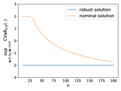
(a)

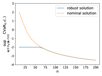
(b)

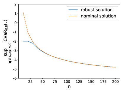
(c)

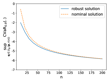
(d)

We note that $\pi(d_{i},y)$ is concave in $y$ since it is a sum of concave piecewise-linear functions in $y$ for all $i$. Assume that the demand $d_{i}\in\{4,8,10\}$ corresponding to low demand, medium demand, and high demand, with nominal probabilities $\mathbf{p}=\{0.375,0.375,0.25\}$. We assume that the number of items ordered will not exceed the maximum demand, i.e., $y\leq 10$. Furthermore, we set the parameter values $c=4,v=6,s=2,l=4$.

We solve both the robust problem (P) and the nominal problem $\eqref{P-Nom}$, where $y$ is the decision variable subject to the constraint $0\leq y\leq 10$, $d$ is the uncertain parameter, and $\pi(d,y)$ is the random objective function. We choose $\mathrm{CVaR}_{1-\alpha_{0}}$ (see (6)) to be our rank-dependent evaluation $\rho_{u,h,\mathbf{q}}$. This corresponds to a piecewise-linear distortion function $h(p)=\min\{p/(1-\alpha_{0}),1\}$ and a linear utility function $u(x)=x$. For the robust problem (P), we choose the KL-divergence function $\phi(t)=t\log(t)-t+1$, and set the radius of the divergence set $\mathcal{D}_{\phi}(\mathbf{p},r)$ to be $r=\chi^{2}_{2,0.95}/(2n)$ as in (10), where $n$ is a fictitious sample size that we assume that $\mathbf{p}$ is estimated from.

Since the number of realizations of the uncertain parameter $d$ is merely 3, we can simply apply Theorem 2 to solve both the reformulated nominal and robust problems (P-ref) and (P-Nom-ref), without using any approximations to reduce the number of constraints. We then perform the following experiment: For each $\alpha_{0}$, we first obtain a nominal solution by solving (P-Nom). Then, for each radius $r(n)=\chi^{2}_{2,0.95}/(2n)$, we solve (P) to obtain a robust solution. To compare the robust solution with the nominal solution, we calculate their worst-case evaluation $\sup_{\mathbf{q}\in\mathcal{D}_{\phi}(\mathbf{p},r(n))}\mathrm{CVaR}_{1-\alpha_{0}}(.)$ under the radius $r(n)$. This is repeated for a range of $n=10,20,\ldots,200$, and $\alpha_{0}=0.4,0.3,0.2,0.1$. As $n$ increases, the $\phi$-divergence radius $r$ decreases, and thus there is less ambiguity. Therefore, we expect the difference between the worst-case evaluations of both solutions to decrease as $n$ increases. We also expect a decrease of the value of the worst-case evaluation as $\alpha_{0}$ decreases, since the $\mathrm{CVaR}_{1-\alpha_{0}}$ risk measure has a lower value with a smaller $\alpha_{0}$.

The results are displayed in Figure 1, which agree with our expectations. Furthermore, we see that for lower values of $\alpha_{0}$, the difference between the worst-case evaluations of both solutions is already small for low sample size of $n$. We also observe a constant worst-case evaluation of the robust solution at $-2$. This is the largest value that the robust rank-dependent evaluation can attain for a solution $y^{*}=7$. This conservativeness happens when $n$ is sufficiently small.

To further illustrate the difference between the robust and nominal solutions, we use the Hit-and-Run algorithm (see Electronic Companion EC.7 for further details) to sample $5\mathord{,}000$ probability vectors $\mathbf{q}$ from the KL-divergence uncertainty set for $n=50$. For each sampled vector $\mathbf{q}$, we calculate the $\mathrm{CVaR}_{1-\alpha_{0}}$ evaluation under the sampled distribution vector $\mathbf{q}$ for $\alpha_{0}=0.4$.

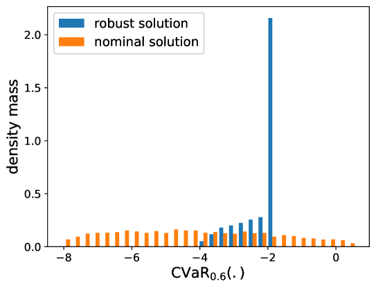
Figure 2: Comparison between the robust and nominal solutions under variation of the nominal probability $\mathbf{p}$. For each sampled probability $\mathbf{q}$, the $\mathrm{CVaR}_{1-\alpha_{0}}(.)$ evaluation with $\alpha_{0}=0.4$ of both solutions are computed.

As shown in Figure 2, the evaluation of the nominal solution exhibits a large variance. It also exceeds the largest evaluation of the robust solution. On the other hand, the robust solution shows less variance and is concentrated at the value $-2$, which as mentioned before, is the most conservative evaluation that the robust optimal solution can attain.

7.2 Robust Multi-Item Newsvendor

We also examine the multi-item newsvendor problem, where each item has its own uncertain demand. Let $d^{(j)}_{i}$ be the $i$-th realization of the $j$-th item’s demand, $i=1,2,3$. We assume that the demand takes on the same possible values for all items, i.e., $d^{(j)}_{i}\in\{4,8,10\}$ for all $j$. We take $j=1,2,3$ and consider the sum of the individual profit functions

$$\pi_{\mathrm{tot}}(\mathbf{d},\mathbf{y})=\pi_{1}(d^{(1)},y_{1})+\pi_{2}(d^{(2)},y_{2})+\pi_{3}(d^{(3)},y_{3}),$$ (58)

where

$$\pi_{j}(d^{(j)},y_{j}) =v_{j}\min\{d^{(j)},y_{j}\}+s_{j}(y_{j}-d^{(j)})_{+}-l_{j}(d^{(j)}-y_{j})_{+}-c_{j}y_{j},$$ (59)

with $v_{j},s_{j},l_{j},c_{j}$ the parameters corresponding to item $j$. Since each realization of $d^{(j)}$ contributes to a possible realization of $\pi_{\mathrm{tot}}(\mathbf{y},\mathbf{d})$, there are in total $m=3^{3}=27$ possible realizations. We solve again the problems (P) and (P-Nom) with the same set-ups as in the single-item problem. Since the $\mathrm{CVaR}_{1-\alpha_{0}}$ risk measure has a piecewise-linear distortion function, we can apply Theorem 37 to solve (P-ref) and (P-Nom-ref). We take the nominal probability $\mathbf{p}\in\mathbb{R}^{27}$ to be the probability of each combination of realizations of $(d^{(1)},d^{(2)},d^{(3)})$, which is the product of the probabilities $\mathbf{p}^{(1)},\mathbf{p}^{(2)},\mathbf{p}^{(3)}$ of each individual realization. The parameters we used for our example are taken from Ben-Tal et al., (2013) and are given in Table 1.

Table 1: Parameters used in the multi-item newsvendor problem.

$\mathrm{Item}(j)$	$c$	$v$	$s$	$l$	$p^{(j)}_{1}$	$p^{(j)}_{2}$	$p^{(j)}_{3}$
1	4	6	2	4	0.375	0.375	0.25
2	5	8	2.5	3	0.25	0.25	0.5
3	4	5	1.5	4	0.127	0.786	0.087

Similar to the single-item problem, we investigate the difference in the worst-case risk evaluation of the robust and nominal solutions, for a range of $n$ and $\alpha_{0}$. We choose $\alpha_{0}=0.4,0.3$ to compare the result with the single-item problem and $\alpha_{0}=0.9,0.8$ to explore the higher values of $\alpha_{0}$. As shown in Figure 3, we see that in the multi-item problem, the worst-case risk evaluation value is much lower than the single-item problem. The pattern is similar to the single-item case, namely that for relatively lower $\alpha_{0}$, the difference in worst-case risk evaluation values between the robust solution and the nominal solution is smaller compared to the relatively higher $\alpha_{0}$. The same holds as the sample size $n$ increases.

Figure 3: Multi-item newsvendor problem: The worst-case evaluation $\sup_{\mathbf{q}\in\mathcal{D}_{\phi}(\mathbf{p},r(n))}\mathrm{CVaR}_{1-\alpha_{0}}(.)$ calculated for the robust and nominal solutions, for a range of values of $r(n)=\chi^{2}_{2,0.95}/(2n)$ and $\alpha_{0}=0.9,0.8,0.4,0.3$.

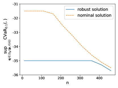
(a)

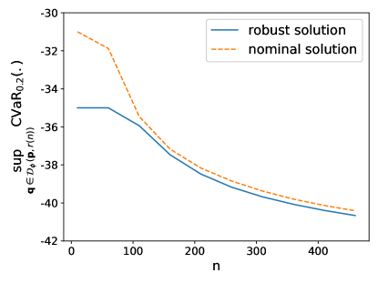
(b)

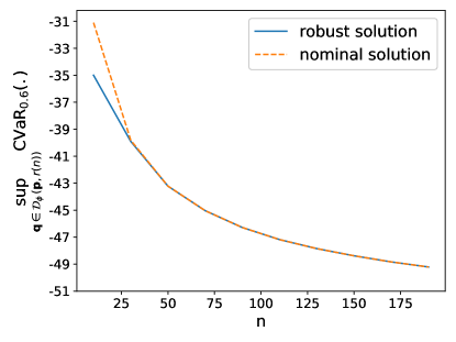
(c)

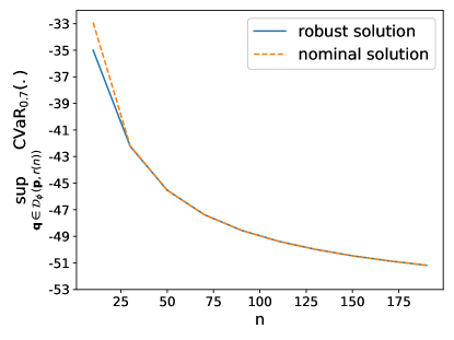
(d)

7.3 Robust Portfolio Choice

In this subsection, we investigate the performance of the cutting-plane algorithm and the piecewise-linear approximation method described in Algorithms 1 and 2, by studying robust portfolio optimization problems. We use the returns of the six portfolios formed on size and book-to-market ratio (2$\times$3) obtained from Kenneth French’s data library. We choose monthly returns from January 1984 to January 2014. This gives us a total of $m=360$ return realizations for each of the six portfolios. The nominal probability $\mathbf{p}$ is set to be the empirical distribution with $p_{i}=\frac{1}{360}$. We use the modified chi-squared divergence function $\phi(x)=(x-1)^{2}$, with radius $r=\frac{1}{n}\chi^{2}_{359,0.95}$. We choose the distortion function $h(p)=1-(1-p)^{2}$, motivated by two decision-theoretic papers: Eeckhoudt et al., (2020) and Eeckhoudt and Laeven, (2021). Furthermore, we choose the exponential utility function $u(x)=1-e^{-x/\lambda}$ with $\lambda=10$.

We solve the following robust and nominal portfolio optimization problems:

$$\min_{\mathbf{a}\in\mathcal{A}} \leavevmode\nobreak\ \rho_{u,h,\mathbf{p}}(1+\mathbf{a}^{T}\mathbf{r})$$ (60)

$$\min_{\mathbf{a}\in\mathcal{A}} \sup_{\mathbf{q}\in\mathcal{D}_{\phi}(\mathbf{p},r)}\rho_{u,h,\mathbf{q}}(1+\mathbf{a}^{T}\mathbf{r}),$$ (61)

where $1+\mathbf{a}^{T}\mathbf{r}$ is the total wealth after one period, evaluated under the rank-dependent model. The decision variable $\mathbf{a}\in\mathbb{R}^{6}$ is subject to the constraints $\mathcal{A}=\{\mathbf{a}\in\mathbb{R}^{6}\leavevmode\nobreak\ |\leavevmode\nobreak\ \sum^{6}_{j=1}a_{j}=1,a_{j}\geq 0\}$. We denote by $\mathbf{r}$ the uncertain return of the six portfolios with realizations $\mathbf{r}_{1},\ldots,\mathbf{r}_{360}$.

We solve problems (61) and (60) with the cutting-plane method described in Algorithm 1, and compare its performance to the piecewise-linear method described in Algorithm 2. As shown in Table 2, both algorithms yield a very small gap between the upper and lower bounds they provide. The piecewise-linear approximation method is typically faster, but this is not surprising, since the cutting-plane method is a more general method and utilizes less structure of the problems at hand.

Table 2: Algorithms 1 and 2 applied to the robust problem (61) and the nominal problem (60). The tolerance parameters of both methods are set to $\epsilon_{\mathrm{tol}}=0.0001$ and $\epsilon=0.001$. For Panel B, the optimal portfolio in the last column is obtained by taking the lower bound solution.

Panel A: The cutting-plane method
Problem	Lower Bound	Upper Bound	# Cuts	Run Time	Optimal Portfolio
Robust	-0.08953	-0.08948	5	54 sec	$(0,0,0,0.251,0.749,0)$
Nominal	-0.09403	-0.09397	5	22 sec	$(0,0,0.144,0.385,0.472,0)$

(a)

Panel B: Piecewise-linear approximation
Problem	Lower Bound	Upper Bound	Total Run Time	Optimal Portfolio (lb)
Robust	-0.08951	-0.08948	14 sec	$(0,0,0,0.380,0.620,0)$
Nominal	-0.09401	-0.09398	7 sec	$(0,0.0859,0.207,0.131,0.576,0)$

(b)

Additionally, for the two solutions obtained from the cutting-plane algorithm, we calculate the worst-case rank-dependent evaluation of the nominal solution, which is equal to $-0.08938$. We also calculate the evaluation of the robust solution under the nominal distribution $\mathbf{p}$, which is equal to $-0.09395$. As we can see, the worst-case evaluation of the nominal solution is not much larger than that of the robust solution, suggesting that the nominal solution is already “near-optimal” for the robust problem (61). Similarly, the robust solution is also “near-optimal” for the nominal problem (60). It seems that when the dimension $m$ of the state space is large, the robust and nominal problems do not yield very different solutions.

7.3.1 Robust Portfolio with Inverse $S$-shaped Distortion Function

In this subsection, we investigate portfolio optimization problems (60) and (61), where $h$ is an inverse $S$-shaped distortion function. In particular, we examine Prelec’s distortion function (Prelec,, 1998):

$$h(p)=1-\exp(-(-\log(1-p))^{\alpha}).$$ (62)

We examine three values of $\alpha=0.6,0.65,0.75$, where $\alpha=0.65$ is the benchmark value that is most consistent with common empirical findings. To obtain an upper and a lower bound on the problems (60) and (61), we approximate the Prelec’s function from above and from below, using piecewise-linear functions consisting of 13 pieces. The approximation procedure is carried out by applying the method described in Section 5.2 separately to the concave and convex parts of the Prelec’s function, where we minimized the number of linear pieces under certain approximation error . The shape of the Prelec’s functions with the chosen values of $\alpha$, and their respective upper and lower approximations, are plotted in Figure 4.

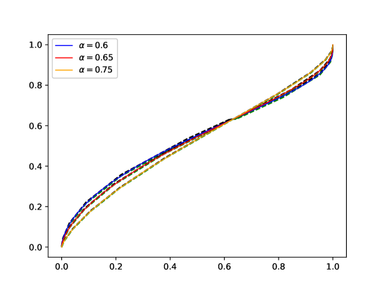
Figure 4: Upper and lower piecewise-linear approximations (displayed in dashed lines) of the Prelec’s distortion functions (62) for $\alpha=0.6,0.65,0.75$.

We generate 100 return data points for 5 assets using the same numerical scheme as in Esfahani and Kuhn, (2018), where the returns for each asset $j\in\{1,\ldots,5\}$ are composed of two factors:

$$r_{j}=\psi+\gamma_{j},$$

where we have a systematic risk factor $\psi\sim N(0,0.02)$ and an idiosyncratic risk factor $\gamma_{j}\sim N(0.03j,0.25j)$, for the $j$-th asset. Here, $N(\mu,\sigma^{2})$ denotes the Gaussian distribution. By construction, the asset with a higher index $j$ has a higher expected return and variance.

We obtain lower and upper bounds on the nominal problem (60) by implementing the constraints (53) respectively for the lower and upper linear approximation of $h$ in the Gurobi (Version 11.0.3) solver. A lower bound for the robust problem (61) is obtained by calculating the lower bound obtained through the cutting-plane method described in Algorithm 3 (where we set $\epsilon_{\mathrm{tol}}=0.001$), while also using a lower approximation of $h$. Then, with the solution obtained from the cutting-plane method, we determine an upper bound on (61) by calculating its worst-case evaluation using the SOS2-constraints as in (55). For the robust problem, we investigate both the total variation divergence $\phi(t)=|t-1|$ and the modified chi-squared divergence $\phi(t)=(t-1)^{2}$. We choose the radius for both robust problems to be $r=\frac{1}{m}\chi^{2}_{m-1,0.95}$, where $m=100$. The results are shown in Tables 3. As we can see, Gurobi solves the nominal problem (60) efficiently, but the robust problem (61) takes longer time (and considerably longer if $\phi$ is quadratic). Moreover, we observe tight upper and lower bounds, where most gap values are around $0.002$.

Table 3: Upper and lower bounds (UB and LB) obtained for the nominal problem (60) and the robust problem (61), where $\phi(t)\in\{|t-1|,(t-1)^{2}\}$, and $h$ is a Prelec’s distortion function with $\alpha\in\{0.6,0.65,0.75\}$, see Figure 4. The number of return realizations is $m=100$.

Panel A: Solutions Nominal Problem
$\alpha$	LB	UB	Run Time (LB)	Run Time (UB)
0.6	-1.146	-1.142	0.77 sec	0.76 sec
0.65	-1.148	-1.146	0.88 sec	2.12 sec
0.75	-1.153	-1.152	0.45 sec	1.00 sec

(a)

Panel B: Solutions Robust Problem with $\phi(t)=|t-1|$
$\alpha$	LB	UB	# Cuts	Run Time (LB)	Run Time (UB)
0.6	-1.042	-1.040	9	227 sec	1.29 sec
0.65	-1.041	-1.039	9	209 sec	1.03 sec
0.75	-1.039	-1.038	9	127 sec	1.21sec

(b)

Panel C: Solutions Robust Problem with $\phi(t)=(t-1)^{2}$
$\alpha$	LB	UB	# Cuts	Run Time (LB)	Run Time (UB)
0.6	-1.059	-1.060	9	3700 sec	334 sec
0.65	-1.062	-1.060	10	3825 sec	521 sec
0.75	-1.062	-1.061	11	4262 sec	162 sec

(c)

8 Concluding Remarks

In this paper, we have shown that non-robust and robust optimization problems involving rank-dependent models can be reformulated into rank-independent, tractable optimization problems. When the distortion function is concave, we have demonstrated that this reformulation admits a conic representation, which we have explicitly derived for canonical distortion and divergence functions. Whereas the number of constraints in the reformulation increases exponentially with the dimension of the underlying probability space, we have developed two algorithms to circumvent this curse of dimensionality. We have established that the upper and lower bounds the algorithms generate converge to the optimal objective value. Finally, we have illustrated the good performance of our methods in two examples involving concave as well as inverse-$S$-shaped distortion functions, yielding very tight upper and lower bounds.

As a direction for future research, one can investigate whether the approach developed in this paper can be extended to encompass robust optimization problems with general law-invariant convex risk measures, which also admit a dual representation.

Appendix

Appendix EC.1 Proofs

Proof of Theorem 1.

Let $\mathbf{q}$ be any probability vector and denote $\mathbb{Q}$ its corresponding probability measure on the sigma-algebra $2^{|\Omega|}$ (the set of all subsets of $\Omega$). The set function $h\circ\mathbb{Q}$, is by Example 2.1, Denneberg, (1994), a monotone, submodular set function. It then follows from Proposition 10.3 of Denneberg, (1994) that for any random variable $X$, we have

$$\rho_{u,h,\mathbf{q}}(X)=\sup_{\mathbf{\bar{q}}\in M_{h}(\mathbf{q})}\mathbb{E}_{\mathbf{\bar{q}}}[-u(X)].$$

Hence, we have that

$$\sup_{\mathbf{q}\in\mathcal{D}_{\phi}(\mathbf{p},r)}\rho_{u,h,\mathbf{q}}(f(\mathbf{a},\mathbf{X})) =\sup_{\mathbf{q}\in\mathcal{D}_{\phi}(\mathbf{p},r)}\sup_{\mathbf{\bar{q}}\in M_{h}(\mathbf{q})}\mathbb{E}_{\mathbf{\bar{q}}}[-u(f(\mathbf{a},\mathbf{X}))]$$

$$=\sup_{(\mathbf{q},\bar{\mathbf{q}})\in\mathcal{U}_{\phi,h}(\mathbf{p})}-\sum^{m}_{i=1}\bar{q}_{i}u(f(\mathbf{a},\mathbf{x}_{i})).$$

∎

Proof of Theorem 2.

Suppose a pair of $(\mathbf{a},c)\in\mathbb{R}^{n_{a}+1}$ satisfies

$$\sup_{(\mathbf{q},\mathbf{\bar{q}})\in\mathcal{U}_{\phi,h}(\mathbf{p})}-\sum^{m}_{i=1}\bar{q}_{i}u(f(\mathbf{a},\mathbf{x}_{i}))\leq c.$$ (EC.1)

Then, the left-hand side of (EC.1) is a maximization problem upper bounded by $c<\infty$. Moreover, the set $\mathcal{U}_{\phi,h}(\mathbf{p})$ contains $(\mathbf{p},\mathbf{p})$ as a slater point, since $\phi(1)=0<r$ and $h(\sum_{k\in I_{j}}p_{k})>\sum_{k\in I_{j}}p_{k}$ for all subsets $I_{j}\subset[m]$ that is not $\emptyset$ and $[m]$. Therefore, strong duality holds, and we examine the Lagrangian function:

$$L(\mathbf{a},\mathbf{q},\bar{\mathbf{q}},\alpha,\beta,(\lambda_{j})_{j},\gamma)$$

$$=-\sum^{m}_{i=1}\bar{q}_{i}u(f(\mathbf{a},\mathbf{x}_{i}))-\alpha\left(\sum^{m}_{i=1}q_{i}-1\right)-\beta\left(\sum^{m}_{i=1}\bar{q}_{i}-1\right)-\sum^{2^{m}-2}_{j=1}\lambda_{j}\left(\sum_{k\in I_{j}}\bar{q}_{k}-h\left(\sum_{k\in I_{j}}q_{k}\right)\right)$$

$$\leavevmode\nobreak\ \leavevmode\nobreak\ \leavevmode\nobreak\ \leavevmode\nobreak\ \leavevmode\nobreak\ \leavevmode\nobreak\ -\gamma\left(\sum^{m}_{i=1}p_{i}\phi\left(\frac{q_{i}}{p_{i}}\right)-r\right)$$

$$=\alpha+\beta+\gamma r+\sum^{m}_{i=1}-(u(f(\mathbf{a},\mathbf{x}_{i}))+\beta)\bar{q}_{i}-\sum^{2^{m}-2}_{j=1}\lambda_{j}\sum_{k\in I_{j}}\bar{q}_{k}+\sum^{m}_{i=1}-\alpha q_{i}-\gamma\left(\sum^{m}_{i=1}p_{i}\phi\left(\frac{q_{i}}{p_{i}}\right)\right)$$

$$\leavevmode\nobreak\ \leavevmode\nobreak\ \leavevmode\nobreak\ \leavevmode\nobreak\ \leavevmode\nobreak\ \leavevmode\nobreak\ -\sum^{2^{m}-2}_{j=1}-\lambda_{j}h\left(\sum_{k\in I_{j}}q_{k}\right),$$

for $\alpha,\beta\in\mathbb{R}$ and $\lambda_{j},\gamma\geq 0$. We examine $\sup_{\mathbf{q},\mathbf{\bar{q}}\geq 0}L(\mathbf{a},\mathbf{q},\mathbf{\bar{q}},\alpha,\beta,(\lambda_{j})_{j},\gamma)$, which excluding the constant $\alpha+\beta+\gamma r$ is equal to:

$$\sup_{\mathbf{q},\bar{\mathbf{q}}\geq 0}\sum^{m}_{i=1}-(u(f(\mathbf{a},\mathbf{x}_{i}))+\beta)\bar{q}_{i}-\sum^{2^{m}-2}_{j=1}\lambda_{j}\sum_{k\in I_{j}}\bar{q}_{k}+\sum^{m}_{i=1}-\alpha q_{i}-\gamma p_{i}\phi\left(\frac{q_{i}}{p_{i}}\right)-\sum^{2^{m}-2}_{j=1}\lambda_{j}(-h)\left(\sum_{k\in I_{j}}q_{k}\right)$$

$$=\sup_{\bar{\mathbf{q}}\geq 0}\sum^{m}_{i=1}-(u(f(\mathbf{a},\mathbf{x}_{i}))+\beta)\bar{q}_{i}-\sum^{2^{m}-2}_{j=1}\lambda_{j}\sum_{k\in I_{j}}\bar{q}_{k}+\sup_{\mathbf{q}\geq 0}\sum^{m}_{i=1}-\alpha q_{i}-\gamma p_{i}\phi\left(\frac{q_{i}}{p_{i}}\right)-\sum^{2^{m}-2}_{j=1}\lambda_{j}(-h)\left(\sum_{k\in I_{j}}q_{k}\right).$$

We examine both supremum terms separately. The first supremum gives:

$$\sup_{\bar{\mathbf{q}}\geq 0}\sum^{m}_{i=1}-(u(f(\mathbf{a},\mathbf{x}_{i}))+\beta)\bar{q}_{i}-\sum^{2^{m}-2}_{j=1}\lambda_{j}\sum_{k\in I_{j}}\bar{q}_{k} =\sup_{\bar{\mathbf{q}}\geq 0}\sum^{m}_{i=1}-\left(u(f(\mathbf{a},\mathbf{x}_{i}))+\beta+\sum_{j:i\in I_{j}}\lambda_{j}\right)\bar{q}_{i}$$

$$=\begin{cases}0&\text{if}\leavevmode\nobreak\ u(f(\mathbf{a},\mathbf{x}_{i}))+\beta+\sum_{j:i\in I_{j}}\lambda_{j}\geq 0,\leavevmode\nobreak\ \forall i\\ \infty&\text{else}.\end{cases}$$

The second supremum gives:

$$\sup_{\mathbf{q}\geq 0}\sum^{m}_{i=1}-\alpha q_{i}-\gamma p_{i}\phi\left(\frac{q_{i}}{p_{i}}\right)-\sum^{2^{m}-2}_{j=1}\lambda_{j}(-h)\left(\sum_{k\in I_{j}}q_{k}\right)$$

$$=\sup_{\begin{subarray}{c}\mathbf{q}\geq\mathbf{0}\\ w_{1},\ldots,w_{2^{m}-2}\geq 0\end{subarray}}\left\{\sum^{m}_{i=1}-\alpha q_{i}-\gamma p_{i}\phi\left(\frac{q_{i}}{p_{i}}\right)-\sum^{2^{m}-2}_{j=1}\lambda_{j}(-h)(w_{j})\leavevmode\nobreak\ \middle|\leavevmode\nobreak\ w_{j}=\sum_{k\in I_{j}}q_{k}\right\}$$

$$=\inf_{\nu_{1},\ldots,\nu_{2^{m}-2}}\sup_{\begin{subarray}{c}\mathbf{q}\geq\mathbf{0}\\ w_{1},\ldots,w_{2^{m}-2}\geq 0\end{subarray}}\sum^{m}_{i=1}-\alpha q_{i}-\gamma p_{i}\phi\left(\frac{q_{i}}{p_{i}}\right)-\sum^{2^{m}-2}_{j=1}\lambda_{j}(-h)(w_{j})-\sum^{2^{m}-2}_{j=1}\nu_{j}\left(w_{j}-\sum_{k\in I_{j}}q_{k}\right)$$

$$=\inf_{\nu_{1},\ldots,\nu_{2^{m}-2}}\sup_{\mathbf{q}\geq 0}\sum^{m}_{i=1}\left(-\alpha+\sum_{j:i\in I_{j}}\nu_{j}\right)q_{i}-\gamma p_{i}\phi\left(\frac{q_{i}}{p_{i}}\right)+\sup_{w_{1},\ldots,w_{2^{m}-2}\geq 0}\sum^{2^{m}-2}_{j=1}-\nu_{j}w_{j}-\lambda_{j}(-h)(w_{j})$$

$$=\inf_{\nu_{1},\ldots,\nu_{2^{m}-2}}\sum^{m}_{i=1}p_{i}\left(\sup_{t\geq 0}\left(-\alpha+\sum_{j:i\in I_{j}}\nu_{j}\right)t-\gamma\phi(t)\right)+\sum^{2^{m}-2}_{j=1}\lambda_{j}(-h)^{*}\left(\frac{-\nu_{j}}{\lambda_{j}}\right)$$

$$=\inf_{\nu_{1},\ldots,\nu_{2^{m}-2}}\sum^{m}_{i=1}p_{i}\gamma\phi^{*}\left(\frac{-\alpha+\sum_{j:i\in I_{j}}\nu_{j}}{\gamma}\right)+\sum^{2^{m}-2}_{j=1}\lambda_{j}(-h)^{*}\left(\frac{-\nu_{j}}{\lambda_{j}}\right),$$

where $\phi^{*}$ and $(-h)^{*}$ are the conjugates of $\phi$ and $-h$. Therefore, strong duality implies that a pair $(\mathbf{a},c)$ satisfies

$$\sup_{(\mathbf{q},\mathbf{\bar{q}})\in\mathcal{U}_{\phi,h}(\mathbf{p})}-\sum_{i}\bar{q}_{i}u(f(\mathbf{a},\mathbf{x}_{i}))\leq c$$

if and only if

$$\inf_{\begin{subarray}{c}\alpha,\beta,\nu_{j}\in\mathbb{R}\\ \lambda_{j},\gamma\geq 0\end{subarray}} \alpha+\beta+\gamma r+\sum^{m}_{i=1}p_{i}\gamma\phi^{*}\left(\frac{-\alpha+\sum_{j:i\in I_{j}}\nu_{j}}{\gamma}\right)+\sum^{2^{m}-2}_{j=1}\lambda_{j}(-h)^{*}\left(\frac{-\nu_{j}}{\lambda_{j}}\right)\leq c$$

subject to $$\leavevmode\nobreak\ -u(f(\mathbf{a},\mathbf{x}_{i}))-\beta-\sum_{j:i\in I_{j}}\lambda_{j}\leq 0,\leavevmode\nobreak\ \forall i\in[m].$$

Since the infimum is attained due to the strong duality theorem and the boundedness of the primal problem (EC.1), we may remove the infimum sign and obtain that the above holds if and only if there exists $\lambda_{j},\gamma\geq 0,\alpha,\beta,\nu_{j}\in\mathbb{R}$ such that

$$\begin{cases}\alpha+\beta+\gamma r+\sum^{m}_{i=1}p_{i}\gamma\phi^{*}\left(\frac{-\alpha+\sum_{j:i\in I_{j}}\nu_{j}}{\gamma}\right)+\sum^{2^{m}-2}_{j=1}\lambda_{j}(-h)^{*}\left(\frac{-\nu_{j}}{\lambda_{j}}\right)\leq c\\ -u(f(\mathbf{a},\mathbf{x}_{i}))-\beta-\sum_{j:i\in I_{j}}\lambda_{j}\leq 0,\leavevmode\nobreak\ \forall i\\ \lambda_{j},\gamma\geq 0\\ \alpha,\beta,\nu_{j}\in\mathbb{R},\leavevmode\nobreak\ j=1,\ldots,M.\end{cases}$$

For the nominal problem, the Lagrangian function would be

$$L(\mathbf{a},\bar{\mathbf{q}},\beta,(\lambda_{j})_{j}) =-\sum^{m}_{i=1}\bar{q}_{i}u(f(\mathbf{a},\mathbf{x}_{i}))-\beta\left(\sum^{m}_{i=1}\bar{q}_{i}-1\right)-\sum^{2^{m}-2}_{j=1}\lambda_{j}\left(\sum_{k\in I_{j}}\bar{q}_{k}-h\left(\sum_{k\in I_{j}}p_{k}\right)\right)$$

$$=\beta+\sum^{2^{m}-2}_{j=1}\lambda_{j}h\left(\sum_{k\in I_{j}}p_{k}\right)+\sum^{m}_{j=1}\bar{q}_{i}\left(-u(f(\mathbf{a},\mathbf{x}_{i}))-\beta-\sum_{j:i\in I_{j}}\lambda_{j}\right).$$

Hence, we have

$$\sup_{\bar{\mathbf{q}}\in M_{h}(\mathbf{p})}\sum^{m}_{i=1}-\bar{q}_{i}u(f(\mathbf{a},\mathbf{x}_{i}))$$

$$=\inf_{\beta\in\mathbb{R},\lambda_{j}\geq 0}\sup_{\bar{\mathbf{q}}\geq\mathbf{0}}L(\mathbf{a},\bar{\mathbf{q}},\beta,(\lambda_{j})_{j})$$

$$=\inf_{\beta\in\mathbb{R},\lambda_{j}\geq 0}\left\{\beta+\sum^{2^{m}-2}_{j=1}\lambda_{j}h\left(\sum_{k\in I_{j}}p_{k}\right)\leavevmode\nobreak\ \middle|\leavevmode\nobreak\ -u(f(\mathbf{a},\mathbf{x}_{i}))-\beta-\sum_{j:i\in I_{j}}\lambda_{j}\leq 0,\leavevmode\nobreak\ \forall i\in[m]\right\},$$

where the above strong duality holds since we are solving a linear programming problem. Therefore, we have that $\sup_{\bar{\mathbf{q}}\in M_{h}(\mathbf{p})}\sum^{m}_{i=1}-\bar{q}_{i}u(f(\mathbf{a},\mathbf{x}_{i}))\leq c$, if and only if there exists $\beta\in\mathbb{R},(\lambda_{j})_{j}\geq 0$ such that

$$\begin{cases}\beta+\sum^{2^{m}-2}_{j=1}\lambda_{j}h\left(\sum_{k\in I_{j}}p_{k}\right)\leq c\\ -u(f(\mathbf{a},\mathbf{x}_{i}))-\beta-\sum_{j:i\in I_{j}}\lambda_{j}\leq 0,\leavevmode\nobreak\ \forall i\in[m]\\ \beta\in\mathbb{R},\lambda_{j}\geq 0,\leavevmode\nobreak\ \forall j=1,\ldots,2^{m}-2.\end{cases}$$

∎

Proof of Lemma 1.

The proof is identical to Ben-Tal and Nemirovski, (2019), except that we replace the quadratic cone with a general cone. We have,

$$\mathrm{Epi}(f^{*})=\{(\mathbf{y},s):\mathbf{y}^{T}\mathbf{x}-f(\mathbf{x})\leq s,\forall\mathbf{x}\} =\{(\mathbf{y},s):\mathbf{y}^{T}\mathbf{x}-t\leq s,\forall(\mathbf{x},t)\in\mathrm{Epi}(f)\}.$$

Therefore, we have $(\mathbf{y},s)\in\mathrm{Epi}(f^{*})$ if and only if

$$\min_{\mathbf{x},t,\mathbf{w}}\{-\mathbf{y}^{T}\mathbf{x}+t:\mathbf{A}\mathbf{x}+t\mathbf{v}+\mathbf{B}\mathbf{w}+\mathbf{b}\succeq_{\mathbf{K}}\mathbf{0}\}\geq-s.$$

This minimization problem is strictly feasible and bounded from below. Hence, the conic duality theorem (see Ben-Tal and Nemirovski,, 2019) implies that it is equal to

$$\max_{\boldsymbol{\xi}}\{-\mathbf{b}^{T}\boldsymbol{\xi}:\mathbf{A}^{T}\boldsymbol{\xi}=-\mathbf{y},\mathbf{B}^{T}\boldsymbol{\xi}=\mathbf{0},\mathbf{v}^{T}\boldsymbol{\xi}=1,\boldsymbol{\xi}\in\mathbf{K}^{*}\}.$$

Therefore, we have

$$\mathrm{Epi}(f^{*})=\{(\mathbf{y},s):\exists\leavevmode\nobreak\ \boldsymbol{\xi}\in\mathbf{K}^{*}:\mathbf{A}^{T}\boldsymbol{\xi}=-\mathbf{y},\mathbf{B}^{T}\boldsymbol{\xi}=\mathbf{0},\mathbf{v}^{T}\boldsymbol{\xi}=1,s\geq\mathbf{b}^{T}\boldsymbol{\xi}\}.$$

∎

Proof of Lemma 2.

Following Ben-Tal and Nemirovski, (2019), we have

$$\mathrm{Epi}(\tilde{f})=\left\{(\mathbf{x},\lambda,t):\lambda f\left(\frac{\mathbf{x}}{\lambda}\right)\leq t\right\} =\left\{(\mathbf{x},\lambda,t):\left(\frac{\mathbf{x}}{\lambda},\frac{t}{\lambda}\right)\in\mathrm{Epi}(f)\right\}$$

$$=\{(\mathbf{x},\lambda,t):\exists\leavevmode\nobreak\ \mathbf{w}\in\mathbb{R}^{k}:\mathbf{A}(\mathbf{x}/\lambda,\mathbf{w},t/\lambda)^{T}-b\succeq_{\mathbf{K}}\mathbf{0}\}$$

$$=\{(\mathbf{x},\lambda,t):\exists\leavevmode\nobreak\ \tilde{\mathbf{w}}\in\mathbb{R}^{k}:\mathbf{A}(\mathbf{x}/\lambda,\tilde{\mathbf{w}}/\lambda,t/\lambda)^{T}-b\succeq_{\mathbf{K}}\mathbf{0}\}$$

$$=\{(\mathbf{x},\lambda,t):\exists\leavevmode\nobreak\ \tilde{\mathbf{w}}\in\mathbb{R}^{k}:\mathbf{A}(\mathbf{x},\tilde{\mathbf{w}},t)^{T}-\lambda b\succeq_{\mathbf{K}}\mathbf{0}\}$$

$$=\{(\mathbf{x},\lambda,t):\exists\leavevmode\nobreak\ \tilde{\mathbf{w}}\in\mathbb{R}^{k}:[\mathbf{A},-b](\mathbf{x},\tilde{\mathbf{w}},t,\lambda)^{T}\succeq_{\mathbf{K}}\mathbf{0}\}.$$

∎

Proof of Lemma 3.

By definition, $\mathbf{q}^{*}\in\mathcal{D}_{\phi}(\mathbf{p},r)$. Hence, we only need to show that $\bar{\mathbf{q}}^{*}\in M_{h}(\mathbf{q}^{*})$. Using Lemma 4.98 of Föllmer and Schied, (2016), we have that $\rho_{u,h,\mathbf{q}^{*}}(X)\geq\mathbb{E}_{\bar{\mathbf{q}}^{*}}[-X]$ for all random variables $X$ (where $\rho_{u,h,\mathbf{q}^{*}}(X)$ is as defined in (4) with measure $\mathbb{Q}=\mathbf{q}$). In particular, this holds for all $X=-\mathbbm{1}_{A}$, for any measurable set $A\subset\Omega$. Hence, $(\mathbf{q}^{*},\bar{\mathbf{q}}^{*})\in\mathcal{U}_{\phi,h}(\mathbf{p})$. ∎

Proof of Theorem 3.

The proof follows the idea presented in Mutapcic and Boyd, (2009). First, we have, for any $\mathbf{a}^{1},\mathbf{a}^{2}\in\mathcal{A}$, that the following inequality holds:

$$\begin{split}\left|\sum_{i=1}^{m}\bar{q}_{i}u(f(\mathbf{a}^{2},\mathbf{x}_{i}))-\sum_{i=1}^{m}\bar{q}_{i}u(f(\mathbf{a}^{1},\mathbf{x}_{i}))\right|&\leq\|\mathbf{\bar{q}}\|_{2}\|(u(f(\mathbf{a}^{2},\mathbf{x}_{i}))-u(f(\mathbf{a}^{1},\mathbf{x}_{i})))^{m}_{i=1}\|_{2}\\ &\leq\|\mathbf{\bar{q}}\|_{1}\|(u(f(\mathbf{a}^{2},\mathbf{x}_{i}))-u(f(\mathbf{a}^{1},\mathbf{x}_{i})))^{m}_{i=1}\|_{2}\\ &=\|(u(f(\mathbf{a}^{2},\mathbf{x}_{i}))-u(f(\mathbf{a}^{1},\mathbf{x}_{i})))^{m}_{i=1}\|_{2},\end{split}$$ (EC.2)

where the first inequality follows from Cauchy-Schwarz. The second inequality follows from $\|\bar{\mathbf{q}}\|_{2}\leq\|\bar{\mathbf{q}}\|_{1}$ for $\bar{\mathbf{q}}$ a probability vector, since $\bar{q}_{k}^{2}\leq\bar{q}_{k}$ for $|\bar{q}_{k}|\leq 1$.

Suppose now that the cutting-plane method has not terminated at the $t$-th iteration, i.e., the optimal solution and objective value $(\mathbf{a}_{t},c_{t})$ violate the $\epsilon_{\mathrm{tol}}$-feasibility condition at step 4 of Algorithm 1. Let $(\mathbf{q}^{*}_{t},\mathbf{\bar{q}}^{*}_{t})$ be the new worst-case scenario’s that are added to $\mathcal{U}_{t}$ at step 5 of Algorithm 1. Then, by definition, we have

$$-\sum_{i=1}^{m}\bar{q}^{*}_{t,i}u(f(\mathbf{a}_{t},\mathbf{x}_{i}))-c_{t}>\epsilon_{\mathrm{tol}}.$$ (EC.3)

For any $s>t$, we also have that at the $s$-th iteration:

$$-\sum_{i=1}^{m}\bar{q}^{*}_{t,i}u(f(\mathbf{a}_{s},\mathbf{x}_{i}))-c_{s}\leq 0.$$ (EC.4)

Since this is part of the constraint at the $s$-th iteration. Let $\tilde{c}$ be the optimal objective value of (P-ref). By Assumption 1, we have that $-\infty<\tilde{c}<\infty$. Furthermore, we have $\tilde{c}\geq c_{i}$ for any iteration $i$ since the cutting-plane algorithm always yields a lower bound on (P-ref). Hence, we may assume that for $t$ and $s$ sufficiently large, the lower bounds improvement is upper bounded, i.e., $c_{s}-c_{t}\leq\frac{1}{2}\epsilon_{\mathrm{tol}}$, since otherwise the cutting-plane will yield a lower bound that exceeds $\tilde{c}$, after finitely many iterations. Therefore, it follows from (EC.3) and (EC.4) that

$$\left|\sum_{i=1}^{m}\bar{q}^{*}_{t,i}u(f(\mathbf{a}_{t},\mathbf{x}_{i}))-\sum_{i=1}^{m}\bar{q}^{*}_{t,i}u(f(\mathbf{a}_{s},\mathbf{x}_{i}))\right|>\epsilon_{\mathrm{tol}}-(c_{s}-c_{t})\geq\frac{1}{2}\epsilon_{\mathrm{tol}},$$

which implies that

$$\|(u(f(\mathbf{a}_{s},\mathbf{x}_{i}))-u(f(\mathbf{a}_{t},\mathbf{x}_{i})))^{m}_{i=1}\|_{2}>\frac{1}{2}\epsilon_{\mathrm{tol}}.$$ (EC.5)

This shows that the minimum distance between any two outcomes of the cutting-plane method, when evaluated in utility, is at least $\frac{1}{2}\epsilon_{\mathrm{tol}}$. The idea is now to show that if the cutting-plane method does not terminate, then there is a sequence of infinitely many cutting-plane solutions $\{\mathbf{a}_{j}\}^{\infty}_{j=1}$ for which the corresponding vector $(u(f(\mathbf{a}_{j},\mathbf{x}_{i})))^{m}_{i=1}$ remains in a bounded set. Since we know from above that each of these solutions, their utility values are of a distance $\frac{1}{2}\epsilon_{\mathrm{tol}}$ away from each other, we conclude that the cutting-plane method must terminate since a bounded set can not contain infinitely many disjoint balls with radius $\frac{1}{2}\epsilon_{\mathrm{tol}}$, as argued in Mutapcic and Boyd, (2009).

Therefore, we define

$$\mathcal{T}\triangleq\left\{(u(f(\mathbf{a},\mathbf{x}_{i})))^{m}_{i=1}\leavevmode\nobreak\ \middle|\leavevmode\nobreak\ \mathbf{a}\in\mathcal{A},\leavevmode\nobreak\ -\sum_{i=1}^{m}p_{i}u(f(\mathbf{a},\mathbf{x}_{i}))\leq\tilde{c}\right\}.$$

Then, for all iterations $t$, we have $(u(f(\mathbf{a}_{t},\mathbf{x}_{i})))^{m}_{i=1}\in\mathcal{T}$, since $\mathbf{p}\in\mathcal{U}_{t}$ for all $t\geq 1$, we have the inequality $-\sum^{m}_{i=1}p_{i}u(f(\mathbf{a}_{t},\mathbf{x}_{i}))\leq c_{t}\leq\tilde{c}$. We show that $\mathcal{T}$ is bounded in the Euclidean 2-norm $\|.\|_{2}$. Indeed, by assumption, $M\triangleq\sup_{\mathbf{a}\in\mathcal{A},i\in[m]}u(f(\mathbf{a},\mathbf{x}_{i}))<\infty$. Hence, for all vectors $(u(f(\mathbf{a},\mathbf{x}_{i})))^{m}_{i=1}\in\mathcal{T}$, its individual entry is always bounded from above by $M$. It remains to show that all its entries are also bounded from below. Let $p_{\min}=\min_{i=1}^{m}p_{i}>0$ (by Assumption 2 and $i_{\min}(\mathbf{a})=\mathrm{argmin}_{i}u(f(\mathbf{a},\mathbf{x}_{i}))$. Then, we have for all $(u(f(\mathbf{a},\mathbf{x}_{i})))^{m}_{i=1}\in\mathcal{T}$

$$-p_{i_{\min}(\mathbf{a})}u(f(\mathbf{a},\mathbf{x}_{i_{\min}(\mathbf{a})}))-\sum_{i\neq i_{\min}(\mathbf{a})}p_{i}u(f(\mathbf{a},\mathbf{x}_{i}))\leq\tilde{c}$$

which implies,

$$-u(f(\mathbf{a},\mathbf{x}_{i_{\min}(\mathbf{a})}))\leq \frac{\tilde{c}+M}{p_{i_{\min}(\mathbf{a})}}\leq\frac{\tilde{c}+M}{p_{\min}}$$

$$\Leftrightarrow$$

$$u(f(\mathbf{a},\mathbf{x}_{i_{\min}(\mathbf{a})}))\geq -\frac{\tilde{c}+M}{p_{\min}}>-\infty.$$

Hence, $\mathcal{T}$ is bounded in the Euclidean 2-norm $\|.\|_{2}$. ∎

Before we proceed to the next proof, we need to recall the notion of KKT-vector. For a convex optimization problem,

$$\min_{x\in\mathcal{X}}\{f_{0}(x)\leavevmode\nobreak\ |\leavevmode\nobreak\ f_{i}(x)\leq 0,\forall i=1,\ldots,L\},$$

the KKT-vector corresponding to the constraints $f_{i}(x)\leq 0,i=1,\ldots,L$ is a vector $\mathbf{\lambda}\in\mathbb{R}^{L}$ such that

$$\inf_{x\in\mathcal{X}}\left\{f_{0}(x)+\sum^{L}_{i=1}\lambda_{i}f_{i}(x)\right\}=\min_{x\in\mathcal{X}}\{f_{0}(x)\leavevmode\nobreak\ |\leavevmode\nobreak\ f_{i}(x)\leq 0,\forall i=1,\ldots,L\}.$$

The existence of the KKT-vector is guaranteed by the Slater’s condition and the boundedness of the optimization problem (see Theorem 28.2, Rockafellar,, 1970).

Proof of Theorem 4.

The proof consists of two parts. In the first part, we show that Algorithm 4 terminates after finitely many iterations, for any $\epsilon_{\mathrm{tol}}>0$. The second part shows the convergence as $\epsilon_{\mathrm{tol}}\to 0$.

First part: We reexamine the proof of Theorem 3. First, we have, for any $\mathbf{a}^{1},\mathbf{a}^{2}\in\mathcal{A}$, the following inequality:

$$\left|\sum_{i=1}^{m}\bar{q}_{i}u(f(\mathbf{a}^{2},\mathbf{x}_{i}))-\sum_{i=1}^{m}\bar{q}_{i}u(f(\mathbf{a}^{1},\mathbf{x}_{i}))\right|\leq\|(u(f(\mathbf{a}^{2},\mathbf{x}_{i}))-u(f(\mathbf{a}^{1},\mathbf{x}_{i})))^{m}_{i=1}\|_{2},$$

Let $t$ be an iteration where Algorithm 4 is not yet terminated. Let $(\mathbf{q}^{*}_{t},\mathbf{\bar{q}}^{*}_{t})$ be the new worst-case scenario’s that are added to $\mathcal{U}_{t}$. Then, we have

$$-\sum_{i=1}^{m}\bar{q}^{*}_{t,i}u(f(\mathbf{a}_{t},\mathbf{x}_{i}))-c>\epsilon_{\mathrm{tol}}.$$

For any $s>t$, we also have that at the $s$-th iteration:

$$-\sum_{i=1}^{m}\bar{q}^{*}_{t,i}u(f(\mathbf{a}_{s},\mathbf{x}_{i}))-c\leq 0.$$

Hence,

$$\left|\sum_{i=1}^{m}\bar{q}^{*}_{t,i}u(f(\mathbf{a}_{t},\mathbf{x}_{i}))-\sum_{i=1}^{m}\bar{q}^{*}_{t,i}u(f(\mathbf{a}_{s},\mathbf{x}_{i}))\right|>\epsilon_{\mathrm{tol}},$$

which implies that

$$\|(u(f(\mathbf{a}_{s},\mathbf{x}_{i}))-u(f(\mathbf{a}_{t},\mathbf{x}_{i})))^{m}_{i=1}\|_{2}>\epsilon_{\mathrm{tol}}.$$

We define the set

$$\mathcal{T}\triangleq\left\{(u(f(\mathbf{a},\mathbf{x}_{i})))^{m}_{i=1}\leavevmode\nobreak\ \middle|\leavevmode\nobreak\ \mathbf{a}\in\mathcal{A},\leavevmode\nobreak\ -\sum_{i=1}^{m}p_{i}u(f(\mathbf{a},\mathbf{x}_{i}))\leq c\right\}.$$

Then, for all iterations $t$, we have $(u(f(\mathbf{a}_{t},\mathbf{x}_{i})))^{m}_{i=1}\in\mathcal{T}$, since $\mathbf{p}\in\mathcal{U}_{t}$ for all $t\geq 1$. It follows from the proof of Theorem 3 that $\mathcal{T}$ must be bounded in the Euclidean 2-norm $\|.\|_{2}$. Hence, Algorithm 4 must terminate after finitely many steps.

Second part: Let $g(\mathbf{a}_{\epsilon_{\mathrm{tol}}})$ be the objective value of the solution $\mathbf{a}_{\epsilon_{\mathrm{tol}}}$ obtained at the final iteration of Algorithm 4, for a tolerance parameter $\epsilon_{\mathrm{tol}}>0$. Let $P(0)$ be the optimal objective value of (P-constraint). Define, for an $\epsilon>0$,

$$P(\epsilon):=\min_{\mathbf{a}\in\mathcal{A}}\ \left\{g(\mathbf{a})\leavevmode\nobreak\ \middle|\leavevmode\nobreak\ \sup_{(\mathbf{q},\bar{\mathbf{q}})\in\mathcal{U}_{\phi,h}(\mathbf{p})}-\sum^{N}_{k=1}\bar{q}_{k}u(x_{k}(\mathbf{a}))\leq c+\epsilon\right\}.$$

By construction, we have $P(\epsilon_{\mathrm{tol}})\leq g(\mathbf{a}_{\epsilon_{\mathrm{tol}}})$ since $\mathbf{a}_{\epsilon_{\mathrm{tol}}}$ is feasible for the problem of $P(\epsilon_{\mathrm{tol}})$. Furthermore, the cutting-plane algorithm yields a lower bound on $P(0)$. Hence, $g(\mathbf{a}_{\epsilon_{\mathrm{tol}}})\leq P(0)$ for all $\epsilon_{\mathrm{tol}}>0$. Therefore,

$$0\leq P(0)-g(\mathbf{a}_{\epsilon_{\mathrm{tol}}})\leq P(0)-P(\epsilon_{\mathrm{tol}}).$$

Therefore, it remains to bound $P(0)-P(\epsilon_{\mathrm{tol}})$ from above. This can be done by utilizing the strong duality theorem, which is guaranteed by Assumption 4. Therefore, we have for any $\epsilon>0$,

$$P(\epsilon) =\sup_{\lambda\geq 0}\inf_{\mathbf{a}\in\mathcal{A}}g(\mathbf{a})+\lambda\left(\sup_{(\mathbf{q},\bar{\mathbf{q}})\in\mathcal{U}_{\phi,h}(\mathbf{p})}-\sum^{N}_{k=1}\bar{q}_{k}u(x_{k}(\mathbf{a}))-c-\epsilon\right)$$

$$\geq-\lambda^{*}\epsilon+\inf_{\mathbf{a}\in\mathcal{A}}g(\mathbf{a})-\lambda^{*}\left(\sup_{(\mathbf{q},\bar{\mathbf{q}})\in\mathcal{U}_{\phi,h}(\mathbf{p})}-\sum^{N}_{k=1}\bar{q}_{k}u(x_{k}(\mathbf{a}))-c\right)$$

$$=-\lambda^{*}\epsilon+P(0),$$

where $\lambda^{*}$ is the KKT-vector of the problem $P(0)$ corresponding to the supremum constraint, which is a strictly positive constant (by Assumption 4) independent of $\epsilon$. Hence, we have,

$$P(0)-P(\epsilon_{\mathrm{tol}})\leq\lambda^{*}\epsilon_{\mathrm{tol}}.$$

Therefore, the convergence follows as $\epsilon_{\mathrm{tol}}\to 0$. ∎

Proof of Lemma 4.

We first show that for any $\mathbf{a}\in\mathcal{A}$, we have that

$$\sup_{(\mathbf{q},\bar{\mathbf{q}})\in\mathcal{U}_{\phi,h}(\mathbf{p})}\sum^{m}_{i=1}-\bar{q}_{i}u(f(\mathbf{a},\mathbf{x}_{i}))=\sup_{(\mathbf{q},\bar{\mathbf{q}})\in\mathcal{U}^{(i_{1},\ldots,i_{m})}_{\phi,h}(\mathbf{p})}-\sum^{m}_{i=1}\bar{q}_{i}u(f(\mathbf{a},\mathbf{x}_{i})),$$ (EC.6)

for any set of ranking $(i_{1},\ldots,i_{m})\in\mathcal{I}(\mathbf{a})$ as in Definition 2. We fix $\mathbf{a}$ and denote $Y\triangleq f(\mathbf{a},\mathbf{X})$ and a ranking $y_{(1)}\geq\ldots\geq y_{(m)}$, which by the monotonicity of $u$ induces a ranking $u(y_{(1)})\geq\ldots\geq u(y_{(m)})$. By the definition (4) of $\rho_{u,h,\mathbf{q}}(Y)$, we have that in a discrete probability setting, $\rho_{u,h,\mathbf{q}}(Y)$ is equal to the rank-dependent sum

$$\rho_{u,h,\mathbf{q}}(Y)=-\sum^{m}_{i=1}h\left(\sum^{m}_{j=i}q_{(j)}\right)(u(y_{(i)})-u(y_{(i-1)})),$$

where $-u(y_{(0)}):=0$. We now claim that we have an equality between the rank-dependent sum $\rho_{u,h,\mathbf{q}}(Y)$ and the following optimization problem:

$$\rho_{u,h,\mathbf{q}}(Y)=\max_{\bar{\mathbf{q}}\in\mathbb{R}^{m}} \quad\sum^{m}_{i=1}-\left(\sum^{m}_{j=i}q_{(j)}\right)(u(y_{(i)})-u(y_{(i-1)}))$$

$$\mathrm{subject\leavevmode\nobreak\ to} \quad\sum^{m}_{j=i}\bar{q}_{(j)}\leq h\left(\sum^{m}_{j=i}q_{(j)}\right),\quad\forall i=1,\ldots,m$$

$$\quad\sum^{m}_{i=1}\bar{q}_{i}=1$$

$$\quad\bar{q}_{i}\geq 0,\quad\forall i=1,\ldots,m,$$

Indeed, we can define $\bar{q}^{*}_{(i)}\triangleq h\left(\sum^{m}_{j=i}q_{(j)}\right)-h\left(\sum^{m}_{j=i+1}q_{(j)}\right)$, where $\bar{q}^{*}_{(m)}\triangleq h(q_{(m)})$. Then, $\sum^{m}_{j=i}\bar{q}^{*}_{(i)}=h\left(\sum^{m}_{j=i}q_{(j)}\right)$, and $\bar{\mathbf{q}}^{*}$ is a probability vector since $h(1)=1$, $h(0)=0$, and that $h$ is non-decreasing. Hence, $\bar{\mathbf{q}}^{*}$ is feasible for the above optimization problem. Furthermore, since $-(u(y_{(i)})-u(y_{(i-1)}))\geq 0$ for all $i\geq 2$, the maximum is attained at a vector $\bar{\mathbf{q}}$ such that the constraint $\sum^{m}_{j=i}\bar{q}_{(i)}\leq h\left(\sum^{m}_{j=i}q_{(j)}\right)$ is an equality for all $i$, which uniquely defines $\bar{\mathbf{q}}^{*}$. An expansion of the alternating sum $\sum^{m}_{i=1}-\left(\sum^{m}_{j=i}q_{(j)}\right)(u(y_{(i)})-u(y_{(i-1)}))$ shows that it is also equal to the sum $\sum^{m}_{i=1}-q_{(i)}u(y_{(i)})$. Therefore, (EC.6) holds for all $\mathbf{a}\in\mathcal{A}$ and any ranking $(i_{1},\ldots,i_{m})\in\mathcal{I}(\mathbf{a})$. Let $V^{*}$ be the optimal objective value of (P-constraint). Then, for any $\mathbf{a}_{0}$ such that $\mathcal{I}(\mathbf{a}_{0})\subset\mathcal{I}(\mathbf{a}^{*})$, we have that $U^{*}(\mathbf{a}_{0})\leq V^{*}$, since $\mathbf{a}^{*}$ is feasible for the problem (30) by (EC.6). On the other hand, we also have the upper bound relation $V^{*}\leq U^{*}(\mathbf{a}_{0})$, since $\mathcal{U}_{\phi,h}(\mathbf{p})\subset\mathcal{U}^{(i_{1},\ldots,i_{m})}_{\phi,h}(\mathbf{p})$ for any index vector $(i_{1},\ldots,i_{m})$. Hence, $U^{*}(\mathbf{a}_{0})=V^{*}$. ∎

Proof of Theorem 5.

Let $(\mathbf{q}^{*}_{n},\bar{\mathbf{q}}^{*}_{n})\in\mathrm{argmax}_{(\mathbf{q},\bar{\mathbf{q}})\in\mathcal{U}_{\phi,h}(\mathbf{p})}-\sum^{m}_{i=1}\bar{q}_{i}u(f(\mathbf{a}_{n},\mathbf{x}_{i}))$. Denote $g(\mathbf{a},\mathbf{q},\bar{\mathbf{q}})=-\sum^{m}_{i=1}\bar{q}_{i}u(f(\mathbf{a},\mathbf{x}_{i}))$. Since the set $\mathcal{A}\times\mathcal{U}_{\phi,h}(\mathbf{p})$ is compact, we may assume that there exists a limit $(\mathbf{a}_{n},\mathbf{q}^{*}_{n},\bar{\mathbf{q}}^{*}_{n})\to(\mathbf{a}_{L},\mathbf{q}_{L},\bar{\mathbf{q}}_{L})\in\mathcal{A}\times\mathcal{U}_{\phi,h}(\mathbf{p})$, as $n\to\infty$. We show that $\mathbf{a}_{L}$ must be an optimal solution for (P-constraint). Indeed, since $(\mathbf{q}^{*}_{n},\bar{\mathbf{q}}^{*}_{n})$ are maximizers, we have that

$$c+\epsilon_{\mathrm{tol},n}\geq-\sum^{m}_{i=1}\bar{q}^{*}_{n,i}u(f(\mathbf{a}_{n},\mathbf{x}_{i}))\geq\max_{(\mathbf{q},\bar{\mathbf{q}})\in\mathcal{U}_{\phi,h}(\mathbf{p})}-\sum^{m}_{i=1}\bar{q}_{i}u(f(\mathbf{a}_{n},\mathbf{x}_{i})).$$

Taking the limit $n\to\infty$ yields

$$c\geq-\sum^{m}_{i=1}\bar{q}^{*}_{L,i}u(f(\mathbf{a}_{L},\mathbf{x}_{i}))\geq\max_{(\mathbf{q},\bar{\mathbf{q}})\in\mathcal{U}_{\phi,h}(\mathbf{p})}-\sum^{m}_{i=1}\bar{q}_{i}u(f(\mathbf{a}_{L},\mathbf{x}_{i})).$$

Hence, by Theorem 1, this implies that $\mathbf{a}_{L}$ is feasible for (P-constraint). Since $\mathbf{a}_{n}$ is a sequence of solutions such that $g(\mathbf{a}_{n})$ converges to the optimal objective value of (P-constraint) by Theorem 4, it follows from the continuity of $g$ that $g(\mathbf{a}_{L})$ equals to the optimal objective value of (P-constraint). Hence, $\mathbf{a}_{L}$ is an optimal solution of (P-constraint). Continuity of the functions $-u(f(\mathbf{a},\mathbf{x}_{i}))$ in $\mathbf{a}$, for all $i\in\{1,\ldots,m\}$, implies that there exists some $N>0$, such that for all $n\geq N$, we have the inclusion of the set of ranking: $\mathcal{I}(\mathbf{a}_{n})\subset\mathcal{I}(\mathbf{a}_{L})$. Therefore, Lemma 4 implies that $U^{*}(\mathbf{a}_{n})$ converges to the optimal objective value of (P-constraint). ∎

Proof of Lemma 5.

Indeed, if $(\mathbf{q},\bar{\mathbf{q}},\mathbf{t})$ satisfies the constraints in (36), then $\bar{q}_{i}\leq l_{j}\cdot q_{i}+t_{i,j}$ for all $i\in[m]$ and $j\in[K]$. Then, by the non-negativity of the variables $t_{i,j}$’s, we also have that for any subset $I\subset[m]$ and any $j=1,\ldots,K$:

$$\sum_{i\in I}\bar{q}_{i}\leq l_{j}\sum_{i\in I}q_{i}+\sum_{i\in I}t_{i,j}\leq l_{j}\sum_{i\in I}q_{i}+\sum^{m}_{i=1}t_{i,j}\leq l_{j}\sum_{i\in I}q_{i}+b_{j}.$$

Hence, $\sum_{i\in I}\bar{q}_{i}\leq\min_{j\in[K]}h_{j}(\sum_{i\in I}q_{i})$ and thus $(\mathbf{q},\bar{\mathbf{q}})\in\mathcal{U}_{\phi,h}(\mathbf{p})$. Conversely, let $(\mathbf{q},\bar{\mathbf{q}})\in\mathcal{U}_{\phi,h}(\mathbf{p})$. Then, $\bar{q}_{i}\leq l_{j}\cdot q_{i}+t_{i,j}$ for all $i\in[m]$ and $j\in[K]$ with $t_{i,j}\triangleq\max\{\bar{q}_{i}-l_{j}q_{i},0\}$. Moreover, we have that for all $j\in[K]$,

$$\sum^{m}_{i=1}t_{i,j}=\sum^{m}_{i=1}\max\{\bar{q}_{i}-l_{j}q_{i},0\}=\sum_{i\in I_{+}}\bar{q}_{i}-\sum_{i\in I_{+}}l_{j}q_{i}\leq b_{j},\leavevmode\nobreak\ \text{where}\leavevmode\nobreak\ I_{+}\triangleq\{i:\bar{q}_{i}-l_{j}q_{i}\geq 0\}.$$

Hence, $(\mathbf{q},\bar{\mathbf{q}},\mathbf{t})$ satisfies the constraints in (36). ∎

Proof of Theorem 6.

We reformulate the constraint,

$$\max_{(\mathbf{q},\mathbf{\bar{q}},\mathbf{t})\in\mathcal{\bar{U}}}-\sum^{m}_{i=1}\bar{q}_{i}u(f(\mathbf{a},\mathbf{x}_{i}))\leq c,$$

where

$$\mathcal{\bar{U}}\triangleq\left\{(\mathbf{q},\bar{\mathbf{q}},\mathbf{t})\in\mathbb{R}^{2m}_{\geq 0}\times\mathbb{R}^{mK}_{\geq 0}\;\begin{tabular}[]{|l}$\sum^{m}_{i=1}q_{i}=1,\sum^{m}_{i=1}\bar{q}_{i}=1$, $\sum^{m}_{i=1}p_{i}\phi\left(\frac{q_{i}}{p_{i}}\right)\leq r$\\ $\sum^{m}_{i=1}t_{i,j}\leq b_{j},\leavevmode\nobreak\ j=1,\ldots,K$\\ $\bar{q}_{i}-l_{j}q_{i}\leq t_{i,j},\leavevmode\nobreak\ i=1,\ldots,m,j=1,\ldots,K$\end{tabular}\right\}.$$

We note that $(\mathbf{p},\mathbf{p},\{\max\{(l_{j}-1)p_{i},0\}_{i,j}\})$ is a slater point in $\bar{\mathcal{U}}$ and that the above maximization problem is upper bounded by $c\in\mathbb{R}$. Therefore, strong duality holds, and we examine the Lagrangian function:

$$L(\mathbf{a},\mathbf{q},\bar{\mathbf{q}},\alpha,\beta,\gamma,\lambda_{ij},t_{i,j},\nu_{j})$$

$$=-\sum^{m}_{i=1}\bar{q}_{i}u(f(\mathbf{a},\mathbf{x}_{i}))-\alpha\left(\sum^{m}_{i=1}q_{i}-1\right)-\beta\left(\sum^{m}_{i=1}\bar{q}_{i}-1\right)-\gamma\left(\sum^{m}_{i=1}p_{i}\phi\left(\frac{q_{i}}{p_{i}}\right)-r\right)$$

$$\leavevmode\nobreak\ \leavevmode\nobreak\ \leavevmode\nobreak\ \leavevmode\nobreak\ \leavevmode\nobreak\ \leavevmode\nobreak\ -\sum^{m}_{i=1}\sum^{K}_{j=1}\lambda_{ij}(\bar{q}_{i}-l_{j}q_{i}-t_{i,j})-\sum^{K}_{j=1}\nu_{j}\left(\sum^{m}_{i=1}t_{i,j}-b_{j}\right)$$

$$=\alpha+\beta+\gamma r+\sum^{K}_{j=1}\nu_{j}b_{j}-\sum^{m}_{i=1}\left(u(f(\mathbf{a},\mathbf{x}_{i}))+\beta+\sum^{K}_{j=1}\lambda_{ij}\right)\bar{q}_{i}$$

$$\leavevmode\nobreak\ \leavevmode\nobreak\ \leavevmode\nobreak\ \leavevmode\nobreak\ \leavevmode\nobreak\ \leavevmode\nobreak\ +\sum^{m}_{i=1}p_{i}\left(\left(-\alpha+\sum^{K}_{j=1}\lambda_{ij}l_{j}\right)\frac{q_{i}}{p_{i}}-\gamma\phi\left(\frac{q_{i}}{p_{i}}\right)\right)+\sum^{m}_{i=1}\sum^{K}_{j=1}(\lambda_{ij}-\nu_{j})t_{i,j}$$

We have

$$\begin{split}&\sup_{\bar{q}_{1},\ldots,\bar{q}_{m}\geq 0}-\sum^{m}_{i=1}\left(u(f(\mathbf{a},\mathbf{x}_{i}))+\beta+\sum^{K}_{j=1}\lambda_{ij}\right)\bar{q}_{i}\\ &=\begin{cases}0&\leavevmode\nobreak\ \text{if}\leavevmode\nobreak\ u(f(\mathbf{a},\mathbf{x}_{i}))+\beta+\sum^{K}_{j=1}\lambda_{ij}\geq 0,\leavevmode\nobreak\ \forall i\\ \infty&\leavevmode\nobreak\ \text{else}.\end{cases}\end{split}$$ (EC.7)

$$\sup_{q_{1},\ldots,q_{m}\geq 0}\sum^{m}_{i=1}p_{i}\left(\left(-\alpha+\sum^{K}_{j=1}\lambda_{ij}l_{j}\right)\frac{q_{i}}{p_{i}}-\gamma\phi\left(\frac{q_{i}}{p_{i}}\right)\right)=\sum^{m}_{i=1}p_{i}\gamma\phi^{*}\left(\frac{-\alpha+\sum^{K}_{j=1}\lambda_{ij}l_{j}}{\gamma}\right)$$

$$\sup_{t_{1,1},\ldots,t_{m,K}\geq 0}\sum^{m}_{i=1}\sum^{K}_{j=1}(\lambda_{ij}-\nu_{j})t_{i,j}=\begin{cases}0&\leavevmode\nobreak\ \text{if}\leavevmode\nobreak\ \lambda_{ij}\leq\nu_{j},\leavevmode\nobreak\ \forall j=1,\ldots,K,\leavevmode\nobreak\ i=1,\ldots,m\\ \infty&\leavevmode\nobreak\ \text{else}.\end{cases}$$ (EC.8)

Therefore, with the same argument as in the proof of Theorem 2, the reformulated robust counterpart is given by

$$\begin{cases}\alpha+\beta+\gamma r+\sum^{K}_{j=1}\nu_{j}b_{j}+\sum^{m}_{i=1}p_{i}\gamma\phi^{*}\left(\frac{-\alpha+\sum^{K}_{j=1}\lambda_{ij}l_{j}}{\gamma}\right)\leq c\\ -u(f(\mathbf{a},\mathbf{x}_{i}))-\beta-\sum^{K}_{j=1}\lambda_{ij}\leq 0,\quad\forall i\in[m]\\ \lambda_{ij}\leq\nu_{j},\quad\forall j=1,\ldots,K,\leavevmode\nobreak\ \forall i=1,\ldots,m\\ \alpha,\beta\in\mathbb{R},\gamma,\lambda_{ij},\nu_{j}\geq 0.\end{cases}$$

In the nominal case where $\mathbf{q}=\mathbf{p}$, we have to reformulate the following constraint:

$$\max_{(\mathbf{\bar{q}},\mathbf{t})\in\mathcal{\bar{U}}_{\mathrm{nom}}}-\sum^{m}_{i=1}\bar{q}_{i}u(f(\mathbf{a},\mathbf{x}_{i}))\leq c,$$

where

$$\mathcal{\bar{U}}_{\mathrm{nom}}\triangleq\left\{(\bar{\mathbf{q}},\mathbf{t})\in\mathbb{R}^{m}_{\geq 0}\times\mathbb{R}^{mK}_{\geq 0}\;\begin{tabular}[]{|l}$\sum^{m}_{i=1}\bar{q}_{i}=1$\\ $\sum^{m}_{i=1}t_{i,j}\leq b_{j},\leavevmode\nobreak\ j=1,\ldots,K$\\ $\bar{q}_{i}-l_{j}p_{i}\leq t_{i,j},\leavevmode\nobreak\ i=1,\ldots,m,j=1,\ldots,K$\end{tabular}\right\}.$$

Note that the above maximization problem is a linear programming problem bounded from above. Therefore, strong duality applies, and we examine the Lagrangian function:

$$L(\mathbf{a},\bar{\mathbf{q}},\beta,\lambda_{ij},t_{i,j},\nu_{j})$$

$$=-\sum^{m}_{i=1}\bar{q}_{i}u(f(\mathbf{a},\mathbf{x}_{i}))-\beta\left(\sum^{m}_{i=1}\bar{q}_{i}-1\right)-\sum^{m}_{i=1}\sum^{K}_{j=1}\lambda_{ij}(\bar{q}_{i}-l_{j}p_{i}-t_{i,j})-\sum^{K}_{j=1}\nu_{j}\left(\sum^{m}_{i=1}t_{i,j}-b_{j}\right)$$

$$=\beta+\sum^{K}_{j=1}\nu_{j}b_{j}+\sum^{m}_{i=1}\sum^{K}_{j=1}\lambda_{ij}l_{j}p_{i}+\sum^{m}_{i=1}\bar{q}_{i}\left(-u(f(\mathbf{a},\mathbf{x}_{i}))-\beta-\sum^{K}_{j=1}\lambda_{ij}\right)+\sum^{m}_{i=1}\sum^{K}_{j=1}(\lambda_{ij}-\nu_{j})t_{i,j}.$$

By (EC.7) and (EC.8), we have that

$$\inf_{\begin{subarray}{c}\lambda_{ij},\nu_{j}\geq 0\\ \beta\in\mathbb{R}\end{subarray}}\sup_{\bar{\mathbf{q}},\mathbf{t}\geq\mathbf{0}}L(\mathbf{a},\bar{\mathbf{q}},\beta,\lambda_{ij},t_{i,j},\nu_{j})$$

$$=\inf_{\begin{subarray}{c}\lambda_{ij},\nu_{j}\geq 0\\ \beta\in\mathbb{R}\end{subarray}}\left\{\beta+\sum^{K}_{j=1}\nu_{j}b_{j}+\sum^{m}_{i=1}\sum^{K}_{j=1}\lambda_{ij}l_{j}p_{i}\leavevmode\nobreak\ \middle|\leavevmode\nobreak\ -u(f(\mathbf{a},\mathbf{x}_{i}))-\beta-\sum^{K}_{j=1}\lambda_{ij}\leq 0,\forall i,\leavevmode\nobreak\ \lambda_{ij}\leq\nu_{j},\forall i,j\right\}.$$

Hence, the reformulated robust counterpart is

$$\begin{cases}\beta+\sum^{K}_{j=1}\nu_{j}b_{j}+\sum^{m}_{i=1}\sum^{K}_{j=1}\lambda_{ij}l_{j}p_{i}\leq c\\ -u(f(\mathbf{a},\mathbf{x}_{i}))-\beta-\sum^{K}_{j=1}\lambda_{ij}\leq 0,\leavevmode\nobreak\ \forall i=1,\ldots,m\\ \lambda_{ij}\leq\nu_{j},\leavevmode\nobreak\ \forall i=1,\ldots,m,\leavevmode\nobreak\ j=1,\ldots,K.\\ \lambda_{ij},\nu_{j}\geq 0,\leavevmode\nobreak\ \forall i=1,\ldots,m,\leavevmode\nobreak\ j=1,\ldots,K.\end{cases}$$

∎

Proof of Lemma 6.

We have that

$$e_{i}(x_{i+1})\triangleq\sup_{x\in[x_{i},1]}\left\{h(x)-\frac{h(x_{i+1})-h(x_{i})}{x_{i+1}-x_{i}}(x-x_{i})-h(x_{i})\right\},$$

since by the “decreasing slope” property of concavity, this supremum is only taken in the interval $[x_{i},x_{i+1}]$. Therefore, we can also extend the feasibility region to $[x_{i},1]$.

Using again the fact that a concave function has decreasing slope, we have that $-\frac{h(x_{i+1})-h(x_{i})}{x_{i+1}-x_{i}}(x-x_{i})$ is an increasing function of $x_{i+1}$, for all $x\in(x_{i},1]$. Therefore, $e_{i}(x_{i+1})$ is increasing in $x_{i+1}$. It is also a continuous function in $x_{i+1}$. This is because the function

$$\tilde{e}_{i}(y)=\sup_{x\in[x_{i},1]}\left\{h(x)-y(x-x_{i})-h(x_{i})\right\},$$

is convex in $y$. Indeed, since it is a supremum of a linear function of $y$. Hence, $\tilde{e}_{i}$ is continuous on the interior of its domain, which is the whole $\mathbb{R}$ because $\tilde{e}_{i}(y)$ is a supremum of a continuous function on a compact interval. Hence, $\tilde{e}_{i}(y)$ exists and is finite everywhere. This implies that $e_{i}$ is continuous for all $x_{i+1}\in(x_{i},1]$, since $e_{i}(x_{i+1})=\tilde{e}_{i}\left(\frac{h(x_{i+1})-h(x_{i})}{x_{i+1}-x_{i}}\right)$ is a composition of continuous function, for all $x_{i+1}\in(x_{i},1]$.

Finally, to show the existence of a $x_{i+1}$ such that $e_{i}(x_{i+1})=\epsilon$, for any given $\epsilon>0$, under the assumption that $e_{i}(1)>\epsilon$. This is true if we can find a $z\in(x_{i},1)$ such that $e_{i}(z)<\epsilon$. Since $h$ has decreasing slope and increasing, we have that for any $y\in(x_{i},1)$, that for all $x\in[x_{i},1]$:

$$h(x)-\frac{h(y)-h(x_{i})}{x_{i+1}-x_{i}}(x-x_{i})-h(x_{i})\leq h(y)-h(x_{i}).$$

Therefore,

$$e_{i}(y)\leq h(y)-h(x_{i}).$$

Taking $y\downarrow x_{i}$, it follows by the continuity of $h$ that such a point $z$ must exist. ∎

Proof of Theorem 7 (Part I).

We split the proof in two parts, where we first treat the case of problem (P) and then the case of problem (P-constraint). Fix an $\mathbf{a}\in\mathcal{A}$ and denote the ranked realizations

$$u(f(\mathbf{a},\mathbf{x}_{(1)}))\geq\ldots\geq u(f(\mathbf{a},\mathbf{x}_{(m)})).$$

Let $h_{1},h_{2}$ be any two concave distortion functions (non-decreasing, $h_{i}(0)=0,h_{i}(1)=1$) such that $\sup_{t\in[0,1]}|h_{1}(t)-h_{2}(t)|\leq\epsilon$. Set $u(f(\mathbf{a},\mathbf{x}_{(0)}))\triangleq 0$. Then, we have

$$\rho_{u,h_{1},\mathbf{q}}(f(\mathbf{a},\mathbf{X})) =\sum^{m}_{i=1}h_{1}\left(\sum^{m}_{j=i}q_{(j)}\right)(u(f(\mathbf{a},\mathbf{x}_{(i-1)}))-u(f(\mathbf{a},\mathbf{x}_{(i)})))$$

$$\leq-u(f(\mathbf{a},\mathbf{x}_{(1)}))+\sum^{m}_{i=2}\left(h_{2}\left(\sum^{m}_{j=i}q_{(j)}\right)+\epsilon\right)(u(f(\mathbf{a},\mathbf{x}_{(i-1)}))-u(f(\mathbf{a},\mathbf{x}_{(i)})))$$

$$=\rho_{u,h_{2},\mathbf{q}}(f(\mathbf{a},\mathbf{X}))+\epsilon\cdot\left(\max_{\begin{subarray}{c}i\in[m]\end{subarray}}u(f(\mathbf{a},\mathbf{x}_{i}))-\min_{i\in[m]}u(f(\mathbf{a},\mathbf{x}_{i}))\right)$$

$$\leq\rho_{u,h_{2},\mathbf{q}}(f(\mathbf{a},\mathbf{X}))+\epsilon\cdot\left(M+\max_{\begin{subarray}{c}i\in[m]\end{subarray}}-u(f(\mathbf{a},\mathbf{x}_{i}))\right),$$

where $M\triangleq\sup_{\mathbf{a}\in\mathcal{A},i\in[m]}u(f(\mathbf{a},\mathbf{x}_{i}))<\infty$. The idea now is to bound the term $\max_{\begin{subarray}{c}i\in[m]\end{subarray}}-u(f(\mathbf{a},\mathbf{x}_{i}))$ on a subset $\mathcal{A}_{0}\subset\mathcal{A}$ of the feasible region, for which the restriction of the minimization problem (P) on $\mathcal{A}_{0}$ does not change the original optimal value.

We take $h_{1}\equiv h$ and $h_{2}\in\{h_{\epsilon},\tilde{h}_{\epsilon}\}$. By Assumption 1, there exists a $\mathbf{a}_{0}\in\mathcal{A}$ such that $\sup_{\mathbf{q}\in\mathcal{D}_{\phi}(\mathbf{p},r)}\rho_{u,h,\mathbf{q}}(f(\mathbf{a}_{0},\mathbf{X}))<\infty$. This implies that $\rho_{u,h,\mathbf{p}}(f(\mathbf{a}_{0},\mathbf{X}))<\infty$, and thus $\max_{i\in[m]}-u(f(\mathbf{a}_{0},\mathbf{x}_{i}))$ $<\infty$. Then, we also have that

$$\sup_{\mathbf{q}\in\mathcal{D}_{\phi}(\mathbf{p},r)}\rho_{u,h_{2},\mathbf{q}}(f(\mathbf{a}_{0},\mathbf{X}))\leq\max_{i\in[m]}-u(f(\mathbf{a}_{0},\mathbf{x}_{i}))<\infty.$$

Therefore, we may define the finite number

$$c_{0}\triangleq\max_{j=1,2}\left\{\sup_{\mathbf{q}\in\mathcal{D}_{\phi}(\mathbf{p},r)}\rho_{u,h_{j},\mathbf{q}}(f(\mathbf{a}_{0},\mathbf{X}))\right\}<\infty.$$

Then, for all $\mathbf{a}\in\mathcal{A}$ such that $\sup_{\mathbf{q}\in\mathcal{D}_{\phi}(\mathbf{p},r)}\rho_{u,h_{j},\mathbf{q}}(f(\mathbf{a},\mathbf{X}))$ $\leq c_{0}$, for any $j\in\{1,2\}$, we have that

$$-\sum^{m}_{i=1}p_{i}u(f(\mathbf{a},\mathbf{x}_{i}))\leq\rho_{u,h_{j},\mathbf{p}}(f(\mathbf{a},\mathbf{X}))\leq c_{0},$$ (EC.9)

due to concavity (which implies $h_{j}(x)\geq x,\forall x\in[0,1]$, for any $j\in\{1,2\}$). Therefore, for all such $\mathbf{a}$, we have,

$$\sup_{i\in[m]}-u(f(\mathbf{a},\mathbf{x}_{i}))\leq\frac{c_{0}+M}{p_{\min}},$$ (EC.10)

as shown in the proof of Theorem 3. Define,

$$\mathcal{A}_{0}\triangleq\left\{\mathbf{a}\in\mathcal{A}\leavevmode\nobreak\ \middle|\leavevmode\nobreak\ \sup_{i\in[m]}-u(f(\mathbf{a},\mathbf{x}_{i}))\leq\frac{c_{0}+M}{p_{\min}}\right\}.$$

Then, we have that for any $j=1,2$:

$$\min_{\mathbf{a}\in\mathcal{A}}\sup_{\mathbf{q}\in\mathcal{D}_{\phi}(\mathbf{p},r)}\rho_{u,h_{j},\mathbf{q}}(f(\mathbf{a},\mathbf{X}))=\min_{\mathbf{a}\in\mathcal{A}_{0}}\sup_{\mathbf{q}\in\mathcal{D}_{\phi}(\mathbf{p},r)}\rho_{u,h_{j},\mathbf{q}}(f(\mathbf{a},\mathbf{X})),$$

since any potential minimizer $\mathbf{a}$ satisfies $\sup_{\mathbf{q}\in\mathcal{D}_{\phi}(\mathbf{p},r)}\rho_{u,h_{j},\mathbf{q}}(f(\mathbf{a},\mathbf{X}))\leq c_{0}$ and thus (EC.10). Therefore,

$$\min_{\mathbf{a}\in\mathcal{A}}\sup_{\mathbf{q}\in\mathcal{D}_{\phi}(\mathbf{p},r)}\rho_{u,h_{1},\mathbf{q}}(f(\mathbf{a},\mathbf{X})) =\min_{\mathbf{a}\in\mathcal{A}_{0}}\sup_{\mathbf{q}\in\mathcal{D}_{\phi}(\mathbf{p},r)}\rho_{u,h_{1},\mathbf{q}}(f(\mathbf{a},\mathbf{X}))$$

$$\leq\min_{\mathbf{a}\in\mathcal{A}_{0}}\sup_{\mathbf{q}\in\mathcal{D}_{\phi}(\mathbf{p},r)}\rho_{u,h_{2},\mathbf{q}}(f(\mathbf{a},\mathbf{X}))+\epsilon\cdot\left(M+\frac{c_{0}+M}{p_{\min}}\right)$$

$$=\min_{\mathbf{a}\in\mathcal{A}}\sup_{\mathbf{q}\in\mathcal{D}_{\phi}(\mathbf{p},r)}\rho_{u,h_{2},\mathbf{q}}(f(\mathbf{a},\mathbf{X}))+\epsilon\cdot\left(M+\frac{c_{0}+M}{p_{\min}}\right).$$

By symmetry, we thus have

$$\left|\min_{\mathbf{a}\in\mathcal{A}}\sup_{\mathbf{q}\in\mathcal{D}_{\phi}(\mathbf{p},r)}\rho_{u,h_{1},\mathbf{q}}(f(\mathbf{a},\mathbf{X}))-\min_{\mathbf{a}\in\mathcal{A}}\sup_{\mathbf{q}\in\mathcal{D}_{\phi}(\mathbf{p},r)}\rho_{u,h_{2},\mathbf{q}}(f(\mathbf{a},\mathbf{X}))\right|\leq\epsilon\cdot\left(M+\frac{c_{0}+M}{p_{\min}}\right),$$

which approaches zero as $\epsilon\to 0$. ∎

Proof of Theorem 7 (Part II).

We denote

$$L_{\epsilon}\triangleq\min_{\mathbf{a}\in\mathcal{A}}\ \left\{g(\mathbf{a})\leavevmode\nobreak\ \middle|\leavevmode\nobreak\ \sup_{\mathbf{q}\in\mathcal{D}_{\phi}(\mathbf{p},r)}\rho_{u,h_{\epsilon},\mathbf{q}}(f(\mathbf{a},\mathbf{X}))\leq c\right\},$$

and

$$U_{\epsilon}\triangleq\min_{\mathbf{a}\in\mathcal{A}}\ \left\{g(\mathbf{a})\leavevmode\nobreak\ \middle|\leavevmode\nobreak\ \sup_{\mathbf{q}\in\mathcal{D}_{\phi}(\mathbf{p},r)}\rho_{u,\tilde{h}_{\epsilon},\mathbf{q}}(f(\mathbf{a},\mathbf{X}))\leq c\right\},$$

and we let $P_{0}$ denote the optimal objective value of (P-constraint). By definition, we have that $L_{\epsilon}\leq P_{0}\leq U_{\epsilon}$.

We first note that $L_{\epsilon}$ has a nonempty feasible set, which follows from Assumption 4 and that $\rho_{u,h_{\epsilon},\mathbf{q}}(f(\mathbf{a},\mathbf{X}))\leq\rho_{u,h,\mathbf{q}}(f(\mathbf{a},\mathbf{X}))$, for all $\mathbf{a}\in\mathcal{A}$ and probability vectors $\mathbf{q}$. Then, following the first part of the proof of Theorem 7, we can show that for all $\mathbf{a}\in\mathcal{A}$ that is feasible for $L_{\epsilon}$, we have that for all probability $\mathbf{q}$:

$$\rho_{u,h_{\epsilon},\mathbf{q}}(f(\mathbf{a},\mathbf{X}))\geq\rho_{u,h,\mathbf{q}}(f(\mathbf{a},\mathbf{X}))-\epsilon\left(M+\frac{c+M}{p_{\min}}\right).$$

Therefore, we also have that for any $\mathbf{a}\in\mathcal{A}$, the following implication:

$$\sup_{\mathbf{q}\in\mathcal{D}_{\phi}(\mathbf{p},r)}\rho_{u,h_{\epsilon},\mathbf{q}}(f(\mathbf{a},\mathbf{X}))\leq c\Rightarrow\sup_{\mathbf{q}\in\mathcal{D}_{\phi}(\mathbf{p},r)}\rho_{u,h,\mathbf{q}}(f(\mathbf{a},\mathbf{X}))\leq c+\epsilon\left(M+\frac{c+M}{p_{\min}}\right).$$

Hence, we have that

$$L_{\epsilon} \geq\min_{\mathbf{a}\in\mathcal{A}}\ \left\{g(\mathbf{a})\leavevmode\nobreak\ \middle|\leavevmode\nobreak\ \sup_{\mathbf{q}\in\mathcal{D}_{\phi}(\mathbf{p},r)}\rho_{u,h,\mathbf{q}}(f(\mathbf{a},\mathbf{X}))\leq c+\epsilon\left(M+\frac{c+M}{p_{\min}}\right)\right\}$$

$$\stackrel{{\scriptstyle(*)}}{{\geq}}\sup_{\lambda\geq 0}\inf_{\mathbf{a}\in\mathcal{A}}g(\mathbf{a})+\lambda\left(\sup_{\mathbf{q}\in\mathcal{D}_{\phi}(\mathbf{p},r)}\rho_{u,h,\mathbf{q}}(f(\mathbf{a},\mathbf{X}))-c-\epsilon\left(M+\frac{c+M}{p_{\min}}\right)\right)$$

$$\geq\inf_{\mathbf{a}\in\mathcal{A}}g(\mathbf{a})+\lambda^{*}\left(\sup_{\mathbf{q}\in\mathcal{D}_{\phi}(\mathbf{p},r)}\rho_{u,h,\mathbf{q}}(f(\mathbf{a},\mathbf{X}))-c-\epsilon\left(M+\frac{c+M}{p_{\min}}\right)\right)$$

$$\stackrel{{\scriptstyle(**)}}{{=}}P_{0}-\lambda^{*}\cdot\epsilon\left(M+\frac{c+M}{p_{\min}}\right),$$

where at $(*)$ we used weak duality and at $(**)$ we used $\lambda^{*}$, the KKT vector of (P-constraint) corresponding the constraint $\sup_{\mathbf{q}\in\mathcal{D}_{\phi}(\mathbf{p},r)}\rho_{u,h,\mathbf{q}}(f(\mathbf{a},\mathbf{X}))\leq c$, which is a strictly positive constant by Assumption 4 and does not depend on $\epsilon$. Therefore, we have

$$0\leq P_{0}-L_{\epsilon}\leq\lambda^{*}\epsilon\left(M+\frac{c+M}{p_{\min}}\right),$$

which approaches zero as $\epsilon\to 0$.

Similarly, we have for any $\mathbf{a}\in\mathcal{A}$, the following implication

$$\sup_{\mathbf{q}\in\mathcal{D}_{\phi}(\mathbf{p},r)}\rho_{u,h,\mathbf{q}}(f(\mathbf{a},\mathbf{X}))\leq c-\epsilon\left(M+\frac{c+M}{p_{\min}}\right)\Rightarrow\sup_{\mathbf{q}\in\mathcal{D}_{\phi}(\mathbf{p},r)}\rho_{u,\tilde{h}_{\epsilon},\mathbf{q}}(f(\mathbf{a},\mathbf{X}))\leq c.$$

Therefore, we have that

$$U_{\epsilon} \leq\min_{\mathbf{a}\in\mathcal{A}}\ \left\{g(\mathbf{a})\leavevmode\nobreak\ \middle|\leavevmode\nobreak\ \sup_{\mathbf{q}\in\mathcal{D}_{\phi}(\mathbf{p},r)}\rho_{u,h,\mathbf{q}}(f(\mathbf{a},\mathbf{X}))\leq c-\epsilon\left(M+\frac{c+M}{p_{\min}}\right)\right\}.$$ (EC.11)

We note that the minimization problem on the right-hand side of (EC.11) contains a slater point, for $\epsilon$ sufficiently small. Indeed, by Assumption 4, there exists a point $\mathbf{a}_{0}\in\mathrm{int}(\mathcal{A})$, such that

$$\sup_{\mathbf{q}\in\mathcal{D}_{\phi}(\mathbf{p},r)}\rho_{u,h,\mathbf{q}}(f(\mathbf{a}_{0},\mathbf{X}))\triangleq c_{0}<c.$$

Then, for $\epsilon\leq\frac{c-c_{0}}{2\left(M+\frac{c+M}{p_{\min}}\right)}$, we have that

$$\sup_{\mathbf{q}\in\mathcal{D}_{\phi}(\mathbf{p},r)}\rho_{u,h,\mathbf{q}}(f(\mathbf{a}_{0},\mathbf{X}))<c-\epsilon\left(M+\frac{c+M}{p_{\min}}\right).$$ (EC.12)

Therefore, together with Assumption 4, as well as the reformulation in Theorem 1, we may apply the strong duality theorem and obtain the estimation

$$U_{\epsilon} \leq\sup_{\lambda\geq 0}\min_{\mathbf{a}\in\mathcal{A}}g(\mathbf{a})+\lambda\left(\sup_{\mathbf{q}\in\mathcal{D}_{\phi}(\mathbf{p},r)}\rho_{u,h,\mathbf{q}}(f(\mathbf{a},\mathbf{X}))-c+\epsilon\left(M+\frac{c+M}{p_{\min}}\right)\right)$$

$$=\min_{\mathbf{a}\in\mathcal{A}}g(\mathbf{a})+\lambda^{*}(\epsilon)\left(\sup_{\mathbf{q}\in\mathcal{D}_{\phi}(\mathbf{p},r)}\rho_{u,h,\mathbf{q}}(f(\mathbf{a},\mathbf{X}))-c+\epsilon\left(M+\frac{c+M}{p_{\min}}\right)\right)$$

$$\leq\lambda^{*}(\epsilon)\cdot\epsilon\left(M+\frac{c+M}{p_{\min}}\right)+\sup_{\lambda\geq 0}\min_{\mathbf{a}\in\mathcal{A}}g(\mathbf{a})+\lambda\left(\sup_{\mathbf{q}\in\mathcal{D}_{\phi}(\mathbf{p},r)}\rho_{u,h,\mathbf{q}}(f(\mathbf{a},\mathbf{X}))-c\right)$$

$$=\lambda^{*}(\epsilon)\cdot\epsilon\left(M+\frac{c+M}{p_{\min}}\right)+P_{0},$$

where $\lambda^{*}(\epsilon)$ is the KKT-vector of the minimization problem on the right-hand side of (EC.11), corresponding to the supremum constraint, which depends on $\epsilon$. As a final step, we will show that $\lambda^{*}(\epsilon)$ can be further bounded by a constant that does not depend on $\epsilon$, for all sufficiently small $\epsilon$. Indeed, let $\mathbf{a}_{0}$ be the point in (EC.12) and let $\epsilon\leq\frac{c-c_{0}}{2\left(M+\frac{c+M}{p_{\min}}\right)}$. Since $P_{0}\leq U_{\epsilon}$, we have that

$$P_{0} \leq\min_{\mathbf{a}\in\mathcal{A}}g(\mathbf{a})+\lambda^{*}(\epsilon)\left(\sup_{\mathbf{q}\in\mathcal{D}_{\phi}(\mathbf{p},r)}\rho_{u,h,\mathbf{q}}(f(\mathbf{a},\mathbf{X}))-c+\epsilon\left(M+\frac{c+M}{p_{\min}}\right)\right)$$

$$\leq g(\mathbf{a}_{0})+\lambda^{*}(\epsilon)\left(\sup_{\mathbf{q}\in\mathcal{D}_{\phi}(\mathbf{p},r)}\rho_{u,h,\mathbf{q}}(f(\mathbf{a}_{0},\mathbf{X}))-c+\epsilon\left(M+\frac{c+M}{p_{\min}}\right)\right)$$

$$\leq g(\mathbf{a}_{0})-\lambda^{*}(\epsilon)\frac{c-c_{0}}{2},$$

which implies that for all $\epsilon\leq\frac{c-c_{0}}{2\left(M+\frac{c+M}{p_{\min}}\right)}$, we have

$$\lambda^{*}(\epsilon)\leq\frac{2(g(\mathbf{a}_{0})-P_{0})}{c-c_{0}}\triangleq C^{*}.$$

Hence, we have that for $\epsilon$ sufficiently small, that

$$0\leq U_{\epsilon}-P_{0}\leq C^{*}\cdot\epsilon\left(M+\frac{c+M}{p_{\min}}\right),$$

which converges to zero as $\epsilon\to 0$. ∎

Proof of Proposition 1.

Choose the function $h(p)=p^{2}$. Then $h(0)=0,h(1)=1$ but $h(p)<p,\leavevmode\nobreak\ \forall p\in(0,1)$. Due to the compactness of $\mathcal{U}$, there exists of a maximizer $\mathbf{q}^{*}$ of $\sup_{\mathbf{q}\in\mathcal{U}}\rho_{h,\mathbf{q}}(X)$. Let $\hat{h}(p)=p$ be the concave envelope of $h$. By assumption of $\mathcal{U}$, we have that $\mathbf{q}^{*}_{1}<1$. Hence, we have that

$$\rho_{\hat{h},\mathbf{q}^{*}}(X)-\rho_{h,\mathbf{q}^{*}}(X)=\sum^{m}_{i=2}\left(\hat{h}\left(\sum^{m}_{k={i}}q^{*}_{k}\right)-h\left(\sum^{m}_{k={i}}q^{*}_{k}\right)\right)(x_{i-1}-x_{i})>0,$$

since $\hat{h}(p)>h(p)$ for all $p\in(0,1)$ and $x_{i-1}-x_{i}>0$ for all $i\in[m]$. Therefore, $\sup_{\mathbf{q}\in\mathcal{U}}\rho_{\hat{h},\mathbf{q}}(X)>\sup_{\mathbf{q}\in\mathcal{U}}\rho_{h,\mathbf{q}}(X)$. ∎

Proof of Theorem 8.

It is sufficient to show that for any random variable $X$ with outcomes $\{x_{i}\}^{m}_{i=1}$, we have

$$\rho_{h,\mathbf{p}}(X)=\sup_{\mathbf{q}\in M^{\text{ca}}_{h}(\mathbf{p})}\sum^{m}_{i=1}-q_{i}x_{i}-\sup_{\bar{\mathbf{q}}\in N^{\text{cv}}_{\bar{h}}(\mathbf{p})}\sum^{m}_{i=1}\bar{q}_{i}x_{i},$$

since $\rho_{u,h,\mathbf{p}}(f(\mathbf{a},\mathbf{X}))=\rho_{h,\mathbf{p}}(u(f(\mathbf{a},\mathbf{X}))$. Let $-x_{(1)}\geq\ldots\geq-x_{(m)}$ be the ranked realizations of $X$. Let $k^{*}$ be the index where $h\left(\sum^{k^{*}}_{s=1}p_{(s)}\right)\leq h(p^{0})\leq h\left(\sum^{k^{*}+1}_{s=1}p_{(s)}\right)$. Then, we have that

$$\rho_{h,\mathbf{p}}(X)$$

$$=\sum^{k^{*}}_{i=1}\left(h\left(\sum^{i}_{s=1}p_{(s)}\right)-h\left(\sum^{i-1}_{s=1}p_{(s)}\right)\right)\cdot(-x_{(i)})+\left(h(p^{0})-h\left(\sum^{k^{*}}_{s=1}p_{(s)}\right)\right)\cdot(-x_{(k^{*}+1)})$$

$$\qquad+\left(h\left(\sum^{k^{*}+1}_{s=1}p_{(s)}\right)-h(p^{0})\right)\cdot(-x_{(k^{*}+1)})+\sum^{m}_{i=k^{*}+2}\left(h\left(\sum^{i}_{s=1}p_{(s)}\right)-h\left(\sum^{i-1}_{s=1}p_{(s)}\right)\right)\cdot(-x_{(i)}),$$

where an empty sum $\sum^{0}_{s=1}$ is defined as zero. We can also express the second part of the previous sum in terms of the dual function $\bar{h}(p)\triangleq 1-h(1-p)$, and rearrange the indices to obtain:

$$\sum^{m}_{i=k^{*}+2}\left(h\left(\sum^{i}_{s=1}p_{(s)}\right)-h\left(\sum^{i-1}_{s=1}p_{(s)}\right)\right)\cdot(-x_{(i)})+\left(h\left(\sum^{k^{*}+1}_{s=1}p_{(s)}\right)-h(p^{0})\right)\cdot(-x_{(k^{*}+1)})$$

$$=\sum^{m}_{i=k^{*}+2}\left(\bar{h}\left(\sum^{m}_{s=i}p_{(s)}\right)-\bar{h}\left(\sum^{m}_{s=i+1}p_{(s)}\right)\right)\cdot(-x_{(i)})+\left(\bar{h}(1-p^{0})-\bar{h}\left(\sum^{m}_{s=k^{*}+2}p_{(s)}\right)\right)\cdot(-x_{(k^{*}+1)})$$

$$=-\sum^{m-k^{*}-1}_{i=1}\left(\bar{h}\left(\sum^{i}_{s=1}p_{(m-s+1)}\right)-\bar{h}\left(\sum^{i-1}_{s=1}p_{(m-s+1)}\right)\right)\cdot x_{(m-i+1)}$$

$$\qquad\qquad\qquad\qquad\qquad\qquad\qquad\qquad-\left(\bar{h}(1-p^{0})-\bar{h}\left(\sum^{m-k^{*}-1}_{s=1}p_{(m-s+1)}\right)\right)\cdot x_{(k^{*}+1)},$$

where the empty sum $\sum^{m}_{s=m+1}$ is again defined as zero. It remains to show that the sums are equal to their dual representations:

$$\begin{split}\sup_{\mathbf{q}\in M^{\text{ca}}_{h}(\mathbf{p})}\sum^{m}_{i=1}-q_{i}x_{i}&=\sum^{k^{*}}_{i=1}\left(h\left(\sum^{i}_{s=1}p_{(s)}\right)-h\left(\sum^{i-1}_{s=1}p_{(s)}\right)\right)\cdot(-x_{(i)})\\ &\qquad\qquad\qquad+\left(h(p^{0})-h\left(\sum^{k^{*}}_{s=1}p_{(s)}\right)\right)\cdot(-x_{(k^{*}+1)}),\end{split}$$ (EC.13)

and

$$\begin{split}\sup_{\bar{\mathbf{q}}\in N^{\text{cv}}_{\bar{h}}(\mathbf{p})}\sum^{m}_{i=1}\bar{q}_{i}x_{i}&=\sum^{m-k^{*}-1}_{i=1}\left(\bar{h}\left(\sum^{i}_{s=1}p_{(m-s+1)}\right)-\bar{h}\left(\sum^{i-1}_{s=1}p_{(m-s+1)}\right)\right)\cdot x_{(m-i+1)}\\ &\qquad\qquad\qquad+\left(\bar{h}(1-p^{0})-\bar{h}\left(\sum^{m-k^{*}-1}_{s=1}p_{(m-s+1)}\right)\right)\cdot x_{(k^{*}+1)}.\end{split}$$ (EC.14)

We will first show (EC.13), then (EC.14) follows similarly. Let $h_{0}$ be the concave function such that,

$$h_{0}(p)=\begin{cases}h(p)&p\leq p^{0}\\ h(p^{0})&p\geq p^{0}.\end{cases}$$ (EC.15)

Then, $h_{0}$ is non-decreasing and concave. Let $P$ be the probability measure induced by the vector $(p_{i})^{m}_{i=1}$. Then, $\mu_{1}\triangleq h_{0}\circ P$ is by Lemma 7 a monotone, submodular set function. By the definition of a Choquet integral, we have

$$\int-X\mathrm{d}\mu_{1}$$

$$=\sum^{k^{*}}_{i=1}\left(h_{0}\left(\sum^{i}_{s=1}p_{(s)}\right)-h_{0}\left(\sum^{i-1}_{s=1}p_{(s)}\right)\right)\cdot(-x_{(i)})+\left(h_{0}(p^{0})-h_{0}\left(\sum^{k^{*}}_{s=1}p_{(s)}\right)\right)\cdot(-x_{(k^{*}+1)})$$

$$=\sum^{k^{*}}_{i=1}\left(h\left(\sum^{i}_{s=1}p_{(s)}\right)-h\left(\sum^{i-1}_{s=1}p_{(s)}\right)\right)\cdot(-x_{(i)})+\left(h(p^{0})-h\left(\sum^{k^{*}}_{s=1}p_{(s)}\right)\right)\cdot(-x_{(k^{*}+1)}).$$

Moreover, since $\mu_{1}$ is monotone and submodular, we have by Proposition 10.3 of Denneberg, (1994), that

$$\int-X\mathrm{d}\mu_{1}=\left\{\sum^{m}_{i=1}-q_{i}x_{i}\leavevmode\nobreak\ \middle|\leavevmode\nobreak\ q_{i}\geq 0,\sum_{i\in J}q_{i}\leq h_{0}\left(\sum_{i\in J}p_{i}\right),\leavevmode\nobreak\ \forall J\subset[m],\leavevmode\nobreak\ \sum^{m}_{i=1}q_{i}=h_{0}(p^{0})\right\},$$

which is the same feasible set as (45).

Similarly, we can define the function

$$\bar{h}_{0}(p)=\begin{cases}\bar{h}(p)&p\leq 1-p^{0}\\ \bar{h}(1-p^{0})&p\geq 1-p^{0}.\end{cases}$$ (EC.16)

Then, $\bar{h}_{0}$ is also concave and non-decreasing. Indeed, the non-decreasingness follows from the monotonicity of $h$. Hence, by the same argument, we have that $\mu_{2}\triangleq\bar{h}_{0}\circ P$ is monotone and submodular. Therefore,

$$\int X\mathrm{d}\mu_{2} =\sum^{m-k^{*}-1}_{i=1}\left(\bar{h}\left(\sum^{i}_{s=1}p_{(m-s+1)}\right)-\bar{h}\left(\sum^{i-1}_{s=1}p_{(m-s+1)}\right)\right)\cdot x_{(m-i+1)}$$

$$\qquad\qquad\qquad+\left(\bar{h}(1-p^{0})-\bar{h}\left(\sum^{m-k^{*}-1}_{s=1}p_{(s)}\right)\right)\cdot x_{(k^{*}+1)}.$$

Moreover, we have

$$\int X\mathrm{d}\mu_{2}=\sup\left\{\sum^{m}_{i=1}\bar{q}_{i}x_{i}\leavevmode\nobreak\ \middle|\leavevmode\nobreak\ \bar{q}_{i}\geq 0,\sum_{i\in J}\bar{q}_{i}\leq\bar{h}_{0}\left(\sum_{i\in J}p_{i}\right),\leavevmode\nobreak\ \forall J\subset[m],\leavevmode\nobreak\ \sum^{m}_{i=1}\bar{q}_{i}=\bar{h}_{0}(1-p^{0})\right\},$$

which implies (49). ∎

Lemma 7.

Let $\Omega$ be a set and $\mathcal{F}=2^{\Omega}$ be the collection of all subsets of $\Omega$. Let $h:[0,1]\to\mathbb{R}$ be a non-decreasing concave function such that $h(0)=0$. Let $P:\mathcal{F}\to[0,\infty)$ be an additive set function. Then $\mu\triangleq h\circ P$ is a monotone, submodular set function. In other words:

$$\mu(A)\leq\mu(B),\leavevmode\nobreak\ \forall A\subset B,$$

and

$$\mu(A\cup B)+\mu(A\cap B)\leq\mu(A)+\mu(B),\leavevmode\nobreak\ \forall A,B\in\mathcal{F}.$$

Proof.

Monotonicity is clear due to the additivity of $P$ and monotonicity of $h$. Let $A,B\in\mathcal{F}$. Additivity of $\mu$ also implies that

$$P(A\cup B)+P(A\cap B)=P(A)+P(B).$$

Let $a\triangleq P(A),\ b\triangleq P(B)$. Then, due to monotonicity, we have

$$P(A\cap B)\triangleq i\leq a\leq b\leq u\triangleq P(A\cup B).$$

Since $b-i=u-a$ (due to additivity), we have that by concavity of $h$,

$$\frac{h(b)-h(i)}{b-i}\geq\frac{h(u)-h(a)}{u-a},$$

which implies submodularity:

$$h(i)+h(u)\leq h(a)+h(b).$$

∎

Proof of Theorem 9.

By Theorem 8, it is sufficient to show that the sets $M^{\text{ca}}_{h}(\mathbf{p})$ and $N^{\text{cv}}_{\bar{h}}(\mathbf{p})$ are the projection of the following sets on the coordinates $\mathbf{q}$ and $\bar{\mathbf{q}}$, respectively:

$$M^{\text{ca}}_{h,l}(\mathbf{p})=\left\{\mathbf{q}\in\mathbb{R}^{m},\mathbf{t}^{(1)}\in\mathbb{R}^{m\times K_{1}}\;\begin{tabular}[]{|l}$q_{i}\geq 0$\\ $q_{i}\leq l^{(1)}_{k}p_{i}+t^{(1)}_{ik},\leavevmode\nobreak\ \forall i\in[m],k\in[K_{1}]$\\ $\sum^{m}_{i=1}t^{(1)}_{ik}\leq b^{(1)}_{k},\forall k\in[K_{1}]$\\ $\sum^{m}_{i=1}q_{i}=h(p^{0})$\end{tabular}\right\},$$ (EC.21)

and

$$N^{\text{cv}}_{\bar{h},l}(\mathbf{p})=\left\{\bar{\mathbf{q}}\in\mathbb{R}^{m},\mathbf{t}^{(2)}\in\mathbb{R}^{m\times K_{2}}\;\begin{tabular}[]{|l}$\bar{q}_{i}\geq 0$\\ $\bar{q}_{i}\leq l^{(2)}_{k}p_{i}+t^{(2)}_{ik},\leavevmode\nobreak\ \forall i\in[m],k\in[K_{2}]$\\ $\sum^{m}_{i=1}t^{(2)}_{ik}\leq b^{(2)}_{k},\forall k\in[K_{2}]$\\ $\sum^{m}_{i=1}\bar{q}_{i}=\bar{h}(1-p^{0})$\end{tabular}\right\},$$ (EC.26)

We will only show this for $M^{\text{ca}}_{h,l}(\mathbf{p})$, since the case for $N^{\text{cv}}_{\bar{h},l}(\mathbf{p})$ is identical.

Let $(\mathbf{q},\mathbf{t}^{(1)})\in M^{\text{ca}}_{h,l}(\mathbf{p})$. Then, $q_{i}\leq l^{(1)}_{k}\cdot p_{i}+t^{(1)}_{ik}$ for all $i\in[m]$ and $k\in[K_{1}]$. Thus, for any subset $I\subset[m]$, we also have for all $j=1,\ldots,K_{1}$, that

$$\sum_{i\in I}q_{i}\leq l^{(1)}_{k}\sum_{i\in I}p_{i}+\sum_{i\in I}t^{(1)}_{ik}\leq l^{(1)}_{k}\sum_{i\in I}p_{i}+\sum^{m}_{i=1}t^{(1)}_{ik}\leq l^{(1)}_{k}\sum_{i\in I}p_{i}+b^{(1)}_{k}.$$

Hence, $\mathbf{q}\in M^{\text{ca}}_{h}(\mathbf{p})$. Conversely, let $\mathbf{q}\in M^{\text{ca}}_{h}(\mathbf{p})$. Then, $q_{i}\leq l^{(1)}_{k}\cdot p_{i}+t^{(1)}_{ik}$ for all $i\in[m]$ and $k\in[K_{1}]$ with $t^{(1)}_{ik}\triangleq\max\{q_{i}-l^{(1)}_{k}p_{i},0\}$. Moreover, for all $k\in[K_{1}]$, we have

$$\sum^{m}_{i=1}t^{(1)}_{ik}=\sum^{m}_{i=1}\max\{q_{i}-l^{(1)}_{k}p_{i},0\}=\sum_{i\in I_{+}}q_{i}-\sum_{i\in I_{+}}l_{k}^{(1)}p_{i}\leq b^{(1)}_{k},\leavevmode\nobreak\ \text{where}\leavevmode\nobreak\ I_{+}\triangleq\{i:q_{i}-l^{(1)}_{k}p_{i}\geq 0\}.$$

Indeed, the last inequality follows from the fact that for any $\mathbf{q}\in M^{\text{ca}}_{h}(\mathbf{p})$, we have that $\sum_{i\in I}\bar{q}_{i}\leq l^{(1)}_{k}\sum_{i\in I}q_{i}+b^{(1)}_{k}$ if $\sum_{i\in I}p_{i}\leq h(p^{0})$. For any index set $I$ such that $\sum_{i\in I}p_{i}>h(p^{0})$, we also have that, $l_{k}^{(1)}\sum_{i\in I}p_{i}+b^{(1)}_{k}>l_{k}^{(1)}h(p^{0})+b^{(1)}_{k}\stackrel{{\scriptstyle(*)}}{{\geq}}l_{K_{1}}^{(1)}h(p^{0})+b^{(1)}_{K_{1}}=h(p^{0})\geq\sum_{i\in I}q_{i}$, where $(*)$ follows from our ordering of the slopes and the intercepts $(l^{(1)}_{k},b^{(1)}_{k})^{K_{1}}_{k=1}$ as described in (51). Hence, the above last inequality indeed holds for the index set $I_{+}$. Therefore, $(\mathbf{q},\mathbf{t}^{(1)})\in M^{\text{ca}}_{h,l}(\mathbf{p})$.

The reformulation in (53) follows identically as in Theorem 6. ∎

Proof of Theorem 10.

We first note that by Theorem 8, we have that

$$\rho_{u,h,\mathbf{q}}(f(\mathbf{a},\mathbf{X}))=\sup_{\bar{\mathbf{q}}\in M^{\text{ca}}_{h}(\mathbf{q})}\sum^{m}_{i=1}-\bar{q}_{i}u(f(\mathbf{a},\mathbf{x}_{i}))-\sup_{\tilde{\mathbf{q}}\in N^{\text{cv}}_{\bar{h}}(\mathbf{q})}\sum^{m}_{i=1}\tilde{q}_{i}u(f(\mathbf{a},\mathbf{x}_{i})).$$

Since $\mathcal{U}_{t}\subset\mathcal{D}_{\phi}(\mathbf{p},r)$, we have that for each iteration $t$, the cutting-plane procedure gives a lower bound $c^{t}$ on the true optimal objective value (P), which we denote as $\tilde{c}$. By Assumption 1, $\tilde{c}$ is finite. Hence, we may assume that $|c^{s}-c^{t}|\leq\frac{1}{2}\epsilon_{\mathrm{tol}}$, for all $s,t$ sufficiently large. Otherwise, the lower bounds will attain or exceed $\tilde{c}$ after finitely many iterations. Assume now that $s>t$. Let $\mathbf{q}^{t}$ be the worst-case distribution added to $\mathcal{U}_{t}$ and $\mathbf{a}_{t},\mathbf{a}_{s}$ be the optimal solutions obtained at the $t,s$-th iteration. By definition, we have that

$$\sup_{\bar{\mathbf{q}}\in M^{\text{ca}}_{h}(\mathbf{q}^{t})}\sum^{m}_{i=1}-\bar{q}_{i}u(f(\mathbf{a}^{t},\mathbf{x}_{i}))-\sup_{\tilde{\mathbf{q}}\in N^{\text{cv}}_{\bar{h}}(\mathbf{q}^{t})}\sum^{m}_{i=1}\tilde{q}_{i}u(f(\mathbf{a}^{t},\mathbf{x}_{i}))>c^{t}+\mathrm{\epsilon}_{\mathrm{tol}},$$ (EC.27)

and that

$$\sup_{\bar{\mathbf{q}}\in M^{\text{ca}}_{h}(\mathbf{q}^{t})}\sum^{m}_{i=1}-\bar{q}_{i}u(f(\mathbf{a}^{s},\mathbf{x}_{i}))-\sup_{\tilde{\mathbf{q}}\in N^{\text{cv}}_{\bar{h}}(\mathbf{q}^{t})}\sum^{m}_{i=1}\tilde{q}_{i}u(f(\mathbf{a}^{s},\mathbf{x}_{i}))\leq c^{s}.$$ (EC.28)

Therefore, we have that

$$\sup_{\bar{\mathbf{q}}\in M^{\text{ca}}_{h}(\mathbf{q}^{t})}\sum^{m}_{i=1}-\bar{q}_{i}u(f(\mathbf{a}^{t},\mathbf{x}_{i}))-\sup_{\bar{\mathbf{q}}\in M^{\text{ca}}_{h}(\mathbf{q}^{t})}\sum^{m}_{i=1}-\bar{q}_{i}u(f(\mathbf{a}^{s},\mathbf{x}_{i}))$$

$$\qquad\qquad\qquad+\sup_{\tilde{\mathbf{q}}\in N^{\text{cv}}_{\bar{h}}(\mathbf{q}^{t})}\sum^{m}_{i=1}\tilde{q}_{i}u(f(\mathbf{a}^{s},\mathbf{x}_{i}))-\sup_{\tilde{\mathbf{q}}\in N^{\text{cv}}_{\bar{h}}(\mathbf{q}^{t})}\sum^{m}_{i=1}\tilde{q}_{i}u(f(\mathbf{a}^{t},\mathbf{x}_{i}))$$

$$>\epsilon_{\mathrm{tol}}-(c^{s}-c^{t})\geq\frac{1}{2}\epsilon_{\mathrm{tol}}.$$

We can further upper bound the differences of the suprema as follows:

$$\sup_{\bar{\mathbf{q}}\in M^{\text{ca}}_{h}(\mathbf{q}^{t})}\sum^{m}_{i=1}-\bar{q}_{i}u(f(\mathbf{a}^{t},\mathbf{x}_{i}))-\sup_{\bar{\mathbf{q}}\in M^{\text{ca}}_{h}(\mathbf{q}^{t})}\sum^{m}_{i=1}-\bar{q}_{i}u(f(\mathbf{a}^{s},\mathbf{x}_{i}))$$

$$\leq\sup_{\bar{\mathbf{q}}\in M^{\text{ca}}_{h}(\mathbf{q}^{t})}\left|\sum^{m}_{i=1}-\bar{q}_{i}(u(f(\mathbf{a}^{s},\mathbf{x}_{i}))-u(f(\mathbf{a}^{t},\mathbf{x}_{i})))\right|$$

$$\leq\sup_{\bar{\mathbf{q}}\in M^{\text{ca}}_{h}(\mathbf{q}^{t})}\|\mathbf{\bar{q}}\|_{2}\|(u(f(\mathbf{a}^{s},\mathbf{x}_{i}))-u(f(\mathbf{a}^{t},\mathbf{x}_{i})))^{m}_{i=1}\|_{2}$$

$$\leq\|(u(f(\mathbf{a}^{s},\mathbf{x}_{i}))-u(f(\mathbf{a}^{t},\mathbf{x}_{i})))^{m}_{i=1}\|_{2}.$$

Similarly, we have

$$\sup_{\tilde{\mathbf{q}}\in N^{\text{cv}}_{\bar{h}}(\mathbf{q}^{t})}\sum^{m}_{i=1}\tilde{q}_{i}u(f(\mathbf{a}^{s},\mathbf{x}_{i}))-\sup_{\tilde{\mathbf{q}}\in N^{\text{cv}}_{\bar{h}}(\mathbf{q}^{t})}\sum^{m}_{i=1}\tilde{q}_{i}u(f(\mathbf{a}^{t},\mathbf{x}_{i}))\leq\|(u(f(\mathbf{a}^{s},\mathbf{x}_{i}))-u(f(\mathbf{a}^{t},\mathbf{x}_{i})))^{m}_{i=1}\|_{2}.$$

Therefore, we have that

$$\|(u(f(\mathbf{a}^{s},\mathbf{x}_{i}))-u(f(\mathbf{a}^{t},\mathbf{x}_{i})))^{m}_{i=1}\|_{2}\geq\frac{1}{4}\epsilon_{\mathrm{tol}}.$$

However, we have the assumption that $\sup_{\mathbf{a}\in\mathcal{A},i\in[m]}|u(f(\mathbf{a},\mathbf{x}_{i}))|<\infty$. Hence, this leads to the same contradiction as in the proof of Theorem 3. Therefore, the cutting-plane procedure must terminate. ∎

Proof of Theorem 11.

Let $M:=\sup_{\mathbf{a}\in\mathcal{A},i\in[m]}|u(f(\mathbf{a},\mathbf{x}_{i}))|<\infty$. Similar to the proof of Theorem 7, for any two distortion functions $h_{1},h_{2}$ such that $\sup_{p\in[0,1]}|h_{1}(p)-h_{2}(p)|\leq\epsilon$, we have that

$$\rho_{u,h_{1},\mathbf{p}}(f(\mathbf{a},\mathbf{X})) \leq\rho_{u,h_{2},\mathbf{p}}(f(\mathbf{a},\mathbf{X}))+\epsilon\cdot\left(\max_{\begin{subarray}{c}i\in[m]\end{subarray}}u(f(\mathbf{a},\mathbf{x}_{i}))-\min_{i\in[m]}u(f(\mathbf{a},\mathbf{x}_{i}))\right)$$

$$\leq\rho_{u,h_{2},\mathbf{p}}(f(\mathbf{a},\mathbf{X}))+2M\epsilon.$$

Since $2M\epsilon$ does not depend on both $\mathbf{a}$ and $\mathbf{q}$, we have that in the nominal case

$$\left|\min_{\mathbf{a}\in\mathcal{A}}\rho_{u,h_{1},\mathbf{p}}(f(\mathbf{a},\mathbf{X}))-\min_{\mathbf{a}\in\mathcal{A}}\rho_{u,h_{2},\mathbf{p}}(f(\mathbf{a},\mathbf{X}))\right|\leq 2M\epsilon,$$

and similar in the robust case

$$\left|\min_{\mathbf{a}\in\mathcal{A}}\sup_{\mathbf{q}\in\mathcal{D}_{\phi}(\mathbf{p},r)}\rho_{u,h_{1},\mathbf{q}}(f(\mathbf{a},\mathbf{X}))-\min_{\mathbf{a}\in\mathcal{A}}\sup_{\mathbf{q}\in\mathcal{D}_{\phi}(\mathbf{p},r)}\rho_{u,h_{2},\mathbf{q}}(f(\mathbf{a},\mathbf{X}))\right|\leq 2M\epsilon,$$

which both approaches zero as $\epsilon\to 0$. Since Algorithm 3 gives a final objective value $c^{*}$ such that

$$\left|c^{*}-\min_{\mathbf{a}\in\mathcal{A}}\sup_{\mathbf{q}\in\mathcal{D}_{\phi}(\mathbf{p},r)}\rho_{u,h_{\epsilon},\mathbf{q}}(f(\mathbf{a},\mathbf{X}))\right|\leq\epsilon_{\mathrm{tol}}.$$

It follows that

$$\left|c^{*}-\min_{\mathbf{a}\in\mathcal{A}}\sup_{\mathbf{q}\in\mathcal{D}_{\phi}(\mathbf{p},r)}\rho_{u,h,\mathbf{q}}(f(\mathbf{a},\mathbf{X}))\right|\leq\epsilon_{\mathrm{tol}}+\epsilon 2M\to 0,$$

as $\epsilon_{\mathrm{tol}},\epsilon\to 0$. ∎

Proof of Theorem 12.

The proof that Algorithm 3 terminates after finitely many steps for problem (P-constraint) is identical to the proof of Theorem 10, where we take $c^{s}=c^{t}=c$, where $c$ is the constraint value in (P-constraint). To show convergence, we note that $\mathcal{U}_{j}\subset\mathcal{D}_{\phi}(\mathbf{p},r)$. Hence, $g(\mathbf{a}_{\epsilon_{\mathrm{tol}}})$ is always a lower bound of (P-constraint), for which we denote its optimal objective value as $P(0)$. We define

$$P(\epsilon_{\mathrm{tol}})=\min_{\mathbf{a}\in\mathcal{A}}\ \left\{g(\mathbf{a})\leavevmode\nobreak\ \middle|\leavevmode\nobreak\ \sup_{\mathbf{q}\in\mathcal{D}_{\phi}(\mathbf{p},r)}\rho_{u,h,\mathbf{q}}(f(\mathbf{a},\mathbf{X}))\leq c+\epsilon_{\mathrm{tol}}\right\}.$$

Then, by the definition of Algorithm 3, the final solution $\mathbf{a}_{\epsilon_{\mathrm{tol}}}$ is feasible for the minimization problem of $P(\epsilon_{\mathrm{tol}})$. Hence $P(\epsilon_{\mathrm{tol}})\leq g(\mathbf{a}_{\epsilon_{\mathrm{tol}}})\leq P(0)$. It remains to show that $\lim_{\epsilon_{\mathrm{tol}}\to 0}P(\epsilon_{\mathrm{tol}})=P(0)$, which follows from the proof of Theorem 13. ∎

Proof of Theorem 13.

We denote

$$L_{\epsilon}\triangleq\min_{\mathbf{a}\in\mathcal{A}}\ \left\{g(\mathbf{a})\leavevmode\nobreak\ \middle|\leavevmode\nobreak\ \sup_{\mathbf{q}\in\mathcal{D}_{\phi}(\mathbf{p},r)}\rho_{u,h_{\epsilon},\mathbf{q}}(f(\mathbf{a},\mathbf{X}))\leq c\right\}.$$

Then, by the proof of Theorem 11, we have that for all $\mathbf{a}\in\mathcal{A}$:

$$\left|\sup_{\mathbf{q}\in\mathcal{D}_{\phi}(\mathbf{p},r)}\rho_{u,h_{\epsilon},\mathbf{q}}(f(\mathbf{a},\mathbf{X}))-\sup_{\mathbf{q}\in\mathcal{D}_{\phi}(\mathbf{p},r)}\rho_{u,h,\mathbf{q}}(f(\mathbf{a},\mathbf{X}))\right|\leq\epsilon M,$$

where $M\triangleq 2\sup_{\mathbf{a}\in\mathcal{A},i\in[m]}|u(f(\mathbf{a},\mathbf{x}_{i}))|<\infty$, which follows from continuity of $u(f(\mathbf{a},\mathbf{x}_{i}))$ in $\mathbf{a}$. Hence, we conclude that $P(\epsilon)\leq L_{\epsilon}\leq P(0)$, where $P(0)$ is the optimal objective value of (P-constraint), and

$$P(\epsilon)=\min_{\mathbf{a}\in\mathcal{A}}\ \left\{g(\mathbf{a})\leavevmode\nobreak\ \middle|\leavevmode\nobreak\ \sup_{\mathbf{q}\in\mathcal{D}_{\phi}(\mathbf{p},r)}\rho_{u,h,\mathbf{q}}(f(\mathbf{a},\mathbf{X}))\leq c+\epsilon M\right\}.$$

We will now show that $\lim_{\epsilon\downarrow 0}P(\epsilon)=P(0)$, and hence concluding the proof. To show this, we use the Berge’s maximum theorem (Berge,, 1963), for which we have to show that the set-valued function

$$\epsilon\mapsto G(\epsilon):=\left\{\mathbf{a}\in\mathcal{A}:\sup_{\mathbf{q}\in\mathcal{D}_{\phi}(\mathbf{p},r)}\rho_{u,h,\mathbf{q}}(f(\mathbf{a},\mathbf{X}))\leq c+\epsilon M\right\},$$

is a compact valued, continuous correspondence at $\epsilon=0$. We first examine compactness, which is that for each $\epsilon\geq 0$, the set $G(\epsilon)$ must be compact. We note that since $\mathcal{A}$ is compact, we have that $G(\epsilon)$ is bounded for all $\epsilon\geq 0$. Hence, we only need to show that $G(\epsilon)$ is closed. This holds if $\mathbf{a}\mapsto\sup_{\mathbf{q}\in\mathcal{D}_{\phi}(\mathbf{p},r)}\rho_{u,h,\mathbf{q}}(f(\mathbf{a},\mathbf{X}))$ is continuous, which can be proven as follows: by Lemma 8, we have that $(\mathbf{q},\mathbf{a})\mapsto\rho_{u,h,\mathbf{q}}(f(\mathbf{a},\mathbf{X}))$ is jointly continuous in $(\mathbf{q},\mathbf{a})$. Since the set $\mathcal{D}_{\phi}(\mathbf{p},r)$ is compact and independent of $\mathbf{a}$, the Berge’s maximum theorem then implies that $\mathbf{a}\mapsto\sup_{\mathbf{q}\in\mathcal{D}_{\phi}(\mathbf{p},r)}\rho_{u,h,\mathbf{q}}(f(\mathbf{a},\mathbf{X}))$ is continuous. Hence, $G(\epsilon)$ is compact.

We will now show that $G(\epsilon)$ is lower-and upper-hemicontinuous at $\epsilon=0$. For upper-hemicontinuity, we must show that $G(0)$ is non-empty (which holds due to Assumption 4), and that for any $\epsilon_{j}\to 0$, and any sequence $\mathbf{a}_{j}\in G(\epsilon_{j})$, there exists a convergent subsequence $\mathbf{a}_{j_{k}}$ such that $\mathbf{a}_{j_{k}}\to\mathbf{a}_{0}\in G(0)$. Note that due to the compactness of $\mathcal{A}$, there is indeed a subsequence $\mathbf{a}_{j_{k}}\to\mathbf{a}_{0}\in\mathcal{A}$. It remains to show that we have $\mathbf{a}_{0}\in G(0)$. This follows from continuity $\sup_{\mathbf{q}\in\mathcal{D}_{\phi}(\mathbf{p},r)}\rho_{u,h,\mathbf{q}}(f(\mathbf{a}_{0},\mathbf{X}))=\lim_{k\to\infty}\sup_{\mathbf{q}\in\mathcal{D}_{\phi}(\mathbf{p},r)}\rho_{u,h,\mathbf{q}}(f(\mathbf{a}_{j_{k}},\mathbf{X}))\leq\lim_{k\to\infty}c+\epsilon_{j_{k}}M=c$.

Finally, for lower-hemicontinuity at $\epsilon=0$, we have to show that for every $\mathbf{a}_{0}\in G(0)$, and every sequence $\epsilon_{j}\to 0$, there exists a $J\geq 1$ and a sequence $\mathbf{a}_{j}$, such that for all $j\geq J$, we have $\mathbf{a}_{j}\in G(\epsilon_{j})$ and $\mathbf{a}_{j}\to\mathbf{a}_{0}$. However, since $\epsilon_{j}>0$ for all $j$, we can take the sequence $\mathbf{a}_{j}=\mathbf{a}_{0}\in G(\epsilon_{j})$. Hence, we may apply the Berge’s maximum theorem to conclude that $\lim_{\epsilon\downarrow 0}P(\epsilon)=P(0)$, which concludes the proof.

∎

The proof of Theorem 13 is supplemented with the following lemma.

Lemma 8.

Let $u(f(\mathbf{a},\mathbf{x}_{i}))$ be continuous in $\mathbf{a}$ for all $i\in[m]$, and $h:[0.1]\to[0,1]$ a continuous distortion function. Then, the rank-dependent evaluation function

$$(\mathbf{q},\mathbf{a})\mapsto\rho_{u,h,\mathbf{q}}(f(\mathbf{a},\mathbf{X})),$$

is jointly continuous in $(\mathbf{q},\mathbf{a})$.

Proof.

For any $\mathbf{a}$, we denote the indices $1(\mathbf{a}),\ldots,m(\mathbf{a})$ such that

$$-u(f(\mathbf{a},\mathbf{x}_{1(\mathbf{a})}))\leq\cdots\leq-u(f(\mathbf{a},\mathbf{x}_{m(\mathbf{a})})),$$

and we have that $\Delta u(f(\mathbf{a},\mathbf{x}_{1(\mathbf{a})}))=-u(f(\mathbf{a},\mathbf{x}_{1(\mathbf{a})}))$, $\Delta u(f(\mathbf{a},\mathbf{x}_{i(\mathbf{a})}))=u(f(\mathbf{a},\mathbf{x}_{(i-1)(\mathbf{a})}))-u(f(\mathbf{a},\mathbf{x}_{i(\mathbf{a})}))$, for $i=2,\ldots,m$. Denote the index set

$$\mathcal{I}_{+}(\mathbf{a}_{0})=\{i\in\{2,\ldots,m\}:\Delta u(f(\mathbf{a}_{0},\mathbf{x}_{i(\mathbf{a}_{0})}))>0\}.$$

We enumerate the elements in $\mathcal{I}_{+}(\mathbf{a}_{0})$ as $i_{1}<\cdots<i_{K}$, for $K=|\mathcal{I}_{+}(\mathbf{a}_{0})|\leq m-1$. Set $i_{0}=1$ and $i_{K+1}=m+1$. Then, the index set $\{1,\ldots,m\}$ is partitioned into $K+1$ disjoint classes $\Pi_{j}:=\{i(\mathbf{a}_{0}):i_{j-1}\leq i<i_{j}\}$, with $j=1,\ldots,K+1$, that have the following two properties: (i). If $k,l\in\{1,\ldots,m\}$ are indices of adjacent classes: e.g., $k\in\Pi_{j}$ and $l\in\Pi_{j+1}$ for some $j$, then $u(f(\mathbf{a}_{0},\mathbf{x}_{k}))-u(f(\mathbf{a}_{0},\mathbf{x}_{l}))=\Delta u(f(\mathbf{a}_{0},\mathbf{x}_{i_{j+1}(\mathbf{a}_{0})}))>0$. (ii). If $k,l$ belong to the same class $\Pi_{j}$, we have $u(f(\mathbf{a}_{0},\mathbf{x}_{k}))-u(f(\mathbf{a}_{0},\mathbf{x}_{l}))=0$. Continuity of $u(f(\mathbf{a},\mathbf{x}))$ in $\mathbf{a}_{0}$ implies that for all $\mathbf{a}$ sufficiently close to $\mathbf{a}_{0}$, the ranking indices $1(\mathbf{a}),\ldots,m(\mathbf{a})$ can also be partitioned such that $\{i(\mathbf{a}):i_{j-1}\leq i<i_{j}\}=\{i(\mathbf{a}_{0}):i_{j-1}\leq i<i_{j}\}$, for all $j=1,\ldots,K+1$. In particular, this means that within each class, the ranking indices of $\mathbf{a}$ is a permutation of that of $\mathbf{a}_{0}$.

Hence, we have

$$\rho_{u,h,\mathbf{q}}(f(\mathbf{a},\mathbf{X})) =\sum^{m}_{i=1}h\left(\sum^{m}_{k=i}q_{k(\mathbf{a})}\right)\Delta u(f(\mathbf{a},\mathbf{x}_{i(\mathbf{a})}))$$

$$=\sum^{K+1}_{j=1}\sum^{i_{j}-1}_{i=i_{j-1}}h\left(\sum^{m}_{k=i}q_{k(\mathbf{a})}\right)\Delta u(f(\mathbf{a},\mathbf{x}_{i(\mathbf{a})}))$$

$$=\sum^{K+1}_{j=1}h\left(\sum^{m}_{k=i_{j-1}}q_{k(\mathbf{a})}\right)\Delta u(f(\mathbf{a},\mathbf{x}_{i_{j-1}(\mathbf{a})}))+\sum^{K+1}_{j=1}\sum^{i_{j}-1}_{i=i_{j-1}+1}h\left(\sum^{m}_{k=i}q_{k(\mathbf{a})}\right)\Delta u(f(\mathbf{a},\mathbf{x}_{i(\mathbf{a})}))$$

$$\stackrel{{\scriptstyle(\mathbf{q},\mathbf{a})\to(\mathbf{q}_{0},\mathbf{a}_{0})}}{{=}}\sum^{K+1}_{j=1}h\left(\sum^{m}_{k=i_{j-1}}q_{0,k(\mathbf{a}_{0})}\right)\Delta u(f(\mathbf{a}_{0},\mathbf{x}_{i_{j-1}(\mathbf{a}_{0})}))+0$$

$$=\rho_{u,h,\mathbf{q}_{0}}(f(\mathbf{a}_{0},\mathbf{X})).$$

∎

Appendix EC.2 Optimization of Rank-Dependent Models in the Constraint

We describe in detail the adaptation of Algorithm 1 to (P-constraint) in Algorithm 4.

Algorithm 4 Cutting-Plane Method with RDU Constraint

1:Start with $\mathcal{U}_{1}=\{(\mathbf{p},\mathbf{p})\}$. Fix a tolerance parameter $\epsilon_{\mathrm{tol}}>0$.

2:At the $j$-th iteration, solve the following problem with the uncertainty set $\mathcal{U}_{j}$:

$$\begin{split}&\min_{\mathbf{a}\in\mathcal{A}}\leavevmode\nobreak\ \left\{g(\mathbf{a})\leavevmode\nobreak\ \middle|\leavevmode\nobreak\ \sup_{(\mathbf{q},\bar{\mathbf{q}})\in\mathcal{U}_{j}}\sum^{m}_{i=1}-\bar{q}_{i}u(f(\mathbf{a},\mathbf{x}_{i}))\leq c\right\}.\end{split}$$ (EC.29)

3:Let $\mathbf{a}_{j}$ be the optimal solution of (29). Determine the ranking:

$$-u(f(\mathbf{a}_{j},\mathbf{x}_{(1)}))\leq\ldots\leq-u(f(\mathbf{a}_{j},\mathbf{x}_{(m)})).$$

Then, solve the optimization problem (28), which gives an optimal objective value $v_{j}$ and a solution $(\mathbf{q}^{*}_{j},\bar{\mathbf{q}}^{*}_{j})$.

4:If $v_{j}-c\leq\epsilon_{\mathrm{tol}}$, then the solution is accepted and the process is terminated.

5:If not, set $\mathcal{U}_{j+1}=\mathcal{U}_{j}\cup\{(\mathbf{q}^{*}_{j},\mathbf{\bar{q}}^{*}_{j})\}$ and repeat steps 2–5.

Appendix EC.3 Derivations of Conjugate Functions and Their Epigraphs

Distortion family	Function	Conjugate	Epigraph of perspective	Conic
	$h(p)$, $p\in[0,1]$	$(-h)^{*}(y)$, $y\leq 0$	$\lambda(-h)^{*}\left(\frac{-\nu}{\lambda}\right)\leq z,\leavevmode\nobreak\ \lambda>0$	representation
Expectation	$p$	$0$, $y\leq-1$	$0\leq z$, $\nu\geq\lambda$	CQ
$\mathrm{CVaR}_{\alpha}$	$\min\{\frac{p}{1-\alpha},1\}$	$\max\{(1-\alpha)y+1,0\}$	$\max\{-(1-\alpha)\nu+\lambda,0\}\leq z$, $\nu\geq 0$	CQ
Proportional Hazard	$\begin{cases}p^{r}\\ r\in(0,1)\end{cases}$	$r^{\frac{1}{1-r}}(1+\frac{1}{r})|y|^{\frac{r}{r-1}}$	$\begin{cases}\lambda(r^{\frac{r}{1-r}}-r^{\frac{1}{1-r}})^{1-r}\leq z^{1-r}\nu^{r}\\ \nu\geq 0\end{cases}$	PC
Gini Principles	$\begin{cases}(1+r)p-rp^{2}\\ r\in(0,1)\end{cases}$	$\begin{cases}\frac{1}{4r}\max\{y+1+r,0\}^{2}&y+1\leq r\\ y+1&y+1>r\end{cases}$	$\begin{cases}z=z_{1}+z_{2}\\ -\nu+\lambda(1-r)=\xi_{1}+\xi_{2}\\ (z_{1}+\lambda)\geq\sqrt{\frac{w^{2}}{r}+(z_{1}-\lambda)^{2}},\leavevmode\nobreak\ z_{2}\geq\xi_{2}\\ \xi_{1}+2r\leq w\\ \xi_{1}\leq 0,\xi_{2},w,\nu\geq 0\end{cases}$	CQ
Dual Moments	$\begin{cases}1-(1-p)^{n}\\ n>1\end{cases}$	$\begin{cases}y+c(n)\cdot\min\{|y|,n\}^{\frac{n}{n-1}}+1\\ c(n)=\left(n^{-\frac{1}{n-1}}-n^{-\frac{n}{n-1}}\right)\par\end{cases}$	$\begin{cases}\lambda-\xi_{3}+(n^{-\frac{1}{n-1}}-n^{-\frac{n}{n-1}})\xi_{4}\leq z\\ \xi_{2}\leq\xi_{4}^{\frac{n-1}{n}}\cdot\lambda^{1-\frac{n-1}{n}}\\ -\nu+\xi_{3}\leq 0,\leavevmode\nobreak\ \xi_{2}\geq\xi_{3},\\ \xi_{2},\xi_{3},\xi_{4}\geq 0.\end{cases}$	PC
$\mathrm{MAXMINVAR}$	$\begin{cases}(1-(1-p)^{n})^{1/n}\\ n>1\end{cases}$	$\begin{cases}y\left(1-s^{\frac{1}{n}}\right)+\left(1-s\right)^{\frac{1}{n}}\\ s=\frac{|y|^{\frac{n}{n-1}}}{1+|y|^{\frac{n}{n-1}}}\end{cases}$	$\begin{cases}-\nu+\xi_{3}\leq 0,\xi_{2}\geq\lambda\\ -\xi_{3}+\|(\xi_{2},\xi_{3})\|_{\frac{n}{n-1}}\leq z\\ \xi_{2},\xi_{3}\geq 0\end{cases}$	PC
LB-transform	$\begin{cases}p^{r}(1-\log(p^{r}))\\ r\in(0,1)\end{cases}$	Closed form unknown	$\begin{cases}\xi_{3}+\lambda e^{-(\xi_{2}+\xi_{3})/\lambda}+(r^{\frac{r}{1-r}}-r^{\frac{1}{1-r}})\xi_{4}\leq z\\ \xi_{2}\leq\nu^{r}\xi_{4}^{1-r}\\ \xi_{2},\xi_{3},\xi_{4},\nu\geq 0\end{cases}$	$\mathrm{EXP}\times\mathrm{PC}$

Table 4: Canonical distortion functions with explicit expressions of their conjugates $(-h)^{*}$ and conic representations of the epigraphs of their perspectives. The cones are abbreviated as: CQ: quadratic cone, PC: power cone, EXP: exponential cone. Note that $(-h)^{*}(y)=+\infty$ for $y>0$; see Remark 1.

Divergence family	Function	Conjugate	Epigraph of perspective	Conic
	$\phi(x)$, $x\geq 0$	$\phi^{*}(y)$, $y\in\mathbb{R}$	$\gamma\phi^{*}\left(\frac{s}{\gamma}\right)\leq t,\leavevmode\nobreak\ \gamma>0$	representation
Kullback-Leibler	$x\log x-x+1$	$e^{y}-1$	$\begin{cases}\gamma\log(\frac{\gamma}{w})+s\leq 0\\ w-\gamma\leq t.\end{cases}$	EXP
Burg entropy	$-\log x+x-1$	$-\log(1-y),\leavevmode\nobreak\ y<1$	$\begin{cases}\gamma\log(\frac{\gamma}{v})\leq t\\ v=\gamma-s,\leavevmode\nobreak\ v>0\\ \end{cases}$	EXP
$\chi^{2}$-distance	$\frac{1}{x}(x-1)^{2}$	$2-2\sqrt{1-y},\leavevmode\nobreak\ y<1$	$\begin{cases}2\gamma-2w\leq t\\ \sqrt{w^{2}+\frac{1}{4}(\gamma-v)^{2}}\leq\frac{1}{2}(\gamma+v)\\ w\geq 0,\leavevmode\nobreak\ v=\gamma-s,\leavevmode\nobreak\ v>0\\ \end{cases}$	CQ
Variation distance	$|x-1|$	$\max\{s,-1\},\leavevmode\nobreak\ s\leq 1$	$\max\{s,-\gamma\}\leq t$	CQ
Modified $\chi^{2}$-distance	$(x-1)^{2}$	$\max\{0,y/2+1\}^{2}-1$	$\begin{cases}\sqrt{w^{2}+\frac{t^{2}}{4}}\leq\frac{t+2\gamma}{2}\\ 0\leq w,s/2+\gamma\leq w\end{cases}$	CQ
Hellinger distance	$(\sqrt{x}-1)^{2}$	$\frac{y}{1-y},\leavevmode\nobreak\ y<1$	$\begin{cases}-\gamma+v\leq t\\ \sqrt{\gamma^{2}+\frac{1}{4}(v-w)^{2}}\leq\frac{1}{2}(v+w)\\ w=\gamma-s,\leavevmode\nobreak\ w>0.\end{cases}$	CQ
$\chi$-divergence of order $\theta>1$	$|x-1|^{\theta}$	$y+(\theta-1)(\frac{|y|}{\theta})^{\frac{\theta}{\theta-1}}$	$\begin{cases}s+(\theta-1)\theta^{\frac{\theta}{1-\theta}}w\leq t,0\leq w\\ \leavevmode\nobreak\ |s|\leq w^{\frac{\theta}{\theta-1}}\cdot\gamma^{1-\frac{\theta}{\theta-1}}\end{cases}$	PC
Cressie and Read	$\frac{1-\theta+\theta x-x^{\theta}}{\theta(1-\theta)},\leavevmode\nobreak\ 0<\theta<1$	$\begin{cases}\frac{1}{\theta}(1-y(1-\theta))^{\frac{\theta}{\theta-1}}-\frac{1}{\theta}\\ y>\frac{1}{1-\theta}\end{cases}$	$\begin{cases}|w|\leq(t\theta+\gamma)^{\frac{\theta-1}{\theta}}\cdot\gamma^{1-\frac{\theta-1}{\theta}}\\ w=\gamma-s(1-\theta),\leavevmode\nobreak\ s<\frac{\gamma}{1-\theta}\end{cases}$	PC

Table 5: A list of canonical $\phi$-divergence functions taken from Table 2 of Ben-Tal et al., (2013), but with explicit conic representations of the epigraphs of their perspective functions provided in the fourth column. The cones are abbreviated as: CQ: quadratic cone, PC: power cone, EXP: exponential cone.

In this appendix, we provide the derivation of explicit conjugate functions, as well as the epigraphs of $\gamma\phi^{*}(\frac{s}{\gamma})\leq t,\gamma>0$, and $\lambda(-h)^{*}(\frac{-\nu}{\lambda})\leq z,\lambda>0$, for a collection of canonical examples.

EC.3.1 Divergence Functions

• For $\phi^{*}(y)=e^{y}-1$, we have

  $$\gamma(e^{\frac{s}{\gamma}}-1) \leq t\Leftrightarrow w-\gamma\leq t,\leavevmode\nobreak\ e^{\frac{s}{\gamma}}\leq\frac{w}{\gamma}\Leftrightarrow w-\gamma\leq t,\gamma\log(\frac{\gamma}{w})+s\leq 0.$$

  Note that $\gamma\log(\frac{\gamma}{w})$ is the relative entropy.

• For $\phi^{*}(y)=2-2\sqrt{1-y},y<1$, we have

  $$\gamma(2-2\sqrt{1-\frac{s}{\gamma}})\leq t,s<\gamma \Leftrightarrow 2\gamma-2\gamma\sqrt{\frac{\gamma-s}{\gamma}}\leq t,s<\gamma$$

  $$\Leftrightarrow 2\gamma-2\gamma\sqrt{\frac{v}{\gamma}}\leq t,v=\gamma-s,s<\gamma$$

  $$\Leftrightarrow 2\gamma-2\sqrt{\gamma v}\leq t,v=\gamma-s,v>0$$

  $$\Leftrightarrow 2\gamma-2w\leq t,w^{2}\leq\gamma v,w\geq 0,v=\gamma-s,v>0$$

  $$\Leftrightarrow 2\gamma-2w\leq t,\sqrt{w^{2}+\frac{1}{4}(\gamma-v)^{2}}\leq\frac{1}{2}(\gamma+v),w\geq 0,v=\gamma-s,v>0,$$

  where in the last equivalence we used the equality $xy=\frac{1}{4}((x+y)^{2}-(x-y)^{2})$.

• For $\phi^{*}(y)=\frac{y}{1-y}=-1+\frac{1}{1-y},y<1$, we have

  $$-1+\frac{1}{1-y}\leq t,y<1 \Leftrightarrow-1+v\leq t,\frac{1}{w}\leq v,w=1-y,w>0$$

  $$\Leftrightarrow-1+v\leq t,\sqrt{1+\frac{1}{4}(v-w)^{2}}\leq\frac{1}{2}(v+w),w=1-y,w>0.$$

  The epigraph of the perspective function can then be obtained as

  $$\gamma\phi^{*}(\frac{s}{\gamma})\leq t\Leftrightarrow-\gamma+v\leq t,\sqrt{\gamma^{2}+\frac{1}{4}(v-w)^{2}}\leq\frac{1}{2}(v+w),w=\gamma-s,w>0.$$

• For $\phi^{*}(y)=y+(\theta-1)(\frac{|y|}{\theta})^{\frac{\theta}{\theta-1}}$. We show that the epigraph can be represented by a power cone, which is $\mathcal{P}_{3}^{\alpha,1-\alpha}=:\{x\in\mathbb{R}^{3}:x_{1}^{\alpha}x_{2}^{1-\alpha}\geq|x_{3}|,x_{1},x_{2}\geq 0\}$, for $0<\alpha<1$. More on tractability of power cones can be found in Chares, (2009). We have

  $$y+(\theta-1)(\frac{|y|}{\theta})^{\frac{\theta}{\theta-1}}\leq t \Leftrightarrow y+(\theta-1)\theta^{\frac{\theta}{1-\theta}}w\leq t,\leavevmode\nobreak\ |y|^{\frac{\theta}{\theta-1}}\leq w$$

  $$\Leftrightarrow y+(\theta-1)\theta^{\frac{\theta}{1-\theta}}w\leq t,\leavevmode\nobreak\ |y|\leq w^{\frac{\theta}{\theta-1}}\cdot 1^{1-\frac{\theta}{\theta-1}},$$

  is conic quadratic representable. Hence, so is the epigraph of the perspective

  $$\gamma\phi^{*}(\frac{s}{\gamma})\leq t\Leftrightarrow s+(\theta-1)\theta^{\frac{\theta}{1-\theta}}w\leq t,\leavevmode\nobreak\ |s|\leq w^{\frac{\theta}{\theta-1}}\cdot\gamma^{1-\frac{\theta}{\theta-1}}$$

• Similarly, for $\phi^{*}(y)=\frac{1}{\theta}(1-y(1-\theta))^{\frac{\theta}{\theta-1}}-\frac{1}{\theta},y<\frac{1}{1-\theta}$, we have

  $$\frac{1}{\theta}(1-y(1-\theta))^{\frac{\theta}{\theta-1}}-\frac{1}{\theta}\leq t,y<\frac{1}{1-\theta} \Leftrightarrow|w|\leq(t\theta+1)^{\frac{\theta-1}{\theta}}\cdot 1^{1-\frac{\theta-1}{\theta}},w=1-y(1-\theta),y<\frac{1}{1-\theta}$$

  is conic quadratic. Hence, so is the perspective

  $$\gamma\phi^{*}(\frac{s}{\gamma})\leq t\Leftrightarrow|w|\leq(t\theta+\gamma)^{\frac{\theta-1}{\theta}}\cdot\gamma^{1-\frac{\theta-1}{\theta}},w=\gamma-s(1-\theta),s<\frac{\gamma}{1-\theta}$$

EC.3.2 Distortion Functions

• $h(p)=(1+r)p-rp^{2}$, $0<r<1$. For $y\leq 0$, we have

  $$(-h)^{*}(y)=\sup_{t\in[0,1]}\{ty+(1+r)t-rt^{2}\}=\sup_{t\in[0,1]}\{(y+(1+r))t-rt^{2}\}.$$

  Differentiating yields

  $$\frac{\mathrm{d}}{\mathrm{d}t}=y+(1+r)-2rt,$$

  which is non-negative for $t\leq\frac{y+1+r}{2r}$ and negative otherwise. Hence, If $\frac{y+(1+r)}{2r}<0$, then the derivative is always negative, hence the maximum is obtained at $t=0$ and thus we have $(-h)^{*}(y)=0$. If $\frac{y+1+r}{2r}>1$, then the derivative is always positive, hence $(-h)^{*}(y)=y+1$. If $\frac{y+1+r}{2r}\in[0,1]$, then the maximum is attained at $t=\frac{y+1+r}{2r}$. Hence, for $y\leq 0$, we have

  $$(-h)^{*}(y)=\begin{cases}\frac{1}{4r}\max\{y+1+r,0\}^{2}&y+1\leq r\\ y+1&y+1>r\end{cases}$$

  The epigraph of $(-h)^{*}$ can be represented by

  $$\begin{cases}t=t_{1}+t_{2}+r\\ y+1-r=y_{1}+y_{2}\\ t_{1}\geq\frac{1}{4r}\max\{y_{1}+2r,0\}^{2}-r,\leavevmode\nobreak\ t_{2}\geq y_{2}\\ y_{1}\leq 0,y_{2}\geq 0.\end{cases}$$

  Indeed, let $(y,t)\in\mathrm{Epi}((-h)^{*})$. If $y+1-r\leq 0$. Then, we can choose $y_{1}=y+1-r$, $t_{1}=t-r$, $y_{2}=t_{2}=0$. If $y+1-r\geq 0$, then choose $y_{1}=t_{1}=0$, $y_{2}=y+1-r$, $t_{2}=t-r$.

  Conversely, let $(y,t,y_{1},y_{2},t_{1},t_{2})$ satisfying above constraints. Define

  $$f(z)=\begin{cases}\frac{1}{4r}\max\{z+2r,0\}^{2}-r&z\leq 0\\ z&z\geq 0.\end{cases}$$

  Then $(-h)^{*}(y)=f(y+1-r)+r$. Hence $(-h)^{*}(y)\leq t\Leftrightarrow f(y+1-r)\leq t-r$. Since $y_{1}\leq 0$, $y_{2}\geq 0$, we have that $y_{1}\leq y_{1}+y_{2}\leq y_{2}$. Since $f$ is convex and $f(0)=0$, we have

  $$\frac{f(y_{1}+y_{2})-f(y_{1})}{y_{2}}\leq\frac{f(y_{2})-f(0)}{y_{2}},$$

  and thus $f(y_{1}+y_{2})\leq f(y_{1})+f(y_{2})$. Therefore, $(-h)^{*}(y)=f(y+1-r)+r=f(y_{1}+y_{2})\leq f(y_{1})+f(y_{2})+r\leq t_{1}+t_{2}+r=t$.

  The epigraph of $\lambda(-h)^{*}(\frac{-\nu}{\lambda})\leq z$ is then given by

  $$\begin{cases}z=z_{1}+z_{2}\\ -\nu+\lambda(1-r)=\xi_{1}+\xi_{2}\\ (z_{1}+\lambda)\geq\sqrt{\frac{w^{2}}{r}+(z_{1}-\lambda)^{2}},\leavevmode\nobreak\ z_{2}\geq\xi_{2}\\ \xi_{1}+2r\leq w\\ \xi_{1}\leq 0,\xi_{2},w,\nu\geq 0.\end{cases}$$

• For $h(p)=\begin{cases}(1+r)p&p<1/2\\ (1-r)p+r&p\geq 1/2\end{cases}$ and $0<r<1$, we consider the conjugate

  $$(-h)^{*}(y) =\max\{\sup_{t\in[0,\frac{1}{2})}ty+(1+r)t,\sup_{t\geq\frac{1}{2}}ty+(1-r)t+r\}$$

  $$=\max\{\sup_{t\in[0,\frac{1}{2})}(y+(1+r))t,\sup_{t\geq\frac{1}{2}}(y+(1-r))t+r\}$$

  We have $(-h)^{*}(y)=\infty$ for $y>-(1-r)$. For $-(1+r)\leq y\leq-(1-r)$, we have $(-h)^{*}(y)=\max\{1/2(y+(1+r)),1/2(y+(1-r))+r\}=1/2(y+(1+r))$. For $y<-(1+r)$, $(-h)^{*}(y)=\max\{0,1/2(y+(1-r))+r\}=0$. Therefore, we have $(-h)^{*}(y)=\max\{\frac{1}{2}(y+1+r),0\},\leavevmode\nobreak\ \text{for}\leavevmode\nobreak\ y\leq-(1-r)$.

• For $h(p)=\begin{cases}1-(1-p)^{n}&0\leq p<1\\ 1&p\geq 1\end{cases}$, we will derive a tractable reformulation of the epigraph $(-h)^{*}$ using duality. We have

  $$\mathrm{Epi}(-h)=\{(p,t)\in\mathbb{R}_{\geq 0}\times\mathbb{R}:\exists\leavevmode\nobreak\ (u_{1},u_{2})\in\mathbb{R}^{2}_{\geq 0}:u_{1}-1\leq t,u_{2}\leq u_{1}^{1/n},1-p\leq u_{2}\}.$$

  Indeed, let $(p,t)\in\mathrm{Epi}(-h)$, if $0\leq p<1$, then $(1-p)^{n}-1\leq t$. We can choose $u_{2}=1-p\geq 0$ and $u_{1}=u_{2}^{n}\geq 0$. If $p\geq 1$, then $-1\leq t$. We can choose $u_{1}=u_{2}=0$. Conversely, let $(p,t,u_{1},u_{2})$ that satisfies the above constraints. If $p\geq 1$, we have $t\geq-1+u_{1}\geq-1$. Thus $(p,t)\in\mathrm{Epi}(-h)$. If $0\leq p<1$, then $(1-p)^{n}-1\leq u_{2}^{n}-1\leq u_{1}-1\leq t$. Hence, we also have $(p,t)\in\mathrm{Epi}(-h)$.
  Consider the epigraph of $(-h)^{*}$. We have

  $$\mathrm{Epi}((-h)^{*})=\{(y,s):yp-(-h)(p)\leq s,\forall p\geq 0\} =\{(y,s):yp-t\leq s,\forall(p,t)\in\mathrm{Epi}(-h)\}.$$

  Therefore, we have that $(y,s)\in\mathrm{Epi}((-h)^{*})$ if and only if the optimization problem

  $$\min_{p,u_{1},u_{2}\geq 0,t\in\mathbb{R}}\{-yp+t|u_{1}-1\leq t,u_{2}\leq u_{1}^{1/n},1-p\leq u_{2}\}$$

  is bounded below by $-s$. Since this is a convex problem with a point $p=1,u_{2}=0,u_{1}=1,t=0$ that satisfies Slater’s condition, we may apply duality’s theorem and obtain that this optimization problem is equal to

  $$\max_{\xi_{1},\xi_{2},\xi_{3}\geq 0}\inf_{p,u_{1},u_{2}\geq 0,t\in\mathbb{R}}-yp+t+\xi_{1}(u_{1}-1-t)+\xi_{2}(u_{2}-u_{1}^{1/n})+\xi_{3}(1-p-u_{2}),$$

  which, after some rewriting is equal to

  $$\max_{\xi_{2},\xi_{3}\geq 0}\{-1+\xi_{3}+(n^{-\frac{n}{n-1}}-n^{-\frac{1}{n-1}})\xi_{2}^{\frac{n}{n-1}}\leavevmode\nobreak\ |\leavevmode\nobreak\ y+\xi_{3}\leq 0,\xi_{2}\geq\xi_{3}\}.$$

  Therefore, we have

  $$\mathrm{Epi}((-h)^{*})$$

  $$=\{(y,s):\exists\leavevmode\nobreak\ \xi_{2},\xi_{3}\geq 0:1-\xi_{3}+(n^{-\frac{1}{n-1}}-n^{-\frac{n}{n-1}})\xi_{2}^{\frac{n}{n-1}}\leq s,y+\xi_{3}\leq 0,\xi_{2}\geq\xi_{3}\}$$

  $$=\{(y,s):\exists\leavevmode\nobreak\ \xi_{2},\xi_{3},\xi_{4}\geq 0:1-\xi_{3}+(n^{-\frac{1}{n-1}}-n^{-\frac{n}{n-1}})\xi_{4}\leq s,\xi_{2}\leq\xi_{4}^{\frac{n-1}{n}}\cdot 1^{1-\frac{n-1}{n}},y+\xi_{3}\leq 0,\xi_{2}\geq\xi_{3}\}.$$

  This gives the reformulation of the epigraph of the perspective $\lambda(-h)^{*}(\frac{-\nu}{\lambda})\leq z$ as

  $$\lambda(-h)^{*}(\frac{-\nu}{\lambda})\leq z\Leftrightarrow\begin{cases}\lambda-\xi_{3}+(n^{-\frac{1}{n-1}}-n^{-\frac{n}{n-1}})\xi_{4}\leq z\\ \xi_{2}\leq\xi_{4}^{\frac{n-1}{n}}\cdot\lambda^{1-\frac{n-1}{n}}\\ -\nu+\xi_{3}\leq 0\\ \xi_{2}\geq\xi_{3}\\ \xi_{2},\xi_{3},\xi_{4}\geq 0.\end{cases}$$

• For $h(p)=\begin{cases}(1-(1-p)^{n})^{1/n}&0\leq p<1\\ 1&p\geq 1\end{cases}$, we will derive a tractable reformulation of the epigraph $(-h)^{*}$ using duality. We have

  $$\mathrm{Epi}(-h)=\{(p,t)\in\mathbb{R}_{\geq 0}\times\mathbb{R}:\exists\leavevmode\nobreak\ u_{1},u_{2}\geq 0:u_{1}\geq-t,u_{2}^{1/n}\geq u_{1},(1-u_{2})^{1/n}\geq 1-p,u_{2}\leq 1\}.$$

  Indeed, if $(p,t)\in\mathrm{Epi}(-h)$, then for $0\leq p<1$, we have $-(1-(1-p)^{n})^{1/n}\leq t$. Choose $u_{2}=(1-(1-p)^{n})$ and $u_{1}=u_{2}^{1/n}$ gives the right inclusion. If $p\geq 1$, then choose $u_{2}=1=u_{1}$ also gives the right inclusion. Conversely, let $(p,t,u_{1},u_{2})$ satisfying the above constraints. If $0\leq p<1$,then by construction, $(p,t)\in\mathrm{Epi}(-h)$. If $p\geq 1$, we have $u_{1}\leq u_{2}^{1/n}\leq 1$. Hence $t\geq-u_{1}\geq-1$, thus $(p,t)\in\mathrm{Epi}(-h)$.
  Consider the epigraph of $(-h)^{*}$. Again, we have

  $$\mathrm{Epi}((-h)^{*})=\{(y,s):yp-t\leq s,\forall(p,t)\in\mathrm{Epi}(-h)\}.$$

  Therefore, we have that $(y,s)\in\mathrm{Epi}((-h)^{*})$ if and only if the optimization problem

  $$\min_{p,u_{1},\geq 0,u_{2}\in[0,1],t\in\mathbb{R}}\{-yp+t|u_{1}\geq-t,u_{2}^{1/n}\geq u_{1},(1-u_{2})^{1/n}\geq 1-p\}$$

  is bounded below by $-s$. Since this is a convex problem with a point $p=2,u_{2}=1,u_{1}=1/2,t=1$ that satisfies slater’s condition, we may apply duality’s theorem and obtain that this optimization problem is equal to

  $$\max_{\xi_{1},\xi_{2},\xi_{3}\geq 0}\{\xi_{3}+\inf_{p,u_{1}\geq 0,u_{2}\in[0,1],t\in\mathbb{R}}-(y+\xi_{3})p+(1-\xi_{1})t+(\xi_{2}-\xi_{1})u_{1}-\xi_{2}u_{2}^{1/n}-\xi_{3}(1-u_{2})^{1/n}\}$$

  $$=\max_{\xi_{2},\xi_{3}\geq 0}\{\xi_{3}+\inf_{u_{2}\in[0,1]}-\xi_{2}u_{2}^{1/n}-\xi_{3}(1-u_{2})^{1/n}|\xi_{1}=1,y+\xi_{3}\leq 0,\xi_{2}\geq\xi_{1}\}$$

  The convex function $-\xi_{2}u_{2}^{1/n}-\xi_{3}(1-u_{2})^{1/n}$ has derivative

  $$\frac{\mathrm{d}}{\mathrm{d}u_{2}}=\frac{1}{n}(\xi_{3}(1-u_{2})^{\frac{1-n}{n}}-\xi_{2}u_{2}^{\frac{1-n}{n}})$$

  which has root at

  $$\frac{\xi_{2}}{u_{2}^{\frac{n-1}{n}}} =\frac{\xi_{3}}{(1-u_{2})^{\frac{n-1}{n}}}$$

  $$\xi_{2}(1-u_{2})^{\frac{n-1}{n}} =\xi_{3}u_{2}^{\frac{n-1}{n}}$$

  $$u_{2} =\frac{\xi_{2}^{\frac{n}{n-1}}}{\xi_{2}^{\frac{n}{n-1}}+\xi_{3}^{\frac{n}{n-1}}}\in[0,1].$$

  Since we are examining a convex function, this is where the minimum is attained. Hence, we have

  $$\inf_{u_{2}\in[0,1]}-\xi_{2}u_{2}^{1/n}-\xi_{3}(1-u_{2})^{1/n} =-\xi_{2}\cdot\left(\frac{\xi_{2}^{\frac{n}{n-1}}}{\xi_{2}^{\frac{n}{n-1}}+\xi_{3}^{\frac{n}{n-1}}}\right)^{1/n}-\xi_{3}\cdot\left(\frac{\xi_{3}^{\frac{n}{n-1}}}{\xi_{2}^{\frac{n}{n-1}}+\xi_{3}^{\frac{n}{n-1}}}\right)^{1/n}$$

  $$=-\frac{\xi_{2}^{\frac{n}{n-1}}+\xi_{3}^{\frac{n}{n-1}}}{(\xi_{2}^{\frac{n}{n-1}}+\xi_{3}^{\frac{n}{n-1}})^{1/n}}=-(\xi_{2}^{\frac{n}{n-1}}+\xi_{3}^{\frac{n}{n-1}})^{\frac{n-1}{n}}.$$

  Therefore,

  $$\mathrm{Epi}((-h)^{*}) =\{(y,s):\exists\leavevmode\nobreak\ \xi_{2},\xi_{3}\geq 0:y+\xi_{3}\leq 0,\xi_{2}\geq 1,-\xi_{3}+(\xi_{2}^{\frac{n}{n-1}}+\xi_{3}^{\frac{n}{n-1}})^{\frac{n-1}{n}}\leq s\}$$

  $$=\{(y,s):\exists\leavevmode\nobreak\ \xi_{2},\xi_{3}\geq 0:y+\xi_{3}\leq 0,\xi_{2}\geq 1,-\xi_{3}+\|(\xi_{2},\xi_{3})\|_{\frac{n}{n-1}}\leq s\},$$

  where $\|.\|_{p}$ is the p-norm for $p\geq 1$. Therefore, the reformulation of the epigraph of the perspective $\lambda(-h)^{*}(\frac{-\nu}{\lambda})\leq z$ is

  $$\lambda(-h)^{*}(\frac{-\nu}{\lambda})\leq z\Leftrightarrow-\nu+\xi_{3}\leq 0,\xi_{2}\geq\lambda,-\xi_{3}+\|(\xi_{2},\xi_{3})\|_{\frac{n}{n-1}}\leq z,\xi_{2},\xi_{3}\geq 0.$$

Appendix EC.4 Robust Rank-Dependent Evaluation Using Penalization

This section investigates the comparison between

$$\rho^{\text{rob}}(X)\triangleq\sup_{\mathbf{q}\in\mathcal{D}_{\phi}(\mathbf{p},r)}\rho_{u,h,\mathbf{q}}(X),$$ (EC.30)

and

$$\tilde{\rho}_{\text{rob}}(X)\triangleq\sup_{\mathbf{q}\in\Delta_{m}}\rho_{u,h,\mathbf{q}}(X)-\theta I_{\phi}(\mathbf{q},\mathbf{p}),\leavevmode\nobreak\ \theta>0,$$ (EC.31)

where $\Delta_{m}$ denotes the set of all $m$-dimensional probability vectors.

Theorem EC.4.1.

Let $h:[0,1]\to[0,1]$ be a concave distortion function (non-decreasing, $h(0)=0$, $h(1)=1$). Then, the robust risk measure $\tilde{\rho}_{\text{rob}}$ as defined in (EC.31), has the dual representation

$$\tilde{\rho}_{\text{rob}}(X)=\sup_{\mathbf{\bar{q}}\in\Delta_{m}}\mathbb{E}_{\mathbf{\bar{q}}}[-u(X)]-c(\mathbf{\bar{q}}),$$

with ambiguity index

$$c(\mathbf{\bar{q}})=\inf_{\mathbf{q}\in\Delta_{m}}\theta I_{\phi}(\mathbf{q},\mathbf{p})+\alpha(\mathbf{\bar{q}},\mathbf{q}),\qquad\alpha(\bar{\mathbf{q}},\mathbf{q})=\begin{cases}0,&\leavevmode\nobreak\ \text{if}\leavevmode\nobreak\ \mathbf{\bar{q}}\in M_{h}(\mathbf{q});\\ \infty,&\leavevmode\nobreak\ \text{else}.\end{cases}$$

Proof.

By Denneberg, (1994), we have the dual representation

$$\rho_{u,h,\mathbf{q}}(X)=\sup_{\mathbf{\bar{q}}\in\Delta_{m}}\mathbb{E}_{\mathbf{\bar{q}}}[-u(X)]-\alpha_{\mathbf{q}}(\mathbf{\bar{q}}).$$

Hence, we have

$$\tilde{\rho}_{\text{rob}}(X) =\sup_{\mathbf{q}\in\Delta_{m}}\rho_{u,h,\mathbf{q}}(X)-\theta\sum^{m}_{i=1}p_{i}\phi\left(\frac{q_{i}}{p_{i}}\right)$$

$$\stackrel{{\scriptstyle(*)}}{{=}}\sup_{\mathbf{q}\in\Delta_{m}}\sup_{\mathbf{\bar{q}}\in\Delta_{m}}\mathbb{E}_{\mathbf{\bar{q}}}[-u(X)]-\alpha_{\mathbf{q}}(\mathbf{\bar{q}})-\theta\sum^{m}_{i=1}p_{i}\phi\left(\frac{q_{i}}{p_{i}}\right)$$

$$=\sup_{\mathbf{\bar{q}}\in\Delta_{m}}\sup_{\mathbf{q}\in\Delta_{m}}\mathbb{E}_{\mathbf{\bar{q}}}[-u(X)]-\alpha_{\mathbf{q}}(\mathbf{\bar{q}})-\theta\sum^{m}_{i=1}p_{i}\phi\left(\frac{q_{i}}{p_{i}}\right)$$

$$=\sup_{\mathbf{\bar{q}}\in\Delta_{m}}\mathbb{E}_{\mathbf{\bar{q}}}[-u(X)]-\inf_{\mathbf{q}\in\Delta_{m}}\left(\alpha_{\mathbf{q}}(\mathbf{\bar{q}})+\theta\sum^{m}_{i=1}p_{i}\phi\left(\frac{q_{i}}{p_{i}}\right)\right)$$

$$=\sup_{\mathbf{\bar{q}}\in\Delta_{m}}\mathbb{E}_{\mathbf{\bar{q}}}[-u(X)]-c(\mathbf{\bar{q}}).$$

∎

We also show that a decision maker that minimizes (EC.30) obtains the same minimizer as to minimize (EC.31), for a specific $\theta$.

Proposition EC.4.

Assume the existence of a minimizer $\mathbf{a}^{*}\in\mathrm{argmin}_{\mathbf{a}\in\mathcal{A}}\sup_{\mathbf{q}\in\mathcal{D}_{\phi}(\mathbf{p},r)}\rho_{u,h,\mathbf{q}}(f(\mathbf{a},\mathbf{X}))$. Then for each $r>0$, there exists a $\theta^{*}$, such that

$$\mathbf{a}^{*}\in\mathrm{argmin}_{\mathbf{a}\in\mathcal{A}}\sup_{\mathbf{q}\in\Delta_{m}}\rho_{u,h,\mathbf{q}}(f(\mathbf{a},\mathbf{X}))-\theta^{*}I_{\phi}(\mathbf{q},\mathbf{p}).$$

Proof.

As we have shown in Theorem EC.4.1, $\min_{\mathbf{a}\in\mathcal{A}}\sup_{\mathbf{q}\in\Delta_{m}}\rho_{u,h,\mathbf{q}}(f(\mathbf{a},\mathbf{X}))-\theta^{*}I_{\phi}(\mathbf{q},\mathbf{p})$ is equivalent to

$$\min_{\mathbf{a}\in\mathcal{A}}\left\{\sup_{\begin{subarray}{c}\mathbf{q}\geq\mathbf{0}\\ \mathbf{q}^{T}\mathbf{1}=1\end{subarray}}\sup_{\mathbf{\bar{q}}\in M_{h}(\mathbf{q})}-\sum^{m}_{i=1}\bar{q}_{i}u(f(\mathbf{a},\mathbf{x}_{i}))-\theta\sum^{m}_{i=1}p_{i}\phi\left(\frac{q_{i}}{p_{i}}\right)\right\},$$ (EC.32)

for $\theta>0$ a fixed constant. Using strong duality, we can replace the $\phi$-divergence constraint into the objective and obtain for all $\mathbf{a}\in\mathcal{A}$

$$\sup_{\mathbf{q}\in\mathcal{D}_{\phi}(\mathbf{p},r)}\sup_{\mathbf{\bar{q}}\in M_{h}(\mathbf{q})}-\sum^{m}_{i=1}\bar{q}_{i}u(f(\mathbf{a},\mathbf{x}_{i}))=\inf_{\gamma\geq 0}\left\{\gamma r+\sup_{\begin{subarray}{c}\mathbf{q}\geq\mathbf{0}\\ \mathbf{q}^{T}\mathbf{1}=1\end{subarray}}\sup_{\mathbf{\bar{q}}\in M_{h}(\mathbf{q})}-\sum^{m}_{i=1}\bar{q}_{i}u(f(\mathbf{a},\mathbf{x}_{i}))-\gamma\sum^{m}_{i=1}p_{i}\phi\left(\frac{q_{i}}{p_{i}}\right)\right\}.$$

Let $\mathbf{a}^{*}$ be a solution of $\min_{\mathbf{a}\in\mathcal{A}}\sup_{\mathbf{q}\in\mathcal{D}_{\phi}(\mathbf{p},r)}\rho_{u,h,\mathbf{q}}(f(\mathbf{a},\mathbf{X}))$. In particular, for $\mathbf{a}=\mathbf{a}^{*}$, strong duality implies the existence of a $\gamma^{*}$ (depending on $\mathbf{a}^{*}$), such that

$$\sup_{\mathbf{q}\in\mathcal{D}_{\phi}(\mathbf{p},r)}\sup_{\mathbf{\bar{q}}\in M_{h}(\mathbf{q})}-\sum^{m}_{i=1}\bar{q}_{i}u(f(\mathbf{a}^{*},\mathbf{x}_{i}))=\gamma^{*}r+\sup_{\begin{subarray}{c}\mathbf{q}\geq\mathbf{0}\\ \mathbf{q}^{T}\mathbf{1}=1\end{subarray}}\sup_{\mathbf{\bar{q}}\in M_{h}(\mathbf{q})}-\sum^{m}_{i=1}\bar{q}_{i}u(f(\mathbf{a}^{*},\mathbf{x}_{i}))-\gamma^{*}\sum^{m}_{i=1}p_{i}\phi\left(\frac{q_{i}}{p_{i}}\right).$$ (EC.33)

Since $\mathbf{a}^{*}$ is a minimizer, we also have

$$\sup_{\mathbf{q}\in\mathcal{D}_{\phi}(\mathbf{p},r)}\sup_{\mathbf{\bar{q}}\in M_{h}(\mathbf{q})}-\sum^{m}_{i=1}\bar{q}_{i}u(f(\mathbf{a}^{*},\mathbf{x}_{i})) \leq\sup_{\mathbf{q}\in\mathcal{D}_{\phi}(\mathbf{p},r)}\sup_{\mathbf{\bar{q}}\in M_{h}(\mathbf{q})}-\sum^{m}_{i=1}\bar{q}_{i}u(f(\mathbf{a},\mathbf{x}_{i}))$$

$$=\inf_{\gamma\geq 0}\left\{\gamma r+\sup_{\begin{subarray}{c}\mathbf{q}\geq\mathbf{0}\\ \mathbf{q}^{T}\mathbf{1}=1\end{subarray}}\sup_{\mathbf{\bar{q}}\in M_{h}(\mathbf{q})}-\sum^{m}_{i=1}\bar{q}_{i}u(f(\mathbf{a},\mathbf{x}_{i}))-\gamma\sum^{m}_{i=1}p_{i}\phi\left(\frac{q_{i}}{p_{i}}\right)\right\}$$

$$\leq\gamma^{*}r+\sup_{\begin{subarray}{c}\mathbf{q}\geq\mathbf{0}\\ \mathbf{q}^{T}\mathbf{1}=1\end{subarray}}\sup_{\mathbf{\bar{q}}\in M_{h}(\mathbf{q})}-\sum^{m}_{i=1}\bar{q}_{i}u(f(\mathbf{a},\mathbf{x}_{i}))-\gamma^{*}\sum^{m}_{i=1}p_{i}\phi\left(\frac{q_{i}}{p_{i}}\right).$$

Bringing $\gamma^{*}r$ to the left-hand side of the inequality, it follows from (EC.33) that for all $\mathbf{a}\in\mathcal{A}$,

$$\sup_{\begin{subarray}{c}\mathbf{q}\geq\mathbf{0}\\ \mathbf{q}^{T}\mathbf{1}=1\end{subarray}}\sup_{\mathbf{\bar{q}}\in M_{h}(\mathbf{q})}-\sum^{m}_{i=1}\bar{q}_{i}u(f(\mathbf{a}^{*},\mathbf{x}_{i}))-\gamma^{*}\sum^{m}_{i=1}p_{i}\phi\left(\frac{q_{i}}{p_{i}}\right)$$

$$\leq\sup_{\begin{subarray}{c}\mathbf{q}\geq\mathbf{0}\\ \mathbf{q}^{T}\mathbf{1}=1\end{subarray}}\sup_{\mathbf{\bar{q}}\in M_{h}(\mathbf{q})}-\sum^{m}_{i=1}\bar{q}_{i}u(f(\mathbf{a},\mathbf{x}_{i}))-\gamma^{*}\sum^{m}_{i=1}p_{i}\phi\left(\frac{q_{i}}{p_{i}}\right).$$

This shows that $\mathbf{a}^{*}$ is also a solution of (EC.32), for a fixed $\theta=\gamma^{*}$. ∎

Appendix EC.5 A Visualization of the Various Shapes of the Uncertainty Set $\mathcal{U}_{\phi,h}(\mathbf{p})$

Figure 5: Projections of the uncertainty set $\mathcal{U}_{\phi,h}(\mathbf{p})$ (19) on the coordinates $(\bar{q}_{1},\bar{q}_{2})$, for $\mathbf{p}=(1/3,1/3,1/3)$ and $r=\frac{1}{n}\chi^{2}_{0.95,2}$, plotted for a range of values of sample size $n$. We choose the modified chi-squared divergence $\phi(t)=(t-1)^{2}$ and the distortion function $h(p)=1-(1-p)^{2}$. As $n$ approaches $0$, we see that the uncertainty set grows and the projection eventually approaches the entire probability simplex in $\mathbb{R}^{2}$, the case where the decision maker is completely ambiguous of $\mathbf{p}$.

(a). $n=\infty$

(b). $n=500$

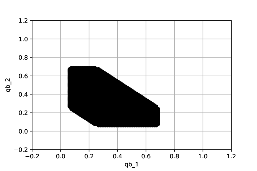
(c). $n=100$

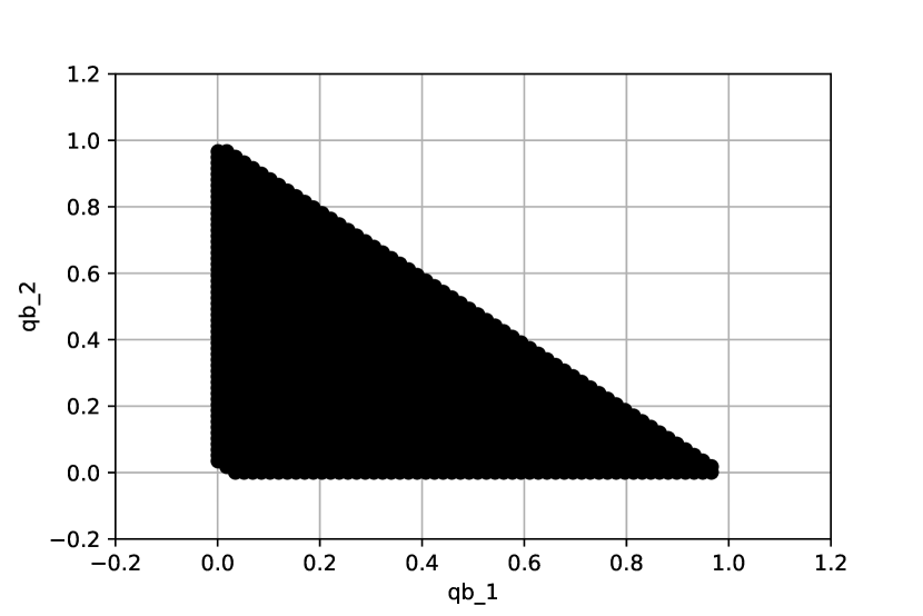
(d). $n=5$

Appendix EC.6 The Optimistic Dual Counterpart

Beck and Ben-Tal, (2009), Gorissen et al., (2014) and Gorissen and den Hertog, (2015) have shown that a robust minimization problem with a compact convex uncertainty set can also be reformulated by maximizing the dual of its uncertain problem over all uncertain variables. In this section, we aim to derive the optimistic dual counterpart of the robust problem

$$\min_{\mathbf{a}\in\mathcal{A},c\in\mathcal{C}}\left\{\mathbf{a}^{T}\mathbf{d}+\zeta\cdot c\leavevmode\nobreak\ \middle|\leavevmode\nobreak\ \sup_{(\mathbf{q},\bar{\mathbf{q}})\in\mathcal{U}_{\phi,h}(\mathbf{p})}-\sum^{m}_{i=1}\bar{q}_{i}u(f(\mathbf{a},\mathbf{x}_{i}))\leq c\right\},$$ (EC.34)

where

$$\mathcal{U}_{\phi,h}(\mathbf{p})=\left\{(\mathbf{q},\bar{\mathbf{q}})\in\mathbb{R}^{2m}\;\begin{tabular}[]{|l}$\sum^{m}_{i=1}q_{i}=\sum^{m}_{i=1}\bar{q}_{i}=1$\\ $\sum^{m}_{i=1}p_{i}\phi\left(\frac{q_{i}}{p_{i}}\right)\leq r$\\ $\sum_{i\in J}\bar{q}_{i}\leq h\left(\sum_{i\in J}q_{i}\right),\leavevmode\nobreak\ \forall J\subset[m]$\\ $q_{i},\bar{q}_{i}\geq 0,\leavevmode\nobreak\ \forall i=1,\ldots,m$\end{tabular}\right\}.$$

Here, we have either $(\mathcal{C}=\mathbb{R},\mathbf{d}=\mathbf{0},\zeta=1)$, or $(\mathcal{C}=\{c_{0}\},\mathbf{d}\neq\mathbf{0},\zeta=0$). Note that $\mathcal{U}_{\phi,h}(\mathbf{p})$ is a compact set since it is bounded and closed due to Assumption 3 that the functions $\phi,-h$ are lower-semicontinuous convex functions.

To derive the optimistic dual counterpart of (EC.34), we first consider its uncertain problem, which for a given $(\mathbf{q},\mathbf{\bar{q}})\in\mathcal{U}_{\phi,h}(\mathbf{p})$ is defined as

$$\begin{split}&\min_{\mathbf{a}\in\mathcal{A},c\in\mathcal{C}}\left\{\mathbf{a}^{T}\mathbf{d}+\zeta\cdot c\leavevmode\nobreak\ \middle|\leavevmode\nobreak\ -\sum^{m}_{i=1}\bar{q}_{i}u(f(\mathbf{a},\mathbf{x}_{i}))\leq c\right\}\\ &=\min_{\mathbf{a}\in\mathbb{R}^{I},c\in\mathcal{C}}\left\{\mathbf{a}^{T}\mathbf{d}+\zeta\cdot c\leavevmode\nobreak\ \middle|\leavevmode\nobreak\ -\sum^{m}_{i=1}\bar{q}_{i}u(f(\mathbf{a},\mathbf{x}_{i}))\leq c,f_{i}(\mathbf{a})\leq 0,i=1,\ldots,L\right\}.\end{split}$$ (EC.35)

Recall that $\mathcal{A}$ is a set represented by convex inequalities, hence we can express it as $\mathcal{A}=\{\mathbf{a}\in\mathbb{R}^{I}|f_{i}(\mathbf{a})\leq 0,i=1,\ldots,L\}$, for some convex functions $f_{i}$’s. Assume that (EC.35) satisfies Slater’s condition and is bounded from below. Then, the dual of (EC.35) is

$$\max_{y_{0},\ldots,y_{L}\geq 0}\inf_{\mathbf{a}\in\mathbb{R}^{I},c\in\mathcal{C}}\left\{\mathbf{a}^{T}\mathbf{d}+\zeta\cdot c-y_{0}\sum^{m}_{i=1}\bar{q}_{i}u(f(\mathbf{a},\mathbf{x}_{i}))-y_{0}c+\sum^{L}_{k=1}y_{k}f_{k}(\mathbf{a})\right\}.$$ (EC.36)

The optimistic dual counterpart is defined by maximizing the dual over all uncertain variables in the uncertainty set, i.e.,

$$\sup_{(\mathbf{q},\mathbf{\bar{q}})\in\mathcal{U}_{\phi,h}(\mathbf{p})}\max_{y_{0},\ldots,y_{L}\geq 0}\inf_{\mathbf{a}\in\mathbb{R}^{I},c\in\mathcal{C}}\left\{\mathbf{a}^{T}\mathbf{d}+\zeta\cdot c-y_{0}\sum^{m}_{i=1}\bar{q}_{i}u(f(\mathbf{a},\mathbf{x}_{i}))-y_{0}c+\sum^{L}_{k=1}y_{k}f_{k}(\mathbf{a})\right\}.$$ (OD)

The following theorem states a reformulation of (OD).

Theorem EC.6.1.

The optimistic dual counterpart (OD) is equivalent to the following concave problem.

$$\begin{split}\hfil\displaystyle\begin{split}\sup_{\begin{subarray}{c}\mathbf{z},\mathbf{\bar{z}}\in\mathbb{R}^{m}_{\geq 0}\\ y_{0},\ldots,y_{L}\geq 0\\ \boldsymbol{\lambda}_{1},\ldots,\boldsymbol{\lambda}_{m},\boldsymbol{\eta}_{1},\ldots,\boldsymbol{\eta}_{L}\in\mathbb{R}^{I}\end{subarray}}&-\sum^{m}_{i=1}\bar{z}_{i}(-u\circ f)^{*}\left(\frac{\mathbf{\boldsymbol{\lambda}}_{i}}{y_{0}\bar{q}_{i}},\mathbf{x}_{i}\right)-\sum^{L}_{k=1}y_{k}(f_{k})^{*}\left(\frac{\boldsymbol{\eta}_{k}}{y_{k}}\right)-y_{0}c_{0}\mathbbm{1}_{\{\zeta=0\}}\\ \mathrm{subject}\leavevmode\nobreak\ \mathrm{to}&\leavevmode\nobreak\ \sum^{m}_{i=1}\boldsymbol{\lambda}_{i}=-\sum^{L}_{k=1}\boldsymbol{\eta}_{k}-\mathbf{d}\\ &\sum^{m}_{i=1}z_{i}=\sum^{m}_{i=1}\bar{z}_{i}=y_{0}\\ &\sum_{i\in I}\bar{z}_{i}-y_{0}h\left(\frac{\sum_{i\in I}z_{i}}{y_{0}}\right)\leq 0,\forall I\in 2^{N}_{-},\\ &\sum^{m}_{i=1}y_{0}p_{i}\phi\left(\frac{z_{i}}{y_{0}p_{i}}\right)-y_{0}r\leq 0,\end{split}\end{split}$$ (EC.37)

where $\mathbf{z}=y_{0}\mathbf{q}$ and $\mathbf{\bar{z}}=y_{0}\mathbf{\bar{q}}$. If the Slater’s condition holds for problem (EC.37), then (EC.34) is equal to (EC.37). Moreover, the KKT-vector of (EC.37) corresponding to the dual equality constraints $\sum^{m}_{i=1}\boldsymbol{\lambda}_{i}=-\sum^{L}_{k=1}\boldsymbol{\eta}_{k}-\mathbf{d}$ gives the optimal solution of (EC.34).

Proof.

By Theorem 1 of Gorissen and den Hertog, (2015), it only remains to reformulate (OD). We have that,

$$\inf_{\mathbf{a}\in\mathbb{R}^{I},c\in\mathcal{C}}\left\{\mathbf{a}^{T}\mathbf{d}+\zeta\cdot c-y_{0}\sum^{m}_{i=1}\bar{q}_{i}u(f(\mathbf{a},\mathbf{x}_{i}))-y_{0}c+\sum^{L}_{k=1}y_{k}f_{k}(\mathbf{a})\right\}$$

$$=\inf_{\mathbf{a}\in\mathbb{R}^{I}}\left\{\mathbf{a}^{T}\mathbf{d}-y_{0}\sum^{m}_{i=1}\bar{q}_{i}u(f(\mathbf{a},\mathbf{x}_{i}))+\sum^{L}_{k=1}y_{k}f_{k}(\mathbf{a})\right\}+\inf_{c\in\mathcal{C}}(\zeta-y_{0})c$$

$$=-\sup_{\mathbf{a}\in\mathbb{R}^{I}}\left\{-\mathbf{a}^{T}\mathbf{d}+y_{0}\sum^{m}_{i=1}\bar{q}_{i}u(f(\mathbf{a},\mathbf{x}_{i}))-\sum^{L}_{k=1}y_{k}f_{k}(\mathbf{a})\right\}+\inf_{c\in\mathcal{C}}(\zeta-y_{0})c.$$

Note that since $\mathcal{C}$ is either $\mathbb{R}$ if $\zeta=1$ or $\{c_{0}\}$ for some $c_{0}\in\mathbb{R}$, if $\zeta=0$. Hence, we have that

$$\inf_{c\in\mathcal{C}}(\zeta-y_{0})c=\begin{cases}-y_{0}c_{0}&\leavevmode\nobreak\ \text{if}\leavevmode\nobreak\ \mathcal{C}=c_{0}\\ 0&\leavevmode\nobreak\ \text{if}\leavevmode\nobreak\ \mathcal{C}=\mathbb{R},\leavevmode\nobreak\ y_{0}=1\\ -\infty&\leavevmode\nobreak\ \text{else}.\end{cases}$$

We examine the left supremum term. We have,

$$\sup_{\mathbf{a}\in\mathbb{R}^{I}}\left\{-\mathbf{a}^{T}\mathbf{d}+y_{0}\sum^{m}_{i=1}\bar{q}_{i}u(f(\mathbf{a},\mathbf{x}_{i}))-\sum^{L}_{k=1}y_{k}f_{k}(\mathbf{a})\right\}$$

$$=\sup_{\begin{subarray}{c}\mathbf{a},\mathbf{w}_{1},\ldots,\mathbf{w}_{m},\\ \mathbf{v}_{1},\ldots,\mathbf{v}_{L}\in\mathbb{R}^{I}\end{subarray}}\left\{-\mathbf{a}^{T}\mathbf{d}+y_{0}\sum^{m}_{i=1}\bar{q}_{i}u(f(\mathbf{w}_{i},\mathbf{x}_{i}))-\sum^{L}_{k=1}y_{k}f_{k}(\mathbf{v}_{k})\leavevmode\nobreak\ \middle|\leavevmode\nobreak\ \mathbf{w}_{i}=\mathbf{a},\leavevmode\nobreak\ \mathbf{v}_{k}=\mathbf{a},i\in[m],k\in[L]\right\}$$

$$=\inf_{\begin{subarray}{c}\boldsymbol{\lambda}_{1},\ldots\boldsymbol{\lambda}_{m},\\ \boldsymbol{\eta}_{1},\ldots,\boldsymbol{\eta}_{L}\in\mathbb{R}^{I}\end{subarray}}\sup_{\begin{subarray}{c}\mathbf{a},\mathbf{w}_{1},\ldots,\mathbf{w}_{m},\\ \mathbf{v}_{1},\ldots,\mathbf{v}_{L}\in\mathbb{R}^{I}\end{subarray}}\left\{-\mathbf{a}^{T}\mathbf{d}+\sum^{m}_{i=1}\mathbf{\boldsymbol{\lambda}}_{i}^{T}(\mathbf{w}_{i}-\mathbf{a})+\sum^{L}_{k=1}\mathbf{\boldsymbol{\eta}}_{k}^{T}(\mathbf{v}_{k}-\mathbf{a})+y_{0}\sum^{m}_{i=1}\bar{q}_{i}u(f(\mathbf{w}_{i},\mathbf{x}_{i}))-\sum^{L}_{k=1}y_{k}f_{k}(\mathbf{v}_{k})\right\}$$

$$=\inf_{\begin{subarray}{c}\boldsymbol{\lambda}_{1},\ldots\boldsymbol{\lambda}_{m},\\ \boldsymbol{\eta}_{1},\ldots,\boldsymbol{\eta}_{L}\in\mathbb{R}^{I}\end{subarray}}\sup_{\begin{subarray}{c}\mathbf{a},\mathbf{w}_{1},\ldots,\mathbf{w}_{m},\\ \mathbf{v}_{1},\ldots,\mathbf{v}_{L}\in\mathbb{R}^{I}\end{subarray}}\left\{-\left(\sum^{m}_{i=1}\boldsymbol{\lambda}_{i}+\sum^{L}_{k=1}\boldsymbol{\eta}_{k}+\mathbf{d}\right)^{T}\mathbf{a}+\sum^{m}_{i=1}\boldsymbol{\lambda}_{i}^{T}\mathbf{w}_{i}-y_{0}\bar{q}_{i}(-u)(f(\mathbf{w}_{i},\mathbf{x}_{i}))\right.$$

$$\qquad\qquad\qquad\qquad\left.+\sum^{L}_{k=1}\boldsymbol{\eta}_{k}^{T}\mathbf{v}_{k}-y_{k}f_{k}(\mathbf{v}_{k})\right\}$$

$$=\inf_{\begin{subarray}{c}\boldsymbol{\lambda}_{1},\ldots\boldsymbol{\lambda}_{m},\\ \boldsymbol{\eta}_{1},\ldots,\boldsymbol{\eta}_{L}\in\mathbb{R}^{I}\end{subarray}}\left\{\sum^{m}_{i=1}y_{0}\bar{q}_{i}(-u\circ f)^{*}\left(\frac{\mathbf{\boldsymbol{\lambda}}_{i}}{y_{0}\bar{q}_{i}},\mathbf{x}_{i}\right)+\sum^{L}_{k=1}y_{k}(f_{k})^{*}\left(\frac{\boldsymbol{\eta}_{k}}{y_{k}}\right)\leavevmode\nobreak\ \middle|\leavevmode\nobreak\ \sum^{m}_{i=1}\boldsymbol{\lambda}_{i}=-\sum^{L}_{k=1}\boldsymbol{\eta}_{k}-\mathbf{d}\right\},$$

where $(-u\circ f)$ denotes the composition function of the two. Similar to Gorissen and den Hertog, (2015), a change of variables $\mathbf{z}=y_{0}\mathbf{q}$ and $\mathbf{\bar{z}}=y_{0}\mathbf{\bar{q}}$ and multiplying the constraints in $\mathcal{U}_{\phi,h}(\mathbf{p})$ by $y_{0}$ yields the desired statement. ∎

Appendix EC.7 The Hit-and-Run Algorithm

In this section, we explain how the Hit-and-Run algorithm is applied to generate a uniform sample on the $\phi$-divergence set. Let $S$ be an open subset in $\mathbb{R}^{d}$. The general procedure of the Hit-and-Run algorithm is fairly simple. Start with an interior point $x_{0}\in S$. Choose uniformly a random direction $u\in\partial\mathcal{D}$ where $\partial\mathcal{D}=\{x\in\mathbb{R}^{d}:\|x\|_{2}=1\}$. Draw uniformly a scalar $\lambda\in\{\lambda\in\mathbb{R}:x_{0}+\lambda u\in S\}$ and then update $x_{0}$ with $x_{0}+\lambda u$. It is shown by Bélisle et al., (1993) that for a convex set $S$, this sampling process will converge to a uniform sampling on $S$.
To apply the Hit-and-Run algorithm to the $\phi$-divergence uncertainty set, we first re-parametrize the set. Recall the definition of the $\phi$-divergence set

$$\mathcal{D}_{\phi}(\mathbf{p},r)\triangleq\{\mathbf{q}\in\mathbb{R}^{m}\leavevmode\nobreak\ |\leavevmode\nobreak\ \mathbf{q}\geq\mathbf{0},\mathbf{q}^{T}\mathbf{1}=1,\sum^{m}_{i=1}p_{i}\phi\left(\frac{q_{i}}{p_{i}}\right)\leq r\}.$$

Using the equality $\mathbf{q}^{T}\mathbf{1}=1$, it is clear that we can parametrize the $\phi$-divergence set with the following set

$$\tilde{\mathcal{D}}_{\phi}(\mathbf{q}|\mathbf{p},r)\triangleq\{\mathbf{q}\in\mathbb{R}^{m-1}|\mathbf{q}\geq\mathbf{0},1-\sum^{m-1}_{i=1}q_{i}\geq 0,\sum^{m-1}_{i=1}p_{i}\phi\left(\frac{q_{i}}{p_{i}}\right)+p_{m}\phi\left(\frac{1-\sum^{m-1}_{i=1}q_{i}}{p_{m}}\right)\leq r\}.$$ (EC.38)

Since this is a set with convex inequalities, and often we assume Slater’s condition, its interior is an open convex set. Hence, we can apply the Hit-and-Run algorithm to obtain a uniform sample of the interior of $\tilde{\mathcal{D}}_{\phi}(\mathbf{q}|\mathbf{p},r)$ and thus also the interior of $\mathcal{D}_{\phi}(\mathbf{p},r)$ due to the one-to-one correspondence. The precise procedure will be the following.

• We start with the nominal vector $\mathbf{q}_{k}=(p_{1},\ldots,p_{m-1})$. We draw a uniform element $\mathbf{u}\in\partial\mathcal{D}$ for dimension $d=m-1$. This is done by drawing $m-1$ a standard normal i.i.d. sample $X_{1},\ldots X_{m-1}$ and then renormalize it. This method is proposed by Muller, (1959). It follows from the property that the joint density $f((x_{1},\ldots,x_{d}))=\frac{1}{(\sqrt{2\pi})^{d}}e^{-\frac{1}{2}\|(x_{1},\ldots,x_{d})\|_{2}}$ is only norm-dependent.

• Given $\mathbf{u}$ and $\mathbf{q}_{k}$. We will then determine the set $\Lambda\triangleq\{\lambda\in\mathbb{R}:\mathbf{q}_{k}+\lambda\mathbf{u}\in\tilde{\mathcal{D}}_{\phi}(\mathbf{q}|\mathbf{p},r)\}$. By convexity, we have if $\lambda\in\Lambda$ and $\lambda>0$, then all scalars in $[0,\lambda]$ also lies in $\Lambda$. Similarly, it holds for $\lambda<0$. Since $\tilde{\mathcal{D}}_{\phi}(\mathbf{q}|\mathbf{p},r)$ is also bounded, there exists $\lambda_{\min},\lambda_{\max}$ such that $[\lambda_{\min},\lambda_{\max}]=\Lambda$. Both values can be found using a bisection search.

• We draw a random $\lambda\in[\lambda_{\min},\lambda_{\max}]$ update $\mathbf{q}_{k+1}=\mathbf{q}_{k}+\lambda\mathbf{u}$. We then repeat the process.

Appendix EC.8 SOS2-Constraints Formulation

Let $u:[l_{0},u_{0}]\to\mathbb{R}$ be a non-decreasing, piecewise-linear utility function defined on some interval $[l_{0},u_{0}]$ that contains the image set $\{\mathbf{a}^{T}\mathbf{x}_{i}\leavevmode\nobreak\ |\leavevmode\nobreak\ \mathbf{a}\in\mathcal{A},i\in[m]\}$. Let $\{t_{j},u(t_{j})\}^{K}_{j=1}$ be the support points of $u$, where $l_{0}=t_{1}<\cdots<t_{K}=u_{0}$. Then, the constraints in (53) can be formulated using the following bilinear and SOS2 constraints:

$$\begin{cases}\beta\cdot h(p^{0})+\sum^{K_{1}}_{k=1}\nu_{k}b^{(1)}_{k}+\sum^{m}_{i=1}\sum^{K_{1}}_{k=1}\lambda_{ik}l^{(1)}_{k}p_{i}-\sum^{m}_{i=1}\bar{q}_{i}z_{i}\leq c\\ -z_{i}-\beta-\sum^{K_{1}}_{k=1}\lambda_{ik}\leq 0,\quad\forall i\in[m]\\ \lambda_{ik}\leq\nu_{k},\quad\forall i\in[m],\leavevmode\nobreak\ \forall k\in[K_{1}]\\ \bar{q}_{i}\leq l^{(2)}_{k}p_{i}+t_{ik},\quad\forall i\in[m],\leavevmode\nobreak\ \forall k\in[K_{2}]\\ \sum^{m}_{i=1}t_{ik}\leq b^{(2)}_{k},\quad\forall k\in[K_{2}]\\ \sum^{m}_{i=1}\bar{q}_{i}=\bar{h}(1-p^{0})\\ \mathbf{a}^{T}\mathbf{x}_{i}=\sum^{K}_{j=1}\tilde{\lambda}_{ij}t_{j},\leavevmode\nobreak\ \forall i\in[m]\\ z_{i}=\sum^{K}_{j=1}\tilde{\lambda}_{ij}u(t_{j})\leavevmode\nobreak\ \forall i\in[m]\\ \sum^{K}_{j=1}\tilde{\lambda}_{ij}=1,\leavevmode\nobreak\ \forall i\in[m]\\ \tilde{\lambda}_{ij}\geq 0,\leavevmode\nobreak\ \mathrm{SOS}2,\leavevmode\nobreak\ \forall j\in[K],\leavevmode\nobreak\ i\in[m].\end{cases}$$ (EC.39)

References

- Allais, (1953) Allais, M. (1953). Le comportement de l’homme rationnel devant le risque: Critique des postulats et axiomes de l’école américaine. Econometrica, 21:503–546.
- Beck and Ben-Tal, (2009) Beck, A. and Ben-Tal, A. (2009). Duality in robust optimization: Primal worst equals dual best. Operations Research Letters, 37:1–6.
- Ben-Tal et al., (1991) Ben-Tal, A., Ben-Israel, A., and Teboulle, M. (1991). Certainty equivalents and information measures: Duality and extremal Principles. Journal of Mathematical Analysis And Applications, 157(1):211–236.
- Ben-Tal et al., (2013) Ben-Tal, A., den Hertog, D., de Waegenaere, A., Melenberg, B., and Rennen, G. (2013). Robust solutions of optimization problems affected by uncertain probabilities. Management Science, 59(2):341–357.
- Ben-Tal and Nemirovski, (2019) Ben-Tal, A. and Nemirovski, A. (2019). Lectures on Modern Convex Optimization. SIAM.
- Ben-Tal and Teboulle, (1986) Ben-Tal, A. and Teboulle, M. (1986). Expected utility, penalty functions, and duality in stochastic nonlinear programming. Management Science, 32(11):1445–1466.
- Ben-Tal and Teboulle, (1987) Ben-Tal, A. and Teboulle, M. (1987). Penalty functions and duality in stochastic programming via -divergence functionals. Mathematics of Operations Research, 12(2):224–240.
- Ben-Tal and Teboulle, (2007) Ben-Tal, A. and Teboulle, M. (2007). An old-new concept of convex risk measures: The optimized certainty equivalent. Mathematical Finance, 17(3):449–476.
- Berge, (1963) Berge, C. (1963). Topological Spaces: Including a Treatment of Multi-Valued Functions, Vector Spaces, and Convexity. Courier Corporation.
- Bertsimas and Brown, (2009) Bertsimas, D. and Brown, D. B. (2009). Constructing uncertainty sets for robust linear optimization. Operations Research, 57(6):1483–1495.
- Bertsimas and den Hertog, (2022) Bertsimas, D. and den Hertog, D. (2022). Robust and Adaptive Optimization. Dynamic Ideas LLC Belmont, Massachusetts.
- Bertsimas et al., (2016) Bertsimas, D., Dunning, I., and Lubin, M. (2016). Reformulation versus cutting-planes for robust optimization. Computational Management Science, 13(2):195–217.
- Bélisle et al., (1993) Bélisle, C. J., Romeijn, H. E., and Smith, R. L. (1993). Hit-and-Run algorithms for generating multivariate distributions. Mathematics of Operations Research, 18(2):255–266.
- Cai et al., (2023) Cai, J., Li, J. Y.-M., and Mao, T. (2023). Distributionally robust optimization under distorted expectations. Operations Research, 0(0).
- Carlier and Dana, (2006) Carlier, G. and Dana, R.-A. (2006). Law invariant concave utility functions and optimization problems with monotonicity and comonotonicity constraints. Statistics & Risk Modeling, 24(1):127–152.
- Chares, (2009) Chares, P. R. (2009). Cones and Interior-Point Algorithms for Structured Convex Optimization Involving Powers and Exponentials. Ecole polytechnique de Louvain, Université catholique de Louvain.
- Chew et al., (1987) Chew, S., Karni, E., and Safra, Z. (1987). Risk aversion in the theory of expected utility with rank dependent probabilities. Journal of Economic Theory, 42:370–381.
- Choquet, (1954) Choquet, G. (1954). Theory of capacities. Annales de l’Institut Fourier, 5:131–295.
- Cox, (1971) Cox, M. (1971). An algorithm for approximating convex functions by means by first degree splines. The Computer Journal, 14(3):272–275.
- Csiszár, (1975) Csiszár, I. (1975). -divergence geometry of probability distributions and minimization problems. Annals of Probability, 3:146–158.
- Delage et al., (2022) Delage, E., Guo, S., and Xu, H. (2022). Shortfall risk models when information of loss function is incomplete. Operations Research, 70(6):3511–3518.
- Denneberg, (1994) Denneberg, D. (1994). Non-Additive Measure and Integral. Springer.
- Eeckhoudt and Laeven, (2021) Eeckhoudt, L. R. and Laeven, R. J. (2021). Dual moments and risk attitudes. Operations Research, 70(3):1330–1341.
- Eeckhoudt et al., (2020) Eeckhoudt, L. R., Laeven, R. J., and Schlesinger, H. (2020). Risk apportionment: The dual story. Journal of Economic Theory, 185:104971.
- Esfahani and Kuhn, (2018) Esfahani, P. M. and Kuhn, D. (2018). Data-driven distributionally robust optimization using the Wasserstein metric: Performance guarantees and tractable reformulations. Mathematical Programming, 171:115–166.
- Föllmer and Schied, (2016) Föllmer, H. and Schied, A. (2016). Stochastic Finance, 4th ed. Berlin: De Gruyter.
- Gilboa and Schmeidler, (1989) Gilboa, I. and Schmeidler, D. (1989). Maxmin expected utility with non-unique prior. Journal of Mathematical Economics, 18(2):141–153.
- Goovaerts and Laeven, (2008) Goovaerts, M. J. and Laeven, R. J. A. (2008). Actuarial risk measures for financial derivative pricing. Insurance: Mathematics and Economics, 42(2):540–547.
- Gorissen et al., (2014) Gorissen, B. L., Blanc, H., Ben-Tal, A., and den Hertog, D. (2014). Technical Note- Deriving robust and globalized robust solutions of uncertain linear programs with general convex uncertainty sets. Operations Research, 62(3):672–679.
- Gorissen and den Hertog, (2015) Gorissen, B. L. and den Hertog, D. (2015). Robust nonlinear optimization via the dual. Optimizations Online.
- Gurobi Optimization, LLC, (2023) Gurobi Optimization, LLC (2023). Gurobi Optimizer Reference Manual.
- Hansen and Sargent, (2001) Hansen, L. P. and Sargent, T. J. (2001). Robust control and model uncertainty. American Economic Review, 91:60–66.
- Hansen and Sargent, (2007) Hansen, L. P. and Sargent, T. J. (2007). Robustness. Princeton University Press, stu-student edition.
- He and Zhou, (2011) He, X. D. and Zhou, X. Y. (2011). Portfolio choice via quantiles. Mathematical Finance, 21(2):203–231.
- Huber, (1981) Huber, P. J. (1981). Robust Statistics. Wiley, New York.
- Imamoto and Tang, (2008) Imamoto, A. and Tang, B. (2008). Optimal piecewise linear approximation of convex functions . Proceedings of the World Congress on Engineering and Computer Science.
- Laeven and Stadje, (2023) Laeven, R. J. and Stadje, M. (2023). A rank-dependent theory for decision under risk and ambiguity. Technical Report.
- Maccheroni et al., (2006) Maccheroni, F., Marinacci, M., and Rustichini, A. (2006). Ambiguity aversion, robustness, and the variational representation of preferences. Econometrica, 74(6):1447–1498.
- Muller, (1959) Muller, M. E. (1959). A note on a uniformly method for generating points on -dimensional spheres. Commun. Ass. Comput. Math., 2(4):19–20.
- Mutapcic and Boyd, (2009) Mutapcic, A. and Boyd, S. (2009). Cutting-set methods for robust convex optimization with pessimizing oracles. Optimization Methods & Software, 24(3):381–406.
- Pardo, (2006) Pardo, L. (2006). Statistical Inference Based on Divergence Measures. Chapman & Hall/ CRC Boca Raton.
- Pesenti et al., (2020) Pesenti, S., Wang, Q., and Wang, R. (2020). Optimizing distortion riskmetrics with distributional uncertainty. Paper. Available on ArXiv.
- Postek et al., (2016) Postek, K., den Hertog, D., and Melenberg, B. (2016). Computationally tractable counterparts of distributionally robust constraints on risk measures. SIAM Review, 58(4):603–650.
- Prelec, (1998) Prelec, D. (1998). The probability weighting function. Econometrica, 66(3):497–527.
- Quiggin, (1982) Quiggin, J. (1982). A theory of anticipated utility. Journal of Economic Behavior and Organization, 3(4):323–343.
- Rockafellar, (1970) Rockafellar, R. T. (1970). Convex Analysis. Princeton University Press, Princeton, NJ.
- Ryoo and Sahinidis, (1996) Ryoo, H. S. and Sahinidis, N. V. (1996). A branch-and-reduce approach to global optimization. Journal of Global Optimization, 8(2):107–138.
- Schmeidler, (1986) Schmeidler, D. (1986). Integral representation without additivity. Proceedings of the American Mathematical Society, 97:255–261.
- Schmeidler, (1989) Schmeidler, D. (1989). Subjective probability and expected utility without additivity. Econometrica, 57(3):571–587.
- Tversky and Kahneman, (1992) Tversky, A. and Kahneman, D. (1992). Advances in prospect theory: Cumulative representation of uncertainty. Journal of Risk and Uncertainty, 5:297–323.
- von Neumann and Morgenstern, (1944) von Neumann, J. and Morgenstern, O. (1944). Theory of Games and Economic Behavior. Princeton University Press, Princeton, 3 edition.
- Wakker, (2010) Wakker, P. P. (2010). Prospect Theory for Risk and Rationality. Cambridge University Press.
- Wald, (1950) Wald, A. (1950). Statistical Decision Functions. Wiley, New York.
- Wang, (2000) Wang, S. S. (2000). A class of distortion operators for pricing financial and insurance risks. The Journal of Risk and Insurance, 67(1):15–36.
- Wang and Xu, (2023) Wang, W. and Xu, H. (2023). Preference robust distortion risk measure and its application. Mathematical Finance, 33(2).
- Wiesemann et al., (2014) Wiesemann, W., Kuhn, D., and Sim, M. (2014). Distributionally robust convex optimization. Operations Research, 62(6):1358–1376.
- Yaari, (1987) Yaari, M. E. (1987). The dual theory of choice under risk. Econometrica, 55(1):95–115.