Parallel-in-Time Kalman Smoothing Using Orthogonal Transformations

Abstract

We present a numerically-stable parallel-in-time linear Kalman smoother. The smoother uses a novel highly-parallel QR factorization for a class of structured sparse matrices for state estimation, and an adaptation of the SelInv selective-inversion algorithm to evaluate the covariance matrices of estimated states. Our implementation of the new algorithm, using the Threading Building Blocks (TBB) library, scales well on both Intel and ARM multi-core servers, achieving speedups of up to 47x on 64 cores. The algorithm performs more arithmetic than sequential smoothers; consequently it is 1.8x to 2.5x slower on a single core. The new algorithm is faster and scales better than the parallel Kalman smoother proposed by Särkkä and García-Fernández in 2021.

1 Introduction

(0cm, -12.5cm) © 2025 IEEE. Personal use of this material is permitted. Permission from IEEE must be obtained for all other uses, in any current or future media, including reprinting/republishing this material for advertising or promotional purposes, creating new collective works, for resale or redistribution to servers or lists, or reuse of any copyrighted component of this work in other works.
Accepted to the IEEE International Parallel & Distributed Processing Symposium (IPDPS), 2025. Kalman smoothing and filtering aim to estimate a sequence of (usually hidden) states of a dynamic system from noisy and often indirect observations of the different states. The dynamic system is defined by inexact evolution or state equations that relate each state to its immediate predecessor. Noisy (inexact) observation equations relate each vector of simultaneous observations to the state at that time. Both the evolution/state equations and the observation equations can be linear or nonlinear. Kalman filters and smoothers estimate the states using generalized least-squares minimization of the noise (error) terms in the equations. The weighting of the noise terms is determined by their assumed variance/covariance. The minimization is exact when the equations are linear; it is often inexact when some of the equations are nonlinear.

In Kalman smoothing, we process an entire batch of observations that has been collected. Thus, the estimation of each particular state depends on observations of that state and all its predecessors in the batch, as well as on observations of all successor states. Kalman filtering is a simpler variant in which each state is estimated by observations of itself and of predecessors. Kalman filtering has numerous applications in which real-time state estimates are required. Kalman smoothing is used to post process data to obtain the best possible estimates of whole trajectories.

The first efficient linear Kalman filtering algorithm was invented in 1960 [1]. It was extended to smoothing a few years later [2]. Until recently, all Kalman filtering and smoothing algorithms have been highly sequential, processing one state at a time. Filtering algorithms use a single forward-in-time pass over the data (the observations). Sequential linear smoothing algorithms consist of one forward pass and one backward pass. In 2021, Särkkä and García-Fernández introduced the first parallel-in-time linear Kalman smoother [3]. It is based on a clever restructuring of both the forward and backward passes in a conventional Kalman smoother as generalized prefix sums with appropriately-defined associative operations, enabling the use of a parallel-prefix algorithm to estimate the states and their covariance matrices.

In this paper we introduce a novel and completely different parallel linear Kalman smoother with key advantages over the Särkkä and García-Fernández smoother, including higher performance in all cases. Our algorithm, which we refer to as Odd-Even Kalman smoothing, is based on a specialized sparse QR factorization of the coefficient matrix of the linear least-squares problem that underlies Kalman smoothing. The factorization is highly parallel thanks to a recursive odd-even permutation of block columns of the matrix. This idea is inspired by odd-even reduction (also called cyclic reduction), a family of algorithms for solving block tridiagonal systems of linear equations [4, 5]. While this QR factorization allows us to estimate the smoothed states efficiently in parallel, it does not provide a way to compute the covariance matrices of these estimates.

To compute the covariance matrices of the estimates, we adapt an algorithm called SelInv [6]. This algorithm uses the sparse triangular factor of a symmetric matrix to computes certain blocks of the inverse of the matrix. We show how to adapt this algorithm to the Kalman smoothing case, that it computes the necessary covariance matrices, and that in our case it is both efficient and highly parallel.

We implemented two variants of this algorithm, as well as the Särkkä and García-Fernández algorithm, in a state-of-the-art parallel-programming environment. We tested them on multi-core servers with 36, 56, and 64 cores. (To the best of our knowledge, parallelism in the Särkkä and García-Fernández algorithm was never evaluated experimentally.) We also implemented the best sequential variants of the algorithms. We show that the parallel algorithms outperform the sequential ones and that our new algorithm is almost always faster than the Särkkä and García-Fernández algorithm. On the other hand, the experiments show that the parallel algorithms do have a constant work overhead, in the sense that they perform more arithmetic than the sequential ones, between 1.8x and 2.5x for the two variants of our algorithm and 1.8–2.6x for the algorithm of Särkkä and García-Fernández.

The rest of this article is structured as follows. Section 2 describes background and related work. Section 3 describes our new parallel QR factorization. Section 4 explains how we compute the covariance matrices of the estimated states. We describe our implementation and experimental results in Section 5, and we present our conclusions in Section 6.

2 Background and Related Work

2.1 Kalman Filtering and Smoothing Problems

Kalman smoothing estimates all the states of a discrete-in-time dynamic system that has been observed for some time [7]. We denote the instantaneous state of the system at time $t_{i}$ by $u_{i}\in\mathbb{R}^{n_{i}}$. We refer to $u_{i}$ as the state of state $i$. The state $u_{i}$ satisfies a recurrence called the evolution equation or state equation and possibly a constraint called the observation equation. We do not require all the states to have the same dimension, although the uniform-dimension case is very common. The evolution equation has the form

$$H_{i}u_{i}=\mathcal{F}_{i}\left(u_{i-1}\right)+c_{i}+\epsilon_{i}\;,$$ (1)

where $H_{i}\in\mathbb{R}^{\ell_{i}\times n_{i}}$ is a known full-rank matrix, $\mathcal{F}_{i}:\mathbb{R}^{n_{i-1}}\rightarrow\mathbb{R}^{\ell_{i}}$ is a known function (often assumed to be continuously differentiable), $c_{i}\in\mathbb{R}^{\ell_{i}}$ is a known vector that represents external forces, and $\epsilon_{i}$ is an unknown noise or error vector. The matrix $H_{i}$ is often assumed to be the identity matrix, but we do not require this (and do not require it to be square). A rectangular $H_{i}$ allow modeling systems in which the dimension of the state vector increases or decreases [8]. Obviously, the first state $u_{0}$ that we model is not defined by an evolution recurrence.

Some of the state vectors $u_{i}$ (but perhaps not all) also satisfy an observation equation of the form

$$o_{i}=\mathcal{G}_{i}\left(u_{i}\right)+\delta_{i}\;,$$ (2)

where $\mathcal{G}_{i}:\mathbb{R}^{n_{i}}\rightarrow\mathbb{R}^{m_{i}}$ is a known function (again usually assumed to be continuously differentiable), $o_{i}\in\mathbb{R}^{m_{i}}$ is a known vector of observations (measurements), and $\delta_{i}$ represents unknown measurement errors or noise. The dimension $m_{i}$ of the observation of $u_{i}$ can vary; it can be smaller than $n_{i}$ (including zero), equal to $n_{i}$, or greater than $n_{i}$.

We use $u$, $b$, and $e$ to denote the concatenations

$$u=\left[\begin{array}[]{c}u_{0}\\ u_{1}\\ u_{2}\\ \vdots\\ u_{k-1}\\ u_{k}\end{array}\right]\;,\quad b=\left[\begin{array}[]{c}o_{0}\\ c_{1}\\ o_{1}\\ \vdots\\ \vdots\\ c_{k}\\ o_{k}\end{array}\right]\;,\quad e=\left[\begin{array}[]{c}\delta_{0}\\ \epsilon_{1}\\ \delta_{1}\\ \vdots\\ \vdots\\ \epsilon_{k}\\ \delta_{k}\end{array}\right]\;.$$

We assume that the $\epsilon_{i}$ terms and the $\delta_{i}$ terms are zero-mean random vectors with known covariance matrices

$$K_{i}=\operatorname{cov}\left(\epsilon_{i}\right)=\operatorname{E}\left(\epsilon_{i}\epsilon_{i}^{T}\right)\;,\quad L_{i}=\operatorname{cov}\left(\delta_{i}\right)=\operatorname{E}\left(\delta_{i}\delta_{i}^{T}\right)$$

that are otherwise uncorrelated,

$$\operatorname{E}\left(\epsilon_{i}\delta_{j}^{T}\right) = 0\;\text{for all}\;i\;\text{and}\;j$$

$$\operatorname{E}\left(\epsilon_{i}\epsilon_{j}^{T}\right) = 0\;\text{for}\;i\neq j$$

$$\operatorname{E}\left(\delta_{i}\delta_{j}^{T}\right) = 0\;\text{for}\;i\neq j\;.$$

That is, we assume that the covariance matrix of $e$ is block diagonal,

$$\operatorname{cov}(e)=\left[\begin{array}[]{cccccc}L_{0}\\ &K_{1}\\ &&L_{1}\\ &&&\ddots\\ &&&&K_{k}\\ &&&&&L_{k}\end{array}\right]\;.$$ (3)

We denote the inverse factors of $L_{i}$ and $K_{i}$ by $V_{i}^{T}V_{i}=K_{i}^{-1}$ and $W_{i}^{T}W_{i}=L_{i}^{-1}$. If we also assume that $e$ is Gaussian, then

$$\begin{bmatrix}\hat{u}_{0}\\ \vdots\\ \hat{u}_{k}\end{bmatrix}=\arg\min\left(\sum_{i=1}^{k}\left(V_{i}\left(H_{i}u_{i}-\mathcal{F}_{i}\left(u_{i-1}\right)-c_{i}\right)\right)^{2}\right.\\ \left.+\sum_{i=0}^{k}\left(W_{i}\left(o_{i}-\mathcal{G}_{i}\left(u_{i}\right)\right)\right)^{2}\right)$$ (4)

is the maximum-likelihood estimator of $u$. If $e$ is not necessarily Gaussian but all $\mathcal{F}_{i}$ and $\mathcal{G}_{i}$ are linear (matrices), the estimator (4) is the minimum-variance unbiased estimator [9]. We normally need not only the $\hat{u}_{i}$s, but also their covariance matrices $\operatorname{cov}(\hat{u}_{i})$. We denote by ${\cal A}(u)$ the nonlinear function that returns the vector

$${\cal A}(u)=\left[\begin{array}[]{c}\mathcal{G}_{0}(u_{0})\\ H_{1}u_{1}-\mathcal{F}_{1}(u_{0})\\ \mathcal{G}_{1}(u_{1})\\ H_{2}u_{2}-\mathcal{F}_{2}(u_{1})\\ \vdots\\ \vdots\\ H_{k}u_{k}-\mathcal{F}_{k}(u_{k-1})\\ \mathcal{G}_{k}(u_{k})\end{array}\right]\;.$$ (5)

With this notation, the least-squares estimator is

$$\hat{u}=\arg\min_{u}\left\|U\left({\cal A}(u)-b\right)\right\|_{2}^{2}$$ (6)

where $U^{T}U=\operatorname{cov}(e)^{-1}$.

In linear Kalman filtering and smoothing, the functions $\mathcal{F}_{i}$ and $\mathcal{G}_{i}$ are real matrices.

2.2 Kalman Filtering/Smoothing Paradigms

The original Kalman filter [1] from 1960 for linear dynamic systems and many of its variants can be derived as formulas that track the expectation and covariance of the state. These algorithms can be extended to smoothers, sometimes called RTS smoothers, using a backward (in time) sweep, to propagate future information back [2]. Good modern references for these algorithms include [10, 7, 9]. Another family of Kalman filter algorithms, sometimes called information filters, track the expectation and the inverse of the covariance matrices of the states. Some variants of these algorithms track a Cholesky factor of the covariance matrix or its inverse. In general, all of these algorithms require the expectation and covariance of the initial state to be known, and some of them can easily handle singular $K_{i}$s and/or singular $L_{i}$s. Most cannot handle rectangular $H_{i}$s.

In 1972 Duncan and Horn realized that when $\operatorname{cov}(e)$ is nonsingular, the Kalman-smoothed trajectory of a linear dynamic system can be expressed as a generalized linear least-squares problem (6) with ${\cal A}$ replaced by a matrix $A$ [11]. In 1977 Paige and Saunders developed a Kalman filter and smoother based on a specialized $UA=QR$ factorization for the special sparsity structure of $UA$ [12]. They also introduced an algorithm to compute $\operatorname{cov}(\hat{u}_{i})$ using a sequence of orthogonal transformations of the $R$ factor. Their algorithm requires $\operatorname{cov}(e)$ to be nonsingular, but it does not require that the expectation of the initial state be known. (Their algorithm also assumes that $H_{i}=I$, but can be easily extended to arbitrary full-rank $H_{i}$s [8].) Due to the use of orthogonal transformation, this algorithm is likely to be more numerically stable than other Kalman filters and smoothers.

All of these algorithms have the same asymptotic efficiency. Assuming that $n_{i}=\Theta(n)$, $\ell_{i}=\Theta(n)$, and $m_{i}=O(n)$ for some state-dimension $n$, Kalman filtering requires $\Theta(n^{3})$ operations per step for a total of $\Theta(kn^{3})$ operations and $\Theta(n^{2})$ storage, and Kalman smoothing requires $\Theta(kn^{3})$ operations and $\Theta(kn^{2})$ storage.

When the $\mathcal{F}_{i}$s and/or $\mathcal{G}_{i}$s are nonlinear, the minimum $\hat{u}$ can be determined using an iterative Gauss-Newton-type algorithm [13]. Each step of the algorithm solves a linear generalized least squares problems of the form (5) but with the $\mathcal{F}_{i}$s and $\mathcal{G}_{i}$s replaced by matrices. These matrices are the Jacobians $F_{i}=\partial\mathcal{F}_{i}/\partial u_{i}$ and $G_{i}=\partial\mathcal{G}_{i}/\partial u_{i}$ evaluated at the estimate of $u$ produced by the previous iteration (or Jacobians concatenated with a diagonal matrix) [14, 15]. That is, Kalman smoothing of a nonlinear dynamic system can be algorithmically reduced to Kalman smoothing of a sequence of linear dynamic systems. The covariance of the states of these linear problems is not needed. (Gauss-Newton algorithms also require an initial guess for $u$, which in the case of dynamic systems can be obtained using an extended or unscented Kalman filter [7] or one of their variants; this step is beyond the scope of this paper.)

2.3 Parallel-in-Time Kalman Smoothing

Kalman filters are incremental (streaming) and therefore inherently sequential, in the sense that they handle step after step. Until recently, all Kalman smoothing algorithms were also sequential, handling step after step with at least one forward sweep in time and one backward sweep in time.

In both filtering and smoothing, the $\Theta(n^{3})$ operations in each step can be parallelized [16], although typical values of $n$ are not large enough to merit that. Generally speaking, these $\Theta(n^{3})$ operations consist of matrix multiplications, matrix factorizations, and solutions of triangular linear systems of equations with multiple right-hand sides. The length of the critical path in practical parallel factorization algorithms and triangular solvers is $\Theta(n)$ (the term critical path refers to the longest chain of dependences; it is also known as span or depth of the computation).

In 2021, Särkkä and García-Fernández introduced the first parallel-in-time linear Kalman smoother [3]. Their algorithm is based on a restructuring of the forward and backward sweeps of the conventional Kalman (RTS) smoother [2] as prefix sums of associative operations operating on the state. Expressing the smoothed trajectory and the covariance matrices $\operatorname{cov}(\hat{u}_{i})$ as quantities computed by two prefix sum operations allows them to be computed using a parallel prefix-sum (parallel scan) algorithm. Särkkä and García-Fernández did not implement the algorithm in a parallel programming environment and did not assess its performance on parallel hardware.

3 A Parallel QR Factorization for Kalman Matrices

We now describe our new parallel QR factorization, which forms the basis for our new smoother. The algorithm is closely related to the Paige-Saunders factorization, but it reorders block columns in order to introduce parallelism.

To efficiently find the minimizer (4), we need to compute, in parallel, a $QR=UAP$ factorization of a column permutation $P$ of a block matrix $UA$ of the form

$$UA=\small\left[\begin{array}[]{cccccc}C_{0}\\ -B_{1}&D_{1}\\ &C_{1}\\ &-B_{2}&D_{2}\\ &&\ddots&\ddots\\ &&&\ddots&\ddots\\ &&&&-B_{k}&D_{k}\\ &&&&&C_{k}\end{array}\right]$$

where $C_{i}=W_{i}G_{i}$, $B_{i}=V_{i}F_{i}$, and $D_{i}=V_{i}H_{i}$. The dimensions of block rows and block columns can vary. To simplify complexity analyses, we assume that the dimensions of all the blocks are $O(n)$ for some $n$. We allow $Q$ to be represented as a product of orthonormal matrices.

We number block columns from $0$ to $k$.

We base the algorithm on the block odd-even reduction (or cyclic reduction) algorithm for block tridiagonal matrices [4, 5]. The algorithm is recursive and it is based on a recursive reordering of the block columns. At the top level, we order the even block columns first,

$$\small\left[\begin{array}[]{ccccc|cccc}C_{0}&&&&\\ -B_{1}&&&&&D_{1}\\ &&&&&C_{1}\\ &D_{2}&&&&-B_{2}\\ &C_{2}&&&\\ &-B_{3}&&&&&D_{3}\\ &&&&&&C_{3}\\ &&D_{4}&&&&-B_{4}\\ &&\vdots&&&&&\ddots\\ &&&&&&&&D_{k-1}\\ &&&\ddots&&&&&C_{k-1}\\ &&&&D_{k}&&&&-B_{k}\\ &&&&C_{k}\end{array}\right]$$

(if $k$ is even) or, if $k$ is odd,

$$\small\left[\begin{array}[]{ccccc|cccc}C_{0}&&&&\\ -B_{1}&&&&&D_{1}\\ &&&&&C_{1}\\ &D_{2}&&&&-B_{2}\\ &C_{2}&&&\\ &-B_{3}&&&&&D_{3}\\ &&&&&&\vdots\\ &&D_{4}&&\\ &&\vdots&&\\ &&&\ddots&\\ &&&&D_{k-1}\\ &&&&C_{k-1}&&&\ddots\\ &&&&-B_{k}&&&&D_{k}\\ &&&&&&&&C_{k}\end{array}\right]\;.$$

We continue without loss of generality with the first case.

We compute QR factorizations of the last two nonzero block rows in each block column in the left side and we apply the Q factors to the two block rows. This causes one block of fill in the right part of the matrix. That is, let

$$\left[\begin{array}[]{c}C_{i}\\ -B_{i+1}\end{array}\right]=Q_{i}\left[\begin{array}[]{c}\tilde{R}_{i}\\ 0\end{array}\right]$$

and so on. Our matrix is reduced to

$$\small\left[\begin{array}[]{ccccc|cccc}\tilde{R}_{0}&&&&&X_{0}\\ 0&&&&&\tilde{D}_{1}\\ &&&&&C_{1}\\ &D_{2}&&&&-B_{2}\\ &\tilde{R}_{2}&&&&&X_{2}\\ &0&&&&&\tilde{D}_{3}\\ &&&&&&C_{3}\\ &&D_{4}&&&&-B_{4}\\ &&\vdots&&&&&\ddots\\ &&&&&&&&X_{k-2}\\ &&&&&&&&\tilde{D}_{k-1}\\ &&&\ddots&&&&&C_{k-1}\\ &&&&D_{k}&&&&-B_{k}\\ &&&&\tilde{R}_{k}\end{array}\right]$$

We denoted the blocks that filled by $X_{i}$. We now compute QR factorizations of the nonzero block rows in each block column in the left side of the matrix. Note that in the first block column, there is nothing to do. We reach the following form:

$$\small\left[\begin{array}[]{ccccc|cccc}R_{0}&&&&&X_{0}\\ 0&&&&&\tilde{D}_{1}\\ &&&&&C_{1}\\ &R_{2}&&&&-\tilde{B}_{2}&Y_{2}\\ &0&&&&Z_{2}&\tilde{X}_{2}\\ &0&&&&&\tilde{D}_{3}\\ &&&&&&C_{3}\\ &&R_{4}&&&&-\tilde{B}_{4}\\ &&\vdots&&&&&\ddots\\ &&&&&&&&X_{k-1}\\ &&&&&&&&\tilde{D}_{k-1}\\ &&&\ddots&&&&&C_{k-1}\\ &&&&R_{k}&&&&-\tilde{B}_{k}\\ &&&&0&&&&Z_{k}\end{array}\right]\;.$$

We now permute (at least conceptually) the block rows $R_{i}$ to the top,

$$\small\left[\begin{array}[]{ccccc|cccc}{\color[rgb]{217,83,25}R_{0}}&{\color[rgb]{217,83,25}}\hfil&{\color[rgb]{217,83,25}}\hfil&{\color[rgb]{217,83,25}}\hfil&{\color[rgb]{217,83,25}}\hfil&{\color[rgb]{217,83,25}X_{0}}&{\color[rgb]{217,83,25}}\hfil&{\color[rgb]{217,83,25}}\hfil&{\color[rgb]{217,83,25}}\hfil\\ {\color[rgb]{217,83,25}}\hfil&{\color[rgb]{217,83,25}R_{2}}&{\color[rgb]{217,83,25}}\hfil&{\color[rgb]{217,83,25}}\hfil&{\color[rgb]{217,83,25}}\hfil&{\color[rgb]{217,83,25}-\tilde{B}_{2}}&{\color[rgb]{217,83,25}Y_{2}}&{\color[rgb]{217,83,25}}\hfil&{\color[rgb]{217,83,25}}\hfil\\ {\color[rgb]{217,83,25}}\hfil&{\color[rgb]{217,83,25}}\hfil&{\color[rgb]{217,83,25}R_{4}}&{\color[rgb]{217,83,25}}\hfil&{\color[rgb]{217,83,25}}\hfil&{\color[rgb]{217,83,25}}\hfil&{\color[rgb]{217,83,25}-\tilde{B}_{4}}&{\color[rgb]{217,83,25}}\hfil&{\color[rgb]{217,83,25}}\hfil\\ {\color[rgb]{217,83,25}}\hfil&{\color[rgb]{217,83,25}}\hfil&{\color[rgb]{217,83,25}}\hfil&{\color[rgb]{217,83,25}\ddots}&{\color[rgb]{217,83,25}}\hfil&{\color[rgb]{217,83,25}}\hfil&{\color[rgb]{217,83,25}}\hfil&{\color[rgb]{217,83,25}}\hfil&{\color[rgb]{217,83,25}}\hfil\\ {\color[rgb]{217,83,25}}\hfil&{\color[rgb]{217,83,25}}\hfil&{\color[rgb]{217,83,25}}\hfil&{\color[rgb]{217,83,25}}\hfil&{\color[rgb]{217,83,25}R_{k}}&{\color[rgb]{217,83,25}}\hfil&{\color[rgb]{217,83,25}}\hfil&{\color[rgb]{217,83,25}}\hfil&{\color[rgb]{217,83,25}-\tilde{B}_{k}}\\ &&&&&\tilde{D}_{1}\\ &&&&&C_{1}\\ &&&&&Z_{2}&\tilde{X}_{2}\\ &&&&&&\tilde{D}_{3}\\ &&&&&&C_{3}\\ &&&&&&&\ddots\\ &&&&&&&&X_{k-1}\\ &&&&&&&&\tilde{D}_{k-1}\\ &&&&&&&&C_{k-1}\\ &&&&&&&&Z_{k}\end{array}\right]\;.$$

The nonzero blocks in the first $k/2$ block rows, colored red, now permanent blocks of the overall R factor.

We can almost recurse. The bottom part of the right side is almost identical to the structure that we started with, except that in each block column, there are two unique block rows, not one. We can still argue that the number of rows in

$$\left[\begin{array}[]{c}\tilde{D}_{1}\\ C_{1}\end{array}\right],\;\left[\begin{array}[]{c}\tilde{D}_{3}\\ C_{3}\end{array}\right],\;\ldots$$

is asymptotically $O(n)$, but as the recursion gets deeper, this asymptotic claim no longer holds. To restore the invariant on the size of these blocks, we replace them by their R factor, to reach the following structure:

$$\small\left[\begin{array}[]{ccccc|cccc}{\color[rgb]{217,83,25}R_{0}}&{\color[rgb]{217,83,25}}\hfil&{\color[rgb]{217,83,25}}\hfil&{\color[rgb]{217,83,25}}\hfil&{\color[rgb]{217,83,25}}\hfil&{\color[rgb]{217,83,25}X_{0}}&{\color[rgb]{217,83,25}}\hfil&{\color[rgb]{217,83,25}}\hfil&{\color[rgb]{217,83,25}}\hfil\\ {\color[rgb]{217,83,25}}\hfil&{\color[rgb]{217,83,25}R_{2}}&{\color[rgb]{217,83,25}}\hfil&{\color[rgb]{217,83,25}}\hfil&{\color[rgb]{217,83,25}}\hfil&{\color[rgb]{217,83,25}-\tilde{B}_{2}}&{\color[rgb]{217,83,25}Y_{2}}&{\color[rgb]{217,83,25}}\hfil&{\color[rgb]{217,83,25}}\hfil\\ {\color[rgb]{217,83,25}}\hfil&{\color[rgb]{217,83,25}}\hfil&{\color[rgb]{217,83,25}R_{4}}&{\color[rgb]{217,83,25}}\hfil&{\color[rgb]{217,83,25}}\hfil&{\color[rgb]{217,83,25}}\hfil&{\color[rgb]{217,83,25}-\tilde{B}_{4}}&{\color[rgb]{217,83,25}}\hfil&{\color[rgb]{217,83,25}}\hfil\\ {\color[rgb]{217,83,25}}\hfil&{\color[rgb]{217,83,25}}\hfil&{\color[rgb]{217,83,25}}\hfil&{\color[rgb]{217,83,25}\ddots}&{\color[rgb]{217,83,25}}\hfil&{\color[rgb]{217,83,25}}\hfil&{\color[rgb]{217,83,25}}\hfil&{\color[rgb]{217,83,25}}\hfil&{\color[rgb]{217,83,25}}\hfil\\ {\color[rgb]{217,83,25}}\hfil&{\color[rgb]{217,83,25}}\hfil&{\color[rgb]{217,83,25}}\hfil&{\color[rgb]{217,83,25}}\hfil&{\color[rgb]{217,83,25}R_{k}}&{\color[rgb]{217,83,25}}\hfil&{\color[rgb]{217,83,25}}\hfil&{\color[rgb]{217,83,25}}\hfil&{\color[rgb]{217,83,25}-\tilde{B}_{k}}\\ &&&&&\tilde{C}_{1}\\ &&&&&0\\ &&&&&Z_{2}&\tilde{X}_{2}\\ &&&&&&\tilde{C}_{3}\\ &&&&&&0\\ &&&&&&&\ddots\\ &&&&&&&&X_{k-1}\\ &&&&&&&&\tilde{C}_{k-1}\\ &&&&&&&&0\\ &&&&&&&&Z_{k}\end{array}\right]\;.$$ (7)

The zero block rows are permuted to the end. We now have the same block structure that we started with and we recurse.

Let us analyze the parallelism in this process. Let $i$ be an even index. All the 2-block $QR$ factorizations of the

$$\left[\begin{array}[]{c}C_{i}\\ -B_{i+1}\end{array}\right]$$

can be computed in parallel and the $Q$ factors can be applied to the even columns in parallel as these factorizations operate on disjoint pairs of block rows. The $QR$ factorizations of the submatrices

$$\left[\begin{array}[]{c}D_{i}\\ \tilde{R}_{i}\end{array}\right]$$

can also be computed and applied concurrently, and in parallel we can compute and apply the $QR$ factorizations of the submatrices

$$\left[\begin{array}[]{c}\tilde{D}_{i-1}\\ C_{i-1}\end{array}\right]\;.$$

Therefore, computing the even block columns of $R$ requires two steps, each involving a number of concurrent $QR$ factorizations of $2$-by-$1$ block matrices.

Figure 1: The structure of $R$ in the odd-even algorithm. The problem consisted of $k=50$ states. Each gray square represents an $n$-by-$n$ nonzero block.

Figure 1 shows the nonzero block structure of the resulting upper-triangular factor $R$.

3.1 Transformation of Right-Hand Sides and Back Substitution

We have shown how to compute a $QR=UAP$ factorization of a column permutation $P$ of $UA$ to minimize $\|U(Au-b)\|_{2}$. Orthogonal transformations and block-row permutations are also applied to $Ub$, to form a transformed right-hand side that we denote $Q^{T}Ub$. This is essentially trivial since the algorithm applies in parallel batches of orthogonal transformations that each modifies two block rows, and the pairs are always disjoint.

Once we complete the factorization and the transformation of $Ub$, we can solve for the optimal $u$, $RP^{T}\hat{u}=Q^{T}Ub$. We use the same recursive structure to solve for $y=P^{T}\hat{u}$ and then permute to obtain $\hat{u}$. Assume that we already determined recursively the right (bottom) half of $y$. We multiply each computed block of $y$ by one or two corresponding blocks in the upper-right part of (7), sum up to two such sub-vectors, subtract from the corresponding blocks of $Q^{T}Ub$, and solve the triangular block linear system that generates each block of $y$.

3.2 Data Structures

We store the inputs to the algorithm, intermediate matrices and vectors, and the outputs in an array of structures. Each structure represents one step and the matrix and vector blocks associated with it. We initialize the data structure with the inputs: $F_{i}$, $H_{i}$, $G_{i}$, $K_{i}$, $L_{i}$, $c_{i}$, and $o_{i}$. The use of an array of structure allows loading the inputs or creating them in parallel. In particular, in a Gauss-Newton-type nonlinear solver, the inputs are the Jacobians $F_{i}=\partial\mathcal{F}_{i}/\partial u_{i}$ and $G_{i}=\partial\mathcal{G}_{i}/\partial u_{i}$ evaluated at the estimate of $u$ produced by the previous iteration (or Jacobians concatenated with a diagonal matrix) [14, 15], and the residual vector; both can be trivially evaluated in parallel.

Our implementation of the Särkkä and García-Fernández also includes a concurrent-set data structure. We use it to ensure that all memory allocated in the scope of parallel scan operations is released when they complete.

3.3 Analysis of Work and Critical Path (Depth)

We assume that the QR factorization of a matrix with $m$ rows and $n$ columns requires $\Theta(mn^{2})$ arithmetic operations and memory accesses and that the critical path of the factorization has length $\Theta(n\log n)$ (this quantity is also known as span or depth) . We assume that the number of rows and columns in $F_{i}$ is $\Theta(n)$ and that the number of rows in $G_{i}$ is $O(n)$ for some $n$, the typical dimension of state vectors.

Our algorithm starts with a column-reordering phase. We implement this phase by permuting the block-column index array, which is initialized to $0,\ldots,k$. The permutation performs $\Theta(k)$ work and can be performed in perfect parallelism using an auxiliary array.

We now analyze the work and critical path of the algorithm. The factorization

$$Q_{i}^{T}\left[\begin{array}[]{c}C_{i}\\ -B_{i+1}\end{array}\right]=\left[\begin{array}[]{c}\tilde{R}_{i}\\ 0\end{array}\right]$$

requires $\Theta(n^{3})$ work and has critical path $\Theta(n\log n)$. The application of $Q_{i}^{T}$ to a block column in the right side of matrix

$$Q_{i}^{T}\left[\begin{array}[]{c}0\\ D_{i+1}\end{array}\right]=\left[\begin{array}[]{c}X_{i}\\ \tilde{D}_{i+1}\end{array}\right]$$

incurs similar costs, $\Theta(n^{3})$ work and critical path $O(n\log n)$. The critical path can probably be reduced, depending on how $Q_{i}^{T}$ is represented, but this does not modify the overall asymptotic costs of the algorithm.

These operations can be conducted in parallel on all the block columns, since each of these QR factorizations modifies a pair of block rows, and the pairs are disjoint. Therefore, the total work in this step is $\Theta(kn^{3})$ and the total critical path is still $\Theta(n\log n)$.

The next step is to compute and then apply the factorizations

$$\tilde{Q}_{i}^{T}\left[\begin{array}[]{c}D_{i}\\ \tilde{R}_{i}\end{array}\right] = \left[\begin{array}[]{c}R_{i}\\ 0\end{array}\right]$$

$$\tilde{Q}_{i}^{T}\left[\begin{array}[]{cc}-B_{i}\\ &X_{i}\end{array}\right] = \left[\begin{array}[]{cc}-\tilde{B}_{i}&Y_{i}\\ Z_{i}&\tilde{X}_{i}\end{array}\right]\;.$$

These operations have the same work and critical-path bounds and all of them can be carried out concurrently.

The last step before we recurse is to concurrently (for all $i$) factor

$$\hat{Q}_{i}^{T}\left[\begin{array}[]{c}\tilde{D}_{i+1}\\ C_{i+1}\end{array}\right]=\left[\begin{array}[]{c}\tilde{C}_{i+1}\\ 0\end{array}\right]\;,$$

again with the same work and critical-path bounds.

This gives us the following recurrences for work and critical path,

$$T_{1}\left(k,n\right) = 3k\Theta\left(n^{3}\right)+T_{1}\left(\frac{k}{2},n\right)$$

$$= \Theta\left(kn^{3}\right)+T_{1}\left(\frac{k}{2},n\right)$$

$$T_{\infty}\left(k,n\right) = 3\Theta\left(n\log n\right)+T_{\infty}\left(\frac{k}{2},n\right)$$

$$= \Theta\left(n\log n\right)+T_{\infty}\left(\frac{k}{2},n\right)\;.$$

In the base case $k=O(1)$ the work and critical-path bounds are $\Theta(n^{3})$ and $\Theta(n\log n)$. Therefore, the recurrences solve to

$$T_{1}\left(k,n\right) = \Theta\left(kn^{3}\right)$$

$$T_{\infty}\left(k,n\right) = \Theta\left(\log k\cdot n\log n\right)\;.$$

The asymptotic work bound is the same as the work bound for the original Paige-Saunders algorithm. The constant factors are larger, but by a fairly small constant. We explore this issue experimentally below. The critical path of the original Paige-Saunders algorithm is $\Theta(k\cdot n\log n)$, dramatically worse than our new algorithm for large $k$.

4 Computing the Covariance Matrices of the Estimates

Conventional Kalman filters and smoothers track the state $\hat{u}_{i}$ and its covariance $\operatorname{cov}(\hat{u}_{i})$ simultaneously. The Paige-Saunders QR-based smoother produces all the $\hat{u}_{i}$ without computing their covariance matrices. Paige and Saunders proposed a second algorithm that recovers the $\operatorname{cov}(\hat{u}_{i})$ matrices from the block-bidiagonal $R$ factor of $QR=UA$. This algorithm is clever and elegant, but there is no apparent way to extend it to our factorization of an odd-even column-permuted $UA$, since the resulting $R$ factor is no longer block bidiagonal.

Therefore, we rely on a completely different way of computing $\operatorname{cov}(\hat{u}_{i})$. It is well known that when

$$\hat{u}=\arg\min_{u}\left\|U\left(Au-b\right)\right\|_{2}^{2}$$ (10)

and $UA=QR$ is a thin QR factorization ($R$ square), $\operatorname{cov}(\hat{u})=(R^{T}R)^{-1}$ [12]. The matrices we seek, $\operatorname{cov}(\hat{u}_{i})$, are the diagonal blocks of this matrix.

We adapt an algorithm called SelInv [6] to compute these diagonal blocks. SelInv is an efficient algorithm to compute the diagonal of $(LDL^{T})^{-1}$ where $L$ is sparse and unit lower triangular (has $1$s on the diagonal) and $D$ is diagonal, or to compute the diagonal blocks of $(LDL^{T})^{-1}$ when $L$ is sparse and block unit lower triangular (its diagonal blocks are identities) and $D$ is block diagonal (these matrices are unrelated to $L_{i}$ and $D_{i}$ in Sections 2 and 3). We use the latter, block, variant. SelInv also computes other blocks of these inverses but we do not need them. Its efficiency depends on the sparsity of $L$; the sparser it is, the more efficient the algorithm.

We cannot apply the block variant directly to $(R^{T}R)^{-1}$. Our $R$ factor is sparse and block upper triangular, but its diagonal blocks are not identities. Therefore, we map $R$ onto $L$ and $D$ as follows:

$$D_{ii} = R_{ii}^{T}R_{ii}$$

$$L_{ii} = I$$

$$L_{ij} = (R_{ji})^{T}R_{jj}^{-T}\;.$$

Due to a lack of space in this extended abstract, we omit the fairly trivial correctness proof of this mapping. Given this mapping, the block variant of SelInv maps into Algorithm 1. The algorithm computes all the blocks of $S=(R^{T}R)^{-1}$ that are nonzero in $R$, including the diagonal blocks.

Algorithm 1 Block SelInv adapted to $S=(R^{T}R)^{-1}$.

 $S_{k,k}\leftarrow R_{k,k}^{-1}R_{k,k}^{-T}$

 for $j\leftarrow k-1$ down to $0$ do

  $\cal{I}\leftarrow$ indexes of offdiagonal nonzero blocks in block row $j$ of $R$

  $S_{j,\cal{I}}\leftarrow-R^{-1}_{j,j}R_{j,\cal{I}}S_{\cal{I},\cal{I}}$

  $S_{{\cal I},j}\leftarrow S_{j,\cal{I}}^{T}$

  $S_{j,j}\leftarrow R_{j,j}^{-1}R_{j,j}^{-T}-S_{j,\cal{I}}\left(R^{-1}_{j,j}R_{j,\cal{I}}\right)^{T}$

 end for

In the sequential case (the Paige-Saunders algorithm), we have ${\cal I}=\{j+1\}$ in every iteration, so each iteration requires two matrix multiplications and, three triangular solve with $n$ right-hand sides, so it preserves the asymptotic complexity of Paige and Saunders’ approach.

Algorithm 2 Odd-even block SelInv for $S=(R^{T}R)^{-1}$.

 if $R$ has only one block column $j$ then

  $S_{j,j}\leftarrow R_{j,j}^{-1}R_{j,j}^{-T}$

  return  

 end if

 Recurse on odd block columns (which were permuted last)

 for every even block column $j$ in parallel do

  $\cal{I}\leftarrow$ indexes of offdiagonal nonzero blocks in block row $j$ of $R$

  $S_{j,\cal{I}}\leftarrow-R^{-1}_{j,j}R_{j,\cal{I}}S_{\cal{I},\cal{I}}$

  $S_{{\cal I},j}\leftarrow\left(S_{j,\cal{I}}\right)^{T}$

  $S_{j,j}\leftarrow R_{j,j}^{-1}R_{j,j}^{-T}-S_{j,\cal{I}}\left(R^{-1}_{j,j}R_{j,\cal{I}}\right)^{T}$

 end for

Algorithm 2 presents a parallel version of this method, specialized to the odd-even $R$ factor shown in Equation (7). We start with the odd columns, recursively. Once the recursion ends, we have the nonzeros blocks of $S=(R^{T}R)^{-1}$ corresponding to nonzero blocks in the odd columns of $R$, except in the first $\left\lceil k/2\right\rceil$ block rows. We now process all the even rows, shown in red in Equation (7), in parallel. We can process these rows in parallel because the sets ${\cal I}$ only include column indices that have been processed recursively. Note that in this case, $|{\cal I}|=2$ or $|{\cal I}|=1$, so the total arithmetic cost is higher than in the sequential bidiagonal case, but not asymptotically higher. The critical path is again $T_{\infty}\left(k,n\right)=\Theta\left(\log k\cdot n\log n\right)$. The $\log k$ factor is the depth of the recursion, and the $n\log n$ is the assumed depth of the triangular solves.

5 Implementation and Experimental Results

 
     

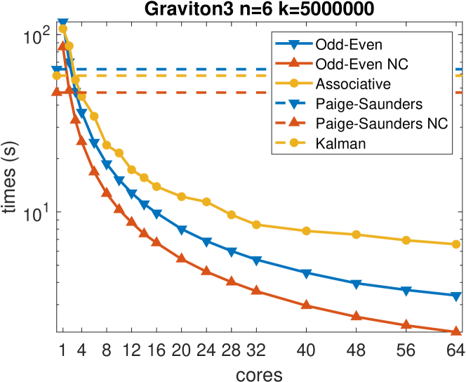
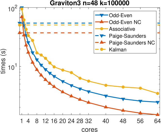
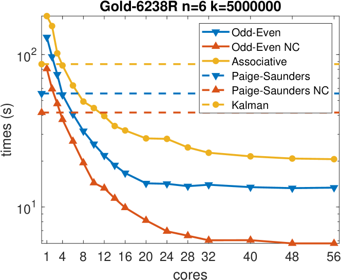
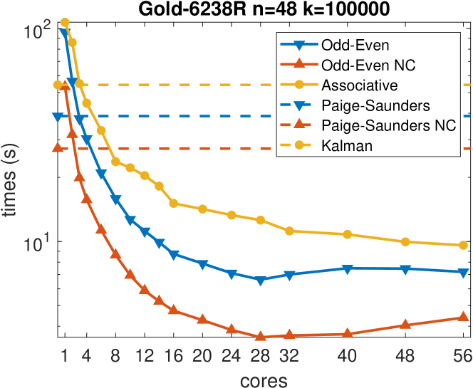
Figure 2: Running Times of all the smoothers on a server with 64 physical cores (Graviton3) and on a server with 56 physical cores (2 Intel Xeon Gold 6238R CPUs).

5.1 Implementation

We implemented all the algorithms that we described, including one of the sequential baseline algorithms, in both Matlab and C, using double-precision (64-bit) floating-point arithmetic. The implementation is based on the UltimateKalman implementation of the sequential Paige-Saunders algorithm [8] and uses its API. We only report on the performance of the C codes. We implemented the parallel algorithms using the open-source threading building blocks (TBB) library [17]. All the $\Theta(n^{3})$ matrix operations (matrix multiplications, factorizations, etc) are implemented using calls to a high-performance linear algebra library through the standard BLAS and LAPACK interfaces.

TBB is a C++ library designed to enable the implementation of shared-memory multi-core algorithms. It consists of a randomized work-stealing scheduler, a scalable memory allocator, as well as many convenience routines [17]. The scheduler is based on the Cilk scheduler and it provides similar theoretical guarantees [18, 19]. We chose to implement the algorithm with TBB for several reasons: (1) the theoretical performance guarantees, (2) the use of a library rather than a compiler-based parallel programming language reduces the risk of obsolescence and improves portability, (3) TBB, like Cilk, supports nested parallelism, which allows parallelism to be exploited at both the top parallel-in-time level and at the linear-algebra level below.

Our implementations consist almost entirely of C code. We use a single small C++ source file that contains two C-callable C++ functions. One of these functions invokes the tbb::parallel_for template function, while the other invokes tbb::parallel_scan. These functions also instructs TBB to use a certain number of cores (operating system threads) and to use a particular block size, the number of iterations or data items that are performed sequentially to reduce scheduling overheads. We use a block size of 10 unless noted otherwise.

Since it is impossible to restrict TBB to use only a single core (the restriction mechanism works for 2 cores and up), we also compile a sequential version of each parallel algorithm. This version replaces the calls to tbb::parallel_for and tbb::parallel_scan with simple C loops that perform the same computation sequentially. These versions also skip other parallel overheads, in particular the concurrent set operations that we use to ensure that all the memory allocated within tbb::parallel_scan is released.

Our test programs use TBB’s scalable memory allocator, not the memory allocator of the C library. This is done by linking them with a proxy library, libtbbmalloc_proxy that implements all the C and C++ memory management functionality. In parallel codes we align allocated memory regions to cache lines (64-bytes) using the posix_memalign alternative to malloc, to avoid false sharing.

5.2 Benchmark Problems

We tested the algorithms on synthetic problems with fixed $n_{i}$ and $m_{i}$ and with random fixed orthonormal $F_{i}$ and $G_{i}$ and with $H_{i}=I$. The observations $o_{i}$ were also random. We set $L_{i}=I$ and $K_{i}=I$. The use of orthonormal $F_{i}$ and $G_{i}$ avoids growth or shrinkage of the state vectors and hence overflows and underflows. We used two typical state-vector dimensions, either $n_{i}=m_{i}=6$ or $n_{i}=m_{i}=48$. One particular test, designed to clarify a specific hypothesis, used $n_{i}=m_{i}=500$. We denote the common dimension of the state by $n$.

Running times of the parallel algorithms do not include the time to build the array of steps, since in a parallel application, the array would typically be constructed using parallel input-output mechanisms (if the data is stored in files), using a parallel simulation code, or using an outer nonlinear Gauss-Newton-type solver, as explained in Section 3.2. In all cases, parallelizing these computations is clearly outside the scope of this article.

 
     

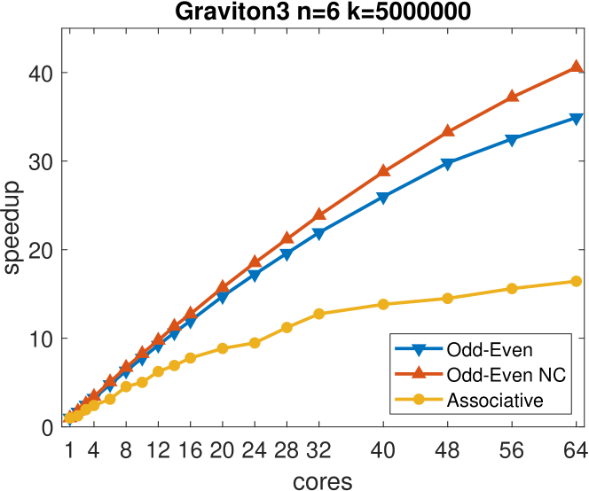
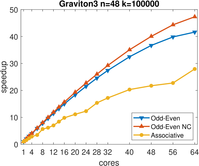
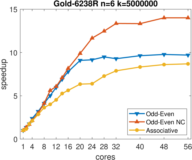
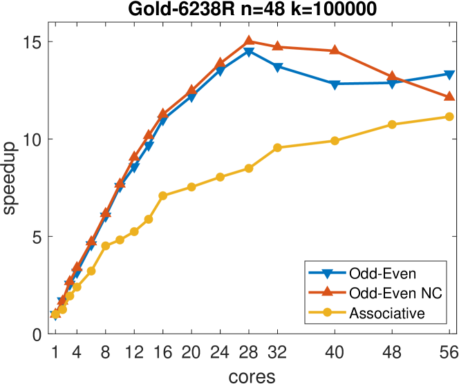
Figure 3: Speedups of the parallel smoothers . The ratios are relative to the running time of the same implementation on 1 core. The graphs are based on the same data shown in Figure 2.

5.3 Experimental Platforms

We evaluated the algorithms on several multi-core shared-memory servers. One has a Amazon Graviton3 CPU with 64 ARM cores running at 2.6 GHz and 128 GB of RAM (AWS EC2 c7g.metal instance; this instance runs directly on the hardware, with no virtualization). The second has two Intel Xeon Gold 6238R CPUs running at 2.2 GHz and 200 GB of DRAM. Each CPU has 28 physical cores for a total of 56. We also performed the experiments on a server with two older Intel Xeon CPUs, model E5-2699v3 with 18 physical cores each running at 2.30GHz. The results are similar to those on the Intel Xeon Gold 6238R server and are not shown.

We used GCC (version 7.5.0 on Intel servers and version 13.3 on ARM) and Intel’s threading building blocks, also known as TBB (version 2024.1 on Intel servers and 2021.11 on ARM). We used vendor-optimized BLAS and LAPACK libraries, MKL version 2024.1 on Intel servers and ARM Performance Libraries version 24.10 on the ARM server. Unless otherwise noted, we used the single-threaded (and thread-safe) version of the BLAS and LAPACK libraries.

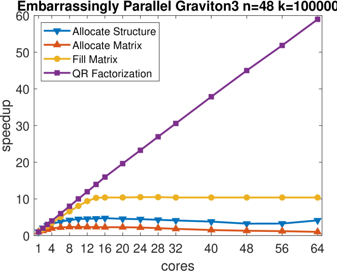
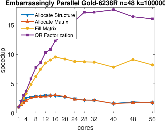
Figure 4: Speedups of 4 phases of a representative but embarrassingly-parallel micro-benchmark.

To characterize the capabilities of the hardware and of TBB, we implemented a simple embarrassingly-parallel micro-benchmark whose 4 phases characterize building blocks of our algorithms. In the first phase, the code allocates $k$ structures that represent steps and stores their addresses into an array. Next, for every step the algorithm allocates a $2n$-by-$n$ matrix and stores its address in the step structure. In the third phase, the code fills every matrix $A$ with values $A_{ij}=i+j$. Finally, the code computes the QR factorization of each matrix. Each phase is implemented with a separate tbb::parallel_for. The block size is 8 to avoid false sharing in phase 1. The speedups, shown in Figure 4 for $n=48$, indicate that speedups on QR factorization at this size excellent on the ARM server (59x on 64 cores; almost the same for $n=6$) but the memory-allocation and memory-filling phases do not scale well. On the Intel server speedups in the QR phase are limited to about 18 (and can be achieved with a single CPU). On both servers, the memory allocation phases scale poorly in spite of TBB’s scalable allocator, but their running times are fairly insignificant.

5.4 Results

The running times of the linear Kalman smoothers are shown in Figure 2 (all running times are medians of 5 runs) and the speedups of the parallel smoothers are shown in Figure 3. Figure 2 shows the running time of our new parallel algorithm, denoted Odd-Even, of the Särkkä & García-Fernández algorithm, denoted Associative, as well as of a conventional Kalman (RTS) smoother and of an implementation of the Paige-Saunders sequential QR-based algorithm. The conventional Kalman smoother and the parallel Associative smoother compute the smoothed states and their covariance matrices together; they cannot compute one without the other. In the Paige-Saunders algorithm and in our Odd-Even parallel algorithm, the evaluation of the covariance matrices of the smoothed states is a separate phase that we can skip, and we did evaluate the performance without this phase. This is denoted in the graphs by NC (no covariance). The NC variants are optimized for use in Levenberg-Marquardt-based nonlinear Kalman smoothing [15].

We can draw several conclusions from this data. First, all the parallel smoothers have a considerable overhead on one core. The parallel Odd-Even algorithm is about 1.8–2.5 times slower than the sequential Paige-Saunders algorithm (1.8–2.0 when covariance matrices are not computed). The overhead of the Associative parallel algorithm relative to a conventional Kalman smoother is similar, about 1.8–2.7.

Second, the Odd-Even parallel smoother is faster than the Associative Kalman smoother (except sometimes on 1 core only).

Third, the parallel algorithms do speed up and all of them easily beat the sequential variants. The Odd-Even smoother exhibits better speedups than the Associative one. On the ARM server performance improves monotonically and appreciably with the number of cores. On the Intel server, performance improves up to about 28 cores (one CPU) and mostly stagnates beyond that.

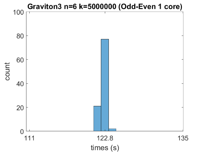
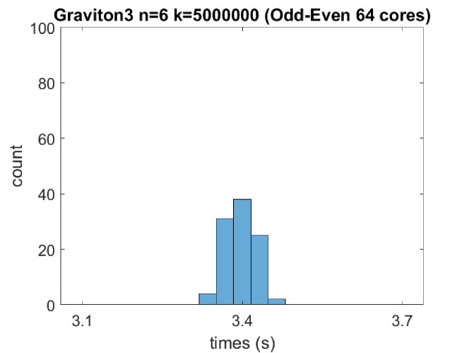
Figure 5: Running times distributions of the Odd-Even algorithm on 1 core and on 28 cores. The histograms analyze 100 runs each. The horizontal spans are set to 20% of the median running time.

Figure 5 shows the relatively small effect of the randomized work-stealing scheduler on the running time. Both histograms display the distribution of 100 running times; the horizontal span in both histograms is set to 20% of the median running time. With 64 cores, we observe running-time variations of up to $\pm$2.4% of the median running time. On 1 core the TBB scheduler was not invoked at all and the maximum variation is smaller, less than 0.9%. On the Intel Xeon server, the variation with 28 cores is 13% of the median running time and with 1 core only 1.5% (the graphs are omitted).

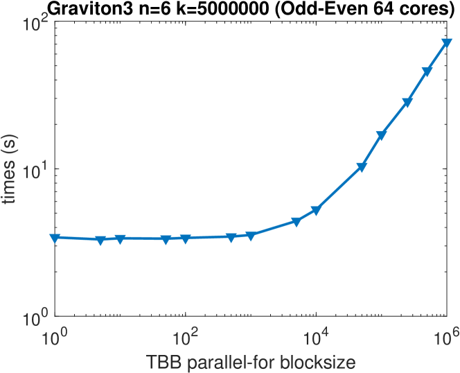
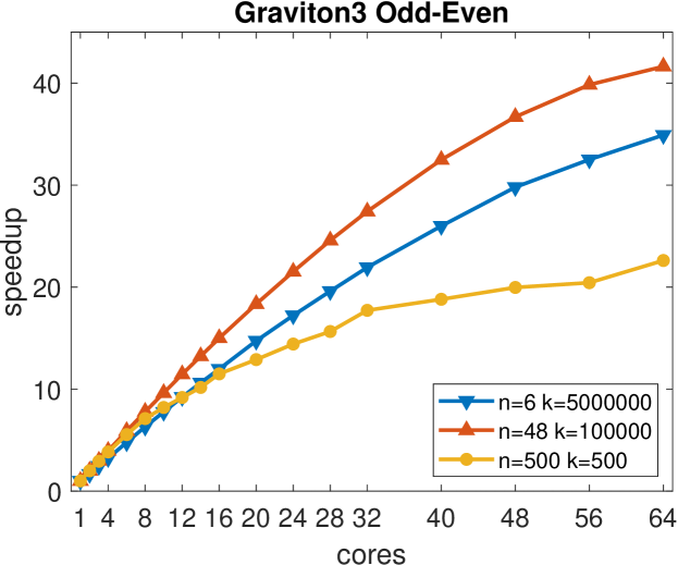
Figure 6: Left: Running times of the Odd-Even algorithm on 64 cores as a function of the block-size parameter in invocations of tbb::parallel_for loops. Right: Speedups of the of the Odd-Even algorithm problem of different dimensions, with a TBB block size of 10 for $n=6$ and $n=48$ and with a block size of 1 for $n=500$.

The graph in Figure 6 (left) shows the effect of the block-size parameter in invocations of tbb::parallel_for loops. The graph shows that even for small dimensions ($n_{i}=6$), performance remains roughly same with block sizes ranging from 1,000 all the way down to 1. At block sizes between 5,000 and 1,000,000, the smoother does slow down due to insufficient parallelism, as expected.

The graph in Figure 6 (right) shows what limits scalability on different problem sizes. The speedups on a problem with $n=48$ are somewhat better than with $n=6$. This is most likely caused by the better computation-to-communication ratio at $n=48$. On an even larger state dimension $n=500$ but a smaller number of steps $k=500$, the speedups are worse than the other two cases, most likely due to insufficient parallelism.

6 Conclusions

The parallel odd-even linear Kalman smoother that we introduced in this article offers best-in-class performance along with functionality not available until now in a parallel algorithm. Given enough cores our new parallel algorithm outperforms all sequential Kalman smoothers, in spite of its additional arithmetic overhead. The algorithm also outperforms the only other parallel-in-time Kalman smoother [3].

The core of the new algorithm is a specialized QR factorization. The use of this framework, introduced by Paige and Saunders [12], contributes to the functionality of the smoother in several ways.

First, the algorithm is conditionally backward stable. The backward stability depends (only) on the input covariance matrices, the $K_{i}$ and $L_{i}$ matrices, just like the stability of the Paige-Saunders algorithm. In particular, when these matrices are either diagonal, a common case, or well conditioned, the overall algorithm is backward stable. In contrast, nothing is known about the numerical stability of the only other parallel-in-time Kalman smoother [3].

Second, the algorithm can handle problems in which the expectation of the initial state is not known. This is a fairly common case that arises, for example, in inertial navigation. Our algorithm can also handle cases where $H_{i}\neq I$. The Särkkä and García-Fernández smoother [3] cannot handle such problems, but unlike ours, it can handle problems with singular input covariance matrices, just like the conventional Kalman (RTS) smoother.

Third, the covariance matrices of the smoothed state estimates are computed in a distinct final phase. Our implementation can skip this phase, speeding up the computation when these covariance matrices are not needed, which is the case in a Levenberg-Marquart nonlinear Kalman smoother [15]. The Särkkä and García-Fernández smoother must compute the covariance matrices, just like conventional Kalman smoothers, so it cannot benefit from this optimization.

Another key contribution of this article is the discovery that the SelInv algorithm [6] can be used to compute the covariance matrices of the smoothed estimates. This discovery also applies to the Paige-Saunders algorithm, where SelInv can replace a sequence of orthogonal transformations, but it is particularly crucial for the odd-even parallel algorithm, because there is no apparent way to extend the Paige-Saunders approach to this case.

The final contribution of this paper is the parallel implementation of the Särkkä and García-Fernández smoother, which to the best of our knowledge is the first (it appears that the implementation described in their article [3] is sequential; it was used to test correctness and to evaluate the work and critical path using sequential runs).

We do acknowledge one limitation of the algorithms (both ours and that of Särkkä and García-Fernández): due to the arithmetic (work) overheads of the parallel algorithms, the sequential variants are faster on small number of cores. Since parallelizing the operations of each step in a sequential-in-time algorithm appears to be effective only in very high dimensions [16], developing low-overhead parallel-in-time smoothers appears to be an important open challenge.

We also acknowledge that both families of algorithms exhibit limited strong scaling; the data in Figure 4 suggests that this is mostly due to memory-bandwidth and cache misses, but also that it might be possible to further improve performance.

Finally, it is evident from the structure of $UA$ that $(UA)^{T}(UA)$, the coefficient matrix of the normal equations of the linear least-squares problem, is block tridiagonal. Therefore, the normal equations can be solved in parallel using block odd-even reduction of this block tridiagonal matrix [4, 5], yielding a third parallel algorithm for Kalman smoothing. However, this approach is unstable and does not appear to have any advantage over our new algorithm.

Our implementations are available at https://github.com/sivantoledo/ultimate-kalman under standard open-source licenses.

Acknowledgments. We thank the reviewers for comments and suggestions that helped improve the article. This research was supported in part by grant 1919/19 from the Israel Science Foundation.

References

- [1] R. E. Kalman, “A new approach to linear filtering and prediction problems,” Journal of Basic Engineering, vol. 82, no. 1, pp. 35–45, 1960.
- [2] H. E. Rauch, F. Tung, and C. T. Striebel, “Maximum likelihood estimates of linear dynamic systems,” AIAA Journal, vol. 3, no. 8, pp. 1445–1450, 1965.
- [3] S. Särkkä and Á. F. García-Fernández, “Temporal parallelization of Bayesian smoothers,” IEEE Transactions on Automatic Control, vol. 66, no. 1, pp. 299–306, 2021.
- [4] B. L. Buzbee, G. H. Golub, and C. W. Nielson, “On direct methods for solving Poisson’s equations,” SIAM Journal on Numerical Analysis, vol. 7, no. 4, pp. 627–656, 1970.
- [5] D. Heller, “Some aspects of the cyclic reduction algorithm for block tridiagonal linear systems,” SIAM Journal on Numerical Analysis, vol. 13, no. 4, pp. 484–496, 1976.
- [6] L. Lin, C. Yang, J. C. Meza, J. Lu, L. Ying, and W. E, “SelInv—an algorithm for selected inversion of a sparse symmetric matrix,” ACM Transactions on Mathematical Software, vol. 37, no. 4, 2011.
- [7] S. Särkkä and L. Svensson, Bayesian Filtering and Smoothing. Cambridge University Press, 2023.
- [8] S. Toledo, “Algorithm 1051: UltimateKalman, flexible Kalman filtering and smoothing using orthogonal transformations,” ACM Transactions on Mathematical Software, vol. 50, no. 4, pp. 1–19, 2024.
- [9] T. Kailath, A. H. Sayed, and B. Hassibi, Linear Estimation. Prentice Hall, 2000.
- [10] J. Humpherys, P. Redd, and J. West, “A fresh look at the Kalman filter,” SIAM Review, vol. 54, no. 4, pp. 801–823, 2012.
- [11] D. B. Duncan and S. D. Horn, “Linear dynamic recursive estimation from the viewpoint of regression analysis,” Journal of the American Statistical Association, vol. 67, no. 340, pp. 815–821, 1972.
- [12] C. C. Paige and M. A. Saunders, “Least squares estimation of discrete linear dynamic systems using orthogonal transformations,” SIAM Journal on Numerical Analysis, vol. 14, no. 2, pp. 180–193, 1977.
- [13] Å. Björck, Numerical Methods for Least Squares Problems, 2nd ed. Philadelphia, PA, USA: SIAM, 2024.
- [14] B. M. Bell, “The iterated Kalman smoother as a Gauss-Newton method,” SIAM Journal on Optimization, vol. 4, no. 3, pp. 626–636, 1994.
- [15] S. Särkkä and L. Svensson, “Levenberg-Marquardt and line-search extended Kalman smoothers,” in Proceedings of the IEEE International Conference on Acoustics, Speech and Signal Processing (ICASSP), 2020, pp. 5875–5879.
- [16] O. Rosen and A. Medvedev, “Efficient parallel implementation of state estimation algorithms on multicore platforms,” IEEE Transactions on Control Systems Technology, vol. 21, no. 1, pp. 107–120, 2013.
- [17] A. Kukanov and M. J. Voss, “The foundations for scalable multi-core software in Intel Threading Building Blocks,” Intel Technology Journal, vol. 11, pp. 309–322, 2007.
- [18] R. D. Blumofe and C. E. Leiserson, “Scheduling multithreaded computations by work stealing,” in Proceedings 35th Annual Symposium on Foundations of Computer Science (FOCS), 1994, pp. 356–368.
- [19] R. D. Blumofe, C. F. Joerg, B. C. Kuszmaul, C. E. Leiserson, K. H. Randall, and Y. Zhou, “Cilk: an efficient multithreaded runtime system,” SIGPLAN Notices, vol. 30, no. 8, pp. 207–216, Aug. 1995.