Double Momentum and Error Feedback for Clipping with
Fast Rates and Differential Privacy
 

Abstract

Strong Differential Privacy (DP) and Optimization guarantees are two desirable properties for a method in Federated Learning (FL). However, existing algorithms do not achieve both properties at once: they either have optimal DP guarantees but rely on restrictive assumptions such as bounded gradients/bounded data heterogeneity, or they ensure strong optimization performance but lack DP guarantees. To address this gap in the literature, we propose and analyze a new method called Clip21-SGD2M based on a novel combination of clipping, heavy-ball momentum, and Error Feedback. In particular, for non-convex smooth distributed problems with clients having arbitrarily heterogeneous data, we prove that Clip21-SGD2M has optimal convergence rate and also near optimal (local-)DP neighborhood. Our numerical experiments on non-convex logistic regression and training of neural networks highlight the superiority of Clip21-SGD2M over baselines in terms of the optimization performance for a given DP-budget.

1 Introduction

Federated Learning (Konečný et al., 2016; McMahan et al., 2017a) is a modern training paradigm where multiple (possibly heterogeneous) clients aim to jointly train a machine learning model without sacrificing the privacy of their own data. This setup presents several noticeable challenges in terms of algorithm design affecting different aspects of training, including communication efficiency, partial participation of clients, data heterogeneity, security, and privacy (Kairouz et al., 2021; Wang et al., 2021). As a result, numerous optimization methods for Federated Learning (FL) have been introduced in recent years. However, despite extensive research in the field, achieving both strong optimization convergence and robust differential privacy (DP) guarantees (Dwork et al., 2014) simultaneously in an FL algorithm remains challenging due to the conflicting nature of these objectives. Indeed, most of the results in the field of DP are obtained by adding noise (e.g. Gaussian noise) to the method’s update (Abadi et al., 2016; Chen et al., 2020) in order to protect the client’s data that could be potentially reconstructed from the updates. Unfortunately, this approach results in less accurate updates, which negatively affects the convergence. Moreover, to ensure DP, this mechanism should be applied to the method with bounded updates, which is typically achieved via gradient clipping (Pascanu et al., 2013).

Further complicating the issue, naïve distributed Clipped Gradient Descent (Clip-GD) is not guaranteed to converge (Khirirat et al., 2023) when clients have heterogeneous data (even in the absence of any additive DP-noise), which is a common scenario in FL. To address this issue, Khirirat et al. (2023) apply the EF21 mechanism – originally developed by Richtárik et al. (2021) for contractive compression operators to improve the standard Error Feedback (Seide et al., 2014) – to Clip-GD, resulting in a method known as Clip21-GD. Khirirat et al. (2023) show that in contrast to Clip-GD, Clip21-GD converges with $\mathcal{O}(\nicefrac{{1}}{{T}})$ rate for smooth non-convex problems with arbitrary heterogeneous data on clients. However, their analysis is limited to the case of full-batched gradients and does not work with DP-noise. This leads us to the natural question:

Is it possible to design a method that combines both strong optimization performance and

DP guarantees in a stochastic setting?

Our contribution.

In this paper, we provide a positive answer to the above question by introducing a new method, named Clip21-SGD2M, which incorporates clipping, error feedback and heavy-ball momentum (Polyak, 1964) in a novel way. For smooth non-convex distributed optimization problems, we show that Clip21-SGD2M (i) converges with optimal $\mathcal{O}(\nicefrac{{1}}{{T}})$ rate when the workers compute full gradients, (ii) converges with optimal $\widetilde{\mathcal{O}}(\nicefrac{{1}}{{\sqrt{nT}}})$ high-probability convergence rate when the workers use stochastic gradients with sub-Gaussian noise, and (iii) has near optimal local DP-error when DP-noise is added to the clients’ updates. We also prove that Clip21-SGD is not guaranteed to converge in the stochastic case, underscoring the need for changes in the algorithm. Our experiments on logistic regression and neural networks highlight the robustness of Clip21-SGD2M to the choice of clipping level and indicate Clip21-SGD2M’s superiority over Clip-SGD and Clip21-SGD in terms of optimization performance for a given DP-budget.

1.1 Problem Formulation and Assumptions

We consider the optimization problem of the form

$$\min\limits_{x\in\mathbb{R}^{d}}\left[f(x)\coloneqq\frac{1}{n}\sum_{i=1}^{n}f_{i}(x)\right]$$ (1)

that typically appears in many machine learning applications and is standard for Federated Learning. Here $x$ denotes the parameters of a model, $f_{i}$ represents the loss associated with the local dataset $\mathcal{D}_{i}$ of worker $i\in[n]$, and $f$ is an average loss across all workers participating in the training process.

We make two main assumptions on the problem. The first one is smoothness, which is standard for non-convex optimization (Carmon et al., 2020; Danilova et al., 2022). In addition, we also assume that $f(x)$ is uniformly lower bounded since otherwise, problem (1) is intractable.

Assumption 1.

We assume that each individual loss function $f_{i}$ is $L$-smooth, i.e., for any $x,y\in\mathbb{R}^{d}$ and $i\in[n]$ we have

$$\|\nabla f_{i}(x)-\nabla f_{i}(y)\|\leq L\|x-y\|.$$ (2)

Moreover, we assume that $f^{*}\coloneqq\inf_{x\in\mathbb{R}^{d}}f(x)>-\infty$.

We also note that our analysis can be easily generalized to the case when $L$ depends on $f_{i}$.

Next, since computation of the full gradients is expensive in many practical applications, it is natural to consider the case when clients compute stochastic gradients. We make the following assumption on the stochastic noise of these gradients.

Assumption 2.

We assume that each worker $i$ has access to a $\sigma$-sub-Gaussian unbiased estimator $\nabla f_{i}(x,\xi)$ of a local gradient $\nabla f_{i}(x)$, i.e., for some $\sigma\geq 0$ and any $x\in\mathbb{R}^{d}$ and $\forall i\in[n]$ we have

$$\hskip-5.0pt\mathbb{E}\left[\nabla f_{i}(x,\xi)\right]=\nabla f_{i}(x),\mathbb{E}\left[\exp\left(\nicefrac{{\|\theta_{i}^{t}\|^{2}}}{{\sigma^{2}}}\right)\right]\leq\exp(1),$$ (3)

where $\xi$ denotes the source of the stochasticity and $\theta_{i}\coloneqq\nabla f_{i}(x,\xi)-\nabla f_{i}(x)$.

Although this assumption is stronger than bounded variance, it is standard for the high-probability analysis of SGD-type methods with polylogarithmic dependence on the confidence level (Nemirovski et al., 2009; Ghadimi and Lan, 2012). The second part of (3) is equivalent to $\Pr\left(\|\theta^{t}_{i}\|\geq b\right)\leq 2\exp\left(-\nicefrac{{b^{2}}}{{(2\sigma^{2})}}\right)$ up to a constant factor in $\sigma^{2}$ (Vershynin, 2018). We also note that it is possible to show high-probability bounds for SGD-type methods with polylogarithmic dependence on the confidence level when the noise has sub-Weibull tails (Madden et al., 2024), i.e., the noise can be even heavier but it affects the polylogarithmic factors.

Finally, we provide two important definitions for this work. The first one is the definition of the clipping operator, which is a non-linear map from $\mathbb{R}^{d}$ to $\mathbb{R}^{d}$ parameterized by the clipping threshold/level $\tau>0$ and defined as

$$\operatorname{clip}_{\tau}(x)\coloneqq\begin{cases}\frac{\tau}{\|x\|}x,&\text{ if }\|x\|>\tau,\\ x,&\text{ if }\|x\|\leq\tau.\end{cases}$$ (4)

Next, we will use the following classical definition of $(\varepsilon,\delta)$-Differential Privacy, which introduces plausible deniability into the output of a learning algorithm.

Definition 1 ($(\varepsilon,\delta)$-Differential Privacy (Dwork et al., 2014)).

A randomized method $\mathcal{M}:\mathcal{D}\to\mathcal{R}$ satisfies $(\varepsilon,\delta)$-Differential Privacy ($(\varepsilon,\delta)$-DP) if for any adjacent $D,D^{\prime}\in\mathcal{D}$ (e.g., if $D$ and $D^{\prime}$ are datasets, then the adjacency means that $D$ and $D^{\prime}$ differ in $1$ sample) and for any $S\subseteq\mathcal{R}$

$$\Pr\left(\mathcal{M}(D)\in S\right)\leq e^{\varepsilon}\Pr\left(\mathcal{M}(D^{\prime})\in S\right)+\delta.$$ (5)

In this definition, the smaller $\varepsilon,\delta$ are, the more private the method is. Intuitively, if inequality (5) holds with small values of $\varepsilon$ and $\delta$, it becomes difficult to infer the specific data point that differs between two similar datasets based solely on the output of $\mathcal{M}$.

1.2 Related Work

Differential Privacy.

The most common approach to obtaining DP guarantees is to clip each client’s update, i.e., by bounding their $\ell_{2}$ norm, and adding a calibrated amount of Gaussian noise to each update or the average. This is typically sufficient to obscure the influence of any single client (McMahan et al., 2017b). Commonly, two scenarios of the DP model are considered: the central model and the local model. In the first setting, central privacy, a trusted server collects updates and adds noise only before updating the server-side model. This ensures that client data remains private from external parties. In the second setting, local privacy, client data is protected even from the server by clipping and adding noise to updates locally before sending them to the server, ensuring privacy from both the server and other clients (Kasiviswanathan et al., 2011; Allouah et al., 2024). The local privacy setting offers stronger privacy against untrusted servers but results in poorer learning performance due to the need for more noise to obscure individual updates (Chan et al., 2012; Duchi et al., 2018). This can be improved by using a secure shuffler (Erlingsson et al., 2019; Balle et al., 2019), which permutes updates, or a secure aggregator (Bonawitz et al., 2017), which sums updates before sending them to the server. These methods anonymize updates and enhance privacy while maintaining reasonable learning performance, even without a fully trusted server. Finally, (Chaudhuri et al., 2022; Hegazy et al., 2024) show that when DP is required, one can also achieve compression of updates for free.

In this work, we adopt the local DP model by injecting Gaussian noise into each client’s update. However, the average noise can also be viewed as noise added to the average update. Therefore, Clip21-SGD2M is compatible with all the aforementioned techniques and can also be applied to the central DP model with a smaller amount of noise.

Distributed methods with clipping.

In the single-node regime, Clip-SGD has been analyzed under various assumptions by many authors (Zhang et al., 2020b, c, a; Gorbunov et al., 2020a; Cutkosky and Mehta, 2021; Sadiev et al., 2023; Liu et al., 2023). Of course, these results can be generalized to the multi-node case if clipping is applied to the aggregated (e.g. averaged) vector, although mini-batching requires a refined analysis when the noise is heavy-tailed(Kornilov et al., 2024). However, to get DP, clipping has to be applied to the vectors communicated by clients to the server. In this regime, Clip-SGD is not guaranteed to converge even without any stochastic noise in the gradients (Chen et al., 2020; Khirirat et al., 2023). There exist several approaches to bypass this limitation that can be split into two lines of work. The first one relies on explicit or implicit assumptions about bounded heterogeneity. More precisely, Liu et al. (2022) analyze a version of Local-SGD/FedAvg (Mangasarian, 1995; McMahan et al., 2017a) with gradient clipping for homogeneous data case assuming that the stochastic gradients have symmetric distribution around their mean and Wei et al. (2020) consider Local-SGD with clipping of the models and analyze its convergence under bounded heterogeneity assumption. Moreover, the boundedness of the stochastic gradient is another assumption used in the literature but it implies the boundedness of gradients’ heterogeneity of clients as well. This assumption is used in numerous works, including: i) Zhang et al. (2022) in the analysis of a version of FedAvg with clipping of model difference (also empirically studied by Geyer et al. (2017)), ii) Noble et al. (2022) who propose and analyze a version of SCAFFOLD (Karimireddy et al., 2020) with gradient clipping (DP-SCAFFOLD), iii) Li and Chi (2023) who propose and analyze a version of BEER (Li et al., 2021) with gradient clipping (PORTER) under bounded gradient and/or bounded data heterogeneity assumption, and iv) Allouah et al. (2024) who study a version of Gossip-SGD (Nedic and Ozdaglar, 2009) with gradient clipping (DECOR). Although most of the mentioned works have rigorous DP guarantees, the corresponding methods are not guaranteed to converge for arbitrary heterogeneous problems.

The second line of work focuses on the clipping of shifted (stochastic) gradient. In particular, Khirirat et al. (2023) proposed and analyzed Clip21-GD, which is based on the application of EF21 (Richtárik et al., 2021) to the clipping operator, and Gorbunov et al. (2024) develop and analyze methods that apply clipping to the difference of stochastic gradients and learnable shift – an idea that was initially proposed by Mishchenko et al. (2019) to handle data heterogeneity in the Distributed Learning with unbiased communication compression. However, the analysis from (Khirirat et al., 2023) is limited to the noiseless regime, i.e., full-batched gradients are computed on workers, and both of the mentioned works do not provide DP guarantees. We also note that clipping of gradient differences is helpful in tolerating Byzantine attacks in the partial participation regime (Malinovsky et al., 2023).

Error Feedback.

Error Feedback (EF) (Seide et al., 2014) is a popular technique for incorporating communication compression into Distributed/Federated Learning. However, for non-convex smooth problems, the existing analysis of EF is provided either for the single-node case or relies on restrictive assumptions such as boundedness of the gradient/compression error or boundedness of the data heterogeneity (gradient dissimilarity) (Stich et al., 2018; Stich and Karimireddy, 2019; Karimireddy et al., 2019; Koloskova et al., 2019; Beznosikov et al., 2023; Tang et al., 2019; Xie et al., 2020; Sahu et al., 2021). Moreover, the convergence bounds for EF also depend on the data heterogeneity, which is not an artifact of the analysis as illustrated in the experiments on strongly convex problems Gorbunov et al. (2020b). Richtárik et al. (2021) address this limitation and propose a new version of Error Feedback called EF21. However, the existing analysis of EF21-SGD requires the usage of large batch sizes to achieve any predefined accuracy (Fatkhullin et al., 2021). It turns out that the large batch size requirement is unavoidable for EF21-SGD to converge, but this issue can be fixed using momentum (Fatkhullin et al., 2024). Momentum is also helpful in the decentralized extensions of Error Feedback (Yau and Wai, 2022; Huang et al., 2023; Islamov et al., 2024a).

2 Non-Convergence of Clip-SGD and Clip21-SGD

We start with a discussion of the key limitation of Clip-SGD (Algortihm 1) and Clip21-SGD (Algorithm 2) – their potential non-convergence.

Algorithm 1 Clip-SGD (Abadi et al., 2016)

1:$x^{0}\in\mathbb{R}^{d}$, stepsize $\gamma>0$, clipping parameter $\tau>0$

2:for $t=0,\ldots,T-1$ do

3:  for $i=1,\dots,n$ in parallel do

4:   $g_{i}^{t}=\operatorname{clip}_{\tau}(\nabla f_{i}(x^{t},\xi_{i}^{t}))$

5:  end for

6:  $g^{t}=\frac{1}{n}\sum_{i=1}^{n}g_{i}^{t}$

7:  $x^{t+1}=x^{t}-\gamma g^{t}$

8:end for

We start by restating the example from (Chen et al., 2020) illustrating the potential non-convergence of Clip-SGD even when full gradients are computed on clients (Clip-GD).

Example 1 (Non-Convergence of Clip-GD (Chen et al., 2020)).

Let $n=2$, $d=1$, and $f_{1}(x)=\frac{1}{2}(x-3)^{2}$, $f_{2}(x)=\frac{1}{2}(x+3)^{2}$ in problem (1) having a unique solution $x^{*}=0$. Consider Clip-GD with $\tau=1$ applied to this problem. If for some $t_{0}$ we have $x^{t_{0}}\in[-2,2]$ in Clip-GD, then $g^{t}=0$ and $x^{t}=x^{t_{0}}$ for any $t\geq t_{0}$, which can be seen via direct calculations. In particular, for any $x^{0}\in[-2,2],$ the method does not move away from $x^{0}$.

To address the non-convergence of Clip-GD, Khirirat et al. (2023) propose Clip21-GD that applies the clipping operator to the difference between $\nabla f_{i}(x^{t+1})$ and the shift $g_{i}^{t}$, which is designed to approximate $\nabla f_{i}(x^{t})$. In the deterministic case, this strategy ensures that after a certain number of steps, clipping turns off on all clients since $\|\nabla f_{i}(x^{t+1})-g_{i}^{t}\|$ becomes smaller than $\tau$ for all $i\in[n]$ eventually. However, when workers compute stochastic gradients instead of the full gradients, Clip21-SGD can be non-convergent as well. To illustrate this, we consider the ideal version of Clip21-SGD with stochastic gradients, i.e., instead of $g_{i}^{t}$, we use $\nabla f_{i}(x^{t+1})$ as a shift:

$$x^{t+1} =x^{t}-\gamma g^{t},\quad g^{t}=\frac{1}{n}\sum_{i=1}^{n}g_{i}^{t},$$ (6)

$$g_{i}^{t+1} =\nabla f_{i}(x^{t+1})+\operatorname{clip}_{\tau}(\nabla f_{i}(x^{t+1},\xi^{t+1}_{i})-\nabla f_{i}(x^{t+1})).$$

Algorithm 2 Clip21-SGD (Khirirat et al., 2023)

1:$x^{0},g^{0}\in\mathbb{R}^{d}$, stepsize $\gamma>0$, clipping parameter $\tau>0$, $g_{i}^{0}=g^{0}$ for all $i\in[n]$

2:for $t=0,\ldots,T-1$ do

3:  $x^{t+1}=x^{t}-\gamma g^{t}$

4:  for $i=1,\dots,n$ in parallel do

5:   $c_{i}^{t+1}=\operatorname{clip}_{\tau}(\nabla f_{i}(x^{t+1},\xi^{t+1}_{i})-g_{i}^{t})$

6:   $g_{i}^{t+1}=g_{i}^{t}+c_{i}^{t+1}$

7:  end for

8:  $g^{t+1}=g^{t}+\frac{1}{n}\sum_{i=1}^{n}c_{i}^{t+1}$

9:  

10:end for

The next theorem shows that even this (ideal) version of stochastic Clip21-SGD fails to converge even for a simple quadratic problem with sub-Gaussian noise.

Theorem 1.

Let $L,\sigma>0,$ $0<\gamma\leq 1/L,n=1$. There exists a convex, $L$-smooth problem, clipping parameter $\tau<\nicefrac{{3\sigma\sqrt{3}}}{{10}}$, and an unbiased stochastic gradient satisfying Assumption 2 such that the method (6) is run with a stepsize $\gamma$ and clipping parameter $\tau$, then for all $x^{0}\in\{(0,x_{(2)}^{0})\in\mathbb{R}^{2}\mid x_{(2)}^{0}<0\}$ we have

$$\mathbb{E}\left[\|\nabla f(x^{T})\|^{2}\right]\geq\frac{1}{2}\min\left\{\|\nabla f(x^{0})\|^{2},\frac{\tau^{2}}{45}\right\}.$$

Moreover, fix $0<\varepsilon<\nicefrac{{L}}{{\sqrt{2}}}$ and $x^{0}=(0,-1)^{\top}.$ Let the sub-Gaussian variance of stochastic gradients is bounded by $\nicefrac{{\sigma^{2}}}{{B}}$ where $B$ is a batch size. If $B<\nicefrac{{27\sigma^{2}}}{{(60\varepsilon^{2})}}$ and $\tau\geq\nicefrac{{\varepsilon}}{{(3\sqrt{10})}}$, then we have $\mathbb{E}\left[\|\nabla f(x^{T})\|^{2}\right]>\varepsilon^{2}$ for all $T>0.$

We also illustrate the above result with simple numerical experiments reported in Figure 1. The left figure shows that Clip21-SGD diverges from the initial function sub-optimality level while the right one demonstrates non-improvement with the number of workers $n$ — one of the desired properties of algorithms for FL.

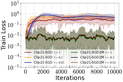
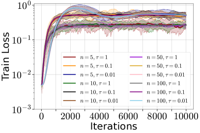
Figure 1: Left: behavior of stochastic Clip21-SGD and Clip21-SGD2M without DP noise (see Algorithm 3) initialized at $x^{0}=(0,-0.07)^{\top}$, with stepsize $\gamma=\nicefrac{{1}}{{\sqrt{T}}}$ where $T=10^{4}$, i.e., close to the solution and small stepsize. We observe that Clip21-SGD escapes the good neighborhood of the solution for the problem from Theorem 1 with $n=1,L=2,\sigma=5,$ and varying $\tau\in\{1,0.1,0.01\}.$ In contrast, Clip21-SGD2M remains stable around the solution. Right: convergence of Clip21-SGD does not improve with the increase of $n$ for the same problem.

3 Clip21-SGD2M: New Method and Theoretical Results

This section introduces Clip21-SGD2M (Algorithm 3), a novel distributed method with clipping that can be viewed as an enhanced version of Clip21-SGD, integrating momentum and DP-noise. That is, to control the noise coming from the stochastic gradients, we introduce momentum buffers $\{v_{i}^{t}\}_{i\in[n]}$ on the clients and clip $\{v_{i}^{t+1}-g_{i}^{t}\}_{i\in[n]}$ in contrast to the stochastic version of Clip21-SGD that applies clipping to potentially noisier vectors $\{\nabla f_{i}(x^{t+1},\xi_{i}^{t+1})-g_{i}^{t}\}_{i\in[n]}$. Moreover, similarly to Clip21-SGD – which can be seen as EF21 (Richtárik et al., 2021) where the compression operator is replaced with clipping – Clip21-SGD2M with $\hat{\beta}=1$ can also be interpreted as EF21M (Fatkhullin et al., 2024) with the same replacement. However, a crucial part of Clip21-SGD2M is the second momentum parameterized by $\hat{\beta}$. This is a key component of the method allowing it to control the DP-noise and preventing the method from the rapid accumulation of DP-noise in the update direction $g^{t}$. We note that the double-momentum in Clip21-SGD2M is noticeably different from the existing algorithmic ideas that are also called double-momentum. That is, in contrast to EF21-SGD2M from (Fatkhullin et al., 2024), we do not apply explicit momentum on the clients on top of the first one (this is why Clip21-SGD2M does not reduce to EF21-SGD2M when the clipping operator is formally replaced with the compression operator). Moreover, in contrast to $\mu^{2}$-SGD from (Levy, 2023), Clip21-SGD2M does not use iterates averaging and STORM-like estimator (Cutkosky and Orabona, 2019), and, unlike AdEMAMix (Pagliardini et al., 2024), Clip21-SGD2M does not use a mixture of two momentum buffers. The reason why we say that Clip21-SGD2M has double momentum can be explained as follows: if $\sigma_{\omega}=0$ (no DP-noise), $\beta=1$ (the first momentum is “turned off”), and $\tau=\infty$ (no clipping), then $g^{t+1}=(1-\hat{\beta})g^{t}+\frac{\hat{\beta}}{n}\sum_{i=1}^{n}\nabla f_{i}(x^{t+1},\xi_{i}^{t+1})$, i.e., the method reduces to the standard SGD with the heavy-ball momentum (Polyak, 1964).

Next, both EF21 and EF21M rely on the contractiveness property of the compression operator $\mathcal{C}(x)$, i.e., the (randomized) mapping $\mathcal{C}:\mathbb{R}^{d}\to\mathbb{R}^{d}$ should satisfy

$$\mathbb{E}\left[\|\mathcal{C}(x)-x\|^{2}\right]\leq(1-\nu)\|x\|^{2}\text{ for some }\nu\in(0,1],$$ (7)

where the expectation is w.r.t. the randomness of $\mathcal{C}$. As shown and discussed by Khirirat et al. (2023), clipping satisfies a condition that resembles (7) namely

$$\|\operatorname{clip}_{\tau}(x)-x\|^{2}\leq\begin{cases}0,&\text{if }\|x\|\leq\tau,\\ \left(1-\frac{\tau}{\|x\|}\right)^{2}\|x\|^{2},&\text{if }\|x\|>\tau,\end{cases}$$ (8)

but there is a significant difference: if $\|x\|>\tau$, the contraction factor depends on $x$ and can be arbitrarily close to $1$. To circumvent this issue, Khirirat et al. (2023) prove via induction that for all iterates of Clip21-GD, the vectors $\nabla f_{i}(x^{t+1})-g_{i}^{t}$ have norms bounded by some constant depending on the starting point. We show that a similar statement holds for Clip21-SGD2M when the clients compute full-batch gradients and no DP-noise is added, and we start our analysis with this important case. We also present the results in the stochastic case with and without DP noise.

Algorithm 3 Clip21-SGD2M

1:$x^{0},g^{0},v^{0}\in\mathbb{R}^{d}$ (by default $g^{0}=v^{0}=0$), momentum parameters $\beta,\hat{\beta}\in(0,1],$ stepsize $\gamma>0,$ clipping parameter $\tau>0$, DP-variance parameter $\sigma^{2}_{\omega}\geq 0$

2:Set $g_{i}^{0}=g^{0}$ and $v_{i}^{0}=v^{0}$ for all $i\in[n]$

3:for $t=0,\ldots,T-1$ do

4:  $x^{t+1}=x^{t}-\gamma g^{t}$

5:  for $i=1,\dots,n$ do

6:   $v_{i}^{t+1}=(1-\beta)v_{i}^{t}+\beta\nabla f_{i}(x^{t+1},\xi^{t+1}_{i})$

7:   $\omega_{i}^{t+1}\sim\mathcal{N}(0,\sigma^{2}_{\omega}\mathbf{I})$ only for DP version

8:   $c_{i}^{t+1}=\operatorname{clip}_{\tau}(v_{i}^{t+1}-g_{i}^{t})+$ $\omega_{i}^{t+1}$

9:   $g_{i}^{t+1}=g_{i}^{t}+\hat{\beta}\operatorname{clip}_{\tau}(v_{i}^{t+1}-g_{i}^{t})$

10:  end for

11:  $g^{t+1}=g^{t}+\frac{\hat{\beta}}{n}\sum_{i=1}^{n}c_{i}^{t+1}$

12:end for

3.1 Analysis in the Deterministic Case

The next result derives a convergence rate for Clip21-SGD2M when $\nabla f_{i}(x^{t+1},\xi^{t+1}_{i})\equiv\nabla f_{i}(x^{t})$ almost surely, i.e., Assumption 2 holds with $\sigma=0$.

Theorem 2 (Simplified).

Let Assumptions 1 and 2 with $\sigma=0$ hold. Let $B\coloneqq\max_{i}\|\nabla f_{i}(x^{0})\|>3\tau$ and $\Delta\geq f(x^{0})-f^{*}.$ Then, for any constant $\hat{\beta}\in(0,1]$, there exists a stepsize $\gamma\leq\min\{\nicefrac{{1}}{{12L}},\nicefrac{{\tau}}{{12BL}}\}$ and momentum parameter $\beta=4L\gamma$ such that the iterates of Clip21-SGD2M (Algorithm 3) converge with the rate

$$\frac{1}{T}\sum_{t=0}^{T-1}\|\nabla f(x^{t})\|^{2}\leq\mathcal{O}\left(\frac{L\Delta(1+\nicefrac{{B}}{{\tau}})}{T}\right).$$ (9)

Moreover, after at most $\frac{2B}{\hat{\beta}\tau}$ iterations, the clipping will eventually be turned off for all workers.

Proof sketch.

The proof of Theorem 2 (and all following ones) relies on a similar Lyapunov function that is used by Fatkhullin et al. (2024) in the analysis of EF21M:

$$\Phi^{t}\coloneqq f(x^{t})-f^{*}+\frac{2\gamma}{\hat{\beta}\eta}\frac{1}{n}\sum_{i=1}^{n}\|g_{i}^{t}-v_{i}^{t}\|^{2}+\frac{8\gamma\beta}{\hat{\beta}^{2}\eta^{2}}\frac{1}{n}\sum_{i=1}^{n}\|v_{i}^{t}-\nabla f_{i}(x^{t})\|^{2}+\frac{2\gamma}{\beta}\|v^{t}-\nabla f(x^{t})\|^{2},$$ (10)

where the only (yet crucial) difference is in the division of the first two sums by $\hat{\beta}$. In the definition of $\Phi^{t}$, the only parameter that was not introduced earlier in the paper is $\eta,$ and it hides the main technical difficulty of the proof. That is, by induction we prove that $\|v_{i}^{t+1}-g_{i}^{t}\|\leq\nicefrac{{\tau}}{{\eta}}$ for some $\eta\sim\tau$ defined in the proof. This bound is essential in deriving a descent of each term in the Lyapunov function. In view of (7) and (8), this allows us to consider clipping as a contractive compression operator for vectors $v_{i}^{t+1}-g_{i}^{t}$ generated by the method, and also this allows us to use the same Lyapunov function as in the analysis of EF21M. We defer the detailed proof to Appendix D. ∎

The above result establishes a $\mathcal{O}(\nicefrac{{1}}{{T}})$ convergence rate that is optimal for non-convex smooth first-order optimization (Carmon et al., 2020, 2021). This result matches the one obtained by Khirirat et al. (2023), and, in particular, similarly to Clip21-SGD, Clip21-SGD2M turns off clipping on each client after a finite number of steps $t$ satisfying $\|v_{i}^{t+1}-g_{i}^{t}\|\leq\tau$. We also emphasize that Theorem 2 holds without bounded heterogeneity/gradient assumption. In contrast, even with bounded heterogeneity/gradient assumption, many existing convergence results in the non-convex case (Liu et al., 2022; Zhang et al., 2022; Li and Chi, 2023; Allouah et al., 2024) do not recover the $\mathcal{O}(\nicefrac{{1}}{{T}})$ rate in the noiseless regime.

3.2 Analysis in the Stochastic Case without DP-Noise

Next, we turn to the stochastic setting where each worker has access to local gradient estimators satisfying ˜2. For simplicity, we first consider the case when no DP noise is added.

Theorem 3 (Simplified).

Let Assumptions 1 and 2 hold and $\alpha\in(0,1)$. Let $\widetilde{B}\coloneqq\max_{i}\|\nabla f_{i}(x^{0})\|>3\tau$ and $\Delta\geq\Phi^{0}.$ Then, for any constant $\hat{\beta}\in(0,1]$, there exists a stepsize $\gamma$ and momentum parameter $\beta$ such that the iterates of Clip21-SGD2M (Algorithm 3) with probability at least $1-\alpha$ are such that $\frac{1}{T}\sum_{t=0}^{T-1}\|\nabla f(x^{t})\|^{2}$ is bounded by

$$\widetilde{\mathcal{O}}\left(\frac{L\Delta(1+\nicefrac{{\widetilde{B}}}{{\tau}})}{T}+\frac{\sigma(\sqrt{L\Delta}+\widetilde{B}+\sigma)}{\sqrt{Tn}}\right)$$ (11)

where $\widetilde{\mathcal{O}}$ hides constant and logarithmic factors, and higher order terms that decrease in $T$.

Proof sketch.

The core of the proof is similar to the one of Theorem 2. However, in contrast to the deterministic case, the vectors $v_{i}^{t+1}-g_{i}^{t}$ are stochastic, meaning that under Assumption 2, they can have arbitrarily large norms. Therefore, we focus on the high-probability analysis and prove by induction that the vectors $v_{i}^{t+1}-g_{i}^{t}$ are bounded with high probability, meaning that clipping can be seen as a contractive compressor with high probability for the vectors $v_{i}^{t+1}-g_{i}^{t}$ generated by the method. The proof is also based on a refined estimation of sums of martingale difference sequences; see the details in Appendix G. ∎

This result demonstrates that Clip21-SGD2M achieves an optimal $\mathcal{O}(\nicefrac{{1}}{{\sqrt{nT}}})$ (Arjevani et al., 2023) rate in the stochastic setting. In contrast to the previous works establishing similar rates (Liu et al., 2022; Noble et al., 2022; Allouah et al., 2024), our result does not rely on the boundedness of the gradients or data heterogeneity. Moreover, when $\sigma=0$ (no stochastic noise), the rate from (11) becomes $\mathcal{O}(\nicefrac{{1}}{{T}})$, recovering the one given by Theorem 2.

3.3 Analysis in the Stochastic Case with DP-Noise

Finally, we provide the convergence result for Clip21-SGD2M with DP-noise.

Theorem 4.

Let Assumptions 1 and 2 hold and $\alpha\in(0,1)$. Let $\Delta\geq\Phi^{0}$. Then, there exists a stepsize $\gamma$ and momentum parameters $\beta,\hat{\beta}$ such that the iterates of Clip21-SGD2M (Algorithm 3) with the DP-noise variance $\sigma_{\omega}^{2}$ with probability at least $1-\alpha$ are such that $\frac{1}{T}\sum_{t=0}^{T-1}\|\nabla f(x^{t})\|^{2}$ is bounded by

$$\widetilde{\mathcal{O}}\left(\left(\frac{L\Delta\sigma d\sigma_{\omega}^{2}\widetilde{B}^{2}}{(nT)^{3/2}\tau^{2}}\left(\sqrt{L\Delta}+\widetilde{B}+\sigma\right)\right)^{1/3}+\frac{\sqrt{L\Delta d}\sigma_{\omega}}{\tau\sqrt{nT}}\left(\sqrt{L\Delta}+\widetilde{B}+\sigma\right)\right),$$ (12)

where $\widetilde{\mathcal{O}}$ hides constant and logarithmic factors, and higher order terms decreasing in $T$.

In the special case of local Differential Privacy, the noise level has to be chosen in a specific way. In this setting, we obtain the following privacy-utility trade-off.

Corollary 1.

Let Assumptions 1 and 2 hold and $\alpha\in(0,1).$ Let $\Delta\geq\Phi^{0}$ and $\sigma_{\omega}$ be chosen as $\sigma_{\omega}=\Theta\left(\frac{\tau}{\varepsilon}\sqrt{T\log\left(\frac{T}{\delta}\right)\log\left(\frac{1}{\delta}\right)}\right)$ for some $\varepsilon,\delta\in(0,1)$. Then, there exists a stepsize $\gamma$ and momentum parameters $\beta,\hat{\beta}$ such that the iterates of Clip21-SGD2M (Algorithm 3) with probability at least $1-\alpha$ satisfy local $(\varepsilon,\delta)$-DP and

$$\hskip-8.0pt\frac{1}{T}\sum_{t=0}^{T-1}\|\nabla f(x^{t})\|^{2}\leq\widetilde{\mathcal{O}}\left(\frac{\sqrt{L\Delta d}}{\sqrt{n}\varepsilon}(\sqrt{L\Delta}+\widetilde{B}+\sigma)\right),$$ (13)

where $\widetilde{\mathcal{O}}$ hides constant and logarithmic factors, and terms decreasing in $T$.

The proof of the above result is deferred to Appendix F. The derived privacy-utility trade-off closely aligns with the known lower bound for locally private algorithms (Duchi et al., 2018), differing by at most a factor of $\nicefrac{{(\sqrt{L\Delta}+\widetilde{B}+\sigma)}}{{\sqrt{L\Delta}}}$ and logarithmic factors. However, our experimental results show that Clip21-SGD2M achieves a privacy-utility trade-off comparable to, or even better than, Clip21-SGD. We leave the question of potential improvement of this factor to future work. Theorems 2 and 3 and Corollary 1 indicate that Clip21-SGD2M achieves optimal convergence rates in both deterministic and stochastic regime, and also has a near-optimal privacy-utility trade-off without boundedness of the gradients/data heterogeneity assumptions.

4 Experiments

In this section, we provide an empirical evaluation of the proposed algorithm against baselines such as Clip21-SGD (Khirirat et al., 2023) and Clip-SGD. The learning rate and momentum (for Clip21-SGD2M) are tuned in all experiments. We refer to Appendix˜H for further details.

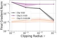
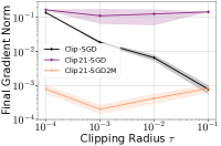
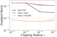
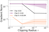
Duke	Leukemia	Duke	Leukemia

Figure 2: Comparison of tuned Clip-SGD, Clip21-SGD, and Clip21-SGD2M on logistic regression with non-convex regularization for various clipping radii $\tau$ with mini-batch (two left) and Gaussian-added (two right) stochastic gradients. The final gradient norm is averaged over the last $100$ iterations. The gradient norm dynamics are reported in Figure˜6.

First, we test the convergence of Clip-SGD, Clip21-SGD, and the proposed Clip21-SGD2M algorithms with stochastic gradients for various clipping radii $\tau$ on several workloads. These results demonstrate the significance of using the momentum technique to achieve better performance.

Non-convex Logistic Regression.

We demonstrate the performance of all algorithms without adding noise for privacy but with stochastic gradients. We consider two cases: adding Gaussian noise to full local gradient $\nabla f_{i}(x)$ and mini-batch stochastic gradient. We conduct experiments on logistic regression with non-convex regularization, namely, $f_{i}(x)=\frac{1}{m}\sum_{j=1}^{m}\log(1+\exp(-b_{ij}a_{ij}^{\top}x))+\lambda\sum_{l=1}^{d}\frac{x_{l}^{2}}{1+x_{l}^{2}}$ which is a typical problem considered in previous works (Khirirat et al., 2023; Li and Chi, 2023). We use the Duke and Leukemia (Chang and Lin, 2011) datasets.

We tune the stepsize $\gamma$ for all algorithms, and momentum parameter $\beta$ for Clip21-SGD2M. Moreover, we set $\hat{\beta}=1$ since we do not add DP noise in this set of experiments. The detailed tuning details are provided in Section˜H.1. We plot the gradient norm averaged across the last $100$ iterations and $3$ different runs in Figure˜2. The results demonstrate the resilience of Clip21-SGD2M to the choice of the clipping radius $\tau$: it achieves a smaller or similar gradient norm compared to two other algorithms over all values of $\tau.$ This is especially visible when the clipping radius $\tau$ is small. These experimental findings align with the theoretical results presented in this work. Besides, the convergence plots are presented in Figure˜6. The results demonstrate that Clip21-SGD2M converges faster than competitors.

Training Resnet20 and VGG16.

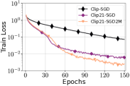
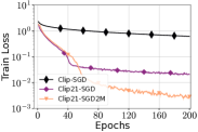
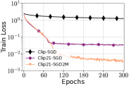
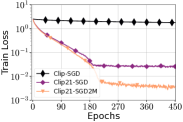
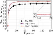
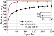
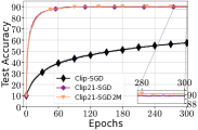
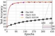
$\tau=10^{-1}$	$\tau=10^{-2}$	$\tau=10^{-3}$	$\tau=10^{-4}$

Figure 7: Comparison of Clip-SGD, Clip21-SGD, and Clip21-SGD2M ($\hat{\beta}=1$) on training VGG16 model on CIFAR10 dataset where the clipping is applied globally.

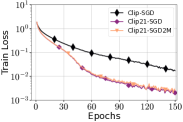
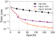
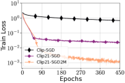
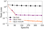
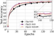
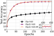
$\tau=10^{-1}$	$\tau=10^{-2}$	$\tau=10^{-3}$	$\tau=10^{-4}$

Figure 8: Comparison of Clip-SGD, Clip21-SGD, and Clip21-SGD2M ($\hat{\beta}=1$) on training VGG16 model on CIFAR10 dataset the clipping is applied layer-wise.

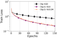
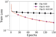
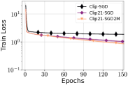
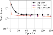
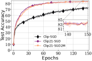
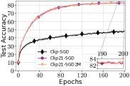
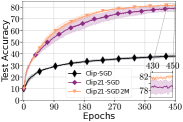
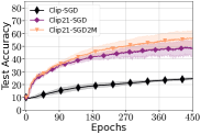
$\tau=10^{-1}$	$\tau=10^{-2}$	$\tau=10^{-3}$	$\tau=10^{-4}$

Figure 9: Comparison of Clip-SGD, Clip21-SGD, and Clip21-SGD2M ($\hat{\beta}=1$) on training Resnet20 model on CIFAR10 dataset where the clipping is applied globally.

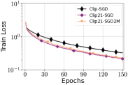
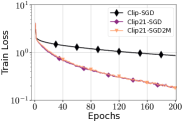
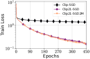
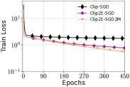
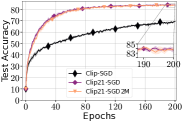
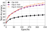
$\tau=10^{-1}$	$\tau=10^{-2}$	$\tau=10^{-3}$	$\tau=10^{-4}$

Figure 10: Comparison of Clip-SGD, Clip21-SGD, and Clip21-SGD2M ($\hat{\beta}=1$) on training Resnet20 model on CIFAR10 dataset where the clipping is applied layer-wise.

Next, we conduct experiments in training Resnet20 (He et al., 2016) and VGG16 (Simonyan and Zisserman, 2014) models on CIFAR10 dataset (Krizhevsky et al., 2009). The results are averaged across $3$ different random seeds and shown in Figure˜3 (the clipping operator is applied on all weights simultaneously) and Figure˜4 (the clipping operator is applied layer-wise). Similar to the previous section, we tune the stepsize $\gamma$ for all algorithms and the momentum parameter $\beta$ for Clip21-SGD2M while setting $\hat{\beta}=1.$ The tuning details are deferred to Section˜H.2.1. We plot the test accuracy and train loss at the last point of the training. The results show that the performance of Clip-SGD consistently deteriorates as the clipping radius $\tau$ decreases, while Clip21-SGD and Clip21-SGD2M are more stable to the changes of $\tau.$ Moreover, Clip21-SGD2M outperforms Clip21-SGD for small values of $\tau$ reaching smaller train loss and larger test accuracy that supports the theoretical claims of this paper. We report the training loss and test accuracy dynamics during the training in Figures 7-8 for VGG and in Figures 9-10 for Resnet20.

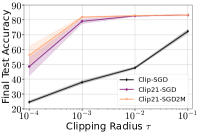
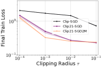
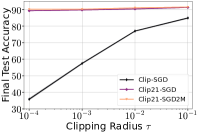
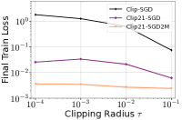
Resnet20, CIFAR10		VGG16, CIFAR10

Figure 3: Comparison of tuned Clip-SGD, Clip21-SGD, and Clip21-SGD2M on training Resnet20 (two left) and VGG16 (two right) models on CIFAR10 dataset where the clipping is applied globally. The train loss and test accuracy dynamics are reported in Figure˜7 and Figure˜9.

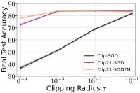
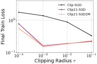
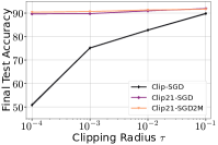
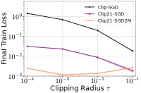
Resnet20, CIFAR10		VGG16, CIFAR10

Figure 4: Comparison of tuned Clip-SGD, Clip21-SGD, and Clip21-SGD2M on training Resnet20 (two left) and VGG16 (two right) models on CIFAR10 dataset where the clipping is applied layer-wise. The training loss and test accuracy dynamics are presented in Figure˜8 and Figure˜10.

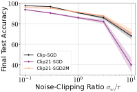
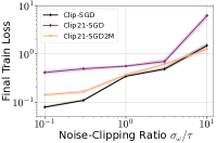
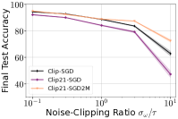
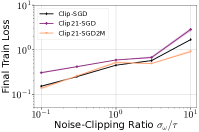
CNN, MNIST		MLP, MNIST

Figure 5: Comparison of tuned Clip-SGD, Clip21-SGD, and Clip21-SGD2M on training CNN (two left) and MLP (two right) models on MNIST dataset varying the noise-clipping ration where the clipping is applied globally. The training loss and test accuracy dynamics are presented in Figure˜12, 11, 14, and 13.

Adding Gaussian Noise for DP.

In the second set of experiments, we test the performance of algorithms with additive Gaussian noise to preserve privacy. Since DP noise variance $\sigma_{\omega}$ typically scales with the clipping radius $\tau$ (e.g., see Corollary˜1), we conduct the following set of experiments: we fix a noise-clipping ratio from $\{0.1,0.3,1.0,3.0,10.0\}$ for neural networks, and find such $\tau$ that gives the lowest train loss or test accuracy depending on the considered workload. The high values of the noise-clipping ratio correspond to stronger DP guarantees, while low values stand for weaker DP guarantees. For each algorithm we tune the stepsize $\gamma$, and additionally the momentum parameters $\beta$ and $\hat{\beta}$ for Clip21-SGD2M (see Section˜H.2.2).

We conduct experiments on training CNN and MLP models on MNIST dataset (Deng, 2012) varying the noise-clipping ratio. We highlight that it is a standard experiment setting considered in the literature on differential privacy (Papernot et al., 2020; Li and Chi, 2023; Allouah et al., 2024). The performance results are reported in Figure˜5. We observe that no algorithm outperforms others across all values of the noise-clipping ratio in terms of the train loss. However, Clip-SGD typically attains smaller train loss than Clip21-SGD2M for a large value of the noise-clipping ratio while Clip21-SGD2M achieves smaller train loss than Clip-SGD when that ratio is small.

5 Conclusion and Future Work

In this work, we introduced a new method called Clip21-SGD2M and proved that it achieves an optimal convergence rate and near optimal privacy-utility trade-off without assuming boundedness of the gradients or boundedness of the data heterogeneity. Notably, several interesting directions remain unexplored. The first one is related to the generalization of the derived results to the case when stochastic gradients have heavy-tailed noise. Next, it would be interesting to study AdaGrad/Adam-type (Streeter and McMahan, 2010; Duchi et al., 2011; Kingma and Ba, 2014) versions of Clip21-SGD2M due to their practical superiority over SGD in solving Deep Learning problems. Finally, it is important to extend the current analysis of Clip21-SGD2M to the case when generalized smoothness is satisfied (Zhang et al., 2020b).

Appendix A Notation

For brevity, in all proofs, we use the following notation

$$\delta^{t}\coloneqq f(x^{t})-f^{*},\quad\widetilde{V}^{t}\coloneqq\frac{1}{n}\sum_{i=1}^{n}\|g_{i}^{t}-v_{i}^{t}\|^{2},$$

$$\widetilde{P}^{t}\coloneqq\frac{1}{n}\sum_{i=1}^{n}\|v_{i}^{t}-\nabla f_{i}(x^{t})\|^{2},\quad P^{t}\coloneqq\|v^{t}-\nabla f(x^{t})\|^{2},$$

$$R^{t}\coloneqq\|x^{t+1}-x^{t}\|^{2}.$$

We additionally denote $\eta^{t}_{i}\coloneqq\frac{\tau}{\|v_{i}^{t}-g_{i}^{t-1}\|}$ and $\eta\coloneqq\frac{\tau}{B}$ where $B$ is defined in each section (it is different in deterministic and stochastic settings). Besides, we define $\mathcal{I}_{t}\coloneqq\{i\in[n]\mid\|v_{i}^{t}-g_{i}^{t-1}\|>\tau\}.$

We denote $\theta_{i}^{t}\coloneqq\nabla f_{i}(x^{t},\xi^{t}_{i})-\nabla f_{i}(x^{t}).$ From ˜2, we have that $\theta_{i}^{t}$ is zero-centered $\sigma$-sub-Gaussian random vector conditioned at $x^{t},$ namely

$$\mathbb{E}\left[\theta^{t}_{i}\mid x^{t}\right]=0,\quad\mathbb{E}\left[\exp\left(\frac{\|\theta^{t}_{i}\|^{2}}{\sigma^{2}}\right)\mid x^{t}\right]\leq\exp(1),$$ (14)

which is equivalent to

$$\Pr(\|\theta^{t}_{i}\|>b)\leq 2\exp\left(-\frac{b^{2}}{2\sigma^{2}}\right)\quad\forall b>0$$ (15)

up to the numerical factor in $\sigma$ [Vershynin, 2018]. Moreover, we define an average of $\theta^{t}_{i}$ as $\theta^{t}\coloneqq\frac{1}{n}\sum_{i=1}^{n}\theta^{t}_{i},$ an average of $\omega^{t}_{i}$ as $\Omega^{t}=\frac{1}{n}\sum_{l=1}^{t}\sum_{i=1}^{n}\omega_{i}^{l},$ and an average of $g_{i}^{t}$ as $\overline{g}^{t}=\frac{1}{n}\sum_{i=1}^{n}g_{i}^{t}$. Thus, we have the following relation between $g^{t}$ and $\overline{g}^{t}:$

$$g^{t}=\overline{g}^{t}+\hat{\beta}\Omega^{t}.$$ (16)

Indeed, it is true at iteration $0$ by the initialization. Let us assume that it holds at iteration $t$, then we have

$$g^{t+1}=g^{t}+\frac{\hat{\beta}}{n}\sum_{i=1}^{n}(\operatorname{clip}_{\tau}(v_{i}^{t+1}-g_{i}^{t})+\omega_{i}^{t+1})=\overline{g}^{t}+\hat{\beta}\Omega^{t}+\frac{\hat{\beta}}{n}\sum_{i=1}^{n}(\operatorname{clip}_{\tau}(v_{i}^{t+1}-g_{i}^{t})+\omega_{i}^{t+1})=\overline{g}^{t+1}+\hat{\beta}\Omega^{t+1},$$

i.e., it holds at iteration $t+1$ as well.

Appendix B Useful Lemmas

Lemma 1 (Lemma C.3 in [Gorbunov et al., 2019]).

Let $\{\xi_{k}\}_{k=1}^{N}$ be the sequence of random vectors with values in $\mathbb{R}^{n}$ such that

$$\mathbb{E}\left[\xi_{k}\mid\xi_{k-1},\dots,\xi_{1}\right]=0\text{ almost surely, }\forall k\in\{1,\dots,N\},$$

and set $S_{N}\coloneqq\sum_{k=1}^{N}\xi_{k}$. Assume that the sequence $\{\xi_{k}\}_{k=1}^{N}$ are sub-Gaussian, i.e.

$$\mathbb{E}\left[\exp\left(\nicefrac{{\|\xi_{k}\|^{2}}}{{\sigma_{k}^{2}}}\mid\xi_{k-1},\dots,\xi_{1}\right)\right]\leq\exp(1)\text{ almost surely, }\forall k\in\{1,\dots,N\},$$

where $\sigma_{2},\dots,\sigma_{N}$ are some positive numbers. Then for all $\gamma\geq 0$

$$\Pr\left(\|S_{N}\|\geq(\sqrt{2}+2\gamma)\sqrt{\sum_{k=1}^{N}\sigma_{k}^{2}}\right)\leq\exp(-\nicefrac{{\gamma^{2}}}{{3}}).$$ (17)

Lemma 2.

Let $f$ be $L$-smooth, $\delta^{t}=f(x^{t})-f^{*}$, $\{x^{t}\}$ be generated by Algorithm˜3, and the stepsize $\gamma\leq\frac{1}{2L}$. Then

$$\begin{aligned} \delta^{t+1}&\leq\delta^{t}-\frac{\gamma}{2}\|\nabla f(x^{t})\|^{2}-\frac{1}{4\gamma}\|x^{t}-x^{t+1}\|^{2}+2\gamma\|\nabla f(x^{t})-v^{t}\|^{2}\\ &\qquad+\;\frac{2\gamma}{n}\sum_{i=1}^{n}\|g_{i}^{t}-v^{t}_{i}\|^{2}+\gamma\hat{\beta}^{2}\|\Omega^{t}\|^{2}.\end{aligned}$$ (18)

Proof.

Using $L$-smoothness of $f$ we have

$$f(x^{t+1}) \overset{(i)}{\leq}f(x^{t})+\langle\nabla f(x^{t}),x^{t+1}-x^{t}\rangle+\frac{L}{2}\|x^{t+1}-x^{t}\|^{2}$$

$$\overset{(ii)}{=}f(x^{t})-\gamma\langle\nabla f(x^{t}),g^{t}\rangle+\frac{L\gamma^{2}}{2}\|g^{t}\|^{2}$$

$$\overset{(iii)}{=}f(x^{t})-\frac{\gamma}{2}\left(\|\nabla f(x^{t})\|^{2}+\|g^{t}\|^{2}-\|\nabla f(x^{t})-g^{t}\|^{2}\right)+\frac{L\gamma^{2}}{2}\|g^{t}\|^{2}$$

$$=f(x^{t})-\frac{\gamma}{2}\|\nabla f(x^{t})\|^{2}-\frac{\gamma}{2}\|g^{t}\|^{2}(1-L\gamma)+\frac{\gamma}{2}\|\nabla f(x^{t})-g^{t}\|^{2}$$

$$\overset{(iv)}{\leq}f(x^{t})-\frac{\gamma}{2}\|\nabla f(x^{t})\|^{2}-\frac{\gamma}{4}\|g^{t}\|^{2}+\frac{\gamma}{2}\|\nabla f(x^{t})-g^{t}\|^{2}.$$ (19)

where $(i)$ follows from smoothness; $(ii)$ from the update rule; $(iii)$ from $\|a-b\|^{2}=\|a\|^{2}+\|b\|^{2}-2\langle a,b\rangle$; $(iv)$ from the stepsize restriction $\gamma\leq\frac{1}{2L}$. Using (16) we continue as follows

$$f(x^{t+1}) \leq f(x^{t})-\frac{\gamma}{2}\|\nabla f(x^{t})\|^{2}-\frac{\gamma}{4}\|g^{t}\|^{2}+\gamma\|\nabla f(x^{t})-\overline{g}^{t}\|^{2}+\gamma\hat{\beta}^{2}\|\Omega^{t}\|^{2}$$

$$\overset{(i)}{\leq}f(x^{t})-\frac{\gamma}{2}\|\nabla f(x^{t})\|^{2}-\frac{\gamma}{4}\|g^{t}\|^{2}+2\gamma\|\nabla f(x^{t})-v^{t}\|^{2}+2\gamma\|\overline{g}^{t}-v^{t}\|^{2}+\gamma\hat{\beta}^{2}\|\Omega^{t}\|^{2}$$

$$\overset{(ii)}{\leq}f(x^{t})-\frac{\gamma}{2}\|\nabla f(x^{t})\|^{2}-\frac{\gamma}{4}\|g^{t}\|^{2}+2\gamma\|\nabla f(x^{t})-v^{t}\|^{2}+\frac{2\gamma}{n}\sum_{i=1}^{n}\|g_{i}^{t}-v^{t}_{i}\|^{2}+\gamma\hat{\beta}^{2}\|\Omega^{t}\|^{2},$$ (20)

where steps $(i$-$ii)$ follow from Young’s inequality. It remains to subtract $f^{*}$ from both sides and replace $g^{t}$ with $\frac{1}{\gamma}(x^{t}-x^{t+1})$.

∎

Lemma 3 (Lemma 4.1 in [Khirirat et al., 2023]).

The clipping operator satisfies for any $x\in\mathbb{R}^{d}$

$$\|\operatorname{clip}_{\tau}(x)-x\|\leq\max\left\{\|x\|-\tau,0\right\}.$$ (21)

Lemma 4 (Property of smooth functions).

Let $\phi\colon\mathbb{R}^{d}\to\mathbb{R}$ be $L$-smooth and lower bounded by $\phi^{*}\in\mathbb{R},$ i.e. $\phi(x)\geq\phi^{*}$ for any $x\in\mathbb{R}^{d}.$ Then we have

$$\|\nabla\phi(x)\|^{2}\leq 2L(\phi(x)-\phi^{*}).$$ (22)

Proof.

It is a standard property of smooth functions. We refer to Theorem 4.23 of [Orabona, 2019]. ∎

Appendix C Proof of Theorem˜1

Proof.

The case $n=1$. Let us consider the problem $f(x)=\frac{L}{2}\|x\|^{2}$. Let vectors $\{z_{j}\}_{j=1}^{3}$ be defined as

$$z_{1}=\begin{pmatrix}3\\ 0\end{pmatrix}\sqrt{\frac{3\sigma^{2}}{100}},\quad z_{2}=\begin{pmatrix}0\\ 4\end{pmatrix}\sqrt{\frac{3\sigma^{2}}{100}},\quad z_{1}=\begin{pmatrix}-3\\ -4\end{pmatrix}\sqrt{\frac{3\sigma^{2}}{100}}.$$

Note that we have

$$\|z_{1}\|^{2}=\frac{27\sigma^{2}}{100},\quad\|z_{2}\|^{2}=\frac{24\sigma^{2}}{50},\quad\|z_{3}\|^{2}=\frac{3\sigma^{2}}{4},$$

meaning that $\tau<\|z_{i}\|$ for all $i\in[3]$. We define the stochastic gradient as $\nabla f(x^{t},\xi^{t})=\nabla f(x^{t})+\xi^{t}=Lx^{t}+\xi^{t}$ where $\xi^{t}$ is picked uniformly at random from $\{z_{1},z_{2},z_{3}\}$. Simple calculations verify that Assumption 2 holds for such noise. Next, the update rule of the method (6) in the case $n=1$ is

$$x^{t+1}=x^{t}-\gamma g^{t}=x^{t}-\gamma(\nabla f(x^{t})+\operatorname{clip}_{\tau}(\nabla f(x^{t},\xi^{t})-\nabla f(x^{t})))=x^{t}-L\gamma x^{t}-\gamma\operatorname{clip}_{\tau}(\xi^{t}).$$

Since $\tau<\|z_{i}\|$ for any $i\in\{1,2,3\}$ clipping is always active and we have

$$\mathbb{E}\left[\operatorname{clip}_{\tau}(\xi^{t})\right] =\frac{1}{3}\operatorname{clip}_{\tau}(z_{1})+\frac{1}{3}\operatorname{clip}_{\tau}(z_{2})+\frac{1}{3}\operatorname{clip}_{\tau}(z_{3})$$

$$=\frac{1}{3}\frac{\tau}{\|z_{1}\|}z_{1}+\frac{1}{3}\frac{\tau}{\|z_{2}\|}z_{2}+\frac{1}{3}\frac{\tau}{\|z_{3}\|}z_{3}$$

$$=\frac{1}{3}\frac{\tau}{\frac{3\sqrt{3}\sigma}{10}}\frac{\sigma\sqrt{3}}{10}\begin{pmatrix}3\\ 0\end{pmatrix}+\frac{1}{3}\frac{\tau}{\frac{4\sqrt{3}\sigma}{10}}\frac{\sigma\sqrt{3}}{10}\begin{pmatrix}0\\ 4\end{pmatrix}+\frac{1}{3}\frac{\tau}{\frac{5\sqrt{3}\sigma}{10}}\frac{\sigma\sqrt{3}}{10}\begin{pmatrix}-3\\ -4\end{pmatrix}$$

$$=\frac{\tau}{9}\begin{pmatrix}3\\ 0\end{pmatrix}+\frac{\tau}{12}\begin{pmatrix}0\\ 4\end{pmatrix}+\frac{\tau}{15}\begin{pmatrix}-3\\ -4\end{pmatrix}$$

$$=\underbrace{\frac{\tau}{15}\begin{pmatrix}2\\ 1\end{pmatrix}}_{\coloneqq h}.$$

Thus, we obtain

$$\mathbb{E}\left[x^{T}\right] =(1-L\gamma)\mathbb{E}\left[x^{T-1}\right]-\gamma\mathbb{E}\left[\operatorname{clip}_{\tau}(\xi^{t})\right]$$

$$=(1-L\gamma)\mathbb{E}\left[x^{T-1}\right]-\gamma h$$

$$=(1-L\gamma)^{T}x^{0}-\gamma h\sum_{t=0}^{T-1}(1-L\gamma)^{T-1-t}$$

$$=(1-L\gamma)^{T}\begin{pmatrix}0\\ x_{(2)}^{0}\end{pmatrix}-\frac{\tau\gamma}{15}\begin{pmatrix}2\\ 1\end{pmatrix}\frac{1-(1-L\gamma)^{T}}{1-(1-L\gamma)}$$

$$=(1-L\gamma)^{T}\begin{pmatrix}0\\ x_{(2)}^{0}\end{pmatrix}-\frac{\tau}{15L}\begin{pmatrix}2\\ 1\end{pmatrix}(1-(1-L\gamma)^{T}).$$

Therefore, since $x_{(2)}^{0}<0$ we have

$$\mathbb{E}\left[\|\nabla f(x^{T})\|^{2}\right] =\mathbb{E}\left[\|Lx^{T}\|^{2}\right]$$

$$=\left\|\mathbb{E}\left[Lx^{T}\right]\right\|^{2}+\mathbb{E}\left[\left\|Lx^{T}-\mathbb{E}\left[Lx^{T}\right]\right\|^{2}\right]$$

$$\geq\left\|\mathbb{E}\left[Lx^{T}\right]\right\|^{2}$$

$$=\frac{4\tau^{2}}{165}\left(1-\left(1-L\gamma\right)^{T}\right)^{2}+L^{2}\left((1-L\gamma)^{T}x^{0}_{(2)}-\frac{\tau}{15L}\left(1-\left(1-L\gamma\right)^{T}\right)\right)^{2}$$

$$\geq\frac{4\tau^{2}}{165}\left(1-\left(1-L\gamma\right)^{T}\right)^{2}+(1-L\gamma)^{2T}\|Lx^{0}\|^{2}+\frac{\tau^{2}}{165}(1-(1-L\gamma)^{T})^{2}$$

$$=\frac{\tau^{2}}{45}\left(1-\left(1-L\gamma\right)^{T}\right)^{2}+(1-L\gamma)^{2T}\|\nabla f(x^{0})\|^{2}.$$

Note that the function $a(1-x)^{2}+x^{2}b\geq\frac{ab}{a+b}.$ Applying this result for $a=\frac{\tau^{2}}{45},b=\|\nabla f(x^{0})\|^{2},$ and $x=(1-L\gamma)^{T}$ we get

$$\mathbb{E}\left[\|\nabla f(x^{T})\|^{2}\right]\geq\frac{\frac{\tau^{2}}{45}\|\nabla f(x^{0})\|^{2}}{\frac{\tau^{2}}{45}+\|\nabla f(x^{0})\|^{2}}\geq\frac{1}{2}\min\left\{\|\nabla f(x^{0})\|^{2},\frac{\tau^{2}}{45}\right\}.$$

The case $n>1$. If $n>1$ then we can consider a similar example where each client is quadratic $\frac{L}{2}\|x\|^{2}$ and the stochastic gradient is constructed as $\nabla f_{i}(x^{t},\xi^{t}_{i})=\nabla f_{i}(x^{t})+\xi^{t}_{i}=Lx^{t}+\xi^{t}_{i}$ where $\xi^{t}_{i}$ is sampled uniformly at random from vectors $\{z_{1},z_{2},z_{3}\}$ such that

$$z_{1}=\begin{pmatrix}3\\ 0\end{pmatrix}\sqrt{\frac{3\sigma^{2}}{100B}},\quad z_{2}=\begin{pmatrix}0\\ 4\end{pmatrix}\sqrt{\frac{3\sigma^{2}}{100B}},\quad z_{1}=\begin{pmatrix}-3\\ -4\end{pmatrix}\sqrt{\frac{3\sigma^{2}}{100B}}.$$

Then, Assumption 2 is satisfied with $\nicefrac{{\sigma^{2}}}{{B}}$. Therefore, if $x_{(2)}^{0}=-1$, $\varepsilon<\frac{L}{\sqrt{2}},$ and $\tau\geq\frac{\varepsilon}{3\sqrt{10}}$, this implies that $B\leq\frac{243\sigma^{2}}{5\varepsilon^{2}}<\frac{27\sigma^{2}}{50\tau^{2}}$, and

$$\mathbb{E}\left[\|\nabla f(x^{T})\|^{2}\right]\geq\frac{1}{2}\min\left\{\|\nabla f(x^{0})\|^{2},\frac{\tau^{2}}{45}\right\}\geq\varepsilon^{2}.$$

∎

Appendix D Proof of Theorem˜2

As we mention in the main part of the paper, the proofs are induction-based: by induction, we show that several quantities remain bounded throughout the work of the method. That is, in Lemmas 5-11, we establish several useful bounds and recurrences. These lemmas allow us to use the contraction-like property (8) of the clipping operator and finish the proof of Theorem 2 applying similar techniques used in the analysis of EF21.

Lemma 5.

Let each $f_{i}$ be $L$-smooth. Then, the iterates generated by Clip21-SGD2M with
$\nabla f_{i}(x^{t+1},\xi^{t+1}_{i})=\nabla f_{i}(x^{t+1})$ (full gradients) and $\sigma_{\omega}=0$ (no DP-noise) satisfy the following inequality

$$\begin{aligned} \|v_{i}^{t+1}-g_{i}^{t}\|&\leq(1-\hat{\beta})\|v_{i}^{t}-g_{i}^{t-1}\|+\hat{\beta}\max\{0,\|v_{i}^{t}-g_{i}^{t-1}\|-\tau\}+L\gamma\beta\|g^{t}\|\\ &\qquad+\beta\|\nabla f_{i}(x^{t})-v_{i}^{t}\|.\end{aligned}$$ (23)

Proof.

We have

$$\|v_{i}^{t+1}-g_{i}^{t}\| \overset{(i)}{=}\|(1-\beta)v_{i}^{t}+\beta\nabla f_{i}(x^{t+1})-g_{i}^{t}\|$$

$$\overset{(ii)}{\leq}\|v_{i}^{t}-g_{i}^{t}\|+\beta\|\nabla f_{i}(x^{t+1})-v_{i}^{t}\|$$

$$\overset{(iii)}{=}\|v_{i}^{t}-g_{i}^{t-1}-\hat{\beta}\operatorname{clip}_{\tau}(v_{i}^{t}-g_{i}^{t-1})\|+\beta\|\nabla f_{i}(x^{t+1})-\nabla f_{i}(x^{t})\|+\beta\|\nabla f_{i}(x^{t})-v_{i}^{t}\|$$

$$\overset{(iv)}{\leq}(1-\hat{\beta})\|v_{i}^{t}-g_{i}^{t-1}\|+\hat{\beta}\|v_{i}^{t}-g_{i}^{t-1}-\operatorname{clip}_{\tau}(v_{i}^{t}-g_{i}^{t-1})\|+L\gamma\beta\|g^{t}\|+\beta\|\nabla f_{i}(x^{t})-v_{i}^{t}\|$$

$$\overset{(v)}{\leq}(1-\hat{\beta})\|v_{i}^{t}-g_{i}^{t-1}\|+\hat{\beta}\max\{0,\|v_{i}^{t}-g_{i}^{t-1}\|-\tau\}+L\gamma\beta\|g^{t}\|+\beta\|\nabla f_{i}(x^{t})-v_{i}^{t}\|.$$

where $(i)$ follows from the update rule of $v_{i}^{t}$ in deterministic case, $(ii)$ from triangle inequality, $(iii)$ from the update rule of $g_{i}^{t}$, $(iv)$ from triangle inequality, update rule of $x^{t}$, and $L$-smoothness, $(v)$ properties of clipping from Lemma˜3. ∎

Lemma 6.

Let each $f_{i}$ be $L$-smooth, $\Delta\geq\Phi^{0}$, and $B>\tau$. Assume that the following inequalities hold for the iterates generated by Clip21-SGD2M with $\nabla f_{i}(x^{t+1},\xi^{t+1}_{i})=\nabla f_{i}(x^{t+1})$ (full gradients) and $\sigma_{\omega}=0$ (no DP-noise)

1. $\|g^{t-1}\|\leq\sqrt{64L\Delta}+3(B-\tau)$;

2. $\|\nabla f_{i}(x^{t-1})-v_{i}^{t-1}\|\leq\sqrt{4L\Delta}+\frac{3}{2}(B-\tau);$

3. $\|v_{i}^{t}-g_{i}^{t-1}\|\leq B$ $\forall i\in[n]$;

4. $\gamma\leq\frac{1}{12L};$

5. $\hat{\beta},\beta\in[0,1];$

6. $\Phi^{t}\leq\Delta$.

Then we have

$$\|g^{t}\|\leq\sqrt{64L\Delta}+3(B-\tau).$$ (24)

Proof.

We have

$$\|g^{t}\|$$

$$\overset{(i)}{=} \left\|g^{t-1}+\frac{\hat{\beta}}{n}\sum_{i=1}^{n}\operatorname{clip}_{\tau}(v_{i}^{t}-g_{i}^{t-1})\right\|$$

$$= \left\|g^{t-1}+\hat{\beta}(v^{t}-g^{t-1})+\frac{\hat{\beta}}{n}\sum_{i=1}^{n}\left(\operatorname{clip}_{\tau}(v_{i}^{t}-g_{i}^{t-1})-(v_{i}^{t}-g_{i}^{t-1})\right)\right\|$$

$$= \left\|(1-\hat{\beta})g^{t-1}+\hat{\beta}\nabla f(x^{t})+\hat{\beta}(v^{t}-\nabla f(x^{t}))+\frac{\hat{\beta}}{n}\sum_{i=1}^{n}\left(\operatorname{clip}_{\tau}(v_{i}^{t}-g_{i}^{t-1})-(v_{i}^{t}-g_{i}^{t-1})\right)\right\|$$

$$\overset{(ii)}{\leq} (1-\hat{\beta})\|g^{t-1}\|+\hat{\beta}\|\nabla f(x^{t})\|+\frac{\hat{\beta}}{n}\sum_{i=1}^{n}\|v_{i}^{t}-\nabla f_{i}(x^{t})\|+\frac{\hat{\beta}}{n}\sum_{i=1}^{n}\max\left\{0,\|v_{i}^{t}-g_{i}^{t-1}\|-\tau\right\},$$

where $(i)$ follows from the update rule $g_{i}^{t}$, $(ii)$ from triangle inequality and clipping properties from Lemma˜3. We continue the derivation of the bound for $\|g^{t}\|$ as follows

$$\|g^{t}\| \overset{(i)}{\leq}(1-\hat{\beta})\|g^{t-1}\|+\hat{\beta}\|\nabla f(x^{t-1})\|+\hat{\beta}\|\nabla f(x^{t})-\nabla f(x^{t-1})\|$$

$$\;+\;\frac{\hat{\beta}}{n}\sum_{i=1}^{n}\|(1-\beta)v_{i}^{t-1}+\beta\nabla f_{i}(x^{t})-\nabla f_{i}(x^{t})\|+\hat{\beta}(B-\tau)$$

$$\overset{(ii)}{\leq}(1-\hat{\beta})\|g^{t-1}\|+\hat{\beta}\sqrt{2L(f(x^{t})-f^{*})}+L\gamma\hat{\beta}\|g^{t-1}\|+\frac{\hat{\beta}}{n}(1-\beta)\sum_{i=1}^{n}\|\nabla f_{i}(x^{t})-v_{i}^{t-1}\|$$

$$\;+\;\hat{\beta}(B-\tau)$$

$$\overset{(iii)}{\leq}(1-\hat{\beta}+L\gamma\hat{\beta})\|g^{t-1}\|+\hat{\beta}\sqrt{2L\Phi^{t}}+\frac{\hat{\beta}}{n}(1-\beta)\sum_{i=1}^{n}\|\nabla f_{i}(x^{t})-\nabla f_{i}(x^{t-1})\|$$

$$\;+\;\frac{\hat{\beta}}{n}(1-\beta)\sum_{i=1}^{n}\|\nabla f_{i}(x^{t-1})-v_{i}^{t-1}\|+\hat{\beta}(B-\tau)$$

$$\overset{(iv)}{\leq}(1-\hat{\beta}+L\gamma\hat{\beta}(2-\beta))\|g^{t-1}\|+\hat{\beta}\sqrt{2L\Delta}+\hat{\beta}(1-\beta)(\sqrt{4L\Delta}+\frac{3}{2}(B-\tau))+\hat{\beta}(B-\tau)$$

$$\overset{(v)}{\leq}(1-\hat{\beta}+L\gamma\hat{\beta}(2-\beta))(\sqrt{64L\Delta}+3(B-\tau))+\hat{\beta}\sqrt{2L\Delta}+\hat{\beta}(1-\beta)(\sqrt{4L\Delta}+\frac{3}{2}(B-\tau))$$

$$\;+\;\hat{\beta}(B-\tau),$$

where $(i)$ follows from triangle inequality and update of $v_{i}^{t}$, $(ii)$ from $L$-smoothness and update rule of $x^{t}$, $(iii)$ from the definition of $\Phi^{t}$ and triangle inequality, $(iv)$ from the assumptions $2$ and $6$, $(v)$ from the assumption $1$. The above is satisfied if we have simultaneously

$$8(1-\hat{\beta}+2L\gamma\hat{\beta})+\sqrt{2}\hat{\beta}+2\hat{\beta} \leq 8$$

$$3(1-\hat{\beta}+2L\gamma\hat{\beta})+\frac{3}{2}\hat{\beta}+\hat{\beta} \leq 3.$$

Both inequalities hold when $L\gamma\leq\frac{1}{12}.$ ∎

Lemma 7.

Let each $f_{i}$ be $L$-smooth, $\Delta\geq\Phi^{0}$, and $B>\tau$. Assume that the following inequalities hold for the iterates generated by Clip21-SGD2M with $\nabla f_{i}(x^{t+1},\xi^{t+1}_{i})=\nabla f_{i}(x^{t+1})$ (full gradients) and $\sigma_{\omega}=0$ (no DP-noise)

1. $4L\gamma\leq\beta$ and $\gamma\leq\frac{1}{4L};$

2. $\|\nabla f_{i}(x^{t-1})-v_{i}^{t-1}\|\leq\sqrt{4L\Delta}+\frac{3}{2}(B-\tau)$;

3. $\|g^{t-1}\|\leq\sqrt{64L\Delta}+3(B-\tau).$

Then we have

$$\|\nabla f_{i}(x^{t})-v_{i}^{t}\|\leq\sqrt{4L\Delta}+\frac{3}{2}(B-\tau)\quad\forall i\in[n].$$ (25)

Proof.

We have

$$\|\nabla f_{i}(x^{t})-v_{i}^{t}\| \overset{(i)}{=}\|\nabla f_{i}(x^{t})-(1-\beta)v_{i}^{t-1}-\beta\nabla f_{i}(x^{t})\|$$

$$=(1-\beta)\|\nabla f_{i}(x^{t})-v_{i}^{t-1}\|$$

$$\overset{(ii)}{\leq}(1-\beta)L\gamma\|g^{t-1}\|+(1-\beta)\|\nabla f_{i}(x^{t-1})-v_{i}^{t-1}\|$$

$$\overset{(iii)}{\leq}L\gamma\left(\sqrt{64L\Delta}+3(B-\tau)\right)+(1-\beta)\left(\sqrt{4L\Delta}+\frac{3}{2}(B-\tau)\right)$$

$$=(8L\gamma+2(1-\beta))\sqrt{L\Delta}+\left(3L\gamma+\frac{3(1-\beta)}{2}\right)(B-\tau),$$

where $(i)$ follows from the update rule of $v_{i}^{t}$, $(ii)$ from triangle inequality, smoothness, and update of $x^{t}$, $(iii)$ from conditions $2$-$3$ in the statement of the lemma. We need to satisfy

$$8L\gamma+2(1-\beta)\leq 2\Leftrightarrow 4L\gamma\leq\beta.$$

$$3L\gamma+\frac{3}{2}(1-\beta)\leq\frac{3}{2}\Leftrightarrow 2L\gamma\leq\beta.$$

Since $4L\gamma\leq\beta$, both inequalities are satisfied. ∎

Lemma 8.

Let each $f_{i}$ be $L$-smooth, $\Delta\geq\Phi^{0}$, $B>\tau$, and $i\in\mathcal{I}_{t}\coloneqq\{i\in[n]\mid\|v_{i}^{t}-g_{i}^{t-1}\|>\tau\}$. Assume that the following inequalities hold for the iterates generated by Clip21-SGD2M with $\nabla f_{i}(x^{t+1},\xi^{t+1}_{i})=\nabla f_{i}(x^{t+1})$ (full gradients) and $\sigma_{\omega}=0$ (no DP-noise)

1. $4L\gamma\leq\beta$;

2. $L\gamma\leq\frac{1}{12};$

3. $\frac{8}{3}\beta\sqrt{L\Delta}\leq\frac{\hat{\beta}\tau}{4};$

4. $\frac{7}{4}\beta(B-\tau)\leq\frac{\hat{\beta}\tau}{4}$;

5. $\|g^{t}\|\leq\sqrt{64L\Delta}+3(B-\tau);$

6. $\|\nabla f_{i}(x^{t})-v_{i}^{t}\|\leq\sqrt{4L\Delta}+\frac{3}{2}(B-\tau).$

Then

$$\|v_{i}^{t+1}-g_{i}^{t}\|\leq\|v_{i}^{t}-g_{i}^{t-1}\|-\frac{\hat{\beta}\tau}{2}.$$ (26)

Proof.

Since $i\in\mathcal{I}_{t}$, then $\|v_{i}^{t}-g_{i}^{t-1}\|>\tau$, thus from Lemma˜5 we have

$$\|v_{i}^{t+1}-g_{i}^{t}\| \leq(1-\hat{\beta})\|v_{i}^{t}-g_{i}^{t-1}\|+\hat{\beta}(\|v_{i}^{t}-g_{i}^{t-1}\|-\tau)+\beta L\gamma\|g^{t}\|+\beta\|\nabla f_{i}(x^{t})-v_{i}^{t}\|$$

$$\overset{(i)}{\leq}\|v_{i}^{t}-g_{i}^{t-1}\|-\hat{\beta}\tau+\beta L\gamma\left(\sqrt{64L\Delta}+3(B-\tau)\right)+\beta\left(\sqrt{4L\Delta}+\frac{3}{2}(B-\tau)\right)$$

$$=\|v_{i}^{t}-g_{i}^{t-1}\|-\hat{\beta}\tau+(8\beta L\gamma+2\beta)\sqrt{L\Delta}+(3\beta L\gamma+\nicefrac{{3\beta}}{{2}})(B-\tau),$$

where $(i)$ follows from assumptions $5$-$6$ of the statement of the lemma. Since $L\gamma\leq\frac{1}{12},$ we have

$$\|v_{i}^{t+1}-g_{i}^{t}\| \leq\|v_{i}^{t}-g_{i}^{t-1}\|-\hat{\beta}\tau+\frac{8}{3}\beta\sqrt{L\Delta}+\frac{7}{4}\beta(B-\tau).$$

Due to assumptions $2$-$3$ of the lemma, we have

$$\|v_{i}^{t+1}-g_{i}^{t}\| \leq\|v_{i}^{t}-g_{i}^{t-1}\|-\frac{\hat{\beta}\tau}{2},$$

which concludes the proof. ∎

Lemma 9.

Let each $f_{i}$ be $L$-smooth. Then, for the iterates generated by Clip21-SGD2M with $\nabla f_{i}(x^{t+1},\xi^{t+1}_{i})=\nabla f_{i}(x^{t+1})$ (full gradients) and $\sigma_{\omega}=0$ (no DP-noise) the quantity
$\widetilde{P}^{t}\coloneqq\frac{1}{n}\sum_{i=1}^{n}\|v_{i}^{t}-\nabla f_{i}(x^{t})\|^{2}$ decreases as

$$\widetilde{P}^{t+1}\leq(1-\beta)\widetilde{P}^{t}+\frac{3L^{2}}{\beta}R^{t}.$$ (27)

Proof.

We have

$$\|v_{i}^{t+1}-\nabla f_{i}(x^{t+1})\|^{2} \overset{(i)}{=}\|(1-\beta)v_{i}^{t}+\beta\nabla f_{i}(x^{t+1})-\nabla f_{i}(x^{t+1})\|^{2}$$

$$=(1-\beta)^{2}\|\nabla f_{i}(x^{t+1})-v_{i}^{t}\|^{2}$$

$$\overset{(ii)}{\leq}(1-\beta)^{2}(1+\nicefrac{{\beta}}{{2}})\|v_{i}^{t}-\nabla f_{i}(x^{t})\|^{2}$$

$$\qquad+(1-\beta)^{2}(1+\nicefrac{{2}}{{\beta}})\|\nabla f_{i}(x^{t})-\nabla f_{i}(x^{t+1})\|^{2}$$

$$\overset{(iii)}{\leq}(1-\beta)\|v_{i}^{t}-\nabla f_{i}(x^{t})\|^{2}+\frac{3L^{2}}{\beta}\|x^{t}-x^{t+1}\|^{2},$$

where $(i)$ follows from the update rule of $v_{i}^{t}$, $(ii)$ – from the inequality $\|a+b\|^{2}\leq(1+\beta/2)\|a\|^{2}+(1+2/\beta)\|b\|^{2}$ that holds for any $a,b\in\mathbb{R}^{d}$ and $\beta>0$, and $(iii)$ – from $(1-\beta)(1+\nicefrac{{\beta}}{{2}})\leq 1$, which holds for any $\beta\in[0,1]$, and smoothness. Averaging the inequalities above across $i\in[n],$ we get the statement of the lemma. ∎

Similarly, we can get the recursion for $P^{t}\coloneqq\|v^{t}-\nabla f(x^{t})\|^{2}$.

Lemma 10.

Let each $f_{i}$ be $L$-smooth. Then, for the iterates generated by Clip21-SGD2M with $\nabla f_{i}(x^{t+1},\xi^{t+1}_{i})=\nabla f_{i}(x^{t+1})$ (full gradients) and $\sigma_{\omega}=0$ (no DP-noise) the quantity
$P^{t}\coloneqq\|v^{t}-\nabla f(x^{t})\|^{2}$ decreases as

$$P^{t+1}\leq(1-\beta)P^{t}+\frac{3L^{2}}{\beta}R^{t}.$$ (28)

Next, we establish the recursion for $\widetilde{V}^{t}\coloneqq\frac{1}{n}\sum_{i=1}^{n}\|g_{i}^{t}-v_{i}^{t}\|^{2}$.

Lemma 11.

Let each $f_{i}$ be $L$-smooth. Consider Clip21-SGD2M with $\nabla f_{i}(x^{t+1},\xi^{t+1}_{i})=\nabla f_{i}(x^{t+1})$ (full gradients) and $\sigma_{\omega}=0$ (no DP-noise). Let $\|v_{i}^{t}-g_{i}^{t-1}\|\leq B$, for all $i\in[n]$ and some $B\geq\tau$, and $\hat{\beta}\leq\frac{1}{2\eta}$ . Then

$$\|g_{i}^{t}-v_{i}^{t}\|^{2}\leq(1-\hat{\beta}\eta)\|g_{i}^{t-1}-v_{i}^{t-1}\|^{2}+\frac{4\beta^{2}}{\hat{\beta}\eta}\|v_{i}^{t-1}-\nabla f_{i}(x^{t-1})\|^{2}+\frac{4L^{2}\beta^{2}}{\hat{\beta}}R^{t-1}.$$

and, in particular,

$$\widetilde{V}^{t}\leq(1-\eta)\widetilde{V}^{t-1}+\frac{4\beta^{2}}{\hat{\beta}\eta}\widetilde{P}^{t-1}+\frac{4\beta^{2}L^{2}}{\hat{\beta}\eta}R^{t-1},$$

where $\eta\coloneqq\frac{\tau}{B}$, $R^{t}\coloneqq\|x^{t+1}-x^{t}\|^{2}$, and $\widetilde{V}^{t}\coloneqq\frac{1}{n}\sum\limits_{i=1}^{n}\|g_{i}^{t}-v_{i}^{t}\|^{2}$.

Proof.

Since $\|v_{i}^{t}-g_{i}^{t-1}\|\leq B$, for $\eta^{t}_{i}\coloneqq\frac{\tau}{\|v_{i}^{t}-g_{i}^{t-1}\|}$ we have $\eta^{t}_{i}\geq\eta$. This implies

$$\|g_{i}^{t}-v_{i}^{t}\|^{2} \overset{(i)}{=}\|g_{i}^{t-1}+\hat{\beta}\operatorname{clip}_{\tau}(v_{i}^{t}-g_{i}^{t-1})-v_{i}^{t}\|^{2}$$

$$=\|\hat{\beta}(g_{i}^{t-1}-v_{i}^{t}+\operatorname{clip}_{\tau}(v_{i}^{t}-g_{i}^{t-1}))+(1-\hat{\beta})(g_{i}^{t-1}-v_{i}^{t})\|^{2}$$

$$\overset{(ii)}{\leq}(1-\eta)^{2}\hat{\beta}\|g_{i}^{t-1}-v_{i}^{t}\|^{2}+(1-\hat{\beta})\|g_{i}^{t-1}-v_{i}^{t}\|^{2},$$

where $(i)$ follows from the update rule of $g_{i}^{t}$ and $(ii)$ from the convexity of $\|\cdot\|^{2}$ and the fact that $\|v_{i}^{t}-g_{i}^{t-1}\|\leq B.$ We continue the derivations as follows

$$\|g_{i}^{t}-v_{i}^{t}\|^{2} =(1-\hat{\beta}+\hat{\beta}(1-2\eta+\eta^{2}))\|g_{i}^{t-1}-v_{i}^{t}\|^{2}$$

$$=(1-\hat{\beta}\eta(2-\eta))\|g_{i}^{t-1}-v_{i}^{t}\|^{2}.$$

Let $\rho=2\hat{\beta}\eta$ (note that $\eta\leq 1$). Then we have

$$\|g_{i}^{t}-v_{i}^{t}\|^{2} \leq(1-\rho)\|g_{i}^{t-1}-v_{i}^{t}\|^{2}$$

$$\overset{(i)}{=}(1-\rho)\|g_{i}^{t-1}-(1-\beta)v_{i}^{t-1}-\beta\nabla f_{i}(x^{t})\|^{2}$$

$$\overset{(ii)}{\leq}(1-\rho)(1+\nicefrac{{\rho}}{{2}})\|g_{i}^{t-1}-v_{i}^{t-1}\|^{2}+(1-\rho)(1+\nicefrac{{2}}{{\rho}})\beta^{2}\|v_{i}^{t-1}-\nabla f_{i}(x^{t})\|^{2}$$

$$\overset{(iii)}{\leq}(1-\nicefrac{{\rho}}{{2}})\|g_{i}^{t-1}-v_{i}^{t-1}\|^{2}+\frac{4\beta^{2}}{\rho}\|v_{i}^{t-1}-\nabla f_{i}(x^{t-1})\|^{2}+\frac{4L^{2}\beta^{2}}{\rho}R^{t-1},$$

where $(i)$ follows from the update rule of $g_{i}^{t}$, $(ii)$ from the inequality $\|a+b\|^{2}\leq(1+r/2)\|a\|^{2}+(1+2/r)\|b\|^{2}$, which holds for any positive $r$ (i.e., for $r=\rho$ for some $\rho>0$) and $a,b\in\mathbb{R}^{d}$, $(iii)$ from the fact that $\rho\leq 1$ by assumption, the inequality $\|a+b\|^{2}\leq 2\|a\|^{2}+2\|b\|^{2}$, which holds for any $a,b\in\mathbb{R}^{d}$, and smoothness. Finally, since $2\hat{\beta}\eta\leq 1,$ we ensure that $\rho\leq 1,$ and derive the final bound

$$\|g_{i}^{t}-v_{i}^{t}\|^{2} \leq(1-\hat{\beta}\eta)\|g_{i}^{t-1}-v_{i}^{t-1}\|^{2}+\frac{4\beta^{2}}{\hat{\beta}\eta}\|v_{i}^{t-1}-\nabla f_{i}(x^{t-1})\|^{2}+\frac{4L^{2}\beta^{2}}{\hat{\beta}}R^{t-1}.$$

∎

Theorem 5 (Full statement of Theorem˜2).

Let Assumption 1 hold. Let
$B\coloneqq\max\{3\tau,\max_{i}\|\nabla f_{i}(x^{0})\|\}$ and $\Phi^{0}$ defined in (10) satisfies $\Delta\geq\Phi^{0}$ for some $\Delta>0$. Assume the following inequalities hold

1. stepsize restrictions: $\gamma\leq\frac{1}{12L},4L\gamma=\beta$, and

   $$\frac{5}{8}-\frac{32\beta^{2}L^{2}}{\hat{\beta}^{2}\eta^{2}}\gamma^{2}-\frac{96L^{2}}{\hat{\beta}^{2}\eta^{2}}\gamma^{2}\geq 0;$$

2. momentum restrictions: $\frac{8}{3}\beta\sqrt{L\Delta}\leq\frac{\hat{\beta}\tau}{4},\frac{7}{4}\beta(B-\tau)\leq\frac{\hat{\beta}\tau}{4},\hat{\beta}\leq\frac{1}{2\eta}$.

Then, the Lyapunov function from (10) for Clip21-SGD2M with $\nabla f_{i}(x^{t+1},\xi^{t+1}_{i})=\nabla f_{i}(x^{t+1})$ (full gradients) and $\sigma_{\omega}=0$ (no DP-noise) decreases as

$$\Phi^{t+1}\leq\Phi^{t}-\frac{\gamma}{2}\|\nabla f(x^{t})\|^{2},$$

and we have

$$\frac{1}{T}\sum_{t=0}^{T-1}\|\nabla f(x^{t})\|^{2}\leq\frac{2\Delta}{\gamma T}=\mathcal{O}\left(\frac{1}{T}\right).$$ (29)

Moreover, after at most $\frac{2B}{\hat{\beta}\tau}$ iterations, the clipping operator will be turned off for all workers.

Proof.

For convenience, we define

$$\nabla f_{i}(x^{-1})=v_{i}^{-1}=g_{i}^{-1}=0,\quad\Phi^{-1}=+\infty.$$

Then, we will derive the result by induction, i.e., using the induction w.r.t. $t$, we will show that

1. the Lyapunov function decreases as $\Phi^{t}\leq\Phi^{t-1}-\frac{\gamma}{2}\|\nabla f(x^{t-1})\|^{2};$

2. $\|g^{t}\|\leq\sqrt{64L\Delta}+3(B-\tau)$;

3. $\|v_{i}^{t}-\nabla f_{i}(x^{t})\|\leq\sqrt{4L\Delta}+\frac{3}{2}(B-\tau);$

4. $\|v_{i}^{t}-g_{i}^{t-1}\|\leq\max\left\{0,B-\frac{t\hat{\beta}\tau}{2}\right\}.$

First, we prove that the base of induction holds.

Base of induction.

1. $\|v_{i}^{0}-g_{i}^{-1}\|=\|v_{i}^{0}\|=\beta\|\nabla f_{i}(x^{0})\|\leq\frac{1}{2}B\leq B$ holds;

2. $g^{0}=\frac{1}{n}\sum_{i=1}^{n}(g_{i}^{-1}+\hat{\beta}\operatorname{clip}_{\tau}(v_{i}^{0}-g_{i}^{-1})=\frac{\hat{\beta}}{n}\sum_{i=1}^{n}\operatorname{clip}_{\tau}(\beta\nabla f_{i}(x^{0})).$ Therefore, we have

   $$\|g^{0}\| \leq\left\|\frac{\hat{\beta}}{n}\sum_{i=1}^{n}\beta\nabla f_{i}(x^{0})+(\operatorname{clip}_{\tau}(\beta\nabla f_{i}(x^{0}))-\beta\nabla f_{i}(x^{0}))\right\|$$

   $$\leq\hat{\beta}\beta\|\nabla f(x^{0})\|+\frac{\hat{\beta}}{n}\sum_{i=1}^{n}\max\left\{0,\beta\|\nabla f_{i}(x^{0})\|-\tau\right\}$$

   $$\leq\hat{\beta}\beta\sqrt{2L(f(x^{0})-f^{*})}+\hat{\beta}(B-\tau)$$

   $$\leq\sqrt{64L\Delta}+3(B-\tau).$$

3. We have

   $$\|v_{i}^{0}-\nabla f_{i}(x^{0})\| =\|\beta\nabla f_{i}(x^{0})-\nabla f_{i}(x^{0})\|$$

   $$\leq(1-\beta)B$$

   $$\leq\sqrt{4L\Delta}+\frac{3}{2}(B-\tau)$$

4. $\Phi^{0}\leq\Phi^{-1}-\frac{\gamma}{2}\|\nabla f(x^{-1})\|^{2}=\Phi^{-1}$ holds.

Transition of induction.

Assume that for $K$ we have that for all $t\in\{0,1,\ldots,K\}$

1. $\Phi^{t}\leq\Phi^{t-1}-\frac{\gamma}{2}\|\nabla f(x^{t-1})\|^{2}$ (implying $\Phi^{t}\leq\Delta$);

2. $\|g^{t}\|\leq\sqrt{64L\Delta}+3(B-\tau);$

3. $\|v_{i}^{t}-\nabla f_{i}(x^{t})\|\leq\sqrt{4L\Delta}+\frac{3}{2}(B-\tau);$

4. $\|v_{i}^{t}-g_{i}^{t-1}\|\leq\max\left\{\hat{\beta}\tau,B-\frac{t\hat{\beta}\tau}{2}\right\}.$

We proceed via analyzing two possible situations for $\mathcal{I}_{K+1}\coloneqq\{i\in[n]\mid\|v_{i}^{K+1}-g_{i}^{K}\|>\tau\}$: either $|\mathcal{I}_{K+1}|>0$ (there are workers with turned on gradient clipping) or $|\mathcal{I}_{K+1}|=0$ (for all workers the clipping is turned off).

Case $|\mathcal{I}_{K+1}|>0.$

Since all requirements of Lemma˜8 are satisfied at iteration $K$ we get for all $i\in\mathcal{I}_{K+1}$

$$\|v_{i}^{K+1}-g_{i}^{K}\|\leq\|v_{i}^{K}-g_{i}^{K-1}\|-\frac{\hat{\beta}\tau}{2}\overset{(i)}{\leq}\max\left\{\tau,B-\frac{K\hat{\beta}\tau}{2}\right\}-\frac{\hat{\beta}\tau}{2}\leq\max\left\{\tau,B-\frac{(K+1)\hat{\beta}\tau}{2}\right\},$$

where (i) follows from the condition 4 of the induction assumption. Similarly due to the assumption of induction, from Lemma˜6 we get that

$$\|g^{K+1}\|\leq\sqrt{64L\Delta}+3(B-\tau),$$

and from Lemma˜7

$$\|\nabla f_{i}(x^{K+1})-v_{i}^{K+1}\|\leq\sqrt{4L\Delta}+\frac{3}{2}(B-\tau).$$

This means that conditions $2$-$4$ in the assumption of the induction are also verified for step $K+1$. The remaining part is the descent of the Lyapunov function. For estimating
$\widetilde{V}^{K+1}\coloneqq\frac{1}{n}\sum\limits_{i=1}^{n}\|g_{i}^{K+1}-v_{i}^{K+1}\|^{2}$ we have Lemma˜11 since $\|v_{i}^{K+1}-g_{i}^{K}\|\leq B-\frac{\tau}{2}$

$$\widetilde{V}^{K+1}\leq(1-\hat{\beta}\eta)\widetilde{V}^{K}+\frac{4\beta^{2}}{\hat{\beta}\eta}\widetilde{P}^{K}+\frac{4\beta^{2}L^{2}}{\hat{\beta}\eta}R^{K}.$$

Combining this result with the claims of Lemmas˜2, 9 and 10 we get

$$\Phi^{K+1} =\delta^{K+1}+\frac{2\gamma}{\hat{\beta}\eta}\widetilde{V}^{K+1}+\frac{8\gamma\beta}{\hat{\beta}^{2}\eta^{2}}\widetilde{P}^{K+1}+\frac{2\gamma}{\beta}P^{K+1}$$

$$\leq\delta^{K}-\frac{\gamma}{2}\|\nabla f(x^{K})\|^{2}-\frac{1}{4\gamma}R^{K}+2\gamma\widetilde{V}^{K}+2\gamma P^{K}$$

$$\;+\;\frac{2\gamma}{\hat{\beta}\eta}\left((1-\hat{\beta}\eta)\widetilde{V}^{K}+\frac{4\beta^{2}}{\hat{\beta}\eta}\widetilde{P}^{K}+\frac{4\beta^{2}L^{2}}{\hat{\beta}\eta}R^{K}\right)$$

$$\;+\;\frac{8\gamma\beta}{\hat{\beta}^{2}\eta^{2}}\left((1-\beta)\widetilde{P}^{K}+\frac{3L^{2}}{\beta}R^{K}\right)$$

$$\;+\;\frac{2\gamma}{\beta}\left((1-\beta)P^{K}+\frac{3L^{2}}{\beta}R^{K}\right)$$

$$=\delta^{K}-\frac{\gamma}{2}\|\nabla f(x^{K})\|^{2}+\frac{2\gamma}{\hat{\beta}\eta}\widetilde{V}^{K}\left(1-\hat{\beta}\eta+\hat{\beta}\eta\right)+\frac{8\gamma\beta}{\hat{\beta}^{2}\eta^{2}}\widetilde{P}^{K}\left(1-\beta+\beta\right)$$

$$\;+\;\frac{2\gamma}{\beta}P^{K}\left(1-\beta+\beta\right)-\frac{1}{4\gamma}\left(1-\frac{32\beta^{2}L^{2}}{\hat{\beta}^{2}\eta^{2}}\gamma^{2}-\frac{96L^{2}}{\hat{\beta}^{2}\eta^{2}}\gamma^{2}-\frac{24L^{2}}{\beta^{2}}\gamma^{2}\right)R^{K}$$

$$=\Phi^{K}-\frac{\gamma}{2}\|\nabla f(x^{K})\|^{2}-\frac{1}{4\gamma}\left(1-\frac{32\beta^{2}L^{2}}{\hat{\beta}^{2}\eta^{2}}\gamma^{2}-\frac{96L^{2}}{\hat{\beta}^{2}\eta^{2}}\gamma^{2}-\frac{24L^{2}}{\beta^{2}}\gamma^{2}\right)R^{K}.$$

Since we choose $\beta^{2}=64L^{2}\gamma^{2},$ then $-\frac{1}{\beta^{2}}=-\frac{1}{64L^{2}\gamma^{2}}$ and $-\frac{24L^{2}}{\beta^{2}}\gamma^{2}=-\frac{24L^{2}}{64^{2}L^{2}\gamma^{2}}\gamma^{2}\geq-\frac{3}{8}$ Therefore,

$$1-\frac{32\beta^{2}L^{2}}{\eta^{2}}\gamma^{2}-\frac{96L^{2}}{\hat{\beta}^{2}\eta^{2}}\gamma^{2}-\frac{24L^{2}}{\beta^{2}}\gamma^{2} \geq\frac{5}{8}-\frac{32\beta^{2}L^{2}}{\hat{\beta}^{2}\eta^{2}}\gamma^{2}-\frac{96L^{2}}{\hat{\beta}^{2}\eta^{2}}\gamma^{2}\geq 0,$$

by the choice of $\gamma.$ Thus, we get

$$\Phi^{K+1}\leq\Phi^{K}-\frac{\gamma}{2}\|\nabla f(x^{K})\|^{2}.$$

In particular, this implies $\Phi^{K+1}\leq\Phi^{K}\leq\Delta.$

Case $|\mathcal{I}_{K+1}|=0$.

In this case, $\eta^{K+1}_{i}=1$ for all $i\in[n]$, i.e., $\operatorname{clip}_{\tau}(v_{i}^{K+1}-g_{i}^{K})=v_{i}^{K+1}-g_{i}^{K}$ that leads to $g_{i}^{K+1}=v_{i}^{K+1}$. Thus, $\widetilde{V}^{K+1}=0$. Moreover, $|\mathcal{I}_{K+1}|=0$ implies that condition 4 from the induction assumption holds for $t=K+1$ and using this and induction assumption we get $\|g^{K+1}\|\leq\sqrt{64L\Delta}+3(B-\tau)$ from Lemma˜6 and $\|\nabla f_{i}(x^{K+1})-v_{i}^{K+1}\|\leq\sqrt{4L\Delta}+\frac{3}{2}(B-\tau)$ from Lemma˜7. Next, taking into account that $\widetilde{V}^{K+1}=0$, we can perform similar steps as before for $\Phi^{K+1}$ and get less restrictive inequality

$$\Phi^{K+1} \leq\Phi^{K}-\frac{\gamma}{2}\|\nabla f(x^{K})\|^{2}-\frac{1}{4\gamma}\left(1-\frac{96L^{2}}{\hat{\beta}^{2}\eta^{2}}\gamma^{2}-\frac{24L^{2}}{\beta^{2}}\gamma^{2}\right)R^{K}.$$

Again, $1-\frac{96L^{2}}{\hat{\beta}^{2}\eta^{2}}\gamma^{2}-\frac{24L^{2}}{\beta^{2}}\gamma^{2}\geq\frac{5}{8}-\frac{96L^{2}}{\hat{\beta}^{2}\eta^{2}}\gamma^{2}\geq 0$ which is satisfied by the choice of $\gamma.$

We conclude that in both cases the Lyapunov function decreases as $\Phi^{K+1}\leq\Phi^{K}-\frac{\gamma}{2}\|\nabla f(x^{K})\|^{2}$, and consequently, $\Phi^{K+1}\leq\Delta.$ This finalizes the induction step. Therefore, we can guarantee that for all iterations $t\in\{0,1,\ldots,T-1\}$ we have

$$\Phi^{t+1}\leq\Phi^{t}-\frac{\gamma}{2}\|\nabla f(x^{t})\|^{2}\Rightarrow\frac{1}{T}\sum_{t=0}^{T-1}\|\nabla f(x^{t})\|^{2}\leq\frac{2\Delta}{\gamma T}.$$

Moreover, the proof shows that the clipping operator will be eventually turned off after at most $\frac{2B}{\hat{\beta}\tau}$ iterations since $\|v_{i}^{t}-g_{i}^{t-1}\|\leq\max\left\{\tau,B-\frac{t\hat{\beta}\tau}{2}\right\}$. ∎

Appendix E Proof of Theorem˜4

The proof of Theorem˜4 is split into two parts: small and large DP noise.

We define constants $a$, $b$, and $c$, which will be used later in the proofs, as follows:

$$a \coloneqq\left(\sqrt{2}+2\sqrt{3\log\frac{6(T+1)}{\alpha}}\right)\sqrt{d}\sigma_{\omega}\sqrt{\frac{T}{n}},$$

$$b^{2} \coloneqq 2\sigma^{2}\log\left(\frac{12(T+1)n}{\alpha}\right),$$ (30)

$$c^{2} \coloneqq\left(\sqrt{2}+2\sqrt{3\log\frac{6(T+1)}{\alpha}}\right)^{2}\sigma^{2},$$

where $T$ is the number of iterations, $n$ is the number of workers, $d$ is the dimension of the problem, $\sigma$ is from ˜2, $\alpha\in(0,1)$ is a constant, and $\sigma_{\omega}$ is the variance of DP noise.

Lemma 12.

Let each $f_{i}$ be $L$-smooth. Then, for the iterates of Clip21-SGD2M we have the following inequality with probability $1$

$$\begin{aligned} \|v_{i}^{t+1}-g_{i}^{t}\|&\leq(1-\hat{\beta})\|v_{i}^{t}-g_{i}^{t-1}\|+\hat{\beta}\max\left\{0,\|v_{i}^{t}-g_{i}^{t-1}\|-\tau\right\}+\beta L\gamma\|g^{t}\|\\ &\qquad+\beta\|\nabla f_{i}(x^{t})-v_{i}^{t}\|+\beta\|\theta^{t+1}_{i}\|,\end{aligned}$$ (31)

where $\theta_{i}^{t}\coloneqq\nabla f_{i}(x^{t},\xi^{t}_{i})-\nabla f_{i}(x^{t})$.

Proof.

We have

$$\|v_{i}^{t+1}-g_{i}^{t}\| \overset{(i)}{=}\|(1-\beta)v_{i}^{t}+\beta\nabla f_{i}(x^{t+1},\xi^{t+1}_{i})-g_{i}^{t}\|$$

$$\overset{(ii)}{\leq}\|v_{i}^{t}-g_{i}^{t}\|+\beta\|\nabla f_{i}(x^{t+1},\xi^{t+1}_{i})-v_{i}^{t}\|$$

$$\overset{(iii)}{=}\|v_{i}^{t}-\hat{\beta}\operatorname{clip}_{\tau}(v_{i}^{t}-g_{i}^{t-1})-g_{i}^{t-1}\|+\beta\|\nabla f_{i}(x^{t+1},\xi^{t+1}_{i})-v_{i}^{t}\|$$

$$\overset{(iv)}{\leq}(1-\hat{\beta})\|v_{i}^{t}-g_{i}^{t-1}\|+\hat{\beta}\max\left\{0,\|v_{i}^{t}-g_{i}^{t-1}\|-\tau\right\}+\beta\|\nabla f_{i}(x^{t+1},\xi_{i}^{t+1})-\nabla f_{i}(x^{t+1})\|$$

$$\quad+\beta\|\nabla f_{i}(x^{t+1})-\nabla f_{i}(x^{t})\|+\beta\|\nabla f_{i}(x^{t})-v_{i}^{t}\|$$

$$\overset{(v)}{\leq}(1-\hat{\beta})\|v_{i}^{t}-g_{i}^{t-1}\|+\hat{\beta}\max\left\{0,\|v_{i}^{t}-g_{i}^{t-1}\|-\tau\right\}+\beta L\|x^{t+1}-x^{t}\|$$

$$\qquad+\beta\|\nabla f_{i}(x^{t})-v_{i}^{t}\|+\beta\|\theta^{t+1}_{i}\|$$

$$\overset{(vi)}{=}(1-\hat{\beta})\|v_{i}^{t}-g_{i}^{t-1}\|+\hat{\beta}\max\left\{0,\|v_{i}^{t}-g_{i}^{t-1}\|-\tau\right\}+\beta L\gamma\|g^{t}\|$$

$$\qquad+\beta\|\nabla f_{i}(x^{t})-v_{i}^{t}\|+\beta\|\theta^{t+1}_{i}\|,$$

where $(i)$ follows from the update rule of $v_{i}^{t}$, $(ii)$ from triangle inequality, $(iii)$ from the update rule of $g_{i}^{t}$, $(iv)$ from the properties of the clipping operator from Lemma˜3 and triangle inequality, $(v)$ from smoothness, $(vi)$ from the update rule of $x^{t}.$ ∎

Lemma 13.

Let each $f_{i}$ be $L$-smooth, $\Delta\geq\Phi^{0}$. Assume that the following inequalities hold for the iterates generated by Clip21-SGD2M

1. $g^{0}=\frac{1}{n}\sum_{i=1}^{n}g_{i}^{0};$

2. $\|g^{t-1}\|\leq\sqrt{64L\Delta}+3(B-\tau)+3b+3\hat{\beta}a$;

3. $\|\overline{g}^{t-1}\|\leq\sqrt{64L\Delta}+3(B-\tau)+3b;$

4. $\|\nabla f_{i}(x^{t-1})-v_{i}^{t-1}\|\leq\sqrt{4L\Delta}+\frac{3}{2}(B-\tau)+\frac{3}{2}b+\hat{\beta}a$ for all $i\in[n];$

5. $\|v_{i}^{t}-g_{i}^{t-1}\|\leq B$ for all $i\in[n];$

6. $\gamma\leq\frac{1}{12L};$

7. $\|\theta^{t}_{i}\|\leq b$ for all $i\in[n];$

8. $\left\|\frac{1}{n}\sum_{l=1}^{t}\sum_{i=1}^{n}\omega_{i}^{l}\right\|\leq a$;

9. $\beta,\hat{\beta}\in[0,1];$

10. $\Phi^{t-1}\leq 2\Delta.$

Then we have

$$\|g^{t}\|\leq\sqrt{64L\Delta}+3(B-\tau)+3b+3\hat{\beta}a.$$ (32)

Proof.

We start as follows

$$\|g^{t}\| \overset{(i)}{=}\left\|g^{t-1}+\frac{\hat{\beta}}{n}\sum_{i=1}^{n}\operatorname{clip}_{\tau}(v_{i}^{t}-g_{i}^{t-1})+\frac{\hat{\beta}}{n}\sum_{i=1}^{n}\omega^{t}_{i}\right\|$$

$$=\left\|g^{t-1}+\frac{\hat{\beta}}{n}\sum_{i=1}^{n}\left[\nabla f_{i}(x^{t})+(v_{i}^{t}-\nabla f_{i}(x^{t}))+\operatorname{clip}_{\tau}(v_{i}^{t}-g_{i}^{t-1})-(v_{i}^{t}-g_{i}^{t-1})\right]\right.$$

$$\quad-\left.\overline{g}^{t-1}+(1-\hat{\beta})\overline{g}^{t-1}+\frac{\hat{\beta}}{n}\sum_{i=1}^{n}\omega^{t}_{i}\right\|$$

$$\overset{(ii)}{\leq}\left\|g^{t-1}-\overline{g}^{t-1}+\frac{\hat{\beta}}{n}\sum_{i=1}^{n}\omega_{i}^{t}\right\|+\hat{\beta}\|\nabla f(x^{t})\|+\frac{\hat{\beta}}{n}\sum_{i=1}^{n}\|\operatorname{clip}_{\tau}(v_{i}^{t}-g_{i}^{t-1})-v_{i}^{t}+g_{i}^{t-1}\|$$

$$\quad+(1-\hat{\beta})\|\overline{g}^{t-1}\|+\frac{\hat{\beta}}{n}\sum_{i=1}^{n}\|v_{i}^{t}-\nabla f_{i}(x^{t})\|$$

$$\overset{(iii)}{\leq}\left\|\overline{g}^{t-1}+\hat{\beta}\Omega^{t-1}-\overline{g}^{t-1}+\frac{\hat{\beta}}{n}\sum_{i=1}^{n}\omega_{i}^{t}\right\|+\hat{\beta}\|\nabla f(x^{t-1})\|+\hat{\beta}\|\nabla f(x^{t})-\nabla f(x^{t-1})\|$$

$$\quad+\frac{\hat{\beta}}{n}\sum_{i=1}^{n}\|\operatorname{clip}_{\tau}(v_{i}^{t}-g_{i}^{t-1})-v_{i}^{t}+g_{i}^{t-1}\|+(1-\hat{\beta})\|\overline{g}^{t-1}\|$$

$$\quad+\frac{\hat{\beta}}{n}\sum_{i=1}^{n}\|(1-\beta)v_{i}^{t-1}+\beta\nabla f_{i}(x^{t},\xi^{t}_{i})-\nabla f_{i}(x^{t})\|,$$

where $(i)$ follows from the update rule of $g^{t}$, $(ii)$ – from the triangle inequality, $(iii)$ – from the update rule of $v_{i}^{t}$, equality (16), and triangle inequality. Using the definition of $\Omega^{t}$, we continue as follows

$$\|g^{t}\| \overset{(iv)}{\leq}\hat{\beta}\|\Omega^{t}\|+\hat{\beta}\|\nabla f(x^{t-1})\|+\hat{\beta}L\gamma\|g^{t-1}\|+\frac{\hat{\beta}}{n}\sum_{i=1}^{n}\max\{0,\|v_{i}^{t}-g_{i}^{t-1}\|-\tau\}+(1-\hat{\beta})\|\overline{g}^{t-1}\|$$

$$\quad+\frac{\hat{\beta}}{n}\sum_{i=1}^{n}\|(1-\beta)v_{i}^{t-1}+\beta\nabla f_{i}(x^{t},\xi_{i}^{t})-\nabla f_{i}(x^{t})\|$$

$$\overset{(v)}{\leq}\hat{\beta}\sqrt{2L(f(x^{t-1})-f^{*})}+\hat{\beta}L\gamma\|g^{t-1}\|+(1-\hat{\beta})\|\overline{g}^{t-1}\|+\hat{\beta}(B-\tau)+\hat{\beta}\|\Omega^{t}\|$$

$$\quad+\frac{\hat{\beta}}{n}\sum_{i=1}^{n}\left((1-\beta)\|v_{i}^{t-1}-\nabla f_{i}(x^{t})\|+\beta\|\nabla f_{i}(x^{t},\xi^{t}_{i})-\nabla f_{i}(x^{t})\|\right)$$

$$\overset{(vi)}{\leq}\hat{\beta}\sqrt{2L(f(x^{t-1})-f^{*})}+\hat{\beta}L\gamma\|g^{t-1}\|+(1-\hat{\beta})\|\overline{g}^{t-1}\|+\hat{\beta}(B-\tau)+\hat{\beta}\|\Omega^{t}\|$$

$$\quad+\frac{\hat{\beta}\beta}{n}\sum_{i=1}^{n}\|\theta^{t}_{i}\|+\frac{\hat{\beta}}{n}(1-\beta)\sum_{i=1}^{n}\left(\|v_{i}^{t-1}-\nabla f_{i}(x^{t-1})\|+\|\nabla f_{i}(x^{t})-\nabla f_{i}(x^{t-1})\|\right)$$

$$\overset{(vii)}{\leq}\hat{\beta}\sqrt{2L(f(x^{t-1})-f^{*})}+\hat{\beta}L\gamma(2-\beta)\|g^{t-1}\|+(1-\hat{\beta})\|\overline{g}^{t-1}\|+\hat{\beta}(B-\tau)+\hat{\beta}\|\Omega^{t}\|$$

$$\quad+\frac{\hat{\beta}\beta}{n}\sum_{i=1}^{n}\|\theta^{t}_{i}\|+\frac{\hat{\beta}}{n}(1-\beta)\sum_{i=1}^{n}\|v_{i}^{t-1}-\nabla f_{i}(x^{t-1})\|.$$

$(iv)$ – from the properties of the clipping operator from Lemma˜3, $L$-smoothness and update rule of $x^{t}$, $(v)$ – from $L$-smoothness and triagnle inequality, $(vi)$ – from triangle inequality, $(vii)$ – from $L$-smoothness. Now we use the assumptions $2$-$5$, $7$-$8$, and $10$ to bound the terms

$$\|g^{t}\| \leq\hat{\beta}\sqrt{4L\Delta}+2L\gamma\hat{\beta}\left(\sqrt{64L\Delta}+3(B-\tau)+3b+3\hat{\beta}a\right)+(1-\hat{\beta})\left(\sqrt{64L\Delta}+3(B-\tau)+3b\right)$$

$$\quad+\hat{\beta}(B-\tau)+\hat{\beta}a+\hat{\beta}\beta b+\hat{\beta}(1-\beta)\left(\sqrt{4L\Delta}+\frac{3}{2}(B-\tau)+\frac{3}{2}b+\hat{\beta}a\right).$$

Regrouping the terms we obtain

$$\|g^{t}\| \leq\sqrt{L\Delta}[2\hat{\beta}+16L\gamma\hat{\beta}+8(1-\hat{\beta})+2\hat{\beta}(1-\beta)]+b[6L\gamma\hat{\beta}+3(1-\hat{\beta})+\hat{\beta}\beta+\nicefrac{{3}}{{2}}\hat{\beta}(1-\beta)]$$

$$\quad+(B-\tau)[6L\gamma\hat{\beta}+3(1-\hat{\beta})+\hat{\beta}+\nicefrac{{3}}{{2}}\hat{\beta}(1-\beta)]+a[6L\gamma\hat{\beta}^{2}+\hat{\beta}+\hat{\beta}^{2}(1-\beta)].$$

For the first coefficient, we have

$$2\hat{\beta}+16L\gamma\hat{\beta}+8(1-\hat{\beta})+2\hat{\beta}(1-\beta)\leq 8\Leftarrow 4\hat{\beta}+16L\gamma\hat{\beta}\leq 8\hat{\beta}\Leftarrow 4L\gamma\leq 1,$$

where the last inequality is satisfied by the choice of the stepsize $L\gamma\leq\frac{1}{12}.$ For the second coefficient, we have

$$6L\gamma\hat{\beta}+3(1-\hat{\beta})+\hat{\beta}\beta+\frac{3}{2}\hat{\beta}(1-\beta)\leq 3\Leftarrow 6L\gamma\hat{\beta}+\hat{\beta}\beta+\frac{3}{2}\hat{\beta}(1-\beta)\leq 3\hat{\beta}$$

$$\Leftarrow\; 6L\gamma+1+\frac{3}{2}(1-\beta)\leq 3,$$

where the last inequality is satisfied by the choice of the stepsize $6L\gamma\leq\frac{1}{2}$ and momentum parameter $\beta\leq 1$. For the third coefficient, we have

$$6L\gamma\hat{\beta}+3(1-\hat{\beta})+\hat{\beta}+\frac{3}{2}\hat{\beta}(1-\beta)\leq 3\Leftarrow 6L\gamma\hat{\beta}+\hat{\beta}+\frac{3}{2}\hat{\beta}(1-\beta)\leq 3\hat{\beta}\Leftarrow 6L\gamma+1+\frac{3}{2}\leq 3,$$

where the last inequality is satisfied by the choice of the stepsize $6L\gamma\leq\frac{1}{2}$. For the fourth coefficient, we have

$$6L\gamma\hat{\beta}^{2}+\hat{\beta}+\hat{\beta}^{2}(1-\beta)\leq 3\hat{\beta}\Leftarrow 6L\gamma\hat{\beta}^{2}+\hat{\beta}^{2}\leq 2\hat{\beta}\Leftarrow 6L\gamma\hat{\beta}+\hat{\beta}\leq 2,$$

where the last inequality is satisfied by the choice of the stepsize $6L\gamma\leq\frac{1}{2}$ and momentum parameter $\hat{\beta}\leq 1.$ Thus, the statement of the lemma holds. ∎

Lemma 14.

Let each $f_{i}$ be $L$-smooth, $\Delta\geq\Phi^{0}$, $B>\tau$. Assume that the following inequalities hold for the iterates generated by Clip21-SGD2M

1. $\gamma\leq\frac{1}{12L}$;

2. $6L\gamma\leq\beta$;

3. $\|\nabla f_{i}(x^{t-1})-v_{i}^{t-1}\|\leq\sqrt{4L\Delta}+\frac{3}{2}(B-\tau)+\frac{3}{2}b+\hat{\beta}a$ for all $i\in[n];$

4. $\|\theta^{t}_{i}\|\leq b$ for all $i\in[n];$

5. $\|g^{t-1}\|\leq\sqrt{64L\Delta}+3(B-\tau)+3b+3\hat{\beta}a;$

6. $\|\overline{g}^{t-1}\|\leq\sqrt{64L\Delta}+3(B-\tau)+3b.$

Then we have

$$\|\nabla f_{i}(x^{t})-v_{i}^{t}\|\leq\sqrt{4L\Delta}+\frac{3}{2}(B-\tau)+\frac{3}{2}b+\hat{\beta}a.$$ (33)

Proof.

We have

$$\|\nabla f_{i}(x^{t})-v_{i}^{t}\| \overset{(i)}{=}\|\nabla f_{i}(x^{t})-(1-\beta)v_{i}^{t-1}-\beta\nabla f_{i}(x^{t},\xi^{t}_{i})\|$$

$$\overset{(ii)}{\leq}(1-\beta)\|\nabla f_{i}(x^{t})-v_{i}^{t-1}\|+\beta\|\nabla f_{i}(x^{t})-\nabla f_{i}(x^{t},\xi^{t}_{i})\|$$

$$\overset{(iii)}{\leq}(1-\beta)L\gamma\|g^{t-1}\|+(1-\beta)\|\nabla f_{i}(x^{t-1})-v_{i}^{t-1}\|+\beta\|\theta^{t}_{i}\|$$

$$\overset{(iv)}{\leq}(1-\beta)L\gamma\left(\sqrt{64L\Delta}+3(B-\tau)+3b+3\hat{\beta}a\right)$$

$$\quad+(1-\beta)\left(\sqrt{4L\Delta}+\frac{3}{2}(B-\tau)+\frac{3}{2}b+\hat{\beta}a\right)+\beta b$$

$$=(8L\gamma+2(1-\beta))\sqrt{L\Delta}+(3L\gamma+\nicefrac{{3(1-\beta)}}{{2}})(B-\tau)$$

$$\quad+(3L\gamma(1-\beta)+\nicefrac{{3}}{{2}}(1-\beta)+\beta)b+(3L\gamma\hat{\beta}+(1-\beta)\hat{\beta})a,$$

where $(i)$ follows from the update rule of $v_{i}^{t}$, $(ii)$ from the triangle inequality, $(iii)$ from triangle inequality, smoothness, and the update rule of $x^{t}$, $(iv)$ from assumptions $2$-$4$ of the lemma. We notice that

$$8L\gamma+2(1-\beta)\leq 2\Leftarrow 4L\gamma\leq\beta,$$

$$3L\gamma+\frac{3}{2}(1-\beta)\leq\frac{3}{2}\Leftarrow 2L\gamma\leq\beta,$$

$$3L\gamma+\frac{3}{2}(1-\beta)+\beta\leq\frac{3}{2}\beta\Leftarrow 6L\gamma\leq\beta,$$

$$3L\gamma\hat{\beta}+(1-\beta)\hat{\beta}\leq\hat{\beta}\Leftarrow 3L\gamma\leq\beta,$$

where the last inequalities in each line are satisfied for $\beta$, satisfying the conditions of the lemma. ∎

Lemma 15.

Let each $f_{i}$ be $L$-smooth, $\Delta\geq\Phi^{0},B>\tau.$ Assume that the following inequalities hold for the iterates generated by Clip21-SGD2M

1. $\gamma\leq\frac{1}{12L};$

2. $\hat{\beta}\leq\min\{\frac{\sqrt{L\Delta}}{a},1\}$;

3. $\|v_{i}^{t}-g_{i}^{t-1}\|\leq B$ for all $i\in[n];$

4. $\|g^{t-1}\|\leq\sqrt{64L\Delta}+3(B-\tau)+3b+\hat{\beta}a;$

5. $\|\overline{g}^{t-1}\|\leq\sqrt{64L\Delta}+3(B-\tau)+3b);$

6. $\|\nabla f_{i}(x^{t-1})-v_{i}^{t-1}\|\leq\sqrt{4L\Delta}+\frac{3}{2}(B-\tau)+\frac{3}{2}b+\hat{\beta}a$ for all $i\in[n];$

7. $\Phi^{t-1}\leq 2\Delta;$

8. $\|\theta_{i}^{t}\|\leq b$ for all $i\in[n].$

Then we have

$$\|\overline{g}^{t}\|\leq\sqrt{64L\Delta}+3(B-\tau)+3b.$$

Proof.

We have

$$\|\overline{g}^{t}\| \overset{(i)}{=}\left\|\overline{g}^{t-1}+\frac{\hat{\beta}}{n}\sum_{i=1}^{n}\operatorname{clip}_{\tau}(v_{i}^{t}-g_{i}^{t-1})\right\|$$

$$=\left\|\hat{\beta}\nabla f(x^{t})+\hat{\beta}(v^{t}-\nabla f(x^{t}))+(1-\hat{\beta})\overline{g}^{t-1}+\frac{\hat{\beta}}{n}\sum_{i=1}^{n}[\operatorname{clip}_{\tau}(v_{i}^{t}-g_{i}^{t-1})-(v_{i}^{t}-g_{i}^{t-1})]\right\|$$

$$\overset{(ii)}{\leq}\hat{\beta}\|\nabla f(x^{t})\|+\frac{\hat{\beta}}{n}\sum_{i=1}^{n}\|v_{i}^{t}-\nabla f_{i}(x^{t})\|+(1-\hat{\beta})\|\overline{g}^{t-1}\|$$

$$\quad+\frac{\hat{\beta}}{n}\sum_{i=1}^{n}\|\operatorname{clip}_{\tau}(v_{i}^{t}-g_{i}^{t-1})-(v_{i}^{t}-g_{i}^{t-1})\|$$

$$\overset{(iii)}{\leq}\hat{\beta}\|\nabla f(x^{t-1})\|+\hat{\beta}L\gamma\|g^{t-1}\|+\frac{\hat{\beta}}{n}\sum_{i=1}^{n}\|(1-\beta)v_{i}^{t-1}+\beta\nabla f_{i}(x^{t},\xi^{t}_{i})-\nabla f_{i}(x^{t})\|$$

$$\quad+(1-\hat{\beta})\|\overline{g}^{t-1}\|+\frac{\hat{\beta}}{n}\sum_{i=1}^{n}\max\{0,\|v_{i}^{t}-g_{i}^{t-1}\|-\tau\}$$

$$\overset{(iv)}{\leq}\hat{\beta}\sqrt{2L(f(x^{t-1})-f^{*})}+\hat{\beta}L\gamma\|g^{t-1}\|+(1-\hat{\beta})\|\overline{g}^{t-1}\|+\hat{\beta}(B-\tau)$$

$$\quad+\frac{\hat{\beta}}{n}\sum_{i=1}^{n}\left((1-\beta)[\|v_{i}^{t-1}-\nabla f_{i}(x^{t-1})\|+\|\nabla f_{i}(x^{t-1})-\nabla f_{i}(x^{t})\|]+\beta\|\nabla f_{i}(x^{t})-\nabla f_{i}(x^{t},\xi^{t}_{i})\|\right),$$

where $(i)$ follows from the update rule of each $g_{i}^{t}$, $(ii)$ – from the triangle inequality, $(iii)$ – from the update of $v_{i}^{t}$ and properties of clipping from Lemma˜3, $(iv)$ – from $L$-smoothness, assumption $3$ of the lemma, and triangle inequality. Now we use assumptions $4$-$7$ to derive

$$\|g^{t}\| \leq\hat{\beta}\sqrt{4L\Delta}+\hat{\beta}L\gamma(2-\beta)\left(\sqrt{64L\Delta}+3(B-\tau)+3b+\hat{\beta}a\right)+\hat{\beta}(B-\tau)$$

$$\quad+(1-\hat{\beta})\left(\sqrt{64L\Delta}+3(B-\tau)+3b\right)+\hat{\beta}(1-\beta)\left(\sqrt{4L\Delta}+\frac{3}{2}(B-\tau)+\frac{3}{2}b+\hat{\beta}a\right)+\hat{\beta}\beta b$$

$$=\sqrt{L\Delta}\left(2\hat{\beta}+8L\gamma(2-\beta)\hat{\beta}+8(1-\hat{\beta})+2\hat{\beta}(1-\beta)\right)+a(L\gamma\hat{\beta}^{2}(2-\beta)+\hat{\beta}^{2})$$

$$\quad+(B-\tau)\left(3L\gamma\hat{\beta}(2-\beta)+\hat{\beta}+3(1-\hat{\beta})+\frac{3}{2}\hat{\beta}(1-\beta)\right)$$

$$\quad+b(3L\gamma\hat{\beta}(2-\beta)+3(1-\hat{\beta})+\nicefrac{{3}}{{2}}\hat{\beta}(1-\beta)).$$

For the second term, we have

$$2L\gamma\hat{\beta}^{2}a+\hat{\beta}^{2}a\leq 2L\gamma\hat{\beta}\sqrt{L\Delta}+\hat{\beta}\sqrt{L\Delta}=(2L\gamma\hat{\beta}+\hat{\beta})\sqrt{L\Delta},$$

where we use $\hat{\beta}\leq\frac{\sqrt{L\Delta}}{a}.$ Therefore, the second term should be added to the first term. Thus, we have for the term with $\sqrt{L\Delta}$

$$2L\gamma\hat{\beta}+\hat{\beta}+2\hat{\beta}+8L\gamma\hat{\beta}(2-\beta)+8(1-\hat{\beta})+2\hat{\beta}(1-\beta)\leq 8$$

$$\Leftarrow\; 2L\gamma+1+2+8L\gamma(2-\beta)+2(1-\beta)\leq 8$$

$$\Leftarrow\; 18L\gamma\leq 3,$$

where the last inequality is satisfied by the choice of the stepsize $L\gamma\leq\frac{1}{12}.$ For the third coefficient, we have

$$3L\gamma\hat{\beta}(2-\beta)+\hat{\beta}+3(1-\hat{\beta})+\frac{3}{2}\hat{\beta}(1-\beta)\leq 3\Leftarrow 3L\gamma(2-\beta)+1+\frac{3}{2}(1-\beta)\leq 3\Leftarrow 6L\gamma\leq\frac{1}{2},$$

where the last inequality is satisfied by the choice of the stepsize $L\gamma\leq\frac{1}{12}.$ For the fourth coefficient, we have the same derivations as for the third one. This implies that

$$\|g^{t}\|\leq 8\sqrt{L\Delta}+3(B-\tau)+3b,$$

which concludes the proof.

∎

Lemma 16.

Let each $f_{i}$ be $L$-smooth, $\Delta\geq\Phi^{0}$, $B>\tau$, and $i\in\mathcal{I}_{t}\coloneqq\{i\in[n]\mid\|v_{i}^{t}-g_{i}^{t-1}\|>\tau\}$. Assume that the following inequalities hold for the iterates generated by Clip21-SGD2M

1. $12L\gamma\leq 1;$

2. $6L\gamma\leq\beta;$

3. $\beta\leq\min\{\frac{3\hat{\beta}\tau}{64\sqrt{L\Delta}},1\}$;

4. $\beta\leq\min\{\frac{\hat{\beta}\tau}{14(B-\tau)},1\};$

5. $\beta\leq\min\{\frac{\hat{\beta}\tau}{22b},1\}$;

6. $\hat{\beta}\leq\min\{\frac{\sqrt{L\Delta}}{a},1\};$

7. $\|g^{t}\|\leq\sqrt{64L\Delta}+3(B-\tau)+3b+3a;$

8. $\|\theta^{t+1}_{i}\|\leq b;$

9. $\|\nabla f_{i}(x^{t})-v_{i}^{t}\|\leq\sqrt{4L\Delta}+\frac{3}{2}(B-\tau)+\frac{3}{2}b+\hat{\beta}a.$

Then

$$\|v_{i}^{t+1}-g_{i}^{t}\|\leq\|v_{i}^{t}-g_{i}^{t-1}\|-\frac{\hat{\beta}\tau}{2}.$$ (34)

Proof.

Since $i\in\mathcal{I}_{t}$, then $\|v_{i}^{t}-g_{i}^{t-1}\|>\tau$ and from Lemma˜12 we have

$$\|v_{i}^{t+1}-g_{i}^{t}\| \leq(1-\hat{\beta})\|v_{i}^{t}-g_{i}^{t-1}\|+\hat{\beta}\|v_{i}^{t}-g_{i}^{t-1}\|-\hat{\beta}\tau+\beta L\gamma\|g^{t}\|+\beta\|\nabla f_{i}(x^{t})-v_{i}^{t}\|+\beta\|\theta^{t+1}_{i}\|$$

$$\overset{(i)}{\leq}\|v_{i}^{t}-g_{i}^{t-1}\|-\hat{\beta}\tau+\beta L\gamma\left(\sqrt{64L\Delta}+3(B-\tau)+3b+3\hat{\beta}a\right)$$

$$\;+\;\beta\left(\sqrt{4L\Delta}+\frac{3}{2}(B-\tau)+\frac{3}{2}b+\hat{\beta}a\right)+\beta b$$

$$=\|v_{i}^{t}-g_{i}^{t-1}\|-\hat{\beta}\tau+(8\beta L\gamma+2\beta)\sqrt{L\Delta}+(3L\gamma\beta+\nicefrac{{3\beta}}{{2}})(B-\tau)$$

$$\;+\;(3L\gamma\beta+\nicefrac{{3\beta}}{{2}}+\beta)b+(3L\gamma\beta+\beta)\hat{\beta}a,$$

where $(i)$ follows from assumptions $6$-$8$ of the lemma. Since $12L\gamma\leq 1$ we have

$$(8\beta L\gamma+2\beta)\sqrt{L\Delta}\leq(\nicefrac{{2\beta}}{{3}}+2\beta)\sqrt{L\Delta}=\frac{8}{3}\beta\sqrt{L\Delta}\leq\frac{\hat{\beta}\tau}{8},$$

where we used $\beta\leq\frac{3\hat{\beta}\tau}{64\sqrt{L\Delta}}.$ Since $12L\gamma\leq\beta$ we have

$$\left(3L\gamma\beta+\frac{3\beta}{2}\right)(B-\tau)\leq(\nicefrac{{\beta}}{{4}}+\frac{3\beta}{2})(B-\tau)=\frac{7}{4}\beta(B-\tau)\leq\frac{\hat{\beta}\tau}{8},$$

where we used $\beta\leq\frac{\hat{\beta}\tau}{14(B-\tau)}$. Since $12L\gamma\leq\beta$ we have

$$(3L\gamma\beta+\nicefrac{{5\beta}}{{2}})b\leq\left(\nicefrac{{\beta}}{{4}}+\nicefrac{{5\beta}}{{2}}\right)b=\frac{11}{4}\beta b\leq\frac{\hat{\beta}\tau}{8},$$

where we used $\beta\leq\frac{\hat{\beta}\tau}{22b}.$ Since $12L\gamma\leq\beta$ and $\hat{\beta}\leq\frac{\sqrt{L\Delta}}{a}$ we have

$$\left(3L\gamma\beta+\beta\right)\hat{\beta}a\leq(\nicefrac{{\beta}}{{4}}+\beta)\sqrt{L\Delta}=\frac{5}{4}\beta\sqrt{L\Delta}\leq\frac{\hat{\beta}\tau}{8},$$

where we used $\beta\leq\frac{\hat{\beta}\tau}{22b}.$ Thus we have

$$\|v_{i}^{t+1}-g_{i}^{t}\| \leq\|v_{i}^{t}-g_{i}^{t-1}\|-\hat{\beta}\tau+4\cdot\frac{\hat{\beta}\tau}{8}=\|v_{i}^{t}-g_{i}^{t-1}\|-\frac{\hat{\beta}\tau}{2},$$

which concludes the proof. ∎

Lemma 17.

Let $\|\theta^{t+1}_{i}\|\leq b$ for all $i\in[n]$. Let each $f_{i}$ be $L$-smooth. Then, for the iterates generated by Clip21-SGD2M the quantity $\widetilde{P}^{t}\coloneqq\frac{1}{n}\sum_{i=1}^{n}\|v_{i}^{t}-\nabla f_{i}(x^{t})\|^{2}$ decreases as

$$\widetilde{P}^{t+1}\leq(1-\beta)\widetilde{P}^{t}+\frac{3L^{2}}{\beta}R^{t}+\beta^{2}b^{2}+\frac{2}{n}\beta(1-\beta)\sum_{i=1}^{n}\langle v_{i}^{t}-\nabla f_{i}(x^{t+1}),\theta^{t+1}_{i}\rangle,$$ (35)

where $R^{t}\coloneqq\|x^{t+1}-x^{t}\|$ and $\theta^{t}_{i}\coloneqq\nabla f_{i}(x^{t},\xi^{t}_{i})-\nabla f_{i}(x^{t})$.

Proof.

We have

$$\|v_{i}^{t+1}-\nabla f_{i}(x^{t+1})\|^{2} \overset{(i)}{=}\|(1-\beta)v_{i}^{t}+\beta\nabla f_{i}(x^{t+1},\xi^{t+1}_{i})-\nabla f_{i}(x^{t+1})\|^{2}$$

$$=\|(1-\beta)(v_{i}^{t}-\nabla f_{i}(x^{t+1}))+\beta(\nabla f_{i}(x^{t+1},\xi^{t+1}_{i})-\nabla f_{i}(x^{t+1}))\|^{2}$$

$$=(1-\beta)^{2}\|v_{i}^{t}-\nabla f_{i}(x^{t+1})\|^{2}+\beta^{2}\|\theta^{t+1}_{i}\|^{2}$$

$$\quad+2\beta(1-\beta)\langle v_{i}^{t}-\nabla f_{i}(x^{t+1}),\theta^{t+1}_{i}\rangle$$

$$\overset{(ii)}{\leq}(1-\beta)^{2}(1+\nicefrac{{\beta}}{{2}})\|v_{i}^{t}-\nabla f_{i}(x^{t})\|^{2}$$

$$\quad+(1-\beta)^{2}(1+\nicefrac{{2}}{{\beta}})\|\nabla f_{i}(x^{t})-\nabla f_{i}(x^{t+1})\|^{2}+\beta^{2}b^{2}$$

$$\quad+2\beta(1-\beta)\langle v_{i}^{t}-\nabla f_{i}(x^{t+1}),\theta^{t+1}_{i}\rangle$$

$$\overset{(iii)}{\leq}(1-\beta)\|v_{i}^{t}-\nabla f_{i}(x^{t})\|^{2}+\frac{3L^{2}}{\beta}\|x^{t}-x^{t+1}\|^{2}+\beta^{2}b^{2}$$

$$\quad+2\beta(1-\beta)\langle v_{i}^{t}-\nabla f_{i}(x^{t+1}),\theta^{t+1}_{i}\rangle,$$

where $(i)$ follows from the update rule of $v_{i}^{t}$, $(ii)$ from $\|x+y\|^{2}\leq(1+r)\|x\|^{2}+(1+r^{-1})\|y\|^{2}$ for any $x,y\in\mathbb{R}^{d}$ and $r>0$, $(iii)$ from the smoothness and inequalities $(1-\beta)^{2}(1+\nicefrac{{\beta}}{{2}})\leq(1-\beta)$ and $(1-\beta)^{2}(1+\nicefrac{{2}}{{\beta}})\leq\nicefrac{{3}}{{\beta}}$. Averaging the inequalities above across all $i\in[n]$, we get the lemma’s statement. ∎

Similarly, we can get the recursion for $P^{t}\coloneqq\|v^{t}-\nabla f(x^{t})\|^{2}$.

Lemma 18.

Let $\|\theta^{t+1}\|\leq\frac{c}{\sqrt{n}}$ for all $i\in[n]$. Let each $f_{i}$ be $L$-smooth. Then, for the iterates generated by Clip21-SGD2M the quantity $P^{t}\coloneqq\|v^{t}-\nabla f(x^{t})\|^{2}$ decreases as

$$P^{t+1}\leq(1-\beta)P^{t}+\frac{3L^{2}}{\beta}R^{t}+\beta^{2}\frac{c^{2}}{n}+2\beta(1-\beta)\langle v^{t}-\nabla f(x^{t+1}),\theta^{t+1}\rangle,$$

where $R^{t}\coloneqq\|x^{t+1}-x^{t}\|$ and $\theta^{t}\coloneqq\frac{1}{n}\sum_{i=1}^{n}\theta_{i}^{t}=\frac{1}{n}\sum_{i=1}^{n}(\nabla f_{i}(x^{t},\xi^{t})-\nabla f_{i}(x^{t}))$.

Proof.

For shortness, we denote $\nabla f(x^{t},\xi^{t})\coloneqq\frac{1}{n}\sum_{i=1}^{n}\nabla f_{i}(x^{t},\xi^{t}_{i})$ and $\theta^{t}\coloneqq\frac{1}{n}\sum_{i=1}^{n}(\nabla f_{i}(x^{t},\xi^{t})-\nabla f_{i}(x^{t}))$. Then, we have

$$\|v^{t+1}-\nabla f(x^{t+1})\|^{2} \overset{(i)}{=}\|(1-\beta)v^{t}+\beta\nabla f(x^{t+1},\xi^{t+1})-\nabla f(x^{t+1})\|^{2}$$

$$=\|(1-\beta)(v^{t}-\nabla f(x^{t+1}))+\beta(\nabla f(x^{t+1},\xi^{t+1})-\nabla f(x^{t+1}))\|^{2}$$

$$=(1-\beta)^{2}\|v^{t}-\nabla f(x^{t+1})\|^{2}+\beta^{2}\|\theta^{t+1}\|^{2}$$

$$\quad+2\beta(1-\beta)\langle v^{t}-\nabla f(x^{t+1}),\theta^{t+1}\rangle$$

$$\overset{(ii)}{\leq}(1-\beta)^{2}(1+\nicefrac{{\beta}}{{2}})\|v^{t}-\nabla f(x^{t})\|^{2}$$

$$\quad+(1-\beta)^{2}(1+\nicefrac{{2}}{{\beta}})\|\nabla f(x^{t})-\nabla f(x^{t+1})\|^{2}+\beta^{2}\frac{c^{2}}{n}$$

$$\quad+2\beta(1-\beta)\langle v^{t}-\nabla f(x^{t+1}),\theta^{t+1}_{i}\rangle$$

$$\overset{(iii)}{\leq}(1-\beta)\|v^{t}-\nabla f(x^{t})\|^{2}+\frac{3L^{2}}{\beta}\|x^{t}-x^{t+1}\|^{2}+\beta^{2}\frac{c^{2}}{n}$$

$$\quad+2\beta(1-\beta)\langle v^{t}-\nabla f(x^{t+1}),\theta^{t+1}\rangle,$$

where $(i)$ follows from the update rule of $v_{i}^{t}$, $(ii)$ from $\|x+y\|^{2}\leq(1+r)\|x\|^{2}+(1+r^{-1})\|y\|^{2}$ for any $x,y\in\mathbb{R}^{d}$ and $r>0$, $(iii)$ from the smoothness and inequalities $(1-\beta)^{2}(1+\nicefrac{{\beta}}{{2}})\leq(1-\beta)$ and $(1-\beta)^{2}(1+\nicefrac{{2}}{{\beta}})\leq\nicefrac{{3}}{{\beta}}.$ ∎

Next, we establish the recursion for $\widetilde{V}^{t}\coloneqq\frac{1}{n}\sum_{i=1}^{n}\|g_{i}^{t}-v_{i}^{t}\|^{2}$.

Lemma 19.

Let $\|\theta^{t}_{i}\|\leq b$ for all $i\in[n]$, each $f_{i}$ be $L$-smooth, and $\|v_{i}^{t}-g_{i}^{t-1}\|\leq B$ for all $i\in[n]$ and some $B>\tau,$ and $\hat{\beta}\leq\frac{1}{2\eta}$. Then, for the iterates generated by Clip21-SGD2M we have

$$\|g_{i}^{t}-v_{i}^{t}\|^{2} \leq(1-\hat{\beta}\eta)\|g_{i}^{t-1}-v_{i}^{t-1}\|^{2}+\frac{4\beta^{2}}{\hat{\beta}\eta}\|v_{i}^{t-1}-\nabla f_{i}(x^{t-1})\|^{2}+\frac{4\beta^{2}L^{2}}{\hat{\beta}\eta}R^{t-1}+\beta^{2}b^{2}$$ (36)

$$\quad+2(1-\hat{\beta}\eta)^{2}\beta\langle(g_{i}^{t-1}-v_{i}^{t-1})+\beta(v_{i}^{t-1}-\nabla f_{i}(x^{t-1})),\theta^{t}_{i}\rangle$$

$$\quad+2(1-\hat{\beta}\eta)^{2}\beta\langle\beta(\nabla f_{i}(x^{t-1})-\nabla f_{i}(x^{t})),\theta^{t}_{i}\rangle,$$

where $R^{t}\coloneqq\|x^{t+1}-x^{t}\|$ and $\eta\coloneqq\frac{\tau}{B}$. Moreover, averaging the inequalities across all $i\in[n]$, we get

$$\widetilde{V}^{t} \leq(1-\hat{\beta}\eta)\widetilde{V}^{t-1}+\frac{4\beta^{2}}{\hat{\beta}\eta}\widetilde{P}^{t-1}+\frac{4\beta^{2}L^{2}}{\hat{\beta}\eta}R^{t-1}+\beta^{2}b^{2}$$ (37)

$$\quad+\frac{2}{n}(1-\hat{\beta}\eta)^{2}\beta\sum_{i=1}^{n}\langle(g_{i}^{t-1}-v_{i}^{t-1})+\beta(v_{i}^{t-1}-\nabla f_{i}(x^{t-1}))+\beta(\nabla f_{i}(x^{t-1})-\nabla f_{i}(x^{t})),\theta^{t}_{i}\rangle,$$

where $\widetilde{V}^{t}\coloneqq\frac{1}{n}\sum_{i=1}^{n}\|g_{i}^{t}-v_{i}^{t}\|^{2}$ and $\widetilde{P}^{t}\coloneqq\frac{1}{n}\sum_{i=1}^{n}\|v_{i}^{t}-\nabla f_{i}(x^{t})\|^{2}$.

Proof.

Since $\|v_{i}^{t}-g_{i}^{t-1}\|\leq B$ and $B>\tau$, we have $\eta^{t}_{i}\coloneqq\frac{\tau}{\|v_{i}^{t}-g_{i}^{t-1}\|}\geq\frac{\tau}{B}=:\eta\in(0,1)$. Thus, we have

$$\|g_{i}^{t}-v_{i}^{t}\|^{2} \overset{(i)}{=}\|g_{i}^{t-1}+\hat{\beta}\operatorname{clip}_{\tau}(v_{i}^{t}-g_{i}^{t-1})-v_{i}^{t}\|^{2}$$

$$=\|\hat{\beta}(\operatorname{clip}_{\tau}(v_{i}^{t}-g_{i}^{t-1})-(v_{i}^{t}-g_{i}^{t-1}))+(1-\hat{\beta})(g_{i}^{t-1}-v_{i}^{t}))\|^{2}$$

$$\overset{(ii)}{\leq}(1-\hat{\beta})\|g_{i}^{t-1}-v_{i}^{t}\|^{2}+\hat{\beta}\|\operatorname{clip}_{\tau}(v_{i}^{t}-g_{i}^{t-1})-(v_{i}^{t}-g_{i}^{t-1})\|^{2}$$

$$\overset{(iii)}{\leq}(1-\hat{\beta})\|g_{i}^{t-1}-v_{i}^{t}\|^{2}+\hat{\beta}(1-\eta)^{2}\|g_{i}^{t-1}-v_{i}^{t}\|^{2}$$

$$=(1-\hat{\beta}\eta(2-\eta))\|g_{i}^{t-1}-v_{i}^{t}\|^{2},$$

where $(i)$ follows from the update rule of $v_{i}^{t}$, $(ii)$ – from the convexity of $\|\cdot\|^{2}$, $(iii)$ – from the properties of the clipping operator in Lemma˜3. Let $\rho=2\hat{\beta}\eta\leq 1.$ Then we have

$$\|g_{i}^{t}-v_{i}^{t}\|^{2} \leq(1-\rho)\|g_{i}^{t-1}-v_{i}^{t}\|^{2}$$

$$\overset{(i)}{=}(1-\rho)\|g_{i}^{t-1}-(1-\beta)v_{i}^{t-1}-\beta\nabla f_{i}(x^{t},\xi^{t}_{i})\|^{2}$$

$$=(1-\rho)\|g_{i}^{t-1}-(1-\beta)v_{i}^{t-1}-\beta\theta^{t}_{i}-\beta\nabla f_{i}(x^{t})\|^{2}$$

$$=(1-\rho)\|g_{i}^{t-1}-(1-\beta)v_{i}^{t-1}-\beta\nabla f_{i}(x^{t})\|^{2}+(1-\rho)\beta^{2}\|\theta^{t}_{i}\|^{2}$$

$$\quad-\;2(1-\rho)\beta\langle g_{i}^{t-1}-(1-\beta)v_{i}^{t-1}-\beta\nabla f_{i}(x^{t}),\theta^{t}_{i}\rangle$$

$$\overset{(ii)}{\leq}(1-\rho)(1+\nicefrac{{\rho}}{{2}})\|g_{i}^{t-1}-v_{i}^{t-1}\|^{2}+(1-\rho)(1+\nicefrac{{2}}{{\rho}})\beta^{2}\|v_{i}^{t-1}-\nabla f_{i}(x^{t})\|^{2}+\beta^{2}b^{2}$$

$$\quad-\;2(1-\rho)\beta\langle g_{i}^{t-1}-(1-\beta)v_{i}^{t-1}-\beta\nabla f_{i}(x^{t}),\theta^{t}_{i}\rangle$$

$$\overset{(iii)}{\leq}(1-\nicefrac{{\rho}}{{2}})\|g_{i}^{t-1}-v_{i}^{t-1}\|^{2}+\frac{4\beta^{2}}{\rho}\|v_{i}^{t-1}-\nabla f_{i}(x^{t-1})\|^{2}+\frac{4\beta^{2}L^{2}}{\rho}R^{t-1}+\beta^{2}b^{2}$$

$$\quad-\;2(1-\rho)\beta\langle g_{i}^{t-1}-(1-\beta)v_{i}^{t-1}-\beta\nabla f_{i}(x^{t}),\theta^{t}_{i}\rangle,$$

where $(i)$ follows from the update rule of $v_{i}^{t}$, $(ii)$ – from the inequality $\|a+b\|^{2}\leq(1+r)\|a\|^{2}+(1+r^{-1})\|b\|^{2}$ which holds for any $a,b\in\mathbb{R}^{d}$ and $r>0,$ and assumption of the lemma, $(iii)$ – from $L$-smoothness, Young’s inequality $\|a+b\|^{2}\leq 2\|a\|^{2}+2\|b\|^{2}$. ∎

Theorem 6 (Proof of Theorem˜4).

Let $B\coloneqq\max\{3\tau,\max_{i}\{\|\nabla f_{i}(x^{0})\|\}+b\}$, Assumptions 1 and 2 hold, probability confidence level $\alpha\in(0,1)$, constants $a,b,$ and $c$ be defined as in (E), and $\Delta\geq\Phi^{0}$ for $\Phi^{0}$ defined in (10). Consider the run of Clip21-SGD2M (Algorithm˜3) for $T$ iterations with DP noise variance $\sigma_{\omega}$. Assume the following inequalities hold

1. stepsize restrictions:

   1. $12L\gamma\leq 1;$

   2. $$\frac{1}{3}-\frac{32\beta^{2}L^{2}}{\hat{\beta}^{2}\eta^{2}}\gamma^{2}-\frac{96L^{2}}{\hat{\beta}^{2}\eta^{2}}\gamma^{2}\geq 0;$$ (38)

2. momentum restrictions:

   1. $6L\gamma=\beta;$

   2. $\beta\leq\min\{\frac{3\hat{\beta}\tau}{64\sqrt{L\Delta}},1\}$;

   3. $\beta\leq\min\{\frac{\hat{\beta}\tau}{14(B-\tau)},1\};$

   4. $\beta\leq\min\{\frac{\hat{\beta}\tau}{22b},1\}$;

   5. $\hat{\beta}\leq\min\{\frac{\sqrt{L\Delta}}{a},1\}$;

   6. $\beta,\hat{\beta}\in(0,1];$

   7. and momentum restrictions defined in (41), (42), (43), (44), (45), (47), (46), and (48);

Then, with probability $1-\alpha$, we have

$$\frac{1}{T}\sum_{t=0}^{T-1}\|\nabla f(x^{t})\|^{2}\leq\widetilde{\mathcal{O}}\left(\left(\frac{L\Delta\sigma d\sigma_{\omega}^{2}B^{2}}{(nT)^{3/2}\tau^{2}}\left(\sqrt{L\Delta}+B+\sigma\right)\right)^{1/3}+\frac{\sqrt{L\Delta d}\sigma_{\omega}}{\tau\sqrt{nT}}\left(\sqrt{L\Delta}+B+\sigma\right)\right),$$

where $\widetilde{\mathcal{O}}$ hides constant and logarithmic factors and higher order terms decreasing in $T$.

Proof.

For convenience, we define $\nabla f_{i}(x^{-1},\xi^{-1}_{i})=v_{i}^{-1}=g_{i}^{-1}=0,\Phi^{-1}=\Phi^{0}$. Next, let us define an event $E^{t}$ for each $t\in\{0,\dots,T\}$ such that the following inequalities hold for all $k\in\{0,\dots,t\}$

1. $\|v_{i}^{k}-g_{i}^{k-1}\|\leq B$ for $i\in\mathcal{I}_{k};$

2. $\|g^{k}\|\leq\sqrt{64L\Delta}+3(B-\tau)+3b+3\hat{\beta}a;$

3. $\|v_{i}^{k}-\nabla f_{i}(x^{k})\|\leq\sqrt{4L\Delta}+\frac{3}{2}(B-\tau)+\frac{3}{2}b+\hat{\beta}a;$

4. $\|\theta^{k}_{i}\|\leq b$ for all $i\in[n]$ and $\|\theta^{k}\|\leq\frac{c}{\sqrt{n}};$

5. $\left\|\frac{1}{n}\sum_{l=1}^{k+1}\sum_{i=1}^{n}\omega_{i}^{l}\right\|\leq a$;

6. $\Phi^{k}\leq 2\Delta$;

7. $$\frac{7}{8}\Delta \geq\frac{4\gamma\beta}{n\hat{\beta}\eta}(1-\eta)^{2}\sum_{l=0}^{k-1}\sum_{i=1}^{n}\langle(g_{i}^{l}-v_{i}^{l})+\beta(v_{i}^{l}-\nabla f_{i}(x^{l}))+\beta(\nabla f_{i}(x^{l})-\nabla f_{i}(x^{l+1})),\theta^{t}_{i}\rangle$$

   $$\quad+\frac{16\gamma\beta^{2}}{n\hat{\beta}^{2}\eta^{2}}(1-\beta)\sum_{l=0}^{k-1}\sum_{i=1}^{n}\langle v_{i}^{l}-\nabla f_{i}(x^{l}),\theta^{l+1}_{i}\rangle+4\gamma(1-\beta)\sum_{l=0}^{k-1}\langle v^{l}-\nabla f(x^{l}),\theta^{l+1}\rangle$$

   $$\quad+\frac{15\gamma\beta^{2}}{n\hat{\beta}^{2}\eta^{2}}(1-\beta)\sum_{l=0}^{k-1}\sum_{i=1}^{n}\langle\nabla f_{i}(x^{l})-\nabla f_{i}(x^{l+1}),\theta^{l+1}_{i}\rangle$$

   $$\quad+4\gamma(1-\beta)\sum_{l=0}^{k-1}\langle\nabla f(x^{l})-\nabla f(x^{l+1}),\theta^{l+1}\rangle.$$

Then, we will derive the result by induction, i.e., using the induction w.r.t. $t$, we will show that $\Pr(E^{t})\geq 1-\frac{\alpha(t+1)}{T+1}$ for all $t\in\{0,\dots,T-1\}$.

Before we move on to the induction part of the proof, we need to establish several useful bounds. Denote the events $\Theta^{t}_{i},\Theta^{t}$ and $N^{t+1}$ as

$$\Theta^{t}_{i}\coloneqq\{\|\theta^{t}_{i}\|\geq b\},\quad\Theta^{t}\coloneqq\left\{\|\theta^{t}\|\geq\frac{c}{\sqrt{n}}\right\},\quad\text{and}\quad N^{t+1}\coloneqq\left\{\left\|\frac{1}{n}\sum_{l=1}^{t}\sum_{i=1}^{n}\omega_{i}^{l}\right\|\geq a\right\}$$ (39)

respectively. From ˜2 we have (see (15))

$$\Pr(\Theta^{t}_{i})\leq 2\exp\left(-\frac{b^{2}}{2\sigma^{2}}\right)=\frac{\alpha}{6(T+1)n}$$

where the last equality is by definition of $b^{2}$. Therefore, $\Pr(\overline{\Theta}^{t}_{i})\geq 1-\frac{\alpha}{6(T+1)n}.$ Besides, notice that the constant $c$ in (E) can be viewed as

$$c=(\sqrt{2}+2b_{3})\sigma\quad\text{where}\quad b_{3}^{2}=3\log\frac{6(T+1)}{\alpha}.$$

Now, we can use Lemma˜1 to bound $\Pr(\Theta^{t}).$ Since all $\theta^{t}_{i}$ are independent $\sigma$-sub-Gaussian random vectors, then we have

$$\Pr\left(\left\|\sum_{i=1}^{n}\theta^{t}_{i}\right\|\geq c\sqrt{n}\right)=\Pr\left(\|\theta^{t}\|\geq\frac{c}{\sqrt{n}}\right)\leq\exp(-b_{3}^{2}/3)=\frac{\alpha}{6(T+1)}.$$

We also use Lemma˜1 to bound $\Pr(N^{t})$. Indeed, since all $\omega_{i}^{l}$ are independent Gaussian random vectors, then we have

$$\Pr\left(\left\|\sum_{l=1}^{t}\sum_{i=1}^{n}\omega_{i}^{l}\right\|\geq(\sqrt{2}+2b_{2})\sqrt{\sum_{l=1}^{t}\sum_{i=1}^{n}\sigma_{\omega}^{2}d}\right)\leq\exp(-\nicefrac{{b_{2}^{2}}}{{3}})=\frac{\alpha}{6(T+1)}.$$

with $b_{2}^{2}=3\log\left(\frac{6(T+1)}{\alpha}\right).$ This implies that

$$\Pr\left(\left\|\frac{1}{n}\sum_{l=1}^{t}\sum_{i=1}^{n}\omega_{i}^{l}\right\|\geq a\right)\leq\frac{\alpha}{6(T+1)}$$

due to the choice of $a$ from (E):

$$a=(\sqrt{2}+2b_{2})\sigma_{\omega}\sqrt{d}\sqrt{\frac{T}{n}},\quad\text{where}\quad b_{2}^{2}=3\log\frac{6(T+1)}{\alpha}.$$

Note that with this choice of $a$ we have that the above is true for any $t\in\{1,\ldots,T\}$, i.e., $\Pr(N^{t})\geq 1-\frac{\alpha}{6(T+1)}$ for all $t\in\{1,\ldots,T\}.$

Now, we are ready to prove that $\Pr(E^{t})\geq 1-\frac{\alpha(t+1)}{T+1}$ for all $t\in\{0,\dots,T-1\}.$ First, we show that the base of induction holds.

Base of induction.

1. $\|v_{i}^{0}-g_{i}^{-1}\|=\|v_{i}^{0}\|=\beta\|\nabla f_{i}(x^{0},\xi^{0}_{i})\|=\beta\|\theta^{0}_{i}\|+\beta\|\nabla f_{i}(x^{0})\|\leq\frac{1}{2}b+\frac{1}{2}B\leq\frac{1}{2}B+\frac{1}{2}B=B$ holds with probability $1-\frac{\alpha}{6(T+1)}$. Indeed, we have

   $$\Pr(\Theta^{0}_{i})\leq 2\exp\left(-\frac{b^{2}}{2\sigma^{2}}\right)=\frac{\alpha}{6(T+1)n}.$$

   Therefore, we have

   $$\Pr\left(\cap_{i=1}^{n}\overline{\Theta}^{0}_{i}\right)=1-\Pr\left(\cup_{i=1}^{n}\Theta^{0}_{i}\right)\geq 1-\sum_{i=1}^{n}\Pr(\Theta^{0}_{i})=1-n\frac{\alpha}{6(T+1)n}=1-\frac{\alpha}{6(T+1)}.$$

   Moreover, we have

   $$\Pr(\Theta^{0})\leq\frac{\alpha}{6(T+1)}.$$

   This means that the probability of the event that each $\left\|\frac{1}{n}\sum_{l=1}^{1}\sum_{i=1}^{n}\omega_{i}^{l}\right\|\leq a$, $\|\theta^{0}_{i}\|\leq b$, and $\|\theta^{0}\|\leq\frac{c}{\sqrt{n}},$ and is at least

   $$1-\frac{\alpha}{6(T+1)}-n\frac{\alpha}{6n(T+1)}-\frac{\alpha}{6(T+1)}=1-\frac{\alpha}{2(T+1)}.$$

2. We have already shown that

   $$\Pr\left(\left\|\frac{1}{n}\sum_{i=1}^{n}\omega_{i}^{1}\right\|\geq a\right)\leq\frac{\alpha}{6(T+1)},$$

   implying that $\left\|\frac{1}{n}\sum_{i=1}^{n}\omega_{i}^{1}\right\|\leq a$ with probability at least $1-\frac{\alpha}{6(T+1)}.$

3. $g^{0}=\frac{1}{n}\sum_{i=1}^{n}(g_{i}^{-1}+\hat{\beta}\operatorname{clip}_{\tau}(v_{i}^{0}-g_{i}^{-1})=\frac{1}{n}\sum_{i=1}^{n}\hat{\beta}\operatorname{clip}_{\tau}(\beta\nabla f_{i}(x^{0},\xi^{0}_{i})).$ Therefore, we have

   $$\|g^{0}\| \leq\left\|\frac{1}{n}\sum_{i=1}^{n}\hat{\beta}\beta\nabla f_{i}(x^{0})+\hat{\beta}\beta\theta^{0}_{i}+(\hat{\beta}\operatorname{clip}_{\tau}(\beta\nabla f_{i}(x^{0},\xi^{0}_{i}))-\hat{\beta}\beta\nabla f_{i}(x^{0},\xi^{0}_{i}))\right\|$$

   $$\leq\hat{\beta}\beta\|\nabla f(x^{0})\|+\frac{\hat{\beta}\beta}{n}\sum_{i=1}^{n}\|\theta^{0}_{i}\|+\frac{1}{n}\sum_{i=1}^{n}\max\left\{0,\beta\|\nabla f_{i}(x^{0},\xi^{0}_{i})\|-\tau\right\}$$

   $$\leq\hat{\beta}\beta\sqrt{2L(f(x^{0})-f(x^{*}))}+\frac{\hat{\beta}\beta}{n}\sum_{i=1}^{n}\|\theta^{0}_{i}\|+\frac{\hat{\beta}}{n}\sum_{i=1}^{n}\max\left\{0,\beta\|\nabla f_{i}(x^{0})\|+\beta\|\theta^{0}_{i}\|-\tau\right\}$$

   $$\leq\frac{1}{2}\sqrt{2L\Phi^{0}}+\frac{2\hat{\beta}\beta}{n}\sum_{i=1}^{n}\|\theta^{0}_{i}\|+\frac{\hat{\beta}\beta}{n}\sum_{i=1}^{n}\|\nabla f_{i}(x^{0})\|-\hat{\beta}\tau$$

   $$\leq\sqrt{64L\Delta}+2\hat{\beta}\beta b+\hat{\beta}\beta B-\hat{\beta}\tau$$

   $$\leq\sqrt{64L\Delta}+\frac{3}{2}B-\tau+b\leq\sqrt{64L\Delta}+3(B-\tau)+\frac{3}{2}b+\hat{\beta}a.$$

   The inequalities above again hold in $\cap_{i=1}^{n}\overline{\Theta}_{i}^{0}$, i.e., with probability at least $1-\frac{\alpha}{6(T+1)}.$

4. We have

   $$\|v_{i}^{0}-\nabla f_{i}(x^{0})\| =\|\nabla\beta f_{i}(x^{0},\xi_{i}^{0})-\nabla f_{i}(x^{0})\|$$

   $$\leq\beta\|\nabla f_{i}(x^{0},\xi^{0}_{i})-\nabla f_{i}(x^{0})\|+(1-\beta)\|\nabla f_{i}(x^{0})\|$$

   $$\leq\beta b+(1-\beta)B$$

   This bound holds with probability at least $1-\frac{\alpha}{6(T+1)}$ because it holds in $\cap_{i=1}^{n}\overline{\Theta}_{i}^{0}.$

5. Condition $6$ of the induction assumption also hold, as $\Phi^{0}\leq 2\Phi^{0}\leq 2\Delta$ by the choice of $\Delta$.

6. Finally, condition $7$ of the induction assumption holds since the RHS equals $0$.

Therefore, we conclude that the conditions $1$-$7$ hold with a probability of at least

$$\Pr\left(\Theta^{0}\cap\left(\cap_{i=1}^{n}\overline{\Theta}_{i}^{0}\right)\cap\overline{N}^{t}\right) \geq 1-\Pr(\Theta^{0})-\sum_{i=1}^{n}\Pr(\Theta_{i}^{0})-\Pr(N^{0})$$

$$\geq 1-\frac{\alpha}{6(T+1)}-n\cdot\frac{\alpha}{6n(T+1)}-\frac{\alpha}{6(T+1)}$$

$$=1-\frac{\alpha}{2(T+1)}>1-\frac{\alpha}{T+1},$$

i.e., $\Pr(E^{0})\geq 1-\frac{\alpha}{T+1}$ holds. This is the base of the induction.

Transition step of induction.

Case $|\mathcal{I}_{K+1}|>0.$ Assume that all events $\overline{\Theta}^{K+1},\overline{\Theta}^{K+1}_{i}$ and $\overline{N}^{K+1}$ take place, i.e., $\|\theta^{K+1}_{i}\|\leq b,\|\theta^{K+1}\|\leq\frac{c}{\sqrt{n}}$ for all $i\in[n]$ and $\left\|\frac{1}{n}\sum_{l=1}^{t+1}\sum_{i=1}^{n}\omega_{i}^{l}\right\|\leq a$. That is, we assume that event $\overline{\Theta}^{K+1}\cap\left(\cap_{i=1}^{n}\overline{\Theta}^{K+1}_{i}\right)\cap\overline{N}^{K+1}\cap E^{K}$ holds. Then, by the assumptions of the induction, from Lemma˜16 we get for all $i\in\mathcal{I}_{K+1}$

$$\|v_{i}^{K+1}-g_{i}^{K}\|\leq\|v_{i}^{K}-g_{i}^{K-1}\|-\frac{\hat{\beta}\tau}{2}\leq B-\frac{\hat{\beta}\tau}{2}.$$

Therefore, from Lemma˜13 we get that

$$\|g^{K+1}\|\leq\sqrt{64L\Delta}+3(B-\tau)+3b+3\hat{\beta}a,$$

from Lemma˜15 we get that

$$\|\overline{g}^{K+1}\|\leq\sqrt{64L\Delta}+3(B-\tau)+3b,$$

and from Lemma˜14

$$\|\nabla f_{i}(x^{K+1})-v_{i}^{K+1}\|\leq\sqrt{4L\Delta}+\frac{3}{2}(B-\tau)+\frac{3}{2}b+\hat{\beta}a.$$

This means that conditions 1-5 in the induction assumption are also verified for the step $K+1$. Since for all $t\in\{0,\dots,K+1\}$ inequalities $1$-$5$ are verified, we can write for each $t\in\{0,\ldots,K\}$ by Lemmas˜2, 18, 19 and 17 the following

$$\Phi^{t+1} =\delta^{t+1}+\frac{2\gamma}{\hat{\beta}\eta}\widetilde{V}^{t+1}+\frac{8\gamma\beta}{\hat{\beta}^{2}\eta^{2}}\widetilde{P}^{t+1}+\frac{2\gamma}{\beta}P^{t+1}$$

$$\leq\delta^{t}-\frac{\gamma}{2}\|\nabla f(x^{t})\|^{2}{\color[rgb]{1,0,0}-\frac{1}{4\gamma}R^{t}}{\color[rgb]{0,0,1}+2\gamma\widetilde{V}^{t}}{\color[rgb]{1,.5,0}+2\gamma P^{t}}$$

$$\;+\;\frac{2\gamma}{\hat{\beta}\eta}\left({\color[rgb]{0,0,1}(1-\hat{\beta}\eta)\widetilde{V}^{t}}{\color[rgb]{1,.75,.75}+\frac{4\beta^{2}}{\hat{\beta}\eta}\widetilde{P}^{t}}{\color[rgb]{1,0,0}+\frac{4\beta^{2}L^{2}}{\hat{\beta}\eta}R^{t}}+\beta^{2}b^{2}\right.$$

$$\;+\;\left.\frac{2}{n}\beta(1-\hat{\beta}\eta)^{2}\sum_{i=1}^{n}\langle(g_{i}^{t}-v_{i}^{t})+\beta(v_{i}^{t}-\nabla f_{i}(x^{t}))+\beta(\nabla f_{i}(x^{t})-\nabla f_{i}(x^{t+1})),\theta^{t+1}_{i}\rangle\right)$$

$$\;+\;\frac{8\gamma\beta}{\hat{\beta}^{2}\eta^{2}}\left({\color[rgb]{1,.75,.75}(1-\beta)\widetilde{P}^{t}}{\color[rgb]{1,0,0}+\frac{3L^{2}}{\beta}R^{t}}+\beta^{2}b^{2}+\frac{2}{n}\beta(1-\beta)\sum_{i=1}^{n}\langle v_{i}^{t}-\nabla f_{i}(x^{t+1}),\theta^{t+1}_{i}\rangle\right)$$

$$\;+\;\frac{2\gamma}{\beta}\left({\color[rgb]{1,.5,0}(1-\beta)P^{t}}{\color[rgb]{1,0,0}+\frac{3L^{2}}{\beta}R^{t}}+\beta^{2}\frac{c^{2}}{n}+2\beta(1-\beta)\langle v^{t}-\nabla f(x^{t+1}),\theta^{t+1}\rangle\right)$$

Rearranging terms, we get

$$\Phi^{t+1} \leq\delta^{t}-\frac{\gamma}{2}\|\nabla f(x^{t})\|^{2}+\frac{2\gamma}{\hat{\beta}\eta}\widetilde{V}^{t}\left(\hat{\beta}\eta+1-\hat{\beta}\eta\right)+\frac{8\gamma\beta}{\hat{\beta}^{2}\eta^{2}}\widetilde{P}^{t}\left(\beta+1-\beta\right)+\frac{2\gamma}{\beta}P^{t}\left(\beta+1-\beta\right)$$

$$\quad-\frac{1}{4\gamma}R^{t}\left(1-\frac{32L^{2}\beta^{2}}{\hat{\beta}^{2}\eta^{2}}\gamma^{2}-\frac{96L^{2}}{\hat{\beta}^{2}\eta^{2}}\gamma^{2}-\frac{24L^{2}}{\beta^{2}}\gamma^{2}\right)+b^{2}\left(\frac{2\beta^{2}\gamma}{\hat{\beta}\eta}+\frac{8\gamma\beta^{3}}{\hat{\beta}^{2}\eta^{2}}\right)+c^{2}\frac{2\gamma\beta}{n}$$

$$\quad+\frac{4\gamma\beta}{n\hat{\beta}\eta}(1-\hat{\beta}\eta)^{2}\sum_{i=1}^{n}\langle(g_{i}^{t}-v_{i}^{t})+\beta(v_{i}^{t}-\nabla f_{i}(x^{t}))+\beta(\nabla f_{i}(x^{t})-\nabla f_{i}(x^{t+1})),\theta^{t+1}_{i}\rangle$$

$$\quad+\frac{16\gamma\beta^{2}}{n\hat{\beta}^{2}\eta^{2}}(1-\beta)\sum_{i=1}^{n}\langle v_{i}^{t}-\nabla f_{i}(x^{t}),\theta^{t+1}_{i}\rangle+4\gamma(1-\beta)\langle v^{t}-\nabla f(x^{t}),\theta^{t+1}\rangle$$

$$\quad+\frac{16\gamma\beta^{2}}{n\hat{\beta}^{2}\eta^{2}}(1-\beta)\sum_{i=1}^{n}\langle\nabla f_{i}(x^{t})-\nabla f_{i}(x^{t+1}),\theta^{t+1}_{i}\rangle$$

$$\quad+4\gamma(1-\beta)\langle\nabla f(x^{t})-\nabla f(x^{t+1}),\theta^{t+1}\rangle.$$

Using momentum restriction $(i)$ and stepsize restriction $(ii)$, we get rid of the term with $R^{t}$ and obtain

$$\Phi^{t+1} \leq\Phi^{t}-\frac{\gamma}{2}\|\nabla f(x^{t})\|^{2}+b^{2}\left(\frac{2\beta^{2}\gamma}{\hat{\beta}\eta}+\frac{8\gamma\beta^{3}}{\hat{\beta}^{2}\eta^{2}}\right)+c^{2}\frac{2\gamma\beta}{n}$$

$$\quad+\frac{4\gamma\beta}{n\hat{\beta}\eta}(1-\hat{\beta}\eta)^{2}\sum_{i=1}^{n}\langle(g_{i}^{t}-v_{i}^{t})+\beta(v_{i}^{t}-\nabla f_{i}(x^{t}))+\beta(\nabla f_{i}(x^{t})-\nabla f_{i}(x^{t+1})),\theta^{t+1}_{i}\rangle$$

$$\quad+\frac{16\gamma\beta^{2}}{n\hat{\beta}^{2}\eta^{2}}(1-\beta)\sum_{i=1}^{n}\langle v_{i}^{t}-\nabla f_{i}(x^{t}),\theta^{t+1}_{i}\rangle+4\gamma(1-\beta)\langle v^{t}-\nabla f(x^{t}),\theta^{t+1}\rangle$$

$$\quad+\frac{16\gamma\beta^{2}}{n\hat{\beta}^{2}\eta^{2}}(1-\beta)\sum_{i=1}^{n}\langle\nabla f_{i}(x^{t})-\nabla f_{i}(x^{t+1}),\theta^{t+1}_{i}\rangle$$

$$\quad+4\gamma(1-\beta)\langle\nabla f(x^{t})-\nabla f(x^{t+1}),\theta^{t+1}\rangle.$$

Now we sum all the inequalities above for $t\in\{0,\dots,K\}$ and get

$$\Phi^{K+1} \leq\Phi^{0}-\frac{\gamma}{2}\sum_{t=0}^{K}\|\nabla f(x^{t})\|^{2}+Kb^{2}\left(\frac{2\beta^{2}\gamma}{\hat{\beta}\eta}+\frac{8\gamma\beta^{3}}{\hat{\beta}^{2}\eta^{2}}\right)+Kc^{2}\frac{2\gamma\beta}{n}$$

$$\quad+\frac{4\gamma\beta}{n\hat{\beta}\eta}(1-\hat{\beta}\eta)^{2}\sum_{t=0}^{K}\sum_{i=1}^{n}\langle(g_{i}^{t}-v_{i}^{t})+\beta(v_{i}^{t}-\nabla f_{i}(x^{t}))+\beta(\nabla f_{i}(x^{t})-\nabla f_{i}(x^{t+1})),\theta^{t+1}_{i}\rangle$$

$$\quad+\frac{16\gamma\beta^{2}}{n\hat{\beta}^{2}\eta^{2}}(1-\beta)\sum_{t=0}^{K}\sum_{i=1}^{n}\langle v_{i}^{t}-\nabla f_{i}(x^{t}),\theta^{t+1}_{i}\rangle+4\gamma(1-\beta)\sum_{t=0}^{K}\langle v^{t}-\nabla f(x^{t}),\theta^{t+1}\rangle$$

$$\quad+\frac{16\gamma\beta^{2}}{n\eta^{2}}(1-\beta)\sum_{t=0}^{K}\sum_{i=1}^{n}\langle\nabla f_{i}(x^{t})-\nabla f_{i}(x^{t+1}),\theta^{t+1}_{i}\rangle$$

$$\quad+4\gamma(1-\beta)\sum_{t=0}^{K}\langle\nabla f(x^{t})-\nabla f(x^{t+1}),\theta^{t+1}\rangle.$$ (40)

Rearranging terms, we get

$$\frac{\gamma}{2}\sum_{t=0}^{K}\|\nabla f(x^{t})\|^{2}\leq\Phi^{0}-\Phi^{K+1}+Kb^{2}\left(\frac{2\beta^{2}\gamma}{\hat{\beta}\eta}+\frac{8\gamma\beta^{3}}{\hat{\beta}^{2}\eta^{2}}\right)+Kc^{2}\frac{2\gamma\beta}{n}$$

$$\quad+\frac{4\gamma\beta}{n\hat{\beta}\eta}(1-\hat{\beta}\eta)^{2}\sum_{t=0}^{K}\sum_{i=1}^{n}\langle(g_{i}^{t}-v_{i}^{t})+\beta(v_{i}^{t}-\nabla f_{i}(x^{t}))+\beta(\nabla f_{i}(x^{t})-\nabla f_{i}(x^{t+1})),\theta^{t+1}_{i}\rangle$$

$$\quad+\frac{16\gamma\beta^{2}}{n\hat{\beta}^{2}\eta^{2}}(1-\beta)\sum_{t=0}^{K}\sum_{i=1}^{n}\langle v_{i}^{t}-\nabla f_{i}(x^{t}),\theta^{t+1}_{i}\rangle+4\gamma(1-\beta)\sum_{t=0}^{K}\langle v^{t}-\nabla f(x^{t}),\theta^{t+1}\rangle$$

$$\quad+\frac{16\gamma\beta^{2}}{n\hat{\beta}^{2}\eta^{2}}(1-\beta)\sum_{t=0}^{K}\sum_{i=1}^{n}\langle\nabla f_{i}(x^{t})-\nabla f_{i}(x^{t+1}),\theta^{t+1}_{i}\rangle$$

$$\quad+4\gamma(1-\beta)\sum_{t=0}^{K}\langle\nabla f(x^{t})-\nabla f(x^{t+1}),\theta^{t+1}\rangle.$$

Taking into account that $\frac{\gamma}{2}\sum_{t=0}^{K}\|\nabla f(x^{t})\|^{2}\geq 0$, we get that the event $E^{K}\cap\left(\cap_{i=1}^{n}\overline{\Theta}^{K+1}_{i}\right)\cap\overline{N}^{t}\cap\overline{\Theta}^{K+1}$ implies

$$\Phi^{K+1}\leq\Phi^{0}+Kb^{2}\left(\frac{2\beta^{2}\gamma}{\hat{\beta}\eta}+\frac{8\gamma\beta^{3}}{\hat{\beta}^{2}\eta^{2}}\right)+Kc^{2}\frac{2\gamma\beta}{n}$$

$$\quad+\frac{4\gamma\beta}{n\hat{\beta}\eta}(1-\hat{\beta}\eta)^{2}\sum_{t=0}^{K}\sum_{i=1}^{n}\langle(g_{i}^{t}-v_{i}^{t})+\beta(v_{i}^{t}-\nabla f_{i}(x^{t}))+\beta(\nabla f_{i}(x^{t})-\nabla f_{i}(x^{t+1})),\theta^{t+1}_{i}\rangle$$

$$\quad+\frac{16\gamma\beta^{2}}{n\hat{\beta}^{2}\eta^{2}}(1-\beta)\sum_{t=0}^{K}\sum_{i=1}^{n}\langle v_{i}^{t}-\nabla f_{i}(x^{t}),\theta^{t+1}_{i}\rangle+\frac{4\gamma(1-\beta)}{n}\sum_{t=0}^{K}\sum_{i=1}^{n}\langle v^{t}-\nabla f(x^{t}),\theta^{t+1}_{i}\rangle$$

$$\quad+\frac{16\gamma\beta^{2}}{n\hat{\beta}^{2}\eta^{2}}(1-\beta)\sum_{t=0}^{K}\sum_{i=1}^{n}\langle\nabla f_{i}(x^{t})-\nabla f_{i}(x^{t+1}),\theta^{t+1}_{i}\rangle$$

$$\quad+\frac{4\gamma(1-\beta)}{n}\sum_{t=0}^{K}\sum_{i=1}^{n}\langle\nabla f(x^{t})-\nabla f(x^{t+1}),\theta^{t+1}_{i}\rangle.$$

Next, we define the following random vectors:

$$\zeta_{1,i}^{t}\coloneqq\begin{cases}g_{i}^{t}-v_{i}^{t},&\text{ if }\|g_{i}^{t}-v_{i}^{t}\|\leq B\\ 0,&\text{otherwise}\end{cases},$$

$$\zeta_{2,i}^{t}\coloneqq\begin{cases}v_{i}^{t}-\nabla f_{i}(x^{t}),&\text{ if }\|v_{i}^{t}-\nabla f_{i}(x^{t})\|\leq\sqrt{4L\Delta}+\frac{3}{2}(B-\tau)+\frac{3}{2}b+\hat{\beta}a\\ 0,&\text{otherwise}\end{cases},$$

$$\zeta_{3,i}^{t}\coloneqq\begin{cases}\nabla f_{i}(x^{t})-\nabla f_{i}(x^{t+1}),&\text{ if }\|\nabla f_{i}(x^{t})-\nabla f_{i}(x^{t+1})\|\leq L\gamma\left(\sqrt{64L\Delta}+3(B-\tau)+3b+3\hat{\beta}a\right)\\ 0,&\text{otherwise}\end{cases},$$

$$\zeta_{4}^{t}\coloneqq\begin{cases}v^{t}-\nabla f(x^{t}),&\text{ if }\|v^{t}-\nabla f(x^{t})\|\leq\sqrt{4L\Delta}+\frac{3}{2}(B-\tau)+\frac{3}{2}b+\hat{\beta}a\\ 0,&\text{otherwise}\end{cases},$$

$$\zeta_{5}^{t}\coloneqq\begin{cases}\nabla f(x^{t})-\nabla f(x^{t+1}),&\text{ if }\|\nabla f(x^{t})-\nabla f(x^{t+1})\|\leq L\gamma\left(\sqrt{64L\Delta}+3(B-\tau)+3b+3\hat{\beta}a\right)\\ 0,&\text{otherwise}\end{cases}.$$

By definition, all introduced random vectors $\zeta_{l,i}^{t},l\in[3],i\in[n],\zeta_{4,5}^{t}$ are bounded with probability $1$. Moreover, by the definition of $E^{t}$ we get that the event $E^{K}\cap\overline{\Theta}^{K+1}\cap\left(\cap_{i=1}^{n}\overline{\Theta}^{K+1}_{i}\right)\cap\overline{N}^{K+1}$ implies

$$\zeta_{1,i}^{t}=g_{i}^{t}-v_{i}^{t},\quad\zeta_{2,i}^{t}=v_{i}^{t}-\nabla f_{i}(x^{t}),\quad\zeta_{3,i}^{t}=\nabla f_{i}(x^{t})-\nabla f_{i}(x^{t+1}),$$

$$\zeta_{4}^{t}=v^{t}-\nabla f(x^{t}),\quad\zeta_{5}^{t}=\nabla f(x^{t})-\nabla f(x^{t+1}).$$

Therefore, the event $E^{K}\cap\overline{\Theta}^{K+1}\cap\left(\cap_{i=1}^{n}\overline{\Theta}^{K+1}_{i}\right)\cap\overline{N}^{K+1}$ implies

$$\Phi^{K+1}\leq\Phi^{0}+\underbrace{Kb^{2}\left(\frac{2\beta^{2}\gamma}{\hat{\beta}\eta}+\frac{8\gamma\beta^{3}}{\hat{\beta}^{2}\eta^{2}}\right)+Kc^{2}\frac{2\gamma\beta}{n}}_{\text{\char 172}}+\underbrace{\frac{4\gamma\beta}{n\hat{\beta}\eta}(1-\eta)^{2}\sum_{t=0}^{K}\sum_{i=1}^{n}\langle\zeta_{1,i}^{t},\theta^{t+1}_{i}\rangle}_{\text{\char 173}}$$

$$\;+\;\underbrace{\frac{4\gamma\beta^{2}}{n\hat{\beta}\eta}(1-\hat{\beta}\eta)^{2}\sum_{t=0}^{K}\sum_{i=1}^{n}\langle\zeta_{2,i}^{t},\theta^{t+1}_{i}\rangle}_{\text{\char 174}}+\underbrace{\frac{4\gamma\beta^{2}}{n\hat{\beta}\eta}(1-\hat{\beta}\eta)^{2}\sum_{t=0}^{K}\sum_{i=1}^{n}\langle\zeta_{3,i}^{t},\theta^{t+1}_{i}\rangle}_{\text{\char 175}}$$

$$\;+\;\underbrace{\frac{16\gamma\beta^{2}}{n\hat{\beta}^{2}\eta^{2}}(1-\beta)\sum_{t=0}^{K}\sum_{i=1}^{n}\langle\zeta_{2,i}^{t},\theta^{t+1}_{i}\rangle}_{\text{\char 176}}+\underbrace{\frac{4\gamma(1-\beta)}{n}\sum_{t=0}^{K}\sum_{i=1}^{n}\langle\zeta_{4}^{t},\theta^{t+1}_{i}\rangle}_{\text{\char 177}}$$

$$\;+\;\underbrace{\frac{16\gamma\beta^{2}}{n\hat{\beta}^{2}\eta^{2}}(1-\beta)\sum_{t=0}^{K}\sum_{i=1}^{n}\langle\zeta_{3,i}^{t},\theta^{t+1}_{i}\rangle}_{\text{\char 178}}+\underbrace{\frac{4\gamma(1-\beta)}{n}\sum_{t=0}^{K}\sum_{i=1}^{n}\langle\zeta_{5}^{t},\theta^{t+1}_{i}\rangle}_{\text{\char 179}}.$$

Bound of the term ①.

Since $6L\gamma\leq\beta$, for the term ① we have

$$Kb^{2}\left(\frac{2\beta^{2}\gamma}{\hat{\beta}\eta}+\frac{8\gamma\beta^{3}}{\hat{\beta}\eta^{2}}\right)+Kc^{2}\frac{2\gamma\beta}{n} \leq Kb^{2}\left(\frac{\beta^{3}}{3L\hat{\beta}\eta}+\frac{4\beta^{4}}{3L\hat{\beta}^{2}\eta^{2}}\right)+Kc^{2}\frac{\beta^{2}}{3Ln}.$$

By choosing $\beta$ such that

$$\beta\leq\min\left\{\left(\frac{L\Delta\hat{\beta}\eta}{8Tb^{2}}\right)^{1/3},\left(\frac{L\Delta\hat{\beta}^{2}\eta^{2}}{32Tb^{2}}\right)^{1/4},\left(\frac{L\Delta n}{8Tc^{2}}\right)^{1/2}\right\}$$ (41)

we get that

$$Kb^{2}\left(\frac{2\beta^{2}\gamma}{\hat{\beta}\eta}+\frac{8\gamma\beta^{3}}{\hat{\beta}^{2}\eta^{2}}\right)+Kc^{2}\frac{2\gamma\beta}{n}\leq 3\cdot\frac{\Delta}{24}=\frac{\Delta}{8}.$$

This bound holds with probability $1.$ Note that the worst dependency in the restriction on $\beta$ in $T$ is $\mathcal{O}(\nicefrac{{1}}{{T^{3/4}}})$ since $\hat{\beta}\sim\frac{1}{a}\sim\frac{1}{T}$ that comes from the second term in (41).

Bound of the term ②.

For term ②, let us enumerate random variables as

$$\langle\zeta_{1,1}^{0},\theta^{1}_{1}\rangle,\dots,\langle\zeta_{1,n}^{0},\theta^{1}_{n}\rangle,\langle\zeta_{1,1}^{1},\theta^{2}_{1}\rangle,\dots,\langle\zeta_{1,n}^{1},\theta^{2}_{n}\rangle,\dots\langle\zeta_{1,1}^{K},\theta^{K+1}_{1}\rangle,\dots,\langle\zeta_{1,n}^{K},\theta^{K+1}_{n}\rangle,$$

i.e., first by index $i$, then by index $t$. Then we have that the event $E^{K}\cap\left(\cap_{i=1}^{n}\overline{\Theta}^{K+1}_{i}\right)$ implies

$$\mathbb{E}\left[\frac{4\gamma\beta}{n\hat{\beta}\eta}(1-\eta)^{2}\langle\zeta^{l}_{1,i},\theta^{l+1}_{i}\rangle\mid\langle\zeta_{1,i-1}^{l},\theta^{l+1}_{i-1}\rangle,\dots,\langle\zeta_{1,1}^{l},\theta^{l+1}_{1}\rangle,\dots,\langle\zeta_{1,1}^{0},\theta^{1}_{1}\rangle\right]=0,$$

because $\{\theta^{l+1}_{i}\}_{i=1}^{n}$ are independent. Let

$$\sigma_{2}^{2}\coloneqq\frac{16\gamma^{2}\beta^{2}}{n^{2}\hat{\beta}^{2}\eta^{2}}\cdot B^{2}\cdot\sigma^{2}.$$

Since $\theta^{l+1}_{i}$ is $\sigma$-sub-Gaussian random vector, for

$$\mathbb{E}\left[\cdot\mid l,i-1\right]\coloneqq\mathbb{E}\left[\cdot\mid\langle\zeta_{1,i-1}^{l},\theta^{l+1}_{i-1}\rangle,\dots,\langle\zeta_{1,1}^{l},\theta^{l+1}_{1}\rangle,\dots,\langle\zeta_{1,1}^{0},\theta^{1}_{1}\rangle\right]$$

we have

$$\mathbb{E}\left[\exp\left(\left|\frac{1}{\sigma_{2}^{2}}\frac{16\gamma^{2}\beta^{2}}{n^{2}\hat{\beta}^{2}\eta^{2}}(1-\eta)^{4}\langle\zeta^{l}_{1,i},\theta^{l+1}_{i}\rangle^{2}\right|\right)\mid l,i-1\right]$$

$$\leq\mathbb{E}\left[\exp\left(\frac{1}{\sigma^{2}_{1}}\frac{16\gamma^{2}\beta^{2}}{n^{2}\hat{\beta}^{2}\eta^{2}}\|\zeta_{1,i}^{l}\|^{2}\cdot\|\theta^{l+1}_{i}\|^{2}\right)\mid l,i-1\right]$$

$$\leq\mathbb{E}\left[\exp\left(\frac{1}{\sigma_{2}^{2}}\frac{16\gamma^{2}\beta^{2}}{n^{2}\hat{\beta}^{2}\eta^{2}}\cdot B^{2}\|\theta^{l+1}_{i}\|^{2}\right)\mid l,i-1\right]$$

$$\leq\mathbb{E}\left[\exp\left(\frac{n^{2}\hat{\beta}^{2}\eta^{2}}{16\gamma^{2}\beta^{2}\cdot B^{2}\cdot\sigma^{2}}\frac{16\gamma^{2}\beta^{2}}{n^{2}\hat{\beta}^{2}\eta^{2}}\cdot B^{2}\|\theta^{l+1}_{i}\|^{2}\right)\mid l,i-1\right]$$

$$=\mathbb{E}\left[\exp\left(\frac{\|\theta^{l+1}_{i}\|^{2}}{\sigma^{2}}\mid l,i-1\right)\right]\leq\exp(1).$$

Therefore, we have by Lemma˜1 with $\sigma_{k}^{2}\equiv\sigma_{2}^{2}$ that

$$\Pr\left(\frac{4\gamma\beta}{n\hat{\beta}\eta}(1-\hat{\beta}\eta)^{2}\left\|\sum_{t=0}^{K}\sum_{i=1}^{n}\langle\zeta_{1,i}^{t},\theta^{t+1}_{i}\rangle\right\|\geq(\sqrt{2}+\sqrt{2}b_{1})\sqrt{\sum_{t=0}^{K}\sum_{i=1}^{n}\frac{16B^{2}\gamma^{2}\beta^{2}\sigma^{2}}{n^{2}\hat{\beta}^{2}\eta^{2}}}\right)$$

$$\quad\leq\exp(-\nicefrac{{b_{1}^{2}}}{{3}})$$

$$\quad=\frac{\alpha}{14(T+1)}$$

with $b_{1}^{2}=3\log\left(\frac{14(T+1)}{\alpha}\right)$. Note that since $6L\gamma\leq\beta$

$$(\sqrt{2}+\sqrt{2}b_{1})\sqrt{\sum_{t=0}^{K}\sum_{i=1}^{n}\frac{16B^{2}\gamma^{2}\beta^{2}\sigma^{2}}{n^{2}\hat{\beta}^{2}\eta^{2}}} \leq(\sqrt{2}+\sqrt{2}b_{1})\sqrt{\sum_{t=0}^{K}\sum_{i=1}^{n}\frac{4B^{2}\beta^{4}\sigma^{2}}{9L^{2}n^{2}\hat{\beta}^{2}\eta^{2}}}$$

$$=(\sqrt{2}+\sqrt{2}b_{1})\frac{2B\beta^{2}\sigma}{3Ln\hat{\beta}\eta}\sqrt{(K+1)n}$$

$$\leq\frac{\Delta}{8},$$

because we choose $\beta$ such that

$$\beta\leq\left(\frac{3L\Delta\sqrt{n}\hat{\beta}\eta}{16\sqrt{2}(1+b_{1})B\sigma\sqrt{T}}\right)^{1/2},\quad\text{ and }\quad K+1\leq T.$$ (42)

This implies that

$$\Pr\left(\frac{4\gamma\beta}{n\hat{\beta}\eta}(1-\hat{\beta}\eta)^{2}\left\|\sum_{t=0}^{K}\sum_{i=1}^{n}\langle\zeta_{1,i}^{t},\theta^{t+1}_{i}\rangle\right\|\geq\frac{\Delta}{8}\right)\leq\frac{\alpha}{14(T+1)}$$

with this choice of momentum parameter. The dependency of (42) on $T$ is $\widetilde{\mathcal{O}}(\nicefrac{{1}}{{T^{3/4}}})$ since $\hat{\beta}\sim\frac{1}{T}.$

Bound of the term ③.

The bound in this case is similar to the previous one. Let

$$\sigma_{3}^{2}\coloneqq\frac{16\gamma^{2}\beta^{4}}{n^{2}\hat{\beta}^{2}\eta^{2}}\cdot\left(\sqrt{4L\Delta}+\frac{3}{2}(B-\tau)+\frac{3}{2}b+\hat{\beta}a\right)^{2}\cdot\sigma^{2}.$$

Then,

$$\mathbb{E}\left[\exp\left(\left|\frac{1}{\sigma_{3}^{2}}\frac{16\gamma^{2}\beta^{4}}{n^{2}\hat{\beta}^{2}\eta^{2}}(1-\hat{\beta}\eta)^{4}\langle\zeta^{l}_{2,i},\theta^{l+1}_{i}\rangle^{2}\right|\right)\mid l,i-1\right]$$

$$\leq\mathbb{E}\left[\exp\left(\frac{1}{\sigma_{3}^{2}}\frac{16\gamma^{2}\beta^{4}}{n^{2}\hat{\beta}^{2}\eta^{2}}\|\zeta_{2,i}^{l}\|^{2}\cdot\|\theta^{l+1}_{i}\|^{2}\right)\right]$$

$$\leq\mathbb{E}\left[\exp\left(\frac{1}{\sigma^{3}_{2}}\frac{16\gamma^{2}\beta^{4}}{n^{2}\hat{\beta}^{2}\eta^{2}}\cdot\left(\sqrt{4L\Delta}+\frac{3}{2}(B-\tau)+\frac{3}{2}b+\hat{\beta}a\right)^{2}\cdot\|\theta_{i}^{l+1}\|^{2}\right)\mid l,i-1\right]$$

$$\leq\mathbb{E}\left[\exp\left(\left[\frac{16\gamma^{2}\beta^{4}}{n^{2}\hat{\beta}^{2}\eta^{2}}\cdot\left(\sqrt{4L\Delta}+\frac{3}{2}(B-\tau)+\frac{3}{2}b+\hat{\beta}a\right)^{2}\cdot\sigma^{2}\right]^{-1}\cdot\right.\right.$$

$$\qquad\left.\left.\frac{16\gamma^{2}\beta^{4}}{n^{2}\hat{\beta}^{2}\eta^{2}}\cdot\left(\sqrt{4L\Delta}+\frac{3}{2}(B-\tau)+\frac{3}{2}b+\hat{\beta}a\right)^{2}\cdot\|\theta_{i}^{l+1}\|^{2}\right)\mid l,i-1\right]$$

$$=\mathbb{E}\left[\exp\left(\frac{\|\theta^{l+1}_{i}\|^{2}}{\sigma^{2}}\right)\mid l,i-1\right]\leq\exp(1).$$

Therefore, we have by Lemma˜1 that

$$\Pr\left[\frac{4\gamma\beta^{2}}{n\hat{\beta}\eta}(1-\hat{\beta}\eta)^{2}\left\|\sum_{t=0}^{K}\sum_{i=1}^{n}\langle\zeta_{2,i}^{t},\theta^{t+1}_{i}\rangle\right\|\right.$$

$$\qquad\geq\left.(\sqrt{2}+\sqrt{2}b_{1})\sqrt{\sum_{t=0}^{K}\sum_{i=1}^{n}\frac{16\gamma^{2}\beta^{4}\sigma^{2}}{n^{2}\hat{\beta}^{2}\eta^{2}}\cdot\left(\sqrt{4L\Delta}+\frac{3}{2}(B-\tau)+\frac{3}{2}b+\hat{\beta}a\right)^{2}}\right]$$

$$\leq\exp(-\nicefrac{{b_{1}^{2}}}{{3}})=\frac{\alpha}{14(T+1)}.$$

Note that by using the restrictions $\hat{\beta}\leq\frac{\sqrt{L\Delta}}{a}$ and $6L\gamma\leq\beta$ we get

$$(\sqrt{2}+\sqrt{2}b_{1})\sqrt{(K+1)n}\frac{4\gamma\beta^{2}\sigma}{\hat{\beta}\eta n}\left(\sqrt{4L\Delta}+\frac{3}{2}(B-\tau)+\frac{3}{2}b+\hat{\beta}a\right)$$

$$\leq (\sqrt{2}+\sqrt{2}b_{1})\sqrt{(K+1)n}\frac{2\beta^{3}\sigma}{3L\hat{\beta}\eta n}\left(\sqrt{4L\Delta}+\frac{3}{2}(B-\tau)+\frac{3}{2}b+\sqrt{L\Delta}\right)$$

$$\leq \frac{\Delta}{8}$$

holds because we choose

$$\beta \leq\left(\frac{3L\Delta\hat{\beta}\eta\sqrt{n}}{16\sqrt{2}(1+b_{1})\sigma\sqrt{T}\left(\sqrt{9L\Delta}+\frac{3}{2}(B-\tau)+\frac{3}{2}b\right)}\right)^{1/3}, \quad\text{ and }\quad K+1\leq T.$$ (43)

This implies

$$\Pr\left(\frac{4\gamma\beta^{2}}{n\hat{\beta}\eta}(1-\hat{\beta}\eta)^{2}\left\|\sum_{t=0}^{K}\sum_{i=1}^{n}\langle\zeta_{2,i}^{t},\theta^{t+1}_{i}\rangle\right\|\geq\frac{\Delta}{8}\right)\leq\frac{\alpha}{14(T+1)}.$$

Note that the worst dependency in the choice of $\beta$ w.r.t. $T$ is $\widetilde{\mathcal{O}}(\nicefrac{{1}}{{T^{1/2}}})$ since $\hat{\beta}\sim\frac{1}{T}.$

Bound of the term ④.

The bound in this case is similar to the previous one. Let

$$\sigma_{4}^{2}\coloneqq\frac{16L^{2}\gamma^{4}\beta^{4}}{n^{2}\hat{\beta}^{2}\eta^{2}}\left(\sqrt{64L\Delta}+3(B-\tau)+3b+3\hat{\beta}a\right)^{2}\cdot\sigma^{2}.$$

Then we have

$$\mathbb{E}\left[\exp\left(\left|\frac{1}{\sigma_{4}^{2}}\frac{16\gamma^{2}\beta^{4}}{n^{2}\hat{\beta}^{2}\eta^{2}}(1-\hat{\beta}\eta)^{4}\langle\zeta^{l}_{3,i},\theta^{l+1}_{i}\rangle^{2}\right|\right)\mid l,i-1\right]$$

$$\leq\mathbb{E}\left[\exp\left(\frac{1}{\sigma_{4}^{2}}\frac{16\gamma^{2}\beta^{4}}{n^{2}\hat{\beta}^{2}\eta^{2}}\|\zeta_{3,i}^{l}\|^{2}\cdot\|\theta^{l+1}_{i}\|^{2}\right)\mid l,i-1\right]$$

$$\leq\mathbb{E}\left[\exp\left(\frac{1}{\sigma_{4}^{2}}\frac{16\gamma^{2}\beta^{4}}{n^{2}\hat{\beta}^{2}\eta^{2}}\cdot L^{2}\gamma^{2}\left(\sqrt{64L\Delta}+3(B-\tau)+3b+3a\right)^{2}\cdot\|\theta^{l+1}_{i}\|^{2}\right)\mid l,i-1\right]$$

$$\leq\mathbb{E}\left[\exp\left(\left[\frac{16L^{2}\gamma^{4}\beta^{4}}{n^{2}\hat{\beta}^{2}\eta^{2}}\left(\sqrt{64L\Delta}+3(B-\tau)+3b+3\hat{\beta}a\right)^{2}\cdot\sigma^{2}\right]^{-1}\right.\right.$$

$$\qquad\left.\left.\frac{16L^{2}\gamma^{4}\beta^{4}}{n^{2}\hat{\beta}^{2}\eta^{2}}\left(\sqrt{64L\Delta}+3(B-\tau)+3b+3\hat{\beta}a\right)^{2}\cdot\|\theta^{l+1}_{i}\|^{2}\right)\mid l,i-1\right]$$

$$=\mathbb{E}\left[\exp\left(\frac{\|\theta^{l+1}_{i}\|^{2}}{\sigma^{2}}\right)\right]\leq\exp(1).$$

Therefore, we have by Lemma˜1 that

$$\Pr\left(\frac{4\gamma\beta^{2}}{n\hat{\beta}\eta}(1-\hat{\beta}\eta)^{2}\left\|\sum_{t=0}^{K}\sum_{i=1}^{n}\langle\zeta_{3,i}^{t},\theta^{t+1}_{i}\rangle\right\|\right.$$

$$\qquad\geq\left.(\sqrt{2}+\sqrt{2}b_{1})\sqrt{\sum_{t=0}^{K}\sum_{i=1}^{n}\frac{16L^{2}\gamma^{4}\beta^{4}\sigma^{2}}{n^{2}\hat{\beta}^{2}\eta^{2}}\cdot\left(\sqrt{64L\Delta}+3(B-\tau+b)+3\hat{\beta}a\right)^{2}}\right)$$

$$\leq\exp(-\nicefrac{{b_{1}^{2}}}{{3}})=\frac{\alpha}{14(T+1)}.$$

Using the restrictions $\hat{\beta}\leq\frac{\sqrt{L\Delta}}{a}$ and $6L\gamma\leq\beta$ we get

$$(\sqrt{2}+\sqrt{2}b_{1})\sqrt{(K+1)n}\frac{4L\gamma^{2}\beta^{2}\sigma}{\hat{\beta}\eta n}\left(\sqrt{64L\Delta}+3(B-\tau+b)+3\hat{\beta}a\right)$$

$$\leq \sqrt{2}(1+b_{1})\sqrt{(K+1)n}\frac{\beta^{4}\sigma}{9L\hat{\beta}\eta n}\left(\sqrt{64L\Delta}+3(B-\tau+b)+3\sqrt{L\Delta}\right)$$

$$\leq \frac{\Delta}{8},$$

because we choose $\beta$ such that

$$\beta \leq\left(\frac{9L\Delta\hat{\beta}\eta\sqrt{n}}{8\sqrt{2}(1+b_{1})\sigma\sqrt{T}\left(11\sqrt{L\Delta}+3(B-\tau+b)\right)}\right)^{1/4}, \quad\text{and}\quad K+1\leq T.$$ (44)

This implies

$$\Pr\left(\frac{4\gamma\beta^{2}}{n\hat{\beta}\eta}(1-\hat{\beta}\eta)^{2}\left\|\sum_{t=0}^{K}\sum_{i=1}^{n}\langle\zeta_{2,i}^{t},\theta^{t+1}_{i}\rangle\right\|\geq\frac{\Delta}{8}\right)\leq\frac{\alpha}{14(T+1)},$$

Note that the worst dependency in the choice of $\beta$ w.r.t. $T$ is $\widetilde{\mathcal{O}}(\nicefrac{{1}}{{T^{3/8}}})$ since $\hat{\beta}\sim\frac{1}{T}.$

Bound of the term ⑤.

The bound in this case is similar to the previous one. Let

$$\sigma_{5}^{2}\coloneqq\frac{256\gamma^{2}\beta^{4}}{n^{2}\hat{\beta}^{4}\eta^{4}}\cdot\left(\sqrt{4L\Delta}+\frac{3}{2}(B-\tau)+\frac{3}{2}b+\hat{\beta}a\right)^{2}\cdot\sigma^{2}.$$

Then we have

$$\mathbb{E}\left[\exp\left(\left|\frac{1}{\sigma_{5}^{2}}\frac{256\gamma^{2}\beta^{4}}{n^{2}\hat{\beta}^{4}\eta^{4}}(1-\beta)^{2}\langle\zeta^{l}_{2,i},\theta^{l+1}_{i}\rangle^{2}\right|\right)\mid l,i-1\right]$$

$$\leq\mathbb{E}\left[\exp\left(\frac{1}{\sigma^{2}_{5}}\frac{256\gamma^{2}\beta^{4}}{n^{2}\hat{\beta}^{4}\eta^{4}}\|\zeta_{2,i}^{l}\|^{2}\cdot\|\theta^{l+1}_{i}\|^{2}\right)\mid l,i-1\right]$$

$$\leq\mathbb{E}\left[\exp\left(\frac{1}{\sigma_{5}^{2}}\frac{256\gamma^{2}\beta^{4}}{n^{2}\hat{\beta}^{4}\eta^{4}}\cdot\left(\sqrt{4L\Delta}+\frac{3}{2}(B-\tau)+\frac{3}{2}b+\hat{\beta}a\right)^{2}\cdot\|\theta^{l+1}_{i}\|^{2}\right)\mid l,i-1\right]$$

$$=\mathbb{E}\left[\exp\left(\left[\frac{256\gamma^{2}\beta^{4}}{L^{2}n^{2}\hat{\beta}^{4}\eta^{4}}\cdot\left(\sqrt{4L\Delta}+\frac{3}{2}(B-\tau)+\frac{3}{2}b+\hat{\beta}a\right)^{2}\cdot\sigma^{2}\right]^{-1}\right.\right.$$

$$\qquad\left.\left.\frac{256\gamma^{2}\beta^{4}}{n^{2}\hat{\beta}^{4}\eta^{4}}\cdot\left(\sqrt{4L\Delta}+\frac{3}{2}(B-\tau)+\frac{3}{2}b+\hat{\beta}a\right)^{2}\cdot\|\theta^{l+1}_{i}\|^{2}\right)\mid l,i-1\right]$$

$$=\mathbb{E}\left[\exp\left(\frac{\|\theta^{l+1}_{i}\|^{2}}{\sigma^{2}}\right)\mid l,i-1\right]\leq\exp(1).$$

Therefore, we have by Lemma˜1 that

$$\Pr\left[\frac{16\gamma\beta^{2}}{n\hat{\beta}^{2}\eta^{2}}(1-\beta)\left\|\sum_{t=0}^{K}\sum_{i=1}^{n}\langle\zeta_{2,i}^{t},\theta^{t+1}_{i}\rangle\right\|\right.$$

$$\qquad\geq\left.(\sqrt{2}+\sqrt{2}b_{1})\sqrt{\sum_{t=0}^{K}\sum_{i=1}^{n}\frac{256\gamma^{2}\beta^{4}\sigma^{2}}{n^{2}\hat{\beta}^{4}\eta^{4}}\left(\sqrt{4L\Delta}+\frac{3}{2}(B-\tau)+\frac{3}{2}b+\hat{\beta}a\right)^{2}}\right]$$

$$\leq\exp(-\nicefrac{{b_{1}^{2}}}{{3}})=\frac{\alpha}{14(T+1)}.$$

Using the restrictions $6L\gamma\leq\beta$ and $\hat{\beta}\leq\frac{\sqrt{L\Delta}}{a}$ we get

$$(\sqrt{2}+\sqrt{2}b_{1})\sqrt{(K+1)n}\frac{16\gamma\beta^{2}\sigma}{n\hat{\beta}^{2}\eta^{2}}\left(\sqrt{4L\Delta}+\frac{3}{2}(B-\tau)+\frac{3}{2}b+\hat{\beta}a\right)$$

$$\leq (\sqrt{2}+\sqrt{2}b_{1})\sqrt{(K+1)n}\frac{8\beta^{3}\sigma}{3Ln\hat{\beta}^{2}\eta^{2}}\left(\sqrt{4L\Delta}+\frac{3}{2}(B-\tau)+\frac{3}{2}b+\sqrt{L\Delta}\right)$$

$$\leq \frac{\Delta}{8}$$

because we choose $\beta$ such that

$$\beta \leq\left(\frac{3L\Delta\hat{\beta}^{2}\eta^{2}\sqrt{n}}{64\sqrt{2}(1+b_{1})\sigma\sqrt{T}\left(3\sqrt{L\Delta}+\frac{3}{2}(B-\tau)+\frac{3}{2}b\right)}\right)^{1/3}, \quad\text{and }K+1\leq T.$$ (45)

This implies

$$\Pr\left(\frac{16\gamma\beta^{2}}{n\hat{\beta}^{2}\eta^{2}}(1-\hat{\beta}\beta)\left\|\sum_{t=0}^{K}\sum_{i=1}^{n}\langle\zeta_{2,i}^{t},\theta^{t+1}_{i}\rangle\right\|\geq\frac{\Delta}{8}\right)\leq\frac{\alpha}{14(T+1)}.$$

Note that the worst dependency in the choice of $\beta$ w.r.t. $T$ is $\widetilde{\mathcal{O}}(\nicefrac{{1}}{{T}}^{5/6})$ since $\hat{\beta}\sim\frac{1}{T}$.

Bound of the term ⑦.

The bound in this case is similar to the previous one. Let

$$\sigma_{7}^{2}\coloneqq\frac{256L^{2}\gamma^{4}\beta^{4}}{n^{2}\hat{\beta}^{4}\eta^{4}}\left(\sqrt{64L\Delta}+3(B-\tau+b)+3\hat{\beta}a\right)^{2}\cdot\sigma^{2}.$$

Then we have

$$\mathbb{E}\left[\exp\left(\left|\frac{1}{\sigma_{7}^{2}}\frac{256L^{2}\gamma^{4}\beta^{4}}{n^{2}\hat{\beta}^{4}\eta^{4}}(1-\beta)^{2}\langle\zeta^{l}_{3,i},\theta^{l+1}_{i}\rangle^{2}\right|\right)\mid l,i-1\right]$$

$$\leq\mathbb{E}\left[\exp\left(\frac{1}{\sigma_{7}^{2}}\frac{256\gamma^{2}\beta^{4}}{n^{2}\hat{\beta}^{4}\eta^{4}}\|\zeta_{3,i}^{l}\|^{2}\cdot\|\theta^{l+1}_{i}\|^{2}\right)\mid l,i-1\right]$$

$$\leq\mathbb{E}\left[\exp\left(\frac{256\gamma^{2}\beta^{4}}{n^{2}\hat{\beta}^{4}\eta^{4}}\cdot L^{2}\gamma^{2}\left(\sqrt{64L\Delta}+3(B-\tau+b)+3\hat{\beta}a\right)^{2}\cdot\|\theta^{l+1}_{i}\|^{2}\right)\mid l,i-1\right]$$

$$\leq\mathbb{E}\left[\exp\left(\left[\frac{256L^{2}\gamma^{4}\beta^{4}}{n^{2}\hat{\beta}^{4}\eta^{4}}\left(\sqrt{64L\Delta}+3(B-\tau+b)+3\hat{\beta}a\right)^{2}\cdot\sigma^{2}\right]^{-1}\right.\right.$$

$$\qquad\left.\left.\frac{256L^{2}\gamma^{4}\beta^{4}}{n^{2}\hat{\beta}^{4}\eta^{4}}\left(\sqrt{64L\Delta}+3(B-\tau+b)+3\hat{\beta}a\right)^{2}\cdot\|\theta^{l+1}_{i}\|^{2}\right)\mid l,i-1\right]$$

$$=\mathbb{E}\left[\exp\left(\frac{\|\theta^{l+1}_{i}\|^{2}}{\sigma^{2}}\right)\mid l,i-1\right]\leq\exp(1).$$

Therefore, we have by Lemma˜1 that

$$\Pr\left[\frac{16\gamma\beta^{2}}{n\hat{\beta}^{2}\eta^{2}}(1-\beta)\left\|\sum_{t=0}^{K}\sum_{i=1}^{n}\langle\zeta_{3,i}^{t},\theta^{t+1}_{i}\rangle\right\|\geq\right.$$

$$\qquad\left.(\sqrt{2}+\sqrt{2}b_{1})\sqrt{\sum_{t=0}^{K}\sum_{i=1}^{n}\frac{256L^{2}\gamma^{4}\beta^{4}\sigma^{2}}{n^{2}\hat{\beta}^{4}\eta^{4}}\cdot\left(\sqrt{64L\Delta}+3(B-\tau+b)+3\hat{\beta}a\right)^{2}}\right]$$

$$\leq\exp(-\nicefrac{{b_{1}^{2}}}{{3}})=\frac{\alpha}{14(T+1)}.$$

Using the restrictions $6L\gamma\leq\beta$ and $\hat{\beta}\leq\frac{\sqrt{L\Delta}}{a}$ we get

$$(\sqrt{2}+\sqrt{2}b_{1})\sqrt{(K+1)n}\frac{16L\gamma^{2}\beta^{2}\sigma}{\hat{\beta}^{2}\eta^{2}n}\left(\sqrt{64L\Delta}+3(B-\tau+b)+3\hat{\beta}a\right)$$

$$\leq (\sqrt{2}+\sqrt{2}b_{1})\sqrt{(K+1)n}\frac{4\beta^{4}\sigma}{9L\hat{\beta}^{2}\eta^{2}n}\left(8\sqrt{L\Delta}+3(B-\tau+b)+3\sqrt{L\Delta}\right)$$

$$\leq \frac{\Delta}{8}$$

because we choose

$$\beta \leq\left(\frac{9L\Delta\hat{\beta}^{2}\eta^{2}\sqrt{n}}{32\sqrt{2}(1+b_{1})\sigma\sqrt{T}\left(11\sqrt{L\Delta}+3(B-\tau+B)\right)}\right)^{1/4}, \quad\text{and}\quad K+1\leq T.$$ (46)

This implies

$$\Pr\left(\frac{8\gamma\beta^{2}}{n\eta^{2}}(1-\beta)\left\|\sum_{t=0}^{K}\sum_{i=1}^{n}\langle\zeta_{3,i}^{t},\theta^{t+1}_{i}\rangle\right\|\geq\frac{\Delta}{8}\right)\leq\frac{\alpha}{14(T+1)}.$$

Note that the worst dependency in the choice of $\beta$ w.r.t. $T$ is $\widetilde{\mathcal{O}}(\nicefrac{{1}}{{T^{5/8}}})$ since $\hat{\beta}\sim\frac{1}{T}.$

Bound of the term ⑥.

The bound in this case is similar to the previous one. Let

$$\sigma_{6}^{2}\coloneqq\frac{16\gamma^{2}}{n^{2}}\left(\sqrt{4L\Delta}+\frac{3}{2}(B-\tau)+\frac{3}{2}b+\hat{\beta}a\right)^{2}\cdot\sigma^{2}.$$

Then we have

$$\mathbb{E}\left[\exp\left(\left|\frac{1}{\sigma_{6}^{2}}\frac{16\gamma^{2}}{n^{2}}(1-\beta)^{2}\langle\zeta^{l}_{4},\theta^{l+1}_{i}\rangle^{2}\right|\right)\mid l,i-1\right]$$

$$\leq\mathbb{E}\left[\exp\left(\frac{1}{\sigma_{6}^{2}}\frac{16\gamma^{2}}{n^{2}}\|\zeta_{4}^{l}\|^{2}\cdot\|\theta^{l+1}_{i}\|^{2}\right)\mid l,i-1\right]$$

$$\leq\mathbb{E}\left[\exp\left(\frac{1}{\sigma^{2}_{6}}\frac{16\gamma^{2}}{n^{2}}\left(\sqrt{4L\Delta}+\frac{3}{2}(B-\tau)+\frac{3}{2}b+\hat{\beta}a)\right)^{2}\cdot\|\theta^{l+1}_{i}\|^{2}\right)\mid l,i-1\right]$$

$$\leq\mathbb{E}\left[\exp\left(\left[\frac{16\gamma^{2}}{n^{2}}\left(\sqrt{4L\Delta}+\frac{3}{2}(B-\tau)+\frac{3}{2}b+\hat{\beta}a)\right)^{2}\cdot\sigma^{2}\right]^{-1}\right.\right.$$

$$\qquad\left.\left.\frac{16\gamma^{2}}{n^{2}}\left(\sqrt{4L\Delta}+\frac{3}{2}(B-\tau)+\frac{3}{2}b+\hat{\beta}a)\right)^{2}\cdot\|\theta^{l+1}_{i}\|^{2}\right)\mid l,i-1\right]$$

$$=\mathbb{E}\left[\exp\left(\frac{\|\theta^{t+1}_{i}\|^{2}}{\sigma^{2}}\right)\mid l,i-1\right]\leq\exp(1).$$

Therefore, we have by Lemma˜1 that

$$\Pr\left[\frac{\gamma(1-\beta)}{n}\left\|\sum_{t=0}^{K}\sum_{i=1}^{n}\langle\zeta_{4,i}^{t},\theta^{t+1}_{i}\rangle\right\|\right.$$

$$\geq\left.(\sqrt{2}+\sqrt{2}b_{1})\sqrt{\sum_{t=0}^{K}\sum_{i=1}^{n}\frac{16\gamma^{2}}{n^{2}}\sigma^{2}\cdot\left(\sqrt{4L\Delta}+\frac{3}{2}(B-\tau)+\frac{3}{2}b+\hat{\beta}a)\right)^{2}}\right]$$

$$\leq\exp(-\nicefrac{{b_{1}^{2}}}{{3}})=\frac{\alpha}{14(T+1)},$$

Using the restrictions $6L\gamma\leq\beta$ and $\hat{\beta}\leq\frac{\sqrt{L\Delta}}{a}$ we get

$$(\sqrt{2}+\sqrt{2}b_{1})\sqrt{(K+1)n}\cdot\frac{4\gamma}{n}\sigma\left(\sqrt{4L\Delta}+\frac{3}{2}(B-\tau)+\frac{3}{2}b+\hat{\beta}a\right)$$

$$\leq (\sqrt{2}+\sqrt{2}b_{1})\sqrt{(K+1)n}\cdot\frac{2\beta}{3Ln}\sigma\left(\sqrt{4L\Delta}+\frac{3}{2}(B-\tau)+\frac{3}{2}b+\sqrt{L\Delta}\right)$$

$$\leq \frac{\Delta}{8}$$

because we choose $\beta$ such that

$$\beta \leq\left(\frac{3L\Delta\sqrt{n}}{16\sqrt{2}(1+b_{1})\sigma\sqrt{T}\left(3\sqrt{L\Delta}+\frac{3}{2}(B-\tau)+\frac{3}{2}b\right)}\right), \quad\text{and}\quad K+1\leq T.$$ (47)

This implies

$$\Pr\left(\frac{4\gamma(1-\beta)}{n}\left\|\sum_{t=0}^{K}\sum_{i=1}^{n}\langle\zeta_{4,i}^{t},\theta^{t+1}_{i}\rangle\right\|\geq\frac{\Delta}{8}\right)\leq\frac{\alpha}{14(T+1)}.$$

Note that the worst dependency in the choice of $\beta$ w.r.t. $T$ is $\widetilde{\mathcal{O}}(\nicefrac{{1}}{{T^{1/2}}})$.

Bound of the term ⑧.

The bound in this case is similar to the previous one. Let

$$\sigma^{2}_{8}\coloneqq\frac{16L^{2}\gamma^{4}}{n^{2}}\cdot\left(\sqrt{64L\Delta}+3(B-\tau+b)+3\hat{\beta}a\right)^{2}\cdot\sigma^{2}.$$

Then we have

$$\mathbb{E}\left[\exp\left(\left|\frac{1}{\sigma^{2}_{8}}\frac{16\gamma^{2}}{n^{2}}(1-\beta)^{2}\langle\zeta^{l}_{5},\theta^{l+1}_{i}\rangle^{2}\right|\right)\mid l,i-1\right]$$

$$\leq\mathbb{E}\left[\exp\left(\frac{1}{\sigma^{2}_{8}}\frac{16\gamma^{2}}{n^{2}}\|\zeta_{5}^{l}\|^{2}\cdot\|\theta^{l+1}_{i}\|^{2}\right)\mid l,i-1\right]$$

$$\leq\mathbb{E}\left[\exp\left(\frac{1}{\sigma^{2}_{8}}\frac{16\gamma^{2}}{n^{2}}L^{2}\gamma^{2}\left(\sqrt{64L\Delta}+3(B-\tau+b)+3\hat{\beta}a\right)\cdot\|\theta^{l+1}_{i}\|^{2}\right)^{2}\mid l,i-1\right].$$

Since $\theta^{l+1}_{i}$ is sub-Gaussian with parameter $\sigma^{2}$, then we can continue the chain of inequalities above using the definition of $\sigma_{8}^{2}$

$$\mathbb{E}\left[\exp\left(\left[\frac{16L^{2}\gamma^{4}}{n^{2}}\cdot\left(\sqrt{64L\Delta}+3(B-\tau+b)+3\hat{\beta}a\right)^{2}\cdot\sigma^{2}\right]^{-1}\right.\right.$$

$$\qquad\left.\left.\frac{4L^{2}\gamma^{4}}{n^{2}}\cdot\left(\sqrt{64L\Delta}+3(B-\tau+b)+3\hat{\beta}a\right)^{2}\cdot\|\theta^{l+1}_{i}\|^{2}\right)\mid l,i-1\right]$$

$$=\mathbb{E}\left[\exp\left(\frac{\|\theta^{l+1}_{i}\|^{2}}{\sigma^{2}}\right)\right]\leq\exp(1).$$

Therefore, we have by Lemma˜1 that

$$\Pr\left[\frac{4\gamma(1-\beta)}{n}\left\|\sum_{t=0}^{K}\sum_{i=1}^{n}\langle\zeta_{5,i}^{t},\theta^{t+1}\rangle\right\|\right.$$

$$\geq\left.(\sqrt{2}+\sqrt{2}b_{1})\sqrt{\sum_{t=0}^{K}\sum_{i=1}^{n}\frac{16L^{2}\gamma^{4}}{n^{2}}\sigma^{2}\cdot\left(\sqrt{64L\Delta}+3(B-\tau+b)+3\hat{\beta}a\right)^{2}}\right]$$

$$\leq\exp(-\nicefrac{{b_{1}^{2}}}{{3}})=\frac{\alpha}{14(T+1)}.$$

Using the restrictions $6L\gamma\leq\beta$ and $\hat{\beta}\leq\frac{\sqrt{L\Delta}}{a}$ we get

$$(\sqrt{2}+\sqrt{2}b_{1})\sqrt{(K+1)n}\cdot\frac{4L\gamma^{2}}{n}\sigma\left(\sqrt{64L\Delta}+3(B-\tau+b)+3\hat{\beta}a\right)$$

$$\leq (\sqrt{2}+\sqrt{2}b_{1})\sqrt{(K+1)n}\cdot\frac{\beta^{2}\sigma}{9Ln}\left(8\sqrt{L\Delta}+3(B-\tau)+3b+3\sqrt{L\Delta}\right)$$

$$\leq \frac{\Delta}{8}$$

because we choose $\beta$ such that

$$\beta \leq\left(\frac{9L\Delta\sqrt{n}}{\sqrt{2}(1+b_{1})\sigma\sqrt{T}\left(11\sqrt{L\Delta}+3(B-\tau+b)\right)}\right)^{1/2} \quad\text{and}\quad K+1\leq T.$$ (48)

This implies

$$\Pr\left(4\gamma(1-\beta)\left\|\sum_{t=0}^{K}\sum_{i=1}^{n}\langle\zeta_{5,i}^{t},\theta^{t+1}\rangle\right\|\geq\frac{\Delta}{8}\right)\leq\frac{\alpha}{14(T+1)}.$$

Note that the worst dependency w.r.t $T$ is $\widetilde{\mathcal{O}}(\nicefrac{{1}}{{T^{1/4}}}).$

Final probability.

Therefore, the probability event

$$\Omega\coloneqq E^{K}\cap\overline{\Theta}^{K+1}\cap\left(\cap_{i=1}^{n}\overline{\Theta}^{K+1}_{i}\right)\cap\overline{N}^{K+1}\cap E_{\text{\char 172}}\cap E_{\text{\char 173}}\cap E_{\text{\char 174}}\cap E_{\text{\char 175}}\cap E_{\text{\char 176}}\cap E_{\text{\char 177}}\cap E_{\text{\char 178}}\cap E_{\text{\char 179}},$$

where each $E_{\text{\char 172}}$-$E_{\text{\char 179}}$ denotes that each of $1$-$8$-th terms is smaller than $\frac{\Delta}{8}$, implies that

$$\text{\char 172}+\text{\char 173}+\text{\char 174}+\text{\char 175}+\text{\char 176}+\text{\char 177}+\text{\char 178}+\text{\char 179}\leq 8\cdot\frac{\Delta}{8}=\Delta,$$

i.e., condition $7$ in the induction assumption holds. Moreover, this also implies that

$$\Phi^{K+1}\leq\Phi^{0}+\Delta\leq\Delta+\Delta=2\Delta,$$

i.e., condition $6$ in the induction assumption holds. The probability $\Pr(E_{K+1})$ can be lower bounded as follows

$$\Pr(E_{K+1}) \geq\Pr(\Omega)$$

$$=\Pr\left(E_{K}\cap\overline{\Theta}^{K+1}\cap\left(\cap_{i=1}^{n}\overline{\Theta}^{K+1}_{i}\right)\cap\overline{N}^{K+1}\cap E_{\text{\char 172}}\cap E_{\text{\char 173}}\cap E_{\text{\char 174}}\cap E_{\text{\char 175}}\cap E_{\text{\char 176}}\cap E_{\text{\char 177}}\right.$$

$$\qquad\left.\cap E_{\text{\char 178}}\cap E_{\text{\char 179}}\right)$$

$$=1-\Pr\left(\overline{E}_{K}\cup\Theta^{K+1}\cup\left(\cup_{i=1}^{n}\Theta^{K+1}_{i}\right)\cup N^{K+1}\cup\overline{E}_{\text{\char 172}}\cup\overline{E}_{\text{\char 173}}\cup\overline{E}_{\text{\char 174}}\cup\overline{E}_{\text{\char 175}}\cup\overline{E}_{\text{\char 176}}\cup\overline{E}_{\text{\char 177}}\right.$$

$$\qquad\left.\cup\overline{E}_{\text{\char 178}}\cup\overline{E}_{\text{\char 179}}\right)$$

$$\geq 1-\Pr(\overline{E}_{K})-\Pr(\Theta^{K+1})-\sum_{i=1}^{n}\Pr(\Theta^{K+1}_{i})-\Pr(N^{K+1})-\Pr(\overline{E}_{\text{\char 172}})-\Pr(\overline{E}_{\text{\char 173}})$$

$$\qquad-\Pr(\overline{E}_{\text{\char 174}})-\Pr(\overline{E}_{\text{\char 175}})-\Pr(\overline{E}_{\text{\char 176}})-\Pr(\overline{E}_{\text{\char 177}})-\Pr(\overline{E}_{\text{\char 178}})-\Pr(\overline{E}_{\text{\char 179}})$$

$$\geq 1-\frac{\alpha(K+1)}{T+1}-\frac{\alpha}{6(T+1)}-\sum_{i=1}^{n}\frac{\alpha}{6n(T+1)}-\frac{\alpha}{6(T+1)}-0-7\cdot\frac{\alpha}{14(T+1)}$$

$$=1-\frac{\alpha(K+2)}{T+1}.$$

This finalizes the transition step of induction. The result of the theorem follows by setting $K=T-1$. Indeed, from (40) we obtain

$$\frac{\gamma}{2}\sum_{t=0}^{K}\|\nabla f(x^{t})\|^{2}\leq\Phi^{0}-\Phi^{K+1}+\Delta\leq 2\Delta\Rightarrow\frac{1}{T}\sum_{t=0}^{T-1}\|\nabla f(x^{t})\|^{2}\leq\frac{4\Delta}{\gamma T}.$$ (49)

Final rate.

Translating momentum restrictions (41), (42), (43), (44), (45), (47), (46), and (48) to the stepsize restriction using $6L\gamma=\beta$ equality we get that the stepsize should satisfy

$$\gamma\leq \frac{1}{L}\widetilde{\mathcal{O}}\left(\min\left\{\underbrace{\left(\frac{L\Delta n}{T\sigma^{2}}\right)^{1/2},\left(\frac{L\Delta\hat{\beta}^{2}\eta^{2}}{T\sigma^{2}}\right)^{1/4}}_{\text{from term }1},\underbrace{\left(\frac{L\Delta\sqrt{n}\hat{\beta}\eta}{B\sigma\sqrt{T}}\right)^{1/2}}_{\text{from term }2},\underbrace{\left(\frac{L\Delta\sqrt{n}\hat{\beta}\eta}{\sigma(\sqrt{L\Delta}+B+\sigma)\sqrt{T}}\right)^{\frac{1}{3}}}_{\text{from term }3},\right.\right.$$

$$\left.\left.\underbrace{\left(\frac{L\Delta\hat{\beta}\eta\sqrt{n}}{\sigma(\sqrt{L\Delta}+B+\sigma)\sqrt{T}}\right)^{1/4}}_{\text{from term }4},\underbrace{\left(\frac{L\Delta\hat{\beta}^{2}\eta^{2}\sqrt{n}}{\sigma(\sqrt{L\Delta}+B+\sigma)\sqrt{T}}\right)^{1/3}}_{\text{from term }5},\underbrace{\left(\frac{L\Delta\hat{\beta}^{2}\eta^{2}\sqrt{n}}{\sigma(\sqrt{L\Delta}+B+\sigma)\sqrt{T}}\right)^{1/4}}_{\text{from term }7},\right.\right.$$

$$\left.\left.\underbrace{\left(\frac{L\Delta\sqrt{n}}{\sigma(\sqrt{L\Delta}+B+\sigma)\sqrt{T}}\right)}_{\text{from term }6},\underbrace{\left(\frac{L\Delta\sqrt{n}}{\sigma(\sqrt{L\Delta}+B+\sigma)\sqrt{T}}\right)^{\frac{1}{2}}}_{\text{from term }8}\right\}\right).$$ (50)

The worst power of $T$ comes from the term ⑤ and equals $\frac{1}{T^{5/6}}.$ The second worst comes from terms ①, ②, and ④, and equals to $\gamma\leq\frac{1}{T^{3/4}}$ in the case $\hat{\beta}\sim\frac{1}{T}$. These terms give the rate of the form

$$\widetilde{\mathcal{O}}\left(\frac{L\Delta}{T}\left(\frac{T\sigma^{2}}{L\Delta\hat{\beta}^{2}\eta^{2}}\right)^{1/4}+\frac{L\Delta}{T}\left(\frac{\sigma(\sqrt{L\Delta}+B+\sigma)\sqrt{T}}{L\Delta\hat{\beta}\eta\sqrt{n}}\right)^{1/3}+\frac{L\Delta}{T}\left(\frac{\sigma(\sqrt{L\Delta}+B+\sigma)\sqrt{T}}{L\Delta\hat{\beta}^{2}\eta^{2}\sqrt{n}}\right)^{1/3}\right.$$

$$\qquad\left.+\;\frac{L\Delta}{T}\left(\frac{B\sigma\sqrt{T}}{L\Delta\sqrt{n}\hat{\beta}\eta}\right)^{1/2}\right).$$ (51)

In the case, when $\hat{\beta}=1$ the worst dependency in (E) w.r.t. $T$ comes from the terms ① and ⑥. We also have restriction $\gamma\leq\mathcal{O}(\nicefrac{{1}}{{L}}).$ All of those restrictions give the rate of the form

$$\frac{L\Delta}{T}\widetilde{\mathcal{O}}\left(1+\frac{T^{1/2}\sigma}{L^{1/2}\Delta^{1/2}n^{1/2}}+\frac{\sigma(\sqrt{L\Delta}+B+\sigma)\sqrt{T}}{L\Delta\sqrt{n}}\right)$$

$$=\; \widetilde{\mathcal{O}}\left(\frac{L\Delta}{T}+\frac{\sqrt{L\Delta}\sigma}{\sqrt{nT}}+\frac{\sigma(\sqrt{L\Delta}+B+\sigma)}{\sqrt{nT}}\right)$$

$$=\; \widetilde{\mathcal{O}}\left(\frac{L\Delta}{T}+\frac{\sigma(\sqrt{L\Delta}+B+\sigma)}{\sqrt{nT}}\right).$$ (52)

Choosing $\hat{\beta}=\sqrt{L\Delta}/a$ in (E), where $a$ is defined in (E), and setting $\eta=\frac{\tau}{B}$ we get

$$\frac{L\Delta}{T}\cdot\widetilde{\mathcal{O}}\left(\left(\frac{T\sigma^{2}B^{2}a^{2}}{L^{2}\Delta^{2}\tau^{2}}\right)^{1/4}+\left(\frac{\sigma aB(\sqrt{L\Delta}+B+\sigma)\sqrt{T}}{L^{3/2}\Delta^{3/2}\tau\sqrt{n}}\right)^{1/3}+\left(\frac{\sigma a^{2}(\sqrt{L\Delta}+B+\sigma)B^{2}\sqrt{T}}{L^{2}\Delta^{2}\tau^{2}\sqrt{n}}\right)^{1/3}\right.$$

$$\qquad\left.+\;\left(\frac{aB^{2}\sigma\sqrt{T}}{L^{3/2}\Delta^{3/2}\sqrt{n}\tau}\right)^{1/2}\right)$$

$$=\frac{L\Delta}{T}\cdot\widetilde{\mathcal{O}}\left(\left(\frac{T\sigma^{2}B^{2}a^{2}}{L^{2}\Delta^{2}\tau^{2}}\right)^{1/4}+\left(\frac{\sigma aB\sqrt{T}}{L\Delta\tau\sqrt{n}}\right)^{1/3}+\left(\frac{\sigma aB^{2}\sqrt{T}}{L^{3/2}\Delta^{3/2}\tau\sqrt{n}}\right)^{1/3}+\left(\frac{\sigma^{2}aB\sqrt{T}}{L^{3/2}\Delta^{3/2}\tau\sqrt{n}}\right)^{1/3}\right.$$

$$\qquad+\;\left(\frac{\sigma a^{2}B^{2}\sqrt{T}}{L^{3/2}\Delta^{3/2}\tau^{2}\sqrt{n}}\right)^{1/3}+\left(\frac{\sigma a^{2}B^{3}\sqrt{T}}{L^{2}\Delta^{2}\tau^{2}\sqrt{n}}\right)^{1/3}+\left(\frac{\sigma^{2}a^{2}B^{2}\sqrt{T}}{L^{2}\Delta^{2}\tau^{2}\sqrt{n}}\right)^{1/3}$$

$$\qquad\left.+\;\left(\frac{aB^{2}\sigma\sqrt{T}}{L^{3/2}\Delta^{3/2}\sqrt{n}\tau}\right)^{1/2}\right).$$

Now we use the exact value for $a$ to derive

$$\widetilde{\mathcal{O}}\left(\left(\frac{L^{4}\Delta^{4}T\sigma^{2}B^{2}d\sigma_{\omega}^{2}\frac{T}{n}}{T^{4}L^{2}\Delta^{2}\tau^{2}}\right)^{1/4}+\left(\frac{L^{3}\Delta^{3}\sigma d^{1/2}\sigma_{\omega}\frac{T^{1/2}}{n^{1/2}}B\sqrt{T}}{T^{3}L\Delta\tau\sqrt{n}}\right)^{1/3}+\left(\frac{L^{3}\Delta^{3}\sigma d^{1/2}\sigma_{\omega}\frac{T^{1/2}}{n^{1/2}}B^{2}\sqrt{T}}{T^{3}L^{3/2}\Delta^{3/2}\tau\sqrt{n}}\right)^{1/3}\right.$$

$$\qquad+\;\left(\frac{L^{3}\Delta^{3}\sigma^{2}d^{1/2}\sigma_{\omega}\frac{T^{1/2}}{n^{1/2}}B\sqrt{T}}{T^{3}L^{3/2}\Delta^{3/2}\tau\sqrt{n}}\right)^{1/3}+\left(\frac{L^{3}\Delta^{3}\sigma d\sigma_{\omega}^{2}\frac{T}{n}B^{2}\sqrt{T}}{T^{3}L^{3/2}\Delta^{3/2}\tau^{2}\sqrt{n}}\right)^{1/3}+\left(\frac{L^{3}\Delta^{3}\sigma d\sigma_{\omega}^{2}\frac{T}{n}B^{3}\sqrt{T}}{T^{3}L^{2}\Delta^{2}\tau^{2}\sqrt{n}}\right)^{1/3}$$

$$\qquad\left.+\;\left(\frac{L^{3}\Delta^{3}\sigma^{2}d\sigma_{\omega}^{2}\frac{T}{n}B^{2}\sqrt{T}}{T^{3}L^{2}\Delta^{2}\tau^{2}\sqrt{n}}\right)^{1/3}+\left(\frac{L^{2}\Delta^{2}d^{1/2}\sigma_{\omega}\frac{T^{1/2}}{n^{1/2}}B^{2}\sigma\sqrt{T}}{T^{2}L^{3/2}\Delta^{3/2}\sqrt{n}\tau}\right)^{1/2}\right)$$

$$=\widetilde{\mathcal{O}}\left(\left(\frac{L^{2}\Delta^{2}\sigma^{2}B^{2}d\sigma_{\omega}^{2}}{T^{2}n\tau^{2}}\right)^{1/4}+\left(\frac{L^{2}\Delta^{2}\sigma d^{1/2}\sigma_{\omega}B}{nT^{2}\tau}\right)^{1/3}+\left(\frac{L^{3/2}\Delta^{3/2}\sigma d^{1/2}\sigma_{\omega}B^{2}}{nT^{2}\tau}\right)^{1/3}\right.$$

$$\qquad+\;\left(\frac{L^{3/2}\Delta^{3/2}\sigma^{2}d^{1/2}\sigma_{\omega}B}{nT^{2}\tau}\right)^{1/3}+\left(\frac{L^{3/2}\Delta^{3/2}\sigma d\sigma_{\omega}^{2}B^{2}}{T^{3/2}n^{3/2}\tau^{2}}\right)^{1/3}+\left(\frac{L\Delta\sigma d\sigma_{\omega}^{2}B^{3}}{n^{3/2}T^{3/2}\tau^{2}}\right)^{1/3}$$

$$\qquad\left.+\;\left(\frac{L\Delta\sigma^{2}d\sigma_{\omega}^{2}B^{2}}{T^{3/2}n^{3/2}\tau^{2}}\right)^{1/3}+\left(\frac{L^{1/2}\Delta^{1/2}d^{1/2}\sigma_{\omega}B^{2}\sigma}{Tn\tau}\right)^{1/2}\right).$$ (53)

As we can see, the worst dependency on $T$ and $\sigma_{\omega}$ comes from terms $5-7$. Therefore, we omit the rest of the terms. Hence, the worst term w.r.t. $T$ in the presence of DP noise gives the rate

$$\widetilde{\mathcal{O}}\left(\left(\frac{L^{3/2}\Delta^{3/2}\sigma d\sigma_{\omega}^{2}B^{2}}{T^{3/2}n^{3/2}\tau^{2}}\right)^{1/3}+\left(\frac{L\Delta\sigma d\sigma_{\omega}^{2}B^{3}}{n^{3/2}T^{3/2}\tau^{2}}\right)^{1/3}+\left(\frac{L\Delta\sigma^{2}d\sigma_{\omega}^{2}B^{2}}{T^{3/2}n^{3/2}\tau^{2}}\right)^{1/3}\right)$$

$$=\widetilde{\mathcal{O}}\left(\frac{L^{1/2}\Delta^{1/2}\sigma^{1/3}d^{1/3}\sigma_{\omega}^{2/3}B^{2/3}}{T^{1/2}n^{1/2}\tau^{2/3}}+\frac{L^{1/3}\Delta^{1/3}\sigma^{1/3}d^{1/3}\sigma_{\omega}^{2/3}B}{n^{1/2}T^{1/2}\tau^{2/3}}+\frac{L^{1/3}\Delta^{1/3}\sigma^{2/3}d^{1/3}\sigma_{\omega}^{2/3}B^{2/3}}{T^{3/2}n^{3/2}\tau^{2}}\right)$$

$$=\widetilde{\mathcal{O}}\left(\frac{L^{1/3}\Delta^{1/3}\sigma^{1/3}d^{1/3}\sigma_{\omega}^{2/3}B^{2/3}}{T^{1/2}n^{1/2}\tau^{2/3}}\left((L\Delta)^{1/6}+B^{1/3}+\sigma^{1/3}\right)\right)$$

$$=\widetilde{\mathcal{O}}\left(\left(\frac{L\Delta\sigma d\sigma_{\omega}^{2}B^{2}}{(nT)^{3/2}\tau^{2}}\left(\sqrt{L\Delta}+B+\sigma\right)\right)^{1/3}\right).$$ (54)

Besides, the momentum restrictions $(ii$-$iv)$ and $6L\gamma=\beta$ give us the following restrictions on the stepsize

$$\gamma\leq\frac{1}{L}\widetilde{\mathcal{O}}\left(\min\left\{\frac{\tau}{a},\frac{\tau\sqrt{L\Delta}}{Ba},\frac{\sqrt{L\Delta}\tau}{\sigma a}\right\}\right)$$

that translate to the following rate

$$\frac{L\Delta}{T}\widetilde{\mathcal{O}}\left(\frac{a}{\tau}+\frac{Ba}{\tau\sqrt{L\Delta}}+\frac{\sigma a}{\tau\sqrt{L\Delta}}\right)$$

$$=\; \widetilde{\mathcal{O}}\left(\frac{L\Delta}{T}\frac{d^{1/2}\sigma_{\omega}\frac{T^{1/2}}{n^{1/2}}}{\tau}+\frac{L\Delta}{T}\frac{Bd^{1/2}\sigma_{\omega}\frac{T^{1/2}}{n^{1/2}}}{\tau\sqrt{L\Delta}}+\frac{L\Delta}{T}\frac{\sigma d^{1/2}\sigma_{\omega}\frac{T^{1/2}}{n^{1/2}}}{\tau\sqrt{L\Delta}}\right)$$

$$=\; \widetilde{\mathcal{O}}\left(\frac{L\Delta}{T}\frac{d^{1/2}\sigma_{\omega}\frac{T^{1/2}}{n^{1/2}}}{\tau}+\frac{L\Delta}{T}\frac{Bd^{1/2}\sigma_{\omega}\frac{T^{1/2}}{n^{1/2}}}{\tau\sqrt{L\Delta}}+\frac{L\Delta}{T}\frac{\sigma d^{1/2}\sigma_{\omega}\frac{T^{1/2}}{n^{1/2}}}{\tau\sqrt{L\Delta}}\right)$$

$$=\; \widetilde{\mathcal{O}}\left(\frac{\sqrt{L\Delta d}\sigma_{\omega}}{\tau\sqrt{nT}}\left(\sqrt{L\Delta}+B+\sigma\right)\right).$$ (55)

The restriction in (38) translates to

$$\gamma\leq\widetilde{\mathcal{O}}\left(\min\left\{\frac{\hat{\beta}\eta}{L},\frac{\sqrt{\hat{\beta}\eta}}{L}\right\}\right),$$

that translates to the following rate of convergence

$$\frac{L\Delta}{T}\widetilde{\mathcal{O}}\left(\frac{Bd^{1/2}\sigma_{\omega}\frac{T^{1/2}}{n^{1/2}}}{\tau\sqrt{L\Delta}}+\frac{B^{1/2}d^{1/4}\sigma_{\omega}^{1/2}\frac{T^{1/4}}{n^{1/4}}}{\tau^{1/2}}\right)$$

$$=\; \widetilde{\mathcal{O}}\left(\frac{\sqrt{L\Delta}Bd^{1/2}\sigma_{\omega}}{\sqrt{Tn}\tau}+\frac{L^{3/4}\Delta^{3/4}B^{1/2}d^{1/4}\sigma_{\omega}^{1/2}}{T^{3/4}n^{1/4}\tau^{1/2}}\right).$$ (56)

Combining (E), (E), (E) we derive the final bound

$$\widetilde{\mathcal{O}}\left(\left(\frac{L\Delta\sigma d\sigma_{\omega}^{2}B^{2}}{(nT)^{3/2}\tau^{2}}\left(\sqrt{L\Delta}+B+\sigma\right)\right)^{1/3}+\frac{\sqrt{L\Delta d}\sigma_{\omega}}{\tau\sqrt{nT}}\left(\sqrt{L\Delta}+B+\sigma\right)\right),$$ (57)

where we hide the terms that decrease faster in $T$ than the two in (57).

Case $\mathcal{I}_{K+1}=0.$

This case is even easier. The only change will be with the term next to $R^{t}$. We will get

$$1-\frac{96L^{2}}{\hat{\beta}^{2}\eta^{2}}\gamma^{2}-\frac{24L^{2}}{\beta^{2}}\gamma^{2}\geq\frac{1}{3}-\frac{96L^{2}}{\hat{\beta}^{2}\eta^{2}}\gamma^{2}\geq 0$$

instead of

$$1-\frac{32\beta^{2}L^{2}}{\hat{\beta}^{2}\eta^{2}}\gamma^{2}-\frac{96L^{2}}{\hat{\beta}^{2}\eta^{2}}\gamma^{2}-\frac{24L^{2}}{\beta^{2}}\gamma^{2}\geq 0$$

as in the previous case. This difference comes from Lemma˜19 because $\widetilde{V}^{K+1}=0$. The rest is a repetition of the previous derivations.

∎

Appendix F Proof of Corollary˜1

See 1

Proof.

We need to plug in the value of $\sigma_{\omega}$ inside (12). Indeed, we have that

$$\widetilde{\mathcal{O}}\left(\frac{\sqrt{L\Delta d}\sqrt{T}\frac{\tau}{\varepsilon}}{\sqrt{nT}\tau}(\sqrt{L\Delta}+B+\sigma)+\left(\frac{L\Delta\sigma B^{2}\frac{\tau^{2}}{\varepsilon^{2}}T}{(nT)^{3/2}\tau^{2}}(\sqrt{L\Delta}+B+\sigma)\right)^{1/3}\right)$$

$$=\; \widetilde{\mathcal{O}}\left(\frac{\sqrt{L\Delta d}}{\sqrt{n}\varepsilon}(\sqrt{L\Delta}+B+\sigma)+\left(\frac{L\Delta\sigma B^{2}}{n^{3/2}T^{1/2}\varepsilon^{2}}(\sqrt{L\Delta}+B+\sigma)\right)^{1/3}\right)$$

Leaving only the terms that do not improve with $T$ we get the result, i.e., the utility bound.

It remains to formally show that for chosen $\sigma_{\omega}$, Clip21-SGD2M satisfies local $(\varepsilon,\delta)$-DP. First, we notice that for $\sigma_{\omega}=\frac{8\tau}{\varepsilon}\sqrt{T\log\left(\frac{5T}{4\delta}\right)\log\left(\frac{1}{\delta}\right)}$ each step of Clip21-SGD2M satisfies $(\tilde{\varepsilon},\tilde{\delta})$-DP [Dwork et al., 2014, Theorem 3.22] with

$$\tilde{\varepsilon}=\frac{\varepsilon}{2\sqrt{2T\log(\frac{1}{\delta})}}\quad\text{and}\quad\tilde{\delta}=\frac{\delta}{T}.$$

Then, applying advanced composition theorem [Dwork et al., 2014, Theorem 3.20 and Corollary 3.21 with $\delta^{\prime}=\delta$], we get that $T$ steps of Clip21-SGD2M satisfy $(\varepsilon,\delta)$-DP, which concludes the proof. ∎

Appendix G Proof of Theorem˜3

We highlight that the proof of Theorem˜3 mainly follows that of Theorem˜4. The main difference comes from the fact that stepsize and momentum restrictions become less demanding as in a purely stochastic setting (without DP noise) $a=0$. This, in particularly, means that the restriction $\hat{\beta}\leq\frac{\sqrt{L\Delta}}{a}$ disappears and we can set $\hat{\beta}=1.$

Theorem 7 (Full statement of Theorem˜3).

Let Assumptions 1 and 2 hold,

$$B\coloneqq\max\{3\tau,\max_{i}\{\|\nabla f_{i}(x^{0})\|\}+b\}>\tau,$$

probability confidence level $\alpha\in(0,1)$, constants $b$ and $c$ be defined as in (E), and $\Delta\geq\Phi^{0}$ for $\Phi^{0}$ defined in (10). Let us run Algorithm˜3 for $T$ iterations with DP noise variance $\sigma_{\omega}=0$. Assume the following inequalities hold

1. stepsize restrictions:

   1. $12L\gamma\leq 1;$

   2. $$\frac{1}{3}-\frac{32\beta^{2}L^{2}}{\eta^{2}}\gamma^{2}-\frac{96L^{2}}{\eta^{2}}\gamma^{2}\geq 0;$$

2. momentum restrictions:

   1. $6L\gamma=\beta$;

   2. $\beta\leq\frac{3\tau}{64\sqrt{L\Delta}}$;

   3. $\beta\leq\frac{\tau}{14(B-\tau)};$

   4. $\beta\leq\frac{\tau}{22b}$;

   5. and momentum restrictions defined in (41), (42), (43), (44), (45), (47), (46), and (48), where $\hat{\beta}=1$.

Then with probability $1-\alpha$ we have

$$\frac{1}{T}\sum_{t=0}^{T-1}\|\nabla f(x^{t})\|^{2}\leq\widetilde{\mathcal{O}}\left(\frac{\sigma(\sqrt{L\Delta}+B+\sigma)}{\sqrt{Tn}}\right),$$

where $\widetilde{\mathcal{O}}$ hides constant and logarithmic factors, and higher order terms decrease in $T$.

Proof.

The proof mainly follows that of Theorem˜4. Since in this case, we can set $\hat{\beta}=1$ and $a=0$ the worst stepsize restrictions that we have in this case lead to the rate (E) which concludes the proof.

∎

Appendix H Experiments: Additional Details and Results

H.1 Experiments with Logistic Regression

We conduct experiments on non-convex logistic regression with regularization parameter $\lambda=10^{-3}$ for $10^{4}$ iterations which is a standard experiment setup considered in the earlier works [Gao et al., 2024, Islamov et al., 2024b, Makarenko et al., 2022]. We use Duke and Leukemia datasets from LibSVM library and split the dataset into $n=4$ equal parts. We normalize the row of the feature matrix to demonstrate the differences between algorithms. To simulate the stochastic gradients we either add centered Gaussian noise with variance $\sigma=0.05$ for the Duke dataset and $\sigma=0.1$ for the Leukemia dataset, or mini-batch gradients with batch-size of $\frac{1}{3}$ of the whole local dataset for Duke dataset and $\frac{1}{4}$ of the whole local dataset for Leukemia dataset. For Clip21-SGD and Clip-SGD algorithms, we tune the stepsize in $\{2^{-5},\dots,2^{5}\}$ and choose the one that gives the lowest final gradient norm in average across $3$ random seeds. For Clip21-SGD2M, we tune both the stepsize in $\{2^{-5},\dots,2^{5}\}$ and the momentum parameter in $\{0.1,0.5,0.9\}$ and choose the best pair of parameters similarly as before. For completeness, we report the convergence curves in Figure˜6. We observe that Clip21-SGD2M is more robust to the choice of the clipping radius $\tau$ while Clip-SGD converges well only for large enough $\tau$. Besides, Clip21-SGD does not converge in all cases which is also highlighted by our theory in Theorem˜1.

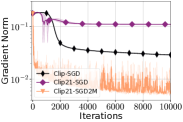
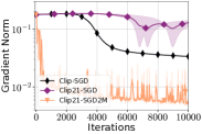
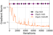
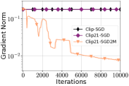
Gaussian, $\tau=10^{-1}$	Gaussian, $\tau=10^{-2}$	Gaussian, $\tau=10^{-3}$	Gaussian, $\tau=10^{-4}$
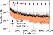
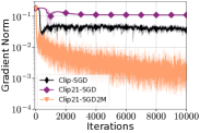
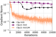
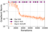
Mini-batch, $\tau=10^{-1}$	Mini-batch, $\tau=10^{-2}$	Mini-batch, $\tau=10^{-3}$	Mini-batch, $\tau=10^{-4}$
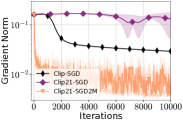
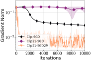
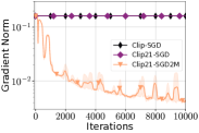
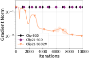
Gaussian, $\tau=10^{-1}$	Gaussian, $\tau=10^{-2}$	Gaussian, $\tau=10^{-3}$	Gaussian, $\tau=10^{-4}$
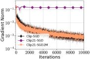
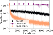
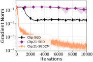
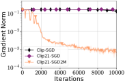
Mini-batch, $\tau=10^{-1}$	Mini-batch, $\tau=10^{-2}$	Mini-batch, $\tau=10^{-3}$	Mini-batch, $\tau=10^{-4}$

Figure 6: Comparison of Clip-SGD, Clip21-SGD, and Clip21-SGD2M ($\hat{\beta}=1$) on logistic regression with non-convex regularization for various the clipping radii $\tau$ with mini-batch and Gaussian-added stochastic gradients on Duke (two first rows) and Leukemia (two last rows).

H.2 Experiments with Neural Networks

H.2.1 Varying Clipping Radius $\tau$

Now we switch to the training of Resnet20 and VGG16 models on CIFAR10 dataset. For all algorithms, we do not use any techniques such as learning rate schedule, warm-up, or weight decay. However, we do tuning of the learning rate for Clip-SGD and Clip21-SGD from $\{10^{-3},10^{-2},10^{-1},10^{0}\}$ and choose the one that gives the highest test accuracy. For Clip21-SGD2M we tune both the learning rate from $\gamma\in\{10^{-3},10^{-2},10^{-1},10^{0}\}$ and the momentum parameter from $\beta\in\{0.1,0.5,0.9\}$ while setting $\hat{\beta}=1$ and choose the pair of $(\gamma,\beta)$ that reaches the highest test accuracy. The batch size for all algorithms is set to $32.$ We compare the performance of algorithms in two cases: when the clipping is applied globally on the whole model and layer-wise.

We observe in Figures˜9, 10, 7 and 8 that the performance of Clip-SGD gets worsen once the clipping radius is small enough. For Clip21-SGD2M is more robust to the choice of $\tau$ and can achieve smaller train loss and test accuracy even when $\tau$ is small.

H.2.2 Results with Additive DP Noise

We consider the training of MLP and CNN models on MNIST dataset varying noise-clipping ration.

We use MLP model with $1$ hidden layer of size $256$ and Tanh activation function. CNN model has $2$ convolution layers with $16$ convolutions each and kernel size $5$ with one max-pooling layer and Tanh activation function. We perform a grid search over the learning rate from $\gamma\in\{10^{-3},\dots,10^{0}\}$ and the clipping radius from $\tau\in\{10^{-4},\dots,10^{-1}\}.$ The aforementioned tuning is performed for each value of the noise-clipping ratio from $\{0.1,0.3,1.0,3.0,10.0\}.$ The momentum parameters are tuned over $\beta\in\{0.5,0.1,0.01\}$ and $\hat{\beta}\in\{0.01,0.1,0.5\}$. We highlight that we do not use the techniques such as a learning rate scheduler although it might improve the performance of algorithms. The batch size for all algorithms is set to $32.$

In Figures˜11, 12, 13 and 14 we demonstrate that Clip-SGD and Clip21-SGD2M always outperform Clip21-SGD. Clip-SGD achieves slightly better accuracy for small noise-clipping ratios $\{0.1,0.3\}$, i.e. weak PD guarantees while Clip21-SGD2M is better for high noise-clipping ratios, i.e. strong DP guarantees.

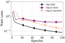
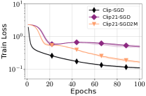
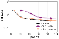
ratio $0.1$	ratio $0.3$	ratio $1.0$

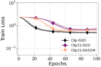
ratio $3.0$

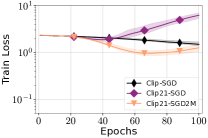
ratio $10.0$

Figure 11: Comparison of Clip-SGD, Clip21-SGD, and Clip21-SGD2M on training CNN model on MNIST dataset varying the noise-clipping ratio.

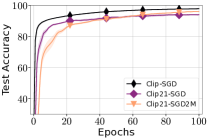
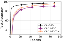
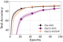
ratio $0.1$	ratio $0.3$	ratio $1.0$

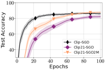
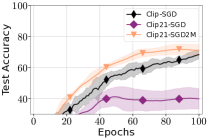
ratio $3.0$	ratio $10.0$

Figure 12: Comparison of Clip-SGD, Clip21-SGD, and Clip21-SGD2M on training CNN model on MNIST dataset varying the noise-clipping ratio.

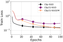
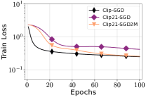
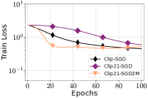
ratio $0.1$	ratio $0.3$	ratio $1.0$

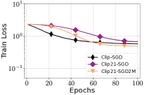
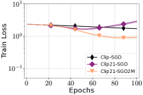
ratio $3.0$	ratio $10.0$

Figure 13: Comparison of Clip-SGD, Clip21-SGD, and Clip21-SGD2M on training MLP model on MNIST dataset varying the noise-clipping ratio.

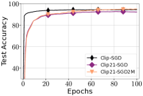
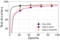
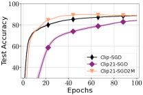
ratio $0.1$	ratio $0.3$	ratio $1.0$

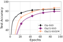
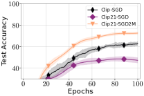
ratio $3.0$	ratio $10.0$

Figure 14: Comparison of Clip-SGD, Clip21-SGD, and Clip21-SGD2M on training MLP model on MNIST dataset varying the noise-clipping ratio.

References

• Abadi et al. (2016) Martin Abadi, Andy Chu, Ian Goodfellow, H Brendan McMahan, Ilya Mironov, Kunal Talwar, and Li Zhang. Deep learning with differential privacy. In Proceedings of the 2016 ACM SIGSAC conference on computer and communications security, 2016.
• Allouah et al. (2024) Youssef Allouah, Anastasia Koloskova, Aymane El Firdoussi, Martin Jaggi, and Rachid Guerraoui. The privacy power of correlated noise in decentralized learning. arXiv preprint arXiv:2405.01031, 2024.
• Arjevani et al. (2023) Yossi Arjevani, Yair Carmon, John C Duchi, Dylan J Foster, Nathan Srebro, and Blake Woodworth. Lower bounds for non-convex stochastic optimization. Mathematical Programming, 2023.
• Balle et al. (2019) Borja Balle, James Bell, Adrià Gascón, and Kobbi Nissim. The privacy blanket of the shuffle model. In Advances in Cryptology–CRYPTO 2019: 39th Annual International Cryptology Conference, Santa Barbara, CA, USA, August 18–22, 2019, Proceedings, Part II 39, 2019.
• Beznosikov et al. (2023) Aleksandr Beznosikov, Samuel Horváth, Peter Richtárik, and Mher Safaryan. On biased compression for distributed learning. Journal of Machine Learning Research, 2023.
• Bonawitz et al. (2017) Keith Bonawitz, Vladimir Ivanov, Ben Kreuter, Antonio Marcedone, H Brendan McMahan, Sarvar Patel, Daniel Ramage, Aaron Segal, and Karn Seth. Practical secure aggregation for privacy-preserving machine learning. In proceedings of the 2017 ACM SIGSAC Conference on Computer and Communications Security, 2017.
• Carmon et al. (2020) Yair Carmon, John C Duchi, Oliver Hinder, and Aaron Sidford. Lower bounds for finding stationary points i. Mathematical Programming, 2020.
• Carmon et al. (2021) Yair Carmon, John C Duchi, Oliver Hinder, and Aaron Sidford. Lower bounds for finding stationary points ii: first-order methods. Mathematical Programming, 2021.
• Chan et al. (2012) TH Hubert Chan, Elaine Shi, and Dawn Song. Optimal lower bound for differentially private multi-party aggregation. In European Symposium on Algorithms, 2012.
• Chang and Lin (2011) Chih-Chung Chang and Chih-Jen Lin. Libsvm: A library for support vector machines. ACM transactions on intelligent systems and technology (TIST), 2011.
• Chaudhuri et al. (2022) Kamalika Chaudhuri, Chuan Guo, and Mike Rabbat. Privacy-aware compression for federated data analysis. In Uncertainty in Artificial Intelligence, 2022.
• Chen et al. (2020) Xiangyi Chen, Steven Z Wu, and Mingyi Hong. Understanding gradient clipping in private sgd: A geometric perspective. Advances in Neural Information Processing Systems, 2020.
• Cutkosky and Mehta (2021) Ashok Cutkosky and Harsh Mehta. High-probability bounds for non-convex stochastic optimization with heavy tails. Advances in Neural Information Processing Systems, 2021.
• Cutkosky and Orabona (2019) Ashok Cutkosky and Francesco Orabona. Momentum-based variance reduction in non-convex sgd. Advances in neural information processing systems, 32, 2019.
• Danilova et al. (2022) Marina Danilova, Pavel Dvurechensky, Alexander Gasnikov, Eduard Gorbunov, Sergey Guminov, Dmitry Kamzolov, and Innokentiy Shibaev. Recent theoretical advances in non-convex optimization. In High-Dimensional Optimization and Probability: With a View Towards Data Science, pages 79–163. Springer, 2022.
• Deng (2012) Li Deng. The mnist database of handwritten digit images for machine learning research. IEEE Signal Processing Magazine, 2012.
• Duchi et al. (2011) John Duchi, Elad Hazan, and Yoram Singer. Adaptive subgradient methods for online learning and stochastic optimization. Journal of machine learning research, 2011.
• Duchi et al. (2018) John C Duchi, Michael I Jordan, and Martin J Wainwright. Minimax optimal procedures for locally private estimation. Journal of the American Statistical Association, 2018.
• Dwork et al. (2014) Cynthia Dwork, Aaron Roth, et al. The algorithmic foundations of differential privacy. Foundations and Trends® in Theoretical Computer Science, 2014.
• Erlingsson et al. (2019) Úlfar Erlingsson, Vitaly Feldman, Ilya Mironov, Ananth Raghunathan, Kunal Talwar, and Abhradeep Thakurta. Amplification by shuffling: From local to central differential privacy via anonymity. In Proceedings of the Thirtieth Annual ACM-SIAM Symposium on Discrete Algorithms, 2019.
• Fatkhullin et al. (2021) Ilyas Fatkhullin, Igor Sokolov, Eduard Gorbunov, Zhize Li, and Peter Richtárik. Ef21 with bells & whistles: Practical algorithmic extensions of modern error feedback. arXiv preprint arXiv:2110.03294, 2021.
• Fatkhullin et al. (2024) Ilyas Fatkhullin, Alexander Tyurin, and Peter Richtárik. Momentum provably improves error feedback! Advances in Neural Information Processing Systems, 2024.
• Gao et al. (2024) Yuan Gao, Rustem Islamov, and Sebastian U Stich. EControl: Fast distributed optimization with compression and error control. In International Conference on Learning Representations, 2024.
• Geyer et al. (2017) Robin C Geyer, Tassilo Klein, and Moin Nabi. Differentially private federated learning: A client level perspective. arXiv preprint arXiv:1712.07557, 2017.
• Ghadimi and Lan (2012) Saeed Ghadimi and Guanghui Lan. Optimal stochastic approximation algorithms for strongly convex stochastic composite optimization i: A generic algorithmic framework. SIAM Journal on Optimization, 2012.
• Gorbunov et al. (2019) Eduard Gorbunov, Darina Dvinskikh, and Alexander Gasnikov. Optimal decentralized distributed algorithms for stochastic convex optimization. arXiv preprint arXiv:1911.07363, 2019.
• Gorbunov et al. (2020a) Eduard Gorbunov, Marina Danilova, and Alexander Gasnikov. Stochastic optimization with heavy-tailed noise via accelerated gradient clipping. Advances in Neural Information Processing Systems, 2020a.
• Gorbunov et al. (2020b) Eduard Gorbunov, Dmitry Kovalev, Dmitry Makarenko, and Peter Richtárik. Linearly converging error compensated sgd. Advances in Neural Information Processing Systems, 2020b.
• Gorbunov et al. (2024) Eduard Gorbunov, Abdurakhmon Sadiev, Marina Danilova, Samuel Horváth, Gauthier Gidel, Pavel Dvurechensky, Alexander Gasnikov, and Peter Richtárik. High-probability convergence for composite and distributed stochastic minimization and variational inequalities with heavy-tailed noise. In Proceedings of the 41st International Conference on Machine Learning, 2024.
• He et al. (2016) Kaiming He, Xiangyu Zhang, Shaoqing Ren, and Jian Sun. Deep residual learning for image recognition. In Proceedings of the IEEE conference on computer vision and pattern recognition, 2016.
• Hegazy et al. (2024) Mahmoud Hegazy, Rémi Leluc, Cheuk Ting Li, and Aymeric Dieuleveut. Compression with exact error distribution for federated learning. In International Conference on Artificial Intelligence and Statistics, 2024.
• Horváth and Richtárik (2020) Samuel Horváth and Peter Richtárik. A better alternative to error feedback for communication-efficient distributed learning. arXiv preprint arXiv:2006.11077, 2020.
• Huang et al. (2023) Xinmeng Huang, Ping Li, and Xiaoyun Li. Stochastic controlled averaging for federated learning with communication compression. arXiv preprint arXiv:2308.08165, 2023.
• Islamov et al. (2024a) Rustem Islamov, Yuan Gao, and Sebastian U Stich. Near optimal decentralized optimization with compression and momentum tracking. arXiv preprint arXiv:2405.20114, 2024a.
• Islamov et al. (2024b) Rustem Islamov, Mher Safaryan, and Dan Alistarh. Asgrad: A sharp unified analysis of asynchronous-sgd algorithms. In International Conference on Artificial Intelligence and Statistics, pages 649–657. PMLR, 2024b.
• Kairouz et al. (2021) Peter Kairouz, H Brendan McMahan, Brendan Avent, Aurélien Bellet, Mehdi Bennis, Arjun Nitin Bhagoji, Kallista Bonawitz, Zachary Charles, Graham Cormode, Rachel Cummings, et al. Advances and open problems in federated learning. Foundations and trends® in machine learning, 2021.
• Karimireddy et al. (2019) Sai Praneeth Karimireddy, Quentin Rebjock, Sebastian Stich, and Martin Jaggi. Error feedback fixes signsgd and other gradient compression schemes. In International Conference on Machine Learning, 2019.
• Karimireddy et al. (2020) Sai Praneeth Karimireddy, Satyen Kale, Mehryar Mohri, Sashank Reddi, Sebastian Stich, and Ananda Theertha Suresh. Scaffold: Stochastic controlled averaging for federated learning. In International conference on machine learning, 2020.
• Kasiviswanathan et al. (2011) Shiva Prasad Kasiviswanathan, Homin K Lee, Kobbi Nissim, Sofya Raskhodnikova, and Adam Smith. What can we learn privately? SIAM Journal on Computing, 2011.
• Khirirat et al. (2023) Sarit Khirirat, Eduard Gorbunov, Samuel Horváth, Rustem Islamov, Fakhri Karray, and Peter Richtárik. Clip21: Error feedback for gradient clipping. arXiv preprint arXiv:2305.18929, 2023.
• Kingma and Ba (2014) Diederik P Kingma and Jimmy Ba. Adam: a method for stochastic optimization. arXiv preprint arXiv:1412.6980, 2014.
• Koloskova et al. (2019) Anastasiia Koloskova, Tao Lin, Sebastian Urban Stich, and Martin Jaggi. Decentralized deep learning with arbitrary communication compression. In Proceedings of the 8th International Conference on Learning Representations, 2019.
• Konečný et al. (2016) Jakub Konečný, H. Brendan McMahan, Felix Yu, Peter Richtárik, Ananda Theertha Suresh, and Dave Bacon. Federated learning: Strategies for improving communication efficiency. In NIPS Private Multi-Party Machine Learning Workshop, 2016.
• Kornilov et al. (2024) Nikita Kornilov, Ohad Shamir, Aleksandr Lobanov, Darina Dvinskikh, Alexander Gasnikov, Innokentiy Shibaev, Eduard Gorbunov, and Samuel Horváth. Accelerated zeroth-order method for non-smooth stochastic convex optimization problem with infinite variance. Advances in Neural Information Processing Systems, 2024.
• Krizhevsky et al. (2009) Alex Krizhevsky, Vinod Nair, and Geoffrey Hinton. Learning multiple layers of features from tiny images. Scientific Report, 2009.
• Levy (2023) Kfir Y. Levy. $\mu^{2}$-sgd: Stable stochastic optimization via a double momentum mechanism, 2023.
• Li and Chi (2023) Boyue Li and Yuejie Chi. Convergence and privacy of decentralized nonconvex optimization with gradient clipping and communication compression. arXiv preprint arXiv:2305.09896, 2023.
• Li et al. (2021) Zhize Li, Hongyan Bao, Xiangliang Zhang, and Peter Richtárik. Page: A simple and optimal probabilistic gradient estimator for nonconvex optimization. In International conference on machine learning, 2021.
• Liu et al. (2022) Mingrui Liu, Zhenxun Zhuang, Yunwen Lei, and Chunyang Liao. A communication-efficient distributed gradient clipping algorithm for training deep neural networks. Advances in Neural Information Processing Systems, 2022.
• Liu et al. (2023) Zijian Liu, Ta Duy Nguyen, Thien Hang Nguyen, Alina Ene, and Huy Nguyen. High probability convergence of stochastic gradient methods. In International Conference on Machine Learning, 2023.
• Madden et al. (2024) Liam Madden, Emiliano Dall’Anese, and Stephen Becker. High probability convergence bounds for non-convex stochastic gradient descent with sub-weibull noise. Journal of Machine Learning Research, 2024.
• Makarenko et al. (2022) Maksim Makarenko, Elnur Gasanov, Rustem Islamov, Abdurakhmon Sadiev, and Peter Richtárik. Adaptive compression for communication-efficient distributed training. arXiv preprint arXiv:2211.00188, 2022.
• Malinovsky et al. (2023) Grigory Malinovsky, Peter Richtárik, Samuel Horváth, and Eduard Gorbunov. Byzantine robustness and partial participation can be achieved simultaneously: Just clip gradient differences. arXiv preprint arXiv:2311.14127, 2023.
• Mangasarian (1995) LO Mangasarian. Parallel gradient distribution in unconstrained optimization. SIAM Journal on Control and Optimization, 1995.
• McMahan et al. (2017a) Brendan McMahan, Eider Moore, Daniel Ramage, Seth Hampson, and Blaise Aguera y Arcas. Communication-efficient learning of deep networks from decentralized data. In Artificial intelligence and statistics, 2017a.
• McMahan et al. (2017b) H Brendan McMahan, Daniel Ramage, Kunal Talwar, and Li Zhang. Learning differentially private recurrent language models. arXiv preprint arXiv:1710.06963, 2017b.
• Mishchenko et al. (2019) Konstantin Mishchenko, Eduard Gorbunov, Martin Takáč, and Peter Richtárik. Distributed learning with compressed gradient differences. arXiv preprint arXiv:1901.09269, 2019.
• Nedic and Ozdaglar (2009) Angelia Nedic and Asuman Ozdaglar. Distributed subgradient methods for multi-agent optimization. IEEE Transactions on Automatic Control, 2009.
• Nemirovski et al. (2009) Arkadi Nemirovski, Anatoli Juditsky, Guanghui Lan, and Alexander Shapiro. Robust stochastic approximation approach to stochastic programming. SIAM Journal on optimization, 2009.
• Noble et al. (2022) Maxence Noble, Aurélien Bellet, and Aymeric Dieuleveut. Differentially private federated learning on heterogeneous data. In Proceedings of The 25th International Conference on Artificial Intelligence and Statistics, 2022.
• Orabona (2019) Francesco Orabona. A modern introduction to online learning. arXiv preprint arXiv:1912.13213, 2019.
• Pagliardini et al. (2024) Matteo Pagliardini, Pierre Ablin, and David Grangier. The ademamix optimizer: Better, faster, older. arXiv preprint arXiv:2409.03137, 2024.
• Papernot et al. (2020) Nicolas Papernot, Steve Chien, Shuang Song, Abhradeep Thakurta, and Ulfar Erlingsson. Making the shoe fit: Architectures, initializations, and tuning for learning with privacy. 2020.
• Pascanu et al. (2013) Razvan Pascanu, Tomas Mikolov, and Yoshua Bengio. On the difficulty of training recurrent neural networks. In Proceedings of the 30th International Conference on International Conference on Machine Learning-Volume 28, 2013.
• Polyak (1964) Boris T Polyak. Some methods of speeding up the convergence of iteration methods. Ussr computational mathematics and mathematical physics, 1964.
• Richtárik et al. (2021) Peter Richtárik, Igor Sokolov, and Ilyas Fatkhullin. Ef21: A new, simpler, theoretically better, and practically faster error feedback. In Advances in Neural Information Processing Systems, 2021.
• Sadiev et al. (2023) Abdurakhmon Sadiev, Marina Danilova, Eduard Gorbunov, Samuel Horváth, Gauthier Gidel, Pavel Dvurechensky, Alexander Gasnikov, and Peter Richtárik. High-probability bounds for stochastic optimization and variational inequalities: the case of unbounded variance. In International Conference on Machine Learning, 2023.
• Sahu et al. (2021) Atal Sahu, Aritra Dutta, Ahmed M Abdelmoniem, Trambak Banerjee, Marco Canini, and Panos Kalnis. Rethinking gradient sparsification as total error minimization. Advances in Neural Information Processing Systems, 2021.
• Seide et al. (2014) Frank Seide, Hao Fu, Jasha Droppo, Gang Li, and Dong Yu. 1-bit stochastic gradient descent and its application to data-parallel distributed training of speech dnns. In Interspeech, 2014.
• Simonyan and Zisserman (2014) Karen Simonyan and Andrew Zisserman. Very deep convolutional networks for large-scale image recognition. arXiv preprint arXiv:1409.1556, 2014.
• Stich and Karimireddy (2019) Sebastian U Stich and Sai Praneeth Karimireddy. The error-feedback framework: Better rates for sgd with delayed gradients and compressed communication. arXiv preprint arXiv:1909.05350, 2019.
• Stich et al. (2018) Sebastian U Stich, Jean-Baptiste Cordonnier, and Martin Jaggi. Sparsified sgd with memory. Advances in neural information processing systems, 2018.
• Streeter and McMahan (2010) Matthew Streeter and H Brendan McMahan. Less regret via online conditioning. arXiv preprint arXiv:1002.4862, 2010.
• Tang et al. (2019) Hanlin Tang, Chen Yu, Xiangru Lian, Tong Zhang, and Ji Liu. Doublesqueeze: Parallel stochastic gradient descent with double-pass error-compensated compression. In International Conference on Machine Learning, 2019.
• Vershynin (2018) Roman Vershynin. High-dimensional probability: An introduction with applications in data science. Cambridge University Press, 2018.
• Wang et al. (2021) Jianyu Wang, Zachary Charles, Zheng Xu, Gauri Joshi, H Brendan McMahan, Maruan Al-Shedivat, Galen Andrew, Salman Avestimehr, Katharine Daly, Deepesh Data, et al. A field guide to federated optimization. arXiv preprint arXiv:2107.06917, 2021.
• Wei et al. (2020) Kang Wei, Jun Li, Ming Ding, Chuan Ma, Howard H Yang, Farhad Farokhi, Shi Jin, Tony QS Quek, and H Vincent Poor. Federated learning with differential privacy: Algorithms and performance analysis. IEEE transactions on information forensics and security, 2020.
• Xie et al. (2020) Cong Xie, Shuai Zheng, Sanmi Koyejo, Indranil Gupta, Mu Li, and Haibin Lin. Cser: Communication-efficient sgd with error reset. Advances in Neural Information Processing Systems, 2020.
• Yau and Wai (2022) Chung-Yiu Yau and Hoi-To Wai. Docom: Compressed decentralized optimization with near-optimal sample complexity. arXiv preprint arXiv:2202.00255, 2022.
• Zhang et al. (2020a) Bohang Zhang, Jikai Jin, Cong Fang, and Liwei Wang. Improved analysis of clipping algorithms for non-convex optimization. In Advances in Neural Information Processing Systems, 2020a.
• Zhang et al. (2020b) Jingzhao Zhang, Tianxing He, Suvrit Sra, and Ali Jadbabaie. Why gradient clipping accelerates training: A theoretical justification for adaptivity. In International Conference on Learning Representations, 2020b.
• Zhang et al. (2020c) Jingzhao Zhang, Sai Praneeth Karimireddy, Andreas Veit, Seungyeon Kim, Sashank Reddi, Sanjiv Kumar, and Suvrit Sra. Why are adaptive methods good for attention models? In Advances in Neural Information Processing Systems, 2020c.
• Zhang et al. (2022) Xinwei Zhang, Xiangyi Chen, Mingyi Hong, Zhiwei Steven Wu, and Jinfeng Yi. Understanding clipping for federated learning: Convergence and client-level differential privacy. In International Conference on Machine Learning, ICML 2022, 2022.