Change-point problem:
Direct estimation using
a geometry inspired reparametrization

Abstract.

Estimation of mean shift in a temporally ordered sequence of random variables with a possible existence of change-point is an important problem in many disciplines. In the available literature of more than fifty years the estimation methods of the mean shift is usually dealt as a two-step problem. A test for the existence of a change-point is followed by an estimation process of the mean shift, which is known as testimator. The problem suffers from over parametrization. When viewed as an estimation problem, we establish that the maximum likelihood estimator (MLE) always gives a false alarm indicting an existence of a change-point in the given sequence even though there is no change-point at all. After modelling the parameter space as a modified horn torus. We introduce a new method of estimation of the parameters. The newly introduced estimation method of the mean shift is assessed with a proper Riemannian metric on that conic manifold. It is seen that its performance is superior compared to that of the MLE. The proposed method is implemented on Bitcoin data and compared its performance with the performance of the MLE.

1. Introduction

Change is an inevitable phenomenon to occur to any physical object in the universe. The time, the amount, and the pattern of changes are of special interest to scientists to understand the dynamics of a system. Sometimes, either the gradual changes are unnoticeable or abrupt changes remain undetected due to the noise present in the data. A sudden change of an unknown amount at an unknown time impacting a system can cause significant problems Hence detection of the occurrence of change, estimation of the change-point and the changed magnitude are problems that are of significant importance and demands a lot of attention. The change-point problem has been one of the most extensively studied non-regular problems in the statistical literature. It arises in a variety of different contexts like environmental sciences Jarušková (1997), ecology, geology, financial markets, astronomy etc. . The retrospective at most one change-point (AMOC) detection problem deals with identifying a time point (which is called the change-point ) in a given temporally-ordered sequence of independent observations, after which the distribution of the random variables undergoes an abrupt change. In contrast, the sequential change-point detection problem deals with the identification of a point in a sequence of independent observations, which are being gathered sequentially, after which the distribution of the random variables has undergone an abrupt change. The sequential change point problem occurs very often in problems of surveillance and quality control. The techniques for dealing with these two different types of change-point problems are substantially different. In this paper, we restrict ourselves to the retrospective AMOC set-up.

In retrospective AMOC detection problems, the presence of a change point in the given sequence of observations needs to be affirmed along with an estimate of the point of change for further decision-making. As an example, consider exoplanet detection techniques that use the photometry measures of periodic dimming of the light intensity of a star caused by a planet passing in front of the star along the line of sight from the observer. If a sequence of independent observations of light intensity is considered the presence of a planet can be suspected if there is a sudden drop in the light intensity or a sudden increase in the light intensity.

In recent times, a lot of discussions have been centered on climate change and its effects. Global warming, broadly defined as an abrupt increase in the earth’s average temperature, is one of the main concerns of climatologists. While the exact cause of global warming is not known the impact of global warming depends crucially on the extent of the rise in the earth’s temperature compared to the historical past. Hence, it is important to have a good estimate of the same. Statistically speaking, not only the detection of the time point of change but also the estimate of the mean shift are of vital interest.

In the context of the retrospective change-point detection problem different authors have enriched the literature with their proposed procedures. Chernoff and Zacks (1964) estimated the current mean of a normal distribution which is subjected to changes in time. Hinkley (1970) discussed inference about the change-point in a sequence of normal random variables with fixed scale parameter. Hawkins (1977) performed the likelihood ratio test and numerical approximation to its limiting distribution. The author established that the asymptotic behavior remains the same whether the pre and post-change parameters are known or not. Yao (1987) gave an approximate distribution of the maximum likelihood estimator (m.l.e) of the change-point. It is shown that the distribution, suitably normalized, of the maximum likelihood estimator based on a large sample converges to the location of the maximum for a two-sided Wiener process when the amount of change in distribution approaches zero. Bhattacharya (1987) derived m.l.e. of a change-point in the distribution of independent random variables for general multi-parameter case. Siegmund (1988) introduces a method based on the likelihood ratio statistic and extends it to the case of independent observations from completely specified distributions belonging to an exponential family. Joint confidence sets for the change-point and the parameters of the exponential family are also considered. A test for change-point was also derived. The discussion by Gombay and Horvath (1990) about the maximum likelihood tests for a change in the mean of independent random variables show that the limit distribution is the Gumbel distribution. Horvath (1993) provided the asymptotic distribution of the maximum likelihood ratio test statistic to check whether the parameters of normal observations had changed at an unknown point. Hartigan et al. (1994) proposed the method of linear estimation of change-point. His argument was based on the limit distribution of the largest deviation between a d-dimensional Ornstein-Uhlenbeck process and the origin. Fotopoulos and Jandhyala (2001) carried out change-point analysis for known parameters based on the application of Weiner-Hopf factorization identity involving the distribution of ascending and descending ladder heights, and the renewal measure in random walks. Mei (2006) considered the problem of minimizing the frequency of false alarms for every possible pre-change distribution when post-change distribution is specified. An asymptotically optimal procedure for one-parameter exponential families is given by the author. Fotopoulos et al. (2010) derived exact computable expressions for the asymptotic distribution of m.l.e of the change-point when a change in the mean occurred at an unknown point of a sequence of time-ordered independent Gaussian random variables. For more details the reader is referred to the monographs of Carlstein et al. (1994), Csörgö and Horváth (1997) and Chen and Gupta (2013).

The related problem of estimation of the current mean or the mean shift has also been studied but not to a large extent. The estimation of mean shift is dependent on the estimation of change-point, which is then considered to be a nuisance parameter. The problem of estimating the current process mean in the presence of change-point is considered by Barnard (1959) and Chernoff and Zacks (1964) in the context of process control. Hawkins et al. (1986) used the least square method for estimating a change in mean. Yashchin (1995) showed that exponentially weighted moving average (EWMA) estimators are optimal in the class of linear estimators for this problem. It is also shown how EWMA estimators can be improved by other general Markovian procedures. The author discussed adaptive schemes that are based on identifying the last change-point and using the resulting last stable segment of data. A common feature of the above-mentioned methodologies is that they achieve their best efficiencies when the sample size is large and the change-point lies near the middle of the sequence of data. They usually do not perform satisfactorily when the change-point is close to either end of the data. A similar observation is made by Bai (1994). The asymptotic behaviour of the likelihood ratio statistic for testing a shift in mean in a sequence of independent normal variates is studied by Yao and Davis (1986). Also, Horvath (1993) reports findings in the same context. Many more authors dealt with the change-point problem from the perspective of testing with univariate (see Page, 1955; Sen and Srivastava, 1975b, a), multivariate (see Srivastava and Worsley, 1986; Gombay and Horvath, 1994; Gombay and Horváth, 1996; Gombay et al., 1996; Jirak et al., 2015), time series (see Shao and Zhang, 2010; Aue and Horváth, 2013) and random field(see Roy et al., 2017) data. Among the recent developments the papers by the following authors are worth mentioning Berkes et al. (2006); Aue et al. (2009); Hušková and Kirch (2008); Keshavarz et al. (2018); Killick et al. (2012); Chen et al. (2015). Note that the mean-shift is equal to zero if there is no change-point in the given data. The reader may refer to the monograph by Wu (2007) which gives some interesting asymptotic results on the distribution of the estimated change-point when the magnitude of the change is small in a linear process.

The most commonly used technique for change point detection is to first perform a test of hypothesis with the null hypothesis being that there is no change in the sequence against the alternative that there is a change point. If this test rejects the null hypothesis of no change at a specified level of significance then an estimation process (such as MLE or CUSUM) is used to estimate the change point. Such an estimator is commonly termed as testimator since its value depends on the result of a test. It may be noted that the value of the testimator depends on the specified level of significance of the test which may be considered as a hyperparameter.

In this paper, we propose a frequentist estimation procedure that does not involve a test of hypothesis and hence is not inherently dependent on the value of the level of significance that is imposed externally.

When the observed sequence of independent random variables is assumed to arise from the same family of distributions then it is interesting to observe that, under some mild regularity conditions, the maximum likelihood estimator (MLE) and the CUSUM estimator of the change point always give a false alarm about presence of a change point even though the data set does not have any. But, on the other hand, if the observed sequence has a change point, it is frequently observed that the MLE performs quite well in identifying the location of the change point. It is observed that the performance of an estimator, e.g. MLE say, has the same efficiency for the true location of the change point at $r$ and $(n-r)$, where $n(>r>0)$ is the sample size and the magnitude of mean shift is non-zero. On the other hand, the change-point locations $r=0$ and $r=n$ both indicate the non-existence of any change-point in the data. In addition, zero mean shift also stands for the non-existence of any change point in the data set. The above facts show that the usual parametrization of the change point problem is non-identifiable. In this paper, we introduce a novel identifiable parametrization of the change point problem. We model the parameter space as a horn-torus with a gradually evolving radius, which is a 3-dimensional conical-manifold (see Ghimenti, 2005, for conical-manifold).

As a consequence, the modelling becomes free from over parametrisation. On this cone-manifold we construct a data-driven graph with the nodes $\{0,1,2,\cdots,n-1\}$ and edges connecting $0$ with $j$ for every $j\neq 0$. These nodes correspond to each possible location of the change point. The structure of the above graph will be used to define the loss function. We introduce an ergodic Markov chain on this graph using an associated transition probability matrix (TPM) whose elements are derived from the values of the likelihood at different nodes. The mode of the stationary distribution of this Markov chain is then used to estimate the location of the change point. The efficiency of the proposed estimator is assessed and compared with the MLE with a suitable metric on this cone-manifold . When there is no change point, our method is able to identify that to a large extent, where as the performance of the testimator is dependent on the specified level of the test. The rest of the paper is structured as follows. Section 2 discusses how the MLE may produce a false alarm of the change-point when the data is free from it. Section 3 provides the unique parametrization of the problem to remove the unwanted redundancy in the parameter space. A new estimation method based on the limiting distribution of a random walk has been introduced in Section 4. The extensive simulation results are reported in Section 5.1, which is followed by Bitcoin data analysis in Section 5.2. The necessary proofs of Lemma 1, Lemma 2 and Theorem 4 are provided in Appendix 7.1,7.2 and 7.3 respectively after the concluding Section 6.

2. A draw-back of the MLE

Let $X$ be a random variable, defined on a probability space $(\Omega,\mathcal{F},P)$, with the cumulative distribution function (c.d.f.) $F_{\mu}(\cdot)$ which is absolutely continuous with respect to the Lebesgue measure $\lambda(\mathbb{R},\mathcal{B}(\mathbb{R}))$ providing a density function $f_{\mu}(\cdot)$ on $\mathbb{R}$ equipped with the Borel $\sigma$-algebra $\mathcal{B}(\mathbb{R}).$ The model parameter $\mu$ belongs to a parameter space $\Xi$ which is an open subset in $\mathbb{R}.$ For a sequence of time-indexed independent random variables $X_{1},X_{2},\cdots,X_{n}$ the change-point problem is:

$$X_{1},X_{2},\cdots,X_{r} \stackrel{{\scriptstyle i.i.d.}}{{\sim}} f_{\mu_{1}}(\cdot)$$

$$\mbox{~~and ~~}X_{r+1},X_{r+2},\cdots,X_{n} \stackrel{{\scriptstyle i.i.d.}}{{\sim}} f_{\mu_{2}}(\cdot),$$ (2.1)

where $(\mu_{1},\mu_{2})\in\Xi\times\Xi$ for some unknown time index $r\in\mathbb{Z}_{n-1}=\left\{0,1,2,\cdots,(n-1)\right\}.$ This formulation involves three parameters $(\mu_{1},\mu_{2},r)$ which are all in general unknown. It may be noted in this parametrization, the case of no change point i.e. $r=0$ can be represented by multiple points in the parameter space $\Xi^{2}\times\mathbb{Z}_{n-1}$ which are either of the form $(\mu_{1}=\mu,\mu_{2}=\mu,r\neq 0)$ or $(\mu_{1},\mu_{2},r=0)$. This gives rise to the problem of non-identifiability in the model which makes estimation of the parameters using methods such as MLE not suitable for use in this set-up.

For carrying out asymptotic analysis in this framework it is often assumed that when a change point is present (i.e. $r\neq 0$), then $r$ is a function of $n$ and $\frac{r}{n}\rightarrow\nu$ as $n\rightarrow\infty$, where $0<\nu<1$. Thus, it is assumed that as $n$ becomes large, the length of both the segments, pre and post the change-point, becomes large too.

Lemma 1 given below points to a major drawback of the MLE when used for the change-point detection problem. It shows that the MLE of $r$ would lie in the set $\mathbb{Z}_{n-1}\setminus\{0\}$ with probability one. Hence, even when no change point is present in the dataset the MLE of $r$ would be different from 0 i.e. it would falsely indicate the presence of a change point, which is generally referred to as a false alarm.

Let $X_{1},X_{2},\cdots,X_{n}$ be independent continuous random variables with density $f_{\mu_{1}}(\cdot)$ for $1\leq i\leq k$ and $f_{\mu_{2}}(\cdot)$ for $k+1\leq i\leq n$ where $k\in\mathbb{Z}_{n-1}$. Let $\lambda_{0}(\mathbf{x})=\displaystyle\prod_{i=1}^{n}f(\mu|x_{i})$ be the likelihood when $k=0$ and $\lambda_{k}(\mathbf{x})={\displaystyle\prod_{i=1}^{k}f(\mu_{1}|x_{i})\prod_{i=k+1}^{n}f(\mu_{2}|x_{i})}$ be that when ${k\in\mathbb{Z}_{n-1}\setminus\{0\}}$.

Lemma 1.

Assume that $\log f(\mu|x)$ is a strictly concave function of $\mu$ and has a unique maxima in the open set $\Xi$. Let $X_{1},X_{2},\cdots,X_{n}$ be i.i.d. $f(\cdot|\mu)$. Then

$$\displaystyle\sup_{\mu\in\Xi}\lambda_{0}(\mathbf{x})<\displaystyle\max_{k\in\mathbb{Z}_{n-1}\setminus\{0\}}\sup_{(\mu_{1},\mu_{2})\in\Xi\times\Xi}\lambda_{k}(\mathbf{x})$$ (2.2)

Thus, $P(\hat{r}_{m}=0)=0$ where $\hat{r}_{m}$ is the MLE of $r$.

Proof: Following Mäkeläinen et al. (1981) the proof is provided in the Appendix 7.1.

Thus, the conventional frequentist approach to the change point problem consists of two stages. Initially, a test of hypothesis $H_{0}:r=0$ against $H_{1}:r\neq 0$ is carried out at an arbitrarily chosen level of significance ($\alpha$) and then depending on the result the second stage of estimation is executed. If $H_{0}$ is not rejected at $100\alpha\%$ level of significance then the data is treated to be coming from a single population and the parameter can be estimated accordingly. If $H_{0}$ is rejected then all three parameters $(\mu_{1},\mu_{2},r)$ are estimated using a suitable technique. The commonly used tests are likelihood ratio test (see Horvath, 1993) or the CUSUM method (see Wu, 2007). To the best of our knowledge, there has been no work reported in the literature that tries to deal with the change point problem purely as an estimation problem in the frequentist setup. In this paper, we introduce a new reformulation of the parameter space of the change point problem that ensures identifiability and allows for the estimation of parameters without taking recourse to a test of hypothesis.

3. An identifiable parametrisation

We have noted in the earlier Section 2, that the parametrization $(\mu_{1},\mu_{2},r)\in\Xi^{2}\times\mathbb{Z}_{n-1}$ is problematic because of non-identifiability. Note that $(\mu_{1},\mu_{2},r)$ can be written as $(\mu_{1},\mu_{1}+(\mu_{2}-\mu_{1}),r)\equiv(\mu_{1},\mu_{1}+\Delta,r)$. Thus we can parametrize using $(\mu_{1},\Delta,r)\in\Xi\times\mathbb{R}\times\mathbb{Z}_{n-1}$. However, this does not eliminate the non-identifiability problem as the case of no change point can be represented by all points in the subset

$$\{(\mu_{1},0,r):\mu_{1}\in\Xi,r\in\mathbb{Z}_{n-1}\setminus\{0\}\}\cup\{(\mu_{1},\Delta,0):\mu_{1}\in\Xi,\Delta\in\mathbb{R}\}$$

Now, observe that in the context of the change point problem, the parameters $\Delta$ (magnitude of change) and $r$ (location of change point) are the parameters of our interest whereas the parameter $\mu_{1}$ is a nuisance parameter.

We now introduce a different parametrization that overcomes the problem of non-identifiability. Let $\tau$ be the left closed right open interval $[0,1)$. Note that an equivalent way of representing a change point at $r$ is to write it as the ratio $\frac{r}{n}\in\tau$.

Let $\Theta$ be the open interval $(-\frac{\pi}{2},\frac{\pi}{2})$ and define $\theta=\arctan(\Delta)\in\Theta.$ To identify the points in $\tau\times\Theta$ which represent the “no-change” situations define a mapping $\mathbf{U}:~\tau\times\Theta\mapsto\mathcal{M}\subset\mathbb{R}^{3}$ as, $\mathbf{U}(t,\theta)=c(t)\mathbb{D}(\mathbf{m}(\theta))e(t)$ where, $c(t)=t(1-t)$, $\mathbb{D}(\mathbf{m}(\theta))$ is a diagonal matrix with diagonal vector $\mathbf{m}(\theta)=(1-\cos\theta,1-\cos\theta,\sin\theta)$ and, $e(t)=[{\cos(2\pi t),\sin(2\pi t),1}]^{T}$. All the points but $\mathbf{0}$ in $\mathcal{M}$ indicates the exact location of the change-point. As explained below $\mathbf{0}=(0,0,0)^{T}$ uniquely identifies the no-change case.

The term $c(t)=t(1-t)$, measures the closeness of the change point to the middle of the sequence. The diagonal vector

$$\mathbf{m}(\theta) = (1-\cos\theta,1-\cos\theta,\sin\theta)$$

$$= \left(1-\frac{1}{\sqrt{1+\Delta^{2}}},1-\frac{1}{\sqrt{1+\Delta^{2}}},\frac{2\Delta}{\sqrt{1+\Delta^{2}}}\right)$$

captures the amount of change with the first two components depending only on the magnitude of the change (i.e. $|\Delta|$) and the third component indicates the sign of the change. Finally, $e(t)=[{\cos(2\pi t),\sin(2\pi t),1}]^{T}$ maps $\tau$ into a unit circle in $(x,y,1)$ plane and the exact location of the change point is mapped to a point on this unit circle. So, $\mathbf{U}(t,\theta)\equiv[u_{1},u_{2},u_{3}]^{T}\equiv\mathbf{u},$ can be represented in matrix notation as

$$\begin{bmatrix}u_{1}(t,\theta)\\ u_{2}(t,\theta)\\ u_{3}(t,\theta)\end{bmatrix}=t(1-t)\begin{bmatrix}1-\cos\theta&0&0\\ 0&1-\cos\theta&0\\ 0&0&\sin\theta\end{bmatrix}\begin{bmatrix}\cos(2\pi t)\\ \sin(2\pi t)\\ 1\end{bmatrix}=t(1-t)\begin{bmatrix}(1-\cos\theta)\cos(2\pi t)\\ (1-\cos\theta)\sin(2\pi t)\\ \sin\theta\end{bmatrix}$$ (3.1)

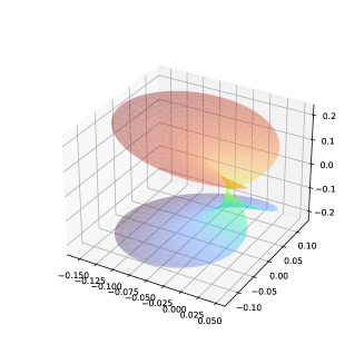
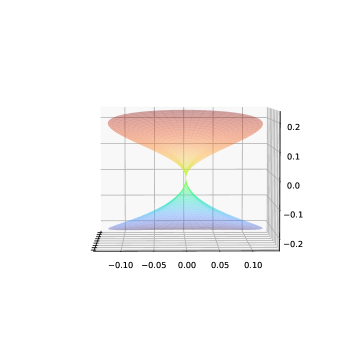
Figure 1. The parameter space $\mathcal{M}$ using Equation-3.1. [from different angles]

It may be noted that $\mathcal{M}\subset\mathbb{R}^{3}$ evolves from the equation of a horn torus
$[(1-\cos\theta)\cos(2\pi t),(1-\cos\theta)\sin(2\pi t),\sin\theta]^{T}$ but with a changing radius $c(t)=t(1-t)$. Note that the no-change situation represented by $t=0$ and/or $\theta=\arctan(\Delta)=0$ is identified to the point $\mathbf{0}=(0,0,0)^{T}\in\mathcal{M}.$ But any other point on $\mathcal{M}$ uniquely describes a certain amount of change corresponding to $\theta\in\Theta$ at a particular location $t\in(0,1)=\tau\setminus\{0\}$. The parameter space can be visualized as a petal-like shape along with its reflection as shown in Figure 1. Now, in the opposite direction, given $\mathbf{u}=(u_{1},u_{2},u_{3})^{T}\neq\mathbf{0}\in\mathcal{M}$ we can obtain $(\theta,t)$ or equivalently $(\Delta,r)$ as follows:

$$\tan(\theta)=\Delta=\frac{u_{3}}{t(1-t)-\sqrt{u_{1}^{2}+u_{2}^{2}}}\mbox{~where~}t=\frac{r}{n}=\frac{1}{2\pi}\arctan\left(\frac{u_{2}}{u_{1}}\right).$$

Because of the point of singularity, $\mathbf{0}$, the surface $\mathcal{M}$ is not a smooth manifold. But it is a special case of a conical manifold, for the definition of which and other properties the reader may look at Ghimenti (2005).

4. Estimation and main result

For a sequence of time-indexed independent random variables $X_{1},X_{2},\cdots,X_{n}$ consider the at-most-one change-point problem as discussed in Section 2. The likelihood function for this problem is

$$\begin{cases}\ell(0)=\displaystyle\max_{\mu\in\Xi}\prod_{i=1}^{n}f(\mu|x_{i})\mbox{~~if~~}\mathbf{u}=\mathbf{0},\\ \ell(k)=\displaystyle\max_{\mu_{1}\in\Xi}\prod_{i=1}^{k}f(\mu_{1}|x_{i})\max_{\mu_{2}\in\Xi}\prod_{i=k+1}^{n}f(\mu_{2}|x_{i})\mbox{~~if~~}\mathbf{u}\neq\mathbf{0}\mbox{~i.e.~}t=\frac{k}{n}\neq 0,\mu_{2}-\mu_{1}\neq 0\end{cases}$$ (4.1)

where, $k\in\{1,2,\ldots,(n-1)\}$ and $\mathbf{u}$ is defined in Equation 3.1. According to the Lemma 1, the index of the maximum of the likelihood sequence $\boldsymbol{\ell}=(\ell(0),\ell(1),\cdots,\ell(n-1))$, always lies in $\mathbb{Z}_{n-1}\setminus\{0\}$, even though there is no change-point in the data. Hence, the MLE of the change-point is

$$\hat{r}_{m}=\arg\max_{k\in\mathbb{Z}_{n-1}}\ell(k)$$ (4.2)

The corresponding estimator of the mean shift is

$$\hat{\Delta}_{\hat{r}_{m}}=\displaystyle\arg\max_{\mu_{2}\in\Xi}\prod_{i={\hat{r}_{m}}+1}^{n}f(\mu_{2}|x_{i})-\displaystyle\arg\max_{\mu_{1}\in\Xi}\prod_{i=1}^{\hat{r}_{m}}f(\mu_{1}|x_{i})$$ (4.3)

As a consequence of the Lemma 1, $\hat{\Delta}_{\hat{r}_{m}}\neq 0$ and $\hat{\mathbf{u}}_{m}\neq\mathbf{0}$ with probability one. To see this, note that $\hat{t}_{m}=\frac{\hat{r}_{m}}{n}\in\tau\setminus\{0\}$ and $\hat{\theta}_{m}=\arctan(\hat{\Delta}_{\hat{r}_{m}})\in(-\frac{\pi}{2},\frac{\pi}{2})$. Hence, the estimated parameter point $\hat{\mathbf{u}}_{m}=\mathbf{U}(\hat{t}_{m},\hat{\theta}_{m})\in\mathcal{M}\setminus\{\mathbf{0}\}.$

To overcome this shortcoming let us consider a graph $\mathcal{G}$ on $\mathbb{Z}_{n-1}$ with a symmetric adjacency matrix $A_{n\times n}$ defined as

$$A=((a_{ij}))=\begin{cases}1\mbox{~~if~~}|i-j|=0\mbox{~~or~~}i\cdot j=0,\\ 0\mbox{~~ otherwise.~~}\end{cases}$$ (4.4)

Hence, all nodes of $\mathcal{G}$ are not only self-connected but each node is connected to $\{0\}$ also. Now to construct a random walk on $\mathcal{G}$, let us first define a transition probability matrix $\mathcal{T}$ depending on both the adjacency matrix $A$ and the likelihood sequence $\boldsymbol{\ell}$ as $\mathcal{T}=[\mathbb{D}(A\boldsymbol{\ell})]^{-1}[A\mathbb{D}(\boldsymbol{\ell})]$ where $\mathbb{D}(\boldsymbol{\ell})$ and $\mathbb{D}(A\boldsymbol{\ell})$ are diagonal matrices with diagonal vectors $\boldsymbol{\ell}$ and $A\boldsymbol{\ell}$ respectively. The definition of $\mathcal{T}$ ensures that each of its row sum equals one. Note that the Markov chain with the transition probability matrix $\mathcal{T}$ is aperiodic, irreducible on a finite state space $\mathbb{Z}_{n-1}$, and hence is ergodic. So, there exists a stationary distribution $\boldsymbol{\pi}=(\pi(0),\pi(1),\cdots,\pi(n-1))^{T}$ satisfying $\boldsymbol{\pi}=\boldsymbol{\pi}\mathcal{T}.$ We now obtain the value of $\pi(k)$ explicitly. For this, denote

$$S=\sum_{i=0}^{n-1}\ell(i)~~\mbox{and}~~S_{i}=\ell(0)+\ell(i)\mbox{~~for~~}i=1,2,\dots,(n-1).$$ (4.5)

Since $\boldsymbol{\pi}=\boldsymbol{\pi}\mathcal{T}$ we get

$$\pi(i) = \pi(0)\frac{\ell(i)}{S}+\pi(i)\frac{\ell(i)}{S_{i}}$$

$$\implies\pi(i) = \frac{S_{i}}{S}\frac{\ell(i)}{\ell(0)}\pi(0)$$

along with the identity $\displaystyle\sum_{i=0}^{n-1}\pi(i)=1.$ Solving we get

$$\pi(0) = \displaystyle\left(1+\sum_{i=1}^{n-1}\frac{S_{i}}{S}\frac{\ell(i)}{\ell(0)}\right)^{-1}$$ (4.6)

$$= S\ell(0)\left(\sum_{i=0}^{n-1}\ell(i)^{2}+2\ell(0)(S-\ell(0))\right)^{-1}\mbox{~using identities from Equation-\ref{likelihood identity}}$$

$$= L(0)\left(\sum_{i=0}^{n-1}L(i)^{2}+2L(0)(1-L(0))\right)^{-1}$$

$$\mbox{~and~}\pi(i) = \frac{\left(L(i)^{2}+L(0)L(i)\right)}{\displaystyle\sum_{i=0}^{n-1}L(i)^{2}+2L(0)(1-L(0))}\mbox{~~ for~}i=1,2,\ldots,(n-1).$$ (4.7)

with $L(i)=\ell(i)/S$ for $i=0,1,2,\ldots,(n-1).$

Now, based on this stationary distribution $\boldsymbol{\pi}$ we propose new estimators for $r$ and $\Delta$ respectively as

$$\hat{r}=\arg\max_{k\in\mathbb{Z}_{n-1}}\pi(k)$$ (4.8)

and

$$\hat{\Delta}=\begin{cases}0\hskip 36.98866pt\mbox{~~if~~}\hat{r}=0,\\ \displaystyle\hat{\Delta}_{\hat{r}_{m}}\hskip 28.45274pt\mbox{~~if~~}\hat{r}=\hat{r}_{m}\in\mathbb{Z}\setminus\{0\}\end{cases}$$ (4.9)

As a consequence, we have $\hat{t}=\frac{\hat{r}}{n}\in\tau$ and $\hat{\theta}=\arctan\hat{\Delta}\in(-\frac{\pi}{2},\frac{\pi}{2})$. Hence the estimated parameter point on $\mathcal{M}$ is $\hat{\mathbf{u}}=\mathbf{U}(\hat{t},\hat{\theta}).$The next Lemma 2 establishes a connection between the MLE, $\hat{r}_{m}$, and the proposed estimator $\hat{r}$.

Lemma 2.

$\hat{r}=0$ or $\hat{r}_{m}$ with probability 1.

Proof: The proof of the lemma is based on a key finding that $\{L(1),L(2),\ldots,L(n-1)\}$ and $\{\pi(1),\pi(2),\ldots,\pi(n-1)\}$ have the same ordering with respect to their magnitudes leading to the only options $\hat{r}=0$ or $\hat{r}_{m}.$ The details of the proof are provided in Appendix 7.2.

Let $\mathbf{p}_{L}$ and $\mathbf{p}_{\pi}$ be the probability vectors representing the marginal distributions of $\hat{r}_{m}$ and $\hat{r}$ for the location of the change point. From Lemma 1 we know that $\mathbf{p}_{L}(0)=P(\hat{r}_{m}=0)=0,$ whereas, in general, $\mathbf{p}_{\pi}(0)=P(\hat{r}=0)\geq 0.$

Lemma 3.

$P(\hat{r}=0)=\displaystyle\sum_{k=1}^{n-1}\delta_{k}~p_{L}(k)$ where $\delta_{k}=P\left(\hat{r}=0|\hat{r}_{m}=k\right).$

Proof: Define the conditional probability , $P(\hat{r}=0|\hat{r}_{m}=k)=\delta_{k}$ and observe that

$$P\left(\hat{r}=0\right) = P\left(\{\hat{r}=0\},\displaystyle\bigcup_{k=1}^{n-1}\{\hat{r}_{m}=k\}\right)=P\left(\displaystyle\bigcup_{k=1}^{n-1}\{\hat{r}=0,\hat{r}_{m}=k\}\right)$$ (4.10)

$$= \displaystyle\sum_{k=1}^{n-1}P\left(\hat{r}=0|\hat{r}_{m}=k\right)P\left(\hat{r}_{m}=k\right)$$

$$= \displaystyle\sum_{k=1}^{n-1}\delta_{k}~p_{L}(k)$$

For ${\mathbf{u}_{1}}=\mathbf{U}({t}_{1},{\theta}_{1})$ and ${\mathbf{u}_{2}}=\mathbf{U}({t}_{2},{\theta}_{2})$ both on $\mathcal{M}$ let us define a metric,

$$d(\mathbf{u}_{1},\mathbf{u}_{2})=\begin{cases}t(1-t)|\theta_{1}-\theta_{2}|\hskip 56.9055pt\mbox{~~if~~}t_{1}=t_{2}=t,\\ t_{1}(1-t_{1})|\theta_{1}|+t_{2}(1-t_{2})|\theta_{2}|\hskip 5.69046pt\mbox{~otherwise,}\end{cases}$$ (4.11)

where the distance between $\mathbf{u}_{1}$ and $\mathbf{0}$ is measured by $t_{1}(1-t_{1})|\theta_{1}|$ and similarly for $\mathbf{u}_{2}.$ It is straightforward to see that $(\mathcal{M},d)$ is a metric space. When $t_{1}\neq t_{2}$ or $\theta_{1}\theta_{2}<0$ then two points are always connected through $\mathbf{0}=(0,0,0).$

Hence this metric is a natural one for the adjacency matrix (see, Equation 4.4) of the embedded graph for the random walk. We will call the metric $d(\cdot,\cdot)$, defined in Equation 4.11 as zero-pass-metric on $\mathcal{M}$. Finally, the accuracy of the MLE $\hat{\mathbf{u}}_{m}=\mathbf{U}(\hat{t}_{m},\hat{\theta}_{m})$ and that of the proposed estimator $\hat{\mathbf{u}}=\mathbf{U}(\hat{t},\hat{\theta})$ are comparable on the parameter space $\mathcal{M}$ with respect to zero-pass-metric $d(\cdot,\cdot)$.

Let us introduce two indicator functions

$$\mathbf{I}_{k}=\begin{cases}1\mbox{~~~~if~~}\hat{r}_{m}=k\\ 0\mbox{~~~~~ otherwise~~}\end{cases}$$ (4.12)

and

$$\mathbf{I}_{k0}=\begin{cases}1\mbox{~~~~if~~}\hat{r}=0\mbox{~when~}\hat{r}_{m}=k\\ 0\mbox{~~~~~ otherwise.~~}\end{cases}$$ (4.13)

Further, define, $\mathbf{I}_{kk}=1-\mathbf{I}_{k0}$, which is the indicator of the event $\hat{r}=k$ when $\hat{r}_{m}=k.$ Let the true value of the parameter $\mathbf{u}=\mathbf{U}(\frac{r}{n},\tan^{-1}\Delta)\in$ $\mathcal{M}$. Now, the loss function for the MLE would be defined as

$$d(\hat{\mathbf{u}}_{m},\mathbf{u})= \displaystyle\sum_{k=1,k\neq r}^{n-1} \left\{\left(\frac{k}{n}\right)\left(1-\frac{k}{n}\right)|\tan^{-1}\hat{\Delta}_{k}|+\left(\frac{r}{n}\right)\left(1-\frac{r}{n}\right)|\tan^{-1}{\Delta}|\right\}\mathbf{I}_{k}$$ (4.14)

$$+ \left(\frac{r}{n}\right)\left(1-\frac{r}{n}\right)|\tan^{-1}\hat{\Delta}_{r}-\tan^{-1}{\Delta}|\mathbf{I}_{r}$$

and similarly the loss function of the proposed estimator is

$$d(\hat{\mathbf{u}},\mathbf{u})= \displaystyle\sum_{k=1,k\neq r}^{n-1} \left\{\left(\frac{k}{n}\right)\left(1-\frac{k}{n}\right)|\tan^{-1}\hat{\Delta}_{k}|\mathbf{I}_{kk}+\left(\frac{r}{n}\right)\left(1-\frac{r}{n}\right)|\tan^{-1}{\Delta}|\right\}\mathbf{I}_{k}$$ (4.15)

$$+ \left(\frac{r}{n}\right)\left(1-\frac{r}{n}\right)\left\{|\tan^{-1}\hat{\Delta}_{r}-\tan^{-1}{\Delta}|\mathbf{I}_{rr}+|\tan^{-1}{\Delta}|\mathbf{I}_{r0}\right\}\mathbf{I}_{r}.$$

Now we compare the risks of $\hat{\mathbf{u}}_{m}$ and $\hat{\mathbf{u}}$ as

$$E(d(\hat{\mathbf{u}}_{m},\mathbf{u})-d(\hat{\mathbf{u}},\mathbf{u}))$$ (4.16)

$$= \displaystyle\sum_{k=1,k\neq r}^{n-1}E\left[\left(\frac{k}{n}\right)\left(1-\frac{k}{n}\right)|\tan^{-1}\hat{\Delta}_{k}|\mathbf{I}_{k}\mathbf{I}_{k0}\right]$$

$$+ \left(\frac{r}{n}\right)\left(1-\frac{r}{n}\right)E\left[\left\{|\tan^{-1}\hat{\Delta}_{r}-\tan^{-1}{\Delta}|-|\tan^{-1}{\Delta}|\right\}\mathbf{I}_{r}\mathbf{I}_{r0}\right]$$

$$= \displaystyle\sum_{k=1,k\neq r}^{n-1}\left[\left(\frac{k}{n}\right)\left(1-\frac{k}{n}\right)E|\tan^{-1}\hat{\Delta}_{k}|p_{L}(k)\delta_{k}\right]$$

$$+ \left(\frac{r}{n}\right)\left(1-\frac{r}{n}\right)\left[\left\{E|\tan^{-1}\hat{\Delta}_{r}-\tan^{-1}{\Delta}|-|\tan^{-1}{\Delta}|\right\}p_{L}(r)\delta_{r}\right]$$

We have

$$E\left[\left(\frac{k}{n}\right)\left(1-\frac{k}{n}\right)|\tan^{-1}\hat{\Delta}_{k}|\mathbf{I}_{k}\mathbf{I}_{k0}\right]=\left(\frac{k}{n}\right)\left(1-\frac{k}{n}\right)E|\tan^{-1}\hat{\Delta}_{k}|p_{L}(k)\delta_{k}$$

because the conditional distribution of $(\hat{\Delta}_{\hat{r}_{m}}|\hat{r}_{m}=k)$ is same as the unconditional distribution $\hat{\Delta}_{k}$ where,

$$\hat{\Delta}_{k}=\displaystyle\arg\max_{\mu_{2}\in\Xi}\prod_{i={k}+1}^{n}f(\mu_{2}|x_{i})-\displaystyle\arg\max_{\mu_{1}\in\Xi}\prod_{i=1}^{k}f(\mu_{1}|x_{i})$$ (4.17)

and $E(\mathbf{I}_{k}\mathbf{I}_{k0})=p_{L}(k)\delta_{k}$ for all $k\in\{1,2,\ldots,(n-1)\}.$

In particular, suppose $X_{1},X_{2},\cdots,X_{n}$ is an independent Gaussian sequence of random variables with known variance $\sigma^{2}$ assumed to be 1. For some $r\in\mathbb{Z}_{n-1}$ (or equivalently $\frac{r}{n}=t\in\tau$), assume that $X_{1},X_{2},\cdots,X_{r}$ are independently distributed $N(\mu_{1},1)$ and $X_{r+1},X_{r+2},\cdots,X_{n}$ are $N(\mu_{2},1)$ random variables. The amount of change or mean shift is $\Delta=\mu_{2}-\mu_{1}=\tan\theta\in\mathbb{R}$ for some $\theta\in\Theta.$ If $\sigma^{2}\neq 1$ then we measure the mean shift $\Delta$ in standard deviation unit i.e. $\Delta=(\mu_{2}-\mu_{1})/\sigma.$

Let $\eta_{n}(r)=\left(\frac{r}{n}\right)\left(1-\frac{r}{n}\right)\left\{E|\tan^{-1}\hat{\Delta}_{r}-\tan^{-1}{\Delta}|-(|\tan^{-1}{\Delta}|+E|\tan^{-1}\hat{\Delta}_{r}|)\right\}p_{L}(r)\delta_{r}.$ We have the following theorem:

Theorem 4.

If $P(\hat{r}=0)\neq 0$ and $d(\cdot,\cdot)$ is the zero-pass-metric defined on the parameter space $\mathcal{M}$, then $E(d(\hat{\mathbf{u}}_{m},\mathbf{u})-d(\hat{\mathbf{u}},\mathbf{u}))\geq\eta_{n}(r)$ where $\eta_{n}(r)\rightarrow 0$ as $n\rightarrow\infty$.

Proof: See Appendix 7.3 for the proof. Also note that, if $P(\hat{r}=0)=0$ then from the Lemma 2 we have $P(\hat{r}=\hat{r}_{m})=1$ which implies $E(d(\hat{\mathbf{u}}_{m},\mathbf{u}))=E(d(\hat{\mathbf{u}},\mathbf{u}))$

Remark 5.

The method of estimating the change-point using the mode of the stationary distribution of a Markov chain with transition probability matrix dependent on the likelihood has not been explored before in the literature to the best of our knowledge. The results discussed in Section 5 shows that this is promising alternative to the MLE. We conjecture that this technique may be useful in other non-regular problems involving both discrete and continuous parameters.

5. Empirical Study

In this section we report the summary of an extensive simulation study and data analysis. We perform comparative studies of the performances of the MLE and the proposed estimator of the change point for different parameter specifications and sample sizes. We also extend our idea to the situation when population variance is fixed but unknown.

Figure 2. Distribution of $\hat{t}_{m}$ and $\hat{t}$ when sample size $n=100$ with no change-point

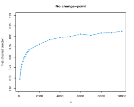
Figure 3. $P(\hat{t}=0)$ with no change-point in the data of different sizes ($n$) from 100 to 10000 .

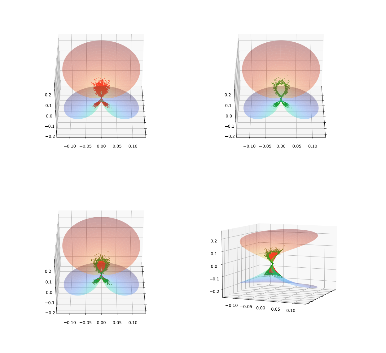
Figure 4. Scatter plot of $\hat{\mathbf{u}}_{m}$ (red, top-left) and $\hat{\mathbf{u}}$ (green, top-right) and overlap of them on $\mathcal{M}$ in the bottom panel from two different angels when there is no change-point in data.

5.1. Simulation Analysis

In Experiment (1), we use simulation to obtain the marginal distributions of $\hat{t}_{m}(\equiv\frac{\hat{r}_{m}}{n})$ and $\hat{t}(\equiv\frac{\hat{r}}{n})$. For this purpose, we perform 10000 iterations of the following: (a) Generate an i.i.d sequence of 100 standard Gaussian random variates and (b) compute the estimates $\hat{t}_{m}$ and $\hat{t}$. The marginal distribution of $\hat{t}_{m}$ and $\hat{t}$ are provided in Figure 2. As expected $\hat{t}_{m}$ has no mass at $t=0$ whereas $\hat{t}$ has a significant mass ($\approx 70\%$) at $t=0.$ We also note that the entire mass of the distribution of $\hat{t}_{m}$ is spread all over the open interval $(0,1)$ in contrast to only $30\%$ of that for $\hat{t}$. Thus the problem of MLE always giving false alarm can be mitigated to a great extent by using $\hat{t}$ instead of $\hat{t}_{m}$. Figure 3 examines $\hat{P}(\hat{t}=0)$ i.e. the estimated probability of $P(\hat{t}=0)$ for different sample sizes varying from from 100 to 10000.

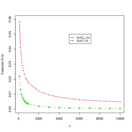
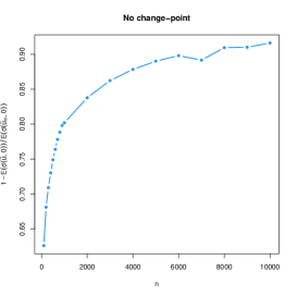
Figure 5. Expected error of the MLE $\hat{\mathbf{u}}_{m}$ and the proposed estimator $\hat{\mathbf{u}}$ (left) and their relative efficiency (RE) (right) for varying sample sizes $n$ from 100 to 100000 when there is no change-point in the data.

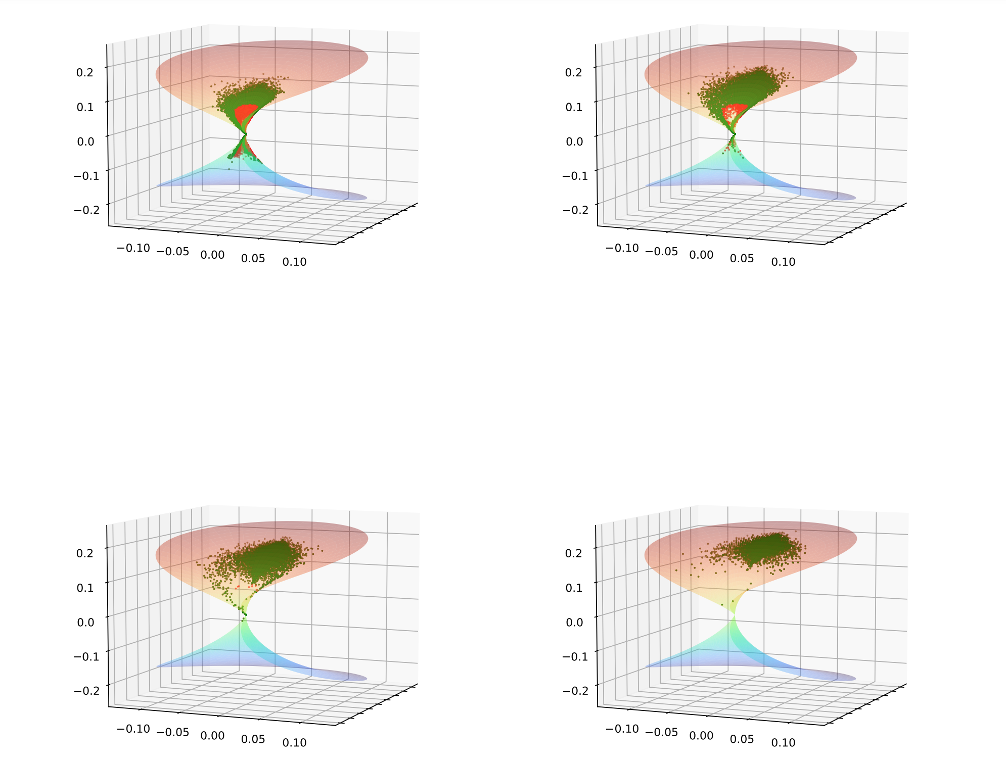
Figure 6. Scatter plot of $\hat{\mathbf{u}}_{m}$ (red) and $\hat{\mathbf{u}}$ (green) on $\mathcal{M}$ for sample size $n=200$ and change-point $r=100$ with $\Delta=0.25(\mbox{top-left}),0.50(\mbox{top-right}),0.75(\mbox{bottom-left}),1.00(\mbox{bottom-right})$ respectively.

In Figure 4 we plot $\hat{\mathbf{u}}_{m}$ (red) and $\hat{\mathbf{u}}$ (green) for 10000 iterations on $\mathcal{M}$ for $n=200$ when no change point is present. As expected the top-left plot of $\hat{\mathbf{u}}_{m}$ shows scattering of points near $\mathbf{0}$ but excluding $\mathbf{0}$. In contrast, the top-right plot of $\hat{\mathbf{u}}$ shows a significant mass at $\mathbf{0}$. The bottom panel shows the overlap of $\hat{\mathbf{u}}_{m}$ and $\hat{\mathbf{u}}$ from different angles and further affirms the above observation.

It is observed from the simulation results that the expected zero-pass metric error (i.e. $E(d(\cdot,\mathbf{u}))$ of $\hat{\mathbf{u}}$ is significantly less than that of $\hat{\mathbf{u}}_{m}$. We define the relative efficiency of $\hat{\mathbf{u}}$ with respect to $\hat{\mathbf{u}}_{m}$ as $RE(\hat{\mathbf{u}},\hat{\mathbf{u}}_{m})=1-\frac{E(d(\hat{\mathbf{u}},\mathbf{u}))}{E(d(\hat{\mathbf{u}}_{m},\mathbf{u}))}$. The top panel of Figure 5 provides plots of ${E(d(\hat{\mathbf{u}},\mathbf{0}))}$ and ${E(d(\hat{\mathbf{u}}_{m},\mathbf{0}))}$ when there is no change point and sample size $n$ varies between 100 to 10000. We find that as sample size increases the expected errors of both $\hat{\mathbf{u}}$ and $\hat{\mathbf{u}}_{m}$ decreases with ${E(d(\hat{\mathbf{u}},\mathbf{0}))}<{E(d(\hat{\mathbf{u}}_{m},\mathbf{0}))}$ for all $n$ in the above range. From the bottom panel it is noted that relative efficiency increases with increasing $n.$

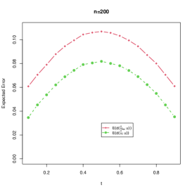
Figure 7. Expected error of the MLE $\hat{\mathbf{u}}_{m}$ and the proposed estimator $\hat{\mathbf{u}}$ (left) and their relative efficiency (RE) (right) for varying locations of the change-point when $n=200$ and $\Delta=0.4$

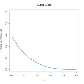
Figure 8. Expected error of the MLE $\hat{\mathbf{u}}_{m}$ and the proposed estimator $\hat{\mathbf{u}}$ (left) and their relative efficiency (RE) (right) for varying amount of mean shift $\Delta$ when sample size $n=100$ with the location of the change point at $r=50.$

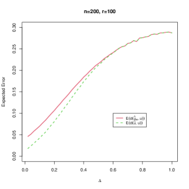
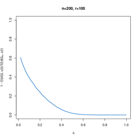
Figure 9. Expected error of the MLE $\hat{\mathbf{u}}_{m}$ and the proposed estimator $\hat{\mathbf{u}}$ (left) and their relative efficiency (RE) (right)for varying amount of mean shift $\Delta$ when sample size $n=200$ with the location of the change point at $r=100.$

In Figure 6 we study the variations in the scatter plots of $\hat{\mathbf{u}}_{m}$ (red) and $\hat{\mathbf{u}}$ (green) on $\mathcal{M}$ with $\Delta$ for 10000 iterations and sample size $n=200$ with change-point at $r=100(\equiv(t=0.5))$. On examining the scatter plots $\Delta=0.25(\mbox{top-left})$, $0.50(\mbox{top-right})$, $0.75(\mbox{bottom-left})$ and $1.00(\mbox{bottom-right})$ we find that the scatter plots of $\hat{\mathbf{u}}_{m}$ and $\hat{\mathbf{u}}$ both move away from $\mathbf{0}$ as $\Delta$ increases. It is further observed from the simulation results that $E(d(\hat{\mathbf{u}}_{m},\mathbf{u}))$ is significantly larger than $E(d(\hat{\mathbf{u}},\mathbf{u}))$ irrespective of the location of the change point. Figure 7 plots $E(d(\hat{\mathbf{u}}_{m},\mathbf{u}))$ and $E(d(\hat{\mathbf{u}},\mathbf{u}))$ in the top panel and relative efficiency of $RE(\hat{\mathbf{u}},\hat{\mathbf{u}}_{m})$ in bottom panel for sample size $n=200$ and mean shift $\Delta=0.4$. We note that the gain in efficiency is maximum when $t$ is close to $0$ or $1.$

In Figures 8 and 9 we examine the variation of $E(d(\hat{\mathbf{u}},\mathbf{u}))$ and $E(d(\hat{\mathbf{u}}_{m},\mathbf{u}))$ with $\Delta$ varying from $0.1$ to $1.0$ for $n=100$ and $n=200$ respectively with change point at $\frac{n}{2}$. We find that $E(d(\hat{\mathbf{u}},\mathbf{u}))\leq E(d(\hat{\mathbf{u}}_{m},\mathbf{u}))$ for all values of $\Delta$ in this range with $\hat{\mathbf{u}}$ out-performing $\hat{\mathbf{u}}_{m}$ significantly for small values of $\Delta.$ The right panels in these two figures show that $RE(\hat{\mathbf{u}},\hat{\mathbf{u}}_{m})$ decreases with $\Delta$ for both values of $n$. Further, it is seen that $RE(\hat{\mathbf{u}},\hat{\mathbf{u}}_{m})$ falls faster for $n=200$ compared to $n=100$.

5.2. Data Analysis

Bitcoin, introduced in 2009 by the anonymous Satoshi Nakamoto, is the first and most well-known cryptocurrency. It operates on a decentralized blockchain network, enabling secure, transparent transactions without intermediaries. With a fixed supply of 21 million coins, Bitcoin is considered a deflationary asset and a digital store of value. Its Proof of Work mechanism ensures transaction validation and network security. As a pioneer in digital finance, Bitcoin has inspired the creation of numerous cryptocurrencies and blockchain applications.

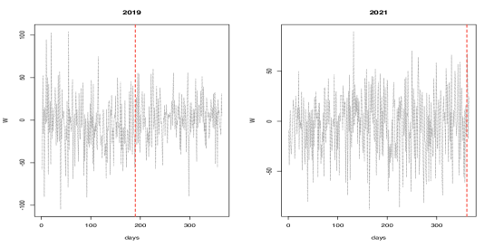
Figure 10. $W$ variable for the bitcoin data in 2019(left) and 2021(right) with location of the change points estimated by the MLE($\hat{r}_{m}$) and denoted by vertical red lines. For the year 2021(right) the MLE is $\hat{r}_{m}=361$ but the proposed estimator shows no indication of change point. On the other hand in the year 2019 the $\hat{r}=\hat{r}_{m}=190.$

To evaluate our proposed change-point detection technique, we utilized a Bitcoin per-minute historical dataset sourced from Kaggle (https://www.kaggle.com/datasets/prasoonkottarathil/btcinusd). This dataset comprises one-minute historical data spanning from January 1, 2017, to March 1, 2022, resulting in 1,860 daily observations after pre-processing. The dataset includes columns for the Unix timestamp, date, symbol, opening price, highest price, lowest price, closing price, cryptocurrency volume, and base currency volume. From this data, we extracted the daily opening price at 00:00 and the closing price at 23:59. Additionally, we calculated the daily average of the lowest and highest prices over the $24\times 60$ minutes. These four variables were then used to construct a new variable for each day,

$$W=\frac{\mbox{Closing Price}-\mbox{Opening Price}}{\mbox{Average High Price}-\mbox{Average Low Price}}$$ (5.1)

It is seen that $W$ is normally distributed with the estimated variance $(\hat{\sigma}_{w}^{2})$ treated as known value ${\sigma}_{w}^{2}$. This is not unrealistic in the cases discussed below as the estimate is obtained on the basis of a large sample size. For the year 2021 with 365 observations of $W$, estimated mean shift is found to have occurred at day $\hat{r}_{m}=361$ as identified by the MLE. But the proposed method does not indicate the presence of any change point with $\hat{r}={0}.$ It refers the corresponding estimates on $\mathcal{M}$ as $\hat{\mathbf{u}}_{m}=(2.939051\times 10^{-3},-2.026942\times 10^{-4},7.428583\times 10^{-3})$ for the MLE and $\hat{\mathbf{u}}=(0,0,0)$ for the proposed estimator. On the contrary for the year 2019 with 365 days the estimate by the MLE and the proposed method coincide at $\hat{r}_{m}=\hat{r}=190.$ Hence the corresponding estimated parameter $\hat{\mathbf{u}}_{m}=\hat{\mathbf{u}}=(-0.010751636,-0.001395871,0.072761484)$ on $\mathcal{M}$. Temporal plot of the data in 2019(left) and 2021(right) are shown in Figure 10 along with location of the change points estimated by the MLE($\hat{r}_{m}$) which is denoted by the vertical red lines.

For the year 2019 the estimated pooled variance $\widehat{Var(W)}=\hat{\sigma}_{w}^{2}=(29.59114)^{2}$ and $(\hat{\mu}_{2}-\hat{\mu}_{1})/\hat{\sigma}_{w}=\hat{\Delta}=0.3079598$ are used to obtained the estimated average loss through parametric bootstrap with 10000 iterations. It is found that for the proposed estimator has the estimated risk $\widehat{E(d(\hat{\mathbf{u}},\cdot))}=0.1381348$ and that of the MLE is $\widehat{E(d(\hat{\mathbf{u}}_{m},\cdot))}=0.1477256.$ Similarly for the year 2021 the estimated pooled variance $\widehat{Var(W)}=\hat{\sigma}_{w}^{2}=(31.22788)^{2}$ and $\hat{\Delta}=0.8110595$ are used to obtained the estimated risk through parametric bootstrap. For the MLE it is observed that the estimated risk is $\widehat{E(d(\hat{\mathbf{u}}_{m},\cdot))}=0.0306724.$ On the other hand under the consideration of no change point $\widehat{Var(W)}=\hat{\sigma}_{w}^{2}=(32.0087)^{2}$ and it is found that the proposed estimator has the estimated risk $\widehat{E(d(\hat{\mathbf{u}},\cdot))}=0.008623216.$

6. Conclusion

The most widely adopted approach to the change point problem for the mean of a distribution has been that of a test for the existence of a change-point, that is followed by an estimation process of the change-point and the mean shift. Thus, in this approach, the estimation process is inextricably intertwined with the testing process. The use of a testing procedure before embarking on the estimation problem is necessitated due to the fact that, if a straightforward maximum likelihood method is utilized, it always shows the presence of a change-point as is proved in this paper. Thus, when there is no change point in the dataset the Maximum likelihood method always raises a false alarm. Since, the change-point problem is inherently an estimation problem, methods not involving a test of hypothesis is desirable. In this paper, we propose a new estimation approach that overcomes the shortcomings of the MLE. A unique reparametrization converts the parameter space to a horn torus with varying radius, which is a conic manifold. The location of the change point and the mean-shift are estimated using a novel random walk based estimation technique. Interestingly, the proposed estimator either indicates non-existence of a change point or coincides with the MLE. This removes the need for an additional step of carrying out a hypothesis test. The efficiency of the newly introduced estimation method of the mean shift is established using a Riemannian metric on the conic manifold. The proposed method is implemented on bitcoin data and its performance is compared with that of the MLE.

7. Appendix

7.1. Proof of the Lemma 1

With out loss of generality let us assume $k\in\mathbb{Z}_{n-1}\setminus\{0\}$. Let us denote

$$\hat{\mu}_{n} = arg\max_{\mu\in\Xi}\prod_{i=1}^{n}f(\mu|x_{i})$$

$$\hat{\mu}_{k,1} = arg\max_{\mu\in\Xi}\prod_{i=1}^{k}f(\mu|x_{i})$$

$$\hat{\mu}_{n-k,2} = arg\max_{\mu\in\Xi}\prod_{i=k+1}^{n}f(\mu|x_{i})$$

Under the assumption of unique maxima of the likelihood as stated in Lemma 1

$$\max_{\mu_{1},\mu_{2}}\prod_{i=1}^{k}f(\mu_{1}|x_{i})\prod_{i=k+1}^{n}f(\mu_{2}|x_{i})$$ (7.1)

$$= \max_{\mu_{1}}\prod_{i=1}^{k}f(\mu_{1}|x_{i})\max_{\mu_{2}}\prod_{i=k+1}^{n}f(\mu_{2}|x_{i})$$

$$= \prod_{i=1}^{k}f(\hat{\mu}_{k,1}|x_{i})\prod_{i=k+1}^{n}f(\hat{\mu}_{n-k,2}|x_{i})$$

$$> \prod_{i=1}^{k}f(\hat{\mu}_{n}|x_{i})\prod_{i=k+1}^{n}f(\hat{\mu}_{n}|x_{i})$$

$$= \max_{\mu}\prod_{i=1}^{n}f(\mu|x_{i})$$

7.2. Proof of the Lemma 2

Let $0<a,b,c$ then $a<b\Leftrightarrow a(a+c)<b(b+c)$. It is immediate that the likelihood sequence $\boldsymbol{\ell}=(\ell(0),\ell(1),\cdots,\ell(n-1))$, and $\mathbf{L}=\boldsymbol{\ell}/S$ have same relative order. Recall from the Equation 4.7 that $\pi(i)\propto L(i)(L(i)+L(0))$ for $i\neq 0$. Now, in particular if we choose $a=L(i)$, $b=L(j)$ and $c=L(0)$ for arbitrary $i\neq j\in\mathbb{Z}_{n-1}\setminus\{0\}$ then $\pi(i)$ and $\pi(j)$ preserve the same order of $L(i)$ and $L(j)$. As a consequence $\{L(1),L(2),\ldots,L(n-1)\}$ and $\{\pi(1),\pi(2),\ldots\pi(n-1)\}$ will preserve the same relative order. But, from the Lemma 1 we get that $L(0)<L(j)$ for all $j=1,2,\ldots,(n-1).$ As a consequence

$$\arg\max_{k\in\mathbb{Z}_{n-1}\setminus\{0\}}\pi(k)=\arg\max_{k\in\mathbb{Z}_{n-1}\setminus\{0\}}\ell(k)=\arg\max_{k\in\mathbb{Z}_{n-1}}\ell(k).$$

Since $P(\pi(0)=\max\{\pi(1),\pi(2),\ldots,\pi(n-1)\})=0$, we can consider the following two possibilities for $\pi(0)$:

$$\mbox{Case-I:~~}\pi(0) < \max\{\pi(1),\pi(2),\ldots,\pi(n-1)\}$$

$$\mbox{ or Case-II:~~ }\pi(0) > \max\{\pi(1),\pi(2),\ldots,\pi(n-1)\}$$

For the Case-I we have $\hat{r}=\hat{r}_{m}$, and for the Case-II we have $\hat{r}=0$.

7.3. Proof of the Theorem 4

Let us define

$$\hat{\Delta}_{k}=\displaystyle\frac{1}{n-{k}}\sum_{i={k}+1}^{n}X_{i}-\displaystyle\frac{1}{k}\sum_{i=1}^{{k}}X_{k}\mbox{~~if~~}{k}\in\mathbb{Z}_{n-1}\setminus\{0\}$$ (7.2)

with

$$E(\hat{\Delta}_{k})=\begin{cases}\frac{n-r}{n-k}\Delta\mbox{\hskip 14.22636pt if ~~}k\leq r\\ \frac{r}{k}\Delta\mbox{\hskip 24.18501pt if ~~}k>r\end{cases}$$

and $Var(\hat{\Delta}_{k})=\frac{n}{k(n-k)}.$ On the other hand, the log likelihood ratio can be expressed as

$$-\log_{e}\left(\frac{\ell(0)}{\ell(k)}\right)=-\log_{e}\left(\frac{L(0)}{L(k)}\right)=\left(\frac{n}{2}\right)\left(\frac{k}{n}\right)\left(1-\frac{k}{n}\right)\left(\hat{\Delta}_{k}\right)^{2}.$$ (7.3)

The scaled mean difference $\sqrt{\frac{k(n-k)}{n}}\hat{\Delta}_{k}$ has variance one with expectation

$$E\left(\sqrt{\frac{k(n-k)}{n}}\hat{\Delta}_{k}\right)=\begin{cases}\sqrt{n\left(\frac{r}{n}\right)\left(1-\frac{r}{n}\right)\left(\frac{k}{r}\right)\left(\frac{n-r}{n-k}\right)}\Delta\mbox{\hskip 14.22636pt if ~~}k\leq r\\ \sqrt{n\left(\frac{r}{n}\right)\left(1-\frac{r}{n}\right)\left(\frac{r}{k}\right)\left(\frac{n-k}{n-r}\right)}\Delta\mbox{\hskip 24.18501pt if ~~}k>r.\end{cases}$$

Now considering the difference of the loss functions

$$E(d(\hat{\mathbf{u}}_{m},\mathbf{u})-d(\hat{\mathbf{u}},\mathbf{u}))$$

$$= \displaystyle\sum_{k=1,k\neq r}^{n-1}\left\{\left(\frac{k}{n}\right)\left(1-\frac{k}{n}\right)E|\tan^{-1}\hat{\Delta}_{k}|\right\}p_{L}(k)\delta_{k}$$

$$+ \left(\frac{r}{n}\right)\left(1-\frac{r}{n}\right)\left\{E|\tan^{-1}\hat{\Delta}_{r}-\tan^{-1}{\Delta}|-|\tan^{-1}{\Delta}|\right\}p_{L}(r)\delta_{r}.$$

$$= \displaystyle\sum_{k=1}^{n-1}\left\{\left(\frac{k}{n}\right)\left(1-\frac{k}{n}\right)E|\tan^{-1}\hat{\Delta}_{k}|\right\}p_{L}(k)\delta_{k}$$

$$+ \left(\frac{r}{n}\right)\left(1-\frac{r}{n}\right)\left\{E|\tan^{-1}\hat{\Delta}_{r}-\tan^{-1}{\Delta}|-(|\tan^{-1}{\Delta}|+E|\tan^{-1}\hat{\Delta}_{r}|)\right\}p_{L}(r)\delta_{r}.$$

$$\equiv \displaystyle\sum_{k=1}^{n-1}\left\{\left(\frac{k}{n}\right)\left(1-\frac{k}{n}\right)E|\tan^{-1}\hat{\Delta}_{k}|\right\}p_{L}(k)\delta_{k}+\eta_{n}(r)$$ (7.5)

If $\mathbf{u}=\mathbf{0}$ i.e. $r=0$ or $\Delta=0$ then the second term of Equation 7.3 is non negative. Now to understand the contribution of the second term of Equation 7.3 when $\mathbf{u}\neq\mathbf{0}$ we focus on the conditional probability

$$\delta_{r} = P(\hat{r}=0|\hat{r}_{m}=r)$$ (7.6)

$$= P(\pi(0)>\pi(r))$$

$$= P(L(0)>L(r)(L(r)+L(0)))$$

$$= P\left(\left(1+\frac{\ell(r)}{\ell(0)}\right)^{-1}>\frac{\ell(r)}{S}\right)$$

$$= P\left(\frac{1}{1+\exp\left\{{0.5}\left(\sqrt{\frac{r(n-r)}{n}}\hat{\Delta}_{r}\right)^{2}\right\}}>\frac{\ell(r)}{S}\right)$$

$$\leq P\left(\frac{1}{1+\exp\left\{{0.5}\left(\sqrt{\frac{r(n-r)}{n}}\hat{\Delta}_{r}\right)^{2}\right\}}\geq\frac{1}{n}\right)\mbox{~since~}\frac{\ell(r)}{S}=\frac{\displaystyle\max_{k}\ell(k)}{\displaystyle\sum_{k=0}^{n-1}\ell(k)}\geq\frac{1}{n}$$

$$= P\left(\hat{\Delta}^{2}_{r}\leq\frac{2\log_{e}(n-1)}{n}\left\{\left(\frac{r}{n}\right)\left(1-\frac{r}{n}\right)\right\}^{-1}\right)$$

The right hand side of the inequality in 7.6 goes to zero as $n\rightarrow\infty$ as

$$\frac{2\log_{e}(n-1)}{n}\rightarrow 0\mbox{~and~}\left\{\left(\frac{r}{n}\right)\left(1-\frac{r}{n}\right)\right\}\rightarrow\nu(1-\nu)$$

Note that $\hat{\Delta}_{r}^{2}$ converges to $\Delta^{2}(\neq 0)$ in probability. As a result, the probability in 7.6 converges to zero, implying $\delta_{r}\rightarrow 0$ as $n\rightarrow\infty$. Since $\hat{\Delta}_{r}\rightarrow\Delta$ in probability and $h_{1}(x)=|\tan^{-1}(x)-\tan^{-1}\Delta|$ and $h_{2}(x)=|\tan^{-1}(x)|$ both are bounded continuous functions, hence by Theorem 5 on page 79 of Chandra (1999) $E|\tan^{-1}\hat{\Delta}_{r}-\tan^{-1}{\Delta}|\rightarrow 0$ and $E|\tan^{-1}\hat{\Delta}_{r}|\rightarrow E|\tan^{-1}{\Delta}|.$ Thus,

$$\left(\frac{r}{n}\right)\left(1-\frac{r}{n}\right)\left\{E|\tan^{-1}\hat{\Delta}_{r}-\tan^{-1}{\Delta}|-(|\tan^{-1}{\Delta}|+E|\tan^{-1}\hat{\Delta}_{r}|)\right\}\rightarrow-2\nu(1-\nu)|\tan^{-1}{\Delta}|$$

Thus, the second term in the Equation 7.3 goes to zero as $n\rightarrow\infty$. Now observe that the first term of 7.3 can be considered as

$$P(\hat{r}=0)\displaystyle\sum_{k=1}^{n-1}\left\{\left(\frac{k}{n}\right)\left(1-\frac{k}{n}\right)E|\tan^{-1}\hat{\Delta}_{k}|\right\}\frac{p_{L}(k)\delta_{k}}{P(\hat{r}=0)}\mbox{~~~when~}P(\hat{r}=0)\neq 0$$

$$= P(\hat{r}=0)E_{\hat{r}_{m}|\hat{r}=0}\left\{\left(\frac{{\hat{r}_{m}}}{n}\right)\left(1-\frac{{\hat{r}_{m}}}{n}\right)|\tan^{-1}\hat{\Delta}_{\hat{r}_{m}}|\right\}\mbox{~ using the Lemma \ref{lm_r_zero}}$$

$$\geq \displaystyle\left\{\left(\frac{M}{n}\right)\left(1-\frac{M}{n}\right)E\left(\tan^{-1}|\hat{\Delta}_{M}|\right)\right\}{p_{L}(M)\delta_{M}}\mbox{~~~where~}M=\arg\max_{k}\left\{p_{L}(k)\delta_{k}\right\}$$

Thus, $E(d(\hat{\mathbf{u}}_{m},\mathbf{u})-d(\hat{\mathbf{u}},\mathbf{u}))\geq\eta_{n}(r)$ where $\eta_{n}(r)\rightarrow 0$ as $n\rightarrow\infty$.

$$\displaystyle\sum_{k=1}^{n-1}\left\{\left(\frac{k}{n}\right)\left(1-\frac{k}{n}\right)E|\tan^{-1}\hat{\Delta}_{k}|\right\}p_{L}(k)\delta_{k}$$

$$= P(\hat{r}=0)E_{\hat{r}_{m}|\hat{r}=0}\left\{\left(\frac{{\hat{r}_{m}}}{n}\right)\left(1-\frac{{\hat{r}_{m}}}{n}\right)|\tan^{-1}\hat{\Delta}_{\hat{r}_{m}}|\right\}$$

$$= P(\hat{r}=0)\displaystyle\sum_{k=1}^{n-1}\left\{\left(\frac{k}{n}\right)\left(1-\frac{k}{n}\right)E\left(\tan^{-1}|\hat{\Delta}_{k}|\right)\right\}\frac{p_{L}(k)\delta_{k}}{P(\hat{r}=0)}\mbox{~~~when~}P(\hat{r}=0)\neq 0$$

$$\geq \displaystyle\left\{\left(\frac{M}{n}\right)\left(1-\frac{M}{n}\right)E\left(\tan^{-1}|\hat{\Delta}_{M}|\right)\right\}{p_{L}(M)\delta_{M}}\mbox{~~~where~}M=\arg\max_{k}\left\{p_{L}(k)\delta_{k}\right\}$$

References

- Aue and Horváth (2013) A. Aue and L. Horváth. Structural breaks in time series. Journal of Time Series Analysis, 34(1):1–16, 2013.
- Aue et al. (2009) A. Aue, L. Horváth, M. Hušková, and S. Ling. On distinguishing between random walk and change in the mean alternatives. Econometric Theory, 25(2):411–441, 2009.
- Bai (1994) J. Bai. Least squares estimation of a shift in linear processes. Journal of Time Series Analysis, 15(5):453–472, 1994.
- Barnard (1959) G. Barnard. Control charts and stochastic processes. Journal of the Royal Statistical Society, Ser.B, 21:239–257, 1959.
- Berkes et al. (2006) I. Berkes, L. Horváth, P. Kokoszka, and Q.-M. Shao. On discriminating between long-range dependence and changes in mean. The annals of statistics, 34(3):1140–1165, 2006.
- Bhattacharya (1987) P. K. Bhattacharya. Maximum likelihood estimation of a change-point in the distribution of independent random variables: general multiparameter case. Journal of Multivariate Analysis, 23(2):183–208, 1987.
- Carlstein et al. (1994) E. Carlstein, H. Müller, and D. Siegmund. Change-point Problems. Number v. 23 in Change-Point Problems. Institute of Mathematical Statistics, 1994. ISBN 9780940600348. URL https://books.google.co.in/books?id=nNSHxxh6TPwC.
- Chandra (1999) T. K. Chandra. A First Course in Asymptotic Theory of Statistics. Narosa Publishing House, India, 1999. ISBN 9788173192609.
- Chen et al. (2015) H. Chen, N. Zhang, et al. Graph-based change-point detection. The Annals of Statistics, 43(1):139–176, 2015.
- Chen and Gupta (2013) J. Chen and A. Gupta. Parametric Statistical Change Point Analysis. Birkhäuser Boston, 2013. ISBN 9781475731316. URL https://books.google.co.in/books?id=7aXzBwAAQBAJ.
- Chernoff and Zacks (1964) H. Chernoff and S. Zacks. Estimating the current mean of a normal distribution which is subjected to changes in time. The Annals of Mathematical Statistics, 35(3):999–1018, 1964.
- Csörgö and Horváth (1997) M. Csörgö and L. Horváth. Limit theorems in change-point analysis. Wiley series in probability and statistics. Wiley, 1997. ISBN 9780471955221. URL https://books.google.co.in/books?id=iyXvAAAAMAAJ.
- Fotopoulos and Jandhyala (2001) S. Fotopoulos and V. Jandhyala. Maximum likelihood estimation of a change-point for exponentially distributed random variables. Statistics & Probability Letters, 51(4):423–429, 2001.
- Fotopoulos et al. (2010) S. B. Fotopoulos, V. K. Jandhyala, and E. Khapalova. Exact asymptotic distribution of change-point mle for change in the mean of gaussian sequences. The Annals of Applied Statistics, 4(2):1081–1104, 06 2010. doi: 10.1214/09-AOAS294. URL https://doi.org/10.1214/09-AOAS294.
- Ghimenti (2005) M. Ghimenti. Geodesics in conical manifolds. Topological Methods in Nonlinear Analysis, 25(2):235–261, 2005.
- Gombay and Horvath (1990) E. Gombay and L. Horvath. Asymptotic distributions of maximum likelihood tests for change in the mean. Biometrika, 77(2):411–414, 1990.
- Gombay and Horvath (1994) E. Gombay and L. Horvath. An application of the maximum likelihood test to the change-point problem. Stochastic Processes and their Applications, 50(1):161–171, 1994.
- Gombay and Horváth (1996) E. Gombay and L. Horváth. Approximations for the time of change and the power function in change-point models. Journal of Statistical Planning and Inference, 52(1):43–66, 1996.
- Gombay et al. (1996) E. Gombay, L. Horvath, et al. On the rate of approximations for maximum likelihood tests in change-point models. Journal of Multivariate Analysis, 56(1):120–152, 1996.
- Hartigan et al. (1994) J. Hartigan et al. Linear estimators in change point problems. The Annals of Statistics, 22(2):824–834, 1994.
- Hawkins et al. (1986) D. Hawkins, A. Gallant, and W. Fuller. A simple least squares method for estimating a change in mean. Communications in Statistics-Simulation and Computation, 15(3):523–530, 1986.
- Hawkins (1977) D. M. Hawkins. Testing a sequence of observations for a shift in location. Journal of the American Statistical Association, 72(357):180–186, 1977.
- Hinkley (1970) D. V. Hinkley. Inference about the change-point in a sequence of random variables. Biometrika, 57(1):1–17, 1970.
- Horvath (1993) L. Horvath. The maximum likelihood method for testing changes in the parameters of normal observations. The Annals of Statistics, 21(2):671–680, 06 1993. doi: 10.1214/aos/1176349143. URL https://doi.org/10.1214/aos/1176349143.
- Hušková and Kirch (2008) M. Hušková and C. Kirch. Bootstrapping confidence intervals for the change-point of time series. Journal of Time Series Analysis, 29(6):947–972, 2008.
- Jarušková (1997) D. Jarušková. Some problems with application of change-point detection methods to environmental data. Environmetrics: The official journal of the International Environmetrics Society, 8(5):469–483, 1997.
- Jirak et al. (2015) M. Jirak et al. Uniform change point tests in high dimension. The Annals of Statistics, 43(6):2451–2483, 2015.
- Keshavarz et al. (2018) H. Keshavarz, C. Scott, and X. Nguyen. Optimal change point detection in gaussian processes. Journal of Statistical Planning and Inference, 193:151–178, 2018.
- Killick et al. (2012) R. Killick, P. Fearnhead, and I. A. Eckley. Optimal detection of changepoints with a linear computational cost. Journal of the American Statistical Association, 107(500):1590–1598, 2012.
- Mäkeläinen et al. (1981) T. Mäkeläinen, K. Schmidt, and G. P. Styan. On the existence and uniqueness of the maximum likelihood estimate of a vector-valued parameter in fixed-size samples. The Annals of Statistics, pages 758–767, 1981.
- Mei (2006) Y. Mei. Sequential change-point detection when unknown parameters are present in the pre-change distribution. The Annals of Statistics, 34(1):92–122, 2006.
- Page (1955) E. Page. A test for a change in a parameter occurring at an unknown point. Biometrika, 42(3/4):523–527, 1955.
- Roy et al. (2017) S. Roy, Y. Atchadé, and G. Michailidis. Change point estimation in high dimensional markov random-field models. Journal of the Royal Statistical Society: Series B (Statistical Methodology), 79(4):1187–1206, 2017.
- Sen and Srivastava (1975a) A. Sen and M. S. Srivastava. Some one-sided tests for change in level. Technometrics, 17(1):61–64, 1975a.
- Sen and Srivastava (1975b) A. Sen and M. S. Srivastava. On tests for detecting change in mean. The Annals of statistics, pages 98–108, 1975b.
- Shao and Zhang (2010) X. Shao and X. Zhang. Testing for change points in time series. Journal of the American Statistical Association, 105(491):1228–1240, 2010. doi: 10.1198/jasa.2010.tm10103.
- Siegmund (1988) D. Siegmund. Confidence sets in change-point problems. International Statistical Review/Revue Internationale de Statistique, pages 31–48, 1988.
- Srivastava and Worsley (1986) M. Srivastava and K. J. Worsley. Likelihood ratio tests for a change in the multivariate normal mean. Journal of the American Statistical Association, 81(393):199–204, 1986.
- Wu (2007) Y. Wu. Inference for change point and post change means after a CUSUM test, volume 180. Springer Science & Business Media, 2007.
- Yao (1987) Y.-C. Yao. Approximating the distribution of the maximum likelihood estimate of the change-point in a sequence of independent random variables. Ann. Statist., 15(3):1321–1328, 09 1987. doi: 10.1214/aos/1176350509. URL https://doi.org/10.1214/aos/1176350509.
- Yao and Davis (1986) Y.-C. Yao and R. A. Davis. The asymptotic behavior of the likelihood ratio statistic for testing a shift in mean in a sequence of independent normal variates. Sankhyā: The Indian Journal of Statistics, Series A, pages 339–353, 1986.
- Yashchin (1995) E. Yashchin. Estimating the current mean of a process subject to abrupt changes. Technometrics, 37(3):311–323, 1995.