Iterative Procedure for Non-Linear Fractional Integro-Differential Equations via Daftardar–Jafari Polynomials

Abstract

In this paper, we introduce a novel approach called the Iterative Aboodh Transform Method (IATM) which utilizes Daftardar–Jafari polynomials for solving non-linear problems. Such method is employed to derive solutions for non-linear fractional partial integro-differential equations (FPIDEs). The key novelty of the suggested method is that it can be used for handling solutions of non-linear FPIDEs in a very simple and effective way. More precisely, we show that Daftardar–Jafari polynomials have simple calculations as compared to Adomian polynomials with higher accuracy. The results obtained within the Daftardar–Jafari polynomials are demonstrated with graphs and tables, and the IATM’s absolute error confirms the higher accuracy of the suggested method.

Keywords: Caputo operator; Aboodh transformation; Iterative Method; Daftardar–Jafari Polynomials.

1 Introduction

Fractional partial integro-differential equations (FPIDEs), which incorporate both integrals and fractional derivatives, play a crucial role in the study of fractional calculus. A significant aspect of FPIDEs is the application of fractional specifications, which has become one of the essential mathematical tools for modelling and analysing real-world problems in natural sciences, engineering, and technology [1, 2, 3, 4]. Due to the non-local property of fractional derivative operators, the study on FPIDEs is highly non-trivial and challenging. Nonetheless, various researchers have made significant strides in studying FPIDEs analytical and numerically, here we briefly recall some results from the literature. Hassan et al. [5] employed the Chebyshev Wavelet Method (CWM) to tackle higher-order fractional integro-differential equations (FIDEs), demonstrating the method’s potential in handling complex fractional dynamics. Mohyud-Din et al. [6] applied the CWM to non-linear FIDEs, showcasing its versatility across different types of equation. To derive analytical solutions for FPIDEs, Hussain et al. [7] utilized the variation iteration approach, while Mittal et al. [8] implemented the Adomian decomposition method to solve FPIDEs. Additionally, Awawdeh et al. [9] employed the homotopy analysis method to derive analytical solutions for linear FPIDEs. Eslahchi et al. explored the Jacobi method for solving non-linear FPIDEs, investigating stability and convergence in their analysis [10]. Zhao et al. [11] introduced a piecewise polynomial collocation approach to address FPIDEs with weakly singular kernels, illustrating an innovative numerical strategy. Rawashdeh proposed a numerical method leveraging polynomial splines for effective numerical solutions of FPIDEs [12]. Furthermore, Unhale et al. [13] suggested a collocation method using shifted Legendre polynomials and Chebyshev polynomials to solve non-linear FPIDEs, while Avazzadeh et al. combined Legendre wavelets with a fractional integration operational matrix in a hybrid approach [14]. Lastly, Arshed applied the B-spline method to find solutions to linear FPIDEs [15], and Dehestani et al. introduced the collocation method for the numerical simulation of FPIDEs [16]. This evolving body of research underscores the growing significance of FPIDEs and the diverse methodologies being developed to address them effectively.

On the other hand, It is also worth mentioning a special type of fractional equations, which are known as Stochastic fractional integro-differential equations (SFIDEs). SFIDEs are mathematical models that integrate the principles of stochastic processes, fractional calculus, and integral equations, enabling the representation of systems with inherent randomness and memory effects. SFIDEs are particularly useful in fields such as finance, physics, and biology, where they model phenomena characterized by unpredictable behaviour and long-term dependencies, such as stock price movements or the diffusion of particles in complex media. References and related discussions can be found in Mirzaee et al.[17, 18, 19, 20], Solhi et al. [21], Alipour and Mirzaee [22], Mirzaee and Alipour [23], Samadyar and Mirzaee[24].

In the current study, we introduce the Iterative Aboodh transform method (IATM) to obtain the approximate solution of non-linear FPIDEs. To represent fractional derivatives, the Caputo derivative operator is utilised and the Daftardar–Jafari polynomials from [25, 26] are used to express the non-linear terms in each targeted problem. The Daftardar–Jafari polynomials have a straightforward implementation in a given infinite series form that can provide the sufficient degree of accuracy. The solutions of three examples are then illustrated in details to confirm the reliability of the suggested technique. Using MAPLE software, a very simple algorithm of the present method is constructed with the aid of Daftardar–Jafari polynomials for non-linear FPIDEs.

The IATM is comparably simple in the sense that it involves fewer calculations, which makes it suitable for extending to the study on solutions of other FPIDEs and their associated systems. More precisely, this research work has the following multiple advantages:

• We successfully achieve highly accuracy with the same number of iterations and parameters than the results recently published in Khan et al. [27] and the related works cited therein.

• The non-linear terms are controlled by Daftardar–Jafari polynomials, which allow us to incorporate non-linearity directly into a more simple algebraic expression without involving derivatives as compare with Adomian polynomials and He’s polynomials.

• The mathematical model investigated has significant physical interpretation on various subjects, such as the heat flow in materials with memory and the mechanics of viscoelasticity. Reference [28] and the references cited therein will provide further insights into these applications, which can illustrate the model’s utility for understanding complex material behaviours.

• We deal with one of the most commonly used fractional derivative operators, known as the Caputo derivative, which can improve the modelling accuracy for describing physical phenomena with viscoelastic forces; refer to equation (3.1).

• We believe that the newly proposed IATM may bring insights on the study of other related fractional equations, which include SFIDEs as discussed before. Further investigations will be carried out in subsequent research projects later.

The rest of the paper is organised as follows. In Section 2, we give the definitions of some fundamental concepts related to fractional calculus and operators. In Section 3, we introduce the IATM for solving non-linear FPIDEs. In Section 4, we provide the details on the numerical implementation of the proposed method, with the showcases of some specific problems and their solutions. In Section 5, we discuss the results of our numerical experiments and present some further implications. Finally, we conclude in Section 6 with a summary of findings and reflections on the applicability of the proposed approach.

2 Basic Definitions

In this section, we provide some definitions that are essential for implementing the iterative scheme. Interested readers are encouraged to consult the references [29, 30, 31, 32, 33, 34] for further information. To begin with, we define the Caputo operator for fractional derivatives.

Definition 1.

The Caputo operator for fractional derivatives of order ${{{{\alpha}}}}$ is given by

$$D_{{{{{t}}}}}^{{{{{\alpha}}}}}{{{{u}}}}({{{{x}}}},{{{{t}}}})=\frac{1}{\Gamma({{{j}}}-{{{{\alpha}}}})}\int^{{{{t}}}}_{0}({{{{t}}}}-{{{{t}}}}_{o})^{{{{j}}}-{{{{\alpha}}}}-1}\frac{\partial^{{{j}}}{{{{u}}}}({{{{x}}}},{{{{t}}}})}{\partial{{{{t}}}}^{{{j}}}}d{{{{t}}}},\leavevmode\nobreak\ \leavevmode\nobreak\ \leavevmode\nobreak\ \leavevmode\nobreak\ if\leavevmode\nobreak\ \leavevmode\nobreak\ \leavevmode\nobreak\ {{{j}}}-1<{{{{\alpha}}}}\leq{{{j}}}.$$ (2.1)

If ${{{{\alpha}}}}={{{j}}}$ for ${{{j}}}\in\mathbb{N}$, then the operator $D_{{{{{t}}}}}^{{{{{\alpha}}}}}$ is reduced to the ordinary time derivative

$$D_{{{{{t}}}}}^{{{{{\alpha}}}}}{{{{u}}}}({{{{x}}}},{{{{t}}}})=\frac{\partial^{{{j}}}{{{{u}}}}({{{{x}}}},{{{{t}}}})}{\partial{{{{t}}}}^{{{j}}}}.$$

Next, we introduce the well-known Laplace transform $\mathcal{L}(\cdot)$ and its interactions with Caputo operator.

Definition 2.

For a function $g({{{{{t}}}}})$, the Laplace transform is given by

$${G(s)}=\mathcal{L}[{g({{{{t}}}})}]=\int_{0}^{\infty}e^{-s{{{t}}}}{g}({{{{{t}}}}})d{{{{t}}}}.$$

We further have the following identities involving Laplace transform and Caputo operator:

$$\begin{split}\mathcal{L}(D_{{{{t}}}}^{{{{{\alpha}}}}}{{{{u}}}}({{{{t}}}}))&=s^{{{{\alpha}}}}\mathcal{L}[{{{{u}}}}({{{{t}}}})]-\sum_{k=0}^{{j}-1}s^{{{{{{\alpha}}}}}-j-1}U^{k}(0^{+}),\ \ {j}-1<{{{{\alpha}}}}\leq{j},\ \ \forall{j}\in\mathbb{N}.\\ \mathcal{L}(D_{{{{t}}}}^{{{{{\alpha}}}}}{{{{u}}}}({{{{t}}}}))&=s^{{{{\alpha}}}}U(s)-s^{{{{{\alpha}}}}-1}U(0),\ \ \ 0<{{{{\alpha}}}}\leq{1}\ \ \ \ {for}\ \ {j}=1.\end{split}$$

We now introduce the Daftardar–Jafari polynomials (also known as the Daftardar–Jafari method) which is used for expressing the non-linear term in an approximate problem. Details are given as follows.

Definition 3.

Suppose that $u(x,t)$ is a solution to the following functional equation

$$u(x,t)=N(u(x,t))+f(x,t),$$

where $N(\cdot)$ is a non-linear operator between Banach spaces $\mathcal{B}_{1}$ and $\mathcal{B}_{2}$, and $f$ is a given function. We are looking for $u(x,t)$ in a series form

$$u(x,t)=\sum_{j=0}^{\infty}u_{j}(x,t).$$

The non-linear operator $N(\cdot)$ can then be decomposed as follows:

$$N\left(\sum_{{j}=0}^{\infty}{{{{{u}}}}_{j}({{{{x}}}},{{{{t}}}})}\right)=N({{{{{u}}}}_{0}({{{{x}}}},{{{{t}}}})})+\sum_{{j}=0}^{\infty}\bigg{[}{N}\bigg{(}\sum_{i=0}^{{j}}{{{{u}}}}_{i}({{{{x}}}},{{{{t}}}})\bigg{)}-{N}\bigg{(}\sum_{i=0}^{{j}-1}{{{{u}}}}_{i}({{{{x}}}},{{{{t}}}})\bigg{)}\bigg{]},$$ (2.2)

where $u_{0}:=f$ and $u_{1}:=N(u_{0})$ are respectively the Daftardar–Jafari polynomials $u_{j}$ when $j=0$ and $\j=1$. For $j\geq 2$, the Daftardar–Jafari polynomials $u_{j}$ with respect to the solution $u$ are given by

$$u_{j}:=N(u_{0}+\cdots+u_{j-1})-N(u_{0}+\cdots+u_{j-2}).$$

Throughout this paper, the Daftardar–Jafari polynomials are utilized to represent the non-linear terms in various problems, which will be explained in Section 3 and Section 4 later.

Lastly, we introduce the Aboodh transform (AT) and some related identities.

Definition 4.

Given $M\in(0,\infty)$ and $k_{1},k_{2}\in(0,\infty]$, we define a set of functions $\mathbf{S}:=\mathbf{S}(M,k_{1},k_{2})$ as follows

$${\mathbf{S}}=\{{{{{u}}}}({{{{t}}}}):|{{{{u}}}}({{{{t}}}})|<Me^{-st},\ \ t\geq 0,\ \ k_{1}\leq s\leq k_{2}\}.$$

For any $u\in\mathbf{S}$, the Aboodh transform (AT) $\mathcal{A}[u]$ of $u$ is given by

$${k}({s}):=\mathcal{A}\left[{{{{{u}}}}}\right]=\frac{1}{s}\int_{0}^{\infty}{{{{{u}}}}}({{{{{t}}}}})e^{-s{{{{{t}}}}}}{d}{{{{{t}}}}},\ \ {{{{{t}}}}}\geq 0,\ \ {{{k}}}_{1}\leq{s}\leq{{{k}}}_{2}.$$

The operator $\mathcal{A}$ enjoys the following properties:

• $\mathcal{A}\left[{{{{{{u}}}}}^{{}^{\prime}}}({{{{{t}}}}})\right]=s\mathcal{A}[u](s)-\frac{{{{{u}}}}(0)}{s},$

• $\mathcal{A}\left[{{{{{{u}}}}}^{{}^{\prime\prime}}}({{{{{t}}}}})\right]=s^{2}\mathcal{A}[u](s)-\frac{{{{{{{u}}}}}^{{}^{\prime}}}(0)}{s}-{{{{{u}}}}(0)},$
  ⋮

• $\mathcal{A}\left[{{{{{{u}}}}}^{(n)}}({{{{{t}}}}})\right]=s^{n}\mathcal{A}[u](s)-\sum_{{j}=0}^{n-1}\frac{{{{{{{u}}}}}^{(n)}}(0)}{s^{2}-n+j}$.

Furthermore, if $a$ and $b$ are constants and ${{{{u}}}}({{{{t}}}}),{{{{v}}}}({{{{t}}}})\in\mathbf{S}$, then we have

$$\mathcal{A}\left[a{{{{{{u}}}}}}({{{{{t}}}}})\pm b{{{{v}}}}({{{{t}}}})\right]=a\mathcal{A}\left[{{{{{{u}}}}}}({{{{{t}}}}})\right]\pm b\mathcal{A}\left[{{{{v}}}}({{{{t}}}})\right].$$

We also define $\mathcal{A}^{-1}$ as follows. If $f(t)$ is piecewise continuous and of exponential order for $t\geq 0$ such that $\mathcal{A}[f(t)]=F(s)$, then $f(t)$ is called inverse Aboodh transform of $F(s)$ and we write $\mathcal{A}^{-1}[f(s)]=F(t)$.

One of the important applications of AT is for converting Caputo fractional differential operators into algebraic equations. Specifically, for $\alpha\in(0,1]$, the AT of $D^{\alpha}_{{{{{{t}}}}}}{{{{u}}}}$ is defined as

$$\mathcal{A}[D^{\alpha}_{{{{{{t}}}}}}{{{{u}}}}]({{{{{x}}}}},{{{{{s}}}}})={{s}}^{\alpha}\mathcal{A}[{{{{{u}}}}}]({{{{{x}}}}},{{s}})-{{s}}^{\alpha-2}\mathcal{A}[{{{{u}}}}]({{{{{x}}}}},0).$$

3 IATM for non-linear FPIDEs

In this section, we introduce the new approach known as the Iterative Aboodh Transform Method (IATM). In order to understand IATM, we consider the following non-linear FPIDEs

$$\begin{split}{{D}^{{{{\alpha}}}}_{{{{{t}}}}}{{{{{u}}}}({{{{x}}}},{{{{t}}}})}}+{{{{{u}}}}({{{{x}}}},{{{{t}}}})}{\frac{\partial}{{\partial}{{{{{x}}}}}}}{{{{{u}}}}({{{{x}}}},{{{{t}}}})}=\int_{0}^{{{{{t}}}}}\!\left({{{{{t}}}}}-{q}\right)^{{{{{\alpha}}}}-1}\,{\frac{\partial^{2}}{{\partial}{{{{{x}}}}}^{2}}}{{{{{u}}}}({{{{x}}}},{{{{t}}}})}{\rm d}q+f({{{{x}}}},{{{{t}}}})\ \ \ {{{{\alpha}}}}\in(0,1]\end{split}$$ (3.1)

where $f({{{{x}}}},{{{{t}}}})$ is a given source term and ${D}^{{{{\alpha}}}}_{{{{{t}}}}}$ is the Caputo type fractional order derivative as defined in (2.1). The above equation (3.1) is equipped with initial and boundary conditions

$${{{{u}}}}({{{{x}}}},0)=g({{{{x}}}}),\ \ {{{{u}}}}(0,{{{{t}}}})={{{{u}}}}(L,{{{{t}}}})=0.$$

Applying Aboodh transform (AT) on equation (3.1), we get

$$\begin{split}\mathcal{A}[{D}^{{{{\alpha}}}}_{{{{{t}}}}}{{{{u}}}}({{{{x}}}},{{{{t}}}})]=\mathcal{A}\left[\int_{0}^{{{{{t}}}}}\!\left({{{{{t}}}}}-{q}\right)^{{{{{\alpha}}}}-1}\,{\frac{\partial^{2}}{{\partial}{{{{x}}}}^{2}}}{{{{{u}}}}({{{{x}}}},{{{{t}}}})}{\rm d}q-{{{{{u}}}}({{{{x}}}},{{{{t}}}})}{\frac{\partial}{{\partial}{{{{x}}}}}}{{{{{u}}}}({{{{x}}}},{{{{t}}}})}+f({{{{x}}}},{{{{t}}}})\right].\end{split}$$

Using the algebraic property of AT on fractional derivatives, equation (3.1) can be rewritten as follows

$${s^{{{{\alpha}}}}}\mathcal{A}\left[{{{{{{u}}}}}({{{{x}}}},{{{{t}}}})}\right]=s^{{{{{\alpha}}}}-2}{{{{{u}}}}}({{{{x}}}},0)+\mathcal{A}\left[\int_{0}^{{{{{t}}}}}\!\left({{{{{t}}}}}-{q}\right)^{{{{{\alpha}}}}-1}\,{\frac{\partial^{2}}{{\partial}{{{{x}}}}^{2}}}{{{{{u}}}}({{{{x}}}},{{{{t}}}})}{\rm d}q-{{{{{u}}}}({{{{x}}}},{{{{t}}}})}{\frac{\partial}{{\partial}{{{{x}}}}}}{{{{{u}}}}({{{{x}}}},{{{{t}}}})}+f({{{{x}}}},{{{{t}}}})\right],$$ (3.2)

and after simplifying equation (3.2), we further obtain

$$\begin{split}\mathcal{A}\left[{{{{{{u}}}}}({{{{x}}}},{{{{t}}}})}\right]=s^{-2}{{{{{u}}}}}({{{{x}}}},0)+\frac{1}{s^{{{{\alpha}}}}}\mathcal{A}\left[\int_{0}^{{{{{t}}}}}\!\left({{{{{t}}}}}-{q}\right)^{{{{{\alpha}}}}-1}\,{\frac{\partial^{2}}{{\partial}{{{{x}}}}^{2}}}{{{{{u}}}}({{{{x}}}},{{{{t}}}})}{\rm d}q-{{{{{u}}}}({{{{x}}}},{{{{t}}}})}{\frac{\partial}{{\partial}{{{{x}}}}}}{{{{{u}}}}({{{{x}}}},{{{{t}}}})}+f({{{{x}}}},{{{{t}}}})\right].\end{split}$$ (3.3)

We apply the inverse AT $\mathcal{A}^{-1}$ to equation (3.3) and give

$$\begin{split}{{{{{{u}}}}}({{{{x}}}},{{{{t}}}})}={{{{{u}}}}}({{{{x}}}},0)+\mathcal{A}^{-1}\left[\frac{1}{s^{{{{\alpha}}}}}\mathcal{A}\left[\int_{0}^{{{{{t}}}}}\!\left({{{{{t}}}}}-{q}\right)^{{{{{\alpha}}}}-1}\,{\frac{\partial^{2}}{{\partial}{{{{x}}}}^{2}}}{{{{{u}}}}({{{{x}}}},{{{{t}}}})}{\rm d}q-{{{{{u}}}}({{{{x}}}},{{{{t}}}})}{\frac{\partial}{{\partial}{{{{x}}}}}}{{{{{u}}}}({{{{x}}}},{{{{t}}}})}+f({{{{x}}}},{{{{t}}}})\right]\right].\end{split}$$ (3.4)

The assumed iterative solutions for the variables ${{{{u}}}}({{{{x}}}},{{{{t}}}})$ and the non-linear term can be expressed as follows:

$$\begin{split}{{{{{u}}}}}({{{{x}}}},{{{{t}}}})&:=\sum_{j=0}^{\infty}{{{{{u}}}}}_{j}({{{{x}}}},{{{{t}}}}),\\ N({{{{{u}}}})({{{{x}}}},{{{{t}}}})}&:={{{{{u}}}}({{{{x}}}},{{{{t}}}})}{\frac{\partial}{{\partial}{{{{x}}}}}}{{{{{u}}}}({{{{x}}}},{{{{t}}}})}=N({{{{{u}}}}_{0}})+\sum_{{j}=0}^{\infty}\bigg{[}{N}\bigg{(}\sum_{i=0}^{{j}}{{{{u}}}}_{i}({{{{x}}}},{{{{t}}}})\bigg{)}-{N}\bigg{(}\sum_{i=0}^{{j-1}}{{{{u}}}}_{i}({{{{x}}}},{{{{t}}}})\bigg{)}\bigg{]},\end{split}$$

where $N(\cdot)$ is the non-linear part as given by (2.2) and $u_{j}$ will be defined later. After executing the decomposition procedure, equation (3.4) can be expressed in the form:

$$\begin{split}\sum_{j=0}^{\infty}{{{{{u}}}}}_{j}({{{{x}}}},{{{{t}}}})&={{{{{u}}}}}({{{{x}}}},0)+\mathcal{A}^{-1}\left[\frac{1}{s^{{{{\alpha}}}}}\mathcal{A}\left[f({{{{x}}}},{{{{t}}}})\right]\right]\\ &\qquad+\mathcal{A}^{-1}\frac{1}{s^{{{{\alpha}}}}}\mathcal{A}\begin{cases}\int_{0}^{{{{{t}}}}}\!\left({{{{{t}}}}}-{q}\right)^{{{{{\alpha}}}}-1}\,{\frac{\partial^{2}}{{\partial}{{{{x}}}}^{2}}}\left(\sum_{j=0}^{\infty}{{{{{u}}}}}_{j}({{{{x}}}},{{{{t}}}})\right){\rm d}q-N({{{{{u}}}}_{0}})\\ +\sum_{{j}=0}^{\infty}\bigg{[}{N}\bigg{(}\sum_{i=0}^{j}{{{{u}}}}_{i}({{{{x}}}},{{{{t}}}})\bigg{)}-{N}\bigg{(}\sum_{i=0}^{{j}-1}{{{{u}}}}_{i}({{{{x}}}}.{{{{t}}}})\bigg{)}\bigg{]}.\end{cases}\end{split}$$ (3.5)

Based on equation (3.5), we are ready to provide the recursive IATM algorithm by defining $u_{j}$ for $j\geq 0$. First of all, for $u_{0}$ and $u_{1}$, they can be defined respectively as follows:

$$\begin{split}&{{{{{u}}}}}_{0}({{{{x}}}},{{{{t}}}}):={{{{{u}}}}}({{{{x}}}},0)+\mathcal{A}^{-1}\left[\frac{1}{s^{{{{\alpha}}}}}\mathcal{A}\left[f({{{{x}}}},{{{{t}}}})\right]\right],\end{split}$$ (3.6)

$${{{{{u}}}}}_{1}({{{{x}}}},{{{{t}}}}):=\mathcal{A}^{-1}\left[\frac{1}{s^{{{{\alpha}}}}}\mathcal{A}\left[\int_{0}^{{{{{t}}}}}\!\left({{{{{t}}}}}-{q}\right)^{{{{{\alpha}}}}-1}\,{\frac{\partial^{2}}{{\partial}{{{{x}}}}^{2}}}\left({{{{{u}}}}}_{0}({{{{x}}}},{{{{t}}}})\right){\rm d}q-N({{{{{u}}}}_{0}})\right]\right].$$ (3.7)

For the cases when $j\geq 2$, $u_{j}$ can be recursively defined by

$$\begin{split}{{{{{u}}}}}_{j}({{{{x}}}},{{{{t}}}})=\mathcal{A}^{-1}\left[\frac{1}{s^{{{{\alpha}}}}}\mathcal{A}\left[\int_{0}^{{{{{t}}}}}\!\left({{{{{t}}}}}-{q}\right)^{{{{{\alpha}}}}-1}\,{\frac{\partial^{2}}{{\partial}{{{{x}}}}^{2}}}{{{{{u}}}}}_{j-1}({{{{x}}}},{{{{t}}}}){\rm d}q-\bigg{[}{N}\bigg{(}\sum_{i=0}^{j-1}{{{{u}}}}_{i}({{{{x}}}},{{{{t}}}})\bigg{)}-{N}\bigg{(}\sum_{i=0}^{{j}-2}{{{{u}}}}_{i}({{{{x}}}},{{{{t}}}})\bigg{)}\bigg{]}\right]\right].\end{split}$$ (3.8)

Hence the approximate solution $u(x,t)$ can be obtained as a series form $u=\sum_{j=0}^{\infty}u_{j}$ with $u_{j}$ being given by equations (3.6), (3.7) and (3.8). The IATM is highly effective for addressing a variety of fractional order partial differential equations and fractional integro-differential equations. For those interested in a deeper understanding of its applications, we recommend references [35, 36, 37].

4 Numerical Implementation for IATM

In this section, we test the validity of IATM by applying the method to various FPIDEs. We aim at considering FPIDEs with different initial conditions and source terms. Similar FPIDEs have been previously investigated by a number of researchers, for example Guo et al. [28], Rawani et al. [38], T. Akram et al. [39] and the references cited therein. The most up-to-date one was by Khan et al. [27] in which the authors achieved higher accuracy by utilizing the Laplace Adomian Decomposition method (LADM).

Throughout this section, all the FPIDEs are posted on $(x,t)\in[0,5]\times[0,1]$ with order $\alpha\in(0,1]$ on the fractional time derivative $D^{\alpha}_{t}$. For each problem, the approximate solution is provided by IATM with the iterations being given by equations (3.6), (3.7) and (3.8).

We focus on the following non-linear FPIDE

$$\begin{split}{{D}^{{{{\alpha}}}}_{{{{{t}}}}}{{{{{u}}}}({{{{x}}}},{{{{t}}}})}}+{{{{{u}}}}({{{{x}}}},{{{{t}}}})}{\frac{\partial}{{\partial}{{{{x}}}}}}{{{{{u}}}}({{{{x}}}},{{{{t}}}})}=\int_{0}^{{{{{t}}}}}\!\left({{{{{t}}}}}-{q}\right)^{{{{{\alpha}}}}-1}\,{\frac{\partial^{2}}{{\partial}{{{{x}}}}^{2}}}{{{{{u}}}}({{{{x}}}},{{{{t}}}})}{\rm d}q+f({{{{x}}}},{{{{t}}}})\end{split}$$ (4.1)

with different initial conditions $u(x,0)$ and source terms $f(x,t)$ which will be provided later. Equation (4.1) can be used for modelling physical phenomena which involve heat flow in materials with memory and phenomena associated with linear viscoelastic mechanics [28, 38]. The non-linear term $N$ in equation (4.1) is given by

$$\begin{split}N({{{{{u}}}})({{{{x}}}},{{{{t}}}})}&:={{{{{u}}}}({{{{x}}}},{{{{t}}}})}{\frac{\partial}{{\partial}{{{{x}}}}}}{{{{{u}}}}({{{{x}}}},{{{{t}}}})}.\end{split}$$ (4.2)

The Adomian polynomials $\mathbf{P}_{j}$ [27] and the Daftardar–Jafari polynomials $\mathbf{J}_{j}$ are defined respectively as follows:

$$\begin{split}&\textnormal{\lx@text@underline{Adomian Polynomials}}\ \ \ \ \ \ \ \ \ \ \ \ \ \ \ \ \ \ \ \ \ \ \ \ \ \ \ \ \ \ \ \ \ \ \ \ \ \ \ \textnormal{\lx@text@underline{Daftardar--Jafari polynomials}}\\ \mathbf{P}_{0}&:={{{{{u}}}}_{0}({{{{x}}}},{{{{t}}}})}{\frac{\partial}{{\partial}{{{{x}}}}}}{{{{{u}}}}_{0}({{{{x}}}},{{{{t}}}})},\ \ \ \ \ \ \ \ \ \ \ \ \ \ \ \ \ \ \ \ \ \ \ \ \ \ \ \ \ \ \ \ \ \ \ \ \ \ \ \mathbf{J}_{0}:={{{{{u}}}}_{0}({{{{x}}}},{{{{t}}}})}{\frac{\partial}{{\partial}{{{{x}}}}}}{{{{{u}}}}_{0}({{{{x}}}},{{{{t}}}})},\\ \mathbf{P}_{1}&:=u_{{1}}\left(x,t\right){\frac{\partial}{\partial x}}u_{{0}}\left(x,t\right)+u_{{0}}\left(x,t\right){\frac{\partial}{\partial x}}u_{{1}}\left(x,t\right),\ \ \ \ \ \ \ \ \ \mathbf{J}_{1}:=\begin{cases}u_{{0}}\left(x,t\right){\frac{\partial}{\partial x}}u_{{1}}\left(x,t\right)+u_{{1}}\left(x,t\right){\frac{\partial}{\partial x}}u_{{0}}\left(x,t\right)\\ +u_{{1}}\left(x,t\right){\frac{\partial}{\partial x}}u_{{1}}\left(x,t\right),\end{cases}\\ \mathbf{P}_{2}&:=\begin{cases}u_{{2}}\left(x,t\right){\frac{\partial}{\partial x}}u_{{0}}\left(x,t\right)+u_{{1}}\left(x,t\right){\frac{\partial}{\partial x}}u_{{1}}\left(x,t\right)\\ +u_{{0}}\left(x,t\right){\frac{\partial}{\partial x}}u_{{2}}\left(x,t\right),\end{cases}\ \ \ \ \ \ \ \mathbf{J}_{2}:=\begin{cases}u_{{0}}\left(x,t\right){\frac{\partial}{\partial x}}u_{{2}}\left(x,t\right)+u_{{1}}\left(x,t\right){\frac{\partial}{\partial x}}u_{{2}}\left(x,t\right)\\ +u_{{2}}\left(x,t\right){\frac{\partial}{\partial x}}u_{{0}}\left(x,t\right)\\ +u_{{2}}\left(x,t\right){\frac{\partial}{\partial x}}u_{{1}}\left(x,t\right)+u_{{2}}\left(x,t\right){\frac{\partial}{\partial x}}u_{{2}}\left(x,t\right).\end{cases}\\ \vdots\end{split}$$

Equation (4.1) will be equipped with different initial conditions $u(x,0)$ and source terms $f(x,t)$, which are listed in Problem 1, Problem 2 and Problem 3 below.

Problem 1.

We consider the FPIDE (4.1) with source term $f(x,t)$

$$\begin{split}f({{{{x}}}},{{{{t}}}})&=\pi\,\left({\frac{\pi\,{{{{{t}}}}}^{{{{{\alpha}}}}}}{{{{{\alpha}}}}}}-4\,{{{{{t}}}}}^{3}\cos\left(2\,\pi\,{{{{x}}}}\right)\right)\sin\left(\pi\,{{{{x}}}}\right)+\pi/2-12\,{\frac{{{{{{t}}}}}^{3-{{{{\alpha}}}}}}{\Gamma\left(4-{{{{\alpha}}}}\right)}}-2\,\pi\,{{{{{t}}}}}^{3}\cos\left(\pi\,{{{{x}}}}\right)\\ &\qquad-48\,{\frac{{\pi}^{2}\Gamma\left({{{{\alpha}}}}\right){{{{{t}}}}}^{3+{{{{\alpha}}}}}}{\Gamma\left(4+{{{{\alpha}}}}\right)}}+8\,\pi\,{{{{{t}}}}}^{6}\cos\left(2\,\pi\,{{{{x}}}}\right)\sin\left(2\,\pi\,{{{{x}}}}\right)\end{split}$$ (4.3)

and initial condition $u(x,0)$

$${{{{u}}}}({{{{x}}}},0)=\sin(\pi{{{{{x}}}}}).$$ (4.4)

The exact solution to equations (4.1), (4.3) and (4.4) is

$${{{{u}}}}({{{{x}}}},{{{{t}}}})=\sin\left(\pi\,{{{{x}}}}\right)-2\,{{{{{t}}}}}^{3}\sin\left(2\,\pi\,{{{{x}}}}\right).$$

Table 1 shows the numerical simulations for the approximate solution and the exact solution respectively for Problem 1. Figure 1 shows the comparison solution plots for Problem 1 for various values of $\alpha$, and Figure 2 shows the comparison plots between approximate solution and exact solution at $\alpha=1$.

Table 1: Numerical simulations across various iterations, time levels, and spatial domains for the Problem 1 at $\alpha=1$.

${{{t}}}$	${{x}}$	Approximate solution	Exact solution	Absolute error of LADM [27] at 2nd iteration	Absolute error of our approach at 2nd iteration	Absolute error of our approach at 3rd iteration
$0.001$	$0.2$	$0.587\,785\,250$	$0.587\,785\,252$	$2.82\text{\times}{10}^{-06}$	$1.55\text{\times}{10}^{-09}$	$1.27\text{\times}{10}^{-09}$
$0.001$	$0.4$	$0.951\,056\,515$	$0.951\,056\,518$	$3.33\text{\times}{10}^{-06}$	$1.33\text{\times}{10}^{-08}$	$2.80\text{\times}{10}^{-09}$
$0.001$	$0.6$	$0.951\,056\,517$	$0.951\,056\,518$	$3.36\text{\times}{10}^{-06}$	$9.89\text{\times}{10}^{-09}$	$4.54\text{\times}{10}^{-10}$
$0.001$	$0.8$	$0.587\,785\,254$	$0.587\,785\,252$	$2.77\text{\times}{10}^{-06}$	$2.97\text{\times}{10}^{-09}$	$2.53\text{\times}{10}^{-09}$
$0.001$	$1.0$	$-0.000\,000\,000$	$-0.000\,000\,002$	$2.00\text{\times}{10}^{-09}$	$2.00\text{\times}{10}^{-09}$	$2.00\text{\times}{10}^{-09}$
$0.003$	$0.2$	$0.587\,785\,202$	$0.587\,785\,236$	$2.59\text{\times}{10}^{-05}$	$3.65\text{\times}{10}^{-08}$	$3.36\text{\times}{10}^{-08}$
$0.003$	$0.4$	$0.951\,056\,484$	$0.951\,056\,560$	$2.97\text{\times}{10}^{-05}$	$3.63\text{\times}{10}^{-07}$	$7.62\text{\times}{10}^{-08}$
$0.003$	$0.6$	$0.951\,056\,547$	$0.951\,056\,560$	$3.05\text{\times}{10}^{-05}$	$2.63\text{\times}{10}^{-07}$	$1.29\text{\times}{10}^{-08}$
$0.003$	$0.8$	$0.587\,785\,305$	$0.587\,785\,236$	$2.44\text{\times}{10}^{-05}$	$8.55\text{\times}{10}^{-08}$	$6.91\text{\times}{10}^{-08}$
$0.003$	$1.0$	$-0.000\,000\,000$	$-0.000\,000\,054$	$5.40\text{\times}{10}^{-08}$	$5.40\text{\times}{10}^{-08}$	$5.40\text{\times}{10}^{-08}$
$0.005$	$0.2$	$0.587\,785\,022$	$0.587\,785\,175$	$7.33\text{\times}{10}^{-05}$	$1.44\text{\times}{10}^{-07}$	$1.53\text{\times}{10}^{-07}$
$0.005$	$0.4$	$0.951\,056\,364$	$0.951\,056\,719$	$8.18\text{\times}{10}^{-05}$	$1.70\text{\times}{10}^{-06}$	$3.55\text{\times}{10}^{-07}$
$0.005$	$0.6$	$0.951\,056\,655$	$0.951\,056\,719$	$8.53\text{\times}{10}^{-05}$	$1.20\text{\times}{10}^{-06}$	$6.34\text{\times}{10}^{-08}$
$0.005$	$0.8$	$0.587\,785\,499$	$0.587\,785\,175$	$6.63\text{\times}{10}^{-05}$	$4.19\text{\times}{10}^{-07}$	$3.24\text{\times}{10}^{-07}$
$0.005$	$1.0$	$-0.000\,000\,000$	$-0.000\,000\,250$	$2.50\text{\times}{10}^{-07}$	$2.50\text{\times}{10}^{-07}$	$2.50\text{\times}{10}^{-07}$
$0.007$	$0.2$	$0.587\,784\,630$	$0.587\,785\,040$	$1.46\text{\times}{10}^{-04}$	$3.27\text{\times}{10}^{-07}$	$4.10\text{\times}{10}^{-07}$
$0.007$	$0.4$	$0.951\,056\,094$	$0.951\,057\,071$	$1.59\text{\times}{10}^{-04}$	$4.71\text{\times}{10}^{-06}$	$9.77\text{\times}{10}^{-07}$
$0.007$	$0.6$	$0.951\,056\,887$	$0.951\,057\,071$	$1.68\text{\times}{10}^{-04}$	$3.23\text{\times}{10}^{-06}$	$1.85\text{\times}{10}^{-07}$
$0.007$	$0.8$	$0.587\,785\,938$	$0.587\,785\,040$	$1.27\text{\times}{10}^{-04}$	$1.21\text{\times}{10}^{-06}$	$8.98\text{\times}{10}^{-07}$
$0.007$	$1.0$	$-0.000\,000\,000$	$-0.000\,000\,686$	$6.86\text{\times}{10}^{-07}$	$6.86\text{\times}{10}^{-07}$	$6.86\text{\times}{10}^{-07}$
$0.009$	$0.2$	$0.587\,783\,946$	$0.587\,784\,802$	$2.46\text{\times}{10}^{-04}$	$5.49\text{\times}{10}^{-07}$	$8.56\text{\times}{10}^{-07}$
$0.009$	$0.4$	$0.951\,055\,613$	$0.951\,057\,696$	$2.60\text{\times}{10}^{-04}$	$1.01\text{\times}{10}^{-05}$	$2.08\text{\times}{10}^{-06}$
$0.009$	$0.6$	$0.951\,057\,278$	$0.951\,057\,696$	$2.80\text{\times}{10}^{-04}$	$6.76\text{\times}{10}^{-06}$	$4.18\text{\times}{10}^{-07}$
$0.009$	$0.8$	$0.587\,786\,731$	$0.587\,784\,802$	$2.06\text{\times}{10}^{-04}$	$2.72\text{\times}{10}^{-06}$	$1.93\text{\times}{10}^{-06}$
$0.009$	$1.0$	$-0.000\,000\,000$	$-0.000\,001\,458$	$1.46\text{\times}{10}^{-06}$	$1.46\text{\times}{10}^{-06}$	$1.46\text{\times}{10}^{-06}$

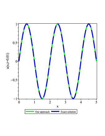
(a) Exact and approximate solution at $\alpha=1$

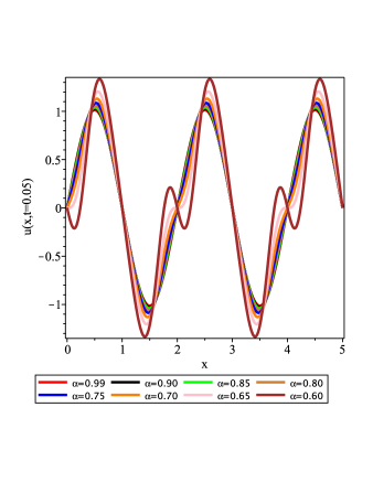
(b) Solution plot for different $\alpha$

Figure 1: Comparison solution plots up to three terms approximation for Problem 1.

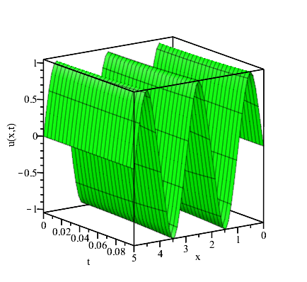
(a) 3D approximate solution

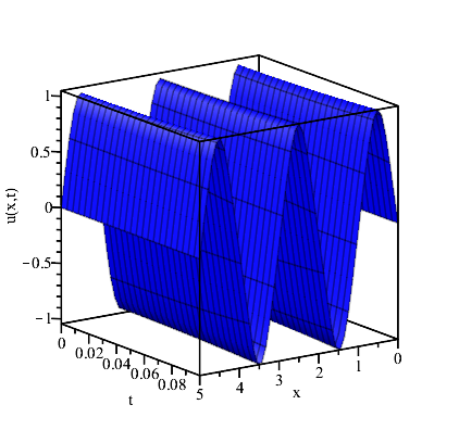
(b) 3D exact solution

Figure 2: Comparison solution plots up to three terms approximation for Problem 1 at $\alpha=1$.

Problem 2.

Next, we consider the FPIDE (4.1) with source term $f(x,t)$

$$\begin{split}f({{{{x}}}},{{{{t}}}})&=\left(6\,{\frac{{t}^{3-\alpha}}{\Gamma\left(4-\alpha\right)}}+\pi\,{t}^{6}\cos\left(\pi\,x\right)+6\,{\frac{{\pi}^{2}\Gamma\left(\alpha\right){t}^{3+\alpha}}{\Gamma\left(4+\alpha\right)}}\right)\sin\left(\pi\,x\right)\end{split}$$ (4.5)

and initial condition $u(x,0)$

$${{{{u}}}}({{{{x}}}},0)=0.$$ (4.6)

The exact solution to equations (4.1), (4.5) and (4.6) is

$${{{{u}}}}({{{{x}}}},{{{{t}}}})={t}^{3}\sin\left(\pi\,x\right).$$

Table 2 shows the numerical simulations for the approximate solution and the exact solution respectively for Problem 2. Figure 3 shows the comparison solution plots for Problem 2 for various values of $\alpha$, and Figure 4 shows the comparison plots between approximate solution and exact solution at $\alpha=1$.

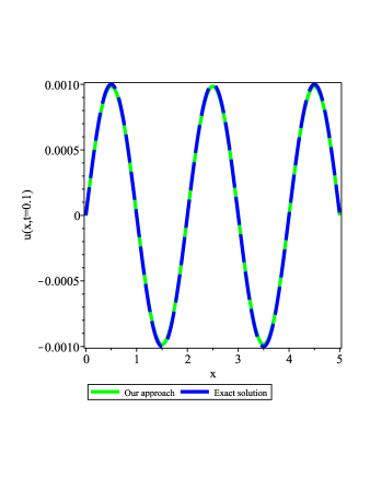
(a) Exact and approximate solution at $\alpha=1$

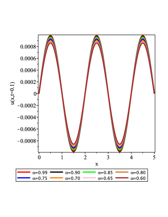
(b) Solution plot for different $\alpha$

Figure 3: Comparison solution plots up to three terms approximation for Problem 2.

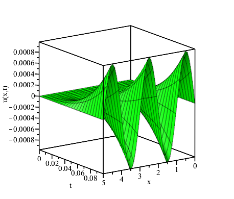
(a) 3D approximate solution

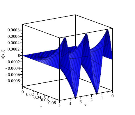
(b) 3D exact solution

Figure 4: Comparison solution plots up to three terms approximation for Problem 2 at $\alpha=1$.

Table 2: Numerical simulations across various iterations, time levels, and spatial domains for the Problem 2 at $\alpha=1$.

${{{t}}}$	${{x}}$	Approximate solution	Exact solution	Absolute error at 1st iteration	Absolute error at 2nd iteration	Absolute error at 3rd iteration
$0.01$	$0.1$	$0.000\,000\,309$	$0.000\,000\,309$	$6.10\text{\times}{10}^{-11}$	$8.60\text{\times}{10}^{-15}$	$9.44\text{\times}{10}^{-19}$
$0.01$	$0.3$	$0.000\,000\,809$	$0.000\,000\,809$	$1.60\text{\times}{10}^{-10}$	$2.25\text{\times}{10}^{-14}$	$2.47\text{\times}{10}^{-18}$
$0.01$	$0.5$	$0.000\,001\,000$	$0.000\,001\,000$	$1.97\text{\times}{10}^{-10}$	$2.78\text{\times}{10}^{-14}$	$3.05\text{\times}{10}^{-18}$
$0.01$	$0.7$	$0.000\,000\,809$	$0.000\,000\,809$	$1.60\text{\times}{10}^{-10}$	$2.25\text{\times}{10}^{-14}$	$2.47\text{\times}{10}^{-18}$
$0.01$	$0.9$	$0.000\,000\,309$	$0.000\,000\,309$	$6.10\text{\times}{10}^{-11}$	$8.60\text{\times}{10}^{-15}$	$9.43\text{\times}{10}^{-19}$
$0.03$	$0.1$	$0.000\,008\,343$	$0.000\,008\,343$	$1.48\text{\times}{10}^{-08}$	$1.88\text{\times}{10}^{-11}$	$1.86\text{\times}{10}^{-14}$
$0.03$	$0.3$	$0.000\,021\,843$	$0.000\,021\,843$	$3.88\text{\times}{10}^{-08}$	$4.93\text{\times}{10}^{-11}$	$4.87\text{\times}{10}^{-14}$
$0.03$	$0.5$	$0.000\,027\,000$	$0.000\,027\,000$	$4.80\text{\times}{10}^{-08}$	$6.09\text{\times}{10}^{-11}$	$6.01\text{\times}{10}^{-14}$
$0.03$	$0.7$	$0.000\,021\,843$	$0.000\,021\,843$	$3.88\text{\times}{10}^{-08}$	$4.92\text{\times}{10}^{-11}$	$4.85\text{\times}{10}^{-14}$
$0.03$	$0.9$	$0.000\,008\,343$	$0.000\,008\,343$	$1.48\text{\times}{10}^{-08}$	$1.88\text{\times}{10}^{-11}$	$1.85\text{\times}{10}^{-14}$
$0.05$	$0.1$	$0.000\,038\,627$	$0.000\,038\,627$	$1.91\text{\times}{10}^{-07}$	$6.74\text{\times}{10}^{-10}$	$1.86\text{\times}{10}^{-12}$
$0.05$	$0.3$	$0.000\,101\,127$	$0.000\,101\,127$	$4.99\text{\times}{10}^{-07}$	$1.76\text{\times}{10}^{-09}$	$4.85\text{\times}{10}^{-12}$
$0.05$	$0.5$	$0.000\,125\,000$	$0.000\,125\,000$	$6.17\text{\times}{10}^{-07}$	$2.17\text{\times}{10}^{-09}$	$5.96\text{\times}{10}^{-12}$
$0.05$	$0.7$	$0.000\,101\,127$	$0.000\,101\,127$	$4.99\text{\times}{10}^{-07}$	$1.76\text{\times}{10}^{-09}$	$4.79\text{\times}{10}^{-12}$
$0.05$	$0.9$	$0.000\,038\,627$	$0.000\,038\,627$	$1.91\text{\times}{10}^{-07}$	$6.70\text{\times}{10}^{-10}$	$1.82\text{\times}{10}^{-12}$
$0.07$	$0.1$	$0.000\,105\,993$	$0.000\,105\,993$	$1.03\text{\times}{10}^{-06}$	$7.12\text{\times}{10}^{-09}$	$3.89\text{\times}{10}^{-11}$
$0.07$	$0.3$	$0.000\,277\,493$	$0.000\,277\,493$	$2.69\text{\times}{10}^{-06}$	$1.86\text{\times}{10}^{-08}$	$1.01\text{\times}{10}^{-10}$
$0.07$	$0.5$	$0.000\,343\,000$	$0.000\,343\,000$	$3.32\text{\times}{10}^{-06}$	$2.29\text{\times}{10}^{-08}$	$1.23\text{\times}{10}^{-10}$
$0.07$	$0.7$	$0.000\,277\,493$	$0.000\,277\,493$	$2.68\text{\times}{10}^{-06}$	$1.85\text{\times}{10}^{-08}$	$9.84\text{\times}{10}^{-11}$
$0.07$	$0.9$	$0.000\,105\,993$	$0.000\,105\,993$	$1.02\text{\times}{10}^{-06}$	$7.04\text{\times}{10}^{-09}$	$3.73\text{\times}{10}^{-11}$
$0.09$	$0.1$	$0.000\,225\,274$	$0.000\,225\,273$	$3.61\text{\times}{10}^{-06}$	$4.15\text{\times}{10}^{-08}$	$3.78\text{\times}{10}^{-10}$
$0.09$	$0.3$	$0.000\,589\,774$	$0.000\,589\,773$	$9.44\text{\times}{10}^{-06}$	$1.08\text{\times}{10}^{-07}$	$9.77\text{\times}{10}^{-10}$
$0.09$	$0.5$	$0.000\,729\,001$	$0.000\,729\,000$	$1.17\text{\times}{10}^{-05}$	$1.33\text{\times}{10}^{-07}$	$1.18\text{\times}{10}^{-09}$
$0.09$	$0.7$	$0.000\,589\,774$	$0.000\,589\,773$	$9.42\text{\times}{10}^{-06}$	$1.07\text{\times}{10}^{-07}$	$9.36\text{\times}{10}^{-10}$
$0.09$	$0.9$	$0.000\,225\,274$	$0.000\,225\,273$	$3.60\text{\times}{10}^{-06}$	$4.08\text{\times}{10}^{-08}$	$3.53\text{\times}{10}^{-10}$

Problem 3.

Finally, we consider the FPIDE (4.1) with source term $f(x,t)$

$$\begin{split}f({{{{x}}}},{{{{t}}}})&={\frac{\Gamma\left(7/2\right){{{{{t}}}}}^{5/2-{{{{\alpha}}}}}{{{{{x}}}}}^{2}\left(1-{{{{{x}}}}}\right)^{2}}{\Gamma\left(7/2-{{{{\alpha}}}}\right)}}-2\,\left({\frac{{{{{{t}}}}}^{{{{{\alpha}}}}}}{{{{{\alpha}}}}}}+\,{\frac{\Gamma\left(7/2\right)\Gamma\left({{{{\alpha}}}}\right){{{{{t}}}}}^{5/2+{{{{\alpha}}}}}}{\Gamma\left(7/2+{{{{\alpha}}}}\right)}}\right)\left(6\,{{{{{x}}}}}^{2}-6\,{{{{{x}}}}}+1\right)\\ &+2\,\left(1+{{{{{t}}}}}^{5/2}\right)^{2}\left(1-2\,{{{{{x}}}}}\right){{{{{x}}}}}^{3}\left(1-{{{{{x}}}}}\right)^{3}\end{split}$$ (4.7)

and initial condition $u(x,0)$

$${{{{u}}}}({{{{x}}}},0)={{{{{x}}}}}^{2}\left(1-{{{{{x}}}}}\right)^{2}.$$ (4.8)

The exact solution solution to equations (4.1), (4.7) and (4.8) is

$${{{{u}}}}({{{{x}}}},{{{{t}}}})=\left(1+{{{{{t}}}}}^{5/2}\right){{{{{x}}}}}^{2}\left(1-{{{{{x}}}}}\right)^{2}.$$

Table 3 shows the numerical simulations for the approximate solution and the exact solution respectively for Problem 3. Figure 5 shows the comparison solution plots for Problem 3 for various values of $\alpha$, and Figure 6 shows the comparison plots between approximate solution and exact solution at $\alpha=1$.

Table 3: Numerical simulations across various iterations, time levels, and spatial domains for the Problem 3 at $\alpha=1$.

${{{t}}}$	${{x}}$	Approximate solution	Exact solution	Absolute error at 1st iteration	Absolute error at 2nd iteration	Absolute error at 3rd iteration
$0.001$	$0.2$	$0.025\,600\,001$	$0.025\,600\,001$	$1.05\text{\times}{10}^{-09}$	$1.59\text{\times}{10}^{-13}$	$1.95\text{\times}{10}^{-17}$
$0.001$	$0.4$	$0.057\,600\,002$	$0.057\,600\,002$	$7.58\text{\times}{10}^{-10}$	$3.98\text{\times}{10}^{-13}$	$2.93\text{\times}{10}^{-17}$
$0.001$	$0.6$	$0.057\,600\,002$	$0.057\,600\,002$	$1.09\text{\times}{10}^{-09}$	$3.35\text{\times}{10}^{-13}$	$2.50\text{\times}{10}^{-17}$
$0.001$	$0.8$	$0.025\,600\,001$	$0.025\,600\,001$	$8.99\text{\times}{10}^{-10}$	$6.89\text{\times}{10}^{-14}$	$8.29\text{\times}{10}^{-18}$
$0.001$	$1.0$	$-0.000\,000\,000$	$0.000\,000\,000$	$3.00\text{\times}{10}^{-12}$	$1.92\text{\times}{10}^{-14}$	$6.05\text{\times}{10}^{-18}$
$0.003$	$0.2$	$0.025\,600\,013$	$0.025\,600\,013$	$1.10\text{\times}{10}^{-08}$	$7.10\text{\times}{10}^{-12}$	$4.95\text{\times}{10}^{-15}$
$0.003$	$0.4$	$0.057\,600\,028$	$0.057\,600\,028$	$3.59\text{\times}{10}^{-09}$	$1.19\text{\times}{10}^{-11}$	$7.24\text{\times}{10}^{-15}$
$0.003$	$0.6$	$0.057\,600\,028$	$0.057\,600\,028$	$1.26\text{\times}{10}^{-08}$	$6.77\text{\times}{10}^{-12}$	$5.88\text{\times}{10}^{-15}$
$0.003$	$0.8$	$0.025\,600\,013$	$0.025\,600\,013$	$6.97\text{\times}{10}^{-09}$	$2.22\text{\times}{10}^{-13}$	$2.07\text{\times}{10}^{-15}$
$0.003$	$1.0$	$-0.000\,000\,000$	$0.000\,000\,000$	$2.43\text{\times}{10}^{-10}$	$4.67\text{\times}{10}^{-12}$	$4.24\text{\times}{10}^{-15}$
$0.005$	$0.2$	$0.025\,600\,045$	$0.025\,600\,045$	$3.54\text{\times}{10}^{-08}$	$4.75\text{\times}{10}^{-11}$	$7.51\text{\times}{10}^{-14}$
$0.005$	$0.4$	$0.057\,600\,102$	$0.057\,600\,102$	$4.00\text{\times}{10}^{-10}$	$5.72\text{\times}{10}^{-11}$	$9.63\text{\times}{10}^{-14}$
$0.005$	$0.6$	$0.057\,600\,102$	$0.057\,600\,102$	$4.23\text{\times}{10}^{-08}$	$1.80\text{\times}{10}^{-11}$	$7.01\text{\times}{10}^{-14}$
$0.005$	$0.8$	$0.025\,600\,045$	$0.025\,600\,045$	$1.68\text{\times}{10}^{-08}$	$9.02\text{\times}{10}^{-12}$	$2.24\text{\times}{10}^{-14}$
$0.005$	$1.0$	$-0.000\,000\,000$	$0.000\,000\,000$	$1.88\text{\times}{10}^{-09}$	$6.00\text{\times}{10}^{-11}$	$8.71\text{\times}{10}^{-14}$
$0.007$	$0.2$	$0.025\,600\,105$	$0.025\,600\,105$	$8.02\text{\times}{10}^{-08}$	$1.75\text{\times}{10}^{-10}$	$4.79\text{\times}{10}^{-13}$
$0.007$	$0.4$	$0.057\,600\,236$	$0.057\,600\,236$	$1.92\text{\times}{10}^{-08}$	$1.56\text{\times}{10}^{-10}$	$5.34\text{\times}{10}^{-13}$
$0.007$	$0.6$	$0.057\,600\,236$	$0.057\,600\,236$	$9.58\text{\times}{10}^{-08}$	$5.31\text{\times}{10}^{-12}$	$3.43\text{\times}{10}^{-13}$
$0.007$	$0.8$	$0.025\,600\,105$	$0.025\,600\,105$	$2.93\text{\times}{10}^{-08}$	$4.21\text{\times}{10}^{-11}$	$1.02\text{\times}{10}^{-13}$
$0.007$	$1.0$	$-0.000\,000\,000$	$0.000\,000\,000$	$7.22\text{\times}{10}^{-09}$	$3.23\text{\times}{10}^{-10}$	$6.28\text{\times}{10}^{-13}$
$0.009$	$0.2$	$0.025\,600\,197$	$0.025\,600\,197$	$1.52\text{\times}{10}^{-07}$	$4.76\text{\times}{10}^{-10}$	$1.99\text{\times}{10}^{-12}$
$0.009$	$0.4$	$0.057\,600\,443$	$0.057\,600\,443$	$6.66\text{\times}{10}^{-08}$	$3.13\text{\times}{10}^{-10}$	$1.92\text{\times}{10}^{-12}$
$0.009$	$0.6$	$0.057\,600\,443$	$0.057\,600\,443$	$1.78\text{\times}{10}^{-07}$	$9.84\text{\times}{10}^{-11}$	$1.07\text{\times}{10}^{-12}$
$0.009$	$0.8$	$0.025\,600\,197$	$0.025\,600\,197$	$4.41\text{\times}{10}^{-08}$	$1.17\text{\times}{10}^{-10}$	$3.19\text{\times}{10}^{-13}$
$0.009$	$1.0$	$-0.000\,000\,000$	$0.000\,000\,000$	$1.98\text{\times}{10}^{-08}$	$1.13\text{\times}{10}^{-09}$	$2.71\text{\times}{10}^{-12}$

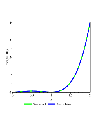
(a) Exact and approximate solution

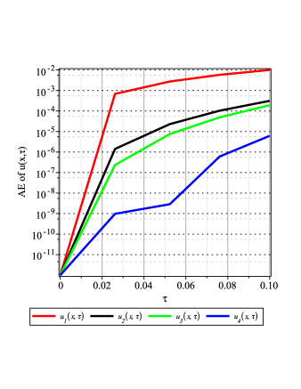
(b) Error for different iterations

Figure 5: Comparison solution plots up to three terms approximation for Problem 3.

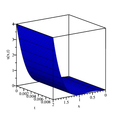
(a) 3D approximate solution

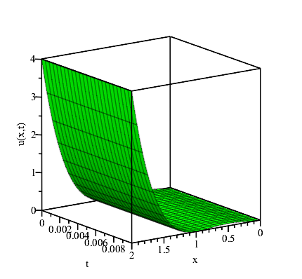
(b) 3D exact solution

Figure 6: Comparison solution plots up to three terms approximation for Problem 3 at $\alpha=1$.

5 Results and Discussions

In this section, we discuss the results as obtained in Section 4. We observe that the non-linearity is directly handled by using a broader concept of the Daftardar–Jafari polynomials. The numerical simulation is conducted in the following steps:

• The Aboodh transform (AT) is applied to the fractional derivative in the Laplace domain to obtain a simpler algebraic form of the problem.

• The iterative procedure is considered with Daftardar–Jafari polynomials to obtain the numerical results.

• The inverse of AT is implemented to get back to the $time$ domain from the $s$ domain.

We claim that our new scheme IATM has a higher accuracy than LADM, which can be established through numerical simulation as provided in Section 4. In fact, the claimed higher accuracy is not due to the Aboodh transformation. By utilizing Daftardar–Jafari polynomials $\mathbf{J}_{j}$ for the non-linear term given in (4.2), $\mathbf{J}_{j}$ can work more effectively as compared to Adomian polynomials $\mathbf{P}_{j}$. More precisely, as we have seen from the definitions of $\mathbf{J}_{j}$ and $\mathbf{P}_{j}$ given in Section 4, it is obvious that the initial iterations of these polynomials are identical. However, starting from the $1^{st}$ iteration, $\mathbf{J}_{1}$ will involve more terms than $\mathbf{P}_{1}$ since more additional terms will start to emerge from $\mathbf{J}_{1}$. Due to those additional terms emerging from the Daftardar–Jafari polynomials, these terms can no doubt help achieve higher accuracy, which contributes to the difference in accuracy between the iterative schemes LADM and IATM.

The beauty of fractional order cannot be underestimated, as it demonstrates a very high convergence rate towards both integer order solutions and the exact solution. We have used different fractional orders and observed that if $\alpha\in(0.5,1]$, then the solutions tend to converge to the exact solution very quickly. These results have been confirmed through subfigures 2(b) and 4(b). We have also found that by using Daftardar–Jafari polynomials, the fractional order solutions converge faster compared to the fractional solutions obtained from Adomian polynomials. Thus, we conclude that IATM works accurately not only for integer order but also for fractional order solutions compared to LADM.

It is clear that Daftardar–Jafari polynomials require more computational resources compared to Adomian polynomials, but we are grateful to the STEM Lab of the Education University of Hong Kong for facilitating us with a GPU system powered by an Intel(R) Core(TM) i9-8950HK. All the experiments and plots have been conducted using Maple Version 2024 in the STEM Lab. The graphical representation confirms the effectiveness of the proposed method, where we compared the exact solution with our obtained approximate solution. We also observe that as we add more terms to the series solution $u(x,t)$, the accuracy of the methods increases gradually. It has been confirmed by the absolute error for different numbers of iterations.

6 Conclusion and Future Work

In summary, we introduce a new method known as Iterative Aboodh transform method (IATM) in which the non-linear terms in the FPIDEs are expressed in terms of Daftardar–Jafari polynomials. The present procedure required a small number of calculations to achieve the higher accurate solutions of the targeted problems. The approximate solutions are expressed in series form of the proposed polynomials and they are illustrated with graphs and tables. It is observed that the suggested method has applicability towards both fractional and integer order problems. Furthermore, we find that fractional solutions gradually converge to solutions with integral order of derivative as $\alpha\to 1$. The present approach is simple to be implemented for non-linear problems, which makes it suitable for studying other non-linear FPIDEs and related systems. One possible extension could be the non-linear stochastic fractional integro-differential equations with suitable initial conditions. The non-linear term can be controlled by Daftardar–Jafari polynomials, and the fractional derivative can be simplified using Laplace or Abooth transformations. However, one needs to be more careful about how to control the stochastic terms in each iteration, which could be one of our possible future directions for research.

CRediT authorship contribution statement

Qasim Khan: Methodology, Conceptualization, Investigation, Software, Data curation, Validation, Visualization, Resources, Formal analysis, & Writing – original draft.
Anthony Suen: Supervision, Investigation, Project administration, Funding, Writing – review & editing.

Declaration of competing interest

The authors declare that they have no known competing financial interests or personal relationships that could have appeared to influence the work reported in this research paper.

Data availability

No data was used for the research described in the article.

Funding

This work is partially supported by Hong Kong General Research Fund (GRF) grant project number 18300821, 18300622 and 18300424, and the EdUHK Research Incentive Award project titled “Analytic and numerical aspects of partial differential equations”.

Acknowledgment

We are very grateful to our MIT lab mates and the technicians at STEM lab of The Education University of Hong Kong for providing all the necessary facilities for this research work.

References

• [1] F. Mainardi. Fractional Calculus and Waves in Linear Viscoelasticity. Imperial College Press, London, 2010.
• [2] G. M. Zaslavsky. Hamiltonian Chaos and Fractional Dynamics. Oxford University Press, Oxford, UK, 2005.
• [3] I. Podlubny. Fractional Differential Equations. Academic Press, San Diego, CA, USA, 1999.
• [4] A. Kilbas, H. Srivastava, and J. Trujillo. Theory and Applications of Fractional Differential Equations. Elsevier, Amsterdam, The Netherlands, 2006.
• [5] H. Khan and M. Arif. Numerical solutions of some higher order fractional integro-differential equations (fides), using chebyshev wavelet method (cwm). J. Appl. Environ. Biol. Sci., 7(9):105–114, 2017.
• [6] S. T. Mohyud-Din, H. Khan, M. Arif, and M. Rafiq. Chebyshev wavelet method to nonlinear fractional volterra–fredholm integro-differential equations with mixed boundary conditions. Adv. Mech. Eng., 9(3):1687814017694802, 2017.
• [7] A. K. Hussain, N. Rusli, F. S. Fadhel, and Z. R. Yahya. Solution of one-dimensional fractional order partial integro-differential equations using variational iteration method. AIP Conf. Proc., 1775:030096, 2016.
• [8] R. C. Mittal and R. Nigam. Solution of fractional integro-differential equations by adomian decomposition method. Int. J. Appl. Math. Mech., 4:87–94, 2008.
• [9] H. Jaradat, F. Awawdeh, and E.A. Rawashdeh. Analytic solution of fractional integro-differential equations. Ann. Univ. Craiova, 38:1–10, 2011.
• [10] M. R. Eslahchi, M. Dehghan, and M. Parvizi. Application of the collocation method for solving nonlinear fractional integro-differential equations. J. Comput. Appl. Math., 257:105–128, 2014.
• [11] J. Zhao, J. Xiao, and N. J. Ford. Collocation methods for fractional integro-differential equations with weakly singular kernels. Numer. Algorithms, 65:723–743, 2014.
• [12] E. Rawashdeh. Numerical solution of fractional integro-differential equations by collocation method. Appl. Math. Comput., 176:1–6, 2006.
• [13] S. I. Unhale and S. D. Kendre. Numerical solution of nonlinear fractional integro-differential equation by collocation method. Malaya J. Matematik, 6:73–79, 2018.
• [14] Z. Avazzadeh, M. H. Heydari, and C. Cattani. Legendre wavelets for fractional partial integro-differential viscoelastic equations with weakly singular kernels. Eur. Phys. J. Plus, 134:368, 2019.
• [15] S. Arshed. B-spline solution of fractional integro partial differential equation with a weakly singular kernel. Numer. Methods Partial Differential Equations, 33:1565–1581, 2017.
• [16] H. Dehestani, Y. Ordokhani, and M. Razzaghi. Numerical solution of variable-order time fractional weakly singular partial integro-differential equations with error estimation. Math. Model. Anal., 25:680–701, 2020.
• [17] Farshid Mirzaee, Shiva Naserifar, and Erfan Solhi. Meshless barycentric rational interpolation method for solving nonlinear stochastic fractional integro-differential equations. Iranian Journal of Science, 48(3):709–733, 2024.
• [18] Farshid Mirzaee, Erfan Solhi, and Shiva Naserifar. Approximate solution of stochastic volterra integro-differential equations by using moving least squares scheme and spectral collocation method. Applied Mathematics and Computation, 410:126447, 2021.
• [19] Farshid Mirzaee and Sahar Alipour. Bicubic b-spline functions to solve linear two-dimensional weakly singular stochastic integral equation. Iranian Journal of Science and Technology, Transactions A: Science, 45(3):965–972, 2021.
• [20] Farshid Mirzaee and Sahar Alipour. Cubic b-spline approximation for linear stochastic integro-differential equation of fractional order. Journal of Computational and Applied Mathematics, 366:112440, 2020.
• [21] Erfan Solhi, Farshid Mirzaee, and Shiva Naserifar. Enhanced moving least squares method for solving the stochastic fractional volterra integro-differential equations of hammerstein type. Numerical Algorithms, 95(4):1921–1951, 2024.
• [22] Sahar Alipour and Farshid Mirzaee. An iterative algorithm for solving two dimensional nonlinear stochastic integral equations: A combined successive approximations method with bilinear spline interpolation. Applied Mathematics and Computation, 371:124947, 2020.
• [23] Farshid Mirzaee and Sahar Alipour. Numerical solution of nonlinear partial quadratic integro-differential equations of fractional order via hybrid of block-pulse and parabolic functions. Numerical Methods for Partial Differential Equations, 35(3):1134–1151, 2019.
• [24] Nasrin Samadyar and Farshid Mirzaee. Numerical scheme for solving singular fractional partial integro-differential equation via orthonormal bernoulli polynomials. International Journal of Numerical Modelling: Electronic Networks, Devices and Fields, 32(6):e2652, 2019.
• [25] V. Daftardar-Gejji and H. Jafari. An iterative method for solving nonlinear functional equations. J. Math. Anal. Appl., 316(2):753–763, 2006.
• [26] Q. Khan and A. Suen. Comparative analysis of polynomials with their computational costs. arXiv preprint arXiv:2411.00487, 2024.
• [27] Q. Khan, H. Khan, P. Kumam, F. Tchier, and G. Singh. Ladm procedure to find the analytical solutions of the nonlinear fractional dynamics of partial integro-differential equations. Demonstratio Math., 57:20230101, 2024.
• [28] J. Guo, D. Xu, and W. Qiu. A finite difference scheme for the nonlinear time-fractional partial integro-differential equation. Math. Methods Appl. Sci., 43:1–21, 2020.
• [29] M. Caputo. Elasticità e Dissipazione. Zanichelli, Bologna, 1969.
• [30] M. Caputo. Linear model of dissipation whose q is almost frequency independent-ii. Geophys. J. R. Astron. Soc., 13:529–539, 1967.
• [31] M. G. Mittag-Leffler. Sur la nouvelle fonction. Comptes Rendus Acad. Sci. Paris, 137:554–558, 1903.
• [32] K. S. Aboodh. The new integral transform ”aboodh transform”. Global J. Pure Appl. Math., 9(1):35–43, 2013.
• [33] K. S. Aboodh. Application of new transform ”aboodh transform” to partial differential equations. Global J. Pure Appl. Math., 10(2):249–254, 2014.
• [34] T. G. Thange and A. R. Gade. On aboodh transform for fractional differential operator. Malaya J. Matematik (MJM), 8(1):225–229, 2020.
• [35] Q. Khan, A. Suen, and H. Khan. Application of an efficient analytical technique based on aboodh transformation to solve linear and non-linear dynamical systems of integro-differential equations. Part. Differ. Equ. Appl. Math., 11:100848, 2024.
• [36] Q. Khan, A. Suen, H. Khan, and P. Kumam. Comparative analysis of fractional dynamical systems with various operators. AIMS Math., 8(6):13943–13983, 2023.
• [37] Qasim Khan. An efficient approach to fractional analysis for non-linear coupled thermo-elastic systems. arXiv preprint arXiv:2501.06127, 2025.
• [38] Mukesh Kumar Rawani, Amit Kumar Verma, and Carlo Cattani. A novel hybrid approach for computing numerical solution of the time-fractional nonlinear one and two-dimensional partial integro-differential equation. Communications in Nonlinear Science and Numerical Simulation, 118:106986, 2023.
• [39] T. Akram, Z. Ali, F. Rabiei, K. Shah, and P. Kumam. A numerical study of nonlinear fractional order partial integro-differential equation with a weakly singular kernel. Fractals Fract., 5(3):85, 2021.