Hyperspherical Energy Transformer with Recurrent Depth

Abstract

Transformer-based foundation models have achieved unprecedented success with a gigantic amount of parameters and computational resources. Yet, the core building blocks of these models, the Transformer layers, and how they are arranged and configured are primarily engineered from the bottom up and driven by heuristics. For advancing next-generation architectures, it demands exploring a prototypical model that is amenable to high interpretability and of practical competence. To this end, we take a step from the top-down view and design neural networks from an energy minimization perspective. Specifically, to promote isotropic token distribution on the sphere, we formulate a modified Hopfield energy function on the subspace-embedded hypersphere, based on which Transformer layers with symmetric structures are designed as the iterative optimization for the energy function. By integrating layers with the same parameters, we propose Hyper-Spherical Energy Transformer (Hyper-SET), an alternative to the vanilla Transformer with recurrent depth. This design inherently provides greater interpretability and allows for scaling to deeper layers without a significant increase in the number of parameters. We also empirically demonstrate that Hyper-SET achieves comparable or even superior performance on both synthetic and real-world tasks, such as solving Sudoku and masked image modeling, while utilizing fewer parameters.

1 Introduction

Transformer-based models (Vaswani et al., 2017) have become foundational across diverse domains across diverse domains, including computer vision (Dosovitskiy et al., 2021; Bao et al., 2022; He et al., 2022; Peebles & Xie, 2023), natural language processing (Devlin et al., 2019; Lan et al., 2020; Brown et al., 2020), robotics (Brohan et al., 2022), decision-making (Chen et al., 2021), scientific discovery (Jumper et al., 2021; Kamienny et al., 2022), and so on. In recent years, there has been evidence that scaling up model size, dataset size or computational budget to a gigantic magnitude during pre-training can bring about unprecedented performance gains (Kaplan et al., 2020), driving the proliferation of Transformer-based foundation models (OpenAI et al., 2024; Dubey et al., 2024; Anil et al., 2023; Oquab et al., 2024).

On the other hand, despite the remarkable abilities of Transformer-based Large Language Models (LLMs), the design and modifications of the Transformer architectures are largely driven by experience and heuristics. There is limited principled guidance for the model’s configuration, e.g., how many layers should be stacked. In fact, some empirical studies have observed high redundancy in the deeper layers (Gromov et al., 2024; Men et al., 2024), uniformity of representations in the middle layers (Sun et al., 2024), and robustness to swapping certain intermediate layers (Lad et al., 2024) in LLMs. This suggests convergent functionality one layer represents, yet we have a limited understanding of what role the layer plays in processing information and representation learning. Although there are efforts to unveil the function or algorithms underlying the network layers, especially Transformer blocks, through mechanistic interpretability (Elhage et al., 2021; Nanda et al., 2023; Wang et al., 2023; Conmy et al., 2023; Huben et al., 2024), causal mediation analysis (Vig et al., 2020; Meng et al., 2022), visualization (Bricken et al., 2023; Olsson et al., 2022), and others, most of them focus on post hoc interpretation and phenomenological approaches. A natural question arises: Can we find or design a function prior that induces a model that is interpretable by construction?

One way is to incorporate explicitly optimization process or problem-solving into the neural architecture via model-based deep learning (Shlezinger et al., 2023), such as solving constraint satisfiability problems (Wang et al., 2019), optimal control (Amos & Kolter, 2017; Amos et al., 2018), inverse problems (Scarlett et al., 2022), physical law (Greydanus et al., 2019; Karniadakis et al., 2021; Thuerey et al., 2021), etc. Despite its success, it is mostly limited to domain-specific priors. Another line of work revolves around a unified view of learning, optimization, and model architectures through the energy-based learning framework (Dawid & LeCun, 2024), where it casts modeling the relation or constraint between input $x$ and output $y$ as a scalar-valued energy function $E_{\theta}(x,y)$ and the inference as finding the minimizer of the function given the input $\hat{y}=\text{min}_{y}E_{\theta}(x,y)$. Drawing on this view, a number of articles have considered layers as optimization of a generic energy function, either defined implicitly (Bai et al., 2019; Du et al., 2022) by a neural network or explicitly with inspiration from other fields (Hoover et al., 2024; Yu et al., 2023). A single iteration of energy optimization is usually viewed as one-layer update of the given input, which reveals the dynamics of the function. In particular, Hopfield energy has been recently revived to establish connections to Transformers in terms of content-addressable associative memory (Ramsauer et al., 2021; Bricken & Pehlevan, 2021; Krotov, 2023; Bietti et al., 2023), where the attention module is interpreted as an information retrieval system that navigates input to the energy stationary points.

In this paper, we contribute to understanding Transformer-based models from the energy learning perspective. We adopt deep unrolling that unfolds the optimization of an objective function via, e.g., gradient descent to establish equivalence to the network layer. Concretely, we consider tokens as particles and model their dynamics on the hypersphere inspired by (Sander et al., 2022; Geshkovski et al., 2023a, b). We define a dual Hopfield energy function, where one promotes tokens to distribute isotopically in subspaces to mitigate the synchronization effect while the other enforces directional alignment with bases of the original space. By minimizing them alternatively, we derive the core components in Transformers: skip connection, $\operatorname{RMSNorm(\cdot)}$, and a new self-attention and feedforward module with symmetric structures. Each component has its own precise functionality, thus interpretable by design. We name this model Hyper-Spherical Energy Transformer (Hyper-SET). By comparing it with vanilla Transformers on both synthetic and real-world tasks, we demonstrate its competitive, even better, performance while being parameter-efficient. The key contributions are summarized as follows

1. Theoretical Formulation: Motivated by Hopfield energy, we introduce a unified hyperspherical energy function and provide their theoretical insights.

2. Energy-Driven Architecture: We build a Transformer-based model with parameter efficiency from sheer energy minimization.

3. Competitive Performance: We show its competitive performance to vanilla Transformers across reasoning, classification, and masked image modeling.

2 Related Work

2.1 Energy-based Learning

Energy-based learning (EBL) has been a powerful framework for probabilistic modeling, offering a flexible approach to modeling complex data distributions through the lens of energy functions. The primitive ideas in this vein can date back to the Hopfield network (Hopfield, 1982) and Boltzmann machine (Ackley et al., 1985) and were greatly developed in (LeCun et al., 2006).

A large body of work has revolved around utilizing energy-based models for generative modeling by learning the energy function (Du & Mordatch, 2019) or its gradient, also known as score-based models (Sohl-Dickstein et al., 2015; Song & Ermon, 2019; Song et al., 2021). This approach attempts to model the data distribution represented by an energy function and learns to generate new samples via Langevin dynamics. Another group of work understands EBL as the computation of the network layer (Amos & Kolter, 2017; Agrawal et al., 2019). They consider the layer parallels a domain-specific optimization problem but cannot explicitly define a generic form of the energy function. In this paper, we explicitly define the energy function on the hypersphere and relate its optimization to Transformer layers. There are also similar efforts to learning energy on the hypersphere (Liu et al., 2018; Loshchilov et al., 2024), but our energy functions are different and defined on the representation space instead of weight space.

2.2 Model Design from First Principle

While the architecture of widely used neural networks is often driven by engineering practices, there has been a series of work that seeks to design or interpret neural networks from principled perspectives such as signal processing, information theory, neurobiology, etc. For example, deep unrolling of the sparse coding algorithms has led to the development of fully connected networks (Gregor & LeCun, 2010), convolution networks (Papyan et al., 2017, 2018), and even graph neural networks through iterative algorithms (Yang et al., 2021). Similarly, the sparse rate reduction principle has been used to derive the Transformer architecture (Yu et al., 2023). Other approaches draw inspiration from approximation theory (Liu et al., 2024) and brain computation (Kozachkov et al., 2023), further bridging the gap between theoretical insights and practical network design.

3 Preliminaries

3.1 Hopfield Networks

Given a network with $N$ neurons $\bm{x}=[x_{1},\dots,x_{N}]$ that take binary values, the temporal evolution dynamics of these neurons are determined by a scalar-value energy function

$$E=-\frac{1}{2}\sum_{i,j}\omega_{ij}x_{i}x_{j}=-\frac{1}{2}\bm{x}^{T}\bm{W}\bm{x},\quad x_{i},x_{j}\in\{+1,-1\}$$

where $\omega_{ij}$ represents the strength of connectivity between node $x_{i}$ and $x_{j}$, and connectivity is assumed to be symmetric, i.e., $\omega_{ij}=\omega_{ji}$. We can further rewrite $\bm{W}=\sum_{i=1}^{P}\bm{\xi}_{i}\bm{\xi}_{i}^{T}$ as a set of patterns to be stored. The update rule of each node to retrieve the most relevant pattern follows the Hebbian learning rule used in neuroscience

$$\bm{x}_{t+1}=\text{sign}(\bm{W}\bm{x}_{t})=\text{sign}\left(\sum_{i=1}^{P}\bm{\xi}_{i}\bm{\xi}_{i}^{T}\bm{x}_{t}\right).$$

This update rule tends to minimize the energy function with retrieved patterns as its attractor. It is an embodiment of the idea of “Neurons that fire together wire together.”: If two neurons connect ($\omega_{ij}>0$), then they should have the same state ($+1$ for active and $-1$ for dead). The number of patterns the network can store and retrieve is $\mathcal{O}(N)$.

3.2 Modern Continuous Hopfield Networks

To overcome the limitation of linear storage capacity, modern Hopfield networks, also known as Dense Associative Memory (Krotov & Hopfield, 2016), introduce nonlinearity in the energy and the update of neurons’ states and make them suitable for continuous variables.

$$E=-\frac{1}{2}\sum_{i=1}^{P}f\left(\bm{\xi}_{i}^{T}\bm{x}\right),\ \bm{x}_{t+1}=\operatorname{tanh}\left(\sum_{i=1}^{P}\bm{\xi}_{i}f^{\prime}\left(\bm{\xi}_{i}^{T}\bm{x}_{t}\right)\right),$$

where $\operatorname{tanh(\cdot)}$ is to ensure the neurons’ states are constrained to the interval $[-1,1]$ so that the energy is bounded from below. Depending on the form of $f$, the network could have power or exponential storage capacity. If we set $f(x)=x^{2}$, this reduces to the traditional networks with linear capacity.

If we further make modifications to the non-linearity in the energy function with $\operatorname{logsumexp(\cdot)}$, which is inspired by contrastive normalization, we can define the Modern Continuous Hopfield (MCH) energy function with a quadratic regularization term on $\bm{x}$:

$$E_{\text{MCH}}=-\log\left(\sum_{i=1}^{P}\exp\left(\bm{\xi_{i}}^{T}\bm{x}\right)\right)+\frac{1}{2}\bm{x}^{T}\bm{x}.$$

By leveraging the concave-convex procedure (Yuille & Rangarajan, 2003), the update could be written as

$$\bm{x}_{t+1}=\Xi\operatorname{softmax}(\Xi^{T}\bm{x}_{t}),$$

where $\Xi=[\xi_{1},\dots,\xi_{P}]\in\mathbb{R}^{N\times P}$. This formulation has proven to converge to stationary points of the energy function $E_{\text{MCH}}$, and is linked to the key-value memory similar to the attention mechanism (Ramsauer et al., 2021). Notice that this update rule is essentially the cross-attention given a query vector $\bm{x}$ and can only describe the independent evolution of that vector. It fails to faithfully cover the parallel interactions between contextual tokens in the self-attention adopted in the GPT or BERT style Transformers.

The construction of the modern continuous Hopfield energy and update rule can also be carried out from a biologically plausible view by extending the network with hidden neurons and establishing a group of coupled differential equations. We refer the readers to (Krotov & Hopfield, 2021; Krotov, 2023) for more details.

4 Hypersphere Energy Transformer from Iterative Energy Minimization

In this section, we formulate a new form of energy function as the sum of two modified Hopfield energy functions defined on a hypersphere embedded in multiple subspaces. We will demonstrate how we can derive the structure of Transformers, with self-attention, feedforward, skip connections, and normalization by performing the energy minimization. The overview is presented in Figure 2.

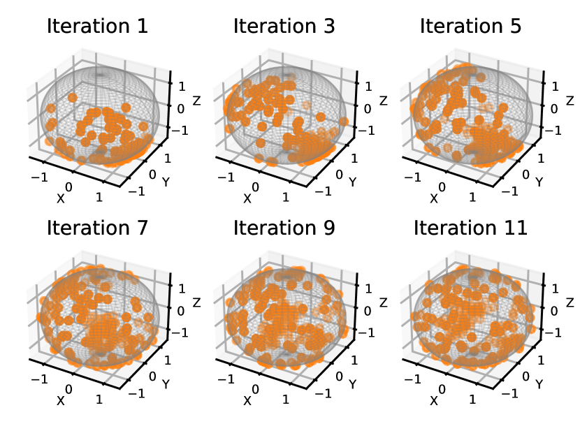
Figure 1: Evolution of Tokens on Subspaces. Tokens projected onto subspaces are progressively separated on the hypersphere as the optimization iterates.

4.1 Hyperspherical Energy

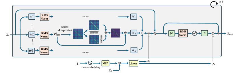
Figure 2: Overview of Our Hyperspherical Energy Transformer Layer. It recovers sequential stacking of symmetric self-attention, feedforward, skip connection and RMSNorm components from sheer minimization of Hopfiel energy. Adaptive step size is learned conditioned the current $t$ and the initial input $\bm{X}_{0}$.

4.1.1 Overcoming Token Synchronization

We consider $N$ vectors $\bm{X}=[\bm{x}_{1},\dots,\bm{x}_{N}]$ from a probabilistic space with $\bm{x}_{i}\in\mathbb{R}^{d},i\in[N]$, which can be seen as the contextual tokens in Transformers, and denote two different sets of basis vectors of this $d$-dimensional space, $\bm{W}=[\bm{W}_{1},\dots,\bm{W}_{H}]\in\mathbb{R}^{d\times Hp}$ and $\bm{D}=[\bm{d}_{1},\dots,\bm{d}_{M}]\in\mathbb{R}^{d\times M}$. Here, $\bm{W}_{i}\in\mathbb{R}^{d\times p}$ represents the projection to the $p$-dimensional subspace. Unless otherwise specified, we assume the column vectors are incoherent and span the full space, i.e., $Hp=M=d$.

A recent study (Yu et al., 2023) argues that the contextual tokens lie on a low-dimensional subspace of its high-dimensional ambient space. We adopt this view and study the projection of tokens with bases $\bm{W}$:

$$\bm{z}_{i}^{h}=\bm{W}_{h}^{T}\bm{x}_{i}.$$ (1)

Minimizing Hopfield energy $E_{\text{MCH}}$ tends to align the vector to the stored patterns while keeping its norm. This interaction occurs between the dynamic tokens and the static stored patterns. However, in Transformers’ self-attention, this interaction happens among all the dynamic tokens simultaneously. Enforcing the tokens to align with one another would make them cluster into one point, losing the expressive power of the module. This phenomenon has been observed in many studies, referred to as token uniformity (Chen et al., 2022; Wu et al., 2024), or rank collapse (Dong et al., 2021), and theoretically characterized in (Geshkovski et al., 2023b). This also relates to the synchronization effect (Acebrón et al., 2005; Miyato et al., 2024).

Therefore, to overcome this issue, we extend the Hopfield energy $E_{\text{MCH}}$ to model the push-away force among tokens. The energy that drives the tokens apart in terms of angles in one subspace would read as

$$E_{\text{ATTN}}^{h}=\beta^{-1}\sum_{i=1}^{N}\log\left(\sum_{j=1}^{N}\exp\left(\beta(\bm{z}_{i}^{h})^{T}(\bm{z}_{j}^{h})\right)\right),$$ (2)

where $\beta$ is usually the inverse of temperature. Here we use the subscript _ATTN as this energy will be shown to be related to the design of the attention layers, resembling that in (Yu et al., 2023). The total energy that models the interacting tokens corresponding to the bases $\bm{W}$ partitioned by different subspaces would be

$$E_{\text{ATTN}}=\sum_{h=1}^{H}E_{\text{ATTN}}^{h},\quad\text{subject to}~\|\bm{W}_{h}^{T}\bm{x}_{i}\|_{2}=\sqrt{p}.$$ (3)

The above dynamics should take place on a hypersphere with its radius determined by the dimension of the subspace. By minimizing (3), the tokens are encouraged to be distributed on the sphere as uniformly as possible. An illustrative example is shown in Figure 1.

4.1.2 Alignment with High-dimensional Bases

The tokens projected to subspaces separate to occupy more volume and enrich the information they encode. To make the overall information minimal and sufficient (Tishby et al., 2000; Tishby & Zaslavsky, 2015), an intuition is that tokens in the original high-dimensional space should encode less information to reduce the uninformative redundancy. This implies that tokens in the original space should coalesce into several distinct clusters. As in high-dimensional space, vectors initialized at random tend to be near-orthogonal (Vershynin, 2018), the basis vectors $\bm{D}$ would naturally comprise these clusters. Thus, it would be reasonable to enable the alignment of tokens with these bases. The energy that implements this idea could be written as

$$E_{\text{FF}} =-\frac{1}{2}\sum_{i=1}^{N}\sum_{m=1}^{M}\left(\operatorname{ReLU}\left(\bm{d}_{m}^{T}\bm{x}_{i}\right)\right)^{2},$$

$$\text{subject to}~\|\bm{D}^{T}\bm{x}_{i}\|_{2}=\sqrt{M}.$$ (4)

Here we use the subscript _FF as this energy will be shown to be related to the design of feedforward layers. By minimizing this energy, a token tends to lie on the union of half-spaces defined by basis vectors that form an acute angle with this token while still residing on the hypersphere of the original space.

4.2 Symmetric Structure Induced From Energy Minimization

By combining the hyperspherical energy defined in Section 4.1, we introduce a unified objective function that characterizes the functionality the Transformer layer represents:

$$\min_{\bm{x}_{1},\dots,\bm{x}_{N}\in\bm{X}}\quad E(\bm{X};\bm{W},\bm{D})=E_{\text{ATTN}}+E_{\text{FF}}$$ (5)

subject to $$\|\bm{W}_{h}^{T}\bm{x}_{i}\|_{2}=\sqrt{p}$$

$$\|\bm{D}^{T}\bm{x}_{i}\|_{2}=\sqrt{M},\quad i=1,\dots,N.$$

This characterization of Transformer optimization problem somewhat resonates with the compression-sparsification procedure in (Yu et al., 2023), where they frame the objective as compressing information of tokens in the subspaces and enlarging volume in the original space. Yet our objective can be interpreted from the opposite direction. We aim to gradually enrich the information in the subspaces while peeling off redundancy in the original space. This also mirrors the rationale of minimal and sufficient statistics from the information bottleneck (Tishby & Zaslavsky, 2015).

To solve optimization (5), we consider an alternating minimization method by splitting it into sub-problems.

4.2.1 Attention Module

To show how we have an attention module derived from minimizing hyperspherical energy, we first establish the differential equation that models the evolution of tokens’ interactions:

$$\begin{split}\dot{\bm{X}}&=-\nabla_{\bm{X}}E_{\text{ATTN}}\\ &=-\sum_{h=1}^{H}\left((\bm{W}_{h}\bm{W}_{h}^{T}\bm{X}\underbrace{\operatorname{softmax}}_{\text{column-wise}}\left(\beta(\bm{W}_{h}^{T}\bm{X})^{T}(\bm{W}_{h}^{T}\bm{X})\right)\right.\\ &\left.\qquad+\bm{W}_{h}\bm{W}_{h}^{T}\bm{X}\underbrace{\operatorname{softmax}}_{\text{row-wise}}\left(\beta(\bm{W}_{h}^{T}\bm{X})^{T}(\bm{W}_{h}^{T}\bm{X})\right)\right)\end{split}$$ (6)

where $\beta=1/\sqrt{p}$ as in standard Transformers (Vaswani et al., 2017). Derivations could be found in Appendix C.1

The constraint on the low-dimensional hypersphere of radius $\sqrt{p}$ corresponds to $\operatorname{RMSNorm(\cdot)}$, which bears resemblance to QK-normalization (Henry et al., 2020), but here the normalization is applied after projection by the same query-key-value matrix. The projection of tokens in $h$-th subspace onto the hypersphere would thus read as

$$\bm{Z}_{\text{RMS}}^{h}=\operatorname{RMSNorm}(\bm{Z}^{h})=\operatorname{RMSNorm}(\bm{W}_{h}^{T}\bm{X}).$$ (7)

By discretizing the differential equation (6) with step size $\alpha_{t}$ and maintaining the hyperspherical constraint with (7), we can derive the complete component that makes up the self-attention module: let $[\bm{Q}\bm{K}]_{\text{RMS,t}}=\beta(\bm{Z}_{\text{RMS},t}^{h})^{T}(\bm{Z}_{\text{RMS},t}^{h})$, then

$$\bm{X}_{t+1} =\bm{X}_{t}-\alpha_{t}\sum_{h=1}^{H}\Bigg{(}\bm{W}_{h}\bm{Z}_{\text{RMS},t}^{h}\underbrace{\operatorname{softmax}}_{\text{column-wise}}\left([\bm{Q}\bm{K}]_{\text{RMS,t}}\right)$$

$$\quad+\bm{W}_{h}\bm{Z}_{\text{RMS},t}^{h}\underbrace{\operatorname{softmax}}_{\text{row-wise}}\left([\bm{Q}\bm{K}]_{\text{RMS,t}}\right)\Bigg{)}.$$ (8)

This update brings up a new attention module with skip connection, and it has highly symmetric structures. On one hand, the query-key dot product is symmetric, while at the same time, the attention matrix is symmetric as well due to the sum of $\operatorname{softmax}$ in both column and row directions. The sum over $H$ different subspaces can be understood as the multi-head structure.

Another interesting connection with prior work is that a doubly stochastic attention matrix has proven to have equivalence to the Wasserstein gradient flow of some global energy (Sander et al., 2022). Here we offer another variant of attention that meets the symmetric query-key dot-production assumption therein and can also be seen as the discretization of an explicit energy function.

4.2.2 FeedForward Module

For the sub-problem of minimizing the other energy, we have a similar construction of the corresponding differential equation, with details deferred to Appendix C.2:

$$\dot{\bm{X}}=-\nabla_{\bm{X}}E_{\text{FF}}=\bm{D}\operatorname{ReLU}\left(\bm{D}^{T}\bm{X}\right).$$ (9)

By further imposing the hypersphercial constraint, we can recover the feedforward layer used in Transformers with step size $\gamma_{t}$:

$$\bm{X}_{t+1}=\bm{X}_{t}+\gamma_{t}\bm{D}\operatorname{ReLU}\left(\operatorname{RMSNorm}\left(\bm{D}^{T}\bm{X}\right)\right)$$ (10)

Notice that this feedforward module also bears symmetry in the weight space.

4.3 Learning Adaptive Step Size

To make the step size more flexible, we choose to learn its embedding with another neural network conditioning on the current iteration $t$ and the initial token $\bm{x}(0)$ (usually the output of the tokenizer):

$$\alpha_{t} =\bm{\alpha}_{\theta}(t,\bm{x}(0)),$$ (11)

$$\gamma_{t} =\bm{\gamma}_{\phi}(t,\bm{x}(0)).$$ (12)

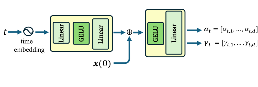
Figure 8: An Illustration of Time Embedding Conditioned on the Input to Learn Adaptive Step size.

For each iteration, step size embeddings in (11) and (12) are applied channel-wise of each token, similar to techniques in (Touvron et al., 2021; Peebles & Xie, 2023) (See Figure 8). We also adopt the zero-initialization of network parameters $\theta$ and $\phi$ from (Bachlechner et al., 2021) to facilitate convergence when using larger iterations.

Combining all the components and techniques, we present the Hyper-Spherical Energy Transformer (Hyper-SET) with attention and feedforward sequentially stacked and with only one layer of learnable parameters. This one-layer model is amenable to rigorous analysis and, as we will demonstrate later, has competitive performance with vanilla Transformer.

5 Experiment

In this section, we compare Hyper-SET with standard Transformers on discriminative and generative learning tasks. For fair comparison, we remove biases in the latter, adopt the Pre-Norm style with $\operatorname{RMSNorm}$, and omit dropout regularization. The MLP ratio in Transformer is set to 4.

As one iteration of energy minimization corresponds to single-layer update of tokens in Hyper-SET, we use one-layer trainable parameters but vary the iteration for all models, including Transformers, unless otherwise specified .

5.1 Solving Sudoku

Solving a Sudoku puzzle involves filling a 9x9 board with partially known digits from 1 to 9, and unknown entries are given as 0. The unknown entries must be filled with digits perfectly such that the board satisfies a certain rule. We tackle this puzzle by predicting the digits to fill in, conditioned on the given digits.

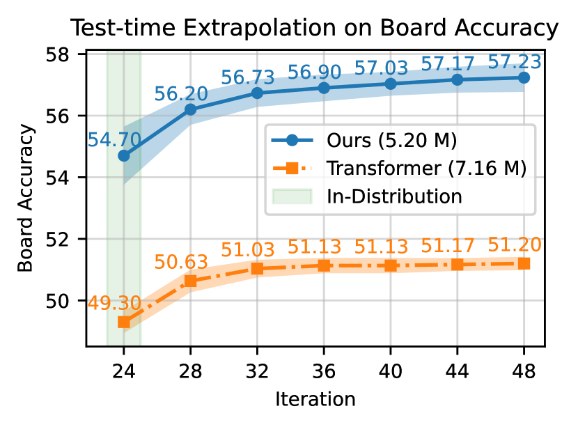
Figure 3: Test-time Extrapolation on Sudoku Board Accuracy w.r.t the Number of Forward Iterations. Our model achieves better performance with fewer parameters, even when the iterations are beyond the training regime. Results are averaged over five runs.

Setup. We adopt the dataset from (Palm et al., 2018) which is considered to be hard, provided that the board thereof only has [17,34] known digits. We build on the code from (Yang et al., 2023) and follow the setting of training on 9k data and evaluating on 1k data. The cross-entropy loss is computed exclusively on the unknown entries.

We train all models for 200 epochs with batch size of 16 and set the optimizer as AdamW (Loshchilov & Hutter, 2019) with 0.1 weight decay. Learning rate is initialized as 1e-4 with cosine decay. The hidden dimension is 768. We measure the accuracy of solving Sudoku on the test dataset. See Appendix A.2 for details.

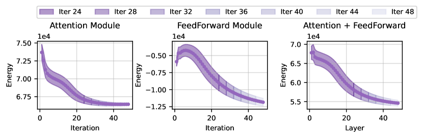
Figure 4: The energy of both the attention and feedforward module decreases on Sudoku (Top) and CIFAR-10 (Bottom), without hard constraints on the sign of the step size. This suggests the layer aligns well with the optimization objective. Normalization is first applied to meet the condition in (5) before computing the energy.

Extrapolation to Larger Iteration. Under the same experimental conditions except for the architectural differences, our model surpasses the standard Transformer for in-distribution iterations (54.70 vs. 49.30), i.e., using the same iterations for both training and inference. The results are displayed in Figure 3.

Solving Sudoku could be seen as a logical reasoning task (Wang et al., 2019). Some efforts have been devoted to allocating more computation at test time for better reasoning and generalization (Schwarzschild et al., 2021; Bansal et al., 2022; Du et al., 2022; Banino et al., 2021), hoping the network can extend the algorithms learned during training.

We build on these views by extending the number of iterations at test time up to two times those during training. As shown in Figure 3, with more computation, our model achieves better scaling behaviors than Transformers with larger improvements on accuracy. This extrapolation could stem from learned adaptive step size that maintains energy minimization trajectory. In practice, we also find out that trainable positional encoding is crucial for the extrapolation.

Energy Evolution. Figure 4 (Top) illustrates the energy trajectory of the attention $E_{\text{ATTN}}$ module and the feedforward module $E_{\text{FF}}$ under the hyperspherical constraint in (5). It is interesting to see that without a positive threshold for step size $\alpha_{t}$ and $\gamma_{t}$, the energy decreases within training iterations and extrapolates smoothly beyond them, confirming the generalization of learned step sizes.

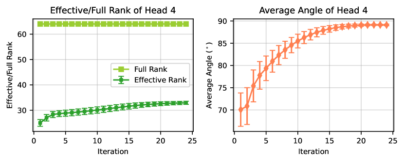
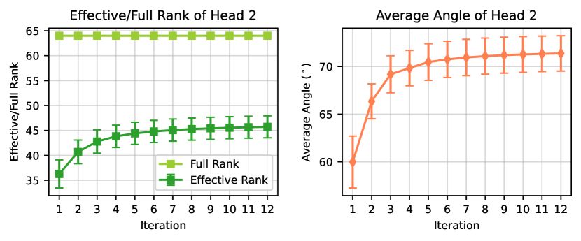
Figure 5: The effective rank and the average angle of tokens projected to one subspace gradually increase, suggesting a larger volume spanned by these tokens. Results are from Sudoku test dataset (Palm et al., 2018) (Top) and CIFAR-10 validation set (Bottom).

Effective Rank & Average Angle. To validate our motivation to mitigate token synchronization in the subspaces, we utilize two metrics to quantify the separation of tokens.

Definition 5.1 (Effective Rank).

For a matrix $\bm{X}\in\mathbb{R}^{d\times N}$, let $\Sigma=[\sigma_{1},\dots,\sigma_{r}]$ be its singular values where $r$ is its full rank and denote $p_{i}=\sigma_{i}/\sum_{j=1}^{r}\sigma_{j}$ the discrete probability. The effective rank (Roy & Vetterli, 2007; Guo et al., 2023) is defined as the exponential of the entropy

$$\exp(-\sum_{i=1}^{r}p_{i}\log p_{i}).$$ (13)

Definition 5.2 (Average Angle).

Given a set of vectors $\bm{X}=[\bm{x}_{1},\dots,\bm{x}_{N}]\in\mathbb{R}^{d\times N}$, the average angle of these vectors is

$$\operatorname{arccos}\frac{2}{N(N-1)}\sum_{i=1}^{N}\sum_{j=i+1}^{N}\frac{\bm{x}_{i}^{T}\bm{x}_{j}}{\|\bm{x}_{i}\|_{2}\|\bm{x}_{j}\|_{2}}.$$ (14)

The effective rank is a continuous approximation of the full rank and, similar to the average angle, reflects the extent to which a set of vectors distributes uniformly. We present the results of these two metrics in Figure 5 (Top) using the token projected to one subspace (1). Full results are in Appendix B.1. As the forward optimization progresses, the effective rank within the subspace steadily rises while the full rank remains unchanged. This dynamic mirrors that of the average angle, which increases from around $70^{\circ}$ to near orthogonal. This implies that tokens in the subspaces occupy maximal hyperspherical volume, and the information encoded in the low dimension gradually saturates.

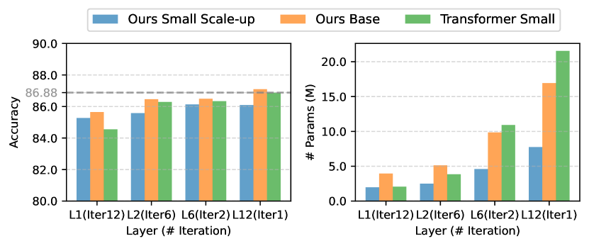
Figure 6: Top-1 Accuracy (Left) and the Number of Parameters (Right) on CIFAR-10 with Different Layer-Iteration Trade-offs.

5.2 Image Classification

Setup & Results. We also evaluate Hyper-SET’s discriminative capability on CIFAR-10, CIFAR-100, and ImageNet-100. We compare against vision Transformers (ViTs), a recently introduced white-box Transformer CRATE (Yu et al., 2023), and its variant CRATE-T that aims for a more faithful implementation (Hu et al., 2024). All models are trained for 200 epochs (batch size 128, 12 iterations, Adam (Kingma, 2014) optimizer, and cosine learning rate decay from 1e-4, no weight decay), with a learnable token $[\texttt{CLS}]$ for classification. Detailed configurations are in Appendix A.3.

As shown in Table 1, with the same hidden dimension, our model surpasses others on CIFAR-10, but underperforms Transformer on CIFAR-100 and ImageNet-100. Noticeably, our architecture can save around $40\%$ of Transformer’s parameters. By scaling up the hidden dimension to match the Transformer’s parameters, our model yields the best result, though performance on ImageNet-100 remains comparable.

Table 1: Top-1 Accuracy on Image Classification. Models are under the same hidden dimension and 12 iterations. Scaling up our model to match Transformer’s parameters gives better performance.

Models	Config ($\#$ Params)	Dataset
		CIFAR-10	CIFAR-100	IM-100
Transformer	Small (2.07 M)	84.55	54.41	57.82
CRATE-T	Small (0.60 M)	78.57	47.55	50.14
CRATE	Small (0.75 M)	80.73	49.25	53.24
Ours	Small (1.24 M)	84.64	54.15	54.78
Ours	Small Scale-up (1.98 M)	85.27	55.94	55.98

Table 2: Comparison of Masked Image Modeling Performance on ImageNet-100 (5k). Our model lags behind Transformer when given the same number of iterations but matches its performance if scaling up the iterations and width of the feedforward module (a.k.a, larger $M$). Our model is also more parameter-efficient.

Models	Layer / Iteration / FF Ratio $M$	PSNR ($\uparrow$)	SSIM ($\uparrow$)	Multi-Scale SSIM ($\uparrow$)	LPIPS ($\downarrow$)	FID ($\downarrow$)
Transformer	1 / 12 / 4$d$  (8.85 M)	15.953	0.417	0.599	0.327	43.428
Ours	1 / 12 / $d$  (3.94 M)	15.713	0.411	0.576	0.358	59.841
Ours	1 / 24 / 8$d$  (8.07 M)	15.955	0.417	0.596	0.332	45.174

Layer-Iteration Trade-off. So far, the classification is conducted under the condition of a one-layer model. A natural question is how well the model will perform when stacking multiple layers with different parameters. To see this, we first run the Transformer with 12 layers, which has the same effective depth as one layer with 12 iterations, as an upper bound. Then, we vary the ratio of distinct layers and their respective iterations while maintaining the effective depth. This configuration can be interpreted as adding flexibility to the basis vectors.

In Figure 6, our scaling-up small model has parameter-efficiency at different layer-iteration ratios, and this strength is significantly sharpened when more independent layers are learned. However, this architectural efficiency limits its scalability beyond two layers. By further scaling to the Base configuration, ours consistently outperforms Transformer even surpassing the upper bound while retaining parameter efficiency.

Energy, Effective Rank & Average Angle. The hyperspherical energy monotonically decreases as in Figure 4 (Bottom) for our Small model with effective rank and average angle mirroring trends from the Sudoku experiment in Figure 5 (Bottom). Complete results are in Appendix B.2.

5.3 Masked Image Modeling

Setup. Masked image modeling has recently reclaimed its attention for autoregressive generation (Li et al., 2023; Chang et al., 2023; Fan et al., 2024; Li et al., 2024), where the generation is framed as recovering images from $100\%$ masking. Due to its high computational demand with large-scale models, we attempt to demonstrate the power of our one-layer model specifically for image reconstruction. ImageNet-100 is used, the same as in Section 5.2. We build on prior work (Chang et al., 2022) and leverage the open-source repository . We follow its setting by using VQ-VAE from (Esser et al., 2021) as the image tokenizer with a codebook size of 1024. See Appendix A.4 for concrete settings.

Results & Visualization. We evaluate the quality of the reconstructed images of masking out $40\%$ of the images with Base configurations. We report Peak Signal-to-Noise Ratio (PSNR), Structural Similarity Index Measure (SSIM), Multi-Scale SSIM, Learned Perceptual Image Patch Similarity (LPIPS) and Fr$\acute{\text{e}}$chet Inception Distance (FID) on the validation set (5k). The results of other ratios and more visualization will be presented in Appendix D.

Numerical results are presented in Table 2. Under the same number of iterations, our model significantly reduces parameters but lags behind Transformer on all metrics. If further increasing its iterations and the width of feedforward module $M$ to 8$d$, it can fill in the performance gap but at the cost of more computation. A visual comparison is in Figure 7.

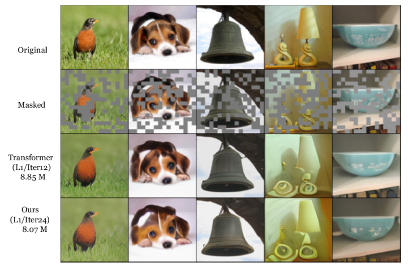
Figure 7: Visual Comparison on Masked Image Modeling on ImageNet 256$\times$256. Our model, when scaling to Transformer scale with additional compute, can achieve similar reconstruction quality when masking ratio $=40\%$.

6 Conclusion

We present Hyper-SET, a Transformer architecture designed via iterative optimization of hyperspherical energy functions, bridging energy-based learning and practical model design. By formulating dual energy objectives on the hypersphere, Hyper-SET mitigates token synchronization in the subspaces while promoting directional alignment with bases in the original space, recovering core Transformer components with intrinsic interpretability. Empirically, Hyper-SET matches or surpasses vanilla Transformers on Sudoku solving, image classification, and masked image modeling tasks with fewer parameters. This work aims to advance principled Transformer design, offering an avenue for building efficient, interpretable architectures grounded in optimization dynamics.

Impact Statement

This paper presents work whose goal is to advance the field of Machine Learning. There are many potential societal consequences of our work, none which we feel must be specifically highlighted here.

Appendix A Detailed Experimental Setup and Model Configuration

A.1 Network to Learn Adaptive Step Size

A.2 Solving Sudoku

Table 4 and Table 4 show the training recipe and model configurations for solving Sudoku. We train the model with 24 iterations and can evaluate beyond these iterations.

Table 3: Training Recipe for Solving Sudoku.

Configuration	Value
Epochs	200
Batch size	16 (on 1 Nvidia 3090 GPU)
Number of training samples	9k
Number of evaluating samples	1k
Optimizer	AdamW ($\beta_{1}=0.0,~\beta_{2}=0.95$)
Weight decay	0.1
Learning rate (lr)	1e-4
Lr decay	Cosine
Gradient clipping	1.0

Table 4: Model Configuration for Solving Sudoku.

Configuration	Value
Vocabulary size	10
Layer	1
Iterations	24
Hidden dimension $d$	768
Feedforward ratio $M$	4$d$
Number of heads $H$	12
Positional encoding	Learnable
Time embedding condition	$\bm{X}_{0}$
Time embedding frequency	512
Number of parameters	5.20 M

A.3 Image Classification

Table 5 and Table 6 present the training recipe and model configurations on image classification, where the number of our model is computed on CIFAR-10. In practice, we use absolute sinusoidal positional encoding and adopt conditioning on $\bm{X}_{t}$ for performance reasons. Table 7 lists the configuration of different sizes and it applies to other tasks as well.

Table 5: Training Recipe for Image Classification.

Configuration	Value
Epochs	200
Batch size	128 (on 1 Nvidia 3090 GPU)
Number of training samples	50k
Number of evaluating samples	10k
Optimizer	Adam ($\beta_{1}=0.0,~\beta_{2}=0.95$)
Weight decay	0.0
Learning rate (lr)	1e-4
Lr decay	Cosine
Gradient clipping	1.0
Input size	224

Table 6: Model Configuration for Image Classification.

Configuration (Small)	Value
Patch size	16
Layer	1
Iterations	12
Hidden dimension $d$	384
Feedforward ratio $M$	$d$
Number of heads $H$	6
Positional encoding	Sinusoidal
Time embedding condition	$\bm{X}_{t}$
Time embedding frequency	512
Number of parameters	1.24 M

Table 7: Model Configuration of Different Sizes

Configurations	Small	Small Scale-up	Base
Hidden dimension $d$	384	512	768
Number of heads $H$	6	8	12

A.4 Masked Image Modeling

We follow (Chang et al., 2022) using VQ-VAE to tokenize the images to $16\times 16$ latent code with codebook size of 1024 after resizing the input to $256\times 256$. Masking ratio is randomly chosen between $[0,0.4]$, and the masked region is replaced by a learnable token. Training loss is computed only for the masked tokens. We also follow the iterative decoding process in (Chang et al., 2022) with $\text{temperature}=1$ and decoding step $T=24$. We also remove the MLP following the time embedding and set the embedding frequency equal to the hidden dimension to save parameters, and we find out that this implementation works better. Table 9 and Table 9 show the detailed training recipe and configurations.

Table 8: Training Recipe for Masked Image Modeling.

Configuration	Value
Epochs	300
Batch size	256 (64 x 4 Nvidia 80 GB A100)
Number of training samples	126,689
Number of evaluating samples	5,000
Optimizer	AdamW ($\beta_{1}=0.0,~\beta_{2}=0.95$)
Weight decay	0.1
Learning rate (lr)	1e-4
Lr decay	None
Gradient clipping	3.0
Input size	256

Table 9: Model Configuration for Masked Image Modeling.

Configuration	Value
Vocabulary size	1025
Layer	1
Iterations	12
Hidden dimension $d$	768
Feedforward ratio $M$	$d$
Number of heads $H$	12
Positional encoding	Sinusoidal
Time embedding condition	$\bm{X}_{0}$
Time embedding frequency	768
Number of parameters	3.94 M

Appendix B Rank and Average Angle of Each Head

B.1 Sudoku Dataset

Figure 9 and Figure 10 capture the evolution of the effective rank and average angle of all heads. Most of them follow the separation dynamics on the hypersphere, mirroring the insights we provide at the beginning of Section B.1.

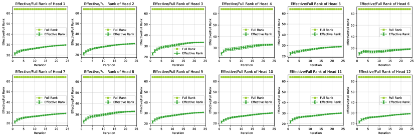
Figure 9: The Effective Rank of Tokens Projected to Each Subspace. Results are from the test set of Sudoku dataset (Palm et al., 2018).

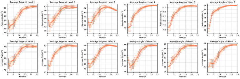
Figure 10: The Average Angle of Tokens Projected to Each Subspace. Results are from the test set of Sudoku dataset (Palm et al., 2018).

B.2 CIFAR-10 Dataset

The full results on CIFAR-10 also possess similar trends to those on the Sudoku dataset as shown in Figure 11 and Figure 12.

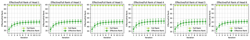
Figure 11: The Effective Rank of Tokens Projected to Each Subspace. Results are from CIFAR-10 validation set.

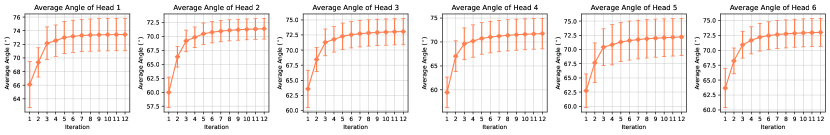
Figure 12: The Average Angle of Tokens Projected to Each Subspace. Results are from CIFAR-10 validation set.

Appendix C Derivation

C.1 Derivation of the Gradient of $E_{\text{ATTN}}$

$$\dot{\bm{x}}_{k} =-\nabla_{\bm{x}_{k}}E_{\text{ATTN}}$$

$$=-\sum_{h=1}^{H}\left(\frac{\sum_{j=1}^{N}\bm{W}_{h}\bm{W}_{h}^{T}\bm{x}_{j}\exp\left(\beta(\bm{W}_{h}^{T}\bm{x}_{k})^{T}(\bm{W}_{h}^{T}\bm{x}_{j})\right)}{\sum_{j=1}^{N}\exp\left(\beta(\bm{W}_{h}^{T}\bm{x}_{k})^{T}(\bm{W}_{h}^{T}\bm{x}_{j})\right)}+\sum_{i=1}^{N}\frac{\bm{W}_{h}\bm{W}_{h}^{T}\bm{x}_{i}\exp\left(\beta(\bm{W}_{h}^{T}\bm{x}_{i})^{T}(\bm{W}_{h}^{T}\bm{x}_{h})\right)}{\sum_{j=1}^{N}\exp\left(\beta(\bm{W}_{h}^{T}\bm{x}_{i})^{T}(\bm{W}_{h}^{T}\bm{x}_{j})\right)}\right)$$

$$=-\sum_{h=1}^{H}\left(\bm{W}_{h}\bm{W}_{h}^{T}[\bm{x}_{1},\dots,\bm{x}_{N}]\begin{bmatrix}\exp\left(\beta(\bm{W}_{h}^{T}\bm{x}_{k})^{T}(\bm{W}_{h}^{T}\bm{x}_{1})\right)\\ \vdots\\ \exp\left(\beta(\bm{W}_{h}^{T}\bm{x}_{k})^{T}(\bm{W}_{h}^{T}\bm{x}_{N})\right)\end{bmatrix}/\sum_{j=1}^{N}\exp\left(\beta(\bm{W}_{h}^{T}\bm{x}_{k})^{T}(\bm{W}_{h}^{T}\bm{x}_{j})\right)+\right.$$

$$\left.\qquad\qquad\qquad\qquad\qquad\qquad\sum_{i=1}^{N}\bm{W}_{h}\bm{W}_{h}^{T}\bm{x}_{i}\begin{bmatrix}\exp\left(\beta(\bm{W}_{h}^{T}\bm{x}_{1})^{T}(\bm{W}_{h}^{T}\bm{x}_{i})\right)/\sum_{j=1}^{N}\exp\left(\beta(\bm{W}_{h}^{T}\bm{x}_{i})^{T}(\bm{W}_{h}^{T}\bm{x}_{j})\right)\\ \vdots\\ \exp\left(\beta(\bm{W}_{h}^{T}\bm{x}_{N})^{T}(\bm{W}_{h}^{T}\bm{x}_{i})\right)/\sum_{j=1}^{N}\exp\left(\beta(\bm{W}_{h}^{T}\bm{x}_{i})^{T}(\bm{W}_{h}^{T}\bm{x}_{j})\right)\end{bmatrix}_{k}\right)$$

$$=-\sum_{h=1}^{H}\left(\bm{W}_{h}\bm{W}_{h}^{T}\bm{X}\underbrace{\operatorname{softmax}}_{\text{column}}\left(\beta(\bm{W}_{h}^{T}\bm{X})^{T}(\bm{W}_{h}^{T}\bm{x}_{k})\right)+\sum_{i=1}^{N}\bm{W}_{h}\bm{W}_{h}^{T}\bm{x}_{i}\underbrace{\operatorname{softmax}}_{\text{column}}\left(\beta(\bm{W}_{h}^{T}\bm{X})^{T}(\bm{W}_{h}^{T}\bm{x}_{i})\right)_{k}\right)$$

$$=-\sum_{h=1}^{H}\left(\bm{W}_{h}\bm{W}_{h}^{T}\bm{X}\underbrace{\operatorname{softmax}}_{\text{column}}\left(\beta(\bm{W}_{h}^{T}\bm{X})^{T}(\bm{W}_{h}^{T}\bm{x}_{k})\right)+\bm{W}_{h}\bm{W}_{h}^{T}[\bm{x}_{1},\dots,\bm{x}_{N}]\underbrace{\operatorname{softmax}}_{\text{column}}\left(\beta(\bm{W}_{h}^{T}\bm{X})^{T}(\bm{W}_{h}^{T}\bm{X})\right)_{[k,:]}\right)$$

$$=-\sum_{h=1}^{H}\left(\bm{W}_{h}\bm{W}_{h}^{T}\bm{X}\underbrace{\operatorname{softmax}}_{\text{column}}\left(\beta(\bm{W}_{h}^{T}\bm{X})^{T}(\bm{W}_{h}^{T}\bm{x}_{k})\right)+\bm{W}_{h}\bm{W}_{h}^{T}[\bm{x}_{1},\dots,\bm{x}_{N}]\underbrace{\operatorname{softmax}}_{\text{row}}\left(\beta(\bm{W}_{h}^{T}\bm{X})^{T}(\bm{W}_{h}^{T}\bm{X})\right)_{[:,k]}\right)$$

$$=-\sum_{h=1}^{H}\left(\bm{W}_{h}\bm{W}_{h}^{T}\bm{X}\underbrace{\operatorname{softmax}}_{\text{column}}\left(\beta(\bm{W}_{h}^{T}\bm{X})^{T}(\bm{W}_{h}^{T}\bm{x}_{k})\right)+\bm{W}_{h}\bm{W}_{h}^{T}\bm{X}\underbrace{\operatorname{softmax}}_{\text{row}}\left(\beta(\bm{W}_{h}^{T}\bm{X})^{T}(\bm{W}_{h}^{T}\bm{X})\right)_{[:,k]}\right)$$

$$\dot{\bm{X}}=[\dot{\bm{x}}_{1},\dots,\dot{\bm{x}}_{N}]=-\nabla_{\bm{X}}E_{\text{ATTN}}=-\left((\bm{W}\bm{W}^{T}\bm{X}\underbrace{\operatorname{softmax}}_{\text{column-wise}}\left(\beta(\bm{W}^{T}\bm{X})^{T}(\bm{W}^{T}\bm{X})\right)+\bm{W}\bm{W}^{T}\bm{X}\underbrace{\operatorname{softmax}}_{\text{row-wise}}\left(\beta(\bm{W}^{T}\bm{X})^{T}(\bm{W}^{T}\bm{X})\right)\right)$$ (15)

C.2 Derivation of the Gradient of $E_{\text{FF}}$

$$\dot{\bm{x}}_{k} =-\nabla_{\bm{x}_{k}}E_{\text{FF}}$$

$$=\sum_{m=1}^{M}\operatorname{ReLU}(\bm{d}_{m}^{T}\bm{x}_{k})\cdot\mathbb{I}(\bm{d}_{m}^{T}\bm{x}_{k}>0)\cdot\bm{d}_{m}$$

$$=\sum_{m=1}^{M}\operatorname{ReLU}(\bm{d}_{m}^{T}\bm{x}_{k})\bm{d}_{m}$$

$$=[\bm{d}_{1},\dots,\bm{d}_{M}]\begin{bmatrix}\operatorname{ReLU}(\bm{d}_{1}^{T}\bm{x}_{k})\\ \vdots\\ \operatorname{ReLU}(\bm{d}_{M}^{T}\bm{x}_{k})\end{bmatrix}$$

$$=\bm{D}\operatorname{ReLU}(\bm{D}^{T}\bm{x}_{k})$$

$$\dot{\bm{X}}=[\dot{\bm{x}}_{1},\dots,\dot{\bm{x}}_{N}]=-\nabla_{\bm{X}}E_{\text{FF}}=\bm{D}\operatorname{ReLU}(\bm{D}^{T}\bm{X})$$

Appendix D Additional Results of Masked Image Modeling

Table 10, Table 11 and Table 12 summarize the results of masked image modeling with different masking ratios. When scaled to larger iterations and a wider feedforward module, our model achieves comparable results to Transformer but still slightly lags behind. This suggests the scalability of our model to the large configuration may be a bottleneck for its development and deployment. More visual comparison is provided in Figure 13.

Table 10: Comparison of Masked Image Modeling Performance of Masking Ratio 0.1.

Models	Layer / Iteration / FF Ratio $M$ (# Params)	PSNR ($\uparrow$)	SSIM ($\uparrow$)	Multi-Scale SSIM ($\uparrow$)	LPIPS ($\downarrow$)	FID ($\downarrow$)
Transformer	L1 / Iter 12 / 4$d$  (8.85 M)	17.693	0.466	0.709	0.236	22.428
Ours	L1 / Iter 12 / $d$  (3.94 M)	17.553	0.462	0.701	0.243	24.665
Ours	L1 / Iter 24 / 8$d$  (8.07 M)	17.673	0.465	0.708	0.236	22.517

Table 11: Comparison of Masked Image Modeling Performance of Masking Ratio 0.2.

Models	Layer / Iteration / FF Ratio $M$ (# Params)	PSNR ($\uparrow$)	SSIM ($\uparrow$)	Multi-Scale SSIM ($\uparrow$)	LPIPS ($\downarrow$)	FID ($\downarrow$)
Transformer	L1 / Iter 12 / 4$d$  (8.85 M)	17.185	0.451	0.678	0.261	27.320
Ours	L1 / Iter 12 / $d$  (3.94 M)	16.988	0.444	0.662	0.275	33.637
Ours	L1 / Iter 24 / 8$d$  (8.07 M)	17.170	0.450	0.676	0.262	28.120

Table 12: Comparison of Masked Image Modeling Performance of Masking Ratio 0.3.

Models	Layer / Iteration / FF Ratio $M$ (# Params)	PSNR ($\uparrow$)	SSIM ($\uparrow$)	Multi-Scale SSIM ($\uparrow$)	LPIPS ($\downarrow$)	FID ($\downarrow$)
Transformer	L1 / Iter 12 / 4$d$  (8.85 M)	16.616	0.435	0.642	0.291	35.095
Ours	L1 / Iter 12 / $d$  (3.94 M)	16.365	0.427	0.621	0.314	45.642
Ours	L1 / Iter 24 / 8$d$  (8.07 M)	16.590	0.434	0.638	0.294	35.128

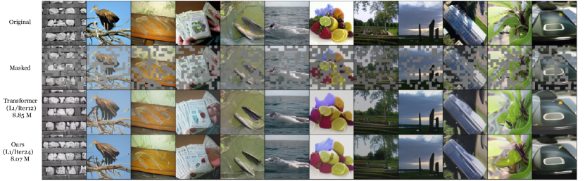
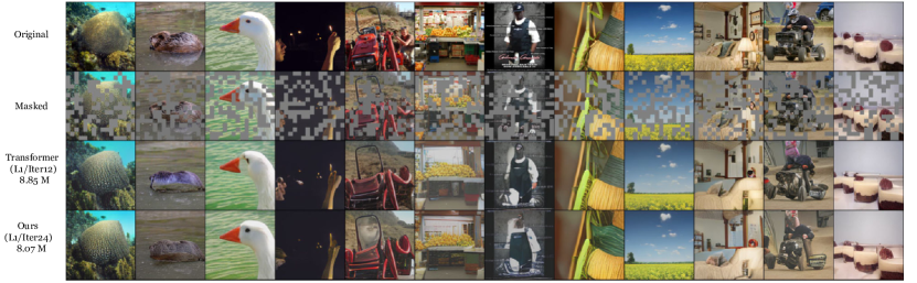
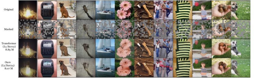
Figure 13: More Comparative Results of Masked Image Modeling on ImageNet 256$\times$256.

References

- Acebrón et al. (2005) Acebrón, J. A., Bonilla, L. L., Pérez Vicente, C. J., Ritort, F., and Spigler, R. The kuramoto model: A simple paradigm for synchronization phenomena. Reviews of modern physics, 77(1):137–185, 2005.
- Ackley et al. (1985) Ackley, D. H., Hinton, G. E., and Sejnowski, T. J. A learning algorithm for boltzmann machines. Cognitive science, 9(1):147–169, 1985.
- Agrawal et al. (2019) Agrawal, A., Amos, B., Barratt, S., Boyd, S., Diamond, S., and Kolter, J. Z. Differentiable convex optimization layers. Advances in neural information processing systems, 32, 2019.
- Amos & Kolter (2017) Amos, B. and Kolter, J. Z. Optnet: Differentiable optimization as a layer in neural networks. In International conference on machine learning, pp. 136–145. PMLR, 2017.
- Amos et al. (2018) Amos, B., Jimenez, I., Sacks, J., Boots, B., and Kolter, J. Z. Differentiable mpc for end-to-end planning and control. Advances in neural information processing systems, 31, 2018.
- Anil et al. (2023) Anil, R., Borgeaud, S., Wu, Y., Alayrac, J.-B., Yu, J., Soricut, R., Schalkwyk, J., Dai, A. M., Hauth, A., Millican, K., et al. Gemini: A family of highly capable multimodal models. arXiv preprint arXiv:2312.11805, 1, 2023.
- Bachlechner et al. (2021) Bachlechner, T., Majumder, B. P., Mao, H., Cottrell, G., and McAuley, J. Rezero is all you need: Fast convergence at large depth. In Uncertainty in Artificial Intelligence, pp. 1352–1361. PMLR, 2021.
- Bai et al. (2019) Bai, S., Kolter, J. Z., and Koltun, V. Deep equilibrium models. Advances in neural information processing systems, 32, 2019.
- Banino et al. (2021) Banino, A., Balaguer, J., and Blundell, C. Pondernet: Learning to ponder. In 8th ICML Workshop on Automated Machine Learning (AutoML), 2021. URL https://openreview.net/forum?id=1EuxRTe0WN.
- Bansal et al. (2022) Bansal, A., Schwarzschild, A., Borgnia, E., Emam, Z., Huang, F., Goldblum, M., and Goldstein, T. End-to-end algorithm synthesis with recurrent networks: Extrapolation without overthinking. Advances in Neural Information Processing Systems, 35:20232–20242, 2022.
- Bao et al. (2022) Bao, H., Dong, L., Piao, S., and Wei, F. BEit: BERT pre-training of image transformers. In International Conference on Learning Representations, 2022. URL https://openreview.net/forum?id=p-BhZSz59o4.
- Bietti et al. (2023) Bietti, A., Cabannes, V., Bouchacourt, D., Jegou, H., and Bottou, L. Birth of a transformer: A memory viewpoint. In Thirty-seventh Conference on Neural Information Processing Systems, 2023. URL https://openreview.net/forum?id=3X2EbBLNsk.
- Bricken & Pehlevan (2021) Bricken, T. and Pehlevan, C. Attention approximates sparse distributed memory. Advances in Neural Information Processing Systems, 34:15301–15315, 2021.
- Bricken et al. (2023) Bricken, T., Templeton, A., Batson, J., Chen, B., Jermyn, A., Conerly, T., Turner, N., Anil, C., Denison, C., Askell, A., Lasenby, R., Wu, Y., Kravec, S., Schiefer, N., Maxwell, T., Joseph, N., Hatfield-Dodds, Z., Tamkin, A., Nguyen, K., McLean, B., Burke, J. E., Hume, T., Carter, S., Henighan, T., and Olah, C. Towards monosemanticity: Decomposing language models with dictionary learning. Transformer Circuits Thread, 2023. https://transformer-circuits.pub/2023/monosemantic-features/index.html.
- Brohan et al. (2022) Brohan, A., Brown, N., Carbajal, J., Chebotar, Y., Dabis, J., Finn, C., Gopalakrishnan, K., Hausman, K., Herzog, A., Hsu, J., et al. Rt-1: Robotics transformer for real-world control at scale. arXiv preprint arXiv:2212.06817, 2022.
- Brown et al. (2020) Brown, T., Mann, B., Ryder, N., Subbiah, M., Kaplan, J. D., Dhariwal, P., Neelakantan, A., Shyam, P., Sastry, G., Askell, A., et al. Language models are few-shot learners. Advances in neural information processing systems, 33:1877–1901, 2020.
- Chang et al. (2022) Chang, H., Zhang, H., Jiang, L., Liu, C., and Freeman, W. T. Maskgit: Masked generative image transformer. In Proceedings of the IEEE/CVF Conference on Computer Vision and Pattern Recognition, pp. 11315–11325, 2022.
- Chang et al. (2023) Chang, H., Zhang, H., Barber, J., Maschinot, A., Lezama, J., Jiang, L., Yang, M.-H., Murphy, K. P., Freeman, W. T., Rubinstein, M., Li, Y., and Krishnan, D. Muse: Text-to-image generation via masked generative transformers. In Krause, A., Brunskill, E., Cho, K., Engelhardt, B., Sabato, S., and Scarlett, J. (eds.), Proceedings of the 40th International Conference on Machine Learning, volume 202 of Proceedings of Machine Learning Research, pp. 4055–4075. PMLR, 23–29 Jul 2023. URL https://proceedings.mlr.press/v202/chang23b.html.
- Chen et al. (2021) Chen, L., Lu, K., Rajeswaran, A., Lee, K., Grover, A., Laskin, M., Abbeel, P., Srinivas, A., and Mordatch, I. Decision transformer: Reinforcement learning via sequence modeling. Advances in neural information processing systems, 34:15084–15097, 2021.
- Chen et al. (2022) Chen, T., Zhang, Z., Cheng, Y., Awadallah, A., and Wang, Z. The principle of diversity: Training stronger vision transformers calls for reducing all levels of redundancy. In Proceedings of the IEEE/CVF Conference on Computer Vision and Pattern Recognition, pp. 12020–12030, 2022.
- Conmy et al. (2023) Conmy, A., Mavor-Parker, A., Lynch, A., Heimersheim, S., and Garriga-Alonso, A. Towards automated circuit discovery for mechanistic interpretability. Advances in Neural Information Processing Systems, 36:16318–16352, 2023.
- Dawid & LeCun (2024) Dawid, A. and LeCun, Y. Introduction to latent variable energy-based models: a path toward autonomous machine intelligence. Journal of Statistical Mechanics: Theory and Experiment, 2024(10):104011, 2024.
- Devlin et al. (2019) Devlin, J., Chang, M.-W., Lee, K., and Toutanova, K. BERT: Pre-training of deep bidirectional transformers for language understanding. In Burstein, J., Doran, C., and Solorio, T. (eds.), Proceedings of the 2019 Conference of the North American Chapter of the Association for Computational Linguistics: Human Language Technologies, Volume 1 (Long and Short Papers), pp. 4171–4186, Minneapolis, Minnesota, June 2019. Association for Computational Linguistics. doi: 10.18653/v1/N19-1423. URL https://aclanthology.org/N19-1423/.
- Dong et al. (2021) Dong, Y., Cordonnier, J.-B., and Loukas, A. Attention is not all you need: pure attention loses rank doubly exponentially with depth. In Meila, M. and Zhang, T. (eds.), Proceedings of the 38th International Conference on Machine Learning, volume 139 of Proceedings of Machine Learning Research, pp. 2793–2803. PMLR, 18–24 Jul 2021.
- Dosovitskiy et al. (2021) Dosovitskiy, A., Beyer, L., Kolesnikov, A., Weissenborn, D., Zhai, X., Unterthiner, T., Dehghani, M., Minderer, M., Heigold, G., Gelly, S., Uszkoreit, J., and Houlsby, N. An image is worth 16x16 words: Transformers for image recognition at scale. In International Conference on Learning Representations, 2021. URL https://openreview.net/forum?id=YicbFdNTTy.
- Du & Mordatch (2019) Du, Y. and Mordatch, I. Implicit generation and modeling with energy based models. Advances in Neural Information Processing Systems, 32, 2019.
- Du et al. (2022) Du, Y., Li, S., Tenenbaum, J., and Mordatch, I. Learning iterative reasoning through energy minimization. In International Conference on Machine Learning, pp. 5570–5582. PMLR, 2022.
- Dubey et al. (2024) Dubey, A., Jauhri, A., Pandey, A., Kadian, A., Al-Dahle, A., Letman, A., Mathur, A., Schelten, A., Yang, A., Fan, A., et al. The llama 3 herd of models. arXiv preprint arXiv:2407.21783, 2024.
- Elhage et al. (2021) Elhage, N., Nanda, N., Olsson, C., Henighan, T., Joseph, N., Mann, B., Askell, A., Bai, Y., Chen, A., Conerly, T., et al. A mathematical framework for transformer circuits. Transformer Circuits Thread, 1(1):12, 2021.
- Esser et al. (2021) Esser, P., Rombach, R., and Ommer, B. Taming transformers for high-resolution image synthesis. In Proceedings of the IEEE/CVF conference on computer vision and pattern recognition, pp. 12873–12883, 2021.
- Fan et al. (2024) Fan, L., Li, T., Qin, S., Li, Y., Sun, C., Rubinstein, M., Sun, D., He, K., and Tian, Y. Fluid: Scaling autoregressive text-to-image generative models with continuous tokens. arXiv preprint arXiv:2410.13863, 2024.
- Geshkovski et al. (2023a) Geshkovski, B., Letrouit, C., Polyanskiy, Y., and Rigollet, P. A mathematical perspective on transformers. arXiv preprint arXiv:2312.10794, 2023a.
- Geshkovski et al. (2023b) Geshkovski, B., Letrouit, C., Polyanskiy, Y., and Rigollet, P. The emergence of clusters in self-attention dynamics. In Thirty-seventh Conference on Neural Information Processing Systems, 2023b. URL https://openreview.net/forum?id=aMjaEkkXJx.
- Gregor & LeCun (2010) Gregor, K. and LeCun, Y. Learning fast approximations of sparse coding. In Proceedings of the 27th international conference on international conference on machine learning, pp. 399–406, 2010.
- Greydanus et al. (2019) Greydanus, S., Dzamba, M., and Yosinski, J. Hamiltonian neural networks. Advances in neural information processing systems, 32, 2019.
- Gromov et al. (2024) Gromov, A., Tirumala, K., Shapourian, H., Glorioso, P., and Roberts, D. A. The unreasonable ineffectiveness of the deeper layers. arXiv preprint arXiv:2403.17887, 2024.
- Guo et al. (2023) Guo, X., Wang, Y., Du, T., and Wang, Y. Contranorm: A contrastive learning perspective on oversmoothing and beyond. In The Eleventh International Conference on Learning Representations, 2023. URL https://openreview.net/forum?id=SM7XkJouWHm.
- He et al. (2022) He, K., Chen, X., Xie, S., Li, Y., Dollár, P., and Girshick, R. Masked autoencoders are scalable vision learners. In Proceedings of the IEEE/CVF conference on computer vision and pattern recognition, pp. 16000–16009, 2022.
- Henry et al. (2020) Henry, A., Dachapally, P. R., Pawar, S. S., and Chen, Y. Query-key normalization for transformers. In Cohn, T., He, Y., and Liu, Y. (eds.), Findings of the Association for Computational Linguistics: EMNLP 2020, pp. 4246–4253, Online, November 2020. Association for Computational Linguistics. doi: 10.18653/v1/2020.findings-emnlp.379. URL https://aclanthology.org/2020.findings-emnlp.379/.
- Hoover et al. (2024) Hoover, B., Liang, Y., Pham, B., Panda, R., Strobelt, H., Chau, D. H., Zaki, M., and Krotov, D. Energy transformer. Advances in Neural Information Processing Systems, 36, 2024.
- Hopfield (1982) Hopfield, J. J. Neural networks and physical systems with emergent collective computational abilities. Proceedings of the national academy of sciences, 79(8):2554–2558, 1982.
- Hu et al. (2024) Hu, Y., Zou, D., and Xu, D. An in-depth investigation of sparse rate reduction in transformer-like models. In The Thirty-eighth Annual Conference on Neural Information Processing Systems, 2024. URL https://openreview.net/forum?id=CAC74VuMWX.
- Huben et al. (2024) Huben, R., Cunningham, H., Smith, L. R., Ewart, A., and Sharkey, L. Sparse autoencoders find highly interpretable features in language models. In The Twelfth International Conference on Learning Representations, 2024. URL https://openreview.net/forum?id=F76bwRSLeK.
- Jumper et al. (2021) Jumper, J., Evans, R., Pritzel, A., Green, T., Figurnov, M., Ronneberger, O., Tunyasuvunakool, K., Bates, R., Žídek, A., Potapenko, A., et al. Highly accurate protein structure prediction with alphafold. nature, 596(7873):583–589, 2021.
- Kamienny et al. (2022) Kamienny, P.-A., d’Ascoli, S., Lample, G., and Charton, F. End-to-end symbolic regression with transformers. Advances in Neural Information Processing Systems, 35:10269–10281, 2022.
- Kaplan et al. (2020) Kaplan, J., McCandlish, S., Henighan, T., Brown, T. B., Chess, B., Child, R., Gray, S., Radford, A., Wu, J., and Amodei, D. Scaling laws for neural language models, 2020. URL https://arxiv.org/abs/2001.08361.
- Karniadakis et al. (2021) Karniadakis, G. E., Kevrekidis, I. G., Lu, L., Perdikaris, P., Wang, S., and Yang, L. Physics-informed machine learning. Nature Reviews Physics, 3(6):422–440, 2021.
- Kingma (2014) Kingma, D. P. Adam: A method for stochastic optimization. arXiv preprint arXiv:1412.6980, 2014.
- Kozachkov et al. (2023) Kozachkov, L., Kastanenka, K. V., and Krotov, D. Building transformers from neurons and astrocytes. Proceedings of the National Academy of Sciences, 120(34):e2219150120, 2023.
- Krotov (2023) Krotov, D. A new frontier for hopfield networks. Nature Reviews Physics, 5(7):366–367, 2023.
- Krotov & Hopfield (2016) Krotov, D. and Hopfield, J. J. Dense associative memory for pattern recognition. Advances in neural information processing systems, 29, 2016.
- Krotov & Hopfield (2021) Krotov, D. and Hopfield, J. J. Large associative memory problem in neurobiology and machine learning. In International Conference on Learning Representations, 2021. URL https://openreview.net/forum?id=X4y_10OX-hX.
- Lad et al. (2024) Lad, V., Gurnee, W., and Tegmark, M. The remarkable robustness of llms: Stages of inference? arXiv preprint arXiv:2406.19384, 2024.
- Lan et al. (2020) Lan, Z., Chen, M., Goodman, S., Gimpel, K., Sharma, P., and Soricut, R. Albert: A lite bert for self-supervised learning of language representations. In International Conference on Learning Representations, 2020. URL https://openreview.net/forum?id=H1eA7AEtvS.
- LeCun et al. (2006) LeCun, Y., Chopra, S., Hadsell, R., et al. A tutorial on energy-based learning. 2006.
- Li et al. (2023) Li, T., Chang, H., Mishra, S., Zhang, H., Katabi, D., and Krishnan, D. Mage: Masked generative encoder to unify representation learning and image synthesis. In Proceedings of the IEEE/CVF Conference on Computer Vision and Pattern Recognition, pp. 2142–2152, 2023.
- Li et al. (2024) Li, T., Tian, Y., Li, H., Deng, M., and He, K. Autoregressive image generation without vector quantization. In The Thirty-eighth Annual Conference on Neural Information Processing Systems, 2024. URL https://openreview.net/forum?id=VNBIF0gmkb.
- Liu et al. (2018) Liu, W., Lin, R., Liu, Z., Liu, L., Yu, Z., Dai, B., and Song, L. Learning towards minimum hyperspherical energy. Advances in neural information processing systems, 31, 2018.
- Liu et al. (2024) Liu, Z., Wang, Y., Vaidya, S., Ruehle, F., Halverson, J., Soljačić, M., Hou, T. Y., and Tegmark, M. Kan: Kolmogorov-arnold networks. arXiv preprint arXiv:2404.19756, 2024.
- Loshchilov & Hutter (2019) Loshchilov, I. and Hutter, F. Decoupled weight decay regularization. In International Conference on Learning Representations, 2019. URL https://openreview.net/forum?id=Bkg6RiCqY7.
- Loshchilov et al. (2024) Loshchilov, I., Hsieh, C.-P., Sun, S., and Ginsburg, B. ngpt: Normalized transformer with representation learning on the hypersphere. arXiv preprint arXiv:2410.01131, 2024.
- Men et al. (2024) Men, X., Xu, M., Zhang, Q., Wang, B., Lin, H., Lu, Y., Han, X., and Chen, W. Shortgpt: Layers in large language models are more redundant than you expect. arXiv preprint arXiv:2403.03853, 2024.
- Meng et al. (2022) Meng, K., Bau, D., Andonian, A., and Belinkov, Y. Locating and editing factual associations in gpt. Advances in Neural Information Processing Systems, 35:17359–17372, 2022.
- Miyato et al. (2024) Miyato, T., Löwe, S., Geiger, A., and Welling, M. Artificial kuramoto oscillatory neurons. arXiv preprint arXiv:2410.13821, 2024.
- Nanda et al. (2023) Nanda, N., Chan, L., Lieberum, T., Smith, J., and Steinhardt, J. Progress measures for grokking via mechanistic interpretability. In The Eleventh International Conference on Learning Representations, 2023. URL https://openreview.net/forum?id=9XFSbDPmdW.
- Olsson et al. (2022) Olsson, C., Elhage, N., Nanda, N., Joseph, N., DasSarma, N., Henighan, T., Mann, B., Askell, A., Bai, Y., Chen, A., Conerly, T., Drain, D., Ganguli, D., Hatfield-Dodds, Z., Hernandez, D., Johnston, S., Jones, A., Kernion, J., Lovitt, L., Ndousse, K., Amodei, D., Brown, T., Clark, J., Kaplan, J., McCandlish, S., and Olah, C. In-context learning and induction heads. Transformer Circuits Thread, 2022. https://transformer-circuits.pub/2022/in-context-learning-and-induction-heads/index.html.
- OpenAI et al. (2024) OpenAI, Achiam, J., Adler, S., Agarwal, S., Ahmad, L., Akkaya, I., Aleman, F. L., Almeida, D., Altenschmidt, J., Altman, S., Anadkat, S., Avila, R., Babuschkin, I., Balaji, S., Balcom, V., Baltescu, P., Bao, H., Bavarian, M., Belgum, J., Bello, I., Berdine, J., Bernadett-Shapiro, G., Berner, C., Bogdonoff, L., Boiko, O., Boyd, M., Brakman, A.-L., Brockman, G., Brooks, T., Brundage, M., Button, K., Cai, T., Campbell, R., Cann, A., Carey, B., Carlson, C., Carmichael, R., Chan, B., Chang, C., Chantzis, F., Chen, D., Chen, S., Chen, R., Chen, J., Chen, M., Chess, B., Cho, C., Chu, C., Chung, H. W., Cummings, D., Currier, J., Dai, Y., Decareaux, C., Degry, T., Deutsch, N., Deville, D., Dhar, A., Dohan, D., Dowling, S., Dunning, S., Ecoffet, A., Eleti, A., Eloundou, T., Farhi, D., Fedus, L., Felix, N., Fishman, S. P., Forte, J., Fulford, I., Gao, L., Georges, E., Gibson, C., Goel, V., Gogineni, T., Goh, G., Gontijo-Lopes, R., Gordon, J., Grafstein, M., Gray, S., Greene, R., Gross, J., Gu, S. S., Guo, Y., Hallacy, C., Han, J., Harris, J., He, Y., Heaton, M., Heidecke, J., Hesse, C., Hickey, A., Hickey, W., Hoeschele, P., Houghton, B., Hsu, K., Hu, S., Hu, X., Huizinga, J., Jain, S., Jain, S., Jang, J., Jiang, A., Jiang, R., Jin, H., Jin, D., Jomoto, S., Jonn, B., Jun, H., Kaftan, T., Łukasz Kaiser, Kamali, A., Kanitscheider, I., Keskar, N. S., Khan, T., Kilpatrick, L., Kim, J. W., Kim, C., Kim, Y., Kirchner, J. H., Kiros, J., Knight, M., Kokotajlo, D., Łukasz Kondraciuk, Kondrich, A., Konstantinidis, A., Kosic, K., Krueger, G., Kuo, V., Lampe, M., Lan, I., Lee, T., Leike, J., Leung, J., Levy, D., Li, C. M., Lim, R., Lin, M., Lin, S., Litwin, M., Lopez, T., Lowe, R., Lue, P., Makanju, A., Malfacini, K., Manning, S., Markov, T., Markovski, Y., Martin, B., Mayer, K., Mayne, A., McGrew, B., McKinney, S. M., McLeavey, C., McMillan, P., McNeil, J., Medina, D., Mehta, A., Menick, J., Metz, L., Mishchenko, A., Mishkin, P., Monaco, V., Morikawa, E., Mossing, D., Mu, T., Murati, M., Murk, O., Mély, D., Nair, A., Nakano, R., Nayak, R., Neelakantan, A., Ngo, R., Noh, H., Ouyang, L., O’Keefe, C., Pachocki, J., Paino, A., Palermo, J., Pantuliano, A., Parascandolo, G., Parish, J., Parparita, E., Passos, A., Pavlov, M., Peng, A., Perelman, A., de Avila Belbute Peres, F., Petrov, M., de Oliveira Pinto, H. P., Michael, Pokorny, Pokrass, M., Pong, V. H., Powell, T., Power, A., Power, B., Proehl, E., Puri, R., Radford, A., Rae, J., Ramesh, A., Raymond, C., Real, F., Rimbach, K., Ross, C., Rotsted, B., Roussez, H., Ryder, N., Saltarelli, M., Sanders, T., Santurkar, S., Sastry, G., Schmidt, H., Schnurr, D., Schulman, J., Selsam, D., Sheppard, K., Sherbakov, T., Shieh, J., Shoker, S., Shyam, P., Sidor, S., Sigler, E., Simens, M., Sitkin, J., Slama, K., Sohl, I., Sokolowsky, B., Song, Y., Staudacher, N., Such, F. P., Summers, N., Sutskever, I., Tang, J., Tezak, N., Thompson, M. B., Tillet, P., Tootoonchian, A., Tseng, E., Tuggle, P., Turley, N., Tworek, J., Uribe, J. F. C., Vallone, A., Vijayvergiya, A., Voss, C., Wainwright, C., Wang, J. J., Wang, A., Wang, B., Ward, J., Wei, J., Weinmann, C., Welihinda, A., Welinder, P., Weng, J., Weng, L., Wiethoff, M., Willner, D., Winter, C., Wolrich, S., Wong, H., Workman, L., Wu, S., Wu, J., Wu, M., Xiao, K., Xu, T., Yoo, S., Yu, K., Yuan, Q., Zaremba, W., Zellers, R., Zhang, C., Zhang, M., Zhao, S., Zheng, T., Zhuang, J., Zhuk, W., and Zoph, B. Gpt-4 technical report, 2024. URL https://arxiv.org/abs/2303.08774.
- Oquab et al. (2024) Oquab, M., Darcet, T., Moutakanni, T., Vo, H. V., Szafraniec, M., Khalidov, V., Fernandez, P., HAZIZA, D., Massa, F., El-Nouby, A., Assran, M., Ballas, N., Galuba, W., Howes, R., Huang, P.-Y., Li, S.-W., Misra, I., Rabbat, M., Sharma, V., Synnaeve, G., Xu, H., Jegou, H., Mairal, J., Labatut, P., Joulin, A., and Bojanowski, P. DINOv2: Learning robust visual features without supervision. Transactions on Machine Learning Research, 2024. ISSN 2835-8856. URL https://openreview.net/forum?id=a68SUt6zFt. Featured Certification.
- Palm et al. (2018) Palm, R., Paquet, U., and Winther, O. Recurrent relational networks. Advances in neural information processing systems, 31, 2018.
- Papyan et al. (2017) Papyan, V., Romano, Y., and Elad, M. Convolutional neural networks analyzed via convolutional sparse coding. Journal of Machine Learning Research, 18(83):1–52, 2017.
- Papyan et al. (2018) Papyan, V., Romano, Y., Sulam, J., and Elad, M. Theoretical foundations of deep learning via sparse representations: A multilayer sparse model and its connection to convolutional neural networks. IEEE Signal Processing Magazine, 35(4):72–89, 2018.
- Peebles & Xie (2023) Peebles, W. and Xie, S. Scalable diffusion models with transformers. In Proceedings of the IEEE/CVF International Conference on Computer Vision, pp. 4195–4205, 2023.
- Ramsauer et al. (2021) Ramsauer, H., Schäfl, B., Lehner, J., Seidl, P., Widrich, M., Gruber, L., Holzleitner, M., Adler, T., Kreil, D., Kopp, M. K., Klambauer, G., Brandstetter, J., and Hochreiter, S. Hopfield networks is all you need. In International Conference on Learning Representations, 2021. URL https://openreview.net/forum?id=tL89RnzIiCd.
- Roy & Vetterli (2007) Roy, O. and Vetterli, M. The effective rank: A measure of effective dimensionality. In 2007 15th European signal processing conference, pp. 606–610. IEEE, 2007.
- Sander et al. (2022) Sander, M. E., Ablin, P., Blondel, M., and Peyré, G. Sinkformers: Transformers with doubly stochastic attention. In Camps-Valls, G., Ruiz, F. J. R., and Valera, I. (eds.), Proceedings of The 25th International Conference on Artificial Intelligence and Statistics, volume 151 of Proceedings of Machine Learning Research, pp. 3515–3530. PMLR, 28–30 Mar 2022. URL https://proceedings.mlr.press/v151/sander22a.html.
- Scarlett et al. (2022) Scarlett, J., Heckel, R., Rodrigues, M. R., Hand, P., and Eldar, Y. C. Theoretical perspectives on deep learning methods in inverse problems. IEEE journal on selected areas in information theory, 3(3):433–453, 2022.
- Schwarzschild et al. (2021) Schwarzschild, A., Borgnia, E., Gupta, A., Huang, F., Vishkin, U., Goldblum, M., and Goldstein, T. Can you learn an algorithm? generalizing from easy to hard problems with recurrent networks. Advances in Neural Information Processing Systems, 34:6695–6706, 2021.
- Shlezinger et al. (2023) Shlezinger, N., Whang, J., Eldar, Y. C., and Dimakis, A. G. Model-based deep learning. Proceedings of the IEEE, 111(5):465–499, 2023.
- Sohl-Dickstein et al. (2015) Sohl-Dickstein, J., Weiss, E., Maheswaranathan, N., and Ganguli, S. Deep unsupervised learning using nonequilibrium thermodynamics. In Bach, F. and Blei, D. (eds.), Proceedings of the 32nd International Conference on Machine Learning, volume 37 of Proceedings of Machine Learning Research, pp. 2256–2265, Lille, France, 07–09 Jul 2015. PMLR. URL https://proceedings.mlr.press/v37/sohl-dickstein15.html.
- Song & Ermon (2019) Song, Y. and Ermon, S. Generative modeling by estimating gradients of the data distribution. Advances in neural information processing systems, 32, 2019.
- Song et al. (2021) Song, Y., Sohl-Dickstein, J., Kingma, D. P., Kumar, A., Ermon, S., and Poole, B. Score-based generative modeling through stochastic differential equations. In International Conference on Learning Representations, 2021. URL https://openreview.net/forum?id=PxTIG12RRHS.
- Sun et al. (2024) Sun, Q., Pickett, M., Nain, A. K., and Jones, L. Transformer layers as painters. arXiv preprint arXiv:2407.09298, 2024.
- Thuerey et al. (2021) Thuerey, N., Holl, P., Mueller, M., Schnell, P., Trost, F., and Um, K. Physics-based deep learning. arXiv preprint arXiv:2109.05237, 2021.
- Tishby & Zaslavsky (2015) Tishby, N. and Zaslavsky, N. Deep learning and the information bottleneck principle. In 2015 ieee information theory workshop (itw), pp. 1–5. IEEE, 2015.
- Tishby et al. (2000) Tishby, N., Pereira, F. C., and Bialek, W. The information bottleneck method. arXiv preprint physics/0004057, 2000.
- Touvron et al. (2021) Touvron, H., Cord, M., Sablayrolles, A., Synnaeve, G., and Jégou, H. Going deeper with image transformers. In Proceedings of the IEEE/CVF international conference on computer vision, pp. 32–42, 2021.
- Vaswani et al. (2017) Vaswani, A., Shazeer, N., Parmar, N., Uszkoreit, J., Jones, L., Gomez, A. N., Kaiser, L. u., and Polosukhin, I. Attention is all you need. In Guyon, I., Luxburg, U. V., Bengio, S., Wallach, H., Fergus, R., Vishwanathan, S., and Garnett, R. (eds.), Advances in Neural Information Processing Systems, volume 30. Curran Associates, Inc., 2017. URL https://proceedings.neurips.cc/paper_files/paper/2017/file/3f5ee243547dee91fbd053c1c4a845aa-Paper.pdf.
- Vershynin (2018) Vershynin, R. High-dimensional probability: An introduction with applications in data science, volume 47. Cambridge university press, 2018.
- Vig et al. (2020) Vig, J., Gehrmann, S., Belinkov, Y., Qian, S., Nevo, D., Singer, Y., and Shieber, S. Investigating gender bias in language models using causal mediation analysis. Advances in neural information processing systems, 33:12388–12401, 2020.
- Wang et al. (2023) Wang, K. R., Variengien, A., Conmy, A., Shlegeris, B., and Steinhardt, J. Interpretability in the wild: a circuit for indirect object identification in GPT-2 small. In The Eleventh International Conference on Learning Representations, 2023. URL https://openreview.net/forum?id=NpsVSN6o4ul.
- Wang et al. (2019) Wang, P.-W., Donti, P., Wilder, B., and Kolter, Z. Satnet: Bridging deep learning and logical reasoning using a differentiable satisfiability solver. In International Conference on Machine Learning, pp. 6545–6554. PMLR, 2019.
- Wu et al. (2024) Wu, X., Ajorlou, A., Wu, Z., and Jadbabaie, A. Demystifying oversmoothing in attention-based graph neural networks. Advances in Neural Information Processing Systems, 36, 2024.
- Yang et al. (2021) Yang, Y., Liu, T., Wang, Y., Zhou, J., Gan, Q., Wei, Z., Zhang, Z., Huang, Z., and Wipf, D. Graph neural networks inspired by classical iterative algorithms. In International Conference on Machine Learning, pp. 11773–11783. PMLR, 2021.
- Yang et al. (2023) Yang, Z., Ishay, A., and Lee, J. Learning to solve constraint satisfaction problems with recurrent transformer. In The Eleventh International Conference on Learning Representations, 2023. URL https://openreview.net/forum?id=udNhDCr2KQe.
- Yu et al. (2023) Yu, Y., Buchanan, S., Pai, D., Chu, T., Wu, Z., Tong, S., Haeffele, B., and Ma, Y. White-box transformers via sparse rate reduction. Advances in Neural Information Processing Systems, 36:9422–9457, 2023.
- Yuille & Rangarajan (2003) Yuille, A. L. and Rangarajan, A. The concave-convex procedure. Neural computation, 15(4):915–936, 2003.