O-MMGP: Optimal Mesh Morphing Gaussian Process Regression for Solving PDEs with non-Parametric Geometric Variations

Abstract

We address the computational challenges of solving parametric PDEs with non parametrized geometric variations and non-reducible problems, such as those involving shocks and discontinuities of variable positions. Traditional dimensionality reduction methods like POD struggle with these scenarios due to slowly decaying Kolmogorov widths. To overcome this, we propose a novel non-linear dimensionality reduction technique to reduce the required modes for representation. The non-linear reduction is obtained through a POD after applying a transformation on the fields, which we call optimal mappings, and is a solution to an optimization problem in infinite dimension. The proposed learning framework combines morphing techniques, non-linear dimensionality reduction, and Gaussian Process Regression (GPR). The problem is reformulated on a reference geometry before applying the dimensionality reduction. Our method learns both the optimal mapping, and the solution fields, using a series of GPR models, enabling efficient and accurate modeling of complex parametric PDEs with geometrical variability. The results obtained concur with current state-of-the-art models. We mainly compare our method with the winning solution of the ML4CFD NeurIPS 2024 competition.

1 Introduction

1.1 Background

Many scientific and engineering challenges involve solving complex boundary value problems, often formulated as parametric partial differential equations (PDEs). These problems require exploring the influence of varying parameters such as material properties, boundary and initial conditions, or geometric configurations. Traditional numerical methods like the finite element method and finite difference methods, while accurate, are computationally expensive, particularly when repeated evaluations are necessary across a large and high-dimensional parameter set. To address this computational burden, techniques in model-order reduction and machine learning have been developed, offering efficient approximations without compromising accuracy.

Model-order reduction techniques, such as the reduced-basis method [25, 14], construct low-dimensional approximation vector spaces to represent the set of solutions of the parametric PDE, enabling fast computation for new parameter values. These approaches typically involve an offline phase, where high-fidelity models are used to generate a reduced basis, and an online phase, where this basis is employed for efficient computations. However, when the physical domain varies with the parameters, standard methods like Proper Orthogonal Decomposition (POD) face challenges due to the need to reconcile solutions defined on different domains. This often requires morphing techniques to map variable domains to a common one, transforming the problem into a form suitable for reduced-order modeling [21, 28]. Linear reduced-order modeling techniques also face huge difficulties when the solution set of interest has a slowly decaying Kolmogorov width. Such problems, which we call herefafter non-reducible problems, are common for PDEs that involve shocks of variable position, discontinuities, boundary layers an so on.

On the other hand, machine learning methods, particularly those relying on deep learning, have shown promise in solving PDEs, learning solutions, and accelerating computations [13, 19]. Approaches relying on graph neural networks (GNNs) [29] have been particularly effective in handling unstructured meshes and varying geometric configurations. Despite their flexibility, these methods require substantial computational resources and large training datasets, and they often lack robust predictive uncertainty estimates.

1.2 Contribution

In this work, we propose a novel approach that integrates principles of morphing, non-linear dimensionality reduction, and classical machine learning to address the challenges posed by parametric PDEs with geometric variations for non-reducible problems. The main contribution is a novel algorithm used to minimize the number of modes needed to approximate non-reducible problems in moderate dimension. Such approaches are commonly called registration in the literature. Unlike most exsiting algorithms that aim at projecting the samples on one single mode, our approach is based on the resolution of an optimization problem in infinite dimension that may involve an arbitrary number of modes $r\in\mathbb{N}^{*}$, allowing topology changes in the fields of interest.

1.3 Related works

The challenges mentioned in this work have been extensively studied in the literature. Morphing techniques have been used for various applications in reduced order modeling to recast the problem on a reference domain [24, 1, 35]. Numerous approaches were also proposed to deal with non-reducible problems by using non-linear dimensionality reduction such as registration [30, 32], feature tracking [22], optimal transport [9], neural networks [16, 12, 3, 5], and so on. Machine learning approaches leveraging neural networks have also demonstrated remarkable success in solving numerical simulations, particularly in capturing complex patterns and dynamics. Methods such as the Fourier Neural Operator (FNO) [18] and its extension, Geo-FNO [17], efficiently learn mappings between function spaces by leveraging Fourier transforms for high-dimensional problems. Physics-Informed Neural Networks (PINNs) [26] embed physical laws directly into the loss function, enabling solutions that adhere to governing equations. Deep Operator Networks (DeepONets) [20] excel in learning operators with small data requirements, offering flexibility in various applications. Mesh Graph Networks (MGNs) [23] use graph-based representations to model simulations on irregular domains, preserving geometric and topological properties.

2 Preliminaries and notations

Let $n\in{\mathbb{N}}^{*}$ and $\Omega_{1},\ldots,\Omega_{n}\subset{\mathbb{R}}^{d}$ to be a family of $n$ distinct domains that share a common topology, with $d=2,3$. We suppose the parametrization of the domains is unknown and that for all $1\leq i\leq n$, each domain $\Omega_{i}$ is equipped with a (non-geometrical) parameter $\mu_{i}\in\mathcal{P}$ where $\mathcal{P}\subset{\mathbb{R}}^{p}$ is a set of parameter values (think of $\mu_{i}$ as being some material parameter value for instance). In addition, let $u_{i}:\Omega_{i}\to\mathbb{R}$ be the solution of a parametrized partial differential equation for the parameter value $\mu_{i}$ defined on $\Omega_{i}$ (think about a temperature field for instance). We assume in the following that for all $1\leq i\leq n$, $u_{i}\in L^{2}(\Omega_{i})$. We assume that for all $1\leq i\leq n$ a finite element mesh $\mathcal{M}_{i}$ is chosen so that $\partial\mathcal{M}_{i}$ can be considered as an accurate enough approximation of the boundary of the domain $\partial\Omega_{i}$. We also assume the field $u_{i}$ can be accurately approximated by its finite element interpolation associated to the mesh $\mathcal{M}_{i}$. We fix a reference domain, denoted by $\Omega_{0}$, equipped with a mesh denoted by $\mathcal{M}_{0}$, that shares the same topology as the other domains. For all $0\leq i\leq n$, $\mathbf{M}_{i}$ be the space of bijective $W^{1,\infty}$ mappings from $\Omega_{0}$ onto $\Omega_{i}$, so that for all $\bm{\psi}\in\mathbf{M}_{i},\bm{\psi}(\Omega_{0})=\Omega_{i}$. We also introduce $\mathbf{M}:=\mathbf{M}_{1}\times\mathbf{M}_{2}\times\cdots\times\mathbf{M}_{n}$.

For any family of functions $\mathcal{H}=(h_{i})_{1\leq i\leq n}\in L^{2}(\Omega_{0})^{n}$, we define the correlation matrix application $C_{\mathcal{H}}$ of $\mathcal{H}$ as the map

$$C_{\mathcal{H}}:\hskip 10.00002pt \mathbf{M}_{0}^{n}\to\mathcal{S}_{n}^{+}$$

$$\Phi\to C_{\mathcal{H}}[\Phi]:=\left(C_{\mathcal{H},ij}[\Phi]\right)_{1\leq i,j\leq n},$$ (1)

where $\mathcal{S}_{n}^{+}$ is the set of symmetric non-negative semi-definite matrices of dimension $n\times n$, and for all $\Phi:=(\bm{\phi}_{i})_{1\leq i\leq n}\in\mathbf{M}_{0}^{n}$ and for all $1\leq i,j\leq n$,

$$C_{\mathcal{H},ij}[\Phi]:=\langle h_{i}\circ\bm{\phi}_{i},h_{j}\circ\bm{\phi}_{j}\rangle_{L^{2}(\Omega_{0})}=\int_{\Omega_{0}}h_{i}\circ\bm{\phi}_{i}(x)h_{j}\circ\bm{\phi}_{j}(x)dx.$$

We denote by $\displaystyle\lambda_{1}^{\mathcal{H}}[\Phi]\geq\lambda_{2}^{\mathcal{H}}[\Phi]\geq\cdots\geq\lambda_{n}^{\mathcal{H}}[\Phi]$ the eigenvalues of $C_{\mathcal{H}}[\Phi]$ counting multiplicity and ranged in non-increasing order. We also denote by $(\displaystyle\zeta_{1}^{\mathcal{H}}[\Phi],\zeta_{2}^{\mathcal{H}}[\Phi],\cdots,\zeta_{n}^{\mathcal{H}}[\Phi])\subset\mathbb{R}^{n}$ an orthonormal family of corresponding eigenvectors. Finally, given a positive integer $r\in\mathbb{N}\setminus\{0\}$, we define the functional

$$J_{\mathcal{H},r}:\hskip 10.00002pt \mathbf{M}_{0}^{n}\to{\mathbb{R}}$$

$$\Phi\mapsto J_{\mathcal{H},r}[\Phi]:=\frac{\displaystyle\sum_{j=1}^{r}\lambda_{j}^{\mathcal{H}}[\Phi]}{Tr(C_{\mathcal{H}}[\Phi])}.$$ (2)

We now introduce the terminology of three different configurations that will be used throughout the paper.

1. First, we refer to the physical configuration as the collection of pairs $\{(\Omega_{i},u_{i})\}_{1\leq i\leq n}$.

2. Given a reference domain $\Omega_{0}$ and $\Phi^{\rm geo}:=(\bm{\phi}^{\rm geo}_{i})_{1\leq i\leq n}\in\mathbf{M}$, we refer to the reference configuration as the collection of pairs $\{(\Omega_{0},u_{i}\circ\bm{\phi}^{\rm geo}_{i})\}_{1\leq i\leq n}$. In this configuration, all the fields $u_{i}^{\rm ref}:=u_{i}\circ\bm{\phi}^{\rm geo}_{i}$ belong to $L^{2}(\Omega_{0})$, and classical dimensionality reduction techniques such as PCA can be applied on the family $\mathcal{U}:=(u_{i}^{\rm ref})_{1\leq i\leq n}\in L^{2}(\Omega_{0})^{n}$.

3. Given the reference configuration and some $r\in\mathbb{N}\setminus\{0\}$, we refer to the r-optimal configuration as the collection of pairs $\{(\Omega_{0},u_{i}^{\rm ref}\circ\bm{\phi}^{\rm opt}_{i,r})\}_{1\leq i\leq n}$, where $\Phi^{\rm opt}_{r}:=(\bm{\phi}^{\rm opt}_{i,r})_{1\leq i\leq n}\in\mathbf{M}_{0}^{n}$ is a solution to the following maximization problem:

   $$\text{find }\Phi^{\rm opt}_{r}\in\arg\max_{\Phi\in\mathbf{M}_{0}^{n}}J_{\mathcal{U},r}[\Phi].$$ (3)

   The maximization problem (3) is considered so that the family $(u_{i}^{\rm opt})_{1\leq i\leq n}:=(u_{i}^{\rm ref}\circ\bm{\phi}^{\rm opt}_{r,i})$ can be accurately approximated by elements of a $r$-dimensional vector space.

3 Methodology

We present the methodology proposed in this paper for the training and inference phases.

3.1 Training phase

In the training phase, we suppose that we have access to the dataset of triplets $\{(\Omega_{i},\mu_{i},u_{i})\}_{1\leq i\leq n}$. The domain $\Omega_{i}$ (or its mesh) and the parameter $\mu_{i}$ are the inputs to the physical solver, and the field $u_{i}$ is its output. We chose a reference domain (which can be one from the dataset) that shares the same topology.

3.1.1 Pretreatment

We perform these pretreatment steps in the training phase.

1. We pass from the physical configuration to the reference configuration (4) by computing for all $1\leq i\leq n$, a mapping $\bm{\phi}^{\rm geo}_{i}\in\mathrm{M}_{i}$. We apply POD on the family $(\bm{\phi}^{\rm geo}_{i}-\bm{Id})_{1\leq i\leq n}$ to obtain the POD modes $\{\bm{\zeta}^{\rm geo}_{i}\}_{1\leq i\leq n}$ and the generalized coordinates $\{\alpha^{i}\}_{1\leq i\leq n}$ where $\alpha^{i}=\left(\alpha^{i}_{j}\right)_{1\leq j\leq s}\in\mathbb{R}^{s}$, such that

   $$\forall 1\leq j\leq s,\;\alpha_{j}^{i}=\langle\bm{\phi}^{\rm geo}_{i}-\bm{Id},\bm{\zeta}^{\rm geo}_{j}\rangle_{\bm{L}^{2}(\Omega_{0})},$$

   and $s$ is the number of retained modes for the geometrical mappings. Each domain $\Omega_{i}$ is defined now by the vector $\alpha^{i}$.

2. We pass from the reference configuration to the optimal configuration (5) by solving problem 3. Once we obtain the functions $(\bm{\phi}^{\rm opt}_{i}-\bm{Id})_{1\leq i\leq n}$, we apply POD to obtain the POD modes $\{\bm{\zeta}^{\rm opt}_{i}\}_{1\leq i\leq n}$ and the generalized coordinates $\{\beta^{i}\}_{1\leq i\leq n}$ where $\beta^{i}=\left(\beta^{i}_{j}\right)_{1\leq j\leq t}\in\mathbb{R}^{t}$, such that

   $$\forall 1\leq j\leq t,\;\beta^{i}_{j}=\langle\bm{\phi}^{\rm opt}_{i}-\bm{Id},\bm{\zeta}^{\rm opt}_{j}\rangle_{\bm{L}^{2}(\Omega_{0})},$$

   and $t$ is the number of retained modes for the optimal mappings.

3. Finally, after evaluating $\{u_{i}^{\rm opt}\}_{1\leq i\leq n}$, we apply POD to obtain the POD modes $\{\psi_{i}\}_{1\leq i\leq n}$ and the generalized coordinates $\{\gamma^{i}\}_{1\leq i\leq n}$ where $\gamma^{i}=\left(\gamma^{i}_{j}\right)_{1\leq j\leq r}\in\mathbb{R}^{r}$, such that

   $$\forall 1\leq j\leq r,\;\gamma^{i}_{j}=\langle\psi_{i},u_{j}^{\rm opt}\rangle_{\bm{L}^{2}(\Omega_{0})},$$

After applying these dimensionality reductions, we obtain the following three approximations: $\displaystyle\bm{\phi}^{\rm ref}_{i}\approx\bm{Id}+\sum_{j=1}^{s}\alpha^{i}_{j}\bm{\zeta}^{\rm ref}_{j},\bm{\phi}^{\rm opt}_{i}\approx\bm{Id}+\sum_{j=1}^{t}\beta^{i}_{j}\bm{\zeta}^{\rm opt}_{j},$ and $\displaystyle u_{i}^{\rm opt}\approx\sum_{j=1}^{r}\gamma^{i}_{j}\psi_{j}.$

Notice that the passing from the physical configuration to the reference configuration is decoupled and purely geometrical, that is it does not depends on the fields $\{u_{i}\}_{1\leq i\leq n}$. For example, we show in Figure 1 two forms of airfoils. $\bm{\phi}^{\rm geo}$ will transform one airfoil onto the other. On the other hand, the transition to the optimal configuration is coupled between all the samples in the training dataset.

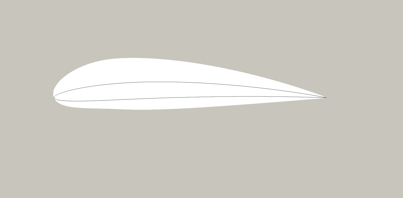
Figure 1: Two airfoils superimposed.

3.1.2 Training

After performing the dimensionality reduction step, we train two Gaussian processes regression models [33] as follows.

1. The first model is to learn the optimal mapping that transforms the reference configuration to the optimal configuration. This model takes as input the physical parameter $\mu_{i}$ and the geometrical mapping POD coefficient $\alpha_{i}$, and as output the optimal mapping POD coefficient $\beta_{i}$. We denote this model by $\mathcal{R}:\mathbb{R}^{p}\times\mathbb{R}^{q}\to\mathbb{R}^{t}$.

2. The second model is to learn the field in the optimal configuration. This model takes as input the physical parameter $\mu_{i}$ and the geometrical mapping POD coefficient $\alpha_{i}$, and as output the field in the optimal configuration POD coefficient $\gamma_{i}$. We denote this model by $\mathcal{O}:\mathbb{R}^{p}\times\mathbb{R}^{q}\to\mathbb{R}^{r}$.

3.2 Inference phase

In the inference phase, we are given a new unseen geometry $\widetilde{\Omega}$ in the inference phase, with a physical parameter $\widetilde{\mu}$. The goal is to predict the field of interest $\widetilde{u}$, solution to the physical simulation. We proceed in the following manner.

1. First, we compute the geometrical mapping $\widetilde{\bm{\phi}}^{\rm geo}$ that maps $\Omega_{0}$ onto $\widetilde{\Omega}$, then we project $\widetilde{\bm{\phi}}^{\rm geo}-\bm{Id}$ on the POD basis $\{\bm{\zeta}^{\rm geo}_{i}\}_{1\leq i\leq n}$ to obtain the coefficient $\widetilde{\alpha}$.

2. We use the pair $(\widetilde{\alpha},\widetilde{\mu})$ to infer $\widetilde{\beta}=\mathcal{R}(\widetilde{\alpha},\widetilde{\mu})$ and $\widetilde{\gamma}=\mathcal{O}(\widetilde{\alpha},\widetilde{\mu})$. We obtain $\displaystyle\widetilde{\bm{\phi}}^{\rm opt}:=\bm{Id}+\sum_{j=1}^{t}\widetilde{\beta}_{j}\bm{\zeta}^{\rm opt}_{j}$ and $\displaystyle\widetilde{u}^{\rm opt}:=\sum_{j=1}^{r}\widetilde{\gamma}_{j}\psi_{j}$.

3. Finally, the quantity of interest $\widetilde{u}$ is obtained as

   $$\widetilde{u}:=\widetilde{u}^{\rm opt}\circ\left(\widetilde{\bm{\phi}}^{\rm opt}\right)^{-1}\circ\left(\widetilde{\bm{\phi}}^{\rm geo}\right)^{-1}.$$

4 Geometrical mapping

Numerous techniques exists in the literature to construct a mapping between domains [2, 4, 31]. In this work, we use RBF morphing [10] to construct the mapping from the reference domain $\Omega_{0}$ to each target domain $\Omega_{i}$. When using this technique, we suppose that the deformation on a subset of points in $\Omega_{0}$, called the control points, is known. These points are usually on the boundary of $\Omega_{0}$. Then, we can leverage the knowledge of $\bm{\phi}_{i}(\partial\Omega_{0})=\partial\Omega_{i}$ to compute the deformation in the bulk of the domain $\bm{\phi}_{i}(\Omega_{0})$. In this work, we suppose that the geometries are not parametrized and $\bm{\phi}_{i}(\partial\Omega_{0})$ is not given. Thus, we start by computing $\bm{\phi}_{i}(\partial\Omega_{0})$, for all $1\leq i\leq n$, which is case dependent in this work. When computing $\bm{\phi}_{i}(\partial\Omega_{0})$ is not available, methods as proposed in [11, 15] provides solutions to automatically finds a mapping from the reference onto the target domain. We refer to appendix D for a brief discussion on the RBF morphing method.

5 Optimal mapping

The second major building block we introduce is the optimal mapping algorithm to compute $\Phi^{\rm opt}=(\bm{\phi}^{\rm opt}_{i})_{1\leq i\leq n}$ that maximize the energy in the first $r$ modes.

In order to pass from the reference configuration to the optimal configuration, we solve (3):

$$\text{find }\Phi^{*}\in\arg\max_{\Phi\in\mathbf{M}_{0}^{n}}J_{\mathcal{U},r}[\Phi].$$

The optimization problem presented here is non-convex with possibly infinitely many solutions. We present here briefly the optimization strategy employed to solve this problem. Refer to the appendixes for a detailed discussion.

5.1 Gradient algorithm in infinite dimension

We can show that the differential of $J_{\mathcal{U},r}$ with respect to $\Phi$ at a point $\Psi$ has the following expression (see appendix A):

$$DJ_{\mathcal{U},r}[\Phi][\Psi]=\sum_{i=1}^{n}\int_{\Omega_{0}}\mathbf{f}_{i}[\Phi]\cdot\bm{\psi}_{i}dx.$$

with

$$\mathbf{f}_{i}[\Phi]:=\sum_{j=1}^{n}\theta_{ij}u_{j}^{\rm ref}\circ\bm{\phi}_{j}\vec{\nabla}u_{i}^{\rm ref}\circ\bm{\phi}_{i},$$ (4)

and $\displaystyle\theta_{ij}:=\sum_{k=1}^{r}\left(\frac{2\zeta^{\mathcal{U}}_{k,i}[\Phi]\zeta^{\mathcal{U}}_{k,j}[\Phi]}{Tr(C_{\mathcal{U}}[\Phi])}-\frac{\displaystyle 2\lambda_{k}^{\mathcal{U}}[\Phi]}{Tr(C_{\mathcal{U}}[\Phi])^{2}}\delta_{ij}\right)$.
A standard gradient algorithm in infinite dimension consists of (i) choosing an appropriate inner product, denoted here by $a$, (ii) computing the Riesz representation of each $\mathbf{f}_{i}[\Phi]$ with respect to $a$, which will be denoted by $\bm{u}_{i}[\Phi]$ and finally (iii) updating, at each iteration $m$, $\bm{\phi}_{i}^{(m)}$ by

$$\bm{\phi}_{i}^{(m+1)}=\bm{\phi}_{i}^{(m)}+\epsilon\bm{u}_{i}[\Phi^{(m)}]$$ (5)

with $\epsilon>0$ in the gradient step. The simplest example of $a$ is the $L_{2}(\Omega_{0})$ inner product which gives the following iterative scheme:

$$\bm{\phi}_{i}^{(m+1)}=\bm{\phi}_{i}^{(m)}+\epsilon\mathbf{f}_{i}[\Phi^{(m)}].$$ (6)

However, this may suffer from one of the following problems:

• $\bm{\phi}_{i}^{(m+1)}$ might not be bijective.

• $\bm{\phi}_{i}^{(m+1)}$ might not map $\Omega_{0}$ onto itself.

• If the function $\Phi^{(m)}$ is far from a maximum, the algorithm may fail to converge properly.

We address these issues in the following subsections.

5.2 Bijectivity

To address bijectivity, we consider the following optimization statement:

$$\text{find }\Phi^{*}\in\arg\max_{\Phi\in\mathbf{M}^{n}_{0}}I_{\mathcal{U},r}[\Phi]:=J_{\mathcal{U},r}[\Phi]-c_{1}\sum_{i=1}^{n}E[\bm{\phi}_{i}],$$ (7)

where $E$ is an energy term to enforce bijectivity and $c_{1}>0$ is a penalization parameter. Ideally, the term $E$ should diverge to $+\infty$ if the mapping $\bm{\phi}_{i}$ becomes non-bijective. In this case, the objective function $I$ diverges to $-\infty$. One example for the energy term is the elastic energy for non-linear Neohookean model. In this work, we use linear elastic energy for the term $E$, (we note that it does not diverges to $+\infty$ for non-bijective mappings, however, it gives acceptable results). Finally, we solve the problem 7 using the continuation method, which consists of iteratively decrease the parameter $c_{1}$ in order to obtain a solution to problem 3. We give more details about the continuation method and the term $E$ in appendix C.

5.3 Mapping condition

To guarantee that $\bm{\phi}_{i}$ always maps $\Omega_{0}$ onto itself, we partition the boundary of $\Omega_{0}$ to $\partial\Omega_{0}:=\partial\Omega_{0}^{p}\bigcup\partial\Omega_{0}^{c}$ with $\partial\Omega_{0}^{p}$ is the union of all the faces (edges in $2d$) of $\partial\Omega_{0}$ and $\partial\Omega_{0}^{c}$ is the curved part of $\partial\Omega_{0}$. We define the space $H_{\bm{n}}^{1}(\Omega_{0}):=\{\bm{u}\in H^{1}(\Omega_{0}):\bm{u}\cdot\bm{n}=0\text{ on }\partial\Omega_{0}^{p},\bm{u}=0\text{ on }\partial\Omega_{0}^{c}\}$

and the inner product $a$ on $H_{\bm{n}}^{1}(\Omega_{0})$ as

$$(\bm{u},\bm{v})\mapsto a(\bm{u},\bm{v}):=\int_{\Omega_{0}}\sigma(\bm{u}):\varepsilon(\bm{v})d\mathbf{x},$$ (8)

with $\sigma$ and $\varepsilon$ are respectively the elasticity stress and strain tensors. We compute, for all $1\leq i\leq n$, and for each iteration $m$, the Riesz representation $\bm{u}_{i}^{(m)}$ of $\mathbf{f}_{i}$ with respect to this inner product, which is the unique solution to

$$\forall\bm{v}\in H_{\bm{n}}^{1}({\Omega_{0};{\mathbb{R}}^{d}}),\quad a(\bm{u}_{i}^{(m)},\bm{v})=\int_{\Omega_{0}}\mathbf{f}_{i}[\Phi^{(m)}]\bm{v}d\mathbf{x},$$ (9)

to obtain the iterative scheme:

$$\bm{\phi}_{i}^{(m+1)}=\bm{\phi}_{i}^{(m)}+\epsilon\bm{u}_{i}[\Phi^{(m)}].$$ (10)

We can also obtain a similar expression when solving problem $\eqref{eq: I definition}$ and using linear elastic energy (see more in appendix C):

$$\bm{\phi}^{(m+1)}_{i}=\bm{\phi}^{(m)}_{i}+\epsilon\left(\bm{u}_{i}[\Phi^{(m)}]-c_{1}\left(\bm{\phi}_{i}^{(m)}-Id\right)\right).$$ (11)

By using the above procedure, we guarantee that, if $\bm{\phi}_{i}^{(m)}+\epsilon\bm{u}_{i}[\Phi^{(m)}]$ is bijective, then necessary we have that the points on $\partial\Omega_{0}^{p}$ stay on $\partial\Omega_{0}^{p}$, as they are only allowed to move tangentially, while points on $\partial\Omega_{0}^{c}$ stay fixed. Thus, $\bm{\phi}_{i}^{(m)}+\epsilon\bm{u}_{i}[\Phi^{(m)}]$ preserves the boundary of $\Omega_{0}$. We note however that this is suboptimal as we do not allow $\partial\Omega_{0}^{c}$ to deform in this case. A full treatment of curved boundaries is the subject of future work. One possible solution would be to always choose the reference domain $\Omega_{0}$ to be a polytope (thus $\partial\Omega_{0}=\partial\Omega_{0}^{p}$) .

5.4 Uncorrelated samples

One major reason for the poor convergence of the gradient algorithm is when the samples are heavily not correlated. This happens when the non-zero values of $u_{i}^{\rm ref}$ are compactly supported in $\Omega_{0}$. More precisely, if, for some $1\leq j\leq n$, $\rm{supp}$$(u_{j}^{\rm ref}\circ\bm{\phi}_{j})\bigcap\rm{supp}$$(\vec{\nabla}u_{i}^{\rm ref}\circ\bm{\phi}_{i})=\emptyset$, then the contribution of $u_{j}^{\rm ref}\circ\bm{\phi}_{j}\vec{\nabla}u_{i}^{\rm ref}\circ\bm{\phi}_{i}$ in $\mathbf{f}_{i}$ is null. To this end, we transform the fields $\{u_{i}\}_{1\leq i\leq n}$ to the family of fields $\widehat{\mathcal{U}}(c_{2}):=\{\widehat{u}_{i}\}_{1\leq i\leq n}$, where each is defined as the solution to

$$- \Delta\widehat{u}_{i}+c_{2}\widehat{u}_{i}=c_{2}u_{i},$$ (12)

$$\partial_{n}\widehat{u}_{i}=0$$

where $\Delta$ is the Laplacian operator and $c_{2}>0$. This equation has a unique solution. The transformed fields will diffuse the value of $u_{i}$ throughout the domain $\Omega_{0}$ for small values of $c_{2}$ (see Figures 3-4). On the other hand, $\widehat{u}_{i}$ converges to $u_{i}$ as $c_{2}$ goes to $+\infty$. We use the fields $\widehat{\mathcal{U}}(c_{2})$ in order to solve (3)-(7). The value of $c_{2}$ is also changed throughout the iterations using the continuation method.

6 Numerical examples

In this section, we illustrate the method on two examples of non-reducible problems.

6.1 Example 1: advection-reaction equation

This example is taken from [30], and it illustrates a non-reducible problem. Here, we show the effect of the optimal mapping algorithm on a fixed geometry. Let the following advection-reaction equation:

$$\begin{cases}\nabla\cdot(c_{\mu}u_{\mu})+\sigma_{\mu}u_{\mu}=f_{\mu}&\text{in }\Omega=(0,1)^{2},\\ u_{\mu}=u_{D,\mu}&\text{on }\Gamma_{\text{in},\mu}:=\{x\in\partial\Omega:c_{\mu}\cdot\bm{n}<0\},\end{cases}$$

where $\bm{n}$ denotes the outward normal to $\partial\Omega$, and

$$c_{\mu}=\begin{bmatrix}\cos(\mu_{1})\\ \sin(\mu_{1})\end{bmatrix},\quad\sigma_{\mu}=1+\mu_{2}e^{x_{1}+x_{2}},\quad f_{\mu}=1+x_{1}x_{2},$$

$$u_{D,\mu}=4\arctan\left(\mu_{3}\left(x_{2}-\frac{1}{2}\right)\right)(x_{2}-x_{2}^{2}),$$

$$\mu=[\mu_{1},\mu_{2},\mu_{3}]\in\mathcal{P}:=\left[-\frac{\pi}{10},\frac{\pi}{10}\right]\times[0.3,0.7]\times[60,100].$$

We consider $n=250$ samples. In Figure 2, we plot $u_{\mu}$ for three different values of the parameter before and after computing the optimal mappings that maximize $J_{\mathcal{U},r}$, for $r=1$. We can clearly see how the optimal mappings will align automatically the discontinuities in the samples.

Figure 2: Top: three samples before the optimization. Bottom: three samples after the optimization.

The optimal mappings algorithm can be seen as a multi-modal generalization to the registration methods, where the case $r=1$ gives similar results to aligning all the samples on one mode. However, the advantage of our method is that we can go beyond a single mode.

6.2 Example 2: ML4CFD NeurIPS 2024 competition

In the second example, we apply the method to the airfoil design case considered in the ML4CFD NeurIPS 2024 competition [34], and we compare it with the winning solution. The dataset adopted for the competition is the AirfRANS dataset from [6]. Each sample have two scaler inputs, the inlet velocity and the angle of attack, and three output fields, the velocity, pressure and the turbulent viscosity. The dataset is composed of three splits.

1. Training set: composed of 103 samples.

2. Testing set: composed of 200 samples.

3. OOD testing set: composed of 496 samples, where the Reynold number considered for samples in this split is taken out of distribution.

In this work, we focus on the turbulent viscosity field as it represents a non-reducible field. We illustrate this field in Figure 3.

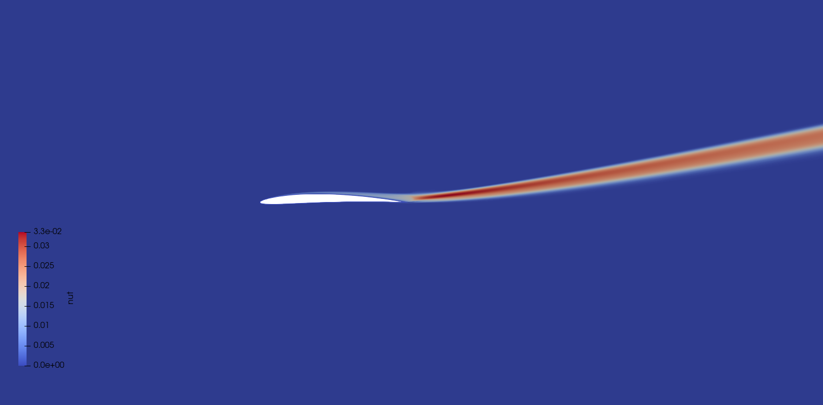
Figure 3: The turbulent viscosity field illustrated for two of the samples.

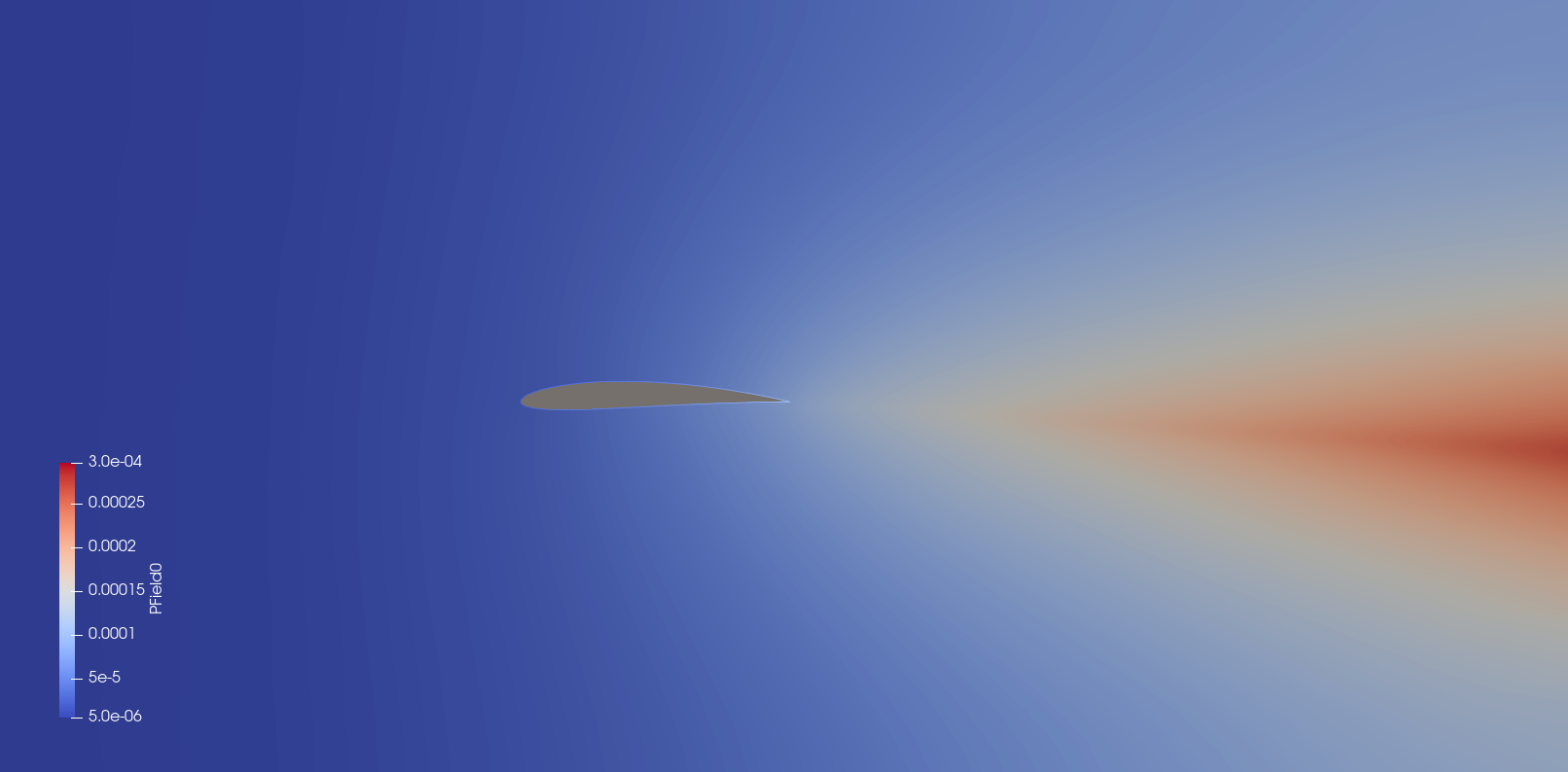
Figure 4: The diffused field $\widehat{u}$ for $c_{2}=1$ .

6.2.1 MMGP: mesh morphing Gaussian process

The method we present in this paper is founded on the MMGP method [8]. The main differences being:

1. First, in MMGP, the mapping $\phi_{i}^{\rm geo}$ is computed from each geometry onto the reference domain $\Omega_{0}$. In this case, the input to the GP model is the POD coefficients of the inverse mapping $(\phi_{i}^{\rm geo})^{-1}$. Thus, evaluating $(\phi_{i}^{\rm geo})^{-1}$ would introduce extra computations to the procedure. In addition, when using RBF morphing, such as in this work, computing $\phi_{i}^{\rm geo}$ from the same geometry proves to be much efficient numerically, as the RBF interpolation matrix $\mathbf{K}$ can be assembled and factorized once and for all (see appendix D for the definition of $\mathbf{K}$).

2. Secondly, the MMGP mappings are not field-optimized. This is equivalent to omitting the transition to the optimal configuration. So, when it comes to non-reducible problems, even if a large number of modes are retained, the error introduced by POD truncation and the discretization error would remain large to obtain reliable predictions for new samples.

6.2.2 NeurIPS solution: MMGP + wake line prediction

The winning solution to the ML4CFD competition [7] relies on the application of MMGP, with the addition of aligning the wake line behind the airfoil for all the samples at same position. The latter step being necessary to obtain accurate prediction of the turbulent viscosity. While this correction step gives accurate results, it remains case-dependent and needs to be done manually. Moreover, it suffers from the same problem as any other registration technique, which is the restriction to one mode.

6.2.3 O-MMGP: optimal mesh morphing Gaussian process

We run the optimal mapping algorithm in order to maximize the compression of the turbulent viscosity field. We choose the reference geometry $\Omega_{0}$ to be one of the samples in the training set. We then proceed to compute $\phi_{i}^{\rm geo}$ using RBF morphing. Once computed, we solve problem 7 for the family $\widehat{\mathcal{U}}(c_{2})$. We choose $r:=1$, $c_{1}^{(0)}:=0.1$ and $c_{2}^{(0)}:=1$. The last two parameters are changed throughout the iterations as mentioned in appendix C. In Figure 5, we show that the eigenvalues of the correlation matrix of $(\bm{\phi}_{i}^{\rm opt})_{1\leq i\leq n}$ decay rapidly, proving numerically that this family is reducible, and justifying the regression on the optimal mapping POD coordinates.

Figure 5: Decay of the eigenvalues of the correlation matrix of the family $(\bm{\phi}_{i}^{\rm opt})_{1\leq i\leq n}$ .

After computing the optimal mappings, we train two Gaussian process regression models, one to learn the optimal mapping $\widetilde{\bm{\phi}}$, and the other to learn the field $\widetilde{u}$, which is the turbulent viscosity in this case.

In order to show the efficiency of the method, we compare the results of the following three tests:

1. First, we apply the method without solving the optimal mappings problem, similar to the original MMGP method. Thus, we predict the turbulent viscosity field in the reference configuration.

2. Second, we run the winning solution of the NeurIPS 2024 challenge, aligning the wake line behind the airfoil manually.

3. Finally, we apply the full O-MMGP procedure described in this paper.

In table 1, we report the mean square error (MSE) of the three tests on the turbulent viscosity field, for the testing and OOD splits. While the original MMGP performs poorly for this field, the O-MMGP method produces very accurate predictions, slightly surpassing the NeurIPS 2024 competition solution. The major advantage of the method is that the alignment of the snapshot was done automatically, without using the specificity of the case.

	MMGP	NeurIPS solution	O-MMGP
Test	0.143	0.025	0.024
OOD	0.171	0.048	0.046

Table 1: MSE errors for the different tests.

In Figure 6, we report the decay of the eigenvalues of the correlation matrix for the three tests. For the MMGP solution, no aligning of the solution was performed, which explains the slow decay of the eigenvalues for this case. As expected, the eigenvalues decays the most rapidly when using the optimal mappings algorithm.

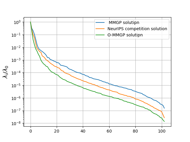
Figure 6: Decay of the eigenvalues of the correlation matrix for the turbulent viscosity fields in the three tests.

7 Conclusion

In this article, we have presented a new algorithm that aims to maximize the energy in the first $r$ principal modes of a family of functions. The novelty of the algorithm lies in the fact that it automatically aligns the functions on an arbitrary number of modes, unlike other methods in the literature which may require feature tracking of the solution or assume that the family of functions can be compressed onto a single mode. We have shown how the proposed method can be integrated into the MMGP workflow to learn and predict the solutions of PDEs with geometric variabilities. The quality of the prediction was found to be on a par with state-of-the-art methods. Current work aims to solve the problem in the general case of curved boundaries and provide a more thorough mathematical analysis of the method, as well as applying the method in the presence of multiple shocks.

Appendix

Appendix A Differential of $J_{\mathcal{H},r}$

Let $\Phi=(\bm{\phi}_{i})_{1\leq i\leq n}\in\mathbf{M}$, $\Psi=(\bm{\psi}_{i})_{1\leq i\leq n}$ a "small" variation around $\Phi$ and $\epsilon\in{\mathbb{R}},\epsilon<<1$. To evaluate the differential of $J_{\mathcal{H},r}$ at a point $\Phi$, we evaluate $J_{\mathcal{H},r}$ at $\bar{\Phi}:=\Phi+\epsilon\Psi$ and calculate:

$$DJ_{\mathcal{H},r}[\Phi][\Psi]=\lim_{\epsilon\to 0}\displaystyle\frac{J_{\mathcal{H},r}(\Phi+\epsilon\Psi)-J_{\mathcal{H},r}(\Phi)}{\epsilon}$$ (13)

We have:

$$\forall i,\hskip 5.0pth_{i}\circ(\bm{\phi}_{i}+\epsilon\bm{\psi}_{i})(x) =h_{i}(\bm{\phi}_{i}(x)+\epsilon\bm{\psi}_{i}(x))$$

$$\simeq h_{i}(\bm{\phi}_{i}(x))+\epsilon\vec{\nabla}h_{i}(\bm{\phi}_{i}(x))\cdot\bm{\psi}_{i}(x)$$

where we neglect higher order terms. Next we evaluate :

$$\displaystyle C_{\mathcal{H},ij}[\Phi+\epsilon\Psi] =\langle h_{i}\circ(\bm{\phi}_{i}+\epsilon\bm{\psi}_{i}),h_{j}\circ(\bm{\phi}_{j}+\epsilon\bm{\psi}_{j})\rangle_{L^{2}(\Omega_{0})}$$

$$=\int_{\Omega_{0}}h_{i}\circ(\bm{\phi}_{i}+\epsilon\bm{\psi}_{i})(x)h_{j}\circ(\bm{\phi}_{j}+\epsilon\bm{\psi}_{j})(x)dx$$

$$=\int_{\Omega_{0}}h_{i}\circ\bm{\phi}_{i}(x)h_{j}\circ\bm{\phi}_{j}(x)dx+\epsilon\int_{\Omega_{0}}h_{i}\circ\bm{\phi}_{i}(x)\vec{\nabla}h_{j}(\bm{\phi}_{j}(x))\cdot\bm{\psi}_{j}(x)dx$$ (14)

$$+\epsilon\int_{\Omega_{0}}\vec{\nabla}h_{i}(\bm{\phi}_{i}(x))\cdot\bm{\psi}_{i}(x)h_{j}\circ\bm{\phi}_{j}(x)dx+\epsilon^{2}\int_{\Omega_{0}}\vec{\nabla}h_{i}(\bm{\phi}_{i}(x))\bm{\psi}_{i}(x)\vec{\nabla}h_{j}(\bm{\phi}_{j}(x))\bm{\psi}_{j}(x)dx$$

$$:=C_{\mathcal{H},ij}[\Phi]+\epsilon DC_{\mathcal{H},ij}[\Phi][\Psi]+\epsilon^{2}D^{2}C_{\mathcal{H},ij}[\Phi][\Psi]$$

and

$$Tr(C_{\mathcal{H}}[\Phi+\epsilon\Psi]) =\sum C_{ii}[\Phi+\epsilon\Psi]$$

$$=Tr(C_{\mathcal{H}}[\Phi])+2\epsilon\sum_{i=1}^{n}\int_{\Omega_{0}}h_{i}\circ\bm{\phi}_{i}(x)\vec{\nabla}h_{i}(\bm{\phi}_{i}(x))\cdot\bm{\psi}_{i}(x)dx+\epsilon^{2}\sum_{i=1}^{n}\int_{\Omega_{0}}[\vec{\nabla}h_{i}(\bm{\phi}_{i}(x))\cdot\bm{\psi}_{i}(x)]^{2}dx$$

$$=Tr(C_{\mathcal{H}}[\Phi])+\epsilon Tr(DC_{\mathcal{H}}[\Phi][\Psi])+\epsilon^{2}D^{2}C_{\mathcal{H}}[\Phi][\Psi]$$

with $DC_{\mathcal{H},ij}[\Phi][\Psi]:=\displaystyle\int_{\Omega_{0}}h_{i}\circ\bm{\phi}_{i}(x)\vec{\nabla}h_{j}(\bm{\phi}_{j}(x))\cdot\bm{\psi}_{j}(x)dx+\int_{\Omega_{0}}\vec{\nabla}h_{i}(\bm{\phi}_{i}(x))\cdot\bm{\psi}_{i}(x)h_{j}\circ\bm{\phi}_{j}(x)dx$ and $DC_{\mathcal{H}}[\Phi][\Psi]=(DC_{\mathcal{H},ij}[\Phi][\Psi])_{1\leq i,j\leq n}$.

Next we evaluate $D\lambda_{i}^{\mathcal{H}}[\Phi][\Psi]$. We have $\forall i$ :

$$||\zeta_{i}^{\mathcal{H}}[\Phi]||^{2}=1$$

Now taking the differential on both sides, we get

$$\langle D\zeta_{i}^{\mathcal{H}}[\Phi][\Psi],\zeta_{i}^{\mathcal{H}}[\Phi]\rangle=0$$

Using the fact that $C_{\mathcal{H}}[\Phi]\zeta_{i}^{\mathcal{H}}[\Phi]=\lambda_{i}^{\mathcal{H}}[\Phi]\zeta_{i}^{\mathcal{H}}[\Phi]$, we get again by taking the differential on both sides

$$DC_{\mathcal{H}}[\Phi][\Psi]\zeta_{i}^{\mathcal{H}}[\Phi]+C_{\mathcal{H}}[\Phi]D\zeta_{i}^{\mathcal{H}}[\Phi][\Psi]=D\lambda_{i}^{\mathcal{H}}[\Phi][\Psi]\zeta_{i}^{\mathcal{H}}[\Phi]+\lambda_{i}^{\mathcal{H}}[\Phi]D\zeta_{i}^{\mathcal{H}}[\Phi][\Psi]$$

We multiply the last equation by $\zeta_{i}^{\mathcal{H}}[\Phi]$ to get

$$(\zeta_{i}^{\mathcal{H}}[\Phi])^{T}DC_{\mathcal{H}}[\Phi][\Psi]\zeta_{i}^{\mathcal{H}}[\Phi]+0=D\lambda_{i}^{\mathcal{H}}[\Phi][\Psi]+0$$

Thus we have finally

$$\lambda_{i}^{\mathcal{H}}[\Phi+\epsilon\Psi]=\lambda_{i}^{\mathcal{H}}[\Phi]+(\zeta_{i}^{\mathcal{H}}[\Phi])^{T}DC_{\mathcal{H}}[\Phi][\Psi]\zeta_{i}^{\mathcal{H}}[\Phi]\hskip 10.00002pt,\forall 1\leq i\leq n$$ (15)

Taking the sum over the first $r$ eigenvalues, we obtain:

$$\displaystyle\sum_{j=1}^{r}\lambda_{j}^{\mathcal{H}}[\Phi+\epsilon\Psi]=\displaystyle\sum_{j=1}^{r}\lambda_{i}^{\mathcal{H}}[\Phi][\Psi]+\epsilon Tr((\mathrm{Z}^{\Phi}_{r})^{T}DC_{\mathcal{H}}[\Phi][\Psi]\mathrm{Z}^{\Phi}_{r})$$ (16)

with $\mathrm{Z}^{\Phi}_{r}=(\zeta_{1}^{\Phi},\zeta_{2}^{\Phi},\cdots,\zeta_{r}^{\Phi})^{T}$. Now we can evaluate (13) to obtain:

$$DJ_{\mathcal{H},r}[\Phi][\Psi]=\frac{Tr((\mathrm{Z}^{\Phi}_{r})^{T}DC_{\mathcal{H}}[\Phi][\Psi]\mathrm{Z}^{\Phi}_{r})}{Tr(C_{\mathcal{H}}[\Phi])}-\frac{\displaystyle\sum_{k=1}^{r}\lambda_{k}^{\mathcal{H}}[\Phi]}{Tr(C_{\mathcal{H}}[\Phi])^{2}}\times Tr(DC_{\mathcal{H}}[\Phi][\Psi])$$ (17)

which can be written explicitly as

$$DJ_{\mathcal{H},r}[\Phi][\Psi] =\frac{2}{Tr(C_{\mathcal{H}}[\Phi])}\sum_{i=1}^{n}\sum_{j=1}^{n}\sum_{k=1}^{r}\zeta^{\mathcal{H}}_{k,i}[\Phi]\zeta^{\mathcal{H}}_{k,j}[\Phi]\displaystyle\int_{\Omega_{0}}h_{j}\circ\bm{\phi}_{j}(x)\vec{\nabla}h_{i}(\bm{\phi}_{i}(x))\cdot\bm{\psi}_{i}(x)dx$$

$$-\frac{\displaystyle 2\sum_{k=1}^{r}\lambda_{k}^{\mathcal{H}}[\Phi]}{Tr(C_{\mathcal{H}}[\Phi])^{2}}\sum_{i=1}^{n}\int_{\Omega_{0}}h_{j}\circ\bm{\phi}_{j}(x)\vec{\nabla}h_{i}(\bm{\phi}_{i}(x))\cdot\bm{\psi}_{i}(x)dx$$

$$=\sum_{i=1}^{n}DJ_{i}[\Phi][\bm{\psi}_{i}]$$

with

$$DJ_{i}[\Phi][\bm{\psi}_{i}] :=\sum_{k=1}^{r}\Big{(}\frac{2{\zeta^{\mathcal{H}}_{k,i}[\Phi]}^{2}}{Tr(C_{\mathcal{H}}[\Phi])}-\frac{\displaystyle 2\lambda_{k}^{\mathcal{H}}[\Phi]}{Tr(C_{\mathcal{H}}[\Phi])^{2}}\Big{)}\int_{\Omega_{0}}h_{i}\circ\bm{\phi}_{i}(x)\vec{\nabla}h_{i}(\bm{\phi}_{i}(x))\cdot\bm{\psi}_{i}(x)dx$$

$$+\sum_{j=1\atop j\neq i}^{n}\sum_{k=1}^{r}\frac{2\zeta^{\mathcal{H}}_{k,i}[\Phi]\zeta^{\mathcal{H}}_{k,j}[\Phi]}{Tr(C_{\mathcal{H}}[\Phi])}\int_{\Omega_{0}}h_{j}\circ\bm{\phi}_{j}(x)\vec{\nabla}h_{i}(\bm{\phi}_{i}(x))\cdot\bm{\psi}_{i}(x)dx$$

$$=\sum_{j=1}^{n}\sum_{k=1}^{r}\left(\frac{2\zeta^{\mathcal{H}}_{k,i}[\Phi]\zeta^{\mathcal{H}}_{k,j}[\Phi]}{Tr(C_{\mathcal{H}}[\Phi])}-\frac{\displaystyle 2\lambda_{k}^{\mathcal{H}}[\Phi]}{Tr(C_{\mathcal{H}}[\Phi])^{2}}\delta_{ij}\right)\int_{\Omega_{0}}h_{j}\circ\bm{\phi}_{j}(x)\vec{\nabla}h_{i}(\bm{\phi}_{i}(x))\cdot\bm{\psi}_{i}(x)dx,$$ (18)

and $\delta_{ij}$ is the Kronecker delta. For simplicity, we note the term

$$\mathbf{f}_{i}[\Phi]:=\sum_{j=1}^{n}\sum_{k=1}^{r}\left(\frac{2\zeta^{\mathcal{H}}_{k,i}[\Phi]\zeta^{\mathcal{H}}_{k,j}[\Phi]}{Tr(C_{\mathcal{H}}[\Phi])}-\frac{\displaystyle 2\lambda_{k}^{\mathcal{H}}[\Phi]}{Tr(C_{\mathcal{H}}[\Phi])^{2}}\delta_{ij}\right)h_{j}\circ\bm{\phi}_{j}(x)\vec{\nabla}h_{i}(\bm{\phi}_{i}(x)),$$ (19)

$\mathbf{F}[\Phi]:=(\mathbf{f}_{1}[\Phi],\cdots,\mathbf{f}_{n}[\Phi])$, and we write

$$DJ_{\mathcal{H},r}[\Phi][\Psi]=\sum_{i=1}^{n}\int_{\Omega_{0}}\mathbf{f}_{i}[\Phi]\cdot\bm{\psi}_{i}dx.$$

Appendix B Differential of $I_{\mathcal{H},r}$

We define the objective function $I_{\mathcal{H},r}$ on $\mathrm{M}_{0}^{n}$ as

$$I_{\mathcal{H},r}[\Phi]:=J_{\mathcal{H},r}[\Phi]-c_{1}\sum_{i=1}^{n}E[\bm{\phi}_{i}].$$

As mentioned in section 5, the energy term used in this work in the linear elastic energy defined as

$$E[\bm{\phi}_{i}]:=\frac{1}{2}a(\bm{\phi}_{i}-\bm{Id},\bm{\phi}_{i}-\bm{Id}),$$

where we recall the definition of $a$ in (8). We can easily show that

$$DE[\bm{\phi}_{i}][\bm{\psi}]=a(\bm{\phi}_{i}-\bm{Id},\bm{\psi}).$$

Using the linearity of the differential, we obtain the differential of $I_{\mathcal{H},r}$ as

$$DI_{\mathcal{H},r}[\Phi][\Psi] =DJ[\Phi][\Psi]-c_{1}\sum_{i=1}^{n}DE[\bm{\phi}_{i}][\bm{\psi}_{i}]$$

$$=\sum_{i=1}^{n}\int_{\Omega_{0}}\mathbf{f}_{i}[\Phi]\cdot\bm{\psi}_{i}dx-c_{1}\sum_{i=1}^{n}DE[\bm{\phi}_{i}][\bm{\psi}_{i}]$$

$$=\sum_{i=1}^{n}\left(\int_{\Omega_{0}}\mathbf{f}_{i}[\Phi]\cdot\bm{\psi}_{i}dx-c_{1}DE[\bm{\phi}_{i}][\bm{\psi}_{i}]\right)$$

$$:=\sum_{i=1}^{n}DI_{i}[\Phi][\bm{\psi}_{i}].$$

In order to obtain equation (11), we compute the Riesz representation of $DI_{i}[\Phi]$, denoted as $\bar{\bm{u}}$, with respect to the inner product $a$, the unique solution to

$$a(\bar{\bm{u}}_{i},\bm{\psi})=\int_{\Omega_{0}}\mathbf{f}_{i}[\Phi]\cdot\bm{\psi}_{i}dx-c_{1}a(\bm{\phi}_{i}-\bm{Id},\bm{\psi}),$$

for all test function $\bm{\psi}$. Since we also have $\bm{u}_{i}$ as the Riesz representation of $DJ_{i}[\Phi]$ $\left(a(\bm{u}_{i},\bm{\psi})=DJ_{i}[\Phi][\bm{\psi}]\right)$, we obtain

$$a(\bar{\bm{u}}_{i},\bm{\psi})=a(\bm{u}_{i},\bm{\psi})-c_{1}a(\bm{\phi}_{i}-\bm{Id},\bm{\psi}).$$

which is true for all test function $\bm{\psi}$. Thus, by the linearity of $a$, we obtain $\bar{\bm{u}}_{i}=\bm{u}_{i}-c_{1}(\bm{\phi}_{i}-\bm{Id})$, and hence equation (11).

Appendix C Continuation method

We give here a quick description on the continuation methods. Readers can refer to [1, 27] and references within for more details.

Continuation methods are a variety of methods used to solve equations of the type

$$G(x)=0$$

where $G$ is a non-linear function, and $x$ is the unknown. Continuation methods rely on solving a succession of problems of the form

$$H(x,\lambda)=0$$

where $H$ is another non-linear function and $H(x,\lambda^{*})=G(x)$ for some $\lambda^{*}$. $\lambda$ is called the continuation parameter. In the simplest form of a continuation method, we start by choosing a set a values $\{\lambda^{0},\lambda^{1}\cdots\lambda^{*}\}$ for $\lambda$. We then solve $H(x^{i},\lambda^{i})=0$, and initialize $H(x^{i+1},\lambda^{i+1})=0$ with $x^{i}$.

C.1 Continuation for $c_{1}$

In order to solve equation (7), we proceed by using the continuation method as follows:

1. We start by solving equation the optimization problem, using the gradient algorithm, for $c_{1}=c_{1}^{0}$, where $c_{1}^{0}$ should be sufficiently large in order to converge properly. This will produce the function $\Phi^{0}$.

2. At each iteration $k$, we set $\displaystyle c_{1}^{k}:=\frac{c_{1}^{k-1}}{2}$, and we resolve the problem for $\Phi^{k}$ by initializing $\Phi^{(0),k}=\Phi^{k-1}$ .

3. We iterate over $k$ as long as there are no elements of the morphed meshes are inverted.

We give a few comments about the above procedure. First, we note that there are two loops for the algorithm: the outer loop over $k$ that updates $c_{1}$, and the inner loop that solves the non-linear equation using the gradient algorithm. Second, ideally we want to solve (7) for $c_{1}=0$. If, while iterating over the outer loop, $c_{1}^{k}$ gets sufficiently small, we can set $c_{1}^{k+1}=0$. Finally, we note that full convergence for intermediate results of $\Phi^{k}$ is generally not necessary.

C.2 Continuation for $c_{2}$

Applying continuation with two or more parameters proves to be more complicated for the case of one parameter. To this end, we propose in this paper to alternate changing the values of the two parameters $c_{1}$ and $c_{2}$. We proceed in the same manner as above, expect that:

1. At iteration $2k$, we set $c_{1}^{2k}:=\frac{c_{1}^{2k-1}}{2}$.

2. We start with a small value for $c_{2}^{0}$. At iteration $2k+1$, we set $c_{2}^{2k+1}:=10\times c_{2}^{2k}$.

Appendix D RBF morphing

In radial basis function (RBF) interpolation, we aim to approximate a scalar-valued function $g(x)$ using a linear combination of radial basis functions as follows:

$$g(x)\approx\sum_{i=1}^{n_{c}}a_{i}\,\xi(\|x-x_{i}\|),$$ (20)

where $a_{i}\in{\mathbb{R}}$ and $\xi$ is a radial basis function that depends only on the Euclidean distance between $x$ and a control point $x_{i}$. The control points $\{x_{i}\mid i=1,\ldots,n_{c}\}$ are specific locations where the exact values of $g(x)$, denoted $g_{i}$, are known. To determine the coefficients $a_{i}$, we enforce the interpolation condition at all control points, yielding the system:

$$\sum_{i=1}^{n_{c}}a_{i}\,\xi(\|x_{j}-x_{i}\|)=g_{j},\quad j=1,\ldots,n_{c}.$$ (21)

This can be expressed in matrix form as:

$$\mathbf{K}\bm{a}=\bm{g},$$ (22)

where $\mathbf{K}$ is an $n_{c}\times n_{c}$ interpolation matrix with entries $K_{ij}=\xi(\|x_{j}-x_{i}\|)$, $\bm{a}=[a_{1},\ldots,a_{n_{c}}]^{T}$ is the vector of coefficients, and $\bm{g}=[g_{1},\ldots,g_{n_{c}}]^{T}$ is the vector of known values. Solving this linear system yields the coefficients $a_{i}$, which can then be used to compute $g(x)$ at any point $x$.

In the context of radial basis function-based mesh morphing, RBF interpolation is applied separately to each component of the morphing function $\bm{\phi}(x)=(\phi_{1}(x),\phi_{2}(x),\phi_{3}(x))$ in 3D (or similarly in 2D). The control points are usually chosen as boundary points. The interpolated morphing function is then used to smoothly deform the interior of the mesh according to the control point displacements.

References

- [1] Owe Axelsson and Stanislav Sysala. Continuation newton methods. Computers & Mathematics with Applications, 70(11):2621–2637, 2015.
- [2] Timothy J. Baker. Mesh movement and metamorphosis. Engineering with Computers, 18(3):188–198, 2002.
- [3] Joshua Barnett, Charbel Farhat, and Yvon Maday. Neural-network-augmented projection-based model order reduction for mitigating the kolmogorov barrier to reducibility. Journal of Computational Physics, 492:112420, 2023.
- [4] M. Faisal Beg, Michael I. Miller, Alain Trouvé, and Laurent Younes. Computing large deformation metric mappings via geodesic flows of diffeomorphisms. International Journal of Computer Vision, 61:139–157, 2005.
- [5] Jules Berman and Benjamin Peherstorfer. Colora: Continuous low-rank adaptation for reduced implicit neural modeling of parameterized partial differential equations. arXiv preprint arXiv:2402.14646, 2024.
- [6] Florent Bonnet, Jocelyn Mazari, Paola Cinnella, and Patrick Gallinari. Airfrans: High fidelity computational fluid dynamics dataset for approximating reynolds-averaged navier–stokes solutions. Advances in Neural Information Processing Systems, 35:23463–23478, 2022.
- [7] Fabien Casenave. Ml4cfd neurisp2024 solution. https://gitlab.com/drti/airfrans_competitions/-/tree/main/ML4CFD_Neurisp2024, since 2025 (accessed 30 January 2025).
- [8] Fabien Casenave, Brian Staber, and Xavier Roynard. Mmgp: a mesh morphing gaussian process-based machine learning method for regression of physical problems under nonparametrized geometrical variability. Advances in Neural Information Processing Systems, 36, 2024.
- [9] Simona Cucchiara, Angelo Iollo, Tommaso Taddei, and Haysam Telib. Model order reduction by convex displacement interpolation. Journal of Computational Physics, 514:113230, 2024.
- [10] Aukje De Boer, Martijn S. Van der Schoot, and Hester Bijl. Mesh deformation based on radial basis function interpolation. Computers & Structures, 85(11-14):784–795, 2007.
- [11] Maya De Buhan, Charles Dapogny, Pascal Frey, and Chiara Nardoni. An optimization method for elastic shape matching. Comptes Rendus. Mathématique, 354(8):783–787, 2016.
- [12] Stefania Fresca and Andrea Manzoni. Pod-dl-rom: Enhancing deep learning-based reduced order models for nonlinear parametrized pdes by proper orthogonal decomposition. Computer Methods in Applied Mechanics and Engineering, 388:114181, 2022.
- [13] Xiaoxiao Guo, Wei Li, and Francesco Iorio. Convolutional neural networks for steady flow approximation. In Proceedings of the 22nd ACM SIGKDD international conference on knowledge discovery and data mining, pages 481–490, 2016.
- [14] Jan S Hesthaven, Gianluigi Rozza, Benjamin Stamm, et al. Certified reduced basis methods for parametrized partial differential equations, volume 590. Springer, 2016.
- [15] Abbas Kabalan, Fabien Casenave, Felipe Bordeu, Virginie Ehrlacher, and Alexandre Ern. Elasticity-based morphing technique and application to reduced-order modeling. Applied Mathematical Modelling, page 115929, 2025.
- [16] Kookjin Lee and Kevin T Carlberg. Model reduction of dynamical systems on nonlinear manifolds using deep convolutional autoencoders. Journal of Computational Physics, 404:108973, 2020.
- [17] Zongyi Li, Daniel Zhengyu Huang, Burigede Liu, and Anima Anandkumar. Fourier neural operator with learned deformations for pdes on general geometries. Journal of Machine Learning Research, 24(388):1–26, 2023.
- [18] Zongyi Li, Nikola Kovachki, Kamyar Azizzadenesheli, Burigede Liu, Kaushik Bhattacharya, Andrew Stuart, and Anima Anandkumar. Fourier neural operator for parametric partial differential equations. arXiv preprint arXiv:2010.08895, 2020.
- [19] Lu Lu, Pengzhan Jin, and George Em Karniadakis. Deeponet: Learning nonlinear operators for identifying differential equations based on the universal approximation theorem of operators. arXiv preprint arXiv:1910.03193, 2019.
- [20] Lu Lu, Pengzhan Jin, Guofei Pang, Zhongqiang Zhang, and George Em Karniadakis. Learning nonlinear operators via deeponet based on the universal approximation theorem of operators. Nature machine intelligence, 3(3):218–229, 2021.
- [21] Andrea Manzoni and Federico Negri. Efficient reduction of pdes defined on domains with variable shape. Model Reduction of Parametrized Systems, pages 183–199, 2017.
- [22] Marzieh Alireza Mirhoseini and Matthew J Zahr. Model reduction of convection-dominated partial differential equations via optimization-based implicit feature tracking. Journal of Computational Physics, 473:111739, 2023.
- [23] Tobias Pfaff, Meire Fortunato, Alvaro Sanchez-Gonzalez, and Peter W Battaglia. Learning mesh-based simulation with graph networks. arXiv preprint arXiv:2010.03409, 2020.
- [24] Stefano Porziani, Corrado Groth, Witold Waldman, and Marco Evangelos Biancolini. Automatic shape optimisation of structural parts driven by bgm and rbf mesh morphing. International Journal of Mechanical Sciences, 189:105976, 2021.
- [25] Alfio Quarteroni, Andrea Manzoni, and Federico Negri. Reduced basis methods for partial differential equations: an introduction, volume 92. Springer, 2015.
- [26] Maziar Raissi, Paris Perdikaris, and George E Karniadakis. Physics-informed neural networks: A deep learning framework for solving forward and inverse problems involving nonlinear partial differential equations. Journal of Computational physics, 378:686–707, 2019.
- [27] Werner C Rheinboldt. Numerical continuation methods: a perspective. Journal of computational and applied mathematics, 124(1-2):229–244, 2000.
- [28] Filippo Salmoiraghi, Angela Scardigli, Haysam Telib, and Gianluigi Rozza. Free-form deformation, mesh morphing and reduced-order methods: Enablers for efficient aerodynamic shape optimisation. International Journal of Computational Fluid Dynamics, 32(4-5):233–247, 2018.
- [29] Franco Scarselli, Marco Gori, Ah Chung Tsoi, Markus Hagenbuchner, and Gabriele Monfardini. The graph neural network model. IEEE transactions on neural networks, 20(1):61–80, 2008.
- [30] Tommaso Taddei. A registration method for model order reduction: Data compression and geometry reduction. SIAM Journal on Scientific Computing, 42(2):A997–A1027, 2020.
- [31] Tommaso Taddei. An optimization-based registration approach to geometry reduction. arXiv:2211.10275, 2022.
- [32] Tommaso Taddei. Compositional maps for registration in complex geometries. arXiv:2308.15307, 2023.
- [33] Christopher Ki Williams and Carl Edward Rasmussen. Gaussian Processes for Machine Learning. MIT Press, 2006.
- [34] Mouadh Yagoubi, David Danan, Milad Leyli-Abadi, Jean-Patrick Brunet, Jocelyn Ahmed Mazari, Florent Bonnet, Asma Farjallah, Paola Cinnella, Patrick Gallinari, Marc Schoenauer, et al. Neurips 2024 ml4cfd competition: Harnessing machine learning for computational fluid dynamics in airfoil design. arXiv preprint arXiv:2407.01641, 2024.
- [35] Dongwei Ye, Valeria Krzhizhanovskaya, and Alfons G Hoekstra. Data-driven reduced-order modelling for blood flow simulations with geometry-informed snapshots. Journal of Computational Physics, 497:112639, 2024.