Comparative Analysis of EMCEE, Gaussian Process, and Masked Autoregressive Flow in Constraining the Hubble Constant Using Cosmic Chronometers Dataset

Abstract

The Hubble constant ($\mathrm{H}_{0}$) is essential for understanding the universe’s evolution. Different methods, such as Affine Invariant Markov chain Monte Carlo Ensemble sampler (EMCEE), Gaussian Process (GP), and Masked Autoregressive Flow (MAF), are used to constrain $\mathrm{H}_{0}$ using $H(z)$ data. However, these methods produce varying $\mathrm{H}_{0}$ values when applied to the same dataset. To investigate these differences, we compare the methods based on their sensitivity to individual data points and their accuracy in constraining $\mathrm{H}_{0}$. We introduce Multiple Random Sampling Analysis (MRSA) to assess their sensitivity to individual data points. Our findings reveal that GP is more sensitive to individual data points than both MAF and EMCEE, with MAF being more sensitive than EMCEE. Sensitivity also depends on redshift: EMCEE and GP are more sensitive to $H(z)$ at higher redshifts, while MAF is more sensitive at lower redshifts. For accuracy assessment, we simulate $H_{\mathrm{sim}}(z_{\mathrm{sim}})$ datasets with a prior $\mathrm{H}_{\mathrm{0prior}}$. Comparing the constrained $\mathrm{H_{0sim}}$ values with $\mathrm{H}_{\mathrm{0prior}}$ shows that EMCEE is the most accurate, followed by MAF, with GP being the least accurate, regardless of the simulation method.

I Introduction

Understanding the evolution of the universe has been a paramount goal in modern cosmology, primarily achieved through various observational techniques. The Hubble parameter, $H(z)$, indicates the rate of expansion of the universe at a given redshift $z$, while $\mathrm{H}_{0}$ represents the current expansion rate. Accurate measurement of $\mathrm{H}_{0}$ is crucial for understanding the universe’s history. Currently, there are two important methods for measuring the Hubble constant. The Planck mission’s measurements of the cosmic microwave background (CMB), under the base-$\Lambda$CDM cosmology, yield $\mathrm{H}_{0}=67.4\pm 0.5\,\mathrm{km\,s^{-1}\,Mpc^{-1}}$ [1]. In contrast, measurements using Cepheid variables in the host galaxies of 42 Type Ia supernovae via the Hubble Space Telescope give $\mathrm{H}_{0}=73.04\pm 1.04\,\mathrm{km\,s^{-1}\,Mpc^{-1}}$ [2]. This discrepancy, known as the Hubble tension, is significant at a 5$\sigma$ level [3, 4].

Constraining $\mathrm{H}_{0}$ using the Hubble parameter $H(z)$, which measures the expansion rate of the universe at different redshifts, is an alternative approach. This method could potentially provide insights into resolving the Hubble tension. In this paper, we use the Cosmic Chronometers (CC) dataset for $H(z)$ because the CC method provides model-independent $H(z)$ measurements. Several methods can be employed to constrain $\mathrm{H}_{0}$ using the $H(z)$ data, including Affine Invariant Markov chain Monte Carlo Ensemble sampler (EMCEE) [5], Gaussian Process (GP) [6, 7], and Masked Autoregressive Flow (MAF) [8]. EMCEE is an affine-invariant ensemble sampler for Markov Chain Monte Carlo (MCMC), GP is a non-parametric method that allows for model-independent reconstruction of the Hubble parameter, and MAF is a deep learning-based approach capable of modeling complex distributions with neural networks. Although these methods have been studied independently [9, 10, 11]. They have not been compared using a common criterion for constraining $\mathrm{H}_{0}$ with the same CC dataset. This comparison is essential because the resulting $\mathrm{H}_{0}$ values differ significantly: $\mathrm{H}_{0}=67.75\pm 3.08\,\mathrm{km\,s^{-1}\,Mpc^{-1}}$ for EMCEE, $\mathrm{H}_{0}=67.21\pm 4.72\,\mathrm{km\,s^{-1}\,Mpc^{-1}}$ for GP, and $\mathrm{H}_{0}=66.25\pm 9.46\,\mathrm{km\,s^{-1}\,Mpc^{-1}}$ for MAF.

In this paper, we aim to compare these three methods (EMCEE, GP, and MAF) by evaluating their sensitivity to individual $H(z)$ data points and their accuracy in constraining $\mathrm{H}_{0}$ using the CC dataset. We propose a Multiple Random Sampling Analysis (MRSA) to test the sensitivity of these methods to individual $H(z)$ data points. Additionally, we investigate the sensitivity to $H(z)$ data points in different redshift ranges. To assess the accuracy of these methods in constraining $\mathrm{H}_{0}$, we simulate the $H_{\text{sim}}(z_{\text{sim}})$ dataset with a prior $\mathrm{H}_{\mathrm{0prior}}$. We then compare the constrained $H_{0\text{sim}}$, obtained using the simulated $H_{\text{sim}}(z_{\text{sim}})$ dataset with three methods, to $\mathrm{H}_{\mathrm{0prior}}$. The method that yields values closer to $\mathrm{H}_{\mathrm{0prior}}$ is considered more accurate. To minimize the influence of different simulation methods, we employ two distinct simulation approaches.

In Sec. II, we introduce the measurement of the CC dataset and compile it in Table 1. Sec. III presents a comparison of the sensitivity to individual $H(z)$ data points using the three methods (EMCEE, GP, and MAF) through the proposed MRSA. Subsec. III.1 introduces these methods, while Subsec. III.2 details the MRSA and its application in comparing the methods. Subsec. III.3 examines the sensitivity of these methods to data points in different redshift regions. In Sec. IV, we compare the accuracy of the three methods in constraining $\mathrm{H}_{0}$ using the CC data through the simulated $H_{\text{sim}}(z_{\text{sim}})$ datasets with a prior $\mathrm{H}_{\mathrm{0prior}}$. Finally, Sec. V provides the conclusions and discussions of this study.

II data

The Hubble parameter, $H(z)$, describes the rate of expansion of the universe and is defined by the equation:

$$H(z)=-\frac{1}{1+z}\frac{\mathrm{d}z}{\mathrm{d}t}.$$ (1)

One effective method for determining $H(z)$ is the differential age method, utilized in the cosmic chronometers approach. This method involves observing the ages of massive, passive galaxies to estimate the rate of change of redshift with time [12, 13, 14]. The CC method is advantageous because it provides a model-independent way to determine the Hubble parameter, not relying on other cosmic probes. In this paper, we use the CC dataset, which offers independent $H(z)$ measurements. The compiled CC data used in our analysis is presented in Table 1.

Table 1: Compiled CC data

Redshift $z$	$H(z)$$\pm 1\sigma$ error	References
0.07	69±19.6	Zhang et al. [15]
0.1	69±12	Simon et al. [16]
0.12	68.6±26.2	Zhang et al. [15]
0.17	83±8	Simon et al. [16]
0.1791	75±4	Moresco et al. [17]
0.1993	75±5	Moresco et al. [17]
0.2	72.9±29.6	Zhang et al. [15]
0.27	77±14	Simon et al. [16]
0.28	88.8±36.6	Zhang et al. [15]
0.3519	83±14	Moresco et al. [17]
0.382	83±13.5	Moresco et al. [18]
0.4	95±17	Simon et al. [16]
0.4004	77±10.2	Moresco et al. [18]
0.4247	87.1±11.2	Moresco et al. [18]
0.4497	92.8±12.9	Moresco et al. [18]
0.47	89±49.6	Ratsimbazafy et al. [19]
0.4783	80.9±9	Moresco et al. [18]
0.48	97±62	Stern et al. [20]
0.5929	104±13	Moresco et al. [17]
0.6797	92±8	Moresco et al. [17]
0.7812	105±12	Moresco et al. [17]
0.8	113.1±25.22	Jiao et al. [14]
0.8754	125±17	Moresco et al. [17]
0.88	90±40	Stern et al. [20]
0.9	117±23	Simon et al. [16]
1.037	154±20	Moresco et al. [17]
1.26	135±65	Tomasetti et al. [21]
1.3	168±17	Simon et al. [16]
1.363	160±33.6	Moresco [22]
1.43	177±18	Simon et al. [16]
1.53	140±14	Simon et al. [16]
1.75	202±40	Simon et al. [16]
1.965	186.5±50.4	Moresco [22]

III Multiple random sampling analysis

The Hubble constant $\mathrm{H}_{0}$ is crucial for understanding the evolution of the universe. One approach to determine $\mathrm{H}_{0}$ is by constraining the CC data, as compiled in Table 1. Several methods can be used to constrain $H(z)$, including EMCEE[5], GP [7] and MAF [8], all of which are introduced in Subsec. III.1. The $\mathrm{H}_{0}$ values derived from these three methods using the CC data vary. In Subsec. III.2, we propose using MRSA to compare the sensitivity of each method to individual H(z) data points. We assess how H(z) data points from different redshift regions affect the constrained $\mathrm{H}_{0}$ values across these methods. To do this, we split the redshift range into two regions, as outlined in Subsec. III.3.

III.1 CC constrains $\mathrm{H}_{0}$

III.1.1 EMCEE

To determine $\mathrm{H}_{0}$ from CC data using EMCEE, it is essential to choose a cosmological model. In this paper, we adopt the flat $\Lambda$CDM cosmological model. The corresponding Friedmann equation is given by:

$$H(z)=\mathrm{H}_{0}\sqrt{\Omega_{M}(1+z)^{3}+(1-\Omega_{M})}.$$ (2)

Where $H(z)$ represents the Hubble parameter, $\mathrm{H}_{0}$ is the Hubble constant, $\Omega_{M}$ denotes the matter density, and $z$ indicates the redshift. The observed CC data, denoted as $\bm{H_{\mathrm{obs}}(z)}$, is presented in Table 1. It provides the values $\bm{H_{\mathrm{obs}}}=(H_{\mathrm{obs1}}\cdot,\cdot,\cdot,H_{\mathrm{obsN}})^{T}$, along with their corresponding errors denoted as $\bm{\sigma_{\mathrm{obs}}}=(\sigma_{\mathrm{obs1}},\cdot\cdot\cdot,\sigma_{\mathrm{obsN}})^{\mathrm{T}}$, at various redshifts $\bm{z}=(z_{1},\cdot\cdot\cdot,z_{\mathrm{N}})^{T}$.

To constrain the parameters $\mathrm{H}_{0}$ and $\Omega_{M}$, we use EMCEE, a method based on Bayes’ theorem. The application of Bayes’ theorem in this context is as follows:

$$P(\mathrm{H_{0},\Omega_{M}}|H_{\mathrm{obs}})=\frac{P(H_{\mathrm{obs}}|\mathrm{H_{0},\Omega_{M}})P(\mathrm{H_{0},\Omega_{M}})}{P(H_{\mathrm{obs}})}.$$ (3)

These parameters are determined by maximizing the likelihood function using EMCEE. The likelihood function, denoted by $\mathcal{L}$, is expressed as:

$$\mathcal{L}(\bm{H_{\mathrm{obs}}}|\mathrm{H_{0},\Omega_{M}})=\displaystyle\prod_{i=1}^{N}P(H_{\mathrm{obsi}}|\mathrm{H_{0},\Omega_{M}}).$$ (4)

Assuming that $\bm{\mathrm{\sigma_{obs}}}$ values follow a Gaussian error distribution and are independent of each other, Equation (4) can be rewritten as[23, 11]:

$$\mathcal{L}(\bm{H_{\mathrm{{obs}}}}|\mathrm{H_{0},\Omega_{M}})=\left(\overset{N}{\underset{i=1}{\prod}}\frac{1}{\sqrt{2\pi\sigma_{i}^{2}}}\right)\exp{\left(-\frac{\chi^{2}}{2}\right)},$$ (5)

the $\chi^{2}$ is given by:

$$\chi^{2}=\underset{i}{\sum}\frac{[H_{\mathrm{model},i}-H_{\mathrm{obs},i}]^{2}}{\sigma_{i}^{2}}.$$ (6)

III.1.2 GP

$\mathrm{H}_{0}$ can also be determined by reconstructing the CC data using the Gaussian process, as outlined by Rasmussen and Williams [6]. GP is a powerful tool that can model the relationship in data using a joint Gaussian distribution. It estimates values at new points without requiring additional parameters. In this study, we use a Gaussian process to estimate the Hubble parameter, $H(z)$, as a function of redshift $z$. This model-independent approach provides a major advantage over other methods that rely on cosmological assumptions. The Hubble constant $\mathrm{H}_{0}$ is determined as the value of the reconstructed $H(z)$ at redshift $z=0$.

The observed CC data ($z_{i},H_{i},\sigma_{i}$) can be represented as a function $\bm{y}$, assuming the errors $\sigma_{i}$ follow a Gaussian distribution.

$$\bm{y}\thicksim\mathcal{N}(\bm{\mu},K(\bm{Z},\bm{Z})+C),$$ (7)

where $\mathcal{N}$ represents the evaluated Gaussian Process, and $C$ is the covariance matrix of the data. The mean and the covariance function between two data points, $y(z_{i})$ and $y(z_{j})$, are denoted by $\bm{\mu}$ and $K(\bm{Z},\bm{Z})$, respectively. There are various types of covariance functions are available, as discussed by Zhang et al. [10]. Their work compares the performance of different covariance functions in reconstructing cosmological data. In this study, we use the Squared Exponential covariance function, which is widely recognized and commonly applied in cosmology [7, 11, 24]. Here, $[K(\bm{Z},\bm{Z})]_{ij}=k(z_{i},z_{j})$,

$$k(z_{i},z_{j})=\sigma^{2}_{f}\exp{\left(-\frac{(z_{i},z_{j})^{2}}{2l^{2}}\right)}.$$ (8)

Here, $l$ represents the length scale, and $\sigma_{f}$ signifies the signal variance. Both are considered ’hyperparameters’ in Equation (8).

Similarly, we can generate a Gaussian vector $\bm{f^{\ast}}$ at $\bm{Z^{\ast}}$:

$$\bm{f^{\ast}}\thicksim\mathcal{N}(\bm{\mu^{\ast}},K(\bm{Z^{\ast}},\bm{Z^{\ast}})).$$ (9)

The observed values of $\bm{y}$ can be obtained from the data. We can then reconstruct $\bm{f^{\ast}}$ ($\bm{\bar{f^{\ast}}}$ and cov($\bm{f^{\ast}}$)) by combining Equation (7) and (9) in the joint distribution [7]:

$$\begin{bmatrix}\bm{y}\\ \bm{f^{\ast}}\\ \end{bmatrix}\thicksim\mathcal{N}\left(\begin{bmatrix}\bm{\mu}\\ \bm{\mu^{\ast}}\\ \end{bmatrix},\begin{bmatrix}K(\bm{Z},\bm{Z})+C&K(\bm{Z},\bm{Z^{\ast}})\\ K(\bm{Z^{\ast}},\bm{Z})&K(\bm{Z^{\ast}},\bm{Z^{\ast}})\\ \end{bmatrix}\right).$$ (10)

From Equation (10), we can derive $\bm{\bar{f^{\ast}}}$ and cov($\bm{f^{\ast}}$) [6, 7]:

$$\bm{\bar{f^{\ast}}}=\bm{\mu^{\ast}}+K(\bm{Z^{\ast}},\bm{Z})[K(\bm{Z},\bm{Z})+C]^{-1}(\bm{y}-\bm{\mu}),$$ (11)

$$\begin{split}\operatorname{cov}(\bm{f^{\ast}})&=K(\bm{Z^{\ast}},\bm{Z})-K(\bm{Z^{\ast}},\bm{Z})[K(\bm{Z},\bm{Z})+C]^{-1}\\ &\quad-K(\bm{Z},\bm{Z^{\ast}}).\end{split}$$ (12)

To reconstruct the functions in Equations (11) and (12), we need the hyperparameters values, $l$ and $\sigma_{f}$, from Equation (8). These values are determined by maximizing the log marginal likelihood:

$$\begin{split}\ln\mathcal{L}&=-\frac{1}{2}(\bm{y}-\bm{\mu})^{T}[K(\bm{Z},\bm{Z})+C]^{-1}(\bm{y}-\bm{\mu})\\ &\quad-\frac{1}{2}\ln|K(\bm{Z},\bm{Z})+C|-\frac{n}{2}\ln 2\pi.\end{split}$$ (13)

Following the steps outlined above, we can reconstruct the $H(z)$ function using CC data and then derive the Hubble constant $\mathrm{H}_{0}$. We used the Gaussian process algorithm GAPP (Gaussian Processes in Python), as proposed by Seikel et al. [7].

III.1.3 MAF

The Hubble constant $\mathrm{H}_{0}$ can be estimated using CC data through neural networks. A reliable neural network estimator should balance both flexibility and tractability. Two families that embody both properties are autoregressive models [25] and normalizing flows [26]. In this study, we use MAF, proposed by Papamakarios et al. [8], to estimate $\mathrm{H}_{0}$ from CC data. MAF encompasses both autoregressive models and normalizing flows. It stacks multiple Masked Autoencoders for Distribution Estimation (MADE) [27] in a normalizing flow to estimate parameters. Compared to the original MADE, MAF provides greater flexibility while maintaining tractability [8].

MADE is a type of autoregressive model. To estimate the joint density $p(\bm{x})$, where $\bm{x}$ is a D-dimensional vector, $p(\bm{x})$ can be decomposed using the chain rule of probability:

$$p(\bm{x})=\prod_{i}^{D}p(x_{i}|\bm{x}_{1:i-1}),$$ (14)

where $\bm{x}_{1:i-1}=(x_{1},x_{2},...,x_{i-1})^{T}$. The autoregressive density estimator models each density $p(x_{i}|\bm{x}_{1:i-1})$ [25]. By multiplying all of them according to Equation (14), we can derive the joint density $p(\bm{x})$. MADE has an advantage over straightforward recurrent autoregressive models: it can compute on parallel architectures by using binary masks to drop connections [27]. In this study, Equation (14) can be rewritten as:

$$p(\bm{\theta}|\bm{H_{\mathrm{obs}}})=\prod_{i}^{D}p(\theta_{i}|\bm{\theta}_{1:i-1},\bm{H_{\mathrm{obs}}}).$$ (15)

Where $\bm{H_{\mathrm{obs}}}$ represents the observed CC data from Table 1. And $\bm{\theta}$ denotes the parameters we aim to estimate from $\bm{H_{\mathrm{obs}}}$, such as $\mathrm{H}_{0},\Omega_{M},\Omega_{\Lambda}$.

The normalizing flow [28] computes the density $p(\bm{x})$ as:

$$p(\bm{x})=\pi_{u}(f^{-1}(\bm{x}))\left|\det{\left(\frac{\partial f^{-1}}{\partial\bm{x}}\right)}\right|.$$ (16)

Here, $\bm{x}=f(\bm{u})$, and $\bm{u}\sim\pi_{u}(\bm{u})$, where the base density $\pi_{u}(\bm{u})$ is typically chosen as a standard Gaussian distribution. The functions $f$ and $\pi_{u}(\bm{u})$ are inverses of each other. To enhance the transformation of $f$, multiple instances can be composed, such as $f_{1}\circ f_{2}$. This composition still forms a valid normalizing flow [8].

Since the conditionals of MADE are parameterized as single Gaussians, the $i^{th}$ conditional is given by:

$$p(x_{i}|\bm{x}_{1:i-1})=\mathcal{N}(x_{1}|\mu_{i},(\exp{\alpha_{i}})^{2}).$$ (17)

Where $\mu_{i}=f_{\mu_{i}}(\bm{x}_{1:i-1})$ and $\alpha_{i}=f_{\alpha_{i}}(\bm{x}_{1:i-1})$, they represent the mean and log standard deviation of $i^{th}$ conditional, respectively. Data can be generated as follows:

$$x_{i}=u_{i}\exp{\alpha_{i}}+\mu_{i},$$ (18)

$u_{i}\sim\mathcal{N}(0,1)$. Equation (18) can be represented as $\bm{x}=f(\bm{u})$. Since $f$ is easily invertible, we can transform $\{\bm{x}_{n}\}$ into $\{\bm{u}_{n}\}$. At this point, we have stacked multiple MADE models into a deeper flow, known as MAF [8]. MAF is trained by minimizing the following:

$$L=-\sum_{n}\ln P(\bm{\theta}_{n}|\bm{H}_{n}),$$ (19)

Here, $L$ represents the negative log probability. In this paper, we generated the training data $\{\bm{\theta}_{n},\bm{H}_{n}\}$ using the methods outlined by Wang et al. [11] and Chen et al. [29].

III.2 Multiple random sampling analysis

In Subsec. III.1, three methods are introduced. Although these methods using the same CC dataset compiled in Table 1, they yield the different constrained $\mathrm{H}_{0}$ : $\mathrm{H}_{0}=67.75\pm 3.08\,\mathrm{km\,s^{-1}\,Mpc^{-1}}$ for EMCEE, $\mathrm{H}_{0}=67.21\pm 4.72\,\mathrm{km\,s^{-1}\,Mpc^{-1}}$ for GP, and $\mathrm{H}_{0}=66.25\pm 9.46\,\mathrm{km\,s^{-1}\,Mpc^{-1}}$ for MAF. To evaluate the impact of these methods on the constrained $\mathrm{H}_{0}$ using CC data, we propose the MRSA. MRSA tests the sensitivity of each method in constraining $\mathrm{H}_{0}$ to individual $H(z)$ data points by randomly removing several data points from the CC dataset. As the name suggests, the MRSA involves randomly sampling the CC data multiple times and constraining $\mathrm{H}_{0}$ with each sample. Subsequently, we analyze the distribution of these $\mathrm{H}_{0}$ values. The procedure of MRSA is illustrated in Fig. 1,

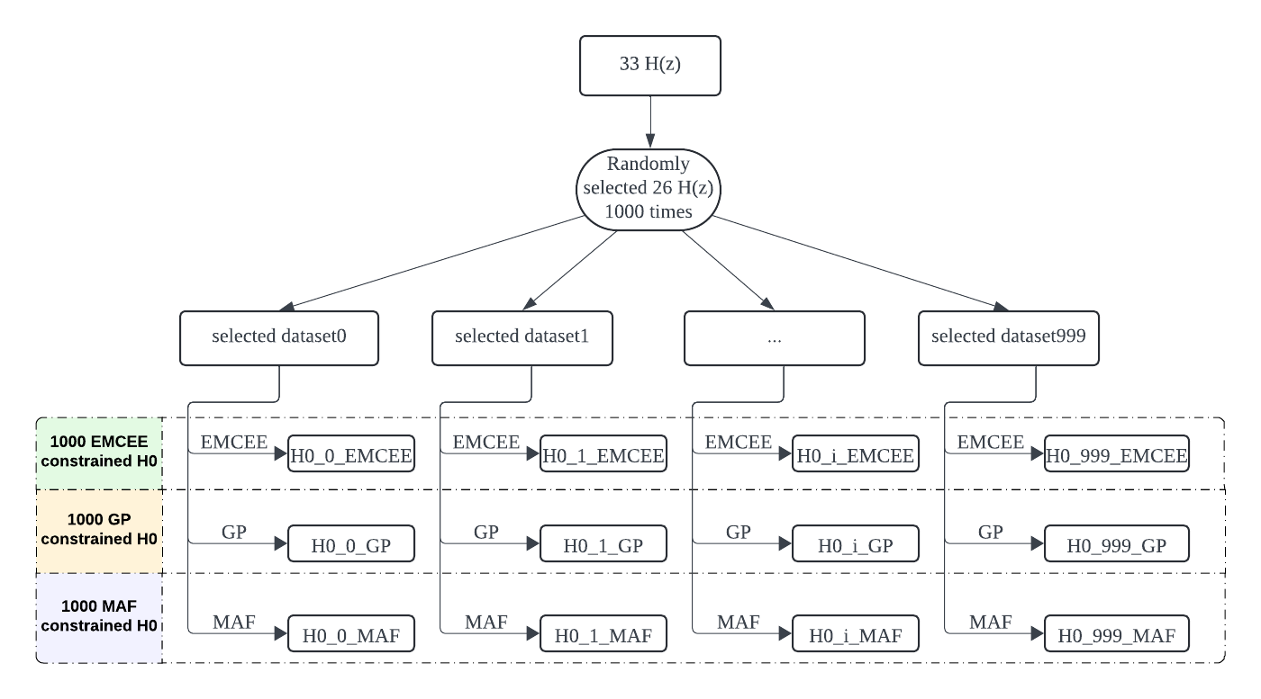
Figure 1: Diagram of MRSA procedure. At the top, 26 out of 33 $H(z)$ data points from the CC dataset are randomly selected. This is repeated 1000 times to create 1000 different datasets, shown in the middle. At the bottom, each dataset is used to constrain $\mathrm{H}_{0}$ using the EMCEE, GP, and MAF methods, resulting in 1000 $\mathrm{H}_{0}$ values for each method.

and the details are outlined as follows:

• Step 1: We randomly select a subset of data points from the CC dataset. In this paper, we randomly select 26 out of 33 $H(z)$ data points, corresponding to a $79\%$ selection rate. We then constrain $\mathrm{H}_{0}$ using these selected 26 data points, denoted as $H_{0\text{-}i\text{-}EMCEE}$, indicating the $\mathrm{H}_{0}$ constrained by EMCEE using the $i_{th}$ selected dataset.

• Step 2: We repeat Step 1 multiple times. In this paper, Step 1 is repeated $N$ times, with $N$ set to 1000. This results in the creation of 1000 randomly selected datasets, labeled with an index $i$ ranging from 0 to 999.

• Step 3: Generate 1000 constrained values of $\mathrm{H}_{0}$ with EMCEE, GP, and MAF respectively using the 1000 randomly selected $H(z)$ datasets from Step 2. Each method generates 1000 values of $\mathrm{H}_{0}$, and these results are shown in Fig. 2.

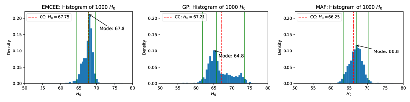
Figure 2: The histogram of 1000 constrained $\mathrm{H}_{0}$ obtained from 1000 selected $H(z)$ datasets using MRSA with EMCEE (left), GP (middle), and MAF (right). The red dashed line represents the constrained $\mathrm{H}_{0}$ using 33 CC data compiled in Table 1, while the green lines denote the $2\sigma$ range and the median of the distribution (at $2.5\%$, $50\%$, and $97.5\%$ percentile). And the mode is marked in each histogram.

To evaluate the sensitivity of $\mathrm{H}_{0}$ constraints from different methods to individual $H(z)$ data points, we propose MRSA. The distribution of 1000 constrained $\mathrm{H}_{0}$ values from selected $H(z)$ datasets is displayed in Fig. 2. we compare three metrics: (1) the absolute difference between the mode of the $\mathrm{H}_{0}$ distribution and the $\mathrm{H}_{0}$ value constrained from the full 33 CC dataset, denoted as $\Delta H_{\mathrm{0,mode-CC}}=|H_{\mathrm{0,mode}}-H_{\mathrm{0,CC}}|$, (2) the absolute difference between the median of the $\mathrm{H}_{0}$ distribution and $H_{\mathrm{0,CC}}$, denoted as $\Delta H_{\mathrm{0,median-CC}}=|H_{\mathrm{0,median}}-H_{\mathrm{0,CC}}|$, and (3) the range spanned by $2\sigma$ in the distribution, denoted as $\Delta H_{0,2\sigma}$. We summarize these results in Table 2. Here, $H_{\mathrm{0,mode}}$ represents the mode of the distribution of 1000 constrained $\mathrm{H}_{0}$ values shown in Fig. 2. The $\mathrm{H}_{0}$ value at the median density, $H_{\mathrm{0,median}}$, and the $2\sigma$ boundaries are indicated by green lines. Additionally, the red dashed line represents the Hubble constant constrained from the full 33 CC dataset, denoted as $H_{\mathrm{0,CC}}$.

We analyze the MRSA results in Fig. 2 from two perspectives to understand how different methods affect the sensitivity of constrained $\mathrm{H}_{0}$ to individual $H(z)$ data points. First, we compare the distribution of 1000 constrained $\mathrm{H}_{0}$ values from MRSA with $H_{\mathrm{0,CC}}$, which acts as the standard for $\mathrm{H}_{0}$. Each of the three methods also produces its own $H_{\mathrm{0,CC}}$ values, as shown in Fig. 2. Based on this analysis, we calculate the $\Delta H_{\mathrm{0,mode-CC}}$ and $\Delta H_{\mathrm{0,median-CC}}$ values, summarized in Table 2. The results show that, for both measures, GP values are higher than MAF, and MAF values are higher than EMCEE. This indicates that, when constraining $\mathrm{H}_{0}$, GP is more sensitive to individual $H(z)$ values than MAF, and MAF is more sensitive than EMCEE. The second perspective is the degree of dispersion in the distribution of 1000 $\mathrm{H}_{0}$ values obtained through MRSA. Greater dispersion suggests higher sensitivity to individual $H(z)$ values in constraining $\mathrm{H}_{0}$. We calculate the range of the distribution within the $2\sigma$ interval. The $\Delta H_{0,2\sigma}$ results are summarized in Table 2. These results show that GP is more sensitive to individual $H(z)$ data points than MAF, and MAF is more sensitive than EMCEE. Both perspectives confirm this finding. From this result, we infer that as more CC data are observed, the constrained $\mathrm{H}_{0}$ will vary more with GP than with MAF, and more with MAF than with EMCEE.

GP is more sensitive to individual $H(z)$ points when constraining $\mathrm{H}_{0}$ from the CC dataset compared to MAF and EMCEE. This increased sensitivity is likely due to the use of the $\Lambda$CDM model within EMCEE and MAF, as discussed in Subsec. III.1. However, this explanation is speculative, and further investigation is needed. The results in Table 2 on sensitivity to individual $H(z)$ points using three different methods help clarify how $\mathrm{H}_{0}$ constraints differ among these methods when using CC data. This information will help us choose the most suitable method for constraining $\mathrm{H}_{0}$ based on our research objectives.

Table 2: Comparing results using MRSA

Methods	$\Delta H_{\mathrm{0,mode-CC}}$	$\Delta H_{\mathrm{0,median-CC}}$	$\Delta H_{0,2\sigma}$
EMCEE	0.05	0.11	5.18
GP	2.41	1.51	11.77
MAF	0.55	0.69	6.84

III.3 Seperate to two redshift regions

In this subsection, we explore whether the constrained $\mathrm{H}_{0}$ shows different sensitivities to $H(z)$ across various redshift regions using three methods: EMCEE, GP, and MAF. We sort the 33 CC $H(z)$ datasets by redshift $z$ and divide them into two groups, with each group containing an equal number of $H(z)$ data points. Group 1 consists of 17 $H(z)$ data points from the low-redshift region, while Group 2 contains 16 $H(z)$ data points from the high-redshift region. For instance, to evaluate the sensitivity of constrained $\mathrm{H}_{0}$ to $H(z)$ in the low redshift region, we apply MRSA to this group:

• Step 1: We randomly selected 13 H(z) data points from the 17 data points in Group 1, with a selection rate of approximately $76\%$. In addition, all 16 H(z) data points from Group 2, representing the high-redshift region, are included. This results in a combined dataset of 29 $H(z)$ points: 13 from Group 1 and 16 from Group 2. To isolate the effect of the low-redshift data on $\mathrm{H}_{0}$ sensitivity, we retain all high-redshift points to prevent them from influencing the results.

• Step 2: Repeat Step 1 one thousand times to create 1000 different datasets, labeled as dataset$2_{L-i}$. In this label, ”dataset$2$” indicates that the CC data has been divided into two groups. ”$L$” refers to the selected H(z) data from the low-redshift region, while all high-redshift data is kept intact. The variable ”$i$” represents the dataset number, ranging from 0 to 999.

• Step 3: Use EMCEE, GP, and MAF to constrain $\mathrm{H}_{0}$ for the 1000 generated dataset$2_{L-i}$. The results are shown in Fig. 3.

The dataset$2_{H-i}$ is created in a similar way, by randomly selecting 13 $H(z)$ data points from the 16 data points in Group 2, and including all H(z) data points from Group 1. The results are shown in Fig. 3.

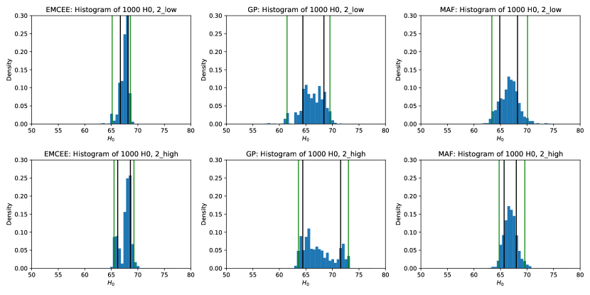
Figure 3: The histograms of the distribution of 1000 constrained $\mathrm{H}_{0}$ using the selected datasets from the CC dataset. In the first and second rows, the histograms illustrate the distribution of 1000 constrained $\mathrm{H}_{0}$ values using datasets dataset$2_{L-i}$ and dataset$2_{H-i}$, respectively. These datasets are generated in Subsec. III.3. In each row, the histograms are plotted using three different methods: EMCEE (left), GP (middle), and MAF (right). Green lines indicate the $2\sigma$ range of the distribution (at $2.5\%$ and $97.5\%$ percentiles), while black lines represent the $1\sigma$ range (at $16\%$ and $84\%$ percentiles).

By analyzing Fig. 3, we can assess whether H(z) values from different redshift regions have varying impacts on the sensitivity of the constrained $\mathrm{H}_{0}$. The wider range of $\mathrm{H}_{0}$ within the $1\sigma$ ($\Delta H_{0,1\sigma}$) and $2\sigma$ ($\Delta H_{0,2\sigma}$) intervals indicates greater sensitivity of constrained $\mathrm{H}_{0}$ to individual $H(z)$ data points in the corresponding redshift region for that method. To compare the sensitivity of constrained $\mathrm{H}_{0}$ to individual $H(z)$ data points across different redshift regions, we divide the redshift into two regions and calculate

$$\Delta H_{0,1\sigma,\mathrm{L-H}}=\Delta H_{0,1\sigma,\mathrm{Low}}-\Delta H_{0,1\sigma,\mathrm{High}},$$ (20)

$$\Delta H_{0,2\sigma,\mathrm{L-H}}=\Delta H_{0,2\sigma,\mathrm{Low}}-\Delta H_{0,2\sigma,\mathrm{High}}.$$ (21)

where $\Delta H_{0,1\sigma,\mathrm{Low}}$ refers to the $\mathrm{H}_{0}$ range within the $1\sigma$ area in the first row of Fig. 3, while $\Delta H_{0,1\sigma,\mathrm{High}}$ refers to the $1\sigma$ area in the second row. The same applies for $\Delta H_{0,2\sigma,\mathrm{Low}}$ and $\Delta H_{0,2\sigma,\mathrm{High}}$. The results of $\Delta H_{0,1\sigma,\mathrm{L-H}}$ and $\Delta H_{0,2\sigma,\mathrm{L-H}}$ for three different methods in Fig. 3 are summarized in Table 3.

Table 3: The comparison of 2 separate regions

Methods	$\Delta H_{0,1\sigma,\mathrm{L-H}}$	$\Delta H_{0,2\sigma,\mathrm{L-H}}$
EMCEE	-0.95	-0.30
GP	-3.16	-1.33
MAF	1.05	1.90

In Equation (20), if $\Delta H_{0,1\sigma,\mathrm{L-H}}>0$, it means that $\Delta H_{0,1\sigma,\mathrm{Low}}$ is greater than $\Delta H_{0,1\sigma,\mathrm{High}}$, indicating that the constrained $\mathrm{H}_{0}$ is more responsive to the $H(z)$ in the low redshift region than in the high redshift region. On the other hand, if $\Delta H_{0,1\sigma,\mathrm{L-H}}<0$, it shows that the constrained $\mathrm{H}_{0}$ is less sensitive to the $H(z)$ in the low redshift region than in the high redshift region. Table 3 shows that for the EMCEE and GP methods, the constrained $\mathrm{H}_{0}$ s more sensitive to $H(z)$ data in the high redshift region than in the low redshift region, as indicated by $\Delta H_{0,1\sigma,\mathrm{L-H}}$ and $\Delta H_{0,2\sigma,\mathrm{L-H}}$ being less than 0. In contrast, the MAF method shows that the constrained $\mathrm{H}_{0}$ is more sensitive to $H(z)$ data in the low redshift region than in the high redshift region.

All three methods (EMCEE, GP, and MAF) are sensitive to individual data points in both low and high redshift regions. For MAF, the constrained $\mathrm{H}_{0}$ shows higher sensitivity to individual $H(z)$ data points in the lower redshift region. This is expected, as $H(z)$ becomes increasingly influential on the constrained H0 as it approaches $z=0$. In contrast, for EMCEE and GP, the constrained $\mathrm{H}_{0}$ is more sensitive to $H(z)$ data in higher redshift regions. This difference may be due to the inherent characteristics of the EMCEE and GP methods or the limited amount of $H(z)$ data in the CC dataset, which makes the conclusions less generalizable. To understand these factors better, we will investigate why EMCEE and GP lead to greater sensitivity to $H(z)$ in the high redshift region. In future research, we will explore the impact of EMCEE and GP in greater detail and utilize a larger dataset of observed CC data to achieve more accurate results.

IV Simulation

The $\mathrm{H}_{0}$ constraint differs when using the CC dataset with three different methods: EMCEE, GP, and MAF. In Subsec. III.2, we compare their sensitivity in constraining $\mathrm{H}_{0}$ to individual $H(z)$ values using MRSA. In this section, we focus on comparing the accuracy of $\mathrm{H}_{0}$ constraints obtained by these three methods. First, we simulate a set of $H(z)$ values with a prior $\mathrm{H}_{0}$ ($\mathrm{H}_{\mathrm{0prior}}$) based on the observed CC data. Next, we apply each of the three methods to the simulated $H(z)$ dataset to constrain $\mathrm{H_{0sim}}$. The accuracy of each method is evaluated by comparing $\mathrm{H_{0sim}}$ to the prior $\mathrm{H}_{\mathrm{0prior}}$, with greater accuracy indicated by $\mathrm{H_{0sim}}$ being closer to the prior $\mathrm{H}_{\mathrm{0prior}}$. To reduce the effect of random variations in each simulation, we generate 100 simulated datasets and compare the mean and mean square error of 100 $\mathrm{H_{0sim}}$ values to the prior $\mathrm{H}_{\mathrm{0prior}}$. Additionally, to minimize the influence of the simulation approach, we employ two simulation methods: one based on the $\Lambda$CDM model and the other on the Gaussian Process.

IV.1 Simulation based on $\Lambda$CDM

To simulate $H(z)$ values based on the observed CC data with the prior $\mathrm{H}_{\mathrm{0prior}}$, we adopt and improve upon the simulation method from Ma and Zhang [23]. The simulated Hubble parameter, $H_{\mathrm{sim}}$, at redshift $z_{\mathrm{sim}}$ is

$$H_{\mathrm{sim}}(z_{\mathrm{sim}})=H_{\mathrm{fid}}(z_{\mathrm{sim}})+\sigma_{\mathrm{sim}}(z_{\mathrm{sim}}).$$ (22)

Here, $z_{\mathrm{sim}}$ denotes the redshift corresponding to $H_{\mathrm{sim}}$. $H_{\mathrm{fid}}(z_{\mathrm{sim}})$ indicates the value calculated from the fiducial model, while $\sigma_{\mathrm{sim}}(z_{\mathrm{sim}})$ represents the simulated uncertainty at each redshift $z_{\mathrm{sim}}$. In Equation (22), in order to generate the $H_{\mathrm{sim}}(z_{\mathrm{sim}})$ dataset, we need to determine the values of redshift $z_{\mathrm{sim}}$, $H_{\mathrm{fid}}(z_{\mathrm{sim}})$ and $\sigma_{\mathrm{sim}}(z_{\mathrm{sim}})$ at each redshift.

First, to ensure the simulated dataset closely matches the observed CC dataset, we generate 33 values for $z_{\mathrm{sim}}$ within the range [0, 2.5]. We maintain the same distribution density of $z_{\mathrm{sim}}$ values as in the CC dataset. Next, we compute $H_{\mathrm{fid}}(z_{\mathrm{sim}})$ based on the $\Lambda$CDM model,

$$H_{\mathrm{fid}}(z_{\mathrm{sim}})=\mathrm{H}_{0}\sqrt{\Omega_{M}(1+z_{\mathrm{sim}})^{3}+(1-\Omega_{M})}.$$ (23)

In Equation (23), to calculate $H_{\mathrm{fid}}(z_{\mathrm{sim}})$, we need the values of $\mathrm{H}_{0}$ and $\Omega_{M}$. Here, we apply the $\mathrm{H}_{0}$ prior and $\Omega_{M}$ prior, denoted as $\mathrm{H}_{\mathrm{0prior}}$ and $\Omega_{M\text{prior}}$, to estimate $\mathrm{H}_{0}$ and $\Omega_{M}$ in Equation (23). To determine appropriate values for $\mathrm{H}_{\mathrm{0prior}}$ and $\Omega_{M\text{prior}}$, we constrain them using the observed CC data through EMCEE, obtaining $\mathrm{H}_{\mathrm{0prior}}=67.75\pm 3.08\,\mathrm{km\,s^{-1}\,Mpc^{-1}}$ and $\Omega_{M\text{prior}}=0.328\pm 0.061$. For each data point at redshift $z_{\mathrm{sim}}$, we draw random values of $\mathrm{H}_{0}$ and $\Omega_{M}$ from Gaussian distributions: $\mathrm{H}_{0}\thicksim\mathcal{N}(67.75,3.08)\,\mathrm{km\,s^{-1}\,Mpc^{-1}}$ and $\Omega_{M}\thicksim\mathcal{N}(0.328,0.061)$. Since each simulated dataset contains 33 $H_{\mathrm{fid}}(z_{\mathrm{sim}})$ values, we sample random $\mathrm{H}_{0}$ and $\Omega_{M}$ values 33 times. Using these sampled $\mathrm{H}_{0}$ and $\Omega_{M}$ values along with the corresponding redshift $z_{\mathrm{sim}}$, we compute all 33 values of $H_{\mathrm{fid}}(z_{\mathrm{sim}})$ using Equation (23).

Finally, we generate $\sigma_{\mathrm{sim}}(z_{\mathrm{sim}})$ at each redshift $z_{\mathrm{sim}}$ using the method proposed by Ma and Zhang [23]. The simulated $\sigma_{\mathrm{sim}}$ is based on the $\sigma_{H}$ of the observed CC data, as shown in Fig. 4.

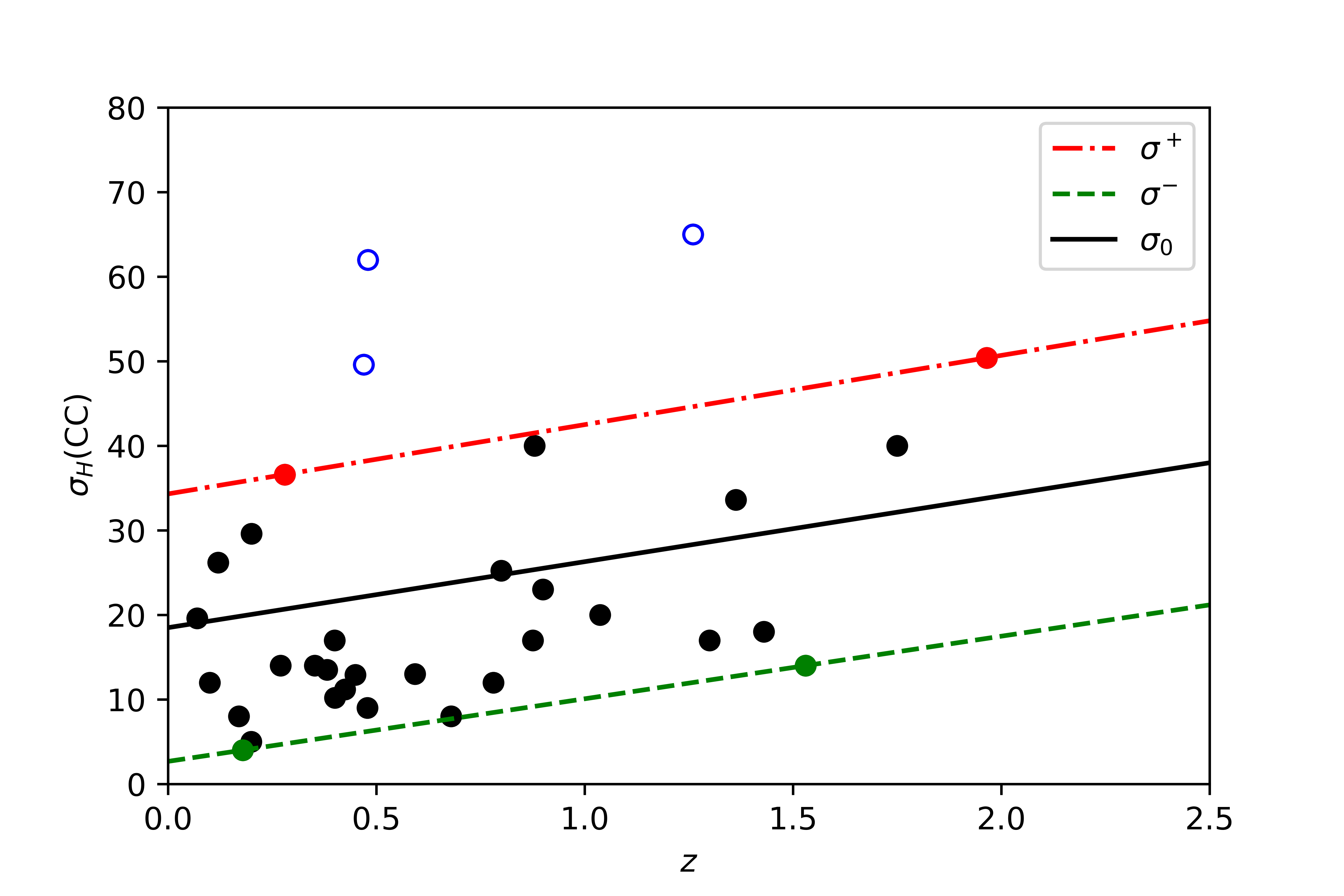
Figure 4: The 1$\sigma$ uncertainty of CC data. Black dots represent non-outliers, while blue circles indicate outliers. The red dash-dotted line and the green dashed line mark the bounds of the non-outliers, denoted as $\sigma^{+}$ and $\sigma^{-}$, respectively. The solid black line represents the mean uncertainty of the non-outliers, denoted as $\sigma_{0}$.

In the figure, the trend of $\sigma_{H}$ is bounded by two straight lines, excluding the outliers. We assume that this bounded region contains 95$\%$ of the $\sigma_{H}$ values and that $\sigma_{H}$ follows a Gaussian distribution. Thus, we simulate $\sigma_{\mathrm{sim}}$ in Equation (22) as $\mathcal{N}(\sigma_{0},\frac{\sigma^{+}+\sigma^{-}}{4})$ at each redshift $z_{\mathrm{sim}}$, as illustrated in Fig. 5.

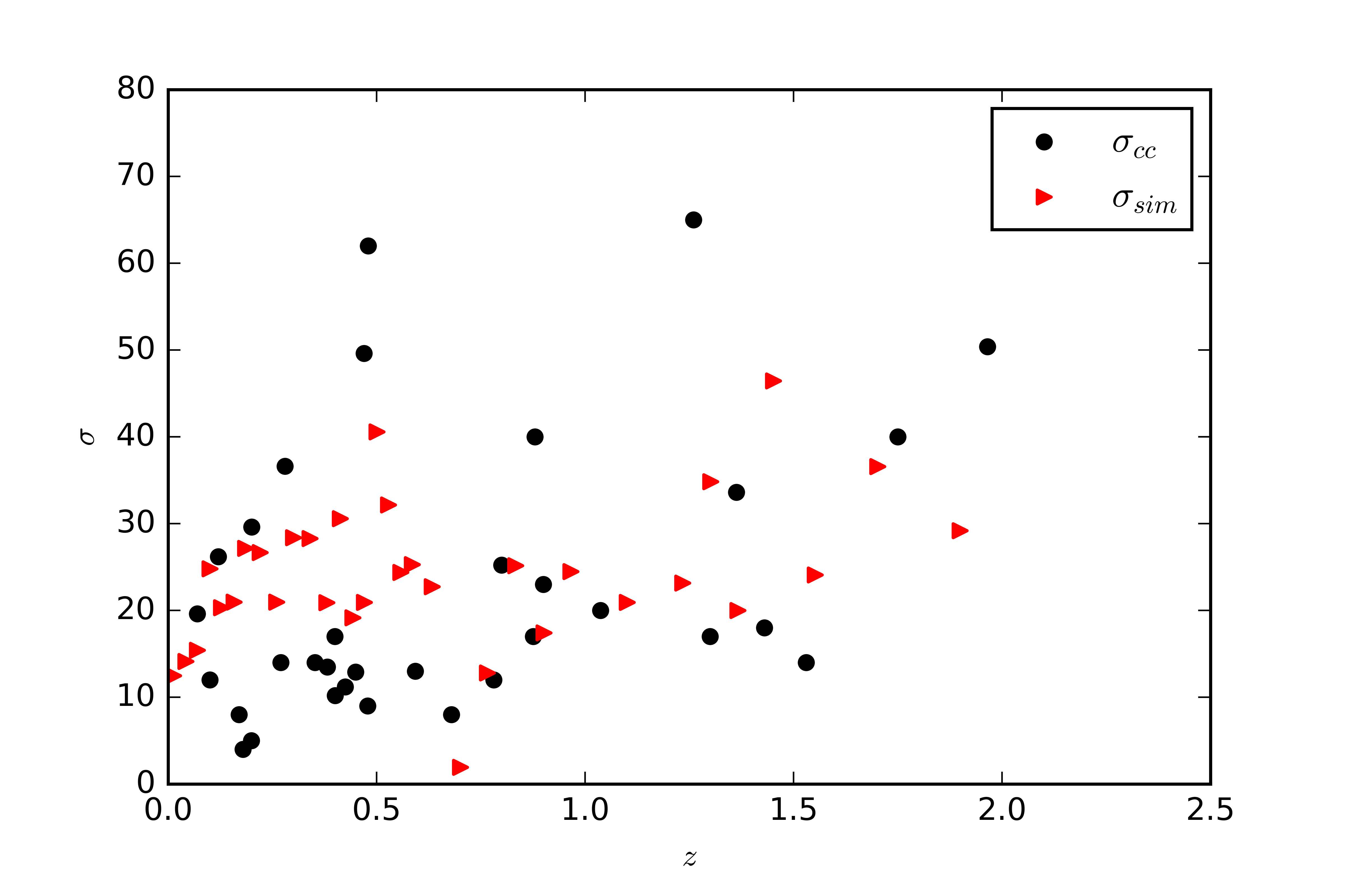
Figure 5: The simulated $\sigma_{\mathrm{sim}}$. The black dots represent the observed uncertainty $\sigma_{cc}$ from CC data, while red triangles represent the simulated uncertainty $\sigma_{\mathrm{sim}}$.

At this stage, we have generated $z_{\mathrm{sim}}$, $H_{\mathrm{fid}}(z_{\mathrm{sim}})$ and $\sigma_{\mathrm{sim}}(z_{\mathrm{sim}})$ in Equation (22). By combining these components, we can generate a simulated dataset consisting of 33 $H_{\mathrm{sim}}(z_{\mathrm{sim}})$ data points based on the $\Lambda$CDM, as depicted in Fig. 6.

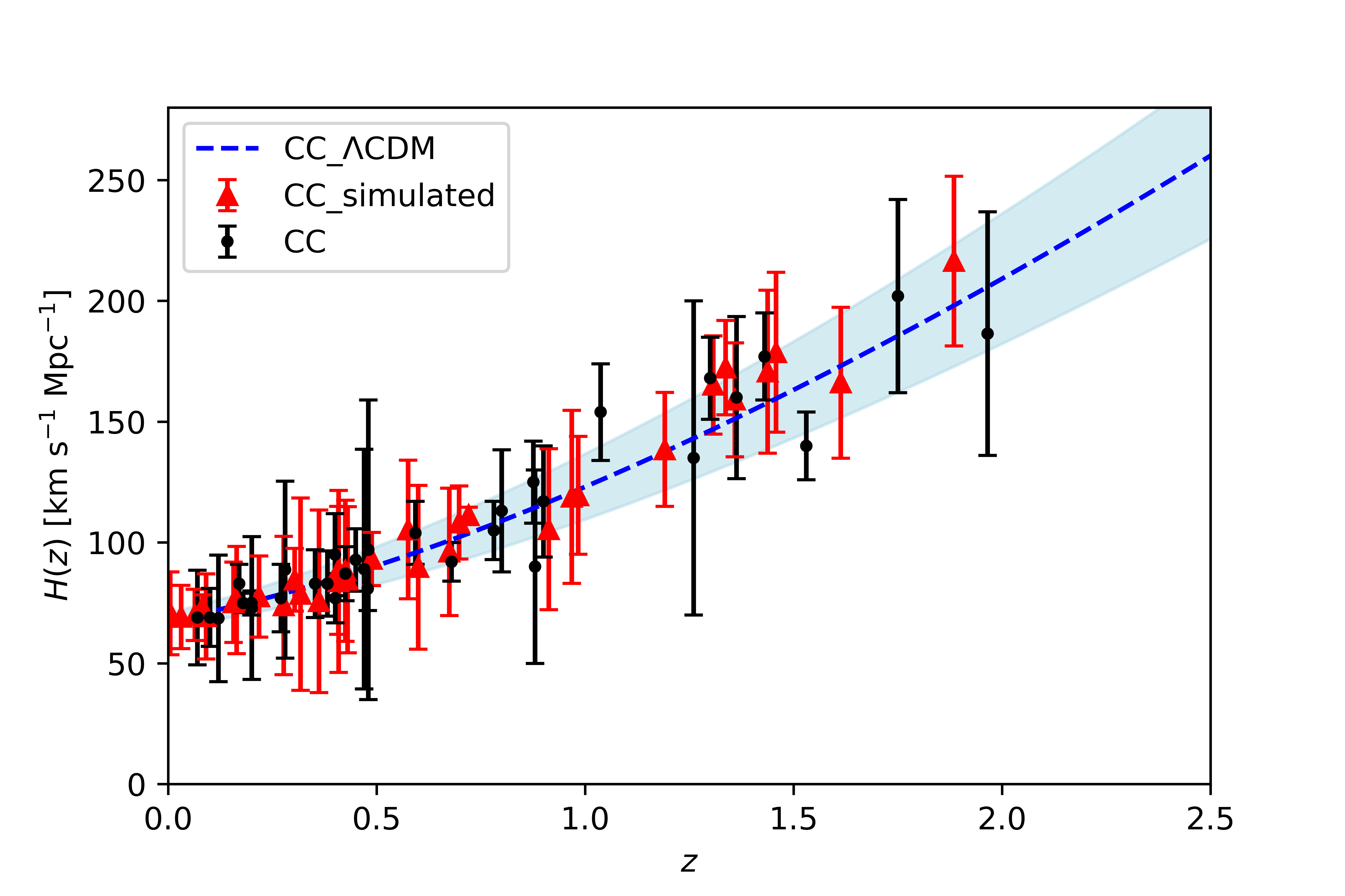
Figure 6: The simulated $H(z)$ dataset based on the $\Lambda$CDM model using CC data. The simulated data points, $H_{\text{sim}}(z_{\text{sim}})$, are shown as red triangles with error bars. For comparison, the observational CC data are represented by black dots with error bars. The $\Lambda$CDM model used to generate the fiducial values, $H_{\text{fid}}(z_{\text{sim}})$, is depicted by the blue dashed line, with the shaded area indicating the $1\sigma$ confidence interval.

We then constrain $\mathrm{H_{0sim}}$ using the simulated dataset with EMCEE, GP, and MAF.

To minimize the impact of randomness in generating the $H_{\mathrm{sim}}(z_{\mathrm{sim}})$ dataset, we create 100 simulated $H_{\mathrm{sim}}(z_{\mathrm{sim}})$ datasets. This approach allows us to obtain 100 $\mathrm{H_{0sim}}$ values using EMCEE, GP, and MAF as illustrated in Fig. 7.

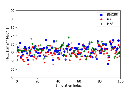
Figure 7: The constrained 100 $\mathrm{H_{0sim}}$ values obtained with EMCEE (blue dots), GP (red stars), and MAF (green pluses) using 100 $H(z)$ datasets simulated based on $\Lambda$CDM model. The black line represents the prior of $\mathrm{H}_{0}$, with $\mathrm{H}_{\mathrm{0prior}}=67.75\pm 3.08\,\mathrm{km\,s^{-1}\,Mpc^{-1}}$.

We calculate the mean and standard deviation of 100 $\mathrm{H_{0sim}}$ for each method, as presented in Table 4.

Table 4: The mean and standard deviation of 100 $\mathrm{H_{0sim}}$

Methods	mean	standard deviation
EMCEE	66.63	2.76
GP	64.80	2.87
MAF	66.46	2.82
$\mathrm{H}_{\mathrm{0prior}}=67.75\pm 3.08$

To determine which method (EMCEE, GP, and MAF) most accurately constrains $\mathrm{H}_{0}$ to the prior value $\mathrm{H}_{\mathrm{0prior}}$, we compare the mean of 100 constrained $\mathrm{H_{0sim}}$ values with $\mathrm{H}_{\mathrm{0prior}}$. Table 4 shows that the mean of 100 $\mathrm{H_{0sim}}$ values from EMCEE is closer to $\mathrm{H}_{\mathrm{0prior}}$ than the mean values from GP and MAF. Furthermore, the mean value from MAF is closer to $\mathrm{H}_{\mathrm{0prior}}$ than the mean value from GP. These findings indicate that EMCEE is more accurate in constraining $\mathrm{H}_{0}$ compared to MAF, and MAF is more accurate than GP when simulating the $H_{\mathrm{sim}}(z_{\mathrm{sim}})$ dataset based on $\Lambda$CDM.

IV.2 Simulation based on Gaussian Process

In Subsec. IV.1, we compare the accuracy of three different methods in constraining $\mathrm{H}_{0}$ using $H(z)$ datasets simulated based on $\Lambda$CDM model. To examine the influence of different simulated model on this study, we simulated $H(z)$ dataset in this subsection based on the Gaussian Process.

We aim to simulate a dataset as follows:

$$H_{\mathrm{sim}}(z_{\mathrm{sim}})=H_{\mathrm{GP}}(z_{\mathrm{sim}})+\sigma_{\mathrm{sim}}(z_{\mathrm{sim}}).$$ (24)

This dataset contains 33 data points based on the Gaussian Process, according to the CC dataset presented in Table 1. The redshift $z_{\mathrm{sim}}$ is generated with the same distribution density as in the CC dataset. First, we need to select an appropriate prior, $\mathrm{H}_{\mathrm{0prior}}$, for this simulation. Since this simulation is based on the Gaussian Process, we reconstruct the 33 CC data points in Table 1 and select the reconstructed $\mathrm{H}_{0}$ as the prior: $\mathrm{H}_{\mathrm{0prior}}=67.21\pm 4.72\,\mathrm{km\,s^{-1}\,Mpc^{-1}}$. Next, we add this $\mathrm{H}_{\mathrm{0prior}}$ at redshift $z=0$ to the 33 observed CC data points. Using the Gaussian Process, we then reconstruct these 34 $H(z)$ data points. The distributions of $H_{\mathrm{GP}}(z_{\mathrm{sim}})$ are displayed in Fig. 8.

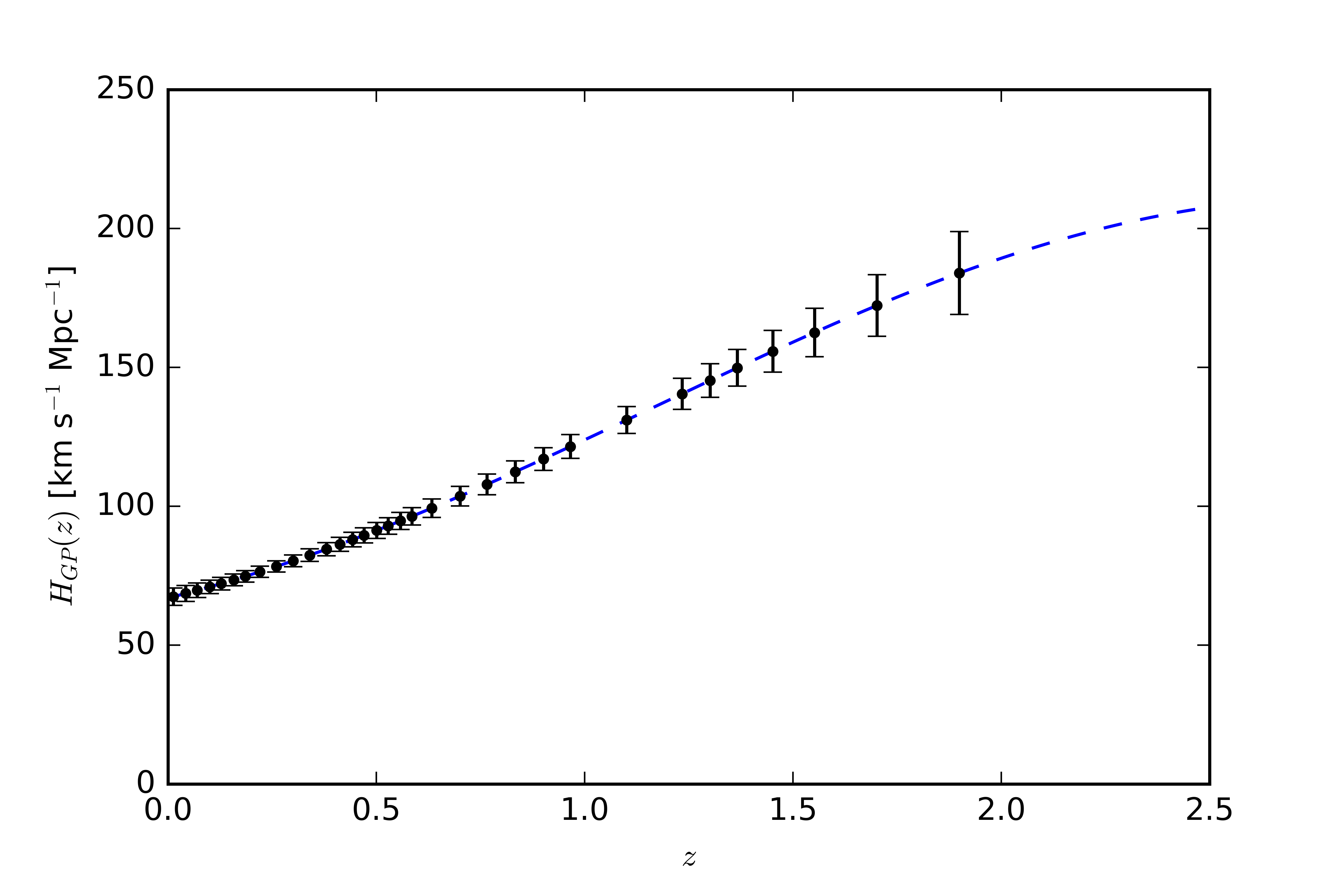
Figure 8: Distribution of $H_{\mathrm{GP}}$ in Equation (24). The black dots with error bars represent the mean and $1\sigma$ values of $H_{\mathrm{GP}}(z_{\mathrm{sim}})$ at different redshifts $z_{\mathrm{sim}}$. The blue dashed line shows the distribution of the mean of $H_{\mathrm{GP}}$ as described in Equation (24).

We assume that $H_{\mathrm{GP}}(z_{\mathrm{sim}})$ follows a Gaussian distribution, with the mean and variance at each redshift $z_{\mathrm{sim}}$ shown in Fig. 8. Thus, we randomly generate 33 values of $H_{\mathrm{GP}}(z_{\mathrm{sim}})\thicksim\mathcal{N}(H_{\mathrm{GP\_mean}}(z_{\mathrm{sim}}),\sigma(z_{\mathrm{sim}}))$ at redshift $z_{\mathrm{sim}}$, as defined in Equation (24). Next, we simulate $\sigma_{\mathrm{sim}}(z_{\mathrm{sim}})$ in Equation (24) using the same method described in Subsec. IV.1. At this stage, we have simulated 33 values of $H_{\mathrm{sim}}(z_{\mathrm{sim}})$, as illustrated in Fig. 9.

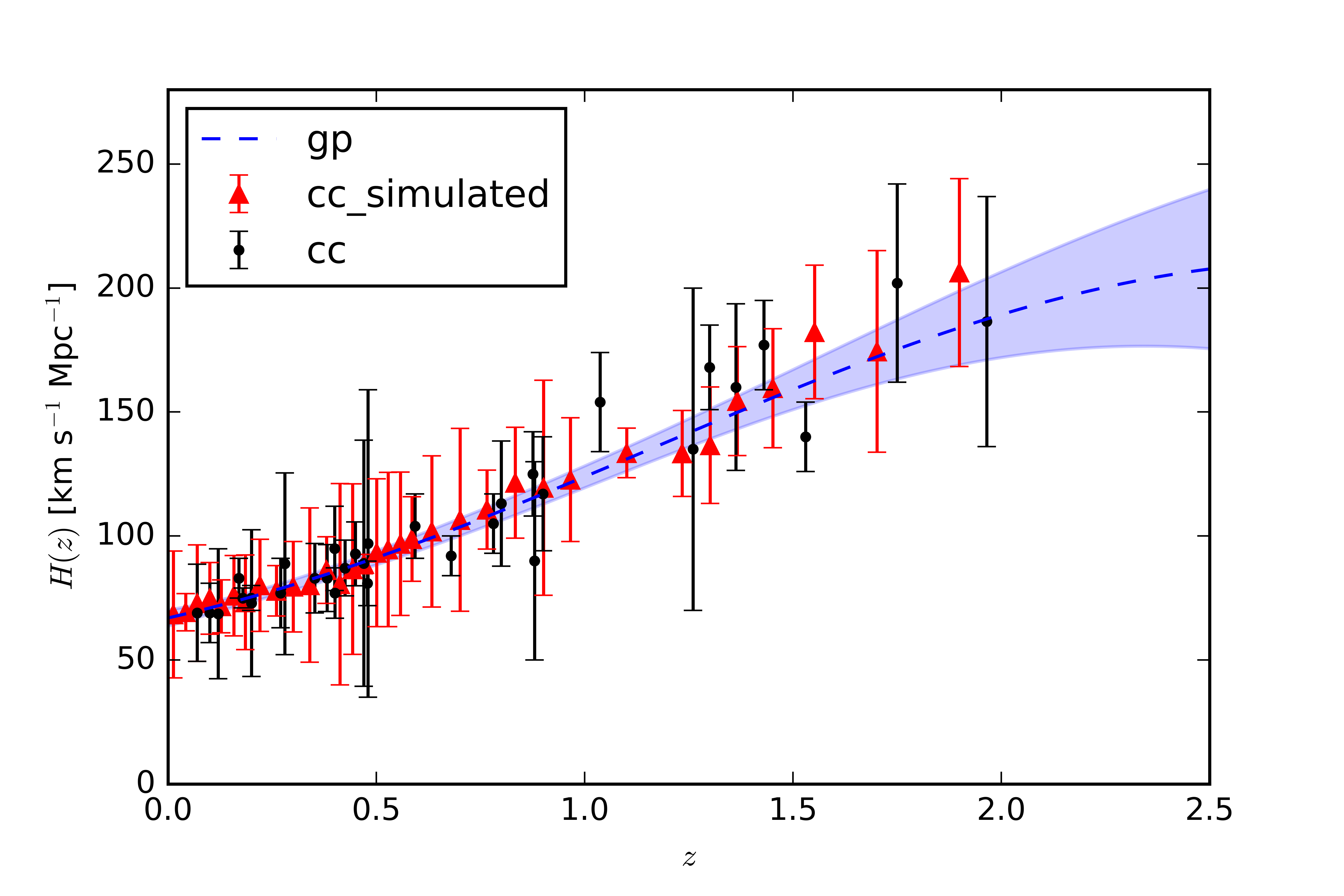
Figure 9: The simulated $H(z)$ dataset based on the Gaussian Process using CC data. The simulated data points, $H_{\text{sim}}(z_{\text{sim}})$, are shown as red triangles with error bars. For comparison, the observational CC data are represented by black dots with error bars. The Gaussian Process used to generate the values of $H_{\text{GP}}(z_{\text{sim}})$ in Equation (24), is depicted by the blue dashed line, with the shaded area indicating the $1\sigma$ confidence interval.

We then constrain $\mathrm{H_{0sim}}$ using the simulated dataset with EMCEE, GP, and MAF.

As in Subsec. IV.1, we simulate 100 datasets, each containing 33 $H_{\mathrm{sim}}(z_{\mathrm{sim}})$ data points, to reduce the impact of randomness in individual simulations. As a result, we obtain 100 $\mathrm{H_{0sim}}$ values using EMCEE, GP, and MAF, respectively, as shown in Fig. 10.

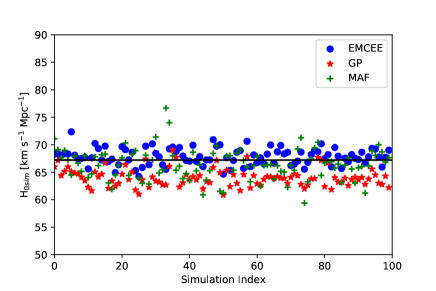
Figure 10: The constrained 100 $\mathrm{H_{0sim}}$ values obtained with EMCEE (blue dots), GP (red stars), and MAF (green pluses) using 100 $H(z)$ datasets simulated based on Gaussian Process. The black line represents the prior of $\mathrm{H}_{0}$, with $\mathrm{H}_{\mathrm{0prior}}=67.21\pm 4.72\,\mathrm{km\,s^{-1}\,Mpc^{-1}}$.

To compare the accuracy of different methods in constraining $\mathrm{H_{0sim}}$ using 100 simulated $H_{\mathrm{sim}}(z_{\mathrm{sim}})$ datasets, we calculate the mean and standard deviation of the 100 $\mathrm{H_{0sim}}$ values for each method, as shown in Fig. 10 and presented in Table 5.

Table 5: The mean and standard deviation of 100 $\mathrm{H_{0sim}}$

Methods	mean	standard deviation
EMCEE	67.85	1.51
GP	64.02	1.61
MAF	66.39	2.77
$\mathrm{H}_{\mathrm{0prior}}=67.21\pm 4.72$

Table 5 shows that the mean of the 100 $\mathrm{H_{0sim}}$ values from EMCEE is closer to $\mathrm{H}_{\mathrm{0prior}}$ than the means from GP and MAF. Additionally, the mean from MAF is closer to $\mathrm{H}_{\mathrm{0prior}}$ than that from GP. These findings indicate that EMCEE is more accurate in constraining $\mathrm{H}_{0}$ than MAF, and MAF is more accurate than GP when simulating the $H(z)$ dataset based on the Gaussian Process. This result is consistent with the findings in Subsec. IV.1, indicating that the accuracy of different methods in constraining $\mathrm{H}_{0}$ is independent of the simulation method, whether the $H_{\mathrm{sim}}(z_{\mathrm{sim}})$ datasets are generated based on the $\Lambda$CDM model or the Gaussian Process.

V discussions and conclusions

The Hubble constant ($\mathrm{H}_{0}$) is crucial for understanding the evolution of the universe. However, a significant 5$\sigma$ discrepancy exists between the two main methods for measuring $\mathrm{H}_{0}$ [1, 2], known as the Hubble tension. Another approach to determining $\mathrm{H}_{0}$ is using Cosmic Chronometers, a model-independent method for measuring $H(z)$. The CC dataset is presented in Table 1. This method may provide valuable insights into resolving the Hubble tension. Various methods can be used to constrain $H(z)$, including EMCEE, GP, and MAF, as introduced in Subsec. III.1. EMCEE is an affine-invariant ensemble sampler for MCMC, GP is a non-parametric method that provides a model-independent reconstruction of the Hubble parameter, and MAF is a deep learning-based approach capable of modeling complex distributions.

The $\mathrm{H}_{0}$ results derived from these three methods using the same CC data differ noticeably. This discrepancy highlights the importance of understanding the strengths and limitations of each method in the context of cosmological data. Despite the potential of each technique, a comprehensive study comparing these methods for constraining $\mathrm{H}_{0}$ from $H(z)$ is lacking. This study seeks to address this gap by comparing EMCEE, GP, and MAF methods for constraining $\mathrm{H}_{0}$ using $H(z)$ data. By evaluating their performance, we aim to identify the most suitable method for different research contexts, ultimately leading to more accurate and reliable determinations of the Hubble constant and a deeper understanding of the universe’s expansion history. We compare these three methods by evaluating their sensitivity to individual $H(z)$ data points and their accuracy in constraining $\mathrm{H}_{0}$ using simulated $H(z)$ datasets.

In Subsec. III.2, we propose MRSA to test the sensitivity of the three methods to individual $H(z)$ data points. The MRSA method randomly selects 26 out of 33 $H(z)$ data points from the CC dataset to create a new dataset. To reduce the impact of random selection, we generate 1000 different datasets. We then constrain 1000 $\mathrm{H}_{0}$ values using these datasets with EMCEE, GP, and MAF, respectively. The distributions are shown in Fig. 2, while the comparison results are summarized in Table 2. Our findings indicate that the GP method is more sensitive to individual $H(z)$ points than both MAF and EMCEE, likely because the $\Lambda$CDM model is applied in EMCEE and MAF. Additionally, MAF demonstrates greater sensitivity than EMCEE. This suggests that as more data points are obtained, the $\mathrm{H}_{0}$ value constrained by GP will show greater variation compared to those from EMCEE and MAF. To investigate whether this sensitivity relates to the redshift range of the $H(z)$ data points, we split the CC dataset into two groups and applied the MRSA to each group in Subsec. III.3. Our analysis reveals that all three methods (EMCEE, GP, and MAF) are sensitive to individual data points in both low and high redshift regions. Specifically, for EMCEE and GP, $\mathrm{H}_{0}$ is more sensitive to higher redshift $H(z)$ data points, while for MAF, $\mathrm{H}_{0}$ is more sensitive to lower redshift $H(z)$ data points. This difference may result from the inherent differences in the methods themselves, or it could simply be caused by the small number of data points in the CC dataset. Future research will further investigate this sensitivity across different redshift regions using a larger CC dataset, aiming to obtain more accurate results.

In Sec. IV, we test the accuracy of EMCEE, GP, and MAF in constraining $\mathrm{H}_{0}$ using CC data by simulating the $H_{\mathrm{sim}}(z_{\mathrm{sim}})$ dataset with a prior $\mathrm{H}_{\mathrm{0prior}}$. We then use each method to constrain $\mathrm{H_{0sim}}$ from the simulated dataset. The method that produces an $\mathrm{H}_{0}$ closest to the prior $\mathrm{H}_{\mathrm{0prior}}$ is considered the most accurate. To reduce the influence of different simulation methods, we use two approaches: Simulation based on $\Lambda$CDM (Subsec. IV.1) and Simulation based on Gaussian Process (Subsec. IV.2). To reduce the impact of randomness in the simulated datasets, we generate 100 different $H_{\mathrm{sim}}(z_{\mathrm{sim}})$ datasets. For each simulated dataset, we apply all three methods to constrain $\mathrm{H_{0sim}}$. We then compare the mean values of the 100 constrained $\mathrm{H_{0sim}}$ results from each method to the prior $\mathrm{H}_{\mathrm{0prior}}$. The comparison results are presented in Table 4 and Table 5. Our findings indicate that EMCEE is more accurate than MAF, and MAF is more accurate than GP, regardless of the simulation method.

By comparing the sensitivity and accuracy of EMCEE, GP, and MAF, we gain a deeper understanding into their respective features. This knowledge helps identify the most suitable method for a range of research applications, extending beyond cosmology to fields like medicine [30, 31] and economics [32, 33]. However, this study has several limitations: (1) The accuracy comparison relies on two simulation approaches introduced in Subsec. IV.1 and IV.2, which may not be universally applicable. (2) The accuracy results are derived from simulations using a prior $\mathrm{H}_{0}$, rather than actual observational data. (3) While we compared sensitivity and accuracy, we did not assess the overall characteristics of the methods. (4) The limited amount of $H(z)$ data in the CC dataset may have affected our results.

Future research will focus on generating simulated $H_{\mathrm{sim}}(z_{\mathrm{sim}})$ datasets using a wider variety of improved simulation methods. This approach will help minimize the impact of specific simulation methods on accuracy comparisons. Additionally, we will explore the characteristics of EMCEE, GP, and MAF in greater depth to gain a more comprehensive understanding of each method. By incorporating more $H(z)$ data points into our analysis, we aim to achieve more reliable comparisons of the sensitivity and accuracy of these methods. This will result in more precise determinations of $\mathrm{H}_{0}$ and offer deeper insights into the universe’s expansion.