Approximation of Permutation Invariant Polynomials by Transformers: Efficient Construction in Column-Size
Abstract.
Transformers are a type of neural network that have demonstrated remarkable performance across various domains, particularly in natural language processing tasks. Motivated by this success, research on the theoretical understanding of transformers has garnered significant attention. A notable example is the mathematical analysis of their approximation power, which validates the empirical expressive capability of transformers. In this study, we investigate the ability of transformers to approximate column-symmetric polynomials—an extension of symmetric polynomials that take matrices as input. Consequently, we establish an explicit relationship between the size of the transformer network and its approximation capability, leveraging the parameter efficiency of transformers and their compatibility with symmetry by focusing on the algebraic properties of symmetric polynomials.
1. Introduction
The Transformer, a neural network extension proposed by Vaswani et al. (2017), has played a central role in data-driven large language models such as the Generative Pre-trained Transformer (GPT) (Brown et al. (2020)) and Bidirectional Encoder Representations from Transformers (BERT) (Devlin et al. (2018)), becoming a primary focus in natural language processing tasks. It is also well known for its high performance in tasks beyond natural language processing, such as image processing (Dosovitskiy et al. (2021)), where convolutional neural networks have traditionally dominated, thereby broadening its range of applications.
The property that neural networks and Transformers can represent a wide range of functions is called the universal approximation property and has been extensively studied. While it is widely known that neural networks can approximate any continuous function to an arbitrary degree of accuracy (e.g., Cybenko (1989); Hornik (1991); Yarotsky (2017); Lu et al. (2021)), it has also been shown that Transformers exhibit similar properties. For a representative example, Yun et al. (2019) demonstrated that Transformers possess the universal approximation property, allowing them to approximate permutation equivariant functions (i.e., when the columns of the input matrix are swapped, the entries of the output matrix change in the same way) with matrix inputs.
An important challenge in Transformer theory is the rigorous investigation of its approximation efficiency. For example, in Yun et al. (2019), the number of parameters required to construct the approximating Transformer increases exponentially with the size of the input matrix, highlighting significant room for improvement in approximation efficiency. Kajitsuka and Sato (2024) reveals that a Transformer with a single attention layer is a universal approximator of permutation equivariant functions. Takakura and Suzuki (2023) investigates a special class of functions on an infinite-dimensional set and shows that Transformers can approximate such functions with a number of parameters that does not depend on the infinite dimensionality. Despite these results, the efficiency of Transformers in approximating a general class of functions remains an ongoing area of research.
In this paper, we focus on approximating permutation invariant polynomials and study the approximation efficiency of Transformers. Since Transformers are permutation equivariant, it is natural to consider permutation invariant functions when approximating functions with a one-dimensional output. In addition, since analytic functions can be arbitrarily well approximated by polynomials, it makes sense to restrict the target function to polynomials, which are relatively easy to approximate. We demonstrate explicit relationships between the width and depth of the Transformer network and its approximation error. We also focus on parameter efficiency: in our approximation, the number of parameters is independent of the number of columns in the input matrices. This result contrasts with conventional neural networks, where the number of parameters increases as the input dimension increases. The proof is constructive, providing explicit parameter configurations for the approximating Transformer.
To prove the result above, we extend symmetric polynomials to matrices and focus on approximating column-symmetric polynomials. While it is known that any symmetric polynomial can be expressed as a linear combination of monomial symmetric polynomials, we utilize the analogous result that any column-symmetric polynomial can be expressed as a linear combination of monomial column-symmetric polynomials. In constructing monomial column-symmetric polynomials, we focus on their algebraic properties, particularly the number of columns involved in the polynomial terms (referred to as the rank in this paper). By discussing these polynomials inductively based on their rank, we derive the network size required to approximate monomial column-symmetric polynomials and analyze the approximation errors.
1.1. Related Works
As this research concerns universal approximation, we discuss several related works on this topic.
1.1.1. Approximation Theory of Neural Networks
The universal approximation theorem was established by works such as Cybenko (1989) and Hornik (1991). These demonstrate that single-layer neural networks with a general activation function can approximate any continuous function on compact domains to an arbitrary degree of precision. However, they focus solely on the existence of neural networks that approximate continuous functions and do not specify their exact architecture.
In recent years, the empirical success of deep neural networks in tasks such as image recognition and object detection has sparked significant interest in their representational abilities. Yarotsky (2017) showed that deep neural networks can approximate smooth functions with fewer parameters than shallow ones. Further developments include the results of Lu et al. (2017), which showed that ReLU FNNs with a fixed width and arbitrary depth can approximate any Lebesgue-integrable function to an arbitrary degree of precision in the sense of . Lu et al. (2021) proved that -functions can be uniformly approximated with an error that decreases at a polynomial rate with respect to the number of layers and width. In addition, Lu et al. (2021) showed that the polynomial order of the uniform approximation error is optimal, except for a logarithmic factor.
As a more applied approximation theory, Schmidt-Hieber (2020) clarified the approximation performance of functions with composite structures and demonstrated the suitability of neural networks. Petersen and Voigtlaender (2018) and Imaizumi and Fukumizu (2019, 2022) analyzed the approximation rate of neural networks for non-differentiable functions and showed that neural networks with more layers can achieve better approximation rates than conventional methods. Nakada and Imaizumi (2020) and Chen et al. (2019) demonstrated the approximation performance of neural networks adapted to manifold structures, showing that the order of approximation error can be fully described in terms of the manifold dimension. Suzuki (2019) and Hayakawa and Suzuki (2020) elucidated the approximation performance in the general function space such as the Besov space, demonstrating that deep neural networks can achieve optimal approximation rate even for functions that conventional methods fail to approximate optimally.
1.1.2. Approximation Theory of Symmetric Neural Networks
Discussions on the symmetry of neural networks have also advanced. In tasks such as image recognition, it is often desirable for the network output to be invariant to transformations such as parallel shifts. Neural networks that are inherently symmetric can be advantageous for this reason. Additionally, imposing symmetry can reduce the number of parameters, which is particularly valuable, especially given that recent models have a significant number of parameters. Zaheer et al. (2017) considered neural networks defined on sets. Since sets do not take the order of their elements into account, this can be regarded as a type of symmetric neural network in the paper. Research on symmetric neural networks has also progressed. Yarotsky (2022) showed that any permutation invariant function with can be uniformly approximated to arbitrary precision on any compact set using a two-layer neural network that is permutation invariant with respect to its input columns. Additionally, Maron et al. (2019) extended these results to the general case, demonstrating that functions invariant under specific permutations are universal approximators. Furthermore, Sannai et al. (2019) proved the permutation equivariant case and showed that imposing symmetry on ReLU FNNs reduces the number of parameters compared to the case without symmetry. These approaches provide an effective framework for approximating symmetric functions by leveraging inherent symmetries.
1.1.3. Universal Approximation of Transformers
The universal approximation theorem for Transformers, proved by Yun et al. (2019), states that any continuous permutation equivariant function on can be approximated to an arbitrary precision by Transformers. Additionally, it demonstrates that if positional encoding (a method for embedding positional information into input data) is employed, the same result holds even when the target function is not permutation equivariant. Takakura and Suzuki (2023) showed that specific shift equivariant functions (i.e., functions equivariant to column shifts) can be approximated by a one-layer Transformer with positional encoding. Later, Kajitsuka and Sato (2024) showed that by directly using the softmax function—in contrast to Yun et al. (2019), which used the hardmax function—a Transformer with a single-head attention layer serves as a universal approximator for permutation equivariant continuous functions. Moreover, several other universal approximation theorems have been established, considering different cases. Zaheer et al. (2020) demonstrated that Transformers with sparse attention layers are universal approximators while reducing computational complexity in the attention layers. Yun et al. (2020) investigated a more general case of universal approximation with sparse attention layers. Kratsios et al. (2022) examined universal approximation under constraints, where the outputs of both the target function and the approximating Transformer lie within a specific convex set.
1.1.4. Approximation Efficiency of Neural Networks and Transformers
There are studies related to the expressivity of neural networks and Transformers beyond universal approximation. Let and be the input dimension and sequence length of a Transformer (i.e., the number of input tokens). Bhojanapalli et al. (2020) proved that certain matrices cannot be expressed as the output of the softmax function in the attention layer of Transformers when . Likhosherstov et al. (2021) demonstrated that the number of columns required to approximate sparse matrices is significantly lower than the total number of columns.
Another topic related to efficiency is memorization capacity, which focuses on fitting input-output pairs. Park et al. (2021) showed that ReLU FNNs with parameters can memorize pairs, where is Landau’s Big-O notation which omits constants and logarithmic factors. Vardi et al. (2022) improved the rate to , which is optimal when ignoring logarithmic factors, according to Goldberg and Jerrum (1993). The case for Transformers was shown in Kim et al. (2023), showing that Transformers with parameters can memorize input-output mappings, where the inputs belong to .
1.2. Notation
We denote matrices by uppercase boldface letters, such as , and vectors by lowercase boldface letters, such as . Vector and matrix addition is defined element-wise. Let denote the zero matrix and denote the matrix where all entries are equal to 1. Block matrices are represented as and represents the -th column of . For any positive integer and for any vectors and , we define and which represents the degree of the monomial . We compare vectors and based on lexicographical order: that is, if ; otherwise, if , the comparison is determined by the values of and ; if , the process continues with and , and so on. Let be the set of all permutations of .
1.3. Paper Organization
Section 2 introduces the basic concepts used in this study, followed by the main theorem in Section 3. The proof of the main theorem is constructed in several steps. First, we approximate column-wise monomials in Section 5. Next, in Section 6, we construct rank-1 monomial column-symmetric polynomials by summing the column-wise monomials. Then, in Section 7, we inductively approximate rank- monomial column-symmetric polynomials based on their ranks. Finally, in Section 8, we complete the approximation of column-symmetric polynomials to prove the main theorem. In Section 9, we provide further discussion on this study. Additionally, some basic properties are proved in the appendix.
2. Preliminaries
In this section, we define important concepts, such as symmetric polynomials and the Transformer, to state the main theorem in Section 3.
2.1. Neural Networks and Transformers
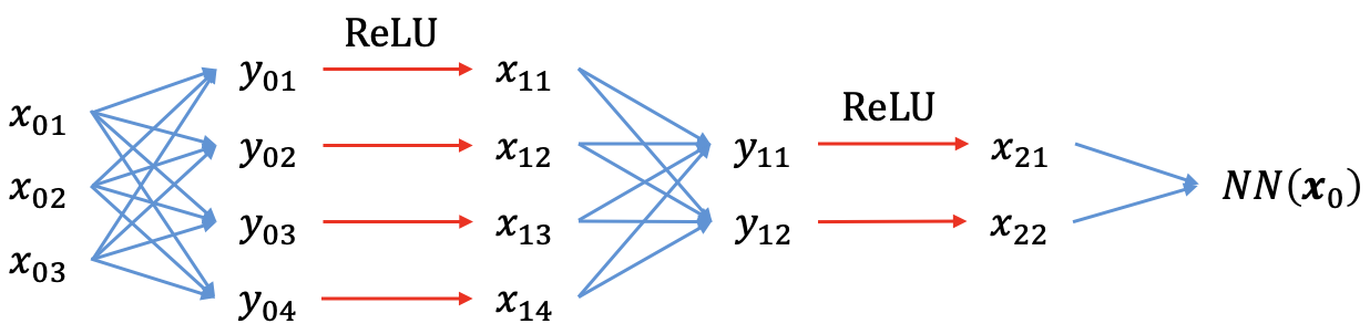
First, we introduce feed-forward neural networks (FNNs), a typical type of neural network. Here, we consider the Rectified Linear Unit (ReLU) activation function, which is defined as . FNNs take vectors as inputs and return real numbers as outputs. Strictly speaking, a ReLU FNN is defined as follows.
Definition 1 (ReLU feed-forward neural network).
Fix a number and , where . For the input , a ReLU FNN is a function which returns , which is described as follows: a sequence is defined by the recursive manner for :
where is defined as
Here, and are parameter matrices and bias vectors, respectively.
is referred to as the width of , and as its depth. The vectors are referred to as the hidden layers of . The vector is obtained by applying an affine transformation followed by the ReLU activation function to for . Note that the activation function is not applied when obtaining the final output from the last hidden layer . An example of a ReLU FNN is illustrated in Figure 1.
Next, we introduce the Transformer, an extension of the FNN. A Transformer receives matrices and returns matrices of the same size. It is constructed by repeatedly combining Transformer Blocks, each of which consists of two layers: an attention layer and a feed-forward layer. More precisely, we define the Transformer as follows:
Definition 2 (Transformer).
Fix . For any matrix , we define an attention layer with width and heads as
where are parameter matrices for . Here, the softmax function is applied column-wise: i.e. for a matrix , we define
where . Next, a feed-forward layer in a matrix form is defined
where are parameter matrices and are the bias vectors. Finally, a Transformer block is defined as
A function obtained by composing times is referred to as a Transformer network of width and depth .
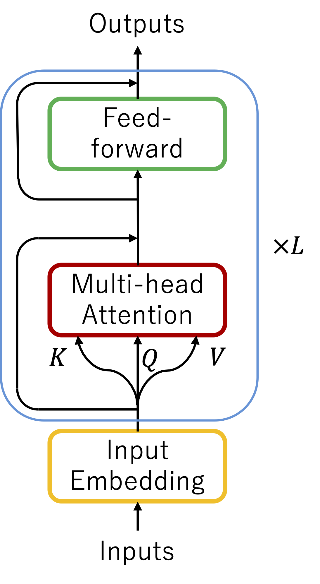
This definition omits layer normalization unlike Vaswani et al. (2017), for brevity. However, We denote that this does not affect the expressivity of the Transformer. Figure 2 illustrates the architecture of Transformers.
2.2. Symmetric Polynomials
In this section, we define symmetric polynomials where the input is a vector, and then consider the general case where the input is a matrix.
Definition 3.
A function is permutation invariant if holds for any permutation . In particular, if a polynomial with degree (the degree of the polynomial refers to the highest degree of the terms. e.g., the polynomial is a degree-3 polynomial.) is permutation invariant, we call it a symmetric degree- polynomial. For example, is a symmetric polynomial over . However, is not a symmetric polynomial as .
Next, we consider the matrix input case and define column-symmetric polynomials over matrices.
Definition 4.
A function with some is column permutation invariant if holds for any permutation . In particular, we call a column permutation invariant degree- polynomial as a column-symmetric degree- polynomial.
3. Universal Approximation of Column-Symmetric Polynomials
The main statement of this study demonstrates the relationship between the width and depth of the Transformer network and its approximation error. Since the approximating Transformer has only a single attention head, and its width and depth are independent of the number of input columns (denoted as ), the number of parameters is also independent of the number of input columns.
Theorem 1.
Let be an arbitrary degree- column-symmetric polynomial over with positive coefficients, satisfying : i.e. . Then, for any , there exists a 1-head Transformer network: with width at most , and depth at most , which satisfies
which has only a single attention head.
Since the coefficients in are positive, , the maximum value of in , is equal to , which is the sum of all coefficients appearing in . Hence, as long as the sum of the coefficients does not exceed an absolute constant, the approximation error remains independent of the number of rows and columns of the input matrix.
3.1. Examples
Here, we demonstrate some examples to make our main statement more familiar.
Example 1.
Let be the polynomial consisting of all terms of degree at most , with the coefficient of every term being equal to 1. For example, for the case when , is equivalent to
As the number of terms (terms can be written in the format of ) which appear in is at most the number of sets of integers which satisfy
it follows from Lemma 5 that the value of this equation is at most
implying . Thus, there exists a Transformer network with width at most , and depth at most , which approximates as
Example 2.
We consider the case when and
Since substituting with yields , there exists a Transformer network with width at most , and with depth at most , which approximates with an error of
By considering the average of all the terms in , the approximation error does not depend on the rows and columns of the input matrix.
4. Proof Outline
We present an outline of the proof of the main theorem. In preparation, we define the notation of an approximation error with a sign. For a function and a Transformer , we denote
as the signed approximation error of by at point . Note that this definition can be negative. the approximation error without a sign.
4.1. Monomial Column-symmetric Polynomials
We define a certain class of symmetric polynomials called monomial column-symmetric polynomials. These polynomials play a crucial role in our proof, as we approximate column-symmetric polynomials by taking a weighted sum of monomial column-symmetric polynomials.
In the case where , monomial column-symmetric polynomials coincide with monomial symmetric polynomials, which are defined as follows:
Definition 5 (Monomial symmetric polynomials).
A monomial symmetric polynomial is a symmetric polynomial which can be written as the sum of permutations of a single term. since and is a monomial symmetric polynomial over as are all permutations of . Similarly, is a monomial symmetric polynomial over .
Next, we consider the general case. For , we define a more complex polynomial by summing the column-permutations of a specific monomial. We provide its rigorous definition as follows:
Definition 6 (Monomial column-symmetric polynomials).
Fix and . We define a rank- monomial column-symmetric polynomials over as
In the case, the rank of monomial column-symmetric polynomials corresponds to the degree of the polynomial, as column-symmetric polynomials are equivalent to symmetric polynomials in this case. For the case of , the rank corresponds to the number of columns that each term spans.
We note that there are permutations in where are identical. Hence, is equivalent to the sum of , where are distinct. In addition, the coefficients of each term may not necessarily be equal to , as terms that become identical through permutations can be counted multiple times (e.g. and are permutations of the same monomial). For a monomial column-symmetric polynomial that includes the term , the corresponding coefficient is , where the tuple consists of occurrences of ’’, occurrences of ’’, , and occurrences of ’’, with being distinct. For example, when and , the tuple contains three ’1’s and two ’2’s, and hence .
We give several examples of the monomial column-symmetric polynomial.
Example 3.
For the case when , the rank- monomial column-symmetric polynomial is given by
In this case, the coefficients of the terms are all equal to 2. This is because the tuple has two ’’s.
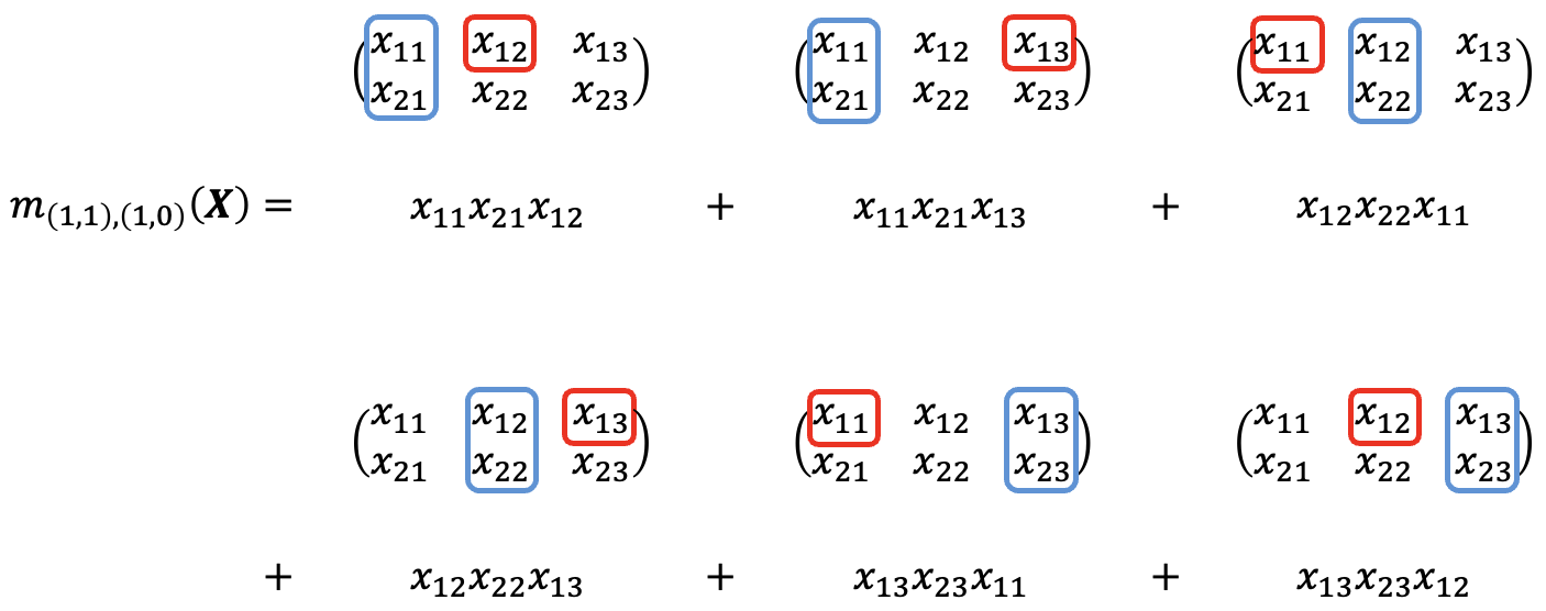
Example 4.
For the case when and the rank- monomial column-symmetric polynomial is given by
The following Figure 3 is a corresponding illustration.
4.2. Summary of the Proof of Theorem 1
From Section 5 to Section 8 below, we construct the approximation of in multiple steps, as illustrated in Table 1.
| Target of Approximation | Analysis | Layer used | ||
|---|---|---|---|---|
| Section 5.1 | Feed-forward | |||
| Section 5.2, 5.3 | Feed-forward | |||
|
Section 6 | Single-head Attention | ||
|
Section 7 | Feed-forward | ||
| Section 8 | Feed-forward |
First, we approximate multiplication, specifically for . By repeatedly applying this approximation, we can approximate column-wise monomials, such as . Using this method, we prove Proposition 1, which is demonstrated in Section 5.
Proposition 1.
There exists a feed-forward network (i.e. a Transformer network consisted only of feed-forward layers) , whose width is at most and depth at most , which approximates all monomials over , i.e.
Second, we take the column-wise sum of these approximations of monomials, obtaining approximations of rank- monomial column-symmetric polynomials. The following proposition is proved in Section 6.
Proposition 2.
There exists a single-attention Transformer network , whose width is at most and depth at most , which satisfies
where the approximation errors satisfy
Next, we construct monomial column-symmetric polynomials of higher rank by induction on the rank. This enables us to obtain the following proposition, which is proved in Section 7.
Proposition 3.
There exists a Transformer network with width at most and depth at most , such that
where
Finally, we approximate the column-symmetric polynomial by taking a weighted sum of monomial column-symmetric polynomials. The column-wise summation is performed by a single-head attention layer, while the other processes are conducted by the feed-forward layer.
5. Proof of Proposition 1
5.1. Approximating Products
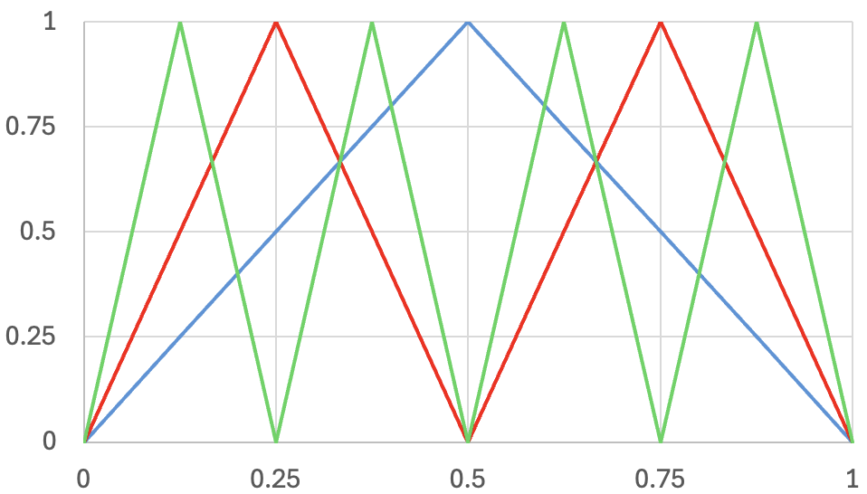
Here, we approximate the function by ReLU FNNs by the method used by Yarotsky (2017) and Lu et al. (2021). First, we approximate the function for . Let be
and . Then, becomes the sawtooth function illustrated in Figure 4.
As a result, the following statement holds, which will be proved in B.
Lemma 1.
The equality
holds for any and , where . In particular, holds for any .
Let be the integer satisfying . Then, from Lemma 7, it is easy to verify that is piecewise linear in the interval for . Hence, can be constructed by a ReLU FNN with width and depth . Note that the composition of a depth- ReLU FNN, , and a depth- ReLU FNN, , can be achieved with a depth- ReLU FNN, since obtaining the output of from its last hidden layer is merely an affine transformation, which can be combined with the first affine transformation of . As a result, can be approximated by the ReLU FNN illustrated in Figure 6, which has a width of at most and a depth of .
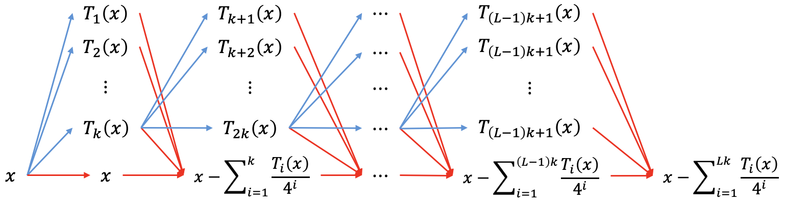
By considering that , the function is an approximation of , which can be approximated by a ReLU FNN with width at most , and depth at most , as illustrated in Figure 7. Combining this with the following lemma, can be approximated by a Transformer network with width at most , and depth at most . The proof is in C.
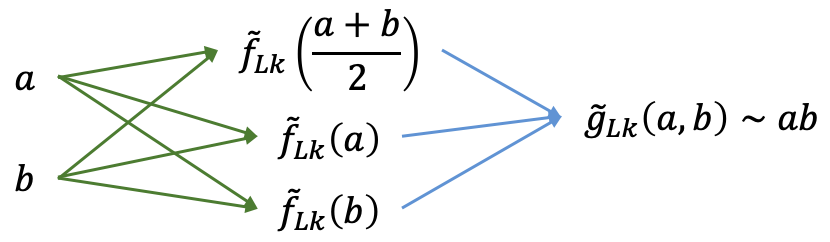
Lemma 2.
A ReLU FNN with width and depth , where all the values of inputs, outputs and hidden layers are all non-negative, can be constructed by a Transformer network with width and depth .
5.2. Approximation of Polynomials
We construct a neural network to approximate polynomials. Since constructed in Section 5.1 is convex and holds for any ,
holds for any . Hence, satisfies , and by applying repeatedly, we can obtain an approximation of . As degree mononomials of can be written in the format where , the total number of such polynomials is at most
This implies that the number of monomials of degree or less of are at most . Note that constructing a monomial of degree or less requires at most multiplications and has width and depth , due to the extra layer applying the ReLU function. By approximating all the single-term polynomials in , , the Transformer network approximating all monomials over with degree or less, can be constructed with width at most , and depth at most .
5.3. Approximation Error
We study an approximation error of the neural networks constrcuted above.
First, we evaluate the approximation error of . Since
and holds for all , the value of must be at least and be at most . Since we defined so that holds, we obtain
and for yields
Next, we discuss the approximation error of column-wise monomials. Specifically, we show that the approximation error of a degree- monomial of is at most , by induction.
The case for is obvious, because we do not need to take products. Assume the hypothesis is true for degree-. In this case, , the approximation error of by satisfies . And because , the approximation error of is at most
which completes the induction. Hence, the approximation error of by is at most , proving Proposition 2.
6. Proof of Proposition 2
Since feed-forward layers affect each columns independently,
| (1) |
holds: i.e. the monomials of are simultaneously produced in the th columns respectively. Let be the number of rows in . By setting in the attention layer, we obtain
where . Hence, if we define as the composition of and the above attention layer, equation (1) yields
since ( denotes the -th column of matrix ). Hence, we have constructed all the rank-1 monomial column-symmetric polynomials of , with degree or less. As is a composition of and a single-head attention layer, the width and depth of are at most and .
7. Proof of Proposition 3
From the following lemma, we can obtain rank- monomial column-symmetric polynomials from rank- and rank- monomial column-symmetric polynomials, by addition and multiplication.
Lemma 3.
For , the following equality holds:
| (2) |
Proof.
The lemma can be proved by multiplying a rank- monomial column-symmetric polynomial with a rank- monomial column-symmetric polynomial, and subtracting the extra terms. If ,
holds (note that the coefficient becomes in the second row, as the term
corresponds to the sum over elements in ). Next, if , then
implying that both sides of equation (2) are equal to 0. Last, if , both sides of equation 2 are equal to 0, since monomial column-symmetric polynomials with rank- or greater are all equal to 0 from its definition. ∎
Assume that a Transformer approximates all monomial column-symmetric polynomials with rank- or less. Now, we denote as the approximation of by . If and , we can approximate rank- monomial column-symmetric polynomials by
| (3) |
Thus, all monomial column-symmetric polynomials of rank- or less can be constructed inductively. In the remainder of this section, we evaluate the Transformer network that approximates monomial column-symmetric polynomials of higher ranks, given that the approximation of rank-1 column-symmetric polynomials is provided as input. We evaluate its size in Section 7.1 and its approximation error in Section 7.2.
7.1. Size of Transformer Network
By the result above, when the approximations of monomial column-symmetric polynomials of rank- or less are given as inputs, we can construct the right-hand side of equation (3) using a Transformer with width and depth , since applying requires such a size (note that addition, subtraction, and scaling of terms can be achieved by adjusting the parameter matrix in the final feed-forward layer). In addition, when constructing approximations of rank- monomial column-symmetric polynomials, we apply the functions and at the end to ensure that the values of the Transformer approximation of rank- monomial column-symmetric polynomials lie within the range . (note that the maximum value of rank- monomial column-symmetric polynomials is
as has elements). As a result, approximating monomial column-symmetric polynomials of rank- from those of ranks and can be achieved by a Transformer network with width and depth per polynomial.
Next, we consider the total number of monomial column-symmetric polynomials of rank-. Consider a rank- monomial column-symmetric polynomial containing the term . From Lemma 5, the possible combinations of is , as .
In addition, consider the total number of combinations of , where are fixed. For each , the number of solutions satisfying the equation with , by Lemma 5, is at most
Since the product over all -s yields , the total number of degree- monomial symmetric polynomials is at most . Hence, to construct a single degree- monomial column-symmetric polynomial from degree- monomial column-symmetric polynomials, the required width is at most
(note we have used Lemma 4 in the first inequality) and the depth is at most . Hence, can be realized with a Transformer network having width at most and depth at most .
7.2. Approximation Error
In this subsection, we will provide an upper bound of the approximation error of monomial column-symmetric polynomials by . We will prove by induction, based on Lemma 3.
According to Section 5.3, the approximation error of the rank-1 monomial column-symmetric polynomial was at most . Hence the assumption holds for . Next, assume that the approximation error of in is at most , for any such that . From equation (3), the approximation error of a rank- monomial column-symmetric polynomial is at most
as the approximation error of is at most in . Since the maximum values of and in are and , we obtain the the upper bound of the approximation error by performing some algebra, which is
| (4) |
Now, the approximation errors of and in by are at most and (the former follows from the assumption of the induction, and the latter from Section 5.3). Hence, the first 2 terms of equation (4) are at most
The next term in equation (4) is at most
From these inequalities, the first 3 terms in equation (4) is bounded by
In addition, by using the inequality for , the upper bound of the remaining terms in (4) (i.e. ) is
Hence, equation (4), the approximation error of in , is at most
which completes the induction. Thus, we have proved Proposition 3.
8. Combining Pieces to Prove Theorem 1
According to Section 7.2, the approximation error for the rank- column-monomial symmetric polynomial is at most
| (5) |
Note that when , the value of the weighted column-monomial symmetric polynomial becomes . Dividing the approximation error (5) by , we obtain
If , which is when the monomial column-symmetric polynomial is non-zero, and as long as is fixed, the terms monotonically decrease as gets larger. Hence, as , the formula above is bounded by
where the first inequality follows from the inequality for , implying the maximum of is achieved when and . Thus, we obtain the approximation error for weighted rank- monomial column-symmetric polynomials as
From Lemma 6, any permutation symmetric function can be expressed as a weighted sum of monomial symmetric polynomials: i.e. there exist coefficients such that
Thus, by taking the sum of all weighted monomial column-symmetric polynomials, we obtain the upper bound of the approximation error for as
Now, can be constructed by a Transformer network with width at most and depth at most . Since taking the weighted sum of inputs on the same column can be achieved by the feed-forward layer, can be constructed by altering the parameters of the last feed-forward layer of . Hence, we have proved Theorem 1.
9. Discussions
9.1. Transformer vs. Neural networks
In this paper, we have utilized the parameter efficiency of Transformers, specifically the efficiency of the attention layer and the parallel processing capability of the feed-forward layer. Since we used only the attention layer to compute the row-wise sum of inputs, the entire process in this paper can be implemented using neural networks by treating the input as a dimensional vector. However, in this case, it is difficult to fully reflect the symmetry of the target function in terms of parameter efficiency, as separate parameters are required to construct column-wise monomials (as described in Section 5) for each individual column in . Similarly, computing the sum of column-wise monomials (as described in Section 6) also requires individual parameters for each column in . As a result, the number of parameters needed to construct a neural network equivalent to (in Proposition 2) increases linearly with the number of input columns, whereas it remains constant in Transformers. Hence, our construction requires fewer parameters compared to conventional neural networks when holds.
9.2. Discussion on Number of Parameters
In this study, monomial column-symmetric polynomials were used to universally approximate column-symmetric polynomials using single-headed Transformers, whose number of parameters does not depend on the number of input columns. This coincides with previous work Kajitsuka and Sato (2024), which demonstrates that single-layer Transformers are universal approximators. Furthermore, the number of feed-forward layers required by the Transformer is approximately , which is comparable to the depth of Transformers used in practice.
In addition, when the degree of the target function is small, particularly when , the width of the Transformer can be of practical size. This corresponds to the case where the inputs interact with only a very limited number of other elements. In addition, the approximation error decreases exponentially with respect to the number of layers, while it only decreases polynomially with respect to the width. Hence, our results demonstrate the efficiency of deep Transformers.
On the other hand, the width of is proportional to , which becomes excessively large as and increase. This issue arises because the number of monomial column-symmetric polynomials of degree or less within a single column increases exponentially with . Reducing the number of parameters to a practical level is a critical direction for future work to better understand the representational power of Transformers.
9.3. Discussion on Positional Encoding
When applying Transformers to various tasks, it is common to use positional encodings, values that distinguish individual columns, as in Vaswani et al. (2017). The use of positional encoding allows for discussions on more general cases, where symmetry is present only among specific columns. A similar discussion has been conducted in the context of neural networks in Maron et al. (2019). Exploring the impact of positional encodings raises intriguing questions: the extent of parameters required for such constructions and the specific architectures of Transformers. We leave these questions for future work.
Acknowledgements
We would like to express our gratitude to Prof. Naoto Shiraishi and Prof. Koji Fukushima for fruitful comments and discussions. This study was supported by JSPS KAKENHI (24K02904), JST CREST (JPMJCR21D2), and JST FOREST (JPMJFR216I).
Appendix A Basic Mathematical Properties
Here, we provide basic lemmas which are used in this paper.
Lemma 4.
For any , the following equation holds.
Hence, holds for any .
Lemma 4 easily follows from the binomial theorem, and from when . The following lemma is a well-known result of classic combinatorics.
Lemma 5.
The number of sets of integers which satisfy
are .
Proof.
Let . Then, the number of sets of integers are equivalent to the number of sets of integers which satisfy
As this is equivalent to choosing distinct integers from 1 to , the desired count is . ∎
Note that when the condition in Lemma 5 is altered to , by introducing an additional variable , the problem can be reformulated as finding the total number of non-negative integer solutions to , which is .
The next lemma demonstrates that monomial column-symmetric polynomials generate the set of column-symmetric polynomials.
Lemma 6.
Any column-symmetric polynomial can be written in a linear combination of monomial column-symmetric polynomials.
Proof.
First, we compare the degree of polynomials and . If , we regard has a higher degree than , and vice versa. If , we compare and and so on, similarly to the case of comparing vectors.
Let be the monomial in with the highest degree. In this case, for any permutation of , must have a lower degree than , since is column-symmetric and must contain these terms. Consider the polynomial
| (6) |
where is set so that the coefficient of in (6) is equal to 0. In this case, (6) must have a degree lower than that of , because otherwise it would contradict the assumption that has the largest degree.
By repeatedly applying this operation, eventually we arrive at a polynomial of degree 0, which is a constant. Thus, must be able to be expressed as a linear combination of monomial column-symmetric polynomials. ∎
Appendix B Proof of Lemma 1
Lemma 7.
The equality
holds for any and , where .
Proof.
We prove the lemma by induction on . The case for is trivial, since implies for any . Next, we assume Lemma 7 holds for . Since , we can divide the discussion into two cases.
First, if , then implies
resulting in .
Second, if , then implies
It is obvious that holds for any , so we obtain
In either case, we get , where and , which completes the induction. ∎
Now we can prove Lemma 1.
Proof.
We also prove this proposition by induction on . The case for is easy because
If Lemma 1 holds for , the assumption and Lemma 7 imply
Hence, if , then implies
On the other hand, if , then implies
For either case, holds for , where , completing the induction. The latter statement of Lemma 1 easily follows by completing the square. ∎
Appendix C Proof of Lemma 2
Assume that the ReLU FNN with width and depth can be written as
where and are the inputs and the output respectively. Without loss of generality, we can assume that the dimension of are equal to by adding 0s to each bottom. Let , and define
It is easy to check that the top elements of are equal to , and constructing for can be done by the feed-forward layers of Transformers.
References
- Bhojanapalli et al. (2020) Srinadh Bhojanapalli, Chulhee Yun, Ankit Singh Rawat, Sashank Reddi, and Sanjiv Kumar. Low-rank bottleneck in multi-head attention models. In International Conference on Machine Learning, pages 864–873. PMLR, 2020.
- Brown et al. (2020) Tom Brown, Benjamin Mann, Nick Ryder, Melanie Subbiah, Jared D Kaplan, Prafulla Dhariwal, Arvind Neelakantan, Pranav Shyam, Girish Sastry, Amanda Askell, Sandhini Agarwal, Ariel Herbert-Voss, Gretchen Krueger, Tom Henighan, Rewon Child, Aditya Ramesh, Daniel Ziegler, Jeffrey Wu, Clemens Winter, Chris Hesse, Mark Chen, Eric Sigler, Mateusz Litwin, Scott Gray, Benjamin Chess, Jack Clark, Christopher Berner, Sam McCandlish, Alec Radford, Ilya Sutskever, and Dario Amodei. Language models are few-shot learners. Advances in Neural Information Processing Systems, 33:1877–1901, 2020.
- Chen et al. (2019) Minshuo Chen, Haoming Jiang, Wenjing Liao, and Tuo Zhao. Efficient approximation of deep relu networks for functions on low dimensional manifolds. Advances in neural information processing systems, 32, 2019.
- Cybenko (1989) George Cybenko. Approximation by superpositions of a sigmoidal function. Mathematics of Control, Signals and Systems, 2(4):303â314, 1989.
- Devlin et al. (2018) Jacob Devlin, Ming-Wei Chang, Kenton Lee, and Kristina Toutanova. Bert: Pre-training of deep bidirectional transformers for language understanding. arXiv preprint arXiv:1810.04805, 2018.
- Dosovitskiy et al. (2021) Alexey Dosovitskiy, Lucas Beyer, Alexander Kolesnikov, Dirk Weissenborn, Xiaohua Zhai, Thomas Unterthiner, Mostafa Dehghani, Matthias Minderer, Georg Heigold, Sylvain Gelly, Jakob Uszkoreit, and Neil Houlsby. An image is worth 16x16 words: Transformers for image recognition at scale. In International Conference on Learning Representations, 2021.
- Goldberg and Jerrum (1993) Paul Goldberg and Mark Jerrum. Bounding the vapnik-chervonenkis dimension of concept classes parameterized by real numbers. In Proceedings of the Sixth Annual Conference on Computational Learning Theory, pages 361–369, 1993.
- Hayakawa and Suzuki (2020) Satoshi Hayakawa and Taiji Suzuki. On the minimax optimality and superiority of deep neural network learning over sparse parameter spaces. Neural Networks, 123:343–361, 2020.
- Hornik (1991) Kurt Hornik. Approximation capabilities of multilayer feedforward networks. Neural Networks, 4 (2):251â257, 1991.
- Imaizumi and Fukumizu (2019) Masaaki Imaizumi and Kenji Fukumizu. Deep neural networks learn non-smooth functions effectively. Proceedings of Machine Learning Research (International Conference on Artificial Intelligence and Statistics), 2019.
- Imaizumi and Fukumizu (2022) Masaaki Imaizumi and Kenji Fukumizu. Advantage of deep neural networks for estimating functions with singularity on hypersurfaces. Journal of Machine Learning Research, 23(111):1–54, 2022.
- Kajitsuka and Sato (2024) Tokio Kajitsuka and Issei Sato. Are transformers with one layer self-attention using low-rank weight matrices universal approximators? In International Conference on Learning Representations, 2024.
- Kim et al. (2023) Junghwan Kim, Michelle Kim, and Barzan Mozafari. Provable memorization capacity of transformers. In International Conference on Learning Representations, 2023.
- Kratsios et al. (2022) Anastasis Kratsios, Behnoosh Zamanlooy, Tianlin Liu, and Ivan Dokmanić. Universal approximation under constraints is possible with transformers. In International Conference on Learning Representations, 2022.
- Likhosherstov et al. (2021) Valerii Likhosherstov, Krzysztof Choromanski, and Adrian Weller. On the expressive power of self-attention matrices. arXiv preprint arXiv:2106.03764, 2021.
- Lu et al. (2021) Jianfeng Lu, Zuowei Shen, Haizhao Yang, and Shijun Zhang. Deep network approximation for smooth functions. SIAM Journal on Mathematical Analysis, 53(5):5465–5506, 2021.
- Lu et al. (2017) Zhou Lu, Hongming Pu, Feicheng Wang, Zhiqiang Hu, and Liwei Wang. The expressive power of neural networks: A view from the width. Advances in Neural Information Processing Systems, 30, 2017.
- Maron et al. (2019) Haggai Maron, Ethan Fetaya, Nimrod Segol, and Yaron Lipman. On the universality of invariant networks. In International Conference on Machine Learning, pages 4363–4371, 2019.
- Nakada and Imaizumi (2020) Ryumei Nakada and Masaaki Imaizumi. Adaptive approximation and generalization of deep neural network with intrinsic dimensionality. Journal of Machine Learning Research, 21(174):1–38, 2020.
- Park et al. (2021) Sejun Park, Jaeho Lee, Chulhee Yun, and Jinwoo Shin. Provable memorization via deep neural networks using sub-linear parameters. In Conference on Learning Theory, pages 3627–3661, 2021.
- Petersen and Voigtlaender (2018) Philipp Petersen and Felix Voigtlaender. Optimal approximation of piecewise smooth functions using deep relu neural networks. Neural Networks, 108:296–330, 2018.
- Sannai et al. (2019) Akiyoshi Sannai, Yuuki Takai, and Matthieu Cordonnier. Universal approximations of permutation invariant/equivariant functions by deep neural networks. arXiv preprint arXiv:1903.01939, 2019.
- Schmidt-Hieber (2020) Johannes Schmidt-Hieber. Nonparametric regression using deep neural networks with relu activation function. Annals of Statistics, 48(4):1875–1897, 2020.
- Suzuki (2019) Taiji Suzuki. Adaptivity of deep relu network for learning in besov and mixed smooth besov spaces: optimal rate and curse of dimensionality. International Conference on Learning Representation, 2019.
- Takakura and Suzuki (2023) Shokichi Takakura and Taiji Suzuki. Approximation and estimation ability of transformers for sequence-to-sequence functions with infinite dimensional input. pages 33416–33447, 2023.
- Vardi et al. (2022) Gal Vardi, Gilad Yehudai, and Ohad Shamir. On the optimal memorization power of ReLU neural networks. In International Conference on Learning Representations, 2022.
- Vaswani et al. (2017) Ashish Vaswani, Noam Shazeer, Niki Parmar, Jakob Uszkoreit, Llion Jones, Aidan N Gomez, Ł ukasz Kaiser, and Illia Polosukhin. Attention is all you need. Advances in Neural Information Processing Systems, 2017.
- Yarotsky (2017) Dmitry Yarotsky. Error bounds for approximations with deep ReLU networks. Neural networks, 94:103–114, 2017.
- Yarotsky (2022) Dmitry Yarotsky. Universal approximations of invariant maps by neural networks. Constructive Approximation, 55(1):407–474, 2022.
- Yun et al. (2019) Chulhee Yun, Srinadh Bhojanapalli, Ankit Singh Rawat, Sashank Reddi, and Sanjiv Kumar. Are transformers universal approximators of sequence-to-sequence functions? In International Conference on Learning Representations, 2019.
- Yun et al. (2020) Chulhee Yun, Yin-Wen Chang, Srinadh Bhojanapalli, Ankit Singh Rawat, Sashank Reddi, and Sanjiv Kumar. O (n) connections are expressive enough: Universal approximability of sparse transformers. Advances in Neural Information Processing Systems, 33:13783–13794, 2020.
- Zaheer et al. (2017) Manzil Zaheer, Satwik Kottur, Siamak Ravanbakhsh, Barnabas Poczos, Russ R Salakhutdinov, and Alexander J Smola. Deep sets. Advances in neural information processing systems, 30, 2017.
- Zaheer et al. (2020) Manzil Zaheer, Guru Guruganesh, Kumar Avinava Dubey, Joshua Ainslie, Chris Alberti, Santiago Ontanon, Philip Pham, Anirudh Ravula, Qifan Wang, Li Yang, et al. Big bird: Transformers for longer sequences. Advances in neural information processing systems, 33:17283–17297, 2020.