Fishing For Cheap And Efficient Pruners At Initialization

Abstract

Pruning offers a promising solution to mitigate the associated costs and environmental impact of deploying large deep neural networks (DNNs). Traditional approaches rely on computationally expensive trained models or time-consuming iterative prune-retrain cycles, undermining their utility in resource-constrained settings. To address this issue, we build upon the established principles of saliency (LeCun et al., 1989) and connection sensitivity (Lee et al., 2018) to tackle the challenging problem of one-shot pruning neural networks (NNs) before training (PBT) at initialization. We introduce Fisher-Taylor Sensitivity (FTS), a computationally cheap and efficient pruning criterion based on the empirical Fisher Information Matrix (FIM) diagonal, offering a viable alternative for integrating first- and second-order information to identify a model’s structurally important parameters. Although the FIM-Hessian equivalency only holds for convergent models that maximize the likelihood, recent studies (Karakida et al., 2019) suggest that, even at initialization, the FIM captures essential geometric information of parameters in overparameterized NNs, providing the basis for our method. Finally, we demonstrate empirically that layer collapse, a critical limitation of data-dependent pruning methodologies, is easily overcome by pruning within a single training epoch after initialization. We perform experiments on ResNet18 and VGG19 with CIFAR-10 and CIFAR-100, widely used benchmarks in pruning research. Our method achieves competitive performance against state-of-the-art techniques for one-shot PBT, even under extreme sparsity conditions. Our code is made available to the public.

1 Introduction

We hear of breakthroughs daily thanks to Artificial Intelligence (AI) systems. The exponential increase in computing power and data availability has allowed success stories in robotics (Soori et al., 2023), computer vision (Khan & Al-Habsi, 2020), natural language processing (Torfi et al., 2020), healthcare (Habehh & Gohel, 2021), and many other fields. Naturally, new challenges have emerged alongside this progress, particularly the growing size of AI systems and the associated high training and inference costs (Han et al., 2015). The “bigger is better” approach goes against real-life applications that require high accuracy and efficient resource usage. Furthermore, climate change awareness highlights the environmental impact of AI, with inference being a significant contributor to model-associated carbon emissions (Wu et al., 2022; Chien et al., 2023). In addition, computational resources, energy, and bandwidth limit the deployment of large systems on edge devices (Cheng et al., 2024).

To overcome these challenges, researchers have developed techniques to address the constantly growing model sizes and associated costs of Deep Neural Networks (DNNs). The most prominent are quantization (Dettmers et al., 2023), low-rank factorization (Denton et al., 2014), knowledge distillation (Xu et al., 2024), neural architecture search (Zhang et al., 2021), and neural network pruning (Cheng et al., 2024). The latest stands out for its ability to dramatically decrease the model size, reducing storage memory for models and computation workload during training or inference while maintaining performance compared to the original network. Cheng et al. (2024) proposed a comprehensive taxonomy highlighting different aspects to consider in existing pruning techniques based on three questions: (1) Does the method achieve universal or specific acceleration through neural network pruning? (2) When does the pruning happen in the training pipeline? and (3) Is there a predefined pruning criterion, or is it learnable?

Regardless of the kind of acceleration or criterion, pruning after training (PAT) methods are investigated more frequently given the advantage of working with converged models, which implies parameters whose values are close to optimal and provide more information than randomly initialized ones (Kumar et al., 2024). A simple but very effective strategy explored by Han et al. (2015) involves masking (setting to zero) parameters whose magnitudes are below a given threshold. The removal of a fraction of unimportant connections reduces operations and accelerates inference. More principled approaches utilize first-order and/or second-order information to measure the loss change induced by pruning low-information parameters (LeCun et al., 1989; Hassibi & Stork, 1992).

The advantages of PAT come at the expense of training a fully dense network and the required post-finetuning and/or readjustment of parameters. Consequently, there is an active interest in the research community in performing pruning during (PDT) or before (PBT) training. The milestone work of Frankle & Carbin (2018) empirically showed the existence of sparse subnetworks or “winning tickets” that match or even surpass the performance of the dense model utilizing the same parameter initialization as the dense network. Their algorithm iteratively prunes and rewinds the network parameters to uncover these subnetworks. Since then, there has been an effort to find efficient subnetworks quicker to reduce expensive prune-retrain cycles (Sreenivasan et al., 2022; You et al., 2022), or at initialization pioneered by Lee et al. (2018).

We take inspiration from classical (LeCun et al., 1989; Hassibi & Stork, 1992) and modern (Lee et al., 2018; Singh & Alistarh, 2020) techniques and introduce Fisher-Taylor Sensitivity (FTS), a pruning criterion to operate in the challenging one-shot PBT setting, where performant subnetworks must be identified in a single step at initialization to minimize computation overhead. Our approach approximates the objective function using a Taylor expansion to measure the sensitivity of parameters at initialization. In addition, we employ the Fisher Information Matrix (FIM) diagonal for a computationally cheap and efficient approximation of second-order information, enabling the discovery of performant subnetworks before the training process. The role of the FIM in pruning at initialization remains poorly explored, given that the FIM is often connected to the Hessian only in converged models. However, the work by Karakida et al. (2019) suggests that this relationship might extend to initialization in overparameterized networks. Therefore, FIM provides useful structural information about the importance of parameters for pruning, even at initialization. Using this insight, we also introduce a batched gradient-based estimation of the FIM diagonal, which improves approximation quality while reducing computational overhead.

Recent works (Tanaka et al., 2020; Kumar et al., 2024) have elaborated on the limitations of pruning at initialization. A key challenge for data-dependent pruning criteria is layer collapse. This failure mode occurs when an entire layer (or most of its parameters) is pruned, disrupting the information flow across subsequent layers. This effect renders the network untrainable, as the pruned layer creates a bottleneck that hinders the model’s learning ability. Since data-dependent methods rely on gradient-based information, they tend to assign disproportionately low scores to wide layers, causing them to be pruned first, ultimately collapsing the network.

Considering that layer collapse occurs when pruning at initialization, allowing the gradients to align during a brief warmup phase proves to be a simple yet effective strategy to overcome this issue. Specifically, we find in our experiments that a single warmup epoch mitigates layer collapse. This step ensures that the information flow is not interrupted and enables successful training of the pruned network.

We evaluated the proposed criterion with architectures widely studied in the pruning literature. Specifically, ResNet18 (He et al., 2016) and VGG19 (Simonyan, 2014). We used the CIFAR-10 and CIFAR-100 datasets (Krizhevsky et al., 2009) to rigorously assess the robustness of our proposed pruning criterion in diverse data distributions and model structures. FTS consistently outperforms or matches state-of-the-art techniques for the one-shot PBT setting, even at extreme sparsity conditions. In summary, our key contributions are as follows:

1. We propose FTS, a novel pruning criterion that integrates first and second-order information for effective one-shot PBT.

2. We demonstrate the advantage of a batched gradient approach for estimating the FIM diagonal, reducing the approximation variance and computational overhead.

3. We demonstrate that a single warmup epoch mitigates layer collapse, ensuring stable pruned network training.

4. We achieve superior or competitive performance compared to state-of-the-art one-shot PBT methods across ResNet18 and VGG19 on CIFAR-10 and CIFAR-100, even under extreme sparsity.

2 Background

Problem Setting. This research focuses on unstructured pruning techniques in a supervised learning setting. Thus, we assume access to the training set $\mathcal{D}=\{(x_{n},y_{n})\}_{n=1}^{N}$, composed of tuples of input $x_{n}\in\mathcal{X}$ and output $y_{n}\in\mathcal{Y}$. The goal is to learn a model parameterized by $w\in\mathbb{R}^{d}$ that maps $f:\mathcal{X}\rightarrow\mathcal{Y}$ by minimizing an objective function:

$$\mathcal{L}(w)=\frac{1}{N}\sum_{n=1}^{N}l(y_{n},f(x_{n};w)).$$ (1)

A binary mask $m\in\{0,1\}^{d}$ is introduced to selectively prune the weights, effectively reducing the parameter count of the model. The pruned model is defined as $f(x_{n};m\odot w)$, where $\odot$ represents the Hadamard product between the mask $m$ and the model weights $w$. Thus, the objective function for training the pruned model becomes as follows:

$$\mathcal{L}(m\odot w)=\frac{1}{N}\sum_{n=1}^{N}l(y_{n},f(x_{n};m\odot w)).$$ (2)

where $m$ is constructed with the help of a pruning criterion and the percentage of pruned weights the user selects. Training a pruned model allows for a decrease in the model size, reducing storage memory and computation workload while maintaining performance compared to the original network. We use $q\in\mathcal{Q}$, with $\mathcal{Q}=\{1,2,\dots,d\}$, as an index to refer to an element $w_{q}$ in parameter vector $w$.

Classical PAT Methods. Pruning methods have been of interest to the research community even before the existence of the large models widely used today (which extend memory constraints due to their composition of billions of parameters). The cornerstone work of LeCun et al. (1989) motivated the removal of irrelevant parameters to improve generalization and inference speed in a PAT setting. The importance of parameters is defined by the saliency, a measurement of how much the objective function changes when a parameter is removed. As individually removing a parameter and reevaluating the objective function is unfeasible (in a reasonable time), they presented optimal brain damage (OBD), a method that utilizes a second-order Taylor series to evaluate saliency analytically under three assumptions: (1) the computationally expensive Hessian matrix $H$ is approximated using only its diagonal, which is more tractable; (2) assuming a converged model, the first-order term of the Taylor series is negligible; and (3) the local error model is assumed quadratic, so the higher-order components are discarded. Leading to an expression of saliency for a parameter $q$ given by:

$$s_{q}=\frac{1}{2}w_{q}^{2}H_{qq}.$$ (3)

A few years later, (Hassibi & Stork, 1992) revisited the approach and proposed Optimal Brain Surgeon (OBS). They highlighted the importance of a more complete representation of second-order information that includes off-diagonal elements and criticized the need to fine-tune the subnetwork. They redefined (3) as a constrained optimization:

$$\min_{q\in\mathcal{Q}}\min_{\delta w\in\mathbb{R}^{d}}\left\{\frac{1}{2}\delta w^{\top}H\delta w~~~\text{s.t.}~~~e_{q}^{\top}\delta w+w_{q}=0\right\},$$ (4)

where $e_{q}$ is a one-hot vector corresponding to $w_{q}$. Solving (4) leads to finding unimportant parameters that can be removed. Forming a Lagrangian, they derived a general expression for the saliency that includes (3) as a special case, and an expression to recalculate the magnitude of all parameters after removing a parameter $q$ to avoid fine-tuning the subnetwork. We include the intermediate steps for the reader in the Appendix A.

$$\delta w=-\frac{w_{q}H^{-1}e_{q}}{[H^{-1}]_{qq}},~~~ ~~~s_{q}=\frac{w_{q}^{2}}{2[H^{-1}]_{qq}}.$$ (5)

Furthermore, they introduced a process to compute the inverse of the Hessian matrix $H^{-1}$ efficiently through outer product approximation and the Woodbury matrix identity in its Kailath variant. Their main contributions rely on using a more accurate second-order estimation and $\delta w$ as a rescaling factor while pruning, making fine-tuning after pruning optional.

Fisher Information Matrix. Despite the demonstrated effectiveness of leveraging second-order information in pruning methodologies, the computational cost of calculating and storing the Hessian limits its application on NNs composed of millions or even billions of parameters. This has led to exploring inexpensive alternatives to estimate second-order information, such as the Fisher Information Matrix (FIM) (Vacar et al., 2011). By definition, the FIM captures the sensitivity of the model parameters $w$ with respect to the likelihood function $p(y\mid x,w)$, which describes the probability of observing the output $y$ given the input $x$ and the parameters $w$. Formally, the FIM is the expectation, with respect to the data distribution, of the second moment of the score function or the gradient of the log-likelihood:

$$F(w)=\mathbb{E}\left[\nabla\log p(y\mid x,w)\nabla\log p(y\mid x,w)^{\top}\right].$$ (6)

Assuming regularity conditions (Schervish, 2012), we can express the FIM in terms of the Hessian of the log-likelihood. Relying on the probabilistic concept that minimizing the loss function $l(y,f(x;w)$ is the equivalent of maximizing the negative log-likelihood $-\log p(y\mid x,w)$, the connection between the FIM and the Hessian is defined as:

(7)

Still, the size of the Fisher Information Matrix (FIM) is proportional to $\mathbb{R}^{d\times d}$, making it computationally prohibitive to calculate for modern NNs. Recently, Soen & Sun (2024) elaborated on the trade-offs of approximating the FIM only by its diagonal to reduce its computational complexity to $\mathbb{R}^{d}$. In practical settings, (6) is approximated using the empirical training distribution for an unbiased plug-in estimator, allowing the diagonal approximation to retain much of the relevant geometric information while significantly reducing computational complexity. This leads to the common formulation for the empirical FIM diagonal:

$$\hat{F}=\hat{F}(w) =\frac{1}{N}\sum_{n=1}^{N}\nabla l(y_{n},f(x_{n};w))^{2}.$$ (8)

This approximation has an intuitive interpretation: a given entry in $\hat{F}(w)$ corresponds to the average of the squared gradient of the model’s output with respect to a parameter. The parameters influencing the model’s output have larger entries, indicating higher importance. As this approach is computationally more efficient for calculating and retaining second-order information, it became a common approach in the pruning research space.

PAT Methods Based on the FIM. Theis et al. (2018) proposed using empirical FIM to approximate the Hessian in the PAT setting for the first time. As in OBD saliency (3), the first term vanishes (in practice, they found that including the first term reduced the performance of the pruning method), and the FIM diagonal is used to approximate the Hessian diagonal. Their saliency metric is defined as:

$$s_{q}=\frac{1}{2}w_{q}^{2}F_{qq},$$ (9)

Using a similar approach for structured pruning, Liu et al. (2021) employed Fisher information to estimate the importance of channels identified by a layer grouping algorithm that exploits the network computation graph. Layers in the same group have the same pruning mask computed using the FIM diagonal.

Inspired by OBS, Singh & Alistarh (2020) identified the challenges of computing and storing the inverse of the Hessian for large models and proposed a blockwise method to compute iteratively. The authors empirically showed the relationship between the empirical FIM inverse $\hat{F}^{-1}$ and Hessian inverse $H^{-1}$, concluding that as long as the application is scale-invariant, the first is a good approximation of the second. Furthermore, they compared their blockwise method with common alternatives to compute $\hat{F}^{-1}$.

PBT Methods. When referring to methods that prune at initialization time, it is necessary to mention the Lottery Ticket Hypothesis introduced by Frankle & Carbin (2018): “A randomly-initialized, dense neural network contains a subnetwork (winning ticket) that is initialized such that—when trained in isolation—it can match the test accuracy of the original network after training for at most the same number of iterations.” Effective training depends heavily on the parameter initialization, hence the comparison to a lottery. Certain initializations enable the discovery of subnetworks that can be dramatically smaller than the dense original network and reach or exceed its performance. The authors supported their hypothesis with an iterative pruning approach that consistently found performant Resnet-18 and VGG-19 subnetworks with compression rates of $80-90\%$ for a classification task (CIFAR-10). The importance of this work relies on introducing the existence of the winning tickets. However, they required a computationally expensive process, opening the question: If winning tickets exist, can we find them inexpensively?

Lee et al. (2018) tried to answer that question with a single-shot network pruning method called SNIP, which measures the connection sensitivity to perform PBT. They offered a different point of view on pruning, introducing an auxiliary vector of indicator variables $c\in\{0,1\}^{d}$ that defines whether a connection is active or not, turning the pruning into a Hadamard product between $c$ and the parameters $w$. From that point of view, the method focuses on the influence of a connection on the loss function, named $\Delta\mathcal{L}_{q}$, approximating it as a directional derivative $g_{q}(w;\mathcal{D})$ that represents the effect of perturbation $c_{q}$.

$$\Delta\mathcal{L}_{q}(w) =\lim_{\epsilon\rightarrow 0}\frac{\mathcal{L}(c\odot w)-\mathcal{L}((c-\epsilon e_{q})\odot w)}{\epsilon}\Bigg{\rvert}_{c=\mathbbm{1}},$$

$$=w_{q}\frac{\partial\mathcal{L}(w)}{\partial c_{q}}=g_{q}(w).$$ (10)

The intuition behind their proposed approach is that in PBT, the magnitude of the gradients with respect to the auxiliary vector $c$ indicates how each connection affects the loss, regardless of the direction. Allowing them to define their expression for the connection sensitivity as follows:

$$s_{q}=\frac{|g_{q}(c\odot w)|}{\sum_{k=1}^{m}|g_{k}(c\odot w)|}$$ (11)

Wang et al. (2020) claimed that effective training requires preserving gradient flow through the model. They proposed a method that heavily relies on the concept of Neural Tangent Kernel (NTK) (Jacot et al., 2018), which provides the notion of how the updates in a specific parameter affect the others throughout the training process. By defining the gradient flow as the inner product $\nabla\mathcal{L}(w)^{\top}\nabla\mathcal{L}(w)$ they found a link to the NTK through its eigendecomposition, claiming that their method Gradient Signal Preservation (GraSP) helps to select the parameters that encourage the NTK to be large in the direction corresponding to the output space gradients. In a similar fashion, they proposed a sensitivity metric that measures the response to a stimuli $\delta$.

$$S(\delta) =\Delta\mathcal{L}(w_{0}+\delta)-\Delta\mathcal{L}(w_{0})$$

$$=2\delta^{\top}H\nabla\mathcal{L}(w)+\mathcal{O}(||\delta||_{2}^{2})$$ (12)

Tanaka et al. (2020) proposed a data-agnostic approach named SynFlow. Their pruning method is designed to identify sparse and trainable subnetworks within NNs at their initialization without the need for training data. Previous methods require gradient information from the data and can inadvertently induce layer collapse, rendering the network untrainable due to information flow interruption. SynFlow addresses this by iteratively preserving the total “synaptic flow,” or the cumulative strength of the connections, throughout the network during pruning. This approach ensures that essential pathways remain intact, maintaining the network’s trainability.

3 Methodology

FIM at initialization. The equivalence between FIM and Hessian described in (7) only holds when the parameter vector $w$ is well specified. In other words, $w$ maximizes the likelihood $\mathbb{E}[\nabla\log p(y\mid x,w)]=0$. However, with randomly initialized parameters, the FIM-Hessian equivalence does not hold. Despite this, we argue that the FIM remains a valuable approximation for second-order information at initialization. Our claim is based on the findings of Karakida et al. (2019) for FIM in overparameterized DNNs with randomly initialized weights and large width limits. They demonstrate that even at initialization, the FIM captures essential geometric properties of the parameter space. Their study revealed that while most FIM eigenvalues are close to zero and indicate local flatness, a few are significantly large and induce strong distortions in certain directions. This suggests that even at initialization, the FIM could offer a notion of the parameters that significantly perturb the objective function, in other words, the sensitivity. This is an important attribute as we claim that in the PBT setting, we would rather preserve connections with the potential of impacting the likelihood of the model.

Fisher-Taylor Sensitivity. Considering the effectiveness of the saliency metric in identifying important parameters for preservation during pruning operation, the natural extension is to adjust the measurement for pruning at different training points. We follow OBD (LeCun et al., 1989) and approximate the objective function $\mathcal{L}$ using a Taylor series, where a perturbation $\delta w$ of the parameter vector will change $\mathcal{L}$ by

$$\delta\mathcal{L} =\mathcal{L}(w)-\mathcal{L}(w+\delta w),$$

$$=\delta w^{T}\nabla\mathcal{L}(w)+\frac{1}{2}\delta w^{T}H\delta w+\mathcal{O}(||\delta w||^{3}).$$ (13)

Since our goal is to prune at the initialization, neglecting the first-order term is not viable as the model parameters are not yet optimized. Still, we operate assuming that the local error is quadratic to discard higher-order components. However, the perturbation model in (13) still faces the high computational cost of computing the Hessian. Additionally, we cannot ensure that it is positive semidefinite (PSD) for randomly initialized weights. This leads to misleading evaluations of parameter importance, as negative eigenvalues in the Hessian may suggest the presence of saddle points or non-convex regions.

To address the computational cost of computing the Hessian, we replace it with the FIM, a cheap and efficient approximation of the second-order information. The FIM has the desirable property of being PSD by construction, ensuring a stable representation of the importance of the parameters. We further simplify the approximation using the FIM diagonal. This approach assumes that the sum of $\delta\mathcal{L}$ if the parameters are deleted individually equals the change in $\delta\mathcal{L}$ if the parameters are removed simultaneously. Substituting the FIM diagonal into (13), the Taylor series approximation becomes:

$$\delta\mathcal{L}=\sum_{q\in\mathcal{Q}}\delta w_{q}\frac{\partial\mathcal{L}(w)}{\partial w_{q}}+\frac{1}{2}\sum_{q\in\mathcal{Q}}\delta w_{q}^{2}\hat{F}_{qq},$$ (14)

Our interest is to discover important parameters in the model for one-shot pruning at initialization. We consider the term sensitivity more suitable than saliency for our setting because induced perturbations will cause $\mathcal{L}$ to increase, decrease, or stay the same, unlike pruning a converged model where perturbation only increases or preserves $\mathcal{L}$. Therefore, we take the magnitude of (14) as our sensitivity criterion. Note that a high magnitude means that the parameter $w_{q}$ significantly changes the objective function (either positive or negative), and it must be preserved for the pruned model to learn. Based on this, we define Fisher-Taylor Sensitivity (FTS) as our score of parameter importance:

$$s_{q}=\left|w_{q}\frac{\partial\mathcal{L}(w)}{\partial w_{q}}+\frac{1}{2}w_{q}^{2}\hat{F}_{qq}\right|.$$ (15)

Batch-wise FIM Estimation. In practice, we take advantage of the additive properties of the empirical FIM and approximate it by aggregating the squared gradients of individual data points in the training set $\mathcal{D}$, as seen in Equation (8). However, aggregation of single-sample gradients, especially at initialization, introduces high variance in the approximation. To mitigate this, we evaluated splitting $\mathcal{D}$ into $B$ batches, with $B\in\mathcal{B}$ and $\mathcal{B}=\{B^{k}\}_{k=1}^{B}$, to compute a more stable approximation with the averaging gradients while reducing computational overhead. This leads to the following batch-wise approximation of the FIM:

$$\hat{F}(w)\approx\frac{1}{B}\sum_{k=1}^{B}\text{diag}\left(\nabla\mathcal{L}_{B^{k}}(w)\nabla\mathcal{L}_{B^{k}}(w)^{\top}\right).$$ (16)

Pruning Mask. Given a partition of the data set, we compute and accumulate the gradients in vector $\tilde{g}$ and the diagonal entries of the FIM in vector $d_{F}$. Then, we calculate the FTS score vector $s$, which contains the sensitivity score $s_{q}$ for each parameter $w_{q}$ in the model (see Algorithm 1). To create the pruning mask $m$, we define a percentile $p$ to narrow the subset containing the parameter index to retain as:

$$\mathcal{R}=\{q\mid s_{q}\text{ is in the top }(1-p)\text{ of scores}\}.$$

Using this subset $\mathcal{R}$, the elements of the binary mask $m$ are defined using the following rule:

$$m_{q}=\begin{cases}1,&\text{if }q\in\mathcal{R},\\ 0,&\text{otherwise}.\end{cases}$$

Finally, we produce the pruned model $f(x;m\odot w_{0})$ with the Hadamard product between the binary mask $m$ and the vector of the initial parameters of the model $w_{0}$, with sparsity ratio defined as:

$$\text{sparsity}=\frac{\sum_{q}m_{q}}{d},$$

where $d$ is the total number of parameters in the unpruned model, the proposed approach ensures that the pruning process preserves only parameters with the most significant impact on the Taylor series approximation (14). Once the mask is applied, the pruned model is optimized utilizing stochastic gradient descent to minimize the objective function (2).

Algorithm 1 Fisher-Taylor Sensitivity (FTS) Calculation

 Input: Network $f$ with initial parameters vector $w_{0}$, dataset $\mathcal{D}$.

 Initialize: Gradient sum vector $\tilde{g}\leftarrow\mathbf{0}$, Fisher diagonal sum vector $d_{F}\leftarrow\mathbf{0}$.

 Partition $\mathcal{D}$ into $B$ batches.

 Require: Dataset $\mathcal{D}$ partitioned into mini-batches $\mathcal{B}=\{B^{k}\}_{k=1}^{B}$.

 for each batch $B^{k}$ in $\mathcal{B}$ do

  Compute the gradient:

$$\nabla\mathcal{L}_{B^{k}}(w_{0})=\frac{1}{|B^{k}|}\sum_{(x_{n},y_{n})\in B^{k}}\nabla l(y_{n},f(x_{n};w_{0}))$$

  Accumulate gradients and squared gradients:

$$\tilde{g}\leftarrow\tilde{g}+\nabla\mathcal{L}_{B^{k}}(w_{0}),\quad d_{F}\leftarrow d_{F}+\nabla\mathcal{L}_{B^{k}}(w_{0})^{2}.$$

 end for

 Normalize aggregated vectors:

$$\tilde{g}\leftarrow\frac{\tilde{g}}{B},\quad d_{F}\leftarrow\frac{d_{F}}{B}.$$

 Compute the vector of sensitivity scores:

$$s\leftarrow\left|w_{0}\odot\tilde{g}+\frac{1}{2}w_{0}^{2}\odot d_{F}\right|,$$

 Return: $s$.

Alternative pruning criterion. We expand on our search for cheap and efficient pruning criteria and present a series of alternative methods to compute the sensitivity score. First, we directly evaluate the FIM diagonal (FD) as a sensitivity criterion:

$$s_{q}=\hat{F}_{qq}=\frac{1}{N}\sum_{n=1}^{N}\left(\frac{\partial\mathcal{L}(w_{0})}{\partial w_{q}}\right)^{2}.$$ (17)

Second, we evaluate the effect of ignoring the first-order term of the Taylor series approximation (14) as in OBD (LeCun et al., 1989). We refer to this approach as Fisher Pruning (FP) as we end up with a similar criterion as Theis et al. (2018), but for a more challenging PBT setting:

$$s_{q}=\frac{1}{2}w_{q}^{2}\hat{F}_{qq}.$$ (18)

Finally, we follow up the constrained optimization problem (4) presented in OBS (Hassibi & Stork, 1992) and introduce the Fisher Brain Surgeon Sensitivity (FBSS) criteria. The method expands on WoodFisher (Singh & Alistarh, 2020) and solves for the Lagrangian without ignoring the first-order term of the Taylor series (derivation steps are available in Appendix B):

$$s_{q}=\frac{1}{2[\hat{F}^{-1}]_{qq}}\left[w_{q}-(e_{q}^{T}\hat{F}^{-1}\nabla\mathcal{L}(w_{0}))\right]^{2}$$ (19)

4 Results and Discussion

To evaluate the effectiveness of the different pruning criteria presented, we performed experiments on architectures and datasets commonly used in the pruning literature, specifically on the ResNet18 and VGG19 architectures using CIFAR-10 and CIFAR-100 datasets, training details available in the Appendix C. For comparison, we evaluate our proposed criteria against the following: random, parameter magnitude, gradient norm (GN), SNIP (Lee et al., 2018), and GraSP (Wang et al., 2020).

Table 1: Performance of different sensitivity methods for pruning evaluated using ResNet18 on the CIFAR-10 test set. The right side of the table presents our proposed criteria. The mean accuracy and standard deviation are reported across three initialization seeds for various sparsity ratios. Bold values highlight the method with the best-performing mean accuracy, while the methods with matching performance are underscored (their mean lies within the standard deviation range of the best-performing method) for each sparsity. Baseline with no pruning: $91.78\pm 0.09$. Full table with smaller sparsity ratios available in Appendix D.1.

Sparsity (%)	Random	Magnitude	GN	SNIP	GraSP	FD	FP	FTS	FBSS
0.80	90.78 ± 0.08	91.10 ± 0.12	90.95 ± 0.35	90.74 ± 0.10	87.18 ± 0.51	90.95 ± 0.11	91.08 ± 0.06	90.94 ± 0.22	90.73 ± 0.33
0.90	89.35 ± 0.13	89.88 ± 0.28	90.39 ± 0.23	90.36 ± 0.34	86.60 ± 0.51	90.04 ± 0.21	90.20 ± 0.08	90.55 ± 0.23	89.22 ± 0.30
0.95	87.59 ± 0.11	89.23 ± 0.19	89.00 ± 0.05	89.31 ± 0.17	86.50 ± 0.05	88.61 ± 0.28	89.50 ± 0.18	89.47 ± 0.32	87.58 ± 0.25
0.98	83.47 ± 0.20	85.70 ± 0.33	86.43 ± 0.05	87.26 ± 0.28	85.99 ± 0.08	85.61 ± 0.20	86.97 ± 0.22	87.24 ± 0.32	83.40 ± 0.74
0.99	78.28 ± 0.45	71.99 ± 0.28	83.47 ± 0.15	84.54 ± 0.04	84.56 ± 0.46	82.13 ± 0.28	83.74 ± 0.48	84.85 ± 0.18	77.60 ± 1.02

Performance Analysis of Pruning Methods. Table 1 summarizes the performance of the different criteria evaluated in the ResNet18 architecture with the CIFAR-10 test set. We observe that the architecture is very robust to pruning, given that all criteria perform on par with the baseline up to a sparsity ratio of $0.70$ (Appendix D.1). Therefore, our analysis focuses on high sparsities ($0.80\leq\text{sparsity}\leq 0.95$) and extreme sparsities ($\text{sparsity}>0.95$), where the differences among the pruning criteria are more pronounced. Magnitude pruning is a viable criterion up to a sparsity ratio of $0.80$, where it achieves the highest accuracy ($91.10\pm 0.12\%$) amongst all methods, with the alternative method FP matching its performance ($91.08\pm 0.06$).

Nevertheless, we observe a rapid decay as we increase the sparsity ratio, where magnitude pruning yields the worst performance ($71.99\pm 0.28$) at the highest sparsity, even lower than random ($78.28\pm 0.45$). This further strengthens the argument that a better-principled criterion is required for efficient training of pruned models (LeCun et al., 1989).

With respect to the proposed FTS sensitivity criterion, our method constantly outperforms or matches the top performer for the rest of the sparsity ratios. FTS achieves the highest performance in the sparsities $0.90$ and $0.99$, with the pruned models achieving the accuracies of $90.55\pm 0.23$ and $84.85\pm 0.18$, respectively. In high sparsity $0.95$, FP and FTS criteria achieve the matching accuracies of $89.50\pm 0.18$ and $89.47\pm 0.32$. Demonstrating the effectiveness of incorporating second-order information to identify the most important parameters for model performance. SNIP achieves superior performance only in sparsity ratio $0.98$ ($87.26\pm 0.28$), with FTS matching it ($87.24\pm 0.32$). However, SNIP fails to be a consistent top performer, unlike our FTS criteria.

On the other hand, we consistently observe subpar performance for the criteria of GN, FD, GraSP, and FBSS across all high and extreme sparsity ratios. First, the GN criterion effectively captures how each parameter contributes to the loss landscape, but the lack of curvature information makes it less reliable as the sparsity increases. Second, the FD criterion performs better than the GN criterion at most sparsity ratios. Once again, the effectiveness of leveraging second-order information is underscored. Still, FD remains limited when compared to a criterion such as FTS, which incorporates first- and second-order information with the effect of the parameter. Third, the GraSP criterion fails to be competitive in our experimental setting. Its performance is notable at only one sparsity, further compounded by its high computational cost due to the Hessian-gradient product calculation. Lastly, FBSS is also unable to achieve competitive results. Despite the theoretical improvement over FTS, given the refined weight selection, FBSS underperforms for extreme sparsity ratios. We attribute this behavior to the fundamental limitations of employing the FIM diagonal as an approximation of the full matrix, failing to incorporate the off-diagonal interactions in the Fisher-gradient product, see (19). We observe similar trends on the CIFAR-100 dataset. For additional details, refer to Section E.1 in the appendix.

These results highlight several key insights: (1) Given the robustness of the ResNet architecture, random masks yield reasonable performance at moderate sparsity rates in the challenging PBT setting. However, its effectiveness diminishes rapidly as the sparsity increases, underscoring the need for principled pruning strategies; (2) First-order and magnitude-based criteria find efficient and performant subnetworks even at high sparsity ratios, but their performance degrades at extreme settings. Stressing the necessity for more advanced methods that incorporate higher-order information. This notion was previously studied by Yvinec et al. (2022). The authors argue that magnitude-based approaches may remove neurons with low magnitude without considering their contribution to the training. Conversely, gradient-based methods depend on the intrinsic locality of the gradient. Therefore, pruning may break this locality principle when abruptly removing connections. We demonstrate the notion empirically in Figure 1, which plots the relation between the best-performing FTS criterion and the magnitude-based approach. (3) Our proposed FTS criterion consistently ranks among the best-performing methods in high and extreme sparsity ratios, and the alternative FP criterion consistently matches the top performer in the same settings. This demonstrates that the FIM diagonal is a cheap and efficient approximation to leverage second-order information for pruning at initialization.

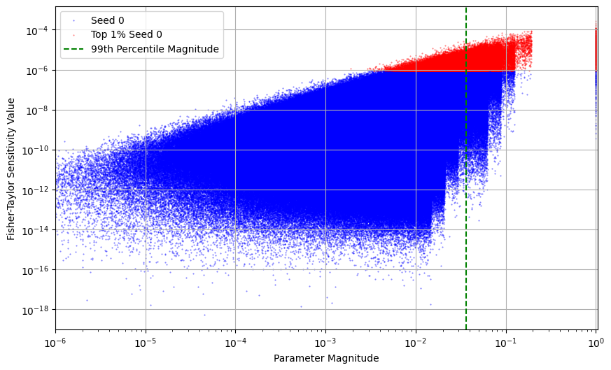
Figure 1: FTS vs. Magnitude parameter selection for 99% sparsity (ResNet18, CIFAR-10, Seed 0): We evaluated the relationship between the magnitude of the parameters and our best-performing criterion. The red area represents the parameters selected by our criterion. In contrast, the area to the right of the vertical line represents those that would have been selected if we chose the magnitude-based approach.

Table 2: Performance of different pruning methods evaluated on VGG19 with CIFAR-10 at extreme sparsity ratios. The table compares results with and without a 1-epoch warm-up. Bold values highlight the best-performing mean accuracy, while methods with comparable performance (within the best method’s standard deviation) are underlined.

Sparsity (%)	Random	Magnitude	GN	SNIP	GraSP	FD	FP	FTS	FBSS
No Warm-Up
0.98	80.04 ± 0.90	10.00 ± 0.00	10.00 ± 0.00	10.00 ± 0.00	10.00 ± 0.00	10.00 ± 0.00	10.00 ± 0.00	10.00 ± 0.00	10.00 ± 0.00
0.99	76.89 ± 0.26	10.00 ± 0.00	10.00 ± 0.00	10.00 ± 0.00	10.00 ± 0.00	10.00 ± 0.00	10.00 ± 0.00	10.00 ± 0.00	10.00 ± 0.00
1-Epoch Warm-Up
0.98	83.47 ± 0.20	85.70 ± 0.33	86.43 ± 0.05	87.26 ± 0.28	85.99 ± 0.08	85.61 ±0 .20	86.97 ± 0.22	87.24 ± 0.32	83.40 ± 0.74
0.99	78.28 ± 0.45	71.99 ± 0.28	83.47 ± 0.15	84.54 ± 0.04	84.56 ± 0.46	82.13 ± 0.28	83.74 ± 0.48	84.85 ± 0.18	77.60 ± 1.02

Preventing Layer Collapse. Table A3 (Appendix D.2) summarizes the performance of different pruning criteria evaluated on the VGG19 architecture with the CIFAR-10 test set. For this architecture, all data-dependent pruning methods suffer a drastic performance drop at high and extreme sparsities, completely reducing the accuracy to $10.00\%$. This behavior is consistent with the layer collapse phenomenon described in Section 1, where pruning removes entire layers (or most of their parameters), severely disrupting the flow of information and rendering the network untrainable.

A simple yet effective solution to mitigate layer collapse is the introduction of a single warm-up epoch before pruning. This step stabilizes the gradients and ensures a more balanced pruning distribution across layers. Table 2 demonstrates the impact of this adjustment, illustrating that just minimal adjustment before pruning helps maintain information flow and prevents layer collapse, allowing successful learning in the pruned network. We observe similar trends on the CIFAR-100 dataset. In the appendix, refer to Section E.2.

Batch Size FIM Estimation. Figure 2 demonstrates the positive effect of utilizing a batched gradient-based estimation of the FIM diagonal for extreme sparsity ratios. We demonstrate that, especially at initialization, reducing the variance of our estimation utilizing large batch size $|B^{k}|$ is critical to effectively measure the sensitivity of parameters. Especially for the FBSS criterion, the batched FIM estimation might compensate for the limited diagonal representation. Given the successful performance regardless of the selected batch size, we highlight the robustness to noise of the proposed FTS criterion. We share details for other sparsity ratios in Appendix F.

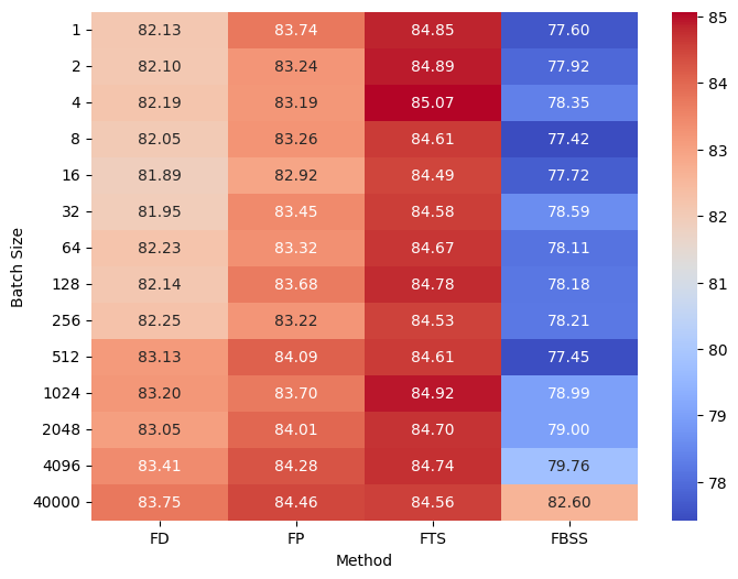
Figure 2: Effect of batch size of the mask in the final model accuracy for ResNet18 using CIFAR-10 dataset with 99% sparsity.

5 Conclusion

This work introduces FTS, a computationally cheap and efficient pruning criterion that leverages first- and second-order information to perform one-shot pruning at initialization. Our approach builds on the empirical FIM diagonal, demonstrating its effectiveness in finding important parameters, even with randomly initialized networks.

The experiments performed show that FTS consistently outperforms or matches the performance of state-of-the-art PBT methods, particularly at high and extreme sparsities. Furthermore, we demonstrated the positive effect of estimating the FIM diagonal with batched gradients to reduce the noise and computational overhead. In addition, we show that a single warm-up epoch mitigates layer collapse, allowing data-dependent pruning methods to maintain performance.

Our results highlight the practical advantages of FTS in identifying performant subnetworks at initialization, providing a scalable alternative to Hessian-based pruning. Our work contributes to advancing efficient deep learning and resource-aware model deployment. Future work includes refining the FIM approximation to capture off-diagonal interactions and extending our approach to larger architectures and real-world tasks.

Future research directions include exploring the integration of FTS with other compression techniques, such as quantization, for real-world applications. Exploring its synergy with modern training paradigms, including lottery ticket hypothesis-inspired approaches and adaptive sparsification, also presents promising avenues.

Impact Statement

This work aims to advance the field of Machine Learning by improving the efficiency of neural network pruning at initialization. By reducing the computational cost of training and inference while maintaining model performance, our approach lowers the hardware requirements for deploying AI systems. This contributes to the democratization of AI, making efficient deep learning models more accessible to researchers and practitioners with limited computational resources. While our work primarily focuses on technical advancements, it has broader implications for increasing the sustainability and inclusivity of AI development.

Appendix

Appendix A Optimal Brain Surgeon Derivation

In the original setup in OBS, we have a local quadratic model for the loss $L$ given by:

$$\delta L=L(w+\delta w)\approx L(w)+\nabla_{w}L^{T}\delta w+\frac{1}{2}\delta w^{T}H\delta w$$

Since OBS is a pruning-after-training approach, they discarded the 1-st order component. Reducing the expression for saliency as:

$$\delta L=\frac{1}{2}\delta w^{T}H\delta w$$

To remove a single parameter, the authors of OBS introduced the constraint $e_{q}^{T}\delta w+w_{q}=0$, with $e_{q}$ being the $q^{\text{th}}$ canonical basis vector. The pruning is defined as a constrained optimization problem of the form:

$$\min_{\delta w\in\mathbb{R^{d}}}\left(\frac{1}{2}\delta w^{T}H\delta w\right),~~\text{s.t}~~e_{q}^{T}\delta w+w_{q}=0.$$

And the choice of which parameter to remove becomes:

$$\min_{q\in\mathcal{Q}}\left\{\min_{\delta w\in\mathbb{R^{d}}}\left(\frac{1}{2}\delta w^{T}H\delta w\right),~~\text{s.t}~~e_{q}^{T}\delta w+w_{q}=0\right\}.$$

To solve the internal problem, we use a Lagrange multiplier $\lambda$ to write the problem as an unconstrained optimization case as follows:

$$\mathcal{L}(\delta w,\lambda)=\frac{1}{2}\delta w^{T}H\delta w+\lambda(e_{q}^{T}\delta w+w_{q}).$$

Then, to find the stationary conditions, we compute the partial derivatives with respect to $\delta w$ and $\lambda$, and equate them to 0, obtaining:

$$\nabla_{\delta w}\mathcal{L}=H\delta w+\lambda e_{q}=0\rightarrow\delta w=-\lambda H^{-1}e_{q}$$

$$\nabla_{\lambda}\mathcal{L}=e_{q}^{T}\delta w+w_{q}=0\rightarrow e_{q}^{T}\delta w=-w_{q}$$

With some replacements, we get:

$$e_{q}^{T}\delta w=-w_{q}\rightarrow e_{q}^{T}\left(-\lambda H^{-1}e_{q}\right)=-w_{q}\rightarrow-\lambda e_{q}^{T}H^{-1}e_{q}=-w_{q}\rightarrow\lambda=\frac{w_{q}}{e_{q}^{T}H^{-1}e_{q}}=\frac{w_{q}}{[H^{-1}]_{qq}}$$

$$\delta w=-\frac{w_{q}H^{-1}e_{q}}{[H^{-1}]_{qq}}$$

Replacing the expression for $\delta w$ in the saliency expression, we have:

$$\delta L=\frac{1}{2}\delta w^{T}H\delta w =\frac{1}{2}\left(-\frac{w_{q}H^{-1}e_{q}}{[H^{-1}]_{qq}}\right)^{T}H\left(-\frac{w_{q}H^{-1}e_{q}}{[H^{-1}]_{qq}}\right)$$

$$=\frac{w_{q}^{2}}{2[H^{-1}]_{qq}^{2}}\left(H^{-1}e_{q}\right)^{T}H\left(H^{-1}e_{q}\right)$$

$$=\frac{w_{q}^{2}}{2[H^{-1}]_{qq}^{2}}e_{q}^{T}H^{-1}e_{q}=\frac{w_{q}^{2}}{2[H^{-1}]_{qq}^{2}}[H^{-1}]_{qq}=\frac{w_{q}^{2}}{2[H^{-1}]_{qq}}$$

Appendix B Fisher Brain Surgeon Sensitivity Derivation

As we considered a PBT setting, it is not possible to ignore the first-order term in the local quadratic approximation of the error as it could still be informative. In this case, our model for sensitivity is given by:

$$\delta L=\nabla_{w}L^{T}\delta w+\frac{1}{2}\delta w^{T}H\delta w$$

The process to remove a single parameter remains similar; the constraint $e_{q}^{T}\delta w+w_{q}=0$, with $e_{q}$ is still valid, redefining the optimization problem as:

$$\min_{\delta w\in\mathbb{R^{d}}}\left(\nabla_{w}L^{T}\delta w+\frac{1}{2}\delta w^{T}H\delta w\right),~~\text{s.t}~~e_{q}^{T}\delta w+w_{q}=0.$$

And the choice of which parameter to remove becomes:

$$\min_{q\in\mathcal{Q}}\left\{\min_{\delta w\in\mathbb{R^{d}}}\left(\nabla_{w}L^{T}\delta w+\frac{1}{2}\delta w^{T}H\delta w\right),~~\text{s.t}~~e_{q}^{T}\delta w+w_{q}=0\right\}.$$

Using a Lagrange multiplier $\lambda$ as in the reference case, we solve the following unconstrained optimization problem:

$$\mathcal{L}(\delta w,\lambda)=\nabla_{w}L^{T}\delta w+\frac{1}{2}\delta w^{T}H\delta w+\lambda(e_{q}^{T}\delta w+w_{q}).$$

With the following stationary conditions:

$$\nabla_{\delta w}\mathcal{L}=\nabla_{w}L+H\delta w+\lambda e_{q}=0\rightarrow\delta w=-(\lambda H^{-1}e_{q}+H^{-1}\nabla_{w}L)$$

$$\nabla_{\lambda}\mathcal{L}=e_{q}^{T}\delta w+w_{q}=0\rightarrow e_{q}^{T}\delta w=-w_{q}$$

The expression for $\lambda$ is redefined as follows:

$$e_{q}^{T}\left(-(\lambda H^{-1}e_{q}+H^{-1}\nabla_{w}L)\right) =-w_{q}$$

$$\lambda e_{q}^{T}H^{-1}e_{q}+e_{q}^{T}H^{-1}\nabla_{w}L =w_{q}$$

$$\lambda[H^{-1}]_{qq} =w_{q}-e_{q}^{T}H^{-1}\nabla_{w}L$$

$$\lambda =\frac{w_{q}-e_{q}^{T}H^{-1}\nabla_{w}L}{[H^{-1}]_{qq}}$$

Replacing the expression for $\delta w$ in our sensitivity expression, we have:

$$\delta L=\nabla_{w}L^{T}\delta w+\frac{1}{2}\delta w^{T}H\delta w =\nabla_{w}L^{T}\left[-(\lambda H^{-1}e_{q}+H^{-1}\nabla_{w}L)\right]$$

$$+\frac{1}{2}\left[-(\lambda H^{-1}e_{q}+H^{-1}\nabla_{w}L)\right]^{T}H\left[-(\lambda H^{-1}e_{q}+H^{-1}\nabla_{w}L)\right]$$

$$=-\lambda\nabla_{w}L^{T}H^{-1}e_{q}-\nabla_{w}L^{T}H^{-1}\nabla_{w}L$$

$$+\frac{1}{2}\left[(\lambda H^{-1}e_{q})^{T}+(H^{-1}\nabla_{w}L)^{T}\right]\left[\lambda HH^{-1}e_{q}+HH^{-1}\nabla_{w}L)\right]$$

$$=-\lambda\nabla_{w}L^{T}H^{-1}e_{q}-\nabla_{w}L^{T}H^{-1}\nabla_{w}L$$

$$+\frac{1}{2}\left[(\lambda H^{-1}e_{q})^{T}+(H^{-1}\nabla_{w}L)^{T}\right]\left[\lambda e_{q}+\nabla_{w}L\right]$$

$$=-\lambda\nabla_{w}L^{T}H^{-1}e_{q}-\nabla_{w}L^{T}H^{-1}\nabla_{w}L$$

$$+\frac{1}{2}\left[(\lambda H^{-1}e_{q})^{T}\lambda e_{q}+(H^{-1}\nabla_{w}L)^{T}\lambda e_{q}+(\lambda H^{-1}e_{q})^{T}\nabla_{w}L+(H^{-1}\nabla_{w}L)^{T}\nabla_{w}L\right]$$

$$=-\lambda\nabla_{w}L^{T}H^{-1}e_{q}-\nabla_{w}L^{T}H^{-1}\nabla_{w}L$$

$$+\frac{1}{2}\left[\lambda^{2}e_{q}^{T}H^{-1}e_{q}+\lambda\nabla_{w}L^{T}H^{-1}e_{q}+\lambda e_{q}^{T}H^{-1}\nabla_{w}L+\nabla_{w}L^{T}H^{-1}\nabla_{w}L\right]$$

$$=\frac{1}{2}\left[\lambda^{2}[H^{-1}]_{qq}-\lambda\nabla_{w}L^{T}H^{-1}e_{q}+\lambda e_{q}^{T}H^{-1}\nabla_{w}L-\nabla_{w}L^{T}H^{-1}\nabla_{w}L\right]$$

Finally, replacing the $\lambda$:

$$\delta L =\frac{1}{2}\left[\lambda^{2}[H^{-1}]_{qq}-\lambda\nabla_{w}L^{T}H^{-1}e_{q}+\lambda e_{q}^{T}H^{-1}\nabla_{w}L-\nabla_{w}L^{T}H^{-1}\nabla_{w}L\right]$$

$$=\frac{1}{2[H^{-1}]_{qq}}\left[(w_{q}-e_{q}^{T}H^{-1}\nabla_{w}L)^{2}+(w_{q}-e_{q}^{T}H^{-1}\nabla_{w}L)(e_{q}^{T}H^{-1}\nabla_{w}L-\nabla_{w}L^{T}H^{-1}e_{q})-\nabla_{w}L^{T}H^{-1}\nabla_{w}L\right]$$

$$=\frac{1}{2[H^{-1}]_{qq}}[w_{q}^{2}-2w_{q}(e_{q}^{T}H^{-1}\nabla_{w}L)+(e_{q}^{T}H^{-1}\nabla_{w}L)^{2}+w_{q}(e_{q}^{T}H^{-1}\nabla_{w}L)$$

$$-w_{q}(\nabla_{w}L^{T}H^{-1}e_{q})-(e_{q}^{T}H^{-1}\nabla_{w}L)(e_{q}^{T}H^{-1}\nabla_{w}L)+(e_{q}^{T}H^{-1}\nabla_{w}L)(\nabla_{w}L^{T}H^{-1}e_{q})-\nabla_{w}L^{T}H^{-1}\nabla_{w}L]$$

$$=\frac{1}{2[H^{-1}]_{qq}}[w_{q}^{2}-w_{q}(e_{q}^{T}H^{-1}\nabla_{w}L)+(e_{q}^{T}H^{-1}\nabla_{w}L)^{2}$$

$$-w_{q}(\nabla_{w}L^{T}H^{-1}e_{q})-(e_{q}^{T}H^{-1}\nabla_{w}L)^{2}+(e_{q}^{T}H^{-1}\nabla_{w}L)(\nabla_{w}L^{T}H^{-1}e_{q})-\nabla_{w}L^{T}H^{-1}\nabla_{w}L]$$

$$=\frac{1}{2[H^{-1}]_{qq}}\left[w_{q}^{2}-2w_{q}(e_{q}^{T}H^{-1}\nabla_{w}L)+(e_{q}^{T}H^{-1}\nabla_{w}L)^{2}-\nabla_{w}L^{T}H^{-1}\nabla_{w}L\right]$$

$$=\frac{1}{2[\hat{F}^{-1}]_{qq}}\left[w_{q}-(e_{q}^{T}\hat{F}^{-1}\nabla\mathcal{L}(w_{0}))\right]^{2}$$

Appendix C Training and Testing Details

We perform an 80:20 stratified split, with a constant seed, on the CIFAR10/100 training dataset to obtain a validation set with the same class distribution. For both datasets, we have a training set with 40,000 samples, a validation set with 10,000 samples, and a testing set of 10,000 samples. Validation is performed after each training step, and the weights of the best-performing validation step (based on top-1 accuracy) are utilized for the final evaluation on the testing set. Table A1 summarizes the training parameters.

Table A1: Training parameters used for ResNet18 and VGG19 on the CIFAR-10/100 datasets.

Parameter	ResNet18	VGG19
Number of steps	160	160
Criterion	CE	CE
Optimizer	SGD	SGD
Learning rate	0.01	0.1
Momentum	0.9	0.9
Weight decay	$5\times 10^{-4}$	$1\times 10^{-4}$
Learning rate drops	[60, 120]	[60, 120]
Learning rate drop factor	0.2	0.1

Appendix D Results CIFAR10

D.1 ResNet18

Table A2: Performance of different sensitivity methods for pruning evaluated using ResNet18 on the CIFAR-10 testset. The right side of the table presents our proposed criteria. The mean accuracy and standard deviation are reported across three initialization seeds for various sparsity levels. Baseline, no pruning: $91.78\pm 0.09$.

Sparsity	Random	Magnitude	GN	SNIP	GraSP	FD	FP	FTS	FBSS
0.10	91.71 ± 0.21	91.72 ± 0.07	91.57 ± 0.15	91.72 ± 0.07	89.16 ± 0.05	91.87 ± 0.13	91.63 ± 0.21	91.53 ± 0.12	91.76 ± 0.08
0.20	91.63 ± 0.11	91.42 ± 0.12	91.51 ± 0.09	91.64 ± 0.16	88.69 ± 0.34	91.50 ± 0.12	91.65 ± 0.14	91.53 ± 0.15	91.54 ± 0.13
0.30	91.45 ± 0.18	91.61 ± 0.13	91.68 ± 0.20	91.65 ± 0.08	88.67 ± 0.26	91.65 ± 0.18	91.44 ± 0.27	91.49 ± 0.05	91.62 ± 0.07
0.40	91.59 ± 0.18	91.06 ± 0.16	91.61 ± 0.09	91.55 ± 0.08	88.24 ± 0.33	91.51 ± 0.05	91.38 ± 0.13	91.56 ± 0.28	91.39 ± 0.05
0.50	91.60 ± 0.06	91.32 ± 0.13	91.44 ± 0.13	91.22 ± 0.07	87.69 ± 0.15	91.30 ± 0.18	91.58 ± 0.16	91.46 ± 0.19	91.41 ± 0.05
0.60	91.10 ± 0.16	91.18 ± 0.16	91.59 ± 0.13	91.24 ± 0.04	87.48 ± 0.55	91.34 ± 0.07	91.35 ± 0.16	91.40 ± 0.11	91.38 ± 0.18
0.70	91.17 ± 0.04	91.07 ± 0.07	91.19 ± 0.17	91.33 ± 0.18	87.26 ± 0.34	91.34 ± 0.23	91.42 ± 0.23	91.18 ± 0.18	91.27 ± 0.14
0.80	90.78 ± 0.08	91.10 ± 0.12	90.95 ± 0.35	90.74 ± 0.10	87.18 ± 0.51	90.95 ± 0.11	91.08 ± 0.06	90.94 ± 0.22	90.73 ± 0.33
0.90	89.35 ± 0.13	89.88 ± 0.28	90.39 ± 0.23	90.36 ± 0.34	86.60 ± 0.51	90.04 ± 0.21	90.20 ± 0.08	90.55 ± 0.23	89.22 ± 0.30
0.95	87.59 ± 0.11	89.23 ± 0.19	89.00 ± 0.05	89.31 ± 0.17	86.50 ± 0.05	88.61 ± 0.28	89.50 ± 0.18	89.47 ± 0.32	87.58 ± 0.25
0.98	83.47 ± 0.20	85.70 ± 0.33	86.43 ± 0.05	87.26 ± 0.28	85.99 ± 0.08	85.61 ± 0.20	86.97 ± 0.22	87.24 ± 0.32	83.40 ± 0.74
0.99	78.28 ± 0.45	71.99 ± 0.28	83.47 ± 0.15	84.54 ± 0.04	84.56 ± 0.46	82.13 ± 0.28	83.74 ± 0.48	84.85 ± 0.18	77.60 ± 1.02

D.2 VGG19

As discussed earlier, introducing a warm-up phase effectively mitigates layer collapse in data-dependent pruning methods. Here, we evaluate the impact of different warm-up durations by comparing no warm-up, a single warm-up epoch, and five warm-up epochs. Table A3 demonstrates how performance drastically degrades with increasing sparsity, ultimately leading to layer collapse at 0.90 sparsity. However, as shown in the results, a single warm-up epoch is sufficient to prevent collapse and stabilize pruning performance. Moreover, as seen in Table A5, increasing the warm-up period to five epochs provides no substantial additional improvement. This indicates that prolonged warm-up training is not necessary; a single training step is enough to achieve gradient stabilization and overcome layer collapse.

Table A3: Performance of different sensitivity methods for pruning evaluated using VGG19 on the CIFAR-10 test set. The right side of the table presents our proposed criteria. The mean accuracy and standard deviation are reported across three initialization seeds for various sparsity levels. Baseline, no pruning: $89.21\pm 0.22$.

Sparsity	Random	Magnitude	GN	SNIP	GraSP	FD	FP	FTS	FBSS
0.10	88.40 ± 0.95	89.12 ± 0.55	90.14 ± 0.10	90.16 ± 0.18	87.81 ± 1.66	90.20 ± 0.29	90.21 ± 0.37	90.25 ± 0.38	89.06 ± 0.75
0.20	89.19 ± 0.22	89.65 ± 0.60	89.59 ± 0.69	90.06 ± 0.04	89.57 ± 0.34	89.91 ± 0.28	90.28 ± 0.55	89.80 ± 0.28	88.89 ± 0.76
0.30	88.93 ± 0.83	88.77 ± 1.07	90.23 ± 0.09	89.88 ± 0.59	89.14 ± 0.19	90.25 ± 0.09	89.97 ± 0.26	90.46 ± 0.41	89.06 ± 0.36
0.40	88.28 ± 1.08	89.38 ± 0.53	90.50 ± 0.23	89.79 ± 0.67	88.20 ± 0.31	90.51 ± 0.12	90.37 ± 0.24	90.23 ± 0.14	10.00 ± 0.00
0.50	88.96 ± 0.82	89.03 ± 0.59	90.46 ± 0.60	90.38 ± 0.25	88.67 ± 0.23	89.54 ± 0.86	90.47 ± 0.52	90.19 ± 0.31	10.00 ± 0.00
0.60	88.15 ± 0.68	89.47 ± 0.18	89.95 ± 0.30	90.32 ± 0.25	88.82 ± 0.32	90.02 ± 0.40	90.18 ± 0.33	90.14 ± 0.36	10.00 ± 0.00
0.70	88.02 ± 0.53	89.63 ± 0.44	89.69 ± 0.42	89.23 ± 0.19	89.62 ± 0.81	89.85 ± 0.08	90.01 ± 0.34	10.00 ± 0.00	10.00 ± 0.00
0.80	88.28 ± 0.34	89.62 ± 0.91	85.72 ± 0.63	89.39 ± 0.43	88.82 ± 0.14	10.00 ± 0.00	88.29 ± 0.11	10.00 ± 0.00	10.00 ± 0.00
0.90	85.82 ± 0.19	89.29 ± 0.79	10.00 ± 0.00	80.85 ± 0.62	24.28 ± 20.2	10.00 ± 0.00	10.00 ± 0.00	10.00 ± 0.00	10.00 ± 0.00
0.95	84.41 ± 0.05	10.00 ± 0.00	10.00 ± 0.00	10.00 ± 0.00	10.00 ± 0.00	10.00 ± 0.00	10.00 ± 0.00	10.00 ± 0.00	10.00 ± 0.00
0.98	80.04 ± 0.90	10.00 ± 0.00	10.00 ± 0.00	10.00 ± 0.00	10.00 ± 0.00	10.00 ± 0.00	10.00 ± 0.00	10.00 ± 0.00	10.00 ± 0.00
0.99	76.89 ± 0.26	10.00 ± 0.00	10.00 ± 0.00	10.00 ± 0.00	10.00 ± 0.00	10.00 ± 0.00	10.00 ± 0.00	10.00 ± 0.00	10.00 ± 0.00

Table A4: Performance of different compression methods evaluated after 1 warmup epoch using VGG19 on the CIFAR-10 dataset. We report the mean accuracy between three initialization seeds across various sparsity levels. Baseline, no pruning: $89.21\pm 0.22$.

Sparsity	Random	Magnitude	GN	SNIP	GraSP	FD	FP	FTS	FBSS
0.80	88.73 ± 0.38	88.35 ± 0.54	86.76 ± 0.27	87.39 ± 0.66	87.24 ± 0.25	87.14 ± 0.45	87.00 ± 0.87	87.68 ± 0.33	64.33 ± 15.91
0.90	87.26 ± 0.42	88.62 ± 0.49	85.96 ± 0.75	86.75 ± 0.76	87.47 ± 0.33	86.69 ± 0.72	87.09 ± 0.31	87.42 ± 0.21	46.16 ± 7.62
0.95	85.47 ± 0.64	87.68 ± 0.49	86.66 ± 0.27	86.00 ± 1.10	86.71 ± 1.24	85.71 ± 1.35	86.73 ± 0.36	87.56 ± 0.62	46.30 ± 5.32
0.98	80.44 ± 0.30	86.61 ± 0.62	84.72 ± 1.69	87.22 ± 0.23	86.45 ± 0.64	80.34 ± 6.43	86.07 ± 0.39	86.36 ± 0.29	49.05 ± 4.31
0.99	77.24 ± 0.73	83.69 ± 1.36	80.28 ± 2.04	83.49 ± 1.77	85.39 ± 0.43	75.11 ± 7.80	84.40 ± 1.27	85.35 ± 1.05	47.10 ± 4.41

Table A5: Performance of different sensitivity methods for pruning evaluated after 5 warmup epochs using VGG19 on the CIFAR-10 testset. The right side of the table presents our proposed criteria. The mean accuracy and standard deviation are reported across three initialization seeds for various sparsity levels. Baseline, no pruning: $89.21\pm 0.22$.

Sparsity	Random	Magnitude	GN	SNIP	GraSP	FD	FP	FTS	FBSS
0.80	88.84 ± 0.43	88.41 ± 0.47	87.58 ± 0.52	88.15 ± 1.09	86.77 ± 1.14	87.28 ± 0.90	88.22 ± 0.82	86.68 ± 0.61	70.52 ± 9.25
0.90	87.56 ± 0.62	88.60 ± 0.93	86.73 ± 0.37	87.89 ± 0.25	87.10 ± 0.47	87.50 ± 1.42	88.18 ± 0.47	86.98 ± 0.14	47.78 ± 1.26
0.95	85.51 ± 0.69	87.66 ± 1.19	87.44 ± 0.46	87.71 ± 0.82	87.05 ± 0.16	86.83 ± 1.47	87.36 ± 0.52	87.00 ± 0.74	48.83 ± 2.52
0.98	82.09 ± 0.17	86.24 ± 0.52	84.66 ± 1.33	86.55 ± 0.84	86.04 ± 0.66	85.44 ± 0.64	86.64 ± 0.13	84.89 ± 0.51	49.48 ± 0.85
0.99	77.22 ± 1.03	83.93 ± 1.80	81.62 ± 2.17	84.53 ± 0.70	81.33 ± 5.77	81.71 ± 1.41	85.02 ± 0.69	83.78 ± 0.80	41.24 ± 1.55

Appendix E Results CIFAR100

E.1 ResNet18

CIFAR-100 results exhibit a similar trend to those observed on CIFAR-10, further reinforcing the robustness of our proposed Fisher-Taylor Sensitivity (FTS) criterion. Across all evaluated sparsity levels, FTS consistently maintains strong performance, frequently ranking among the top-performing methods. This trend is particularly evident at extreme sparsities, where many pruning approaches suffer significant performance degradation. The stability of FTS across both datasets highlights its effectiveness in preserving network expressivity despite aggressive pruning.

Table A6: Performance of different compression methods evaluated using ResNet18 on the CIFAR-100 dataset. We report the mean accuracy between three initialization seeds across various sparsity levels. Baseline, no pruning: $69.57\pm 0.19$.

Sparsity	Random	Magnitude	GN	SNIP	GraSP	FD	FP	FTS	FBSS
0.10	69.16 ± 0.11	69.37 ± 0.14	69.63 ± 0.34	69.42 ± 0.07	64.26 ± 0.27	69.66 ± 0.30	69.08 ± 0.21	69.16 ± 0.11	69.07 ± 0.10
0.20	69.16 ± 0.30	69.06 ± 0.24	69.19 ± 0.11	69.30 ± 0.08	63.28 ± 0.58	69.60 ± 0.30	69.35 ± 0.35	69.41 ± 0.43	69.07 ± 0.20
0.30	69.36 ± 0.18	68.58 ± 0.36	69.37 ± 0.13	68.82 ± 0.17	62.02 ± 0.43	69.24 ± 0.40	68.84 ± 0.13	68.80 ± 0.55	68.96 ± 0.11
0.40	69.41 ± 0.20	68.50 ± 0.29	69.16 ± 0.26	68.95 ± 0.19	61.18 ± 0.19	69.17 ± 0.16	68.88 ± 0.25	69.02 ± 0.21	68.92 ± 0.25
0.50	69.12 ± 0.46	68.17 ± 0.20	68.94 ± 0.20	68.63 ± 0.11	61.11 ± 0.40	69.13 ± 0.13	68.68 ± 0.12	68.71 ± 0.12	68.71 ± 0.57
0.60	68.66 ± 0.27	67.78 ± 0.35	68.77 ± 0.17	68.63 ± 0.42	61.40 ± 0.78	68.34 ± 0.43	67.98 ± 0.23	68.41 ± 0.14	68.60 ± 0.15
0.70	67.95 ± 0.43	67.51 ± 0.24	68.29 ± 0.39	68.08 ± 0.18	59.43 ± 0.76	68.03 ± 0.46	67.96 ± 0.15	68.29 ± 0.06	68.16 ± 0.07
0.80	67.26 ± 0.48	66.55 ± 0.19	67.20 ± 0.37	67.21 ± 0.38	59.08 ± 0.22	66.70 ± 0.05	67.05 ± 0.06	66.77 ± 0.65	66.62 ± 0.43
0.90	64.75 ± 0.16	64.48 ± 0.18	64.87 ± 0.27	65.70 ± 0.08	59.16 ± 0.91	64.74 ± 0.44	65.46 ± 0.30	65.41 ± 0.13	63.90 ± 0.31
0.95	61.01 ± 0.32	62.20 ± 0.06	62.20 ± 0.23	63.20 ± 0.20	57.91 ± 0.09	62.14 ± 0.42	63.22 ± 0.25	63.21 ± 0.47	61.25 ± 0.44
0.98	54.72 ± 0.22	55.44 ± 0.18	57.34 ± 0.31	58.83 ± 0.35	54.85 ± 0.35	55.57 ± 0.17	58.05 ± 0.18	58.59 ± 0.12	55.02 ± 0.34
0.99	45.62 ± 0.55	40.39 ± 0.36	50.46 ± 0.61	52.96 ± 0.10	49.13 ± 0.19	48.02 ± 0.32	49.98 ± 0.60	52.85 ± 0.24	44.91 ± 0.52

E.2 VGG19

The results on VGG19 with CIFAR-100 exhibit a similar trend to those observed on CIFAR-10, reinforcing the effectiveness of our proposed approach. Once again, we identify the occurrence of layer collapse at extreme sparsities when no warm-up is applied, leading to a significant drop in accuracy. Introducing a single warm-up epoch effectively resolves this issue, restoring pruning performance across all evaluated criteria. However, increasing the warm-up phase to five epochs does not yield any additional advantage, indicating that a brief warm-up period is sufficient to stabilize gradient-based importance scores and prevent collapse.

Table A7: Performance of different compression methods evaluated using VGG19 on the CIFAR-100 dataset. We report the mean accuracy between three initialization seeds across various sparsity levels. Baseline, no pruning: $58.96\pm 2.30$.

Sparsity	Random	Magnitude	GN	SNIP	GraSP	FD	FP	FTS	FBSS
0.10	60.31 ± 0.40	59.13 ± 1.29	61.93 ± 0.48	61.98 ± 0.29	59.32 ± 0.63	62.13 ± 0.61	60.45 ± 3.47	61.56 ± 1.04	58.79 ± 0.98
0.20	60.43 ± 1.14	59.27 ± 0.34	62.64 ± 0.21	62.68 ± 0.24	61.21 ± 0.41	63.04 ± 0.43	62.71 ± 1.02	62.24 ± 0.44	60.48 ± 0.48
0.30	58.32 ± 0.60	59.35 ± 1.43	62.61 ± 0.23	63.11 ± 0.35	59.30 ± 0.43	62.85 ± 0.42	61.43 ± 0.61	62.65 ± 0.54	58.77 ± 1.02
0.40	56.50 ± 3.20	60.04 ± 1.02	62.36 ± 0.02	62.39 ± 0.55	56.34 ± 1.49	62.38 ± 0.75	61.56 ± 1.25	62.67 ± 0.06	1.00 ± 0.00
0.50	58.47 ± 1.49	61.49 ± 1.22	62.02 ± 0.64	62.76 ± 0.50	54.43 ± 0.84	62.84 ± 0.33	62.25 ± 0.33	62.47 ± 0.42	1.00 ± 0.00
0.60	57.54 ± 0.74	61.50 ± 0.30	62.55 ± 0.13	63.08 ± 0.55	56.76 ± 0.69	62.40 ± 0.57	62.70 ± 0.63	62.17 ± 0.23	1.00 ± 0.00
0.70	57.63 ± 0.80	61.71 ± 0.25	60.85 ± 0.79	60.58 ± 0.39	57.76 ± 0.84	60.44 ± 0.34	60.92 ± 0.41	60.51 ± 1.67	1.00 ± 0.00
0.80	57.84 ± 0.57	61.89 ± 1.02	55.09 ± 0.49	59.84 ± 0.29	58.39 ± 0.74	1.00 ± 0.00	43.16 ± 1.02	58.66 ± 2.28	1.00 ± 0.00
0.90	58.41 ± 0.41	62.60 ± 0.91	1.00 ± 0.00	8.35 ± 10.39	42.88 ± 1.64	1.00 ± 0.00	1.00 ± 0.00	8.87 ± 11.13	1.00 ± 0.00
0.95	54.84 ± 1.08	1.00 ± 0.00	1.00 ± 0.00	1.00 ± 0.00	1.00 ± 0.00	1.00 ± 0.00	1.00 ± 0.00	1.00 ± 0.00	1.00 ± 0.00
0.98	50.21 ± 0.72	1.00 ± 0.00	1.00 ± 0.00	1.00 ± 0.00	1.00 ± 0.00	1.00 ± 0.00	1.00 ± 0.00	1.00 ± 0.00	1.00 ± 0.00
0.99	46.69 ± 0.45	1.00 ± 0.00	1.00 ± 0.00	1.00 ± 0.00	1.00 ± 0.00	1.00 ± 0.00	1.00 ± 0.00	1.00 ± 0.00	1.00 ± 0.00

Table A8: Performance of different compression methods evaluated after 1 warmup epoch using VGG19 on the CIFAR-100 dataset. We report the mean accuracy between three initialization seeds across various sparsity levels. Baseline, no pruning: $58.96\pm 2.30$.

Sparsity	Random	Magnitude	GN	SNIP	GraSP	FD	FP	FTS	FBSS
0.80	60.39 ± 1.16	58.91 ± 0.41	52.81 ± 1.32	55.62 ± 2.27	55.15 ± 2.25	56.71 ± 0.31	58.03 ± 0.93	52.41 ± 3.07	52.74 ± 5.16
0.90	58.90 ± 0.98	60.95 ± 0.81	50.56 ± 4.59	55.89 ± 2.05	56.01 ± 1.58	52.07 ± 3.24	53.65 ± 0.57	52.45 ± 3.75	19.65 ± 1.68
0.95	56.10 ± 0.85	57.64 ± 2.63	50.34 ± 1.00	53.70 ± 3.60	56.16 ± 0.41	54.44 ± 1.38	53.24 ± 3.54	53.56 ± 1.26	17.24 ± 0.44
0.98	50.97 ± 0.40	54.66 ± 2.56	43.43 ± 5.32	50.19 ± 1.59	54.64 ± 1.50	42.75 ± 1.91	50.59 ± 3.39	48.56 ± 5.25	16.42 ± 0.64
0.99	46.52 ± 0.45	43.33 ± 5.83	33.90 ± 5.35	42.65 ± 5.32	45.98 ± 4.48	29.67 ± 8.49	49.11 ± 3.46	48.70 ± 2.59	13.25 ± 0.84

Table A9: Performance of different compression methods evaluated after 5 warmup epochs using VGG19 on the CIFAR-100 dataset. We report the mean accuracy between three initialization seeds across various sparsity levels. Baseline, no pruning: $58.96\pm 2.30$.

Sparsity	Random	Magnitude	GN	SNIP	GraSP	FD	FP	FTS	FBSS
0.80	60.41 ± 1.39	58.38 ± 0.85	60.86 ± 0.79	61.63 ± 0.45	56.25 ± 0.49	59.59 ± 0.76	59.37 ± 3.50	60.86 ± 0.53	46.93 ± 9.04
0.90	60.32 ± 0.09	57.74 ± 1.64	57.77 ± 2.41	58.23 ± 4.07	56.27 ± 1.02	60.19 ± 0.63	61.23 ± 0.50	60.52 ± 0.37	21.66 ± 1.95
0.95	57.86 ± 0.53	59.55 ± 1.15	56.09 ± 0.97	58.83 ± 0.65	55.26 ± 1.25	55.80 ± 2.77	59.83 ± 0.94	58.52 ± 1.32	19.98 ± 2.62
0.98	51.75 ± 0.43	47.75 ± 7.63	52.26 ± 4.06	55.27 ± 1.69	54.59 ± 0.96	49.46 ± 4.98	57.40 ± 1.26	56.00 ± 1.08	17.59 ± 1.36
0.99	47.59 ± 0.80	42.46 ± 7.95	46.58 ± 2.00	53.13 ± 0.84	53.91 ± 1.53	42.87 ± 4.63	53.17 ± 1.18	53.05 ± 2.14	13.92 ± 0.14

Appendix F Mask Batch Size for Other Sparsities

The Effect of batch size on pruning performance across different sparsities. As sparsity increases, the effect of batch size on pruning performance becomes more pronounced. At lower sparsities (0.90, 0.95), the differences across batch sizes are less evident, suggesting that even smaller batches provide a reasonable estimation of parameter importance. However, at extreme sparsities (0.98, 0.99), we observe a clear trend where larger batch sizes consistently lead to better parameter selection, ultimately improving accuracy. This aligns with our hypothesis that larger batches help reduce variance in gradient estimation, leading to more stable and effective pruning decisions.

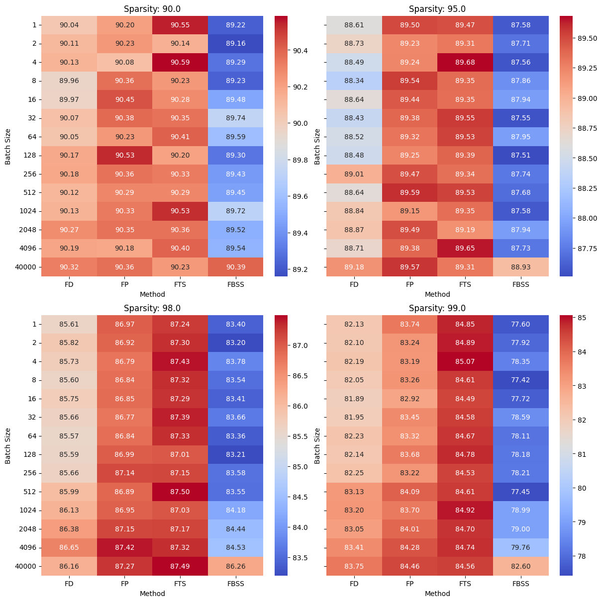
Figure A1: Effect of batch size on pruning performance at increasing sparsities.

Appendix G Comparison of our criteria with magnitude-based pruning

Figure A2 illustrates the relationship between parameter magnitude and different sensitivity-based pruning metrics. Each point represents a model parameter, with red points indicating the top-ranked parameters selected for retention by each criterion. The green dashed line marks the 99th percentile of parameter magnitudes.

A key observation is that the most effective pruning criteria, such as Fisher-Taylor Sensitivity, tend to retain parameters with a broad range of magnitudes, including many that are relatively small (left of the green line). This shows that the estimated importance does not always prioritize parameters based on their magnitude.

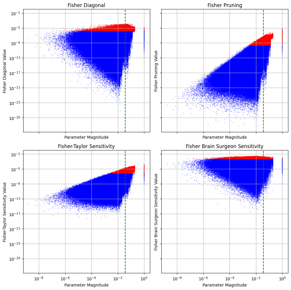
Figure A2: Our criteria vs. Magnitude parameter selection for 99% sparsity (ResNet18, CIFAR-10, Seed 0)

References

- Cheng et al. (2024) Cheng, H., Zhang, M., and Shi, J. Q. A survey on deep neural network pruning: Taxonomy, comparison, analysis, and recommendations. IEEE Transactions on Pattern Analysis and Machine Intelligence, 2024.
- Chien et al. (2023) Chien, A. A., Lin, L., Nguyen, H., Rao, V., Sharma, T., and Wijayawardana, R. Reducing the carbon impact of generative ai inference (today and in 2035). In Proceedings of the 2nd workshop on sustainable computer systems, pp. 1–7, 2023.
- Denton et al. (2014) Denton, E. L., Zaremba, W., Bruna, J., LeCun, Y., and Fergus, R. Exploiting linear structure within convolutional networks for efficient evaluation. Advances in neural information processing systems, 27, 2014.
- Dettmers et al. (2023) Dettmers, T., Pagnoni, A., Holtzman, A., and Zettlemoyer, L. Qlora: efficient finetuning of quantized llms (2023). arXiv preprint arXiv:2305.14314, 52:3982–3992, 2023.
- Frankle & Carbin (2018) Frankle, J. and Carbin, M. The lottery ticket hypothesis: Finding sparse, trainable neural networks. arXiv preprint arXiv:1803.03635, 2018.
- Habehh & Gohel (2021) Habehh, H. and Gohel, S. Machine learning in healthcare. Current genomics, 22(4):291, 2021.
- Han et al. (2015) Han, S., Pool, J., Tran, J., and Dally, W. Learning both weights and connections for efficient neural network. Advances in neural information processing systems, 28, 2015.
- Hassibi & Stork (1992) Hassibi, B. and Stork, D. Second order derivatives for network pruning: Optimal brain surgeon. Advances in neural information processing systems, 5, 1992.
- He et al. (2016) He, K., Zhang, X., Ren, S., and Sun, J. Deep residual learning for image recognition. In Proceedings of the IEEE conference on computer vision and pattern recognition, pp. 770–778, 2016.
- Jacot et al. (2018) Jacot, A., Gabriel, F., and Hongler, C. Neural tangent kernel: Convergence and generalization in neural networks. Advances in neural information processing systems, 31, 2018.
- Karakida et al. (2019) Karakida, R., Akaho, S., and Amari, S.-i. Universal statistics of fisher information in deep neural networks: Mean field approach. In The 22nd International Conference on Artificial Intelligence and Statistics, pp. 1032–1041. PMLR, 2019.
- Khan & Al-Habsi (2020) Khan, A. I. and Al-Habsi, S. Machine learning in computer vision. Procedia Computer Science, 167:1444–1451, 2020.
- Krizhevsky et al. (2009) Krizhevsky, A., Hinton, G., et al. Learning multiple layers of features from tiny images. 2009.
- Kumar et al. (2024) Kumar, T., Luo, K., and Sellke, M. No free prune: Information-theoretic barriers to pruning at initialization. arXiv preprint arXiv:2402.01089, 2024.
- LeCun et al. (1989) LeCun, Y., Denker, J., and Solla, S. Optimal brain damage. Advances in neural information processing systems, 2, 1989.
- Lee et al. (2018) Lee, N., Ajanthan, T., and Torr, P. H. Snip: Single-shot network pruning based on connection sensitivity. arXiv preprint arXiv:1810.02340, 2018.
- Liu et al. (2021) Liu, L., Zhang, S., Kuang, Z., Zhou, A., Xue, J.-H., Wang, X., Chen, Y., Yang, W., Liao, Q., and Zhang, W. Group fisher pruning for practical network compression. In International Conference on Machine Learning, pp. 7021–7032. PMLR, 2021.
- Schervish (2012) Schervish, M. J. Theory of statistics. Springer series in statistics. Springer, New York, NY, 1995 edition, December 2012.
- Simonyan (2014) Simonyan, K. Very deep convolutional networks for large-scale image recognition. arXiv preprint arXiv:1409.1556, 2014.
- Singh & Alistarh (2020) Singh, S. P. and Alistarh, D. Woodfisher: Efficient second-order approximation for neural network compression. Advances in Neural Information Processing Systems, 33:18098–18109, 2020.
- Soen & Sun (2024) Soen, A. and Sun, K. Tradeoffs of diagonal fisher information matrix estimators. arXiv preprint arXiv:2402.05379, 2024.
- Soori et al. (2023) Soori, M., Arezoo, B., and Dastres, R. Artificial intelligence, machine learning and deep learning in advanced robotics, a review. Cognitive Robotics, 3:54–70, 2023.
- Sreenivasan et al. (2022) Sreenivasan, K., Sohn, J.-y., Yang, L., Grinde, M., Nagle, A., Wang, H., Xing, E., Lee, K., and Papailiopoulos, D. Rare gems: Finding lottery tickets at initialization. Advances in neural information processing systems, 35:14529–14540, 2022.
- Tanaka et al. (2020) Tanaka, H., Kunin, D., Yamins, D. L., and Ganguli, S. Pruning neural networks without any data by iteratively conserving synaptic flow. Advances in neural information processing systems, 33:6377–6389, 2020.
- Theis et al. (2018) Theis, L., Korshunova, I., Tejani, A., and Huszár, F. Faster gaze prediction with dense networks and fisher pruning. arXiv preprint arXiv:1801.05787, 2018.
- Torfi et al. (2020) Torfi, A., Shirvani, R. A., Keneshloo, Y., Tavaf, N., and Fox, E. A. Natural language processing advancements by deep learning: A survey. arXiv preprint arXiv:2003.01200, 2020.
- Vacar et al. (2011) Vacar, C., Giovannelli, J.-F., and Berthoumieu, Y. Langevin and hessian with fisher approximation stochastic sampling for parameter estimation of structured covariance. In 2011 IEEE International Conference on Acoustics, Speech and Signal Processing (ICASSP), pp. 3964–3967. IEEE, 2011.
- Wang et al. (2020) Wang, C., Zhang, G., and Grosse, R. Picking winning tickets before training by preserving gradient flow. arXiv preprint arXiv:2002.07376, 2020.
- Wu et al. (2022) Wu, C.-J., Raghavendra, R., Gupta, U., Acun, B., Ardalani, N., Maeng, K., Chang, G., Aga, F., Huang, J., Bai, C., et al. Sustainable ai: Environmental implications, challenges and opportunities. Proceedings of Machine Learning and Systems, 4:795–813, 2022.
- Xu et al. (2024) Xu, X., Li, M., Tao, C., Shen, T., Cheng, R., Li, J., Xu, C., Tao, D., and Zhou, T. A survey on knowledge distillation of large language models. arXiv preprint arXiv:2402.13116, 2024.
- You et al. (2022) You, H., Li, B., Sun, Z., Ouyang, X., and Lin, Y. Supertickets: Drawing task-agnostic lottery tickets from supernets via jointly architecture searching and parameter pruning. In European Conference on Computer Vision, pp. 674–690. Springer, 2022.
- Yvinec et al. (2022) Yvinec, E., Dapogny, A., Cord, M., and Bailly, K. Singe: Sparsity via integrated gradients estimation of neuron relevance. Advances in Neural Information Processing Systems, 35:35392–35403, 2022.
- Zhang et al. (2021) Zhang, M., Su, S. W., Pan, S., Chang, X., Abbasnejad, E. M., and Haffari, R. idarts: Differentiable architecture search with stochastic implicit gradients. In International Conference on Machine Learning, pp. 12557–12566. PMLR, 2021.