Constraining the Hubble Constant with a Simulated Full Covariance Matrix Using Neural Networks

Abstract

The Hubble parameter, $H(z)$, plays a crucial role in understanding the expansion history of the universe and constraining the Hubble constant, $\mathrm{H}_{0}$. The Cosmic Chronometers (CC) method provides an independent approach to measuring $H(z)$, but existing studies either neglect off-diagonal elements in the covariance matrix or use an incomplete covariance matrix, limiting the accuracy of $\mathrm{H}_{0}$ constraints. To address this, we use a Fully Connected Neural Network (FCNN) to simulate the full $33\times 33$ covariance matrix based on a previously proposed $15\times 15$ covariance matrix. We find that two key hyperparameters, epochs and batch size, significantly affect the simulation and introduce two criteria for selecting optimal values. Using the simulated covariance matrix, we constrain $\mathrm{H}_{0}$ via two independent methods: EMCEE and Gaussian Process. Our results show that different hyperparameter selection criteria lead to variations in the chosen combinations but have little impact on the final constrained $\mathrm{H}_{0}$. However, different epochs and batch size settings do affect the results. Incorporating the simulated covariance matrix increases the uncertainty in $\mathrm{H}_{0}$ compared to using no covariance matrix or only the proposed $15\times 15$ covariance matrix. The comparison between EMCEE and GP suggests that the constraint method itself also influences the final $\mathrm{H}_{0}$. These findings highlight the importance of properly modeling covariance in CC-based $\mathrm{H}_{0}$ constraints.

1 Introduction

The study of the universe’s evolution is a fundamental and highly significant astronomy research area. The Hubble parameter, $H(z)$, describes the expansion rate of the universe at a given redshift $z$, where a higher $z$ corresponds to an earlier epoch in the universe’s history. Accurate measurements of $H(z)$ are crucial for understanding the dynamics of cosmic expansion and the nature of dark energy. Various methods have been developed to measure $H(z)$, including Type Ia Supernovae (SNe Ia) (Riess et al., 1998; Perlmutter et al., 1999), Baryon Acoustic Oscillations (Eisenstein et al., 2005; Alam et al., 2017), and Cosmic Chronometers (CC) (Jimenez & Loeb, 2002), among others. The $H(z)$ dataset can be used to constrain the Hubble constant, $\mathrm{H}_{0}$, which represents the present-day expansion rate of the universe. Two key approaches to measuring $\mathrm{H}_{0}$, the analysis of cosmic microwave background (CMB) anisotropies (Planck Collaboration et al., 2020) and the distance ladder method using Cepheids and SNe Ia (Riess et al., 2022), yield significantly different results. The discrepancy between these measurements exceeds $5\sigma$ (Verde et al., 2019; Riess, 2020), a conflict commonly referred to as the Hubble tension. The CC method offers an independent, third approach to investigating this issue.

To achieve a more accurate determination of $\mathrm{H}_{0}$ using the CC dataset, two key approaches can be considered: obtaining additional $H(z)$ data points and incorporating the covariance matrix between the data points. A pioneering study by Moresco et al. (2020) calculated a $15\times 15$ covariance matrix for the $H(z)$ data points they previously measured. However, a full covariance matrix for the entire CC dataset has not been proposed. Different studies address this issue in varying ways: (1) the most common approach assumes no covariance between the data points (Niu & Zhang, 2023; Zhang et al., 2023), and (2) some studies use only the proposed $15\times 15$ covariance matrix and assume that all other off-diagonal elements in the full covariance matrix are zero (Zhang et al., 2024; Niu et al., 2024). These approaches to handling the covariance matrix are insufficient to fully evaluate how the full covariance matrix affects the constrained $\mathrm{H}_{0}$ value or to quantify the extent of its impact.

To address this problem, we employ the Fully Connected Neural Network (FCNN) to simulate the full covariance matrix based on the $15\times 15$ covariance matrix proposed by Moresco et al. (2020). Once the full $33\times 33$ covariance matrix for the CC dataset is obtained, we use it to constrain $\mathrm{H}_{0}$ and evaluate the impact of the full covariance matrix on the constrained value of $\mathrm{H}_{0}$. To minimize the influence of different methods, we adopt two independent approaches: the Affine Invariant Markov Chain Monte Carlo Ensemble Sampler (EMCEE) (Foreman-Mackey et al., 2013) and Gaussian Process (GP) regression (Rasmussen & Williams, 2006; Seikel et al., 2012). During the simulation of the covariance matrix using the FCNN, we observe that the results are highly sensitive to the selection of two key hyperparameters: epochs and batch size. To address this, we propose two criteria for selecting the optimal combination of epochs and batch size. Using this optimized combination, we simulate the full covariance matrix for the CC dataset and constrain $\mathrm{H}_{0}$ using the CC dataset and the simulated covariance matrix. Finally, we evaluate the impact of the full simulated covariance matrix on the constrained value of $\mathrm{H}_{0}$.

This article is organized as follows: Section 2 compiles the CC dataset and presents the proposed $15\times 15$ covariance matrix. In Section 3, we use FCNN to simulate the full covariance matrix. Section 4 focuses on selecting the optimal combination of epochs and batch size using two criteria. To examine the impact of different hyperparameter selections, Section 5 constrains $\mathrm{H}_{0}$ using EMCEE and GP regression. Finally, Section 6 summarizes the findings and discusses future improvements.

2 Data

The CC approach offers a model-independent method for directly determining $H(z)$ values. This method, known as the differential age method, is grounded in the fundamental definition of the Hubble parameter:

$$H(z)=-\frac{1}{1+z}\frac{\mathrm{d}z}{\mathrm{d}t}.$$ (1)

By measuring $\mathrm{d}z/\mathrm{d}t$ through observations of massive, passive galaxies, the CC method offers an independent way to explore the universe’s expansion history without requiring assumptions about the cosmological model (Jimenez & Loeb, 2002; Moresco et al., 2020; Jiao et al., 2023). The CC dataset used in this study is presented in Table 1.

Table 1: Compiled CC data

Redshift $z$	$H(z)$$\pm 1\sigma$ error	References
0.07	69±19.6	Zhang et al. (2014)
0.09	70.7±12.3	Jimenez et al. (2003)
0.12	68.6±26.2	Zhang et al. (2014)
0.17	83±8	Simon et al. (2005)
0.1791	75±4	Moresco et al. (2012)
0.1993	75±5	Moresco et al. (2012)
0.2	72.9±29.6	Zhang et al. (2014)
0.27	77±14	Simon et al. (2005)
0.28	88.8±36.6	Zhang et al. (2014)
0.3519	83±14	Moresco et al. (2012)
0.382	83±13.5	Moresco et al. (2016)
0.4	95±17	Simon et al. (2005)
0.4004	77±10.2	Moresco et al. (2016)
0.4247	87.1±11.2	Moresco et al. (2016)
0.4497	92.8±12.9	Moresco et al. (2016)
0.47	89±49.6	Ratsimbazafy et al. (2017)
0.4783	80.9±9	Moresco et al. (2016)
0.48	97±62	Stern et al. (2010)
0.5929	104±13	Moresco et al. (2012)
0.6797	92±8	Moresco et al. (2012)
0.7812	105±12	Moresco et al. (2012)
0.8	113.1±25.22	Jiao et al. (2023)
0.8754	125±17	Moresco et al. (2012)
0.88	90±40	Stern et al. (2010)
0.9	117±23	Simon et al. (2005)
1.037	154±20	Moresco et al. (2012)
1.26	135±65	Tomasetti et al. (2023)
1.3	168±17	Simon et al. (2005)
1.363	160±33.6	Moresco (2015)
1.43	177±18	Simon et al. (2005)
1.53	140±14	Simon et al. (2005)
1.75	202±40	Simon et al. (2005)
1.965	186.5±50.4	Moresco (2015)

Recent studies suggest that the systematic uncertainties in the proposed H(z) values within the CC dataset have not been adequately addressed. Moresco et al. (2020) conducted a detailed analysis of the components contributing to these uncertainties. Their research identifies four primary sources of systematic uncertainty: the stellar population synthesis (SPS) model, the metallicity of the stellar population, the star formation history (SFH), and residual star formation from a young subdominant stellar component. The covariance matrix associated with the CC method can be expressed as (Moresco et al., 2020):

$$\mathrm{Cov}_{ij}=\mathrm{Cov}_{ij}^{\mathrm{stat}}+\mathrm{Cov}_{ij}^{\mathrm{young}}+\mathrm{Cov}_{ij}^{\mathrm{model}}+\mathrm{Cov}_{ij}^{\mathrm{met}}.$$ (2)

The covariance matrix, $\mathrm{Cov}_{ij}$, between the Hubble parameter values at redshifts $z_{i}$ and $z_{j}$ incorporates errors from four distinct sources: statistical errors (”stat”), residual star formation from a young subdominant component (”young”), the choice of model (”model”), and stellar metallicity (”met”). Specifically, the ”model” component can be further divided into subcategories, including SFH, initial mass function (IMF), stellar library (st.lib), and SPS model,

$$\mathrm{Cov}_{ij}^{\mathrm{model}}=\mathrm{Cov}_{ij}^{\mathrm{SFH}}+\mathrm{Cov}_{ij}^{\mathrm{IMF}}+\mathrm{Cov}_{ij}^{\mathrm{st.lib}}+\mathrm{Cov}_{ij}^{\mathrm{SPS}}.$$ (3)

Among the contributions to the systematic error, $\mathrm{Cov}_{ij}^{\mathrm{met}}$ in Equation (2) and $\mathrm{Cov}_{ij}^{\mathrm{SFH}}$ have already been accounted for in the proposed CC data presented in Table 1 by Moresco et al. (2012), Moresco et al. (2016), and Moresco (2015). Residual contamination from a young stellar population, denoted as $\mathrm{Cov}_{ij}^{\mathrm{young}}$, contributes negligibly to the systematic error (Moresco et al., 2018)

Excluding the contributions analyzed above, the systematic error in Equations (2) and (3) consists of three remaining components: $\mathrm{Cov}_{ij}^{\mathrm{SPS}}$, $\mathrm{Cov}_{ij}^{\mathrm{st.lib}}$, and $\mathrm{Cov}_{ij}^{\mathrm{IMF}}$. Moresco et al. (2020) analyzed these components in detail, considering 12 combination models involving various SPS models, stellar libraries, and IMFs, with each combination denoted as a specific model (e.g., $a$, $b$, etc.). The covariance matrix, $\mathrm{Cov}_{ij}^{\mathrm{model}}$, quantifies the systematic error of Hubble parameters between redshifts $z_{i}$ and $z_{j}$ caused by these components and is defined as:

$$\mathrm{Cov}_{ij}=\widehat{\eta}(z_{i})\times H(z_{i})\times\widehat{\eta}(z_{j})\times H(z_{j}).$$ (4)

Where $\widehat{\eta}(z_{i})$ represents the mean percentage bias,

$$\eta(z)_{a,b}=\frac{H(z)_{a,b}-H_{fid}(z)}{H_{fid}(z)},$$ (5)

$$\widehat{\eta}(z)=\mathrm{mean}(\mathrm{abs}(\eta(z)_{a,b})).$$ (6)

Here, the Hubble parameter $H(z)_{a,b}$ is generated based on models $a$ and $b$, while $\eta(z)_{a,b}$ represents the percentage bias matrix for $H(z)$. To quantify all contributions to the systematic error matrix, the mean percentage bias, $\widehat{\eta}(z_{i})$, is calculated as the absolute mean across 12 combinations of various SPS models, stellar libraries, and IMFs. The detailed methodology is described in Moresco et al. (2020), and the source code they used is publicly accessible.

3 Simulate Covariance Matrix

Moresco et al. (2020) calculated the $15\times 15$ covariance matrix associated with the systematic error using Equation (4). However, the full covariance matrix for the 33 $H(z)$ CC data points listed in Table 1 remains unknown, making its impact on the constrained value of $\mathrm{H}_{0}$ using the CC dataset unclear. In this subsection, we simulate the full covariance matrix based on the $15\times 15$ covariance matrix using the FCNN.

Artificial Neural Networks (ANNs) were initially developed to simulate the processes of the human brain, enabling them to learn and adapt autonomously by adjusting the weights of connections between neurons based on training data. The concept of ANNs was first introduced by Mcculloch & Pitts (1943), who proposed a mathematical model of a neuron as the foundation for computational learning systems. Unlike traditional methods that depend on predefined mathematical models or handcrafted features, ANNs leverage data-driven learning to identify complex patterns and nonlinear relationships. This capability has driven significant advancements in fields such as image recognition, natural language processing, and predictive modeling.

FCNN is a fundamental architecture in deep learning, forming the basis for many advanced neural networks. Unlike specialized architectures such as Convolutional Neural Networks (CNNs) or Recurrent Neural Networks (RNNs), FCNNs rely exclusively on densely connected layers where every neuron in one layer is connected to every neuron in the subsequent layer. This structure ensures flexibility and general applicability to various tasks, including regression, classification, and feature learning. The choice of FCNN in this research is motivated by its ability to approximate complex non-linear functions, making it suitable for modeling spatial relationships in the dataset under study. Given the relatively low dimensionality of the input data ($z_{1},z_{2}$ coordinates), FCNN provides a straightforward and effective solution without requiring domain-specific architectural modifications.

The primary objective of FCNN is to learn a mapping function $f:\mathbf{x}\to\hat{\mathbf{y}}$, where the input $\mathbf{x}=[x_{1},x_{2},\dots,x_{m}]$ is an $m$-dimensional feature vector, and the output $\hat{\mathbf{y}}$ is a vector of predicted values. This mapping is achieved through a sequence of layers, each consisting of linear transformations followed by non-linear activation functions. Mathematically, an FCNN can be expressed as a composite function:

$$f(\mathbf{x};\mathbf{\Theta})=h_{L}(h_{L-1}(\dots h_{2}(h_{1}(\mathbf{x}))))),$$ (7)

where $\mathbf{\Theta}$ denotes the parameters of the network, including the weights and biases across all layers. The transformation at layer $l$ is represented by $h_{l}$, and $L$ is the total number of layers in the network. For a specific layer $l$, the transformation is defined as:

$$h_{l}(\mathbf{u})=\sigma(\mathbf{W}_{l}\mathbf{u}+\mathbf{b}_{l}),$$ (8)

where $\mathbf{u}$ is the input to layer $l$, $\mathbf{W}_{l}$ is the weight matrix for layer $l$, $\mathbf{b}_{l}$ is the bias vector with dimension $n_{l}$, and $\sigma$ is an element-wise activation function that introduces non-linearity.

In this research, FCNN is employed to predict the values $v$ in a two-dimensional matrix based on the input coordinates $(z_{1},z_{2})$. The network learns the following mapping

$$f:(z_{1},z_{2})\to v,$$ (9)

where $z_{1}$ and $z_{2}$ are the input coordinates, and $v$ represents the predicted matrix value. The FCNN utilized in this paper, illustrated in Figure 1, consists of two hidden layers, each with 64 neurons. The Rectified Linear Unit (ReLU) activation function, defined as $\sigma(x)=\max(0,x)$, is employed in both layers. The ReLU activation introduces non-linearity to the network, enabling it to capture and model complex relationships between the input coordinates and the predicted values.

The training process aims to minimize the mean squared error (MSE) between the predicted values $\hat{v}_{i}$ and the true values $v_{i}$, defined as:

$$\text{MSE}=\frac{1}{N}\sum_{i=1}^{N}\left(\hat{v}_{i}-v_{i}\right)^{2},$$ (10)

where $\hat{v}_{i}$ is the predicted value for the $i$-th data point, $v_{i}$ is the corresponding true value, and $N$ is the total number of training samples. By optimizing the network using this objective, the FCNN learns to generalize the relationship between the input coordinates $(z_{1},z_{2})$ and the matrix values. This allows the network to make accurate predictions, even for missing or unobserved data.

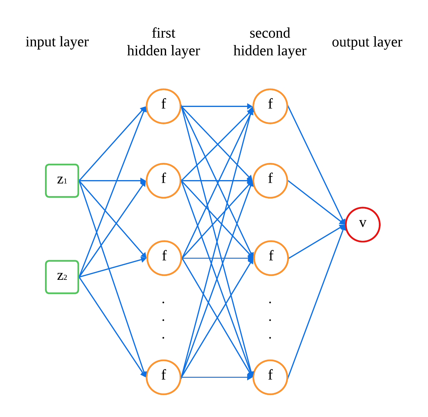
Figure 1: Structure of the FCNN. A neural network with two hidden layers with 64 neurons each and employing the ReLU activation function.

Through training the proposed $15\times 15$ covariance matrix using the FCNN structure depicted in Figure 1, we simulate the remaining covariance matrix for the 33 $H(z)$ CC data points listed in Table 1. The simulated results are presented in Figure 2, where we show two examples of simulated covariance matrices obtained using different hyperparameter configurations. The bottom-left panel corresponds to the simulation with epochs $=500$ and batch size $=10$, while the bottom-right panel corresponds to epochs $=6500$ and batch size $=2$.

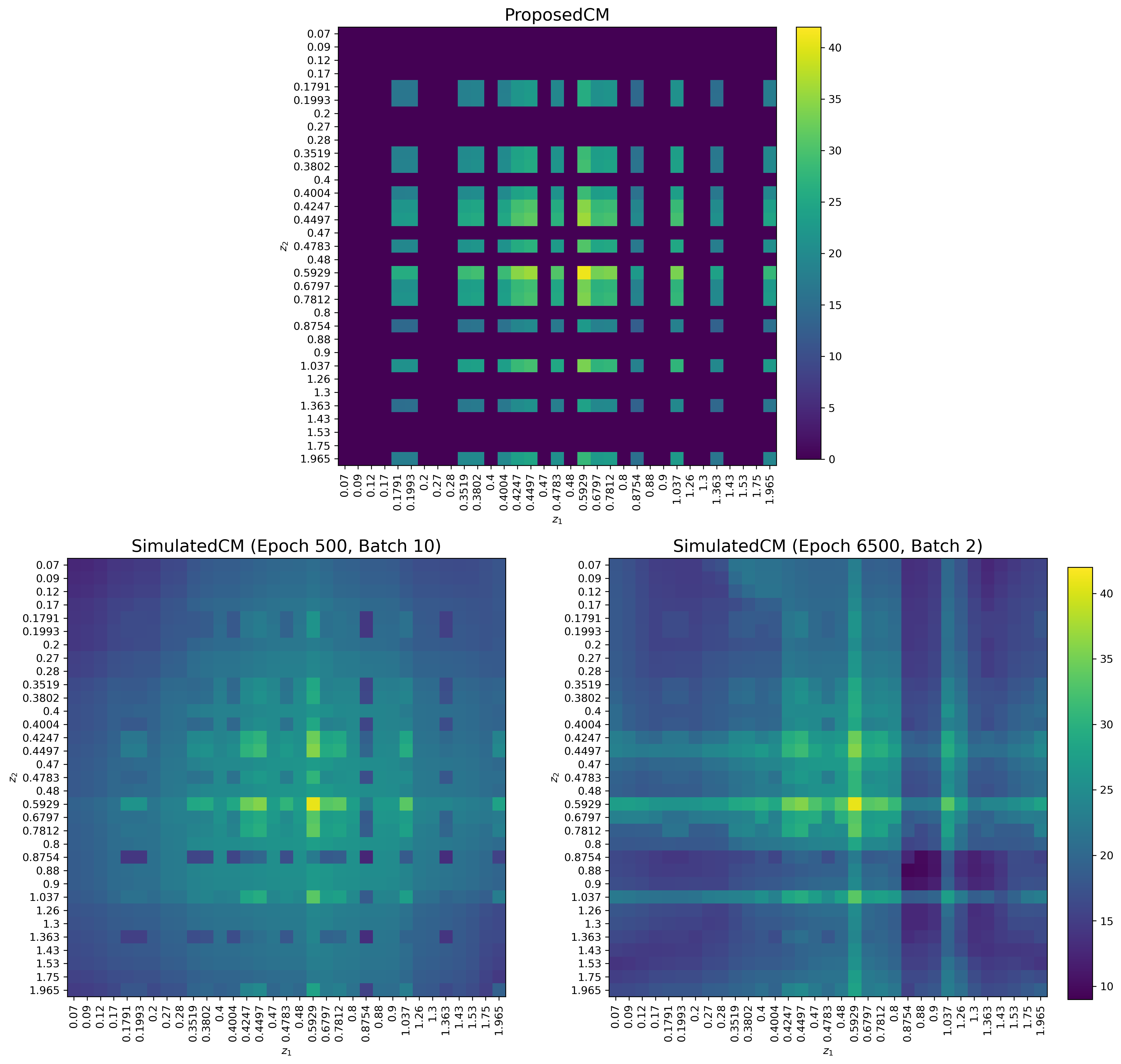
Figure 2: The proposed covariance matrix (top panel) and two simulated covariance matrices (bottom panels). The top panel illustrates the $15\times 15$ covariance matrix proposed by Moresco et al. (2020), where the remaining entries corresponding to the 33 $H(z)$ CC data points listed in Table 1 are assigned a value of 0. The bottom-left and bottom-right panels show two simulated covariance matrices generated using FCNN under different training configurations. Specifically, the bottom-left panel corresponds to a simulation with hyperparameters set to epochs $=500$ and batch size $=10$, while the bottom-right panel corresponds to epochs $=6500$ and batch size $=2$. The x-axis and y-axis labels correspond to the redshift values $z_{1}$ and $z_{2}$, respectively.

From Figure 2, it is clear that the hyperparameters, number of epochs and batch size, have a significant impact on the simulated covariance matrices. However, determining the most accurate configuration remains a challenge. To resolve this, we propose two distinct evaluation criteria to assess the hyperparameter configurations and identify the optimal set. The methodology for this selection process, along with the corresponding simulation results, is detailed in Subsection 4.

4 Selection of Hyperparameters

In FCNN, epochs and batch size are essential hyperparameters for training. An epoch refers to one complete pass through the entire training dataset. Training typically involves multiple epochs to minimize the loss function, with the number chosen to balance underfitting and overfitting. The batch size specifies the number of training samples processed together in a single forward and backward pass. It influences the stability of gradient updates and the efficiency of training. The choice of batch size and epochs together determines the total weight updates during training, affecting convergence and performance.

In Subsection 3, we demonstrate that the hyperparameters, namely epochs and batch size, play a critical role in shaping the simulated covariance matrix using the FCNN. In this subsection, we propose two criteria for evaluating and selecting the optimal hyperparameter configuration to enhance the simulation.

The first criterion, presented in Subsubsection 4.1, involves calculating the loss, validation loss (valloss), and their average $(\text{loss}+\text{valloss})/2$ for each combination of epochs and batch size, where smaller values indicate a better configuration. The second criterion, explained in Subsubsection 4.2, introduces an inverse test based on the $\chi^{2}$ statistic. This test evaluates the effectiveness of different combinations of epochs and batch size in simulating the covariance matrix using the FCNN, helping identify the most suitable configuration.

4.1 Criterion 1: loss, valloss, and $(loss+valloss)/2$

The loss metric evaluates the model’s performance on the training dataset, while valloss assesses its generalization capability on the validation dataset. An increasing valloss alongside a decreasing loss typically indicates overfitting, whereas consistently high loss and valloss suggest underfitting. In this paper, the dataset is split into a training-to-validation ratio of 9:1 to balance model training and validation. These metrics are essential for tuning the combination of epochs and batch size, enabling the selection of the optimal configuration from numerous possibilities to collectively optimize model performance and enhance generalization.

The loss and valloss metrics used in this paper are both computed as the average squared error (MSE), with loss calculated over the training dataset and valloss over the validation dataset, defined as:

$$\text{loss}=\frac{1}{N}\sum_{i=1}^{N}(v_{i}-\hat{v}_{i})^{2},$$ (11)

$$\text{valloss}=\frac{1}{M}\sum_{j=1}^{M}(v_{j}-\hat{v}_{j})^{2},$$ (12)

where $N$ and $M$ are the numbers of samples in the training and validation datasets, respectively, $v_{i}$ and $v_{j}$ are the true labels, and $\hat{v}_{i}$ and $\hat{v}_{j}$ are the predicted outputs. While this paper focuses on MSE, other loss functions, such as Cross-Entropy Loss or Huber Loss, can be used depending on the problem and dataset.

To select the optimal combination of epochs and batch size for simulating the covariance matrix, we evaluate the loss and valloss for each combination of $\text{epochs}\in[500,7000]$ with an interval of 500, and $\text{batch size}\in[2,28]$ with an interval of 2. Since the results can vary slightly each time the code is executed with the same hyperparameters, we repeat each combination 10 times and compute the mean loss and valloss to minimize the influence of randomness. To account for both loss and valloss simultaneously, we also compute their mean as $(\text{loss}+\text{valloss})/2$. The results are illustrated in Figure 3 and summarized in Table 2. They indicate that for loss, valloss, and $(\text{loss}+\text{valloss})/2$, the optimal combinations of epochs and batch size are highly similar. Specifically, the optimal number of epochs is consistently 6500. For batch size, the optimal value is 2 for loss and $(\text{loss}+\text{valloss})/2$, while it is 4 for valloss. This consistency highlights the similar behavior of these metrics when determining the optimal training configuration.

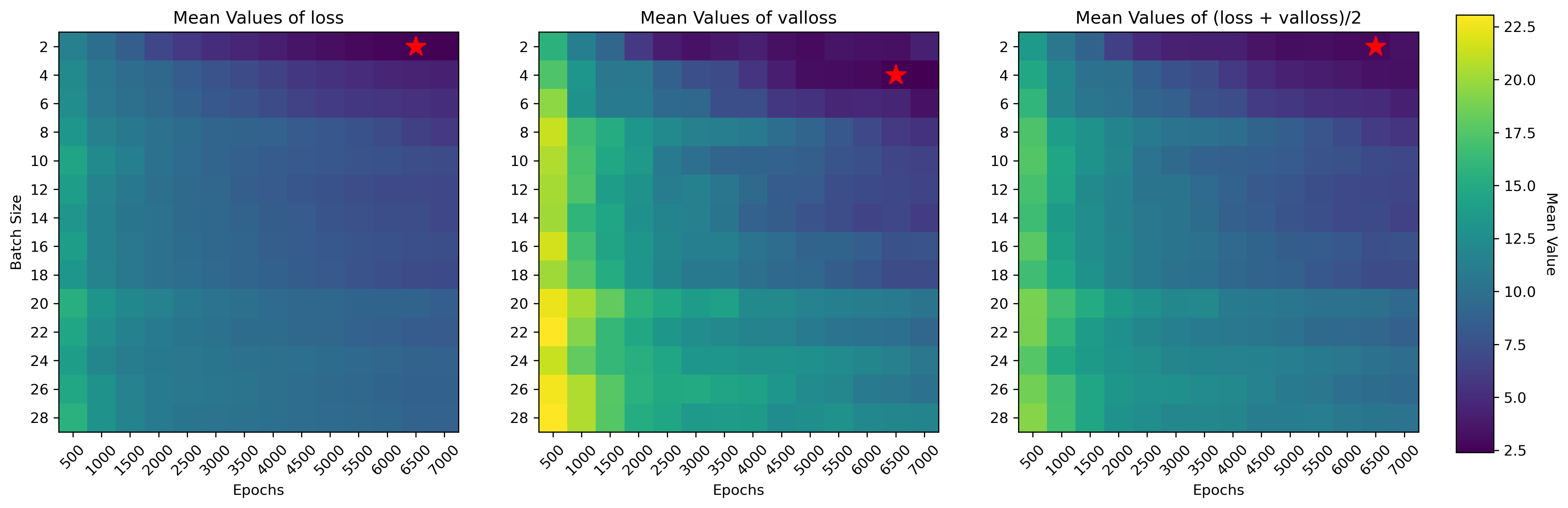
Figure 3: Heatmaps of the mean values of loss, valloss, and $(\text{loss}+\text{valloss})/2$ for an FCNN using different combinations of epochs and batch sizes. The red star in each subplot marks the position of the minimum value, representing the optimal combination of epochs and batch size.

Criteria	Epoch	Batch Size	$\textbf{H}_{0}$ with SCM
loss	6500	2	EMCEE	$67.65\pm 5.26$
			GP	$68.25\pm 5.96$
valloss	6500	4	EMCEE	$67.70\pm 5.25$
			GP	$68.35\pm 5.98$
(loss + valloss)/2	6500	2	EMCEE	$67.65\pm 5.26$
			GP	$68.25\pm 5.96$
$\chi^{2}$	7000	18	EMCEE	$67.70\pm 5.28$
			GP	$68.65\pm 6.08$

Table 2: Optimal combinations of epochs and batch sizes for different criteria, along with the constrained $\mathrm{H}_{0}$ values obtained using EMCEE and GP methods with the simulated covariance matrix (SCM).

4.2 Criterion 2: inversed test based on $\chi^{2}$

To minimize the influence of specific criteria in evaluating optimal hyperparameters such as epochs and batch size, we propose a novel inversed test based on $\chi^{2}$. In this method, the FCNN first generates an extended covariance matrix from the proposed one. The FCNN is then used again to reconstruct a new matrix at the original positions of the proposed covariance matrix. By comparing this reconstructed matrix to the original using a chi-squared metric, the method directly assesses the network’s ability to preserve the statistical properties of the data. This approach is particularly useful for evaluating and selecting the hyperparameters of the FCNN because the $\chi^{2}$ metric provides a quantitative and objective measure of how accurately the network reconstructs the covariance matrix. By minimizing the $\chi^{2}$ value, the method ensures that the chosen hyperparameters lead to reliable simulations, reducing variability and enhancing the network’s overall performance. The procedure is illustrated in Figure 4 and detailed as follows:

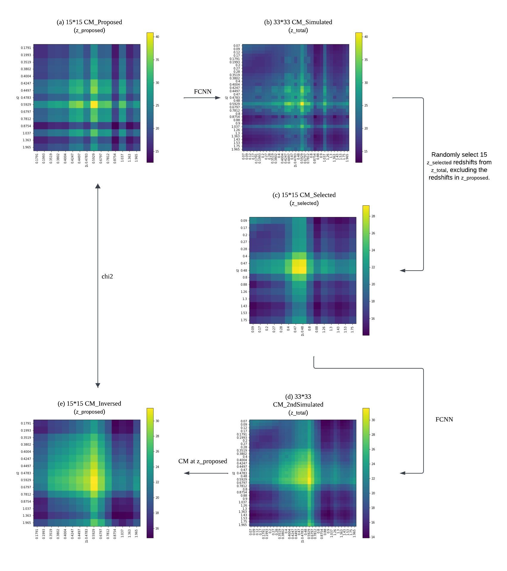
Figure 4: The procedure of the inversed test based on $\chi^{2}$ with hyperparameters, epochs = 7000 and batch size = 18.

• Step 1: Simulating the Full Covariance Matrix
  The covariance matrix $\text{CM}_{\text{Simulated}}$ is generated from the proposed covariance matrix $\text{CM}_{\text{Proposed}}$ using FCNN with a specific combination of hyperparameters (epochs and batch size).

• Step 2: Selecting Additional Redshifts
  Randomly select the same number of redshifts as in $\text{CM}_{\text{Proposed}}$, denoted as $z_{\text{selected}}$, ensuring that the selected redshifts exclude those in $z_{\text{proposed}}$. This exclusion is crucial to create an independent and unbiased test of the FCNN’s simulation process, preventing circular validation and testing the model’s ability to generalize to new redshifts. The corresponding covariance matrix for $z_{\text{selected}}$ is $\text{CM}_{\text{Selected}}$.

• Step 3: Simulating the Second Covariance Matrix
  The covariance matrix $\text{CM}_{\text{2ndSimulated}}$ is simulated using the FCNN, based on the newly selected redshifts and their associated covariance matrix $\text{CM}_{\text{Selected}}$.

• Step 4: Extracting and Comparing Covariance Matrices
  Extract the covariance matrix at the redshift positions $z_{\text{proposed}}$ from $\text{CM}_{\text{2ndSimulated}}$, denoted as $\text{CM}_{\text{Inversed}}$. Compute the $\chi^{2}$ value between $\text{CM}_{\text{Inversed}}$ and the original $\text{CM}_{\text{Proposed}}$ to assess the agreement.

• Step 5: Reducing Variability with Multiple Simulations
  Since FCNN simulations introduce slight variations, repeat Steps 1 through 4 ten times to mitigate their impact. Calculate the mean $\chi^{2}$ over these iterations for each combination of hyperparameters (epochs and batch size). The final results, showcasing the minimum mean $\chi^{2}$ values, are presented in Figure 5.

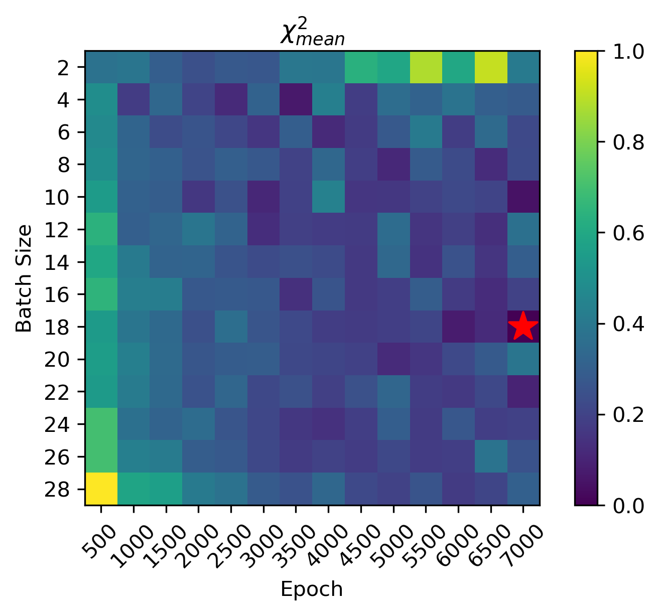
Figure 5: The heatmap of $\chi^{2}_{\text{mean}}$ between $\text{CM}_{\text{Iversed}}$ and $\text{CM}_{\text{Proposed}}$ for different hyperparameter combinations of epochs and batch size. The red star marks the position of the minimum value, representing the optimal combination.

Based on the criterion of the inversed test with $\chi^{2}$, Figure 5 demonstrates that the optimal combination of hyperparameters is epochs = 7000 and batch size = 18, as detailed in Table 2. From Table 2, it can be observed that the optimal number of epochs is consistent across different criteria, indicating that the choice of criterion does not significantly affect the optimal epochs. However, the optimal batch size for the $\chi^{2}$ based inversed test differs from that of other criteria.

5 Constraining $\mathrm{H}_{0}$ Using the CC Dataset

To examine how different combinations of hyperparameters influence the constrained $\mathrm{H}_{0}$, we use the CC dataset listed in Table 1 together with the simulated covariance matrix to perform the constraint on $\mathrm{H}_{0}$. The simulated covariance matrix is created by the FCNN, based on the proposed covariance matrix. Different combinations of hyperparameters, determined by various criteria, are used in the FCNN to generate the simulated covariance matrix. To minimize the influence of the chosen constraint method on the $\mathrm{H}_{0}$ results derived from the CC dataset with a simulated covariance matrix, this research employs two complementary approaches: the EMCEE and the GP.

5.1 EMCEE

In this Subsection, we utilize the EMCEE to constrain the Hubble constant, $\mathrm{H}_{0}$, based on the CC dataset while incorporating a covariance matrix to account for correlations between data points. This approach ensures robust and reliable parameter estimation. To model the relationship between the Hubble parameter, $H(z)$, and the cosmological parameters, we adopt the flat $\Lambda$CDM cosmological model. The corresponding Friedmann equation is expressed as:

$$H(z)=\mathrm{H}_{0}\sqrt{\Omega_{M}(1+z)^{3}+(1-\Omega_{M})},$$ (13)

where $H(z)$ represents the Hubble parameter at redshift $z$, $\mathrm{H}_{0}$ is the Hubble constant, and $\Omega_{M}$ is the matter density parameter.

The CC dataset provides the observational values $H_{\mathrm{obs}}(z)$, their associated uncertainties $\sigma_{\mathrm{obs}}$, and the redshift values $z$. Additionally, the covariance matrix $\mathrm{Cov}$ accounts for the correlations between these observations. To constrain $\mathrm{H}_{0}$ and $\Omega_{M}$, we employ Bayes’ theorem, which expresses the relationship between the posterior probability of the parameters, the likelihood of the observed data, and the prior distribution:

$$P(\mathrm{H_{0},\Omega_{M}}|H_{\mathrm{obs}})=\frac{P(H_{\mathrm{obs}}|\mathrm{H_{0},\Omega_{M}})P(\mathrm{H_{0},\Omega_{M}})}{P(H_{\mathrm{obs}})},$$ (14)

where $P(H_{\mathrm{obs}}|\mathrm{H}_{0},\Omega_{M})$ is the likelihood function, which quantifies the probability of obtaining the observed data given specific values of $\mathrm{H}_{0}$ and $\Omega_{M}$. The term $P(\mathrm{H}_{0},\Omega_{M})$ represents the prior distribution, encapsulating prior knowledge or assumptions about these parameters before considering the data. The denominator, $P(H_{\mathrm{obs}})$, known as the evidence or marginal likelihood, serves as a normalization factor to ensure that the posterior probability $P(\mathrm{H}_{0},\Omega_{M}|H_{\mathrm{obs}})$ is properly scaled.

The likelihood function is expressed as (Ma & Zhang, 2011; Wang et al., 2021):

$$\mathcal{L}=\exp{\left(-\frac{1}{2}\chi^{2}\right)},$$ (15)

where the $\chi^{2}$ statistic quantifies the goodness of fit between the model and the observations. The $\chi^{2}$ is defined as:

$$\chi^{2}=\bm{r}^{T}\,\mathrm{Cov}^{-1}\,\bm{r},$$ (16)

with the residual vector $\bm{r}$ given by:

$$r_{i}=H_{\mathrm{obs},i}-H_{\mathrm{model},i}.$$ (17)

Here, $H_{\mathrm{obs},i}$ and $H_{\mathrm{model},i}$ are the observed and model-predicted Hubble parameter values, respectively, and $\mathrm{Cov}^{-1}$ is the inverse of the covariance matrix. This formulation ensures that the $\chi^{2}$ accounts for both the individual variances and the correlations between the observations.

Using EMCEE, we sample the posterior distribution of $\mathrm{H}_{0}$ and $\Omega_{M}$ to derive their constraints, effectively incorporating the effects of the covariance matrix into the analysis. This method provides robust and statistically rigorous estimates of the parameters. To analyze the influence of different optimal combinations of hyperparameters—epochs and batch size—on constraining $\mathrm{H}_{0}$, we first use FCNN to simulate the covariance matrix based on these combinations. Then, we apply the simulated covariance matrix along with the CC dataset to constrain $\mathrm{H}_{0}$ using EMCEE. The optimal combinations of epochs and batch size used are listed in Table 2. To reduce the impact of randomness in the simulation, we generate the covariance matrix 10 times, constraining $\mathrm{H}_{0}$ in each instance. We then compute the mean of these 10 constrained values, with the results presented in Table 2.

From Table 2, we observe that the optimal combinations of epochs and batch size for different criteria have little influence on the constrained $\mathrm{H}_{0}$, as the results are similar across different combinations. This indicates that although the criteria for selecting the optimal combinations of epochs and batch size differ, and the resulting combinations themselves vary, the choice of criteria does not significantly impact the constrained $\mathrm{H}_{0}$. Additionally, we compute the constrained $\mathrm{H}_{0}$ for another combination, specifically epochs $=500$ and batch size $=28$, yielding $\mathrm{H}_{0}=67.00\pm 5.35$. This value differs significantly from the constrained $\mathrm{H}_{0}$ obtained using the optimal combinations listed in Table 2, highlighting the necessity of selecting appropriate epochs and batch size combinations when constraining $\mathrm{H}_{0}$. Furthermore, we calculate $\mathrm{H}_{0}=67.86\pm 3.08$ when no covariance matrix is used and $\mathrm{H}_{0}=69.14\pm 4.10$ when incorporating the proposed $15\times 15$ covariance matrix. Compared to the constrained $\mathrm{H}_{0}$ values in Table 2, which are obtained using optimal epochs and batch size combinations, these results exhibit a smaller $1\sigma$ uncertainty. This indicates that introducing a simulated covariance matrix into the CC dataset increases the uncertainty in the constrained $\mathrm{H}_{0}$. Moreover, the proposed covariance matrix further increases the $1\sigma$ uncertainty compared to the case where no covariance matrix is used. Overall, these findings indicate that neglecting the covariance matrix in the CC dataset when constraining $\mathrm{H}_{0}$ leads to an underestimation of the $1\sigma$ uncertainty. Moreover, while the choice of epochs and batch size combinations is crucial for simulating the covariance matrix, the specific criteria used for selecting these combinations have only a minor impact on constraining $\mathrm{H}_{0}$.

5.2 GP

In Subsection 5.1, we examine how different combinations of epochs and batch size affect the constraint on $\mathrm{H}_{0}$. This is done by simulating the covariance matrix of the CC dataset and applying the EMCEE method. To minimize the impact of the constraint method itself, we take a different approach in this subsection. Instead of using EMCEE, we apply Gaussian Process to test how different epoch and batch size combinations in FCNN-based covariance matrix simulations influence the $\mathrm{H}_{0}$ constraint.

GP regression provides a model-independent method for reconstructing the CC dataset and estimating $\mathrm{H}_{0}$. Following Rasmussen & Williams (2006), GP is a non-parametric approach that models data as a multivariate Gaussian distribution, enabling the interpolation of unknown values without assuming an explicit functional form. This makes it particularly useful for reconstructing the Hubble parameter $H(z)$ as a function of redshift $z$, where $\mathrm{H}_{0}$ is determined from the reconstructed value of $H(z)$ at $z=0$. In this study, we enhance the standard GP approach by incorporating the full covariance matrix of the CC dataset, which is simulated using an FCNN. Unlike previous studies (Sun et al., 2021; Zhang et al., 2023) that assumed independent data points with only diagonal uncertainties, our approach effectively captures correlations between redshift measurements. This provides a more comprehensive statistical treatment of the data and improves the robustness of the resulting $\mathrm{H}_{0}$ constraint.

To model the observed CC data, given as ($z_{i},H_{i},\sigma_{i}$), we assume that the errors $\sigma_{i}$ follow a Gaussian distribution. The data vector $\bm{H}$ is then described by

$$\bm{H}\sim\mathcal{N}(\bm{\mu},K(\bm{Z},\bm{Z})+C),$$ (18)

where $\mathcal{N}$ represents a Gaussian Process, $\bm{\mu}$ is the mean function, and $K(\bm{Z},\bm{Z})$ is the covariance function that captures the relationships between data points. Here, $C$ is the full covariance matrix of the CC dataset, which accounts for both statistical and systematic uncertainties. It is defined in Equation (2). The covariance between two data points, $H(z_{i})$ and $H(z_{j})$, is given by a covariance function, also known as a kernel. There are multiple choices for the kernel function (Zhang et al., 2023), but in this study, we adopt the widely used Squared Exponential covariance function (Seikel et al., 2012; Wang et al., 2021; Sun et al., 2021)

$$k(z_{i},z_{j})=\sigma^{2}_{f}\exp{\left(-\frac{(z_{i}-z_{j})^{2}}{2l^{2}}\right)},$$ (19)

where $l$ is the characteristic length scale controlling the smoothness of the function, and $\sigma_{f}$ is the signal variance determining the amplitude of the fluctuations. These hyperparameters are optimized during the GP fitting process.

To extend the GP model to new redshift points $\bm{Z^{\ast}}$, we define a corresponding Gaussian vector

$$\bm{f^{\ast}}\sim\mathcal{N}(\bm{\mu^{\ast}},K(\bm{Z^{\ast}},\bm{Z^{\ast}})).$$ (20)

Combining Equations (18) and (20) in a joint Gaussian distribution (Seikel et al., 2012), we obtain

$$\begin{bmatrix}\bm{H}\\ \bm{f^{\ast}}\\ \end{bmatrix}\sim\mathcal{N}\left(\begin{bmatrix}\bm{\mu}\\ \bm{\mu^{\ast}}\\ \end{bmatrix},\begin{bmatrix}K(\bm{Z},\bm{Z})+C&K(\bm{Z},\bm{Z^{\ast}})\\ K(\bm{Z^{\ast}},\bm{Z})&K(\bm{Z^{\ast}},\bm{Z^{\ast}})\\ \end{bmatrix}\right).$$ (21)

From this, we derive the mean and covariance of the reconstructed function (Rasmussen & Williams, 2006; Seikel et al., 2012)

$$\bm{\bar{f^{\ast}}}=\bm{\mu^{\ast}}+K(\bm{Z^{\ast}},\bm{Z})[K(\bm{Z},\bm{Z})+C]^{-1}(\bm{H}-\bm{\mu}),$$ (22)

$$\begin{split}\operatorname{cov}(\bm{f^{\ast}})&=K(\bm{Z^{\ast}},\bm{Z})-K(\bm{Z^{\ast}},\bm{Z})[K(\bm{Z},\bm{Z})+C]^{-1}\\ &\quad-K(\bm{Z},\bm{Z^{\ast}}).\end{split}$$ (23)

The hyperparameters $l$ and $\sigma_{f}$ are determined by maximizing the log marginal likelihood

$$\begin{split}\ln\mathcal{L}&=-\frac{1}{2}(\bm{H}-\bm{\mu})^{T}[K(\bm{Z},\bm{Z})+C]^{-1}(\bm{H}-\bm{\mu})\\ &\quad-\frac{1}{2}\ln|K(\bm{Z},\bm{Z})+C|-\frac{n}{2}\ln 2\pi.\end{split}$$ (24)

Following this procedure, we reconstruct $H(z)$ and obtain $\mathrm{H}_{0}$ by evaluating the reconstructed function at $z=0$. For implementation, we use the Gaussian process regression package GAPP (Gaussian Processes in Python) developed by Seikel et al. (2012). The inclusion of the full covariance matrix provides an improved statistical treatment and leads to a more robust constraint on $\mathrm{H}_{0}$ from the CC dataset.

To further evaluate the impact of different optimal combinations of epochs and batch size on constraining $\mathrm{H}_{0}$, we perform an additional test using Gaussian Process regression. While the previous analysis used EMCEE for constraint estimation, here we adopt GP to examine whether the choice of constraint method affects the influence of the simulated covariance matrix on $\mathrm{H}_{0}$. Following the same procedure as in the EMCEE test, we first use FCNN to generate the covariance matrix based on different epoch and batch size combinations. The optimal combinations used are listed in Table 2. To mitigate the impact of randomness, we simulate the covariance matrix 10 times and apply GP regression in each case to obtain $\mathrm{H}_{0}$. The mean values of these constraints are reported in Table 2, allowing for a direct comparison with the results obtained using EMCEE.

From Table 2, GP consistently yields higher $\mathrm{H}_{0}$ values than EMCEE across all selection criteria, with slightly larger uncertainties. For example, under the loss criterion, GP gives $\mathrm{H}_{0}=68.25\pm 5.96$, while EMCEE gives $\mathrm{H}_{0}=67.65\pm 5.26$. A similar trend is observed for other criteria, indicating that the choice of constraint method affects the constrained $\mathrm{H}_{0}$ when using the simulated covariance matrix within the CC dataset. For the alternative setting (epochs $=500$, batch size $=28$), GP yields $\mathrm{H}_{0}=67.17\pm 6.13$, deviating from the optimal settings, which aligns with the EMCEE findings and highlights the importance of carefully selecting epochs and batch size. Regarding the covariance matrix, GP results in $\mathrm{H}_{0}=67.76\pm 4.78$ when no covariance matrix is used and $\mathrm{H}_{0}=67.22\pm 4.72$ when incorporating the proposed $15\times 15$ covariance matrix. Unlike EMCEE, where including the proposed covariance matrix increases uncertainty, GP’s uncertainties remain similar in both cases. However, compared to the full simulated covariance matrix case, both methods show smaller uncertainties, suggesting that the proposed covariance matrix contributes to an intermediate level of error propagation.

These results demonstrate several consistent findings between EMCEE and GP. First, for both methods, different selection criteria for epoch and batch size have little influence on the constrained $\mathrm{H}_{0}$, as the values remain stable across different combinations. Second, the inclusion of the simulated covariance matrix increases the overall uncertainty in the constrained $\mathrm{H}_{0}$, regardless of whether EMCEE or GP is used. However, differences between the two methods are also observed. While EMCEE exhibits increased uncertainty when incorporating the proposed covariance matrix, GP’s uncertainties remain nearly unchanged. Additionally, GP systematically yields higher $\mathrm{H}_{0}$ values than EMCEE across all selection criteria, indicating that the constraint method itself influences the final results. These findings suggest that both the choice of constraint method and the treatment of the covariance matrix play a role in shaping the constrained $\mathrm{H}_{0}$, highlighting the need for careful methodological considerations when interpreting results.

6 Conclusion

In this study, we investigated the impact of incorporating a simulated covariance matrix on constraining the Hubble constant, $\mathrm{H}_{0}$, using the CC dataset. Recognizing that previous studies either neglected off-diagonal elements (Niu & Zhang, 2023; Zhang et al., 2023) or used an incomplete covariance matrix (Zhang et al., 2024; Niu et al., 2024), we addressed this gap by employing FCNN to simulate the full $33\times 33$ covariance matrix. Since the full covariance matrix of the CC dataset has not been explicitly proposed, we based our simulation on the $15\times 15$ covariance matrix from Moresco et al. (2020). This simulation is grounded in the assumption that the covariance matrix follows a generalizable pattern that the FCNN can learn (see Subsection 3).

During the simulation of the covariance matrix, we observed that the combination of two key hyperparameters, epochs and batch size, significantly influenced the simulation results (Subsection 3). To address this issue, we systematically investigated their impact by proposing and testing two evaluation criteria: (1) minimizing loss and validation loss, and (2) an inverse test based on the chi-squared statistic (Subsections 4.1 and 4.2). Our results indicate that different selection criteria lead to variations in the chosen hyperparameter combinations, but they have little impact on the constrained $\mathrm{H}_{0}$ (see Table 2). However, the specific combination of epochs and batch size does have a substantial effect on the final constrained $\mathrm{H}_{0}$. For example, using epochs $=500$ and batch size $=28$ led to a noticeably different $\mathrm{H}_{0}$ compared to the optimal hyperparameter selections, highlighting the importance of carefully tuning hyperparameters when applying FCNN-based simulations to scientific datasets (see Section 5).

To evaluate the effect of different hyperparameter combinations on the constrained $\mathrm{H}_{0}$, we employed two independent methods: the EMCEE (Subsection 5.1) and Gaussian Process (Subsection 5.2). This allowed us to determine how the choice of hyperparameters in the FCNN-simulated covariance matrix influences the constrained $\mathrm{H}_{0}$. The results show that different hyperparameter selection criteria for the FCNN have little impact on the constrained $\mathrm{H}_{0}$, but different epoch and batch size combinations do significantly affect it (Table 2). Additionally, incorporating the simulated covariance matrix into the CC dataset generally increases the uncertainty of the constrained $\mathrm{H}_{0}$ compared to cases where no covariance matrix or only the proposed $15\times 15$ covariance matrix is used. Furthermore, we observed that GP consistently yields slightly higher values of $\mathrm{H}_{0}$ than EMCEE, suggesting that the constraint method itself influences the final results. This underscores the necessity of selecting appropriate methodologies when using covariance matrices in $\mathrm{H}_{0}$ constraints.

Future work can improve upon this study in several ways. (1) Exploring more advanced neural network architectures could enhance the accuracy of covariance matrix simulations. (2) Increasing the number of observational data points in the CC dataset could lead to more precise covariance matrix simulations and better constraints on $\mathrm{H}_{0}$. (3) Directly measuring $H(z)$ with an observationally derived covariance matrix rather than relying on a simulated one would allow for a direct comparison to validate the ANN-based approach. (4) Further studies should refine the assumptions behind the covariance matrix simulation, such as testing whether the FCNN is truly learning a valid underlying pattern and exploring alternative statistical methods for inferring missing correlations. These improvements will help refine $\mathrm{H}_{0}$ constraints and enhance our understanding of cosmic expansion.

Appendix A Correction of the Hubble Parameter at $z=0.09$

The Hubble parameter at redshift $z=0.09$ is often reported as $H(0.09)=69\pm 12\,\mathrm{km\,s^{-1}\,Mpc^{-1}}$ in numerous studies (Moresco, 2023; Niu et al., 2024). The original source of this data point is Jimenez et al. (2003), where $69\pm 12\,\mathrm{km\,s^{-1}\,Mpc^{-1}}$ is used as an estimate of the Hubble constant $\mathrm{H}_{0}$. To accurately obtain the Hubble parameter at redshift $z=0.09$, we must adjust this value using the cosmological model parameters provided in that study, as follows

$$H(z)=H_{0}\sqrt{\Omega_{M}(1+z)^{3}+\Omega_{\Lambda}},$$ (A1)

where $H_{0}=69\pm 12\,\mathrm{km\,s^{-1}\,Mpc^{-1}}$ is the Hubble constant, $\Omega_{M}=0.27$ is the matter density parameter, and $\Omega_{\Lambda}=0.7$ is the dark energy density parameter.

To determine the $1\sigma$ uncertainty in $H(0.09)$, we apply uncertainty propagation. For a general function $f=f(x_{1},x_{2},\ldots,x_{n})$, the variance is given by

$$\sigma_{f}^{2}=\sum_{i=1}^{n}\left(\frac{\partial f}{\partial x_{i}}\right)^{2}\sigma_{i}^{2}+\sum_{i=1}^{n}\sum_{j\neq i}^{n}\frac{\partial f}{\partial x_{i}}\frac{\partial f}{\partial x_{j}}\sigma_{ij},$$ (A2)

where $\sigma_{i}$ is the standard deviation of $x_{i}$, and $\sigma_{ij}$ represents the covariance between the variables $x_{i}$ and $x_{j}$. The covariance $\sigma_{ij}$ is calculated as

$$\sigma_{ij}=\frac{1}{N}\sum_{k=1}^{N}(x_{ik}-\bar{x_{i}})(y_{jk}-\bar{y_{j}}),$$ (A3)

where $x_{ik}$ is the $k$-th value of $x_{i}$, and $N$ is the total number $k$. Based on Equation (A2), the propagated uncertainty in $H(z)$ is given by

$$\sigma_{H(z)}=\sqrt{\Omega_{M}(1+z)^{3}+\Omega_{\Lambda}}\cdot\sigma_{H_{0}}.$$ (A4)

According to Equations (A1) and (A4), we obtain the updated value for the Hubble parameter at $z=0.09$ as $H(0.09)=70.7\pm 12.3\,\mathrm{km\,s^{-1}\,Mpc^{-1}}$.

References

- Alam et al. (2017) Alam, S., Ata, M., Bailey, S., et al. 2017, MNRAS, 470, 2617, doi: 10.1093/mnras/stx721
- Eisenstein et al. (2005) Eisenstein, D. J., Zehavi, I., Hogg, D. W., et al. 2005, ApJ, 633, 560, doi: 10.1086/466512
- Foreman-Mackey et al. (2013) Foreman-Mackey, D., Hogg, D. W., Lang, D., & Goodman, J. 2013, PASP, 125, 306, doi: 10.1086/670067
- Jiao et al. (2023) Jiao, K., Borghi, N., Moresco, M., & Zhang, T.-J. 2023, ApJS, 265, 48, doi: 10.3847/1538-4365/acbc77
- Jimenez & Loeb (2002) Jimenez, R., & Loeb, A. 2002, ApJ, 573, 37, doi: 10.1086/340549
- Jimenez et al. (2003) Jimenez, R., Verde, L., Treu, T., & Stern, D. 2003, ApJ, 593, 622, doi: 10.1086/376595
- Ma & Zhang (2011) Ma, C., & Zhang, T.-J. 2011, ApJ, 730, 74, doi: 10.1088/0004-637X/730/2/74
- Mcculloch & Pitts (1943) Mcculloch, W., & Pitts, W. 1943, Bulletin of Mathematical Biophysics, 5, 115–133
- Moresco (2015) Moresco, M. 2015, MNRAS, 450, L16, doi: 10.1093/mnrasl/slv037
- Moresco (2023) —. 2023, arXiv e-prints, arXiv:2307.09501, doi: 10.48550/arXiv.2307.09501
- Moresco et al. (2020) Moresco, M., Jimenez, R., Verde, L., Cimatti, A., & Pozzetti, L. 2020, ApJ, 898, 82, doi: 10.3847/1538-4357/ab9eb0
- Moresco et al. (2018) Moresco, M., Jimenez, R., Verde, L., et al. 2018, ApJ, 868, 84, doi: 10.3847/1538-4357/aae829
- Moresco et al. (2012) Moresco, M., Cimatti, A., Jimenez, R., et al. 2012, J. Cosmology Astropart. Phys, 2012, 006, doi: 10.1088/1475-7516/2012/08/006
- Moresco et al. (2016) Moresco, M., Pozzetti, L., Cimatti, A., et al. 2016, J. Cosmology Astropart. Phys, 2016, 014, doi: 10.1088/1475-7516/2016/05/014
- Niu et al. (2024) Niu, J., Jiao, K., He, P., & Zhang, T.-J. 2024, ApJ, 972, 14, doi: 10.3847/1538-4357/ad5fef
- Niu & Zhang (2023) Niu, J., & Zhang, T.-J. 2023, Physics of the Dark Universe, 39, 101147, doi: 10.1016/j.dark.2022.101147
- Perlmutter et al. (1999) Perlmutter, S., Aldering, G., Goldhaber, G., et al. 1999, ApJ, 517, 565, doi: 10.1086/307221
- Planck Collaboration et al. (2020) Planck Collaboration, Aghanim, N., Akrami, Y., et al. 2020, A&A, 641, A6, doi: 10.1051/0004-6361/201833910
- Rasmussen & Williams (2006) Rasmussen, C. E., & Williams, C. K. I. 2006, Gaussian Processes for Machine Learning
- Ratsimbazafy et al. (2017) Ratsimbazafy, A. L., Loubser, S. I., Crawford, S. M., et al. 2017, MNRAS, 467, 3239, doi: 10.1093/mnras/stx301
- Riess (2020) Riess, A. G. 2020, Nature Reviews Physics, 2, 10, doi: 10.1038/s42254-019-0137-0
- Riess et al. (1998) Riess, A. G., Filippenko, A. V., Challis, P., et al. 1998, AJ, 116, 1009, doi: 10.1086/300499
- Riess et al. (2022) Riess, A. G., Yuan, W., Macri, L. M., et al. 2022, ApJ, 934, L7, doi: 10.3847/2041-8213/ac5c5b
- Seikel et al. (2012) Seikel, M., Clarkson, C., & Smith, M. 2012, J. Cosmology Astropart. Phys, 2012, 036, doi: 10.1088/1475-7516/2012/06/036
- Simon et al. (2005) Simon, J., Verde, L., & Jimenez, R. 2005, Phys. Rev. D, 71, 123001, doi: 10.1103/PhysRevD.71.123001
- Stern et al. (2010) Stern, D., Jimenez, R., Verde, L., Kamionkowski, M., & Stanford, S. A. 2010, J. Cosmology Astropart. Phys, 2010, 008, doi: 10.1088/1475-7516/2010/02/008
- Sun et al. (2021) Sun, W., Jiao, K., & Zhang, T.-J. 2021, ApJ, 915, 123, doi: 10.3847/1538-4357/ac05b8
- Tomasetti et al. (2023) Tomasetti, E., Moresco, M., Borghi, N., et al. 2023, A&A, 679, A96, doi: 10.1051/0004-6361/202346992
- Verde et al. (2019) Verde, L., Treu, T., & Riess, A. G. 2019, Nature Astronomy, 3, 891, doi: 10.1038/s41550-019-0902-0
- Wang et al. (2021) Wang, Y.-C., Xie, Y.-B., Zhang, T.-J., et al. 2021, ApJS, 254, 43, doi: 10.3847/1538-4365/abf8aa
- Zhang et al. (2014) Zhang, C., Zhang, H., Yuan, S., et al. 2014, Research in Astronomy and Astrophysics, 14, 1221, doi: 10.1088/1674-4527/14/10/002
- Zhang et al. (2023) Zhang, H., Wang, Y.-C., Zhang, T.-J., & Zhang, T. 2023, ApJS, 266, 27, doi: 10.3847/1538-4365/accb92
- Zhang et al. (2024) Zhang, J.-C., Hu, Y., Jiao, K., et al. 2024, ApJS, 270, 23, doi: 10.3847/1538-4365/ad0f1e