An Efficient Row-Based Sparse Fine-Tuning
An Efficient Row-Based Sparse Fine-Tuning
Abstract
Fine-tuning is an important step in adapting foundation models such as large language models to downstream tasks. To make this step more accessible to users with limited computational budgets, it is crucial to develop fine-tuning methods that are memory and computationally efficient. Sparse Fine-tuning (SFT) and Low-rank adaptation (LoRA) are two frameworks that have emerged for addressing this problem and have been adopted widely in practice. In this work, we develop a new SFT framework, based on ideas from neural network pruning. At a high level, we first identify ”important” neurons/nodes using feature importance metrics from network pruning (specifically, we use the structural pruning method), and then perform fine-tuning by restricting to weights involving these neurons. Using experiments on common language tasks, we demonstrate that our method significantly improves the memory efficiency of SFT without increasing training time complexity and implementation complexity, while achieving accuracy comparable to state-of-the-art methods such as LoRA and its variants.
1 Introduction
The paradigm of pre-training followed by fine-tuning has seen tremendous success in the last few years. Very large models (often referred to as foundation models) are first trained, typically using very large amounts of data and computational resources, using self-supervised learning approaches (Dosovitskiy, 2020; Achiam et al., 2023; Dubey et al., 2024; Zhou et al., 2024). When building a model for a new task (which could be a supervised learning task), the idea is to start with the foundation model and then tune its parameters, possibly after adding additional classification layers, by training using task-specific data. The pre-train then fine-tune paradigm has been shown to have significant advantages over training a new model from scratch for the new task. Often, high accuracy can be obtained using much smaller datasets for the new task.
Despite the success, fine-tuning a model with billions of parameters requires access to heavy computational resources, even when the task datasets are fairly small. Fortunately, studies (e.g., (Panigrahi et al., 2023) and references therein) show that fine-tuning only a small fraction of parameters can be effective. Parameter-efficient fine-tuning (PEFT) methods have thus been proposed to carry out this idea and address the challenge of making fine-tuning more accessible (Lialin et al., 2023). A leading PEFT approach, Low-Rank Adaptation (LoRA, Hu et al. 2022), achieves memory efficiency by simply making low-rank updates to the weight matrices in the different layers. Another class of PEFT methods is sparse fine-tuning (SFT, Sung et al. 2021; Guo et al. 2021; Ansell et al. 2022; Nikdan et al. 2024), which learns a sparse matrix, typically an unstructured one, for updating the pre-trained weights. However, SFT typically incurs higher memory costs than LoRA during the fine-tuning process, because of the unstructured sparsity. Several works aim to mitigate the memory complexity of SFT (Mofrad et al., 2019; Holmes et al., 2021; Nikdan et al., 2023, 2024), often at the cost of increased running time and more complex implementations of sparse kernels. Besides PEFTs, techniques like Zeroth-Order optimization (Malladi et al., 2023; Guo et al., 2024b) and quantization (Gholami et al., 2022; Dettmers et al., 2022, 2024) can further enhance memory and training efficiency for fine-tuning, including LoRA and SFT.
As LLMs increase in scale, advancing efficient sparse matrix computation, PEFT, and efficient training remains a crucial problem. Towards this goal, we study the question: Can sparse fine-tuning be improved to create a memory- and parameter-efficient framework, while avoiding additional implementations of sparse operations and without increasing the training time complexity? We answer this question in the affirmative, by proposing a new SFT framework for fine-tuning LLMs and Vision Transformers that achieves memory- and parameter-efficiency while maintaining or even improving performance on downstream tasks. Our approach utilizes NN pruning techniques to identify a subset of fine-tuning parameters and employs a matrix decomposition-based computation for efficient fine-tuning. This design enables the integration of ideas from model compression, SFT, and matrix decomposition methods.
1.1 Our Contributions
At a high level, our contributions are as follows:
-
•
We leverage ideas from network pruning to improve SFT, achieving significant memory efficiency considerably lower than the popular LoRA. Our method uses only standard tensor operations, eliminating the need for custom sparse tensor libraries. Our approach is also modular, and it allows us to integrate several existing pruning techniques (which give different neuron importance scores) and works with all layer types, including LayerNorm and BatchNorm, which LoRA cannot directly handle.
-
•
We analyze the memory assignment of several PEFT methods and suggest that model architecture and computation graphs affect memory more significantly than the number of trainable parameters. We validate our methods across diverse fine-tuning tasks (language and vision) and provide practical guidance on training strategies to maximize efficiency and accuracy.
-
•
We propose two variants of the Taylor importance for different settings in image and language tasks: class-aware Taylor and Zeroth-Order Taylor. The first one is designed for tasks where class-wise accuracy is important (in addition to overall accuracy), such as image classification. Zeroth-Order Taylor is designed for large language models and requires memory only equal to that of a forward pass. In addition, we show how to effectively reduce the estimation variance of the Zeroth-Order estimator.
The rest of the paper is organized as follows. We discuss existing PEFT methods in Section 2 and analyze the existing problem in memory efficiency in Section 3. Following this, we describe our approach in detail in Section 4. Section 5 describes the settings of our experiments. We then present and discuss our results in Section 6. Section 7 concludes with some directions for future work along our lines.
2 Background and Related Work
Parameter-Efficient and Memory-Efficient Fine-Tuning: In various language and vision tasks, the “pre-train then fine-tune” paradigm has been shown highly effective. PEFT methods (Lialin et al., 2023) fine-tune a small subset of the parameters of a large pre-trained model in order to accelerate the training process. We begin by introducing SFT and LoRA, two popular approaches for PEFT.
Sparse Fine-Tuning: SFT formulates the fine-tuning process as learning another weight matrix :
| (1) | |||
| (2) |
where and are the input and output of the hidden layer, respectively, is the forward function, represents the frozen pre-trained parameters, and denotes the final parameters used during inference for the fine-tuning task. The matrix is sparse and is initialized at . Such a decomposition is done for every layer in the neural network. SFT methods try to limit the number of parameters to fine-tune. For selecting non-zero indices, Diff pruning (Guo et al., 2021) learns a mask for (using a standard Backprop algorithm), while FISH Mask (Sung et al., 2021) uses Fisher information to identify important indices in . Lottery Ticket SFT (Ansell et al., 2022) fine-tune the whole model for one epoch, then use itself as an importance score to decide which parameters to fine-tune subsequently. Robust Adaptor (RoSA, Nikdan et al. 2024) combines the above SFTs with LoRA and outperforms all these approaches. However, the key challenge of all SFT methods is that they do not sufficiently reduce memory usage, as keeps the dimensionality of , and thus standard libraries do not yield memory improvements.
Techniques for Efficient Sparse Computation: To reduce memory redundancy in sparse tensor computations, various data formats like compressed sparse column/row (CSC/CSR, Mofrad et al., 2019; Lu et al., 2024) and semi-structured formats (Holmes et al., 2021) have been proposed. These formats enable efficient operations like Sparse Matrix Multiplication (SpMM), which is crucial for dot products and matrix multiplications. Upon these techniques, sparse backpropagation is built to improve training efficiency (Zhang et al., 2020; Gale et al., 2020; Peste et al., 2021; Schwarz et al., 2021; Hoefler et al., 2021; Jiang et al., 2022; Nikdan et al., 2023; Xu et al., 2024). Beyond sparse tensor techniques, NVIDIA also offers memory optimization techniques for efficient training111Available at https://pytorch.org/torchtune/stable/tutorials/memory_optimizations.html.
However, these techniques come with trade-offs, particularly in terms of time complexity and implementation complexity. Achieving memory efficiency often requires a significant increase in time complexity. To mitigate this, some approaches employ optimizations implemented in C++ or lower-level languages, such as those used in (Gale et al., 2020; Nikdan et al., 2023, 2024), to accelerate the training process.
Low-Rank Adaptation (LoRA): Instead of requiring to be sparse, low-rank adaptation aims to find update matrices that are of small rank:
| (3) | |||
| (4) |
where is the LoRA scaling hyper-parameter, are the low-rank matrices with . During inference, the term can be merged into to maintain the inference latency of the original model. During training, owing to the fact that is additive for both the self-attention blocks and the subsequent multilayer perceptron (MLP) layers of transformers (Vaswani, 2017), backpropagation can be performed efficiently for the parameters. Due to LoRA’s simplicity and effectiveness, numerous variants have been proposed to enhance the performance, e.g., QLoRA (Dettmers et al., 2022; Guo et al., 2024a; Li et al., 2024; Dettmers et al., 2024), DoRA (Liu et al., 2024), RoSA (Nikdan et al., 2024), and VeRA (Kopiczko et al., 2024). These methods have achieved exceptional performance, often comparable to full fine-tuning across a range of tasks.
Neural Network Pruning: Besides PEFTs, neural network pruning is another widely applied technique that exploits parameter sparsity to reduce model complexity and speed up inference (LeCun et al., 1989; Han et al., 2015; Han, 2017; Hoefler et al., 2021). Most pruning methods assess importance of neural network weights (or neurons) and remove the least important parameters. Unstructured pruning zeros out individual weights while preserving the network architecture, whereas structured pruning removes parameter groups like channels or neurons, which reduce model size (Liu et al., 2021; Fang et al., 2023; Ma et al., 2023). Both approaches often require retraining to recover lost accuracy during pruning. While effective for classical NNs, pruning LLMs is costly due to high memory demands for computing importance scores and the prohibitive retraining step, making memory-efficient LLM pruning an active research area (Frantar & Alistarh, 2023; Sun et al., 2024).
3 Number of Trainable Parameters Is Not Everything
Before introducing our approach, we want to emphasize that in PEFT research, reducing the number of trainable parameters is not the most critical factor for saving memory. Some PEFT methods mentioned in Section 2 focus on reducing the number of trainable parameters to decrease memory consumption. However, once the number of trainable parameters is sufficiently small, this reduction is no longer the most critical factor influencing memory usage.
| Llama2(7B) | |||||
|---|---|---|---|---|---|
| PEFT | #param | mem | dropout | param | other |
| LoRA | 159.9M(2.37%) | 23.46GB | 6.18GB | 2.51GB | 14.77GB |
| RoSA | 157.7M(2.34%) | 44.69GB | 6.22GB | 1.72GB | 36.75GB |
| RoSA-bf16 | 157.7M(2.34%) | 39.55GB | 6.22GB | 0.92GB | 32.41GB |
| DoRA | 161.3M(2.39%) | 44.85GB | 6.29GB | 2.49GB | 36.07GB |
| VeRA | 1.37M(0.02%) | 22.97GB | 2.15GB | 0.11GB | 20.71GB |
In NN training, backpropagation involves caching numerous intermediate values to compute gradients efficiently for each tensor. The memory cost of these intermediate values is heavily influenced by the computation graph and the model architecture. When the number of trainable parameters is relatively small, the memory consumed by intermediate values far exceeds that of the trainable parameters themselves. We use VeRA, RoSA, and DoRA to demonstrate the influences of these factors. Table 1 provides a detailed breakdown of the memory usage across different PEFT methods and components. For ‘dropout’, we traced the memory usage of fine-tuning Llama2 using these PEFT methods, with and without dropout, to yield dropout’s memory cost. Additionally, we examined memory usage under varying and to obtain the maximum potential memory savings from reducing the number of trainable parameters in each method. For instance, in the case of LoRA, fine-tuning the model with and shows a memory saving of approximately GB when reducing from to . This implies that the memory consumed by trainable parameters in LoRA with is approximately GB.
Among PEFT methods that build on LoRA, VeRA aims to further reduce memory by lowering the number of trainable parameters, while RoSA and DoRA focus on improving accuracy. VeRA shares a unique pair of low-rank matrices across layers, reducing trainable parameters compared to LoRA. However, as shown in Table 1, it saves about 2.4GB from trainable parameters and about 4GB from dropout layers while introducing extra overhead from shared parameters and the corresponding intermediate values, resulting in minimal overall savings. DoRA and RoSA consume significantly more memory due to their complex computation and unstructured sparse matrices. DoRA decomposes LoRA’s matrices into magnitude and direction (see figure 3 in Appendix C.4), which significantly increases memory usage. As reflected in Table 1, while the memory cost by trainable parameters in DoRA is similar to LoRA, the total memory cost is substantially larger. RoSA, despite employing techniques for efficient computation, still requires far more memory than LoRA. Notably, we also use RoSA to demonstrate that quantizing trainable parameters (Gholami et al., 2022; Dettmers et al., 2022, 2024) with mixed-precision training (Micikevicius et al., 2018) saves significantly more memory than simply reducing trainable parameters, as shown by the memory difference between RoSA and RoSA-bf16 in Table 1 (see also related works on quantization (Dettmers et al., 2022; Guo et al., 2024a; Li et al., 2024; Dettmers et al., 2024)).
These results highlight that the primary driver of memory usage in PEFT methods is often the complexity of their computation graph and intermediate caching, rather than the number of trainable parameters alone. LoRA and its variants often rely on dropout to mitigate overfitting, which significantly contributes to memory consumption. On the other hand, SFT methods, which typically do not rely on dropout, face challenges in efficiently computing unstructured matrices, further adding to their memory demands.
4 Our Method
To address the challenges mentioned above, we propose Structured-Pruning-based Sparse Fine-Tuning (SPruFT), as illustrated in Figure 1. This is a novel approach designed to streamline computation graphs and eliminate the need for dropout layers. This method ensures memory efficiency while maintaining competitive fine-tuning performance.
4.1 Proposed Method
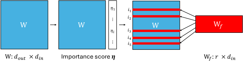
SPruFT utilizes structured neural network pruning to select a subset of the parameters for fine-tuning. NN pruning methods have been studied extensively (see Section 2) with the goal of reducing the size of a network (often fewer neurons) while preserving accuracy. These methods develop techniques for identifying neurons that are important for a given task. Our key insight is to use these importance metrics to indicate which neurons to focus on during fine-tuning. Note that, unlike pruning, where importance often reflects a neuron’s role in the original task, here it pertains to the downstream fine-tuning task, which may have a different input distribution and loss. In Section 4.2, we discuss various importance metrics from pruning research and discuss their use in fine-tuning.
Our method selects the top- important neurons based on an importance score , where is determined by the desired number of fine-tuning parameters. It follows that the choice of importance matric becomes crucial, which we discuss in Section 4.2. Let the top neuron indices be . After obtaining , we next construct a lower-dimensional parameter matrix , with the row selection matrix for all and zeros elsewhere. Using notations from Section 2, we initialize to zero and define the final parameters as Equation 1 where .
Let us now examine how to implement the forward to make backpropagation memory-efficient222While updating the corresponding rows of is the most efficient training, updating provides more flexibility for adapting multiple tasks, see discussion in LoRA (Hu et al., 2022).. If the computation graph were to pass through (as a naïve implementation would), the gradients would be computed for all parameters, which is redundant. Instead, we use the additivity of the forward function: we have, analogous to the setting of LoRA,
| (5) |
As remains frozen during fine-tuning, backpropagation only needs to keep track of the derivatives of the second term on the RHS. In addition, is now a fixed matrix, so the only trainable parameters are those in and will not be cached, while LoRA requires the cache of for computing (backpropagation, Rumelhart et al. 1986). Besides, as an SFT framework, our method does not rely on any dropout layer, which also saves a huge amount of memory. We explain this in detail in Appendix C.5 and we show that the benefits in terms of memory cost are significant in Section 6.1.
An important strength of our approach is its flexibility: it can easily incorporate any desired choice of importance metrics. On the other end, it can also incorporate new ideas in PEFT research. For example, quantization (QLoRA, Dettmers et al. 2024), parameter sharing (VeRA, Kopiczko et al. 2024), and combining SFT with LoRA (RoSA, Nikdan et al. 2024) can be used.
4.2 Importance Metrics
Importance evaluation plays a crucial role in our approach, as discussed above. We try various choices in our work: the first is the simple norm of the weight vector corresponding to each neuron; the second is the widely-used Taylor importance (LeCun et al., 1989). By considering the gradients, Taylor importance captures more information about the input distribution as well as the relevance of a neuron for the fine-tuning task of interest (which can be different from the original model). We also consider different variants of Taylor importance, as we discuss below. We remark that norm-based importance can be quite powerful on its own, as is the case with norm-sampling in the matrix approximation literature (Frieze et al., 2004).
4.2.1 Class Aware Taylor Importance
In our experiments on image classification tasks, we also consider a “class aware” variant of Taylor importance, which may be of independent interest. The motivation here comes from the observation that the importance of a neuron may depend on the class of an input example (as a toy example, a whisker-detecting neuron may be very important to the cat class, but not much to others; hence not too important on average). Another motivation comes from the observation that when we perform a vanilla (class agnostic) fine-tuning, the accuracy of some classes can be much worse than others — an undesirable outcome. This is shown in Table 2.
| #labels | Mean | Min | Q1 | Med | Q3 | Max | |
|---|---|---|---|---|---|---|---|
| CIFAR100 | 100 | 90.18 | 65 | 88 | 92 | 95 | 99 |
| Tiny-ImageNet | 200 | 87.55 | 62 | 84 | 88 | 92 | 100 |
We define the class-wise Taylor importance as follows: for neuron and label ,
| (6) |
where is the forward function of the entire model, denotes the average loss of over inputs in class , represents the forward without channel/neuron , and is the parameter vector of channel . One natural choice of importance of neuron motivated by the above discussion is . We find that this score is “too sensitive” (importance of neurons may be over-estimated because of just one class), leading to lower overall accuracy. On the other hand, the average (over ) of corresponds to the standard Taylor importance. We find that the intermediate quantity of Quantiles-Mean, defined as the average of the quantiles of the , works well in reducing the accuracy imbalance across labels, and also achieving a high overall accuracy. Formally,
| (7) |
where represents the -th quantile. See Appendix A for more details.
4.2.2 Zero-Order Taylor Importance
As discussed, Taylor importance can incorporate information about the data distribution and the fine-tuning task when evaluating important neurons. However, for large models like Llama-3, it turns out that the computational overhead required for computing Taylor importances is prohibitively large!333The Taylor importance here refers to computing the exact value without relying on approximations of the importance score or the gradient matrix used for deriving the importance score. In these cases, we apply the idea from the memory-efficient zeroth-order optimizer (MeZO, Malladi et al. 2023) to estimate the gradient in Taylor importance. The classical Zeroth-Order (ZO) setting is defined as below.
Definition 4.1 (Simultaneous Perturbation Stochastic Approximation or SPSA (Spall, 1992)).
Given a model with parameters and a loss function , SPSA estimates the gradient on a dataset as
where is drawn from , and is the scale of the perturbation. The -SPSA estimate averages over randomly sampled . Note that as , the estimate above converges to , which is equal to in expectation.
By applying SPSA, the Zero-Order Taylor (ZOTaylor) importance can be defined as follows:
| (8) |
where we denote and its estimate as and for convenience.
A naïve implementation of SPSA still requires twice the memory of inference because of the need to store . However, MeZO uses the trick of regenerating dynamically using a random seed (of much smaller size than the model), thus eliminating the storage and ensuring memory usage that is equal to that of inference. We now assess the effectiveness of ZOTaylor for our LLM.
Property 4.2.
-SPSA is an unbiased and consistent estimator with the variance where
Property 4.2 can be proved by simply noting that the covariance matrix of is , details can be found in Appendix A. With this property, we know that -SPSA can accurately estimate the gradient. However, the variance can be large when is large. Here, we first note that since we aim to find the most important neurons, we do not care about the gradient estimate itself. That is, given , our goal is to have a higher probability which is exactly equal to:
| (9) |
The lower bound of Equation 9 is and the probability will close to when the variance is large or when and are too close to one another. In our experiments, the values of from single SPSA lie in with variances ranging from to , thus the probability above turns out to be too close to .
To address this issue, we utilize a simple but highly effective strategy (J Reddi et al., 2015): we partition the training data into calibration sets. For each calibration set, we generate distinct perturbations to perform -SPSA, yielding gradient estimates. Consequently, the variance of -SPSA is effectively reduced to .444We note that this is not a formal guarantee; indeed, if is too large or the dataset is too small, there is additional variance across calibration sets that will become significant. In our experiments, we set and , where the variances fall within the range of , leading to a normalized value being approximately , which corresponds to the probability being close to .
Importantly, our objective is to select most of the top-% important neurons (for appropriate ), rather than ensuring the strict selection of all top-ranked neurons. Thus, the probability for any specific -pair does not need to be excessively high. A rigorous theoretical analysis of the optimal probability threshold is an interesting open direction. In this study, we primarily focus on demonstrating the feasibility of applying ZO-based approaches to importance metrics.
| Model, ft setting | mem | #param | ARC-c | ARC-e | BoolQ | HS | OBQA | PIQA | rte | SIQA | WG | Avg |
|---|---|---|---|---|---|---|---|---|---|---|---|---|
| Llama2(7B) | ||||||||||||
| LoRA, | 23.46GB | 159.9M(2.37%) | 44.97 | 77.02 | 77.43 | 57.75 | 32.0 | 78.45 | 62.09 | 47.75 | 68.75 | 60.69 |
| VeRA, | 22.97GB | 1.374M(0.02%) | 43.26 | 76.43 | 77.40 | 57.26 | 31.6 | 78.02 | 62.09 | 45.85 | 68.75 | 60.07 |
| DoRA, | 44.85GB | 161.3M(2.39%) | 44.71 | 77.02 | 77.55 | 57.79 | 32.4 | 78.29 | 61.73 | 47.90 | 68.98 | 60.71 |
| RoSA, | 44.69GB | 157.7M(2.34%) | 43.86 | 77.48 | 77.86 | 57.42 | 32.2 | 77.97 | 63.90 | 47.29 | 69.06 | 60.78 |
| SPruFT, | 17.62GB | 145.8M(2.16%) | 43.60 | 77.26 | 77.77 | 57.47 | 32.6 | 78.07 | 64.98 | 46.67 | 69.30 | 60.86 |
| Llama3(8B) | ||||||||||||
| LoRA, | 30.37GB | 167.8M(2.09%) | 53.07 | 81.40 | 82.32 | 60.67 | 34.2 | 79.98 | 69.68 | 48.52 | 73.56 | 64.82 |
| VeRA, | 29.49GB | 1.391M(0.02%) | 50.26 | 80.30 | 81.41 | 60.16 | 34.4 | 79.60 | 69.31 | 46.93 | 72.77 | 63.90 |
| DoRA, | 51.45GB | 169.1M(2.11%) | 53.33 | 81.57 | 82.45 | 60.71 | 34.2 | 80.09 | 69.31 | 48.67 | 73.64 | 64.88 |
| RoSA, | 48.40GB | 167.6M(2.09%) | 51.28 | 81.27 | 81.80 | 60.18 | 34.4 | 79.87 | 69.31 | 47.95 | 73.16 | 64.36 |
| SPruFT, | 24.49GB | 159.4M(1.98%) | 52.47 | 81.10 | 81.28 | 60.29 | 34.6 | 79.76 | 70.04 | 47.75 | 73.24 | 64.50 |
5 Experimental Setup
5.1 Datasets
We use multiple datasets for different tasks. For image classification, we fine-tune models on the training split and evaluate it on the validation split of Tiny-ImageNet (Tavanaei, 2020), CIFAR100 (Krizhevsky et al., 2009), and Caltech101 (Li et al., 2022). For text generation, we fine-tune LLMs on 256 samples from Stanford-Alpaca (Taori et al., 2023) and assess zero-shot performance on nine EleutherAI LM Harness tasks (Gao et al., 2021). See Appendix D for details.
5.2 Models and Baselines
We fine-tune full-precision Llama-2-7B and Llama-3-8B (float32) using our SPruFT, LoRA (Hu et al., 2022), VeRA (Kopiczko et al., 2024), DoRA (Liu et al., 2024), and RoSA (Nikdan et al., 2024). RoSA is chosen as the representative SFT method and is the only SFT due to the high memory demands of other SFT approaches, while full fine-tuning is excluded for the same reason. We freeze Llama’s classification layers and fine-tune only the linear layers in attention and MLP blocks.
Next, we evaluate importance metrics by fine-tuning Llamas and image models, including DeiT (Touvron et al., 2021), ViT (Dosovitskiy, 2020), ResNet101 (He et al., 2016), and ResNeXt101 (Xie et al., 2017) on CIFAR100, Caltech101, and Tiny-ImageNet. For image tasks, we set the fine-tuning ratio at 5%, meaning the trainable parameters are a total of 5% of the backbone plus classification layers.
5.3 Training Details
Our fine-tuning framework is built on torch-pruning555Torch-pruning is not required, all their implementations are based on PyTorch. (Fang et al., 2023), PyTorch (Paszke et al., 2019), PyTorch-Image-Models (Wightman, 2019), and HuggingFace Transformers (Wolf et al., 2020). Most experiments run on a single A100-80GB GPU, while DoRA and RoSA use an H100-96GB GPU. We use the Adam optimizer (Kingma & Ba, 2015) and fine-tune all models for a fixed number of epochs without validation-based model selection.
Image models: The learning rate is set to with cosine annealing decay (Loshchilov & Hutter, 2017), where the minimum learning rate is . All image models used in this study are pre-trained on ImageNet.
Llama: For LoRA and DoRA, we set , a dropout rate of , and a learning rate of with linear decay ( decay rate). For SPruFT, we control trainable parameters using rank instead of fine-tuning ratio for direct comparison. The learning rate is with the same decay settings. Linear decay is applied after a warmup over the first % of training steps. The maximum sequence length is , with truncation for longer inputs and padding for shorter ones.
6 Results and Discussion
We now present the results of fine-tuning image models and Llamas using our framework. We first apply our SPruFT to fine-tune Llama2 and Llama3 and compare the results with those obtained using LoRA and its variants. Following this, we examine the performance of our approach by utilizing various importance metrics.
6.1 Main Results of LLM
We apply our SPruFT method to fine-tune Llama2-7B and Llama3-8B, comparing the results with those obtained through LoRA and its variants. We select the magnitude of the neuron vector as the importance metric due to its low memory requirements, simplicity, and widely tested effectiveness. In contrast, gradient-based metrics like Taylor and Hessian are as memory-intensive as full LLM fine-tuning. While Wanda (Sun et al., 2024) offers a memory-efficient metric for pruning LLMs, it still requires one epoch of data forwarding and significantly more memory than inference to compute the input vector’s norm666We encountered an OOM error when using Wanda’s official implementation. When pruning a neural network, each layer computes Wanda and is pruned immediately, gradually reducing the model size. However, in the fine-tuning process, the model size remains unchanged. Additionally, storing the norm values for computing importance scores further increases memory consumption, making memory cost significantly higher than when using Wanda for pruning.. For epochs choosing, we opt for 5 epochs to balance computational resources and performance.
Table 3 demonstrates the exceptional memory efficiency of our approach777Also refer to Table 12 in Appendix C.6, even with , our method’s memory usage remains significantly lower than that of LoRA with . while achieving comparable accuracy. As shown, the accuracies of fine-tuned models remain similar across most PEFT methods, while memory usage varies significantly. VeRA, despite having significantly fewer trainable parameters, shows noticeably lower accuracy. Notably, our approach consistently requires substantially less memory than all other PEFT methods listed in the table.
| Model, ft setting | mem | #param | Avg |
|---|---|---|---|
| Llama2(7B), LoRA, | 21.64GB | 40.0M(0.59%) | 60.55 |
| Llama2(7B), FA-LoRA, | 16.56GB | 46.4M(0.69%) | 60.71 |
| Llama2(7B), LoRA, | 22.21GB | 80.0M(1.19%) | 60.92 |
| Llama2(7B), FA-LoRA, | 17.25GB | 92.8M(1.38%) | 60.85 |
| Llama2(7B), SPruFT, | 15.57GB | 36.4M(0.54%) | 60.52 |
| Llama2(7B), FA-SPruFT, | 14.48GB | 39.3M(0.58%) | 60.82 |
| Llama2(7B), SPruFT, | 16.20GB | 72.9M(1.08%) | 60.67 |
| Llama2(7B), FA-SPruFT, | 15.21GB | 78.6M(1.17%) | 60.87 |
| Llama3(8B), LoRA, | 28.86GB | 41.9M(0.52%) | 64.76 |
| Llama3(8B), FA-LoRA, | 23.89GB | 56.6M(0.71%) | 64.81 |
| Llama3(8B), LoRA, | 29.37GB | 83.9M(1.04%) | 64.76 |
| Llama3(8B), FA-LoRA, | 24.55GB | 113.2M(1.41%) | 64.77 |
| Llama3(8B), SPruFT, | 22.62GB | 39.8M(0.50%) | 64.21 |
| Llama3(8B), FA-SPruFT, | 21.62GB | 46.1M(0.57%) | 64.56 |
| Llama3(8B), SPruFT, | 23.23GB | 79.7M(0.99%) | 64.51 |
| Llama3(8B), FA-SPruFT, | 22.41GB | 92.3M(1.15%) | 64.26 |
We then demonstrate that strategically assigning trainable parameters saves more memory than merely reducing them, without compromising accuracy. We compare fine-tuning all linear layers and fine-tuning only the MLP layers, with results shown in Table 4. The former requires more memory for the same number of trainable parameters, as distributing trainable parameters across the model increases the need for caching intermediate values. Recalling the results from Table 1 in Section 3, freezing attention blocks provides significantly greater memory savings than reducing LoRA’s trainable parameters. Additionally, accuracy remains nearly unchanged. Given that Llama models have been pre-trained on extensive datasets, their attention blocks likely already capture crucial patterns for token interactions. Our results suggest that freezing these attention blocks maintains performance nearly equivalent to fine-tuning all layers.
6.2 Importance Metrics
| model | imp | CIFAR100 | Tiny-ImageNet | Caltech101 |
|---|---|---|---|---|
| DeiT | FFT | 90.18 | 87.55 | 97.33 |
| 88.05 | 89.31 | 95.01 | ||
| Taylor | 88.70 | 89.69 | 95.41 | |
| QMTaylor | 89.37 | 89.75 | - | |
| ViT | FFT | 90.13 | 88.45 | 97.16 |
| 87.13 | 90.78 | 92.69 | ||
| Taylor | 88.06 | 90.87 | 93.96 | |
| QMTaylor | 88.51 | 90.90 | - | |
| RN | FFT | 86.21 | 77.78 | 96.50 |
| 82.25 | 79.83 | 93.13 | ||
| Taylor | 82.36 | 79.66 | 92.56 | |
| QMTaylor | 83.50 | 80.02 | - | |
| RNX | FFT | 87.30 | 79.51 | 97.07 |
| 86.12 | 83.88 | 95.71 | ||
| Taylor | 85.94 | 83.88 | 95.84 | |
| QMTaylor | 86.93 | 84.17 | - |
| Settings | Avg | |
|---|---|---|
| Llama2(7B) | Llama3(8B) | |
| , random | 60.25 | 64.00 |
| , | 60.86 | 64.50 |
| , ZOTaylor | 60.94 | 64.67 |
| , FA, random | 60.35 | 63.95 |
| , FA, | 60.87 | 64.26 |
| , FA, ZOTaylor | 60.87 | 64.38 |
We apply various importance metrics to fine-tune Llamas and image models using our approach and report the results to compare their performance. As shown in Table 5 and Table 6, Quantile-Mean Taylor and ZOTaylor offer slight improvements over other importance metrics. For image tasks, while the differences among importance metrics are not substantial, the results consistently indicate that Quantile-Mean Taylor slightly outperforms standard Taylor importance. Additionally, both Quantile-Mean Taylor and standard Taylor importance outperform magnitude-based importance.
Similarly, in the cases of Llama2 and Llama3, our findings suggest that ZOTaylor provides a slight performance boost for fine-tuned models. This improvement is likely due to ZOTaylor’s ability to capture richer data information, whereas magnitude-based importance tends to focus more on identifying generally important neurons. However, the observed performance gain remains modest, potentially due to the variance of the estimates, as discussed in Section 4.2.2. Beyond these observations, another interesting finding is that fine-tuned models with random row selection perform similarly to VeRA, likely suggesting that this accuracy level could serve as a baseline for other fine-tuning approaches.
7 Conclusions and Future Work
We propose a parameter-efficient fine-tuning (PEFT) framework that integrates various techniques and importance metrics from model compression research to enhance sparse fine-tuning (SFT). Using our method, we can fine-tune LLMs and vision transformers using significantly less computation resources than the popular LoRA (Low-Rank Adaptation) technique, while achieving similar accuracy. We also explore the effects of using different importance metrics. There are several future directions: (1) For importance metrics, while Quantile-Mean Taylor shows slight improvements, these gains are relatively minor compared to the standard Taylor metric in some cases of DeiT and ViT. We may wish to explore better metrics for classification tasks with a large number of labels. (2) Developing memory-efficient importance metrics for LLMs is another future direction. While Zeroth-Order Taylor is effective for incorporating data-specific information without requiring large memory, the large variance of estimate is a challenge. Although we reduce the variance effectively by increasing the number of estimations, exploring a simple method to reduce variance without increasing estimation times is essential for further advancements in this field. (3) Our results show that fine-tuning a small number of neurons can significantly improve model performance on downstream tasks. This observation naturally raises the question: do the selected neurons play a distinctive role in specific tasks? This question is related to the explainability of neural networks, which is an extensive area of research. It will be interesting to understand if (and how) individual neurons chosen for fine-tuning contribute to the new task.
References
- Achiam et al. (2023) Achiam, J., Adler, S., Agarwal, S., Ahmad, L., Akkaya, I., Aleman, F. L., Almeida, D., Altenschmidt, J., Altman, S., Anadkat, S., et al. Gpt-4 technical report. arXiv preprint arXiv:2303.08774, 2023.
- Ansell et al. (2022) Ansell, A., Ponti, E., Korhonen, A., and Vulić, I. Composable sparse fine-tuning for cross-lingual transfer. In Proceedings of the 60th Annual Meeting of the Association for Computational Linguistics (Volume 1: Long Papers), pp. 1778–1796, 2022.
- Bar-Haim et al. (2006) Bar-Haim, R., Dagan, I., Dolan, B., Ferro, L., Giampiccolo, D., Magnini, B., and Szpektor, I. The second PASCAL recognising textual entailment challenge. 2006.
- Bentivogli et al. (2009) Bentivogli, L., Dagan, I., Dang, H. T., Giampiccolo, D., and Magnini, B. The fifth PASCAL recognizing textual entailment challenge. 2009.
- Bienaymé (1853) Bienaymé, I.-J. Considérations à l’appui de la découverte de Laplace sur la loi de probabilité dans la méthode des moindres carrés. Imprimerie de Mallet-Bachelier, 1853.
- Bisk et al. (2020) Bisk, Y., Zellers, R., Bras, R. L., Gao, J., and Choi, Y. Piqa: Reasoning about physical commonsense in natural language. In Thirty-Fourth AAAI Conference on Artificial Intelligence, 2020.
- Cer et al. (2017) Cer, D., Diab, M., Agirre, E., Lopez-Gazpio, I., and Specia, L. SemEval-2017 task 1: Semantic textual similarity multilingual and crosslingual focused evaluation. In Bethard, S., Carpuat, M., Apidianaki, M., Mohammad, S. M., Cer, D., and Jurgens, D. (eds.), Proceedings of the 11th International Workshop on Semantic Evaluation (SemEval-2017), pp. 1–14, Vancouver, Canada, August 2017. Association for Computational Linguistics. doi: 10.18653/v1/S17-2001. URL https://aclanthology.org/S17-2001.
- Clark et al. (2019) Clark, C., Lee, K., Chang, M.-W., Kwiatkowski, T., Collins, M., and Toutanova, K. Boolq: Exploring the surprising difficulty of natural yes/no questions. In Proceedings of the 2019 Conference of the North American Chapter of the Association for Computational Linguistics: Human Language Technologies, Volume 1 (Long and Short Papers), pp. 2924–2936, 2019.
- Clark et al. (2018) Clark, P., Cowhey, I., Etzioni, O., Khot, T., Sabharwal, A., Schoenick, C., and Tafjord, O. Think you have solved question answering? try arc, the ai2 reasoning challenge. arXiv preprint arXiv:1803.05457, 2018.
- Dagan et al. (2006) Dagan, I., Glickman, O., and Magnini, B. The PASCAL recognising textual entailment challenge. In Machine learning challenges. evaluating predictive uncertainty, visual object classification, and recognising tectual entailment, pp. 177–190. Springer, 2006.
- Deng et al. (2009) Deng, J., Dong, W., Socher, R., Li, L.-J., Li, K., and Fei-Fei, L. Imagenet: A large-scale hierarchical image database. In 2009 IEEE conference on computer vision and pattern recognition, pp. 248–255. Ieee, 2009.
- Dettmers et al. (2022) Dettmers, T., Lewis, M., Belkada, Y., and Zettlemoyer, L. Gpt3. int8 (): 8-bit matrix multiplication for transformers at scale. Advances in Neural Information Processing Systems, 35:30318–30332, 2022.
- Dettmers et al. (2024) Dettmers, T., Pagnoni, A., Holtzman, A., and Zettlemoyer, L. Qlora: Efficient finetuning of quantized llms. Advances in Neural Information Processing Systems, 36, 2024.
- Dolan & Brockett (2005) Dolan, W. B. and Brockett, C. Automatically constructing a corpus of sentential paraphrases. In Proceedings of the International Workshop on Paraphrasing, 2005.
- Dosovitskiy (2020) Dosovitskiy, A. An image is worth 16x16 words: Transformers for image recognition at scale. arXiv preprint arXiv:2010.11929, 2020.
- Dubey et al. (2024) Dubey, A., Jauhri, A., Pandey, A., Kadian, A., Al-Dahle, A., Letman, A., Mathur, A., Schelten, A., Yang, A., Fan, A., et al. The llama 3 herd of models. arXiv preprint arXiv:2407.21783, 2024.
- Fang et al. (2023) Fang, G., Ma, X., Song, M., Mi, M. B., and Wang, X. Depgraph: Towards any structural pruning. In Proceedings of the IEEE/CVF conference on computer vision and pattern recognition, pp. 16091–16101, 2023.
- Frantar & Alistarh (2023) Frantar, E. and Alistarh, D. Sparsegpt: Massive language models can be accurately pruned in one-shot. In International Conference on Machine Learning, pp. 10323–10337. PMLR, 2023.
- Frieze et al. (2004) Frieze, A., Kannan, R., and Vempala, S. Fast monte-carlo algorithms for finding low-rank approximations. J. ACM, 51(6):1025–1041, November 2004. ISSN 0004-5411. doi: 10.1145/1039488.1039494. URL https://doi.org/10.1145/1039488.1039494.
- Gale et al. (2020) Gale, T., Zaharia, M., Young, C., and Elsen, E. Sparse gpu kernels for deep learning. In SC20: International Conference for High Performance Computing, Networking, Storage and Analysis, pp. 1–14. IEEE, 2020.
- Gao et al. (2021) Gao, L., Tow, J., Biderman, S., Black, S., DiPofi, A., Foster, C., Golding, L., Hsu, J., McDonell, K., Muennighoff, N., et al. A framework for few-shot language model evaluation. Version v0. 0.1. Sept, 10:8–9, 2021.
- Gholami et al. (2022) Gholami, A., Kim, S., Dong, Z., Yao, Z., Mahoney, M. W., and Keutzer, K. A survey of quantization methods for efficient neural network inference. In Low-Power Computer Vision, pp. 291–326. Chapman and Hall/CRC, 2022.
- Giampiccolo et al. (2007) Giampiccolo, D., Magnini, B., Dagan, I., and Dolan, B. The third PASCAL recognizing textual entailment challenge. In Proceedings of the ACL-PASCAL workshop on textual entailment and paraphrasing, pp. 1–9. Association for Computational Linguistics, 2007.
- Guo et al. (2021) Guo, D., Rush, A., and Kim, Y. Parameter-efficient transfer learning with diff pruning. In Annual Meeting of the Association for Computational Linguistics, 2021.
- Guo et al. (2024a) Guo, H., Greengard, P., Xing, E., and Kim, Y. LQ-loRA: Low-rank plus quantized matrix decomposition for efficient language model finetuning. In The Twelfth International Conference on Learning Representations, 2024a. URL https://openreview.net/forum?id=xw29VvOMmU.
- Guo et al. (2024b) Guo, W., Long, J., Zeng, Y., Liu, Z., Yang, X., Ran, Y., Gardner, J. R., Bastani, O., De Sa, C., Yu, X., et al. Zeroth-order fine-tuning of llms with extreme sparsity. arXiv preprint arXiv:2406.02913, 2024b.
- Han (2017) Han, S. Efficient methods and hardware for deep learning. PhD thesis, Stanford University, 2017.
- Han et al. (2015) Han, S., Pool, J., Tran, J., and Dally, W. Learning both weights and connections for efficient neural network. Advances in neural information processing systems, 28, 2015.
- He et al. (2016) He, K., Zhang, X., Ren, S., and Sun, J. Deep residual learning for image recognition. In Proceedings of the IEEE conference on computer vision and pattern recognition, pp. 770–778, 2016.
- He et al. (2023) He, P., Gao, J., and Chen, W. Debertav3: Improving deberta using electra-style pre-training with gradient-disentangled embedding sharing. In The Eleventh International Conference on Learning Representations, 2023.
- Hoefler et al. (2021) Hoefler, T., Alistarh, D., Ben-Nun, T., Dryden, N., and Peste, A. Sparsity in deep learning: Pruning and growth for efficient inference and training in neural networks. Journal of Machine Learning Research, 22(241):1–124, 2021.
- Holmes et al. (2021) Holmes, C., Zhang, M., He, Y., and Wu, B. Nxmtransformer: semi-structured sparsification for natural language understanding via admm. Advances in neural information processing systems, 34:1818–1830, 2021.
- Hu et al. (2022) Hu, E. J., Wallis, P., Allen-Zhu, Z., Li, Y., Wang, S., Wang, L., Chen, W., et al. Lora: Low-rank adaptation of large language models. In International Conference on Learning Representations, 2022.
- J Reddi et al. (2015) J Reddi, S., Hefny, A., Sra, S., Poczos, B., and Smola, A. J. On variance reduction in stochastic gradient descent and its asynchronous variants. Advances in neural information processing systems, 28, 2015.
- Jiang et al. (2022) Jiang, P., Hu, L., and Song, S. Exposing and exploiting fine-grained block structures for fast and accurate sparse training. Advances in Neural Information Processing Systems, 35:38345–38357, 2022.
- Kingma & Ba (2015) Kingma, D. and Ba, J. Adam: A method for stochastic optimization. International Conference on Learning Representations (ICLR), 2015.
- Kopiczko et al. (2024) Kopiczko, D. J., Blankevoort, T., and Asano, Y. M. VeRA: Vector-based random matrix adaptation. In The Twelfth International Conference on Learning Representations, 2024. URL https://openreview.net/forum?id=NjNfLdxr3A.
- Krizhevsky et al. (2009) Krizhevsky, A. et al. Learning multiple layers of features from tiny images. 2009.
- LeCun et al. (1989) LeCun, Y., Denker, J., and Solla, S. Optimal brain damage. Advances in neural information processing systems, 2, 1989.
- Li et al. (2022) Li, F.-F., Andreeto, M., Ranzato, M., and Perona, P. Caltech 101, Apr 2022.
- Li et al. (2024) Li, Y., Yu, Y., Liang, C., Karampatziakis, N., He, P., Chen, W., and Zhao, T. Loftq: LoRA-fine-tuning-aware quantization for large language models. In The Twelfth International Conference on Learning Representations, 2024. URL https://openreview.net/forum?id=LzPWWPAdY4.
- Lialin et al. (2023) Lialin, V., Deshpande, V., and Rumshisky, A. Scaling down to scale up: A guide to parameter-efficient fine-tuning. arXiv preprint arXiv:2303.15647, 2023.
- Liu et al. (2021) Liu, L., Zhang, S., Kuang, Z., Zhou, A., Xue, J.-H., Wang, X., Chen, Y., Yang, W., Liao, Q., and Zhang, W. Group fisher pruning for practical network compression. In International Conference on Machine Learning, pp. 7021–7032. PMLR, 2021.
- Liu et al. (2024) Liu, S.-Y., Wang, C.-Y., Yin, H., Molchanov, P., Wang, Y.-C. F., Cheng, K.-T., and Chen, M.-H. DoRA: Weight-decomposed low-rank adaptation. In Forty-first International Conference on Machine Learning, 2024. URL https://openreview.net/forum?id=3d5CIRG1n2.
- Loshchilov & Hutter (2017) Loshchilov, I. and Hutter, F. Sgdr: Stochastic gradient descent with warm restarts. In International Conference on Learning Representations, 2017.
- Lu et al. (2024) Lu, X., Zhou, A., Xu, Y., Zhang, R., Gao, P., and Li, H. SPP: Sparsity-preserved parameter-efficient fine-tuning for large language models. In Forty-first International Conference on Machine Learning, 2024. URL https://openreview.net/forum?id=9Rroj9GIOQ.
- Ma et al. (2023) Ma, X., Fang, G., and Wang, X. LLM-pruner: On the structural pruning of large language models. In Thirty-seventh Conference on Neural Information Processing Systems, 2023. URL https://openreview.net/forum?id=J8Ajf9WfXP.
- Malladi et al. (2023) Malladi, S., Gao, T., Nichani, E., Damian, A., Lee, J. D., Chen, D., and Arora, S. Fine-tuning language models with just forward passes. Advances in Neural Information Processing Systems, 36:53038–53075, 2023.
- Micikevicius et al. (2018) Micikevicius, P., Narang, S., Alben, J., Diamos, G., Elsen, E., Garcia, D., Ginsburg, B., Houston, M., Kuchaiev, O., Venkatesh, G., and Wu, H. Mixed precision training. In International Conference on Learning Representations, 2018. URL https://openreview.net/forum?id=r1gs9JgRZ.
- Mihaylov et al. (2018) Mihaylov, T., Clark, P., Khot, T., and Sabharwal, A. Can a suit of armor conduct electricity? a new dataset for open book question answering. In Proceedings of the 2018 Conference on Empirical Methods in Natural Language Processing, pp. 2381–2391, 2018.
- Mofrad et al. (2019) Mofrad, M. H., Melhem, R., Ahmad, Y., and Hammoud, M. Multithreaded layer-wise training of sparse deep neural networks using compressed sparse column. In 2019 IEEE High Performance Extreme Computing Conference (HPEC), pp. 1–6. IEEE, 2019.
- Nikdan et al. (2023) Nikdan, M., Pegolotti, T., Iofinova, E., Kurtic, E., and Alistarh, D. SparseProp: Efficient sparse backpropagation for faster training of neural networks at the edge. In Krause, A., Brunskill, E., Cho, K., Engelhardt, B., Sabato, S., and Scarlett, J. (eds.), Proceedings of the 40th International Conference on Machine Learning, volume 202 of Proceedings of Machine Learning Research, pp. 26215–26227. PMLR, 23–29 Jul 2023. URL https://proceedings.mlr.press/v202/nikdan23a.html.
- Nikdan et al. (2024) Nikdan, M., Tabesh, S., Crnčević, E., and Alistarh, D. RoSA: Accurate parameter-efficient fine-tuning via robust adaptation. In Forty-first International Conference on Machine Learning, 2024. URL https://openreview.net/forum?id=FYvpxyS43U.
- Panigrahi et al. (2023) Panigrahi, A., Saunshi, N., Zhao, H., and Arora, S. Task-specific skill localization in fine-tuned language models. In International Conference on Machine Learning, pp. 27011–27033. PMLR, 2023.
- Paszke et al. (2019) Paszke, A., Gross, S., Massa, F., Lerer, A., Bradbury, J., Chanan, G., Killeen, T., Lin, Z., Gimelshein, N., Antiga, L., et al. Pytorch: An imperative style, high-performance deep learning library. Advances in neural information processing systems, 32, 2019.
- Peste et al. (2021) Peste, A., Iofinova, E., Vladu, A., and Alistarh, D. Ac/dc: Alternating compressed/decompressed training of deep neural networks. Advances in neural information processing systems, 34:8557–8570, 2021.
- Rajpurkar et al. (2016) Rajpurkar, P., Zhang, J., Lopyrev, K., and Liang, P. SQuAD: 100,000+ questions for machine comprehension of text. In Proceedings of EMNLP, pp. 2383–2392. Association for Computational Linguistics, 2016.
- Rissanen (1996) Rissanen, J. J. Fisher information and stochastic complexity. IEEE transactions on information theory, 42(1):40–47, 1996.
- Rumelhart et al. (1986) Rumelhart, D. E., Hinton, G. E., and Williams, R. J. Learning representations by back-propagating errors. nature, 323(6088):533–536, 1986.
- Sakaguchi et al. (2021) Sakaguchi, K., Bras, R. L., Bhagavatula, C., and Choi, Y. Winogrande: An adversarial winograd schema challenge at scale. Communications of the ACM, 64(9):99–106, 2021.
- Sap et al. (2019) Sap, M., Rashkin, H., Chen, D., Le Bras, R., and Choi, Y. Social IQa: Commonsense reasoning about social interactions. In Inui, K., Jiang, J., Ng, V., and Wan, X. (eds.), Proceedings of the 2019 Conference on Empirical Methods in Natural Language Processing and the 9th International Joint Conference on Natural Language Processing (EMNLP-IJCNLP), pp. 4463–4473, Hong Kong, China, November 2019. Association for Computational Linguistics. doi: 10.18653/v1/D19-1454. URL https://aclanthology.org/D19-1454/.
- Schwarz et al. (2021) Schwarz, J., Jayakumar, S., Pascanu, R., Latham, P. E., and Teh, Y. Powerpropagation: A sparsity inducing weight reparameterisation. Advances in neural information processing systems, 34:28889–28903, 2021.
- Socher et al. (2013) Socher, R., Perelygin, A., Wu, J., Chuang, J., Manning, C. D., Ng, A., and Potts, C. Recursive deep models for semantic compositionality over a sentiment treebank. In Proceedings of EMNLP, pp. 1631–1642, 2013.
- Spall (1992) Spall, J. C. Multivariate stochastic approximation using a simultaneous perturbation gradient approximation. IEEE transactions on automatic control, 37(3):332–341, 1992.
- Sun et al. (2024) Sun, M., Liu, Z., Bair, A., and Kolter, J. Z. A simple and effective pruning approach for large language models. In The Twelfth International Conference on Learning Representations, 2024.
- Sung et al. (2021) Sung, Y.-L., Nair, V., and Raffel, C. A. Training neural networks with fixed sparse masks. Advances in Neural Information Processing Systems, 34:24193–24205, 2021.
- Taori et al. (2023) Taori, R., Gulrajani, I., Zhang, T., Dubois, Y., Li, X., Guestrin, C., Liang, P., and Hashimoto, T. B. Stanford alpaca: An instruction-following llama model. https://github.com/tatsu-lab/stanford_alpaca, 2023.
- Tavanaei (2020) Tavanaei, A. Embedded encoder-decoder in convolutional networks towards explainable ai. arXiv preprint arXiv:2007.06712, 2020.
- Tchébychef (1867) Tchébychef, P. Des valeurs moyennes, volume 12. Journal de Mathématiques Pures et Appliquées 2, 1867.
- Touvron et al. (2021) Touvron, H., Cord, M., Douze, M., Massa, F., Sablayrolles, A., and Jégou, H. Training data-efficient image transformers & distillation through attention. In International conference on machine learning, pp. 10347–10357. PMLR, 2021.
- Vaswani (2017) Vaswani, A. Attention is all you need. Advances in Neural Information Processing Systems, 2017.
- Warstadt et al. (2018) Warstadt, A., Singh, A., and Bowman, S. R. Neural network acceptability judgments. arXiv preprint 1805.12471, 2018.
- Wightman (2019) Wightman, R. Pytorch image models. https://github.com/rwightman/pytorch-image-models, 2019.
- Williams et al. (2018) Williams, A., Nangia, N., and Bowman, S. R. A broad-coverage challenge corpus for sentence understanding through inference. In Proceedings of NAACL-HLT, 2018.
- Wolf et al. (2020) Wolf, T., Debut, L., Sanh, V., Chaumond, J., Delangue, C., Moi, A., Cistac, P., Rault, T., Louf, R., Funtowicz, M., et al. Transformers: State-of-the-art natural language processing. In Proceedings of the 2020 conference on empirical methods in natural language processing: system demonstrations, pp. 38–45, 2020.
- Xie et al. (2017) Xie, S., Girshick, R., Dollár, P., Tu, Z., and He, K. Aggregated residual transformations for deep neural networks. In Proceedings of the IEEE conference on computer vision and pattern recognition, pp. 1492–1500, 2017.
- Xu et al. (2024) Xu, M., Yin, W., Cai, D., Yi, R., Xu, D., Wang, Q., Wu, B., Zhao, Y., Yang, C., Wang, S., et al. A survey of resource-efficient llm and multimodal foundation models. arXiv preprint arXiv:2401.08092, 2024.
- Zellers et al. (2019) Zellers, R., Holtzman, A., Bisk, Y., Farhadi, A., and Choi, Y. Hellaswag: Can a machine really finish your sentence? In Proceedings of the 57th Annual Meeting of the Association for Computational Linguistics. Association for Computational Linguistics, 2019.
- Zhang et al. (2020) Zhang, Z., Wang, H., Han, S., and Dally, W. J. Sparch: Efficient architecture for sparse matrix multiplication. In 2020 IEEE International Symposium on High Performance Computer Architecture (HPCA), pp. 261–274. IEEE, 2020.
- Zhou et al. (2024) Zhou, A., Wang, K., Lu, Z., Shi, W., Luo, S., Qin, Z., Lu, S., Jia, A., Song, L., Zhan, M., et al. Solving challenging math word problems using gpt-4 code interpreter with code-based self-verification. In The Twelfth International Conference on Learning Representations, 2024.
Appendix A Importance Metrics
Taylor importance is the Taylor expansion of the difference between the loss of the model with and without the target neuron:
where . (**) is from the result of Fisher information (Rissanen, 1996):
Note that (*) is from , as removing one channel/neuron from a large neural network typically results in only a negligible reduction in loss. To efficiently compute , the equation can be further derived as:
where .
Magnitude importance is the -norm of the neuron vector computed as .
Proof of Property 4.2
To prove Property 4.2, we first calculate the expectation and variance of SPSA. For convenience, we denote as . Then, the expectation is as follows:
The variance can then be derived as follows:
, , and are because . is obtained from the moment generating function of standard normal:
Thus, the expectation and variance of -SPSA estimate are
Appendix B Parameter Dependency
Dependencies of parameters between neurons or channels across different layers exist in NNs. These include basic layer connections, residual connections, tensor concatenations, summations, and more, as shown in Figure 2. The black neurons connected by real lines represent the dependent parameters that are in the same group. Pruning any black neurons results in removing the parameters connected by the real lines. (Liu et al., 2021) introduced a group pruning method for CNN models that treats residual connections as grouped dependencies, evaluating and pruning related channels within the same group simultaneously. Similarly, (Fang et al., 2023) proposed a novel group pruning technique named Torch-Pruning, which considers various types of dependencies and achieves state-of-the-art results. (Ma et al., 2023) further applied this procedure to pruning LLMs. Torch-Pruning can be applied to prune a wide range of neural networks, including image transformers, LLMs, CNNs, and more, making it a popular toolkit for neural network pruning.
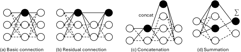
In this study, we also evaluate the influences of incorporating parameter dependency in our approach. We put the experimental results of whether incorporating parameter dependency in Appendix C.2. In the experiments, parameter dependency becomes the following process for our approach: first, searching for dependencies by tracing the computation graph of gradient; next, evaluating the importance of parameter groups; and finally, fine-tuning the parameters within those important groups collectively. For instance, if and are dependent, where is the -th column in parameter matrix (or the -th input channels/features) of layer and is the -th row in parameter matrix (or the -th output channels/features) of layer , then and will be fine-tuned simultaneously while the corresponding for becomes column selection matrix and becomes . Consequently, fine-tuning output channels for layer will result in fine-tuning additional input channels in each dependent layer. Therefore, for the of desired fine-tuning ratio, the fine-tuning ratio with considering dependencies is set to 888In some complex models, considering dependencies results in slightly more than twice the number of trainable parameters. However, in most cases, the factor is 2. for the approach that includes dependencies.
The forward function of layer for column selection mentioned above can be written as the following equation:
Note that in this example, as the dependency is connection between the output feature/channel of and the input feature/channel of , the dimension is equal to where .
Appendix C Ablation Studies and Related Analysis
In this section, we first discuss the hyperparameter settings. While we do not include DeBERTaV3 (He et al., 2023) in the main context, we fine-tune DeBERTaV3-base (He et al., 2023) on GLUE. The learning rate is set to with linear decay, where the decay rate is . The model is fine-tuned on the full training split of 8 tasks from the GLUE benchmark. The maximum sequence length is fixed to 256 with longer sequences truncated and shorter sequences padded. Note that memory efficiency is not emphasized for small-scale models, as dataset-related memory—particularly with large batch sizes—dominates consumption in these cases. The main advantage of our method in these cases is the reduced FLOPs due to fewer trainable parameters.
Following this, we discuss the computational resource requirements for fine-tuning. Figure 4 illustrates the computation and cache requirements during backpropagation. Next, we provide an ablation study on the impact of different rank settings for our approach and LoRA, as shown in Table 12. Finally, Table 14 demonstrates the advantages of freezing self-attention blocks to reduce memory usage while maintaining performance.
| CIFAR100 | Tiny-ImageNet | Caltech101 | |||||||
| Full | Head | SPruFT | Full | Head | SPruFT | Full | Head | SPruFT | |
| #ep | loss, acc | loss, acc | loss, acc | loss, acc | loss, acc | loss, acc | loss, acc | loss, acc | loss, acc |
| DeiT | DeiT | DeiT | |||||||
| #param: | 86.0M | 0.2M | 4.6M | 86.1M | 0.3M | 4.8M | 86.0M | 0.2M | 4.6M |
| 5 | 0.36, 90.18 | 0.76, 80.25 | 0.37, 88.70 | 0.54, 87.55 | 0.60, 85.09 | 0.40, 89.69 | 0.11, 97.33 | 1.09, 89.02 | 0.30, 95.41 |
| 10 | 0.44, 90.04 | 0.64, 81.83 | 0.42, 88.62 | 0.69, 86.32 | 0.54, 85.72 | 0.49, 88.96 | 0.11, 97.55 | 0.53, 93.22 | 0.17, 96.28 |
| 30 | 0.62, 89.03 | 0.55, 83.42 | 0.64, 88.61 | 0.94, 84.27 | 0.52, 86.06 | 0.72, 88.67 | 0.11, 97.11 | 0.22, 95.06 | 0.12, 96.50 |
| ViT | ViT | ViT | |||||||
| #param: | 85.9M | 0.1M | 4.5M | 86.0M | 0.2M | 4.6M | 85.9M | 0.1M | 45.2M |
| 5 | 0.38, 90.13 | 1.01, 74.78 | 0.40, 88.13 | 0.51, 88.45 | 0.65, 84.10 | 0.36, 90.87 | 0.12, 97.16 | 1.60, 85.70 | 0.43, 93.96 |
| 10 | 0.45, 89.85 | 0.85, 77.05 | 0.45, 87.55 | 0.66, 86.78 | 0.58, 84.95 | 0.44, 90.48 | 0.11, 97.20 | 0.85, 89.98 | 0.23, 95.54 |
| 30 | 0.62, 88.78 | 0.71, 79.51 | 0.69, 87.83 | 0.96, 84.20 | 0.55, 85.49 | 0.61, 90.56 | 0.12, 97.24 | 0.33, 92.65 | 0.16, 96.02 |
| ResNet101 | ResNet101 | ResNet101 | |||||||
| #param: | 42.7M | 0.2M | 2.2M | 42.9M | 0.4M | 2.4M | 42.7M | 0.2M | 2.2M |
| 5 | 0.50, 86.21 | 1.62, 60.78 | 0.59, 82.36 | 0.92, 77.78 | 1.64, 62.06 | 0.76, 79.66 | 0.14, 96.50 | 1.25, 82.33 | 0.48, 92.56 |
| 10 | 0.58, 86.41 | 1.39, 63.06 | 0.60, 82.33 | 1.10, 76.81 | 1.50, 63.19 | 0.79, 79.54 | 0.14, 96.54 | 0.69, 90.24 | 0.23, 95.58 |
| 30 | 0.80, 84.72 | 1.21, 65.63 | 0.80, 82.49 | 1.54, 74.09 | 1.43, 64.47 | 1.08, 78.58 | 0.18, 95.80 | 0.31, 93.00 | 0.16, 95.89 |
| ResNeXt101 | ResNeXt101 | ResNeXt101 | |||||||
| #param: | 87.0M | 0.2M | 4.9M | 87.2M | 0.4M | 5.1M | 87.0M | 0.2M | 4.9M |
| 5 | 0.47, 87.30 | 1.42, 65.07 | 0.47, 85.94 | 0.86, 79.51 | 1.46, 65.59 | 0.61, 83.88 | 0.12, 97.07 | 1.25, 83.16 | 0.28, 95.84 |
| 10 | 0.56, 87.17 | 1.23, 67.55 | 0.53, 86.04 | 1.01, 79.27 | 1.35, 66.73 | 0.69, 83.47 | 0.13, 96.89 | 0.68, 90.94 | 0.18, 96.28 |
| 30 | 0.71, 86.59 | 1.08, 69.45 | 0.69, 86.33 | 1.41, 76.55 | 1.29, 67.93 | 0.90, 82.83 | 0.16, 96.63 | 0.31, 92.87 | 0.14, 96.76 |
C.1 Hyperparameter Settings
We report the results of three approaches over several epochs as table 7 and table 8. Overall, full fine-tuning over higher epochs is more prone to overfitting, while head fine-tuning shows the exact opposite trend. Except for the results on caltech101999The inconsistent trend observed in Caltech101 results is likely due to its significantly smaller sample size., the loss patterns across all models consistently reflect this trend, and most accuracy results further support this conclusion. However, our approach demonstrates a crucial advantage by effectively balancing the tradeoff between performance and computational resources.
Table 7 clearly shows that both our approach and full fine-tuning achieve optimal results within a few epochs, while head fine-tuning requires more training. Notably, all models have been pre-trained on ImageNet-1k, which may explain the strong performance observed with head fine-tuning on Tiny-ImageNet. However, even with this advantage, full fine-tuning still outperforms head fine-tuning, and our approach surpasses both. In just 5 epochs, our approach achieves results comparable to full fine-tuning on all datasets with significantly lower trainable parameters.
| task | CoLA | MNLI | MRPC | QNLI | QQP | RTE | SST-2 | STS-B | ||
|---|---|---|---|---|---|---|---|---|---|---|
| #train | 8.5k | 393k | 3.7k | 108k | 364k | 2.5k | 67k | 7k | ||
| method | #param | epochs | mcc | acc | acc | acc | acc | acc | acc | corr |
| Full | 184.42M | 3 | 69.96 | 89.42 | 89.71 | 93.57 | 92.08 | 80.14 | 95.53 | 90.44 |
| Full | 5 | 69.48 | 89.29 | 87.74 | 93.36 | 92.08 | 83.39 | 94.72 | 90.14 | |
| Full | 10 | 68.98 | 88.55 | 90.20 | 93.15 | 91.97 | 80.51 | 93.81 | 90.71 | |
| Head | 592.13K | 3 | 24.04 | 62.64 | 68.38 | 70.73 | 80.18 | 52.71 | 65.48 | 5.66 |
| Head | 5 | 45.39 | 61.75 | 68.38 | 72.32 | 80.59 | 47.29 | 78.44 | 26.88 | |
| Head | 10 | 47.32 | 63.98 | 68.38 | 71.99 | 80.96 | 47.29 | 74.66 | 49.59 | |
| SPruFT | 103.57M | 3 | 64.08 | 89.58 | 81.62 | 93.10 | 90.70 | 70.40 | 95.18 | 86.58 |
| SPruFT | 5 | 65.40 | 90.21 | 86.03 | 93.17 | 90.93 | 74.37 | 95.30 | 87.36 | |
| SPruFT | 10 | 65.56 | 89.55 | 87.50 | 93.15 | 91.57 | 80.14 | 95.41 | 89.14 |
In contrast to Table 7, the results in Table 8 show more variation. Although the validation loss follows a similar trend, we report only the evaluation metrics due to the different patterns observed in these metrics. One potential reason for this variation is the varying amounts of training data across the GLUE tasks. As shown in the table, tasks with fewer samples often require more epochs to achieve better performance for both full fine-tuning and our approach. Conversely, for tasks with large amounts of training data such as ‘MNLI’, ‘QNLI’, ‘QQP’, and ‘SST-2’, the results show tiny improvement from 3 to 10 epochs. Nevertheless, the results still demonstrate that our approach significantly balances the tradeoff between performance and computational resources. Our method achieves near full fine-tuning performance with remarkably less trainable parameters.
We refer from Table 8 for epochs choosing of fine-tuning Llama2 and Llama3. Table 8 shows that 5 or 10 epochs are reasonable for most tasks using our approach. Given that the maximum sequence lengths of Llama are longer than DeBERTaV3, we have opted for only 5 epochs in the main experiments to balance computational resources and performance.
C.2 Considering Dependency
We evaluate our approach with and without considering parameter dependency, as shown in Table 9 and Table 10.
| data | CIFAR100 | Tiny-ImageNet | Caltech101 | ||||||
|---|---|---|---|---|---|---|---|---|---|
| model | dep | Taylor | QMTaylor | Taylor | QMTaylor | Taylor | |||
| DeiT | ✗ | 88.05 | 88.70 | 89.37 | 89.31 | 89.69 | 89.75 | 95.01 | 95.41 |
| ✓ | 86.43 | 87.33 | 88.08 | 85.56 | 85.92 | 86.49 | 65.35 | 78.04 | |
| ViT | ✗ | 87.13 | 88.06 | 88.51 | 90.78 | 90.87 | 90.90 | 92.69 | 93.96 |
| ✓ | 85.24 | 86.83 | 87.91 | 88.83 | 88.95 | 89.67 | 56.30 | 77.82 | |
| RN | ✗ | 82.25 | 82.36 | 83.50 | 79.83 | 79.66 | 80.02 | 93.13 | 92.56 |
| ✓ | 78.63 | 78.62 | 81.18 | 69.87 | 69.24 | 72.51 | 54.68 | 52.71 | |
| RNX | ✗ | 86.12 | 85.94 | 86.93 | 83.88 | 83.88 | 84.17 | 95.71 | 95.84 |
| ✓ | 84.71 | 85.01 | 85.48 | 79.39 | 78.95 | 79.54 | 92.13 | 91.82 | |
We utilize various importance metrics to fine-tune both models using our approach, with and without incorporating parameter dependencies, and report the results to compare their performances. Searching for dependencies in structured pruning is natural, as dependent parameters are pruned together. However, important neurons in a given layer do not always have dependent neurons that are also important in their respective layers. As demonstrated in Table 9, fine-tuning without considering parameter dependencies outperforms fine-tuning incorporating dependencies in all cases. For importance metrics, although the differences between them are not substantial, all results consistently conclude that the Quantile-Mean Taylor importance demonstrates a slight improvement over the standard Taylor importance. Furthermore, both the Quantile-Mean Taylor and standard Taylor metrics outperform the magnitude importance.
| task | CoLA | MNLI | MRPC | QNLI | QQP | RTE | SST-2 | STS-B | |
|---|---|---|---|---|---|---|---|---|---|
| imp | dep | mcc | acc | acc | acc | acc | acc | acc | corr |
| Taylor | ✗ | 65.56 | 89.55 | 87.50 | 93.15 | 91.57 | 80.14 | 95.41 | 89.14 |
| ✓ | 67.49 | 89.85 | 87.25 | 93.30 | 91.63 | 79.42 | 95.07 | 89.98 | |
| ✗ | 65.40 | 89.77 | 83.33 | 92.64 | 91.34 | 74.73 | 94.04 | 88.69 | |
| ✓ | 66.80 | 90.22 | 84.07 | 93.94 | 91.57 | 79.06 | 95.07 | 87.39 |
Table 10 suggests a slightly different conclusion: the impact of parameter dependencies on performance is minor, nearly negligible101010The results of using magnitude importance on the RTE task show significant variation, but this is likely due to the small sample size and the hardness of the task, which result in the unstable performances observed in our experiments. Aside from RTE, the results on other tasks are not significantly different.. However, searching for dependencies involves additional implementations and computational overhead. Combining the results of image models, the conclusion is not searching for the parameter dependencies. For importance metrics, this experiment shows that magnitude and Taylor importance perform similarly.
C.3 Memory Measurement
In this study, we detail the memory measurement methodology employed. The total memory requirements can be categorized into three main components:
where:
-
1.
is the total memory consumed during training.
-
2.
represents the memory consumed by the base model itself.
-
3.
corresponds to the memory required for the fine-tuning parameters and their gradients.
-
4.
accounts for any additional memory usage, including optimizer states, caching, and other intermediate computations.
We yield by measuring the memory usage during inference on the training data using the pre-trained model. The combined memory usage of and is calculated as the difference between and . For simplicity, we consistently report as “mem” in all comparisons presented in this study.
| Llama2(7B) | Llama3(8B) | |||||||
|---|---|---|---|---|---|---|---|---|
| FT setting | #param | mem | #param | mem | ||||
| LoRA, | 159.9M(2.37%) | 53.33GB | 29.87GB | 23.46GB | 167.8M(2.09%) | 64.23GB | 33.86GB | 30.37GB |
| RoSA, | 157.7M(2.34%) | 74.56GB | 29.87GB | 44.69GB | 167.6M(2.09%) | 82.26GB | 33.86GB | 48.40GB |
| DoRA, | 161.3M(2.39%) | 74.72GB | 29.87GB | 44.85GB | 169.1M(2.11%) | 85.31GB | 33.86GB | 51.45GB |
| SPruFT, | 145.8M(2.16%) | 47.49GB | 29.87GB | 17.62GB | 159.4M(1.98%) | 58.35GB | 33.86GB | 24.49GB |
| FA-LoRA, | 92.8M(1.38%) | 47.12GB | 29.87GB | 17.25GB | 113.2M(1.41%) | 58.41GB | 33.86GB | 30.37GB |
| FA-RoSA, | 98.3M(1.46%) | 68.21GB | 29.87GB | 38.34GB | 124.3M(1.55%) | 76.17GB | 33.86GB | 42.31GB |
| FA-DoRA, | 93.6M(1.39%) | 60.48GB | 29.87GB | 30.61GB | 114.3M(1.42%) | 74.48GB | 33.86GB | 40.62GB |
| FA-SPruFT, | 78.6M(1.17%) | 45.08GB | 29.87GB | 15.21GB | 92.3M(1.15%) | 56.27GB | 33.86GB | 22.41GB |
C.4 Resource Requirements
Table 11 presents the resource requirements of various PEFT methods. We compare our approach with LoRA and several of its variants that maintain or surpass LoRA’s performance. As shown, our method is the most resource-efficient among these approaches. The subsequent ablation study further demonstrates that our approach achieves performance comparable to LoRA. We exclude comparisons with VeRA (Kopiczko et al., 2024), which proposes sharing a single pair of random low-rank matrices across all layers to save memory footprint. While VeRA achieves some memory savings, its performance often deteriorates.
We note that while our approach offers significant memory efficiency, this benefit is less pronounced in small-scale models, where the primary memory consumption arises from the dataset—especially with large batch sizes. The main advantage of our method in these cases is the reduced FLOPs due to fewer trainable parameters. Therefore, we do not highlight memory efficiency in small-scale model scenarios.
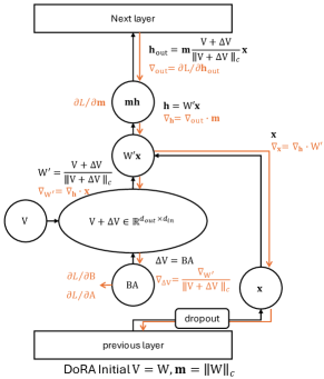
In Section 3, we explain that the memory usage of DoRA is significantly higher than that of LoRA due to its complex computation. We demonstrate the computation graph of DoRA here, as shown in Figure 3. DoRA decomposes into magnitude and direction and computes the final parameters matrix by . This complicated computation significantly increases memory usage because it requires caching a lot of intermediate values for computing gradients of , , and . As illustrated in Figure 3, each node passed by backpropagation stores some intermediate values for efficient gradient computing.
C.5 Cache Benefit
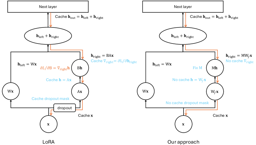
In the main context, we have already shown the memory cost of dropout layers in LoRA, in this section, we will discuss some other benefits of our approach. Figure 4 illustrates the computation and cache requirements in backpropagation (Rumelhart et al., 1986). For simplicity, we replace the notation with different . With the same number of trainable parameters, our approach eliminates the need to cache shown in the figure. While this benefit is negligible under lower rank settings () or when the number of fine-tuning layers is small, it becomes significant as the model size and rank settings increase. Although the caching requirement for can be addressed by recomputing during backpropagation, this would result in increased time complexity during training.
| Model, ft setting | mem | #param | ARC-c | ARC-e | BoolQ | HS | OBQA | PIQA | rte | SIQA | WG | Avg |
|---|---|---|---|---|---|---|---|---|---|---|---|---|
| Llama2(7B), LoRA, | 21.64GB | 40.0M(0.59%) | 44.71 | 76.89 | 77.49 | 57.94 | 32.2 | 78.73 | 60.65 | 47.59 | 68.75 | 60.55 |
| Llama2(7B), SPruFT, | 15.57GB | 36.4M(0.54%) | 43.34 | 77.43 | 77.80 | 57.06 | 32.2 | 78.02 | 63.18 | 46.52 | 69.14 | 60.52 |
| Llama2(7B), LoRA, | 22.21GB | 80.0M(1.19%) | 44.28 | 76.89 | 77.37 | 57.61 | 32.0 | 78.45 | 64.62 | 47.90 | 69.14 | 60.92 |
| Llama2(7B), SPruFT, | 16.20GB | 72.9M(1.08%) | 43.69 | 77.30 | 77.83 | 57.19 | 32.2 | 78.07 | 63.54 | 47.03 | 69.22 | 60.67 |
| Llama2(7B), LoRA, | 23.46GB | 159.9M(2.37%) | 44.97 | 77.02 | 77.43 | 57.75 | 32.0 | 78.45 | 62.09 | 47.75 | 68.75 | 60.69 |
| Llama2(7B), SPruFT, | 17.62GB | 145.8M(2.16%) | 43.60 | 77.26 | 77.77 | 57.47 | 32.6 | 78.07 | 64.98 | 46.67 | 69.30 | 60.86 |
| Llama2(7B), FA-LoRA, | 16.29GB | 23.2M(0.34%) | 44.54 | 77.36 | 77.83 | 57.39 | 30.8 | 77.69 | 67.15 | 47.08 | 68.82 | 60.96 |
| Llama2(7B), FA-SPruFT, | 14.16GB | 19.7M(0.29%) | 43.69 | 77.30 | 77.55 | 57.14 | 31.6 | 78.02 | 64.62 | 46.88 | 69.38 | 60.69 |
| Llama2(7B), FA-LoRA, | 16.56GB | 46.4M(0.69%) | 44.03 | 77.48 | 77.61 | 57.40 | 30.4 | 77.80 | 65.70 | 46.98 | 68.98 | 60.71 |
| Llama2(7B), FA-SPruFT, | 14.48GB | 39.3M(0.58%) | 43.77 | 77.26 | 77.65 | 57.17 | 31.8 | 78.07 | 65.70 | 46.78 | 69.22 | 60.82 |
| Llama2(7B), FA-LoRA, | 17.25GB | 92.8M(1.38%) | 43.77 | 77.57 | 77.74 | 57.45 | 31.0 | 77.86 | 66.06 | 47.13 | 69.06 | 60.85 |
| Llama2(7B), FA-SPruFT, | 15.21GB | 78.6M(1.17%) | 43.94 | 77.22 | 77.83 | 57.11 | 32.0 | 78.18 | 65.70 | 46.47 | 69.38 | 60.87 |
| Llama3(8B), LoRA, | 28.86GB | 41.9M(0.52%) | 53.50 | 81.44 | 82.35 | 60.61 | 34.2 | 79.87 | 69.31 | 48.00 | 73.56 | 64.76 |
| Llama3(8B), SPruFT, | 22.62GB | 39.8M(0.50%) | 51.19 | 80.81 | 81.10 | 60.21 | 34.4 | 79.60 | 70.40 | 47.19 | 73.01 | 64.21 |
| Llama3(8B), LoRA, | 29.37GB | 83.9M(1.04%) | 53.33 | 81.86 | 82.20 | 60.65 | 34.0 | 79.87 | 68.23 | 49.03 | 73.72 | 64.76 |
| Llama3(8B), SPruFT, | 23.23GB | 79.7M(0.99%) | 51.96 | 81.27 | 81.31 | 60.18 | 35.2 | 79.76 | 70.04 | 47.80 | 73.09 | 64.51 |
| Llama3(8B), LoRA, | 30.37GB | 167.8M(2.09%) | 53.07 | 81.40 | 82.32 | 60.67 | 34.2 | 79.98 | 69.68 | 48.52 | 73.56 | 64.82 |
| Llama3(8B), SPruFT, | 24.49GB | 159.4M(1.98%) | 52.47 | 81.10 | 81.28 | 60.29 | 34.6 | 79.76 | 70.04 | 47.75 | 73.24 | 64.50 |
| Llama3(8B), FA-LoRA, | 23.54GB | 28.3M(0.35%) | 51.45 | 81.48 | 82.17 | 60.17 | 34.4 | 79.60 | 68.95 | 47.75 | 73.48 | 64.38 |
| Llama3(8B), FA-SPruFT, | 21.24GB | 23.1M(0.29%) | 50.60 | 80.85 | 81.19 | 60.22 | 34.2 | 79.54 | 70.76 | 47.24 | 73.01 | 64.18 |
| Llama3(8B), FA-LoRA, | 23.89GB | 56.6M(0.71%) | 52.22 | 81.61 | 82.35 | 60.26 | 35.0 | 79.98 | 69.68 | 48.41 | 73.80 | 64.81 |
| Llama3(8B), FA-SPruFT, | 21.62GB | 46.1M(0.57%) | 51.79 | 81.06 | 81.22 | 60.20 | 35.2 | 79.65 | 71.48 | 47.24 | 73.16 | 64.56 |
| Llama3(8B), FA-LoRA, | 24.55GB | 113.2M(1.41%) | 52.47 | 81.36 | 82.23 | 60.17 | 35.0 | 79.76 | 70.04 | 48.31 | 73.56 | 64.77 |
| Llama3(8B), FA-SPruFT, | 22.41GB | 92.3M(1.15%) | 52.22 | 81.19 | 81.35 | 60.20 | 34.2 | 79.71 | 69.31 | 47.13 | 73.01 | 64.26 |
| Model, ft setting | ARC-c | ARC-e | BoolQ | HS | OBQA | PIQA | rte | SIQA | WG | Avg |
|---|---|---|---|---|---|---|---|---|---|---|
| Llama2(7B), SPruFT | ||||||||||
| , random | 43.34 | 76.43 | 77.83 | 57.18 | 31.4 | 78.13 | 62.45 | 45.80 | 69.30 | 60.21 |
| , | 43.34 | 77.43 | 77.80 | 57.06 | 32.2 | 78.02 | 63.18 | 46.52 | 69.14 | 60.52 |
| , ZOTaylor | 43.43 | 77.44 | 77.49 | 57.79 | 32.0 | 78.35 | 64.26 | 46.67 | 68.90 | 60.70 |
| , random | 43.17 | 76.39 | 77.86 | 57.20 | 31.2 | 78.07 | 62.45 | 45.91 | 69.06 | 60.15 |
| , | 43.69 | 77.30 | 77.83 | 57.19 | 32.2 | 78.07 | 63.54 | 47.03 | 69.22 | 60.67 |
| , ZOTaylor | 44.28 | 76.89 | 77.49 | 57.85 | 32.0 | 78.67 | 65.34 | 46.72 | 68.98 | 60.92 |
| , random | 43.34 | 76.30 | 77.80 | 57.22 | 31.2 | 78.07 | 63.18 | 45.96 | 69.22 | 60.25 |
| , | 43.60 | 77.26 | 77.77 | 57.47 | 32.6 | 78.07 | 64.98 | 46.67 | 69.30 | 60.86 |
| , ZOTaylor | 44.11 | 77.15 | 77.43 | 57.71 | 32.4 | 78.35 | 65.70 | 46.67 | 68.90 | 60.94 |
| , FA, random | 43.26 | 76.39 | 77.28 | 57.14 | 31.4 | 78.07 | 62.82 | 46.06 | 69.30 | 60.19 |
| , FA, | 43.69 | 77.30 | 77.55 | 57.14 | 31.6 | 78.02 | 64.62 | 46.88 | 69.38 | 60.69 |
| , FA, ZOTaylor | 44.20 | 77.61 | 77.22 | 57.41 | 31.8 | 78.07 | 65.70 | 46.72 | 68.90 | 60.85 |
| , FA, random | 43.34 | 76.30 | 77.52 | 57.18 | 31.4 | 78.07 | 62.82 | 46.01 | 69.14 | 60.20 |
| , FA, | 43.77 | 77.26 | 77.65 | 57.17 | 31.8 | 78.07 | 65.70 | 46.78 | 69.22 | 60.82 |
| , FA, ZOTaylor | 43.94 | 77.44 | 77.71 | 57.43 | 32.6 | 77.91 | 66.06 | 46.42 | 68.75 | 60.92 |
| , FA, random | 43.34 | 76.43 | 77.46 | 57.19 | 31.4 | 78.02 | 64.26 | 46.01 | 69.06 | 60.35 |
| , FA, | 43.94 | 77.22 | 77.83 | 57.11 | 32.0 | 78.18 | 65.70 | 46.47 | 69.38 | 60.87 |
| , FA, ZOTaylor | 44.45 | 77.82 | 77.74 | 57.41 | 31.4 | 77.80 | 66.06 | 46.57 | 68.59 | 60.87 |
| Llama3(8B), SPruFT | ||||||||||
| , random | 50.51 | 80.26 | 81.59 | 60.20 | 34.6 | 79.54 | 68.95 | 47.08 | 72.53 | 63.92 |
| , | 51.19 | 80.81 | 81.10 | 60.21 | 34.4 | 79.60 | 70.40 | 47.19 | 73.01 | 64.21 |
| , ZOTaylor | 50.94 | 81.61 | 82.42 | 60.17 | 35.6 | 79.60 | 70.40 | 47.19 | 73.40 | 64.59 |
| , random | 50.51 | 80.09 | 81.44 | 60.22 | 34.6 | 79.60 | 69.31 | 47.24 | 72.69 | 63.97 |
| , | 51.96 | 81.27 | 81.31 | 60.18 | 35.2 | 79.76 | 70.04 | 47.80 | 73.09 | 64.51 |
| , ZOTaylor | 52.13 | 81.14 | 82.32 | 60.19 | 35.6 | 79.82 | 70.04 | 47.03 | 73.01 | 64.59 |
| , random | 50.43 | 80.13 | 81.47 | 60.19 | 34.6 | 79.60 | 69.68 | 47.24 | 72.69 | 64.00 |
| , | 52.47 | 81.10 | 81.28 | 60.29 | 34.6 | 79.76 | 70.04 | 47.75 | 73.24 | 64.50 |
| , ZOTaylor | 52.22 | 81.99 | 82.54 | 60.13 | 34.6 | 79.76 | 70.04 | 47.59 | 73.16 | 64.67 |
| , FA, random | 50.43 | 80.05 | 81.47 | 60.19 | 34.6 | 79.65 | 69.68 | 47.03 | 72.85 | 63.99 |
| , FA, | 50.60 | 80.85 | 81.19 | 60.22 | 34.2 | 79.54 | 70.76 | 47.24 | 73.01 | 64.18 |
| , FA, ZOTaylor | 51.02 | 81.31 | 82.05 | 60.21 | 35.2 | 79.71 | 70.40 | 47.03 | 73.24 | 64.46 |
| , FA, random | 50.26 | 80.13 | 81.53 | 60.20 | 34.4 | 79.54 | 68.95 | 47.03 | 72.93 | 63.89 |
| , FA, | 51.79 | 81.06 | 81.22 | 60.20 | 35.2 | 79.65 | 71.48 | 47.24 | 73.16 | 64.56 |
| , FA, ZOTaylor | 51.71 | 81.31 | 82.05 | 60.22 | 34.8 | 79.65 | 69.68 | 47.29 | 72.77 | 64.39 |
| , FA, random | 50.26 | 80.09 | 81.47 | 60.22 | 34.6 | 79.71 | 69.31 | 47.08 | 72.85 | 63.95 |
| , FA, | 52.22 | 81.19 | 81.35 | 60.20 | 34.2 | 79.71 | 69.31 | 47.13 | 73.01 | 64.26 |
| , FA, ZOTaylor | 52.22 | 81.23 | 82.17 | 60.19 | 34.4 | 79.43 | 69.68 | 47.13 | 73.01 | 64.38 |
C.6 Rank Settings
We present an ablation study of rank settings here. Table 12 demonstrates that is sufficient for LoRA when fine-tuning Llama-2 and Llama-3. In contrast, increasing for our approach yields slight performance improvements. The most remarkable observation in Table 12 is the exceptional memory efficiency of our approach: even with , the memory usage of our method is significantly lower than that of LoRA with .
Table 13 is the full table of importance evaluation for Llama2 and Llama3.
C.7 Benefit of Freezing Attention Blocks
| Model, ft setting | mem | #param | ARC-c | ARC-e | BoolQ | HS | OBQA | PIQA | rte | SIQA | WG | Avg |
|---|---|---|---|---|---|---|---|---|---|---|---|---|
| Llama2(7B), LoRA, | 21.64GB | 40.0M(0.59%) | 44.71 | 76.89 | 77.49 | 57.94 | 32.2 | 78.73 | 60.65 | 47.59 | 68.75 | 60.55 |
| Llama2(7B), FA-LoRA, | 16.56GB | 46.4M(0.69%) | 44.03 | 77.48 | 77.61 | 57.40 | 30.4 | 77.80 | 65.70 | 46.98 | 68.98 | 60.71 |
| Llama2(7B), LoRA, | 22.21GB | 80.0M(1.19%) | 44.28 | 76.89 | 77.37 | 57.61 | 32.0 | 78.45 | 64.62 | 47.90 | 69.14 | 60.92 |
| Llama2(7B), FA-LoRA, | 17.25GB | 92.8M(1.38%) | 43.77 | 77.57 | 77.74 | 57.45 | 31.0 | 77.86 | 66.06 | 47.13 | 69.06 | 60.85 |
| Llama2(7B), SPruFT, | 15.57GB | 36.4M(0.54%) | 43.34 | 77.43 | 77.80 | 57.06 | 32.2 | 78.02 | 63.18 | 46.52 | 69.14 | 60.52 |
| Llama2(7B), FA-SPruFT, | 14.48GB | 39.3M(0.58%) | 43.77 | 77.26 | 77.65 | 57.17 | 31.8 | 78.07 | 65.70 | 46.78 | 69.22 | 60.82 |
| Llama2(7B), SPruFT, | 16.20GB | 72.9M(1.08%) | 43.69 | 77.30 | 77.83 | 57.19 | 32.2 | 78.07 | 63.54 | 47.03 | 69.22 | 60.67 |
| Llama2(7B), FA-SPruFT, | 15.21GB | 78.6M(1.17%) | 43.94 | 77.22 | 77.83 | 57.11 | 32.0 | 78.18 | 65.70 | 46.47 | 69.38 | 60.87 |
| Llama3(8B), LoRA, | 28.86GB | 41.9M(0.52%) | 53.50 | 81.44 | 82.35 | 60.61 | 34.2 | 79.87 | 69.31 | 48.00 | 73.56 | 64.76 |
| Llama3(8B), FA-LoRA, | 23.89GB | 56.6M(0.71%) | 52.22 | 81.61 | 82.35 | 60.26 | 35.0 | 79.98 | 69.68 | 48.41 | 73.80 | 64.81 |
| Llama3(8B), LoRA, | 29.37GB | 83.9M(1.04%) | 53.33 | 81.86 | 82.20 | 60.65 | 34.0 | 79.87 | 68.23 | 49.03 | 73.72 | 64.76 |
| Llama3(8B), FA-LoRA, | 24.55GB | 113.2M(1.41%) | 52.47 | 81.36 | 82.23 | 60.17 | 35.0 | 79.76 | 70.04 | 48.31 | 73.56 | 64.77 |
| Llama3(8B), SPruFT, | 22.62GB | 39.8M(0.50%) | 51.19 | 80.81 | 81.10 | 60.21 | 34.4 | 79.60 | 70.40 | 47.19 | 73.01 | 64.21 |
| Llama3(8B), FA-SPruFT, | 21.62GB | 46.1M(0.57%) | 51.79 | 81.06 | 81.22 | 60.20 | 35.2 | 79.65 | 71.48 | 47.24 | 73.16 | 64.56 |
| Llama3(8B), SPruFT, | 23.23GB | 79.7M(0.99%) | 51.96 | 81.27 | 81.31 | 60.18 | 35.2 | 79.76 | 70.04 | 47.80 | 73.09 | 64.51 |
| Llama3(8B), FA-SPruFT, | 22.41GB | 92.3M(1.15%) | 52.22 | 81.19 | 81.35 | 60.20 | 34.2 | 79.71 | 69.31 | 47.13 | 73.01 | 64.26 |
We now assess different fine-tuning strategies. Table 14 highlights the importance of selecting fine-tuning layers strategically to minimize redundant memory usage. Freezing the self-attention blocks achieves performance comparable to fine-tuning all layers while significantly reducing memory consumption during training. This efficiency stems from reducing the need to cache intermediate outputs for gradient computation. For example, as illustrated in Figure 4, using LoRA, must be cached to compute for the subsequent layer. Freezing the next layer eliminates this caching requirement, further optimizing memory usage.
Appendix D Details of Datasets
D.1 Vision Benchmarks
CIFAR100: CIFAR100 (Krizhevsky et al., 2009) has 100 classes with 600 images of size 32x32 per class, while the CIFAR10 has 10 classes with 6000 images per class. In this study, we use the CIFAR100 downloaded from huggingface (https://huggingface.co/datasets/uoft-cs/cifar100) with 500 training images and 100 validation images per class. In our experiments, we resize the images to 256x256, crop the center to 224x224, and normalize them using the CIFAR mean and standard deviation for the three channels.
Tiny-ImageNet: Tiny-ImageNet (Tavanaei, 2020) has 200 classes with images of size 64x64, while the full ImageNet-1k (Deng et al., 2009) has all 1000 classes where each image is the standard size 224x224. In this study, we use the Tiny-ImageNet downloaded from huggingface (https://huggingface.co/datasets/zh-plus/tiny-imagenet) with 500 training images and 50 validation images per class. In our experiments, we resize the images to 256x256, crop the center to 224x224, and normalize them using the mean and standard deviation for the three channels.
caltech101: Caltech101 (Li et al., 2022) consists of 101 classes, with images of varying sizes typically having edge lengths between 200 and 300 pixels. Each class contains approximately 40 to 800 images, resulting in a total of around 9,000 images. In this study, we use the Caltech101 dataset provided by PyTorch (https://pytorch.org/vision/main/generated/torchvision.datasets.Caltech101.html), allocating 75% of the images for training and the remaining 25% for validation. In our experiments, we preprocess the images by resizing them to 256×256, cropping the center to 224×224, and normalizing them using the mean and standard deviation for the three channels.
D.2 General Language Understanding Evaluation Benchmark (GLUE)
CoLA: The Corpus of Linguistic Acceptability (CoLA) is a dataset for assessing linguistic acceptability (Warstadt et al., 2018). This task is a binary classification for predicting whether a sentence is grammatically acceptable. The dataset is primarily from books and journal articles on linguistic theory.
MNLI: The Multi-Genre Natural Language Inference (MultiNLI) is a dataset designed to evaluate a model’s ability to perform natural language inference (NLI). The task is to predict whether the premise entails the hypothesis, contradicts the hypothesis, or neither. The data set contains 433k sentence pairs annotated with textual entailment information (Williams et al., 2018).
MRPC: The Microsoft Research Paraphrase Corpus (Dolan & Brockett, 2005) is a dataset designed for evaluating paraphrase detection systems. It consists of sentence pairs, with binary labels of whether the two sentences in the pair are equivalent. The data are automatically extracted from online news and labeled by humans.
QNLI: The Stanford Question Answering Dataset (SQuAD) is a dataset designed for machine comprehension of text (Rajpurkar et al., 2016). The dataset consists of question-paragraph pairs, where one of the sentences in the paragraph contains the answer to the corresponding question. The paragraphs are from Wikipedia and the questions are written by human annotators.
QQP: The Quora Question Pairs (QQP) dataset is a dataset of question pairs (https://data.quora.com/First-Quora-Dataset-Release-Question-Pairs). The task is to determine whether two questions are semantically equivalent.
RTE: The Recognizing Textual Entailment (RTE) datasets are a series of challenges that evaluate models’ ability to determine whether a premise can entail a given hypothesis (Dagan et al., 2006; Bar-Haim et al., 2006; Giampiccolo et al., 2007; Bentivogli et al., 2009). The data are constructed based on the texts from Wikipedia and news. The datasets have been used to evaluate the performance of both traditional language models and the state-of-the-art LLMs.
SST-2: The Stanford Sentiment Treebank is a dataset of sentences extracted from movie reviews (Socher et al., 2013). Each sentence is labeled as either positive or negative. The task is to predict whether the sentence is positive or negative.
STS-B: The Semantic Textual Similarity Benchmark (STSB) is a dataset with sentence pairs collected from news headlines, video and image captions, and natural language inference data (Cer et al., 2017). The task is to predict the semantic similarity between pairs of sentences. Each pair of sentences is annotated with a similarity score ranging from 0 to 5, where 0 indicates no semantic similarity and 5 indicates semantically equivalent.
D.3 Text-Generation Datasets
Stanford Alpaca: Alpaca is an instruction dataset designed for instruction training of pre-trained language models (Taori et al., 2023). It contains 52002 instruction-response pairs generated by OpenAI’s text-davinci-003 engine or written by humans. Note that there is only a training split in this dataset. Models fine-tuned on Alpaca are often evaluated by other tasks like “EleutherAI LM Harness”.
ARC: The AI2 Reasoning Challenge (ARC) dataset consists of grade-school level, multiple-choice science questions (Clark et al., 2018). ARC dataset includes a Challenge Set and an Easy Set. The easy set contains questions that can be answered with straightforward reasoning, while the challenge set requires deeper understanding and more reasoning skills. The ARC-Easy includes 2251 training samples, 570 validation samples, and 2376 test samples and the ARC-Challenge includes 1119 training samples, 299 validation samples, and 1172 test samples.
BoolQ: Boolean Questions (BoolQ) is a dataset of yes/no question answering (Clark et al., 2019) and includes 9427 training samples and 3270 validation samples. The dataset is designed to assess models’ comprehension and reasoning abilities. Each example contains question, passage, answer, and title.
HellaSwag: HellaSwag is a dataset designed to evaluate the models’ abilities in generating reasonable contexts (Zellers et al., 2019). It consists of prompts with a short context followed by multiple possible continuations. The goal is to find the correct or most plausible option. The training set, validation set, and test set have 39905 samples, 10042 samples, 10003 samples, respectively.
OpenBookQA: OpenBookQA is a question-answering dataset (Mihaylov et al., 2018) comprising 4957 training samples, 500 validation samples, and 500 test samples. It requires reasoning ability and a deeper understanding of common knowledge to answer questions. Each data contains a short passage with multiple possible answers. The dataset emphasizes the integration of world knowledge and reasoning skills, making it a challenging benchmark for natural language processing models. It tests models’ abilities to understand and apply factual information effectively to solve problems.
WinoGrande: WinoGrande is a dataset of 44k problems for choosing the right option for a given sentence (Sakaguchi et al., 2021). It includes 40938 samples in the training set, 1,267 in the validation set, and 1,267 in the test set. The dataset is designed to assess models’ commonsense reasoning abilities. The examples contain sentences with fill-in-blanks that require the model to select the most appropriate option to complete the sentence.
SocialIQA: The SocialIQA dataset is a benchmark designed to evaluate a model’s ability to reason about social interactions, including understanding social dynamics, intentions, and the effects of human actions (Sap et al., 2019). SocialIQA includes 33410 samples in the training set and 1954 in the validation set.
PIQA: The PIQA (Physical Interaction Question Answering) dataset is a benchmark designed to evaluate a model’s ability to understand and reason about everyday physical interactions and affordances (Bisk et al., 2020). Here are some key details about PIQA: (Sakaguchi et al., 2021). PIQA contains 16113 samples in the training set and 1838 in the validation set.