Training-Free Guidance Beyond Differentiability:
Scalable Path Steering with Tree Search in Diffusion and Flow Models

Abstract

Training-free guidance enables controlled generation in diffusion and flow models, but most existing methods assume differentiable objectives and rely on gradients. This work focuses on training-free guidance addressing challenges from non-differentiable objectives and discrete data distributions. We propose an algorithmic framework TreeG: Tree Search-Based Path Steering Guidance, applicable to both continuous and discrete settings in diffusion and flow models. TreeG offers a unified perspective on training-free guidance: proposing candidates for the next step, evaluating candidates, and selecting the best to move forward, enhanced by a tree search mechanism over active paths or parallelizing exploration. We comprehensively investigate the design space of TreeG over the candidate proposal module and the evaluation function, instantiating TreeG into three novel algorithms. Our experiments show that TreeG consistently outperforms the top guidance baselines in symbolic music generation, small molecule generation, and enhancer DNA design, all of which involve non-differentiable challenges. Additionally, we identify an inference-time scaling law showing TreeG’s scalability in inference-time computation.

1 Introduction

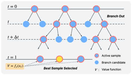
(a) Tree-Search Inference Process

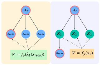
(b) Designs for BranchOut and Value Function $V$

Figure 1: Illustration of TreeG: (a) An active set of size $A$ is maintained, where each sample branches into $K$ candidates. At each step, the top $A$ candidates are selected, repeating until the final step where the best sample from the active set is chosen as the output. (b) Left: The current state-based (BranchOut, $V$) evaluates candidates via a lookahead estimate of the clean sample (Section 4.1). Right: The destination state-based design generates multiple predicted destination states and selects the optima (Section 4.2). The high-value destination state determines the next state. Gradient-based guidance can be applied to the current state-based branch-out module when a differentiable objective predictor is available (Section 4.3).

During the inference process of diffusion and flow models, guidance methods enable users to steer model generations toward desired objectives, achieving remarkable success across diverse domains such as vision (Dhariwal & Nichol, 2021; Ho & Salimans, 2022), audio (Kim et al., 2022), biology (Nisonoff et al., 2024; Zhang et al., 2024), and decision making (Ajay et al., 2022; Chi et al., 2023). In particular, training-free guidance offers high applicability by directly controlling the generation process with off-the-shelf objective functions without requiring additional training (Song et al., 2023; Zhao et al., 2024; Bansal et al., 2023; He et al., 2023). Most training-free guidance methods are gradient-based, as the gradient of the objective indicates a good direction for steering the inference (Ye et al., 2024; Guo et al., 2024), as a result, they rely on the assumptions that the objective function is differentiable.

However, recent advancements in generative models have broadened the playground of guided generation beyond differentiability: objectives of guidance have been enriched to include non-differentiable goals (Huang et al., 2024; Ajay et al., 2022); diffusion and flow models have demonstrated effectiveness in modeling discrete data (Austin et al., 2021; Vignac et al., 2022) for which objectives are inherently non-differentiable unless derived from differentiable features (Li et al., 2015; Yap, 2011). In those scenarios, those training-free guidance methods that are originally designed for differentiable objectives are limited by their assumptions. Yet, the design space beyond differentiability remains under-explored: only few methods exist (Lin et al., 2025; Huang et al., 2024), they are fundamentally different from each other and appear to be disconnected from the fundamental principles in previous guidance designs (Lin et al., 2025; Chung et al., 2022). Thus, it highlights the need of a unified perspective of and a comprehensive study on the design space of guidance beyond differentiability. To address this challenge, we propose an algorithmic framework TreeG: Tree Search-Based Path Steering Guidance, designed for both diffusion and flow models across continuous and discrete data spaces. TreeG consists of path steering guidance and a tree search mechanism.

Path steering guidance provides a unified perspective on training-free guidance beyond differentiability. Suppose

$$\bm{x}_{0},\cdots,\bm{x}_{t},\bm{x}_{t+\Delta t},\cdots,\bm{x}_{1}$$

denotes the inference process of a diffusion/flow model. While the gradient of the objective, when available, can offer a precise direction to steer inference at each step, an alternative is to discover a good inference path through a structured search process: proposing multiple $\bm{x}_{t+\Delta t}$’s as candidates for the next step (handled by a module BranchOut), evaluating them using some value function (denoted by $V$) that reflects the objective, and selecting the best candidate to move forward. The search procedure in TreeG is applicable beyond the differentiability assumption as it evaluates candidates with the zeroth-order information from the objective.

TreeG adopts a tree-search mechanism that enables search across multiple trajectories, further enhancing the performance of path steering guidance. An active set of size $A$ is maintained at each inference step, as shown in Figure 1(a). Each sample in the active set branches into multiple candidates next states, from which the top $A$ candidates—ranked by the value function $V$—are selected for the next step. This process iterates until the final step, where the best sample from the active set is chosen as the output. By scaling up the active set size $A$, TreeG can further improve objective function values as needed while adapting to the available computational budget.

The design space of TreeG is over the branching-out module and the value function, and TreeG is equipped with comprehensive design options. To ensure an effective search, two key considerations are efficient exploration and reliable evaluation. As illustrated in Figure 1(b), we propose two compatible pairs of $(\texttt{BranchOut},V)$, based on either the current state ($\bm{x}_{t}$), or the predicted destination state ($\hat{\bm{x}}_{1}$). The former uses the original diffusion model to generate multiple next states and employs a lookahead estimate of the clean sample for evaluation. The latter proposes multiple predicted destination states, which indicate the orientation of the next state, and selects the optimal using an off-the-shelf objective function. The next state is determined by the high-value destination state. In addition, TreeG introduces a novel gradient-based algorithm that enables the use of gradients to guide discrete flow models when a differentiable objective predictor is available.

(a) Symbolic Music Generation (Loss $\downarrow$)

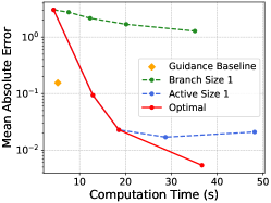
(b) Small Molecule Generation (MAE $\downarrow$)

(c) Enhancer DNA Design (Prob $\uparrow$)

Figure 2: TreeG outperforms the guidance baseline, with the optimization effect of the objective function following a scaling law with inference time. We compare TreeG with the strongest guidance baseline across tasks: Huang et al. (2024) for music generation and Nisonoff et al. (2024) for molecule and enhancer DNA tasks. Music generation involves a non-differentiable note density objective, while molecule and DNA tasks use discrete flow models. We evaluate TreeG with varying active set and branch-out sizes. “Optimal” refers to to the combination of active set and branch out sample sizes that achieves the best performance within the same inference time. The optimal line shows that TreeG outperforms the guidance baseline with a similar inference time.

The contributions of our paper are:

• We propose a novel framework TreeG of training-free guidance based on inference path search, applicable to both continuous and discrete, diffusion and flow models (Section 3). Our novel instantiated algorithms of TreeG (Section 4) tackle non-differentiability challenges from non-differentiable objectives or discrete-space models.

• We benchmark TreeG against existing guidance methods on three tasks: symbolic music generation (continuous diffusion with non-differentiable objectives), molecular design, and enhancer DNA design (both on discrete flow models). Path steering guidance, the special case of TreeG with the active set size 1, consistently outperforms the strongest guidance baseline (Figure 2 and Section 5.2). Our framework offers a suite of guidance options, with empirical results across three tasks suggesting that each task benefits the most from a guidance design that fits the nature of its objective and the underlying diffusion or flow model (Section 5.4).

• We discover an inference-time scaling law of TreeG, where performance gain of TreeG is observed as inference-time computation scales up with increasing active set and branch-out sizes (Figure 2 and Section 5.3).

2 Preliminaries

Notations.

Bold notation $\bm{x}$ denotes a high-dimensional vector, while $x$ represents a scalar. The superscript notation $x^{(d)}$ indicates the $d$-th dimension of the vector. In contrast, $x^{i}$ or $x^{i,j}$ denote independent samples with indices $i$ and $j$. $p_{t}$ is the density of intermediate distributions in training. For inference, $\mathcal{T}_{t}$ represents the sample distribution density or the rate matrix in the discrete case.

2.1 Diffusion and Flow Models.

Diffusion and flow models are trained by transforming the target data distribution into a prior noise distribution and learning to reverse the process. Let the data distribution be denoted as $p_{\text{data}}$, with $p_{1}=p_{\text{data}}$. During training, a sequence of intermediate distributions $p_{t}(t\in(0,1))$ is constructed to progressively transform the data distribution $p_{1}$ into a noise distribution $p_{0}$. Assume the total number of timesteps is $T$, resulting in a uniform interval $\Delta t=1/T$. The generation process begins with sampling $\bm{x}_{0}\sim p_{0}$. The model then iteratively generates $\bm{x}_{t}\sim p_{t}$ for timestep $t=i/T,$ where $i\in[T]$, ultimately producing $\bm{x}_{1}$ from the desired data distribution.

Diffusion and flow models are equivalent (Lipman et al., 2024; Domingo-Enrich et al., 2024). This paper focuses on the widely used continuous diffusion models and discrete flow models for continuous and discrete data, respectively, denoted as $u_{\theta}^{\textit{diff}}$ and $u_{\theta}^{\textit{flow}}$, abbreviated as $u_{\theta}$ when the context is clear. We collectively refer to the diffusion and flow models as the diffusion model. Below, we provide more detailed preliminaries on the two models.

Diffusion Models.

For diffusion models applied to continuous data, given a data sample $\bm{x}_{1}\sim p_{1}$, the noisy sample at timestep $t=i/T$ ($i\in[T]$) is constructed as $\bm{x}_{t}=\sqrt{\bar{\alpha}_{t}}\bm{x}_{1}+\sqrt{1-\bar{\alpha}_{t}}\epsilon$, where $\epsilon\sim\mathcal{N}\left(\bm{0},\bm{I}\right)$ and $\left\{\bar{\alpha}_{t}\right\}$ are pre-defined monotonically increasing parameters that control the noise level. The diffusion model $u_{\theta}^{\textit{diff}}:\mathcal{X}\times[0,1]\to\mathcal{X}$ parameterized by $\theta$, estimates the correspond clean state $\bm{x}_{1}$ of $\bm{x}_{t}$. The training objective is (Ho et al., 2020):

$$u_{\theta}^{\textit{diff}}=\mathop{\mathrm{argmin}}_{u_{\theta}}\mathbb{E}_{\bm{x}_{1}\sim p_{1},\epsilon}||u_{\theta}\left(\bm{x}_{t},t\right)-\bm{x}_{1}||^{2}=\mathbb{E}[\bm{x}_{1}\mid\bm{x}_{t}].$$ (1)

For sampling, we begin with $\bm{x}_{0}\sim\mathcal{N}\left(\bm{0},\bm{I}\right)$ and iteratively sample $\bm{x}_{t+\Delta t}\sim\mathcal{T}(\bm{x}_{t+\Delta t}\mid\bm{x}_{t})$. The sampling step proposed by DDPM (Ho et al., 2020) is:

$$\bm{x}_{t+\Delta t}=c_{t,1}\bm{x}_{t}+c_{t,2}u_{\theta}^{\textit{diff}}\left(\bm{x}_{t},t\right)+\sigma_{t}\epsilon,$$ (2)

where $\epsilon\sim\mathcal{N}\left(\bm{0},\bm{I}\right)$, $c_{t,1}=\frac{\sqrt{\alpha_{t}}(1-\bar{\alpha}_{t+\Delta t})}{1-\bar{\alpha}_{t}},c_{t,2}=\frac{\sqrt{\bar{\alpha}_{t+\Delta t}}(1-\alpha_{t})}{1-\bar{\alpha}_{t}}$ with $\alpha_{t}=\bar{\alpha}_{t}/\bar{\alpha}_{t+\Delta t}$ and $\sigma_{t}=\sqrt{1-\alpha_{t}}$.

Flow Models.

For flow models applied to discrete data, we follow the framework by Campbell et al. (2024). Suppose the discrete data space is $\mathcal{X}=[S]^{D}$, where $D$ is the dimension and $S$ is the number of states per dimension. An additional mask state $M$ is introduced as the noise prior distribution. Given a data sample $\bm{x}_{1}$, the intermediate distributions are constructed by $p_{t|1}(\bm{x}_{t}|\bm{x}_{1})=\Pi_{d=1}^{D}p_{t|1}(x_{t}|x_{1})$ with $p_{t|1}(x_{t}|x_{1})=t\delta\left\{x_{1},x_{t}\right\}+(1-t)\delta\left\{M,x_{t}\right\}$. The flow model $u_{\theta}^{\textit{flow}}$ estimates the true denoising distribution $p_{1|t}(\bm{x}_{1}|\bm{x}_{t})$. Specifically, it’s defined as $u_{\theta}^{\textit{flow}}=(u_{\theta}^{(1)},\ldots,u_{\theta}^{(D)})$, where each component $u_{\theta}^{(d)}(x_{1}|\cdot)$ is a function $\mathcal{X}\times[0,1]\to\Delta([S])$. Here, $\Delta([S])$ represents the probability distribution over the set $[S]$ The training objective is:

$$u_{\theta}^{\textit{flow}}=\mathop{\mathrm{argmin}}_{u_{\theta}}\mathbb{E}_{\bm{x}_{1}\sim p_{1},\bm{x}_{t}\sim p_{t|1}}\left[\log u_{\theta}^{(d)}(x_{1}^{(d)}|\bm{x}_{t})\right].$$ (3)

For generation, it requires the rate matrix:

$$R_{\theta,t}^{(d)}\left(\bm{x}_{t},j\right)=\mathbb{E}_{{x}_{1}^{(d)}\sim u_{\theta}^{(d)}\left({x}_{1}\mid\bm{x}_{t}\right)}\left[R_{t}\left(x_{t}^{(d)},j|x_{1}^{(d)}\right)\right],$$ (4)

where the pre-defined conditional rate matrix can be chosen as the popular: $R_{t}(x_{t},j|x_{1})=\frac{\delta\left\{j,x_{1}\right\}}{1-t}\left\{x_{t},M\right\}$. The generation process can be simulated via Euler steps (Sun et al., 2022):

$${x}_{t+\Delta t}^{(d)}\sim\text{Cat}\left(\delta\{{x}_{t}^{(d)},j\}+R_{\theta,t}^{(d)}\left(\bm{x}_{t},j\right)\Delta t\right),$$ (5)

where $\delta\left\{k,j\right\}$ is the Kronecker delta which is $1$ when $k=j$ and is otherwise $0$.

2.2 Training-free Guidance

The goal of training-free guidance is to enable conditional generation conditioned on some desired property. Suppose the property is evaluated by function $f$ and we consider both discrete and continuous $f$: $f(\bm{x})$ may represent discrete class label (e.g., $f$ is a classifier) or a real-valued output (e.g., $f$ a regression model or a zeroth-order oracle). Given a user-specified target $y$, the objective function $f_{y}$ quantifies how well the sample $\bm{x}$ aligns with $y$ by

• When $f(\bm{x})$ is an off-the-shelf classifier, the objective function is $f_{y}(\bm{x}):=\log f(y\mid\bm{x})$.

• When $f(\bm{x})$ is a regression model or a zeroth-order oracle, the objective function is $f_{y}(\bm{x}):=\log\exp^{-\frac{(y-f(\bm{x}))^{2}}{2\sigma^{2}}}=-\frac{(y-f(\bm{x}))^{2}}{2\sigma^{2}}$, assuming the true value of $\bm{x}$ is distributed as Gaussian centered at $f(\bm{x})$ with $\sigma$ being a fixed constant.

Based on the definition of $f_{y}$, a higher value indicates a more desirable sample. We refer to $f_{y}$ as an objective predictor when it is a differentiable neural network. We focus on training-free methods, which do not involve post-training $u_{\theta}$ or training a time-dependent classifier compatible with the diffusion noise scheduling.

2.3 Related Guidance Methods

We review the most related work to our paper here, please refer to Appendix A for other related works.

Nisonoff et al. (2024) and Lin et al. (2025) studies guidance for discrete flow models: the former follows classifier(-free) guidance method in Ho & Salimans (2022) and thus requires training time-dependent classifiers; the latter estimates the conditional rate by re-weighing the clean sample predictor $\bm{x}_{1}$ with their objective values in (4). (Huang et al., 2024) studies guiding continuous diffusion model with a non-differentiable objective and proposes a sampling approach, which is equivalent to our TreeG-SC algorithm with the active set size $A=1$. Though most guidance methods form a single inference path during generation, the idea of searching across multiple inference paths has also been touched upon by two concurrent works (Ma et al., 2025; Uehara et al., 2025). However, our TreeG provides the first systematical study of the design space of tree search, offering a novel methodology for both exploration and evaluation.

3 TreeG: Tree Search-Based Path Steering Guidance

While the gradient of the objective, when available, can offer a precise direction to steer inference (Guo et al., 2024), an alternative approach when the gradient in unavailable is to discover a good inference path through search: proposing multiple candidates for the next step, evaluating the candidates using some value function that reflects the objective, and selecting the best candidate to move forward. The search procedure is applicable beyond the differentiability assumption as it evaluates candidates with the zeroth-order information from the objective.

Based on this insight, we propose a framework that steers the inference path with search to achieve a targeted objective, by only leveraging the zeroth-order signals.

3.1 Algorithmic Framework

Let $\bm{x}_{0},\cdots,\bm{x}_{t},\bm{x}_{t+\Delta t},\cdots,\bm{x}_{1}$ denote the inference process transforming the pure noise state $\bm{x}_{0}$ to the clean sample state $\bm{x}_{1}$. In Alg. 1, at each step, path steering guidance uses the BranchOut module to propose $K$ candidate next states. The top candidates are then selected based on evaluations from the value function $V$ to proceed forward. The basic path steering guidance maintains a single path with one active sample at each step. However, the number of paths and active samples— the active set size $A$—can be scaled up for more efficient exploration through a tree-search mechanism.

1: Input: diffusion model $u_{\theta}$, branch out policy and value function $(\texttt{BranchOut},V)$, objective function $f_{y}$, active set size $A$, branch out sample size $K$.

2: Initialize: $t=0$, $\mathcal{A}=\left\{\bm{x}_{0}^{1},\ldots,\bm{x}_{0}^{A}\right\}$, $\bm{x}_{0}^{i}\sim p_{0}$.

3: while $t<1$ do

4:  Propose candidates for next step: For $\bm{x}_{t}^{i}\in\mathcal{A}$, $\bm{x}_{t+\Delta t}^{i,j}\sim\texttt{BranchOut}\left(\bm{x}_{t}^{i},u_{\theta}\right)$, $j\in[K]$.

5:  Selection: top $A$ candidates with respect to the value function $V\left(\bm{x}_{t+\Delta t}^{i,j},t,f_{y}\right)$, $i\in[A],j\in[K]$: $\bm{x}_{t+\Delta t}^{i_{1},j_{1}},\ldots,\bm{x}_{t+\Delta t}^{i_{A},j_{A}}$.

6:  Update the active set: $\mathcal{A}=\left\{\bm{x}_{t+\Delta t}^{i_{1},j_{1}},\ldots,\bm{x}_{t+\Delta t}^{i_{A},j_{A}}\right\}$

7:  $t\leftarrow t+\Delta t$.

8: end while

9: Output: $\bm{x}_{1}^{\ast}=\mathop{\mathrm{argmax}}_{\bm{x}_{1}\in\mathcal{A}}f_{y}\left(\bm{x}_{1}\right)$.

Algorithm 1 TreeG: Tree Search-Based Path Steering Guidance

In Alg. 1, the module BranchOut and the value function $V$ are two key components that require careful designs, for which we will present our novel designs in the next section. By specifying BranchOut and $V$, our framework gives rise to new algorithms demonstrating superior empirical performance to the existing baselines (Section 5). In addition, we will see that our framework unifies multiple existing training-free guidance methods (Section 4.4).

4 Design Space of TreeG

In this section, we will navigate through the design space of the TreeG algorithm, specifically the $(\texttt{BranchOut},V)$ pair. We propose two compatible $(\texttt{BranchOut},V)$ pairs, which operate by sampling and selecting either from the current state or the predicted destination state, respectively. We also propose a gradient-based discrete guidance method as a special case of TreeG.

4.1 Sample-then-Select on Current States

The idea for our first $(\texttt{BranchOut},V)$ pair is straightforward: sampling multiple realizations at the current state as candidates using the original generation process and selecting the one that leads to the most promising end state of the path. We define BranchOut for the current state as follows.

1: Input: $\bm{x}_{t}$, diffusion model $u_{\theta}$, time step $t$.

2: Sample the next state by the original generation process: $\bm{x}_{t+\Delta t}\sim$ (2) or (5).

3: Output: $\bm{x}_{t+\Delta t}$

Module 1 BranchOut-Current

To evaluate $\bm{x}_{t}$ (or $\bm{x}_{t+\Delta t}$), we propose using the value of $f_{y}$ at the end state if the generation process were to continue from this state. Specifically, for target $y$, we have

$$\log p_{t}(y\mid\bm{x}_{t}) =\log\mathbb{E}_{\bm{x}_{1}\sim p_{1|t}}[p(y\mid\bm{x}_{1})]$$ (6)

$$\simeq\mathbb{E}_{\bm{x}_{1}\sim p_{1|t}}[\log p(y\mid\bm{x}_{1})]$$

$$=\mathbb{E}_{\bm{x}_{1}\sim p_{1|t}}[f_{y}(\bm{x}_{1})],$$

where $f_{y}(\cdot)=\log p(y\mid\cdot)$ is the off-the-shelf objective operating in the clean space. Based on (6), we propose the value function for the current noisy states as follows.

1: Input: $\bm{x}_{t}$, diffusion model $u_{\theta}$, objective function $f_{y}$, time step $t$, (optional) Monte-Carlo sample size $N$.

2: Predict the clean sample: (continuous) $\hat{\bm{x}}_{1}=u_{\theta}(\bm{x}_{t},t)$. (discrete) $\hat{\bm{x}}_{1}^{i}\sim\text{Cat}\left(u_{\theta}(\bm{x}_{t},t)\right),i\in[N]$.

3: Evaluate: $V(\bm{x}_{t})=\frac{1}{N}\sum_{i=1}^{N}f_{y}({\hat{\bm{x}}_{1}^{i}})$.

4: Output: $V(\bm{x}_{t})$

Value Function 1 $V:$ Current State Evaluator

Note that we use the conditional expectation $u_{\theta}(\bm{x}_{t},t)=\mathbb{E}\left[\bm{x}_{1}\mid\bm{x}_{t}\right]$ as point estimation in Line 2 for the continuous case. Ye et al. (2024) observes that the point estimation yields a similar performance to the Monte Carlo estimation (Song et al., 2023) in continuous guidance. So for simplicity, we adopt the point estimation.

We refer to instantiating Algorithm 1 with Module 1 and value function 1 as TreeG-Sampling Current, abbreviated as TreeG-SC.

4.2 Sample-then-Select on Destination States

During inference, the transition probability in each step is determined by the current state and the end state of the path, which is estimated by the diffusion model, as stated in the following lemma (proof is in Appendix B).

Lemma 1.

In both continuous and discrete cases, the transition probability during inference at timestep $t$ satisfies:

$$\mathcal{T}(\bm{x}_{t+\Delta t}\mid\bm{x}_{t})=\mathbb{E}_{{\hat{\bm{x}}}_{1}}\left[\mathcal{T}^{\star}(\bm{x}_{t+\Delta t}\mid\bm{x}_{t},\hat{{\bm{x}}}_{1})\right],$$ (7)

where the expectation is taken over a distribution estimated by $u_{\theta}$, with $\mathcal{T}^{\star}$ being the true posterior distribution predetermined by the noise schedule.

In diffusion and flow models, $\mathcal{T}^{\star}$ is centered at a linear interpolation between its inputs: the current state $\bm{x}_{t}$, and the predicted destination state $\hat{{\bm{x}}}_{1}$, indicating that the orientation of the next state is partially determined by $\hat{\bm{x}}_{1}$, as it serves as one endpoint of the interpolation. If the $\hat{\bm{x}}_{t}$ has a high objective value, then its corresponding next state will be more oriented to a high objective. We define BranchOut for the destination state as follows.

1: Input: $\bm{x}_{t}$, diffusion model $u_{\theta}$, time step $t$, (optional) tuning parameter $\rho_{t}$.

2: Sample destination state candidates:  (continuous) $\hat{\bm{x}}_{1}\sim\mathcal{N}(u_{\theta}(\bm{x}_{t},t),\rho_{t}^{2}\bm{I})$. (discrete) $\hat{\bm{x}}_{1}\sim\text{Cat}\left(u_{\theta}(\bm{x}_{t},t)\right)$.

3: Compute the next state:  (continuous) $\bm{x}_{t+\Delta t}\sim\mathcal{N}\left(c_{t,1}\bm{x}_{t}+c_{t,2}\hat{\bm{x}}_{1},\sigma^{2}_{t}I\right)$. (discrete) ${x}_{t+\Delta t}^{(d)}\sim$ $\text{Cat}\left(\delta\{x_{t}^{(d)},j\}+R_{t}\left({x}_{t}^{(d)},j\mid\hat{x}_{1}^{(d)}\right)\Delta t\right)$.

4: Output: $(\bm{x}_{t+\Delta t},\bm{\hat{x}}_{1})$

Module 2 BranchOut-Destination

For the continuous diffusion model, the distribution to sample $\hat{\bm{x}}_{1}$ for is exploring around the point estimate $u_{\theta}(\bm{x}_{t},t)$, where $\rho_{t}$ is a tuning parameter. Implementation details for Algorithm 2 is in Section D.1. For $\bm{x}_{t+\Delta t}$ generated by BranchOut-Destination, we evaluate it by the objective value of its corresponding $\hat{\bm{x}}_{1}$.

1: Input: $(\bm{x}_{t+\Delta t},\bm{\hat{x}}_{1})$, objective function $f_{y}$.

2: Evaluate on the clean sample: $V\left((\bm{x}_{t+\Delta t},\bm{\hat{x}}_{1})\right)=f_{y}\left(\bm{\hat{x}}_{1}\right)$.

3: Output: $V\left((\bm{x}_{t+\Delta t},\bm{\hat{x}}_{1})\right)$

Value Function 2 $V:$ Destination State Evaluator

We name Algorithm 1 with Module 2 and Value Function 2 by TreeG-Sampling Destination (TreeG-SD).

4.3 Gradient-Based Guidance with Objective Predictor

Previously in this section, we derived two algorithms that do not rely on the gradient of objective. Though we do not assume the true objective is differentiable, when a differentiable objective predictor is available, leveraging its gradient as guidance is still a feasible option. Therefore, in what follows, we propose a novel gradient-based training-free guidance for discrete flow models, which also fits into the TreeG framework as a special case with $K=1$.

In a discrete flow model, sampling from the conditional distribution $p(\bm{x}\mid y)$ requires the conditional rate matrix $R_{t}(\bm{x}_{t},\cdot\mid y)$. (Nisonoff et al., 2024) derived the relation between the conditional and unconditional rate matrix:

$$R_{t}(\bm{x}_{t},j\mid y)=\frac{p_{t}(y\mid\bm{x}_{t}^{\backslash d}(j))}{p_{t}(y\mid\bm{x}_{t})}\cdot R_{t}(\bm{x}_{t},j),$$ (8)

where $\bm{x}_{t}^{\backslash d}$ matches $\bm{x}_{t}$ except at dimension $d$, and $\bm{x}_{t}^{\backslash d}(j)$ has its $d$-dimension set to $j$. $R_{t}(\bm{x}_{t},j)$ can be estimated by the rate matrix $R_{\theta,t}(\bm{x}_{t},j)$ computed from the flow model, so we only need to estimate the ratio $\frac{p_{t}(y\mid\bm{x}_{t}^{\backslash d}(j))}{p_{t}(y\mid\bm{x}_{t})}$, which further reduces to estimate $p_{t}(y\mid\bm{x})$ for any given $\bm{x}$. While Nisonoff et al. (2024) requires training a time-dependent predictor to estimate $p_{t}(y\mid\bm{x})$, we propose to estimate it using (6) in a training-free way. Here we restate:

$$\log p_{t}(y\mid\bm{x})\simeq\mathbb{E}_{\bm{x}_{1}\sim u_{\theta}}[f_{y}(\bm{x}_{1})]\simeq\frac{1}{N}\sum_{i=1}^{N}f_{y}({\hat{\bm{x}}_{1}^{i}}),$$ (9)

where $N$ is the Monte Carlo sample size and $\hat{\bm{x}}_{1}^{i}\sim\text{Cat}\left(u_{\theta}(\bm{x},t)\right),i\in[N]$. However, computing this estimation over all possible $\bm{x}_{t}^{\backslash d}$’s is computationally expensive. As suggested by Nisonoff et al. (2024); Vignac et al. (2022), we can approximate the ratio using Taylor expansion:

$$\log\frac{p_{t}(y\mid\bm{x}_{t}^{\backslash d})}{p_{t}(y\mid\bm{x}_{t})} ={\log p_{t}(y\mid\bm{x}_{t}^{\backslash d})}-{\log p_{t}(y\mid\bm{x}_{t})}$$ (10)

$$\simeq(\bm{x}_{t}^{\backslash d}-\bm{x}_{t})^{\top}\nabla_{\bm{x}_{t}}\log p_{t}(y\mid\bm{x}_{t}).$$

We apply the Straight-Through Gumbel-Softmax trick (Jang et al., 2016) to enable gradient backpropagation through the sampling process. Implementation details are provided in Section D.2, where we also verify this approximation has good accuracy compared to computing (9) for all $\bm{x}_{t}^{\backslash d}$’s, while enjoys higher efficiency. Combining the estimation from (9), we obtain our gradient-based training-free guidance for discrete flow and unify it into TreeG by defining the following BranchOut module, with its continuous counterpart:

1: Input: $\bm{x}_{t},t$, diffusion model $u_{\theta}$, differentiable predictor $f_{y}$, guidance strength $\gamma_{t}$, (optional) Monte-Carlo sample size $N$.

2: Compute the gradient guidance:  (continuous) $\bm{g}=\nabla_{\bm{x}_{t}}f_{y}(\hat{\bm{x}}_{1})$ with $\hat{\bm{x}}_{1}=u_{\theta}(\bm{x}_{t},t)$.  (discrete) $\bm{g}^{(d)}=(\bm{x}_{t}^{\backslash d}-\bm{x}_{t})^{\top}\nabla_{\bm{x}_{t}}\frac{1}{N}\sum_{i=1}^{N}f_{y}({\hat{\bm{x}}_{1}^{i}})$ with $\hat{\bm{x}}_{1}^{i}\sim\text{Cat}\left(u_{\theta}(\bm{x}_{t},t)\right),i\in[N]$.

3: Sample the next state:  (continuous) $\bm{x}_{t+\Delta t}=\gamma_{t}\bm{g}+c_{t,1}\bm{x}_{t}+c_{t,2}\hat{\bm{x}}_{1}+\sigma_{t}\epsilon$ with $\epsilon\sim\mathcal{N}\left(\bm{0},\bm{I}\right)$. (discrete) ${x}_{t+\Delta t}^{(d)}\sim$  $\text{Cat}\left(\delta\{x_{t}^{(d)},j\}+\exp(\gamma_{t}\bm{g}^{(d)})\odot R^{(d)}_{\theta,t}\left(\bm{x}_{t},j\right)\Delta t\right)$.

4: Output: $\bm{x}_{t+\Delta t}$

Module 3 BranchOut-Gradient

Algorithm 1 using BranchOut-Gradient with $K=1$ reduces to gradient-based guidance methods. When $K>1$, it is compatible with Value Function 1. We refer to this algorithm as TreeG Gradient (TreeG-G).

4.4 Analysis of TreeG

Generalizability of TreeG.

When the branch out size $K=1$ meaning there is no branching and all paths remain independent, TreeG-SC reduces to Best-of-N (Stiennon et al., 2020; Nakano et al., 2021). When the size of the active set $A=1$, TreeG-SC recovers the rule-based guidance in Huang et al. (2024) for continuous diffusion models. When $A=1,K=1$ with BranchOut-Gradient, it reduces to gradient-based guidance in continuous diffusion (Chung et al., 2022; Song et al., 2023).

Computational Complexity of TreeG.

To analyze the computational complexity of proposed algorithms, we define the following units of computation:

• $C_{\text{model}}$: the computational cost of passing through the diffusion or flow model.

• $C_{\text{pred}}$: the cost of calling the predictor.

• $C_{\text{backprop}}$: backpropagation through the diffusion model and predictor.

Let $N$ denote the Monte Carlo sample size used in Value Function 1. Recall $A$ is the active size and $K$ is the branch-out size. The computation complexity of TreeG is summarized in Table 1.

Methods	Computation
TreeG-SC	$AC_{\text{model}}+AK(C_{\text{model}}+NC_{\text{pred}})$
TreeG-SD	$AC_{\text{model}}+AKC_{\text{pred}}$
TreeG-G	$AK\left(C_{\text{model}}+NC_{\text{pred}}\right)+AC_{\text{backprop}}$

Table 1: Computation complexity of TreeG

Notice that the forward pass cost for the diffusion model in TreeG-SD is only $A$, compared to $AK$ for the other two methods. This is because it branches out at $\hat{\bm{x}}_{1}$ and directly evaluates $\hat{\bm{x}}_{1}$, eliminating the need to pass through the diffusion model. Thus, for the same $A,K$, TreeG-SD is more efficient.

5 Experiments

Base catogory	Method	Pitch histogram		Note density		Chord progression
		Loss $\downarrow$	OA $\uparrow$	Loss $\downarrow$	OA $\uparrow$	Loss $\downarrow$	OA $\uparrow$
Reference	No Guidance	$0.0180\pm 0.0100$	$0.842\pm 0.012$	$2.486\pm 3.530$	$0.830\pm 0.016$	$0.831\pm 0.142$	$0.854\pm 0.026$
Training-based	Classifier	$0.0050\pm 0.0040$	$0.855\pm 0.020$	$0.698\pm 0.587$	$\mathbf{0.861\pm 0.025}$	$0.723\pm 0.200$	$0.850\pm 0.033$
Training-free	DPS	$0.0010\pm 0.0020$	$0.849\pm 0.018$	$1.261\pm 2.340$	$0.667\pm 0.113$	$0.414\pm 0.256$	$0.839\pm 0.039$
	SCG	$0.0036\pm 0.0057$	$\mathbf{0.862\pm 0.008}$	$\mathbf{0.134\pm 0.533}$	$0.842\pm 0.022$	$0.347\pm 0.212$	$0.850\pm 0.046$
	TreeG-SD	$\mathbf{0.0002\pm 0.0003}$	$0.860\pm 0.016$	$0.142\pm 0.423$	$0.832\pm 0.023$	$\mathbf{0.301\pm 0.191}$	$\mathbf{0.856\pm 0.032}$

Table 2: Evaluation of guidance methods for music generation. TreeG-SD reduces loss by average $29.01\%$. Results for no guidance, Classifier, and DPS are copied from Huang et al. (2024). Due to computational limits, chord progression uses fewer inference steps with guidance (see Section E.1). The best results are bold, second best are underlined.

Base category	Method			$N_{r}^{*}=1$		$N_{r}^{*}=5$		$\mathrm{LogP}^{*}=-2$		$\mathrm{LogP}^{*}=10$
				MAE $\downarrow$	Validity $\uparrow$	MAE $\downarrow$	Validity $\uparrow$	MAE $\downarrow$	Validity $\uparrow$	MAE $\downarrow$	Validity $\uparrow$
Reference	No Guidance			$2.09\pm 1.16$		$2.03\pm 1.16$		$5.28\pm 1.59$		$6.72\pm 1.60$
Training-based	DG			$0.13\pm 0.35$	$9.73\%$	$0.20\pm 0.41$	$5.06\%$	$0.86\pm 0.65$	$9.29\%$	$1.66\pm 1.12$	$5.27\%$
Training-free	TFG-Flow			$0.28\pm 0.65$	$\textbf{13.61}\%$	$0.50\pm 0.64$	$5.70\%$	$1.86\pm 1.65$	$8.26\%$	$2.54\pm 1.92$	$\textbf{10.58}\%$
	TreeG-SC			$\textbf{0.03}\pm\textbf{0.26}$	$13.41\%$	$\textbf{0.12}\pm\textbf{0.53}$	$\textbf{6.83}\%$	$\textbf{0.68}\pm\textbf{0.60}$	$\textbf{10.27}\%$	$\textbf{1.65}\pm\textbf{1.83}$	$10.31\%$

Table 3: Evaluation on Small Molecule Generation (Targets: Number of Rings $N_{r}$ and Lipophilicity $\mathrm{LogP}$). The best is marked in bold. The validity of unguided generated sequences is $12.20\%$. The branch-out size for TreeG-SC is $K=2$.

Base category	Method (strength $\gamma$)		Class 1		Class 2		Class 3
			Prob $\uparrow$	FBD $\downarrow$	Prob $\uparrow$	FBD $\downarrow$	Prob $\uparrow$	FBD $\downarrow$
Reference	No Guidance		$0.007\pm 0.053$	$910$	$0.008\pm 0.052$	$602$	$0.021\pm 0.079$	$242$
Training-based	DG	$20$	$0.693\pm 0.264$	$\mathbf{102}$	$0.627\pm 0.340$	$\mathbf{120}$	$0.359\pm 0.188$	$\mathbf{109}$
		$100$	$0.173\pm 0.256$	$347$	$0.571\pm 0.356$	$212$	$0.372\pm 0.237$	$116$
		$200$	$0.064\pm 0.143$	$514$	$0.350\pm 0.351$	$294$	$0.251\pm 0.171$	$157$
Training-free	TFG-Flow	$200$	$0.004\pm 0.029$	$617$	$0.012\pm 0.076$	$352$	$0.054\pm 0.129$	$151$
	TreeG-G	$20$	$0.247\pm 0.280$	$314$	$0.313\pm 0.343$	$279$	$0.236\pm 0.178$	$111$
		$100$	$0.745\pm 0.217$	$125$	$0.915\pm 0.154$	$318$	$0.509\pm 0.242$	$189$
		$200$	$\mathbf{0.894\pm 0.136}$	$213$	$\mathbf{0.951\pm 0.110}$	$337$	$\mathbf{0.560\pm 0.258}$	$179$

Table 4: Evaluation of guidance methods for enhancer DNA design at varying guidance strength levels $\gamma_{t}=\gamma$ in Module Algorithm 3. The best is marked in bold, while the second best is underlined. The $x_{t}$ gradient method consistently achieves significantly higher target class probabilities, outperforming the training-free baseline method.

This section evaluates the performance of TreeG through experiments on one continuous and two discrete models across six tasks. It is structured as follows: Section 5.1 introduces the comparison methods; Section 5.2 details the tasks and results; Section 5.3 validates framework scalability and tree search effectiveness; and Section 5.4 discusses design choices for different scenarios.

5.1 Settings

Below are the methods we would like to compare:

For continuous models: DPS (Chung et al., 2022), a training-free classifier guidance method that relies on gradient computation and requires surrogate neural network predictors for non-differentiable objective functions; SCG (Huang et al., 2024), a gradient-free method and a special case of TreeG-SC with $A=1$; and TreeG-SD (Section 4.2).

For discrete models: DG (Nisonoff et al., 2024), a training-based classifier guidance requiring a predictor trained on noisy inputs, implemented with Taylor expansion and gradients; TFG-Flow (Lin et al., 2025), a training-free method estimating the conditional rate matrix; TreeG-G (Section 4.3), which trains a predictor on clean data for non-differentiable objectives; and TreeG-SC (Section 4.1) and TreeG-SD (Section 4.2).

For comparison with the above guidance methods in Section 5.2, the active size of TreeG is set to $A=1$. The results of scaling active set size $A$ and branch-out size $K$ are presented in Section 5.3.

5.2 Guided Generation

5.2.1 Symbolic music generation

We follow the setup of Huang et al. (2024), using a continuous diffusion model pre-trained on several piano midi datasets, detailed in Section E.1. The branch-out size for SCG and TreeG-SD is $K=16$.

Guidance Target.

Our study focuses on three types of targets: pitch histogram, note density, and chord progression. The objective function is $f_{y}(\cdot)=-\ell\left(y,\texttt{Rule}(\cdot)\right)$, where $\ell$ is the loss function. Notably, the rule function $\texttt{Rule}(\cdot)$ is non-differentiable for note density and chord progression.

Evaluation Metrics.

For each task, we evaluate performance on 200 targets as formulated by Huang et al. (2024). Two metrics are used: (1) Loss, which measures how well the generated samples adhere to the target rules. (2) Average Overlapping Area (OA), which assesses music quality by comparing the similarity between the distributions of the generated and ground-truth music, focusing on matching target attributes (Yang & Lerch, 2020).

Results.

As shown in Table 2, our proposed TreeG-SD method demonstrates superior performance while maintaining comparable sample quality. For differentiable rules (pitch histogram), TreeG-SD outperforms DPS, which SCG, another gradient-free approach, cannot achieve. For non-differentiable rules such as note density and chord progression, TreeG-SD matches or exceeds SCG and significantly outperforms DPS.

5.2.2 Small molecule generation

We validate our methods on the generation of small molecules with discrete flow models. Following Nisonoff et al. (2024), the small molecules are represented as simplified molecular-input line-entry system (SMILES) strings. These discrete sequences are padded to 100 tokens and there are 32 possible token types including one pad and one mask token $M$. We adopt the same unconditional flow model and Euler sampling curriculum as Nisonoff et al. (2024).

Guidance Target. Achieving expected chemical properties, i.e., number of rings $N_{r}$ or lipophilicity $\mathrm{LogP}$, is the goal of guided generation. These two properties of SMILES sequences could be evaluated through an open-source analysis tool RDKit (Landrum, 2013). We choose $N_{r}^{*}=[0,6]$ and $\mathrm{LogP}^{*}=[-2,0,2,4,6,8,10]$ as target values. The predictor used for guidance would be $f_{y}(\bm{x})=-\frac{(y-f(\bm{x}))^{2}}{2\sigma^{2}}$.

Evaluation Metrics. We evaluate the mean absolute error (MAE) between the target values and the properties of 1000 generated valid unique sequences, which are measured by RDKit. Besides, we take the validity of generated sequences, i.e., the ratio of valid unique sequences within all generated sequences, as a metric to compare different methods under the same target value.

Results. Compared with the training-based classifier guidance method DG, our sampling method TreeG-SC consistently achieves lower MAE and higher validity for both two properties as shown in Table 3. In addition, TreeG-SC outperforms TFG-Flow, which is also a training-free guidance method, by a large margin in terms of MAE, while maintaining comparable or better validity. On average, TreeG-SC achieves a relative performance improvement of $39.44\%$ on $N_{r}$ and $19.45\%$ on $\mathrm{LogP}$ compared to the best baseline DG. Please refer to Table 11 for details.

5.2.3 Enhancer DNA design

We follow the experimental setup of Stark et al. (2024), using a discrete flow model pre-trained on DNA sequences of length 500, each labeled with one of 81 cell types (Janssens et al., 2022; Taskiran et al., 2024). For inference, we apply 100 Euler sampling steps. The branch-out size for gradient guidance TreeG-G is $K=1$.

Guidance Target.

The goal is to generate enhancer DNA sequences that belong to a specific target cell type. The guidance target predictor is provided by an oracle classifier $f$ from Stark et al. (2024). The objective function of given cell class $y$ is $f_{y}(\cdot)=\log f(y\mid\cdot)$.

Evaluation Metrics.

We generate 1000 DNA sequences given the cell type. Performance is evaluated using two metrics. The first is Target Class Probability, provided by the oracle classifier, where higher probabilities indicate better guidance. The second metric, Frechet Biological Distance (FBD), measures the distributional similarity between the generated samples and the training data for a specific target class (i.e., class-conditioned FBD), with lower values indicating better alignment.

Results.

Table 4 shows class-conditioned enhancer DNA generation results. Our TreeG-G consistently achieves the highest target probabilities as $\gamma$ increases compared to the training-based baseline DG. The training-free baseline, TFG-Flow, shows almost no guidance effect with increased strength or Monte Carlo sampling. See Appendix F for details.

5.3 Scalability of TreeG

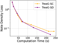
(a) Note Density (Music)

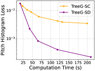
(b) Pitch Histogram (Music)

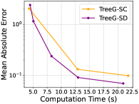
(c) Molecular Design ($N_{r}^{*}=5$)

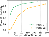
(d) Enhancer DNA (Class 4)

Figure 3: Inference Time Scaling Behavior: As the active set size and branch-out size increase, the optimization effect of the objective function scales with inference time. This trend is consistently observed across all algorithms and tasks. The inference time is measured with a batch size of 1 for music and 100 for molecule and DNA design. For DNA design, $\gamma=20$ for TreeG-G.

Our TreeG is scalable to the active size $A$ (i.e., the number of generation paths) and the branch-out size $K$. It is compatible with all guidance methods. This section demonstrates that increasing $A$ and $K$ consistently enhances the objective function’s value.

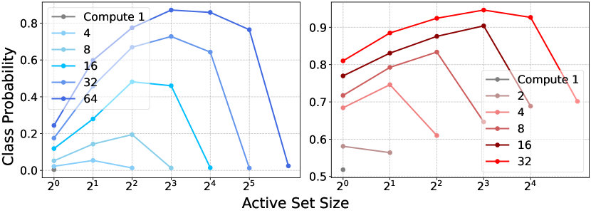
Figure 4: Trade-off between Active Set Size $A$ and Branch-out Size $K$ with Fixed Compute. TreeG-SC and TreeG-G vary $(A,K)$ with fixed total compute $A*K$ for enhancer DNA design. Performance peaks when $A$ and $K$ are in the moderate range. The results are for Class 4 and $\gamma=20$ for TreeG-G.

Scalability on Inference-time Computation.

When increasing the active set size and branch-out size, the computational cost of inference rises. We investigate the performance frontier to optimize the objective function concerning inference time. The results reveal an inference-time scaling law, as illustrated in Figure 3. Our findings indicate consistent scalability across all algorithms and tasks, with Figure 3 showcasing four examples. Additional results refer to Appendix F.

Trade-off between Active Set Size $A$ and Branch-out Size $K$.

Table 1 shows the computational complexity of algorithms using BranchOut-Current, specifically TreeG-SC and TreeG-G, is $O(AK)$. Given a fixed product $A*K$ (i.e., fixed inference computation, detailed timing in Section F.3.2), we explore the optimal balance between $A$ and $K$. Figure 4 demonstrates that performance is highest when $A$ and $K$ are within a moderate range. Notably, in the special case where $K=1$, there is no branch-out or selection operation during inference, making it equivalent to the Best-of-N approach, which typically results in suboptimal performance.

5.4 Discussion on Design Axes

Based on the experiment results with $A=1$, we can compare the designs within TreeG along two axes. Gradient-free vs gradient-based guidance: TreeG-G is only effective when an accurate objective predictor exists. If so, then the choice is influenced by the latency in forward pass of the predictor — faster predictors benefit TreeG-SC and TreeG-SD, while slower ones make TreeG-G more practical. TreeG-SC (current state) vs TreeG-SD (destination state): results show TreeG-SC performs better than TreeG-SD for discrete flow; and vice versa for continuous diffusion. Please refer to Appendix C for a more detailed discussion.

6 Conclusion

We proposed the framework TreeG based on inference path search, along with three novel instantiated algorithms: TreeG-SC, TreeG-SD, and TreeG-G, to address the non-differentiability challenge in training-free guidance. Experimental results demonstrated the improvements of TreeG against existing methods. Furthermore, we identified an inference-time scaling law that highlights TreeG’s scalability in inference-time computation.

Impact Statement

This paper aims to advance control techniques in generative AI and contribute to the broader field of Machine Learning. Our research carries significant societal implications, with the potential to shape the ethical, technical, and practical applications of AI in profound ways.

Appendix A Additional Related Work

We provide more related work in this section.

Discrete diffusion and flow model.

Austin et al. (2021) and Hoogeboom et al. (2021) pioneered diffusion in discrete spaces by introducing a corruption process for categorical data. Campbell et al. (2022) extended discrete diffusion models to continuous time, while Lou et al. (2024) proposed learning probability ratios. Discrete Flow Matching Campbell et al. (2024); Gat et al. (2024) further advances this field by developing a Flow Matching algorithm for time-continuous Markov processes on discrete state spaces, commonly known as Continuous-Time Markov Chains (CTMCs). Lipman et al. (2024) presents a unified perspective on flow and diffusion.

Diffusion model alignment.

To align a pre-trained diffusion toward user-interested properties, fine-tuning the model to optimize a downstream objective function (Black et al., 2023; Uehara et al., 2024; Prabhudesai et al., 2023) is a common training-based approach. In addition to guidance methods, an alternative training-free approach involves optimizing the initial value of the reverse process (Wallace et al., 2023; Ben-Hamu et al., 2024; Karunratanakul et al., 2024). These methods typically use an ODE solver to backpropagate the objective gradient directly to the initial latent state, making them a gradient-based version of the Best-of-N strategy.

Appendix B Proof of Lemma 1

Proof.

For continuous cases, in the forward process, $\bm{x}_{t}\sim\mathcal{N}(\bar{\alpha}_{t}\bm{x}_{1},(1-\bar{\alpha}_{t})\bm{I}),\bm{x}_{t+\Delta t}\sim\mathcal{N}(\bar{\alpha}_{t+\Delta t}\bm{x}_{1},(1-\bar{\alpha}_{t+\Delta t})\bm{I})$, the posterior distribution is:

$$p\left(\bm{x}_{t+\Delta t}\mid\bm{x}_{t},\bm{x}_{1}\right)=\mathcal{N}\left(c_{t,1}\bm{x}_{t}+c_{t,2}\bm{x}_{1},\beta_{t}\bm{I}\right),$$ (11)

where $\beta_{t}=\frac{1-\bar{\alpha}_{t+\Delta t}}{1-\bar{\alpha}_{t}}(1-\alpha_{t})$, and we recall $c_{t,1}=\frac{\sqrt{\alpha_{t}}(1-\bar{\alpha}_{t+\Delta t})}{1-\bar{\alpha}_{t}},c_{t,2}=\frac{\sqrt{\bar{\alpha}_{t+\Delta t}}(1-\alpha_{t})}{1-\bar{\alpha}_{t}}$.

We set $\mathcal{T^{\ast}}\left(\bm{x}_{t+\Delta t}\mid\bm{x}_{t},\bm{x}_{1}\right)=\mathcal{N}\left(c_{t,1}\bm{x}_{t}+c_{t,2}\bm{x}_{1},\beta_{t}\bm{I}\right)$ and the expectation $\hat{\bm{x}}$ taking over $q_{1}=N\left(u_{\theta}(\bm{x}_{t},t),(1-\alpha_{t})\bm{I}\right)$. It holds

$$\mathbb{E}_{{\hat{\bm{x}}}_{1}\sim q_{1}}\left[\mathcal{T}^{\ast}(\bm{x}_{t+\Delta t}\mid\bm{x}_{t},\hat{{\bm{x}}}_{1})\right]=\mathcal{N}\left(c_{t,1}\bm{x}_{t}+c_{t,2}\hat{\bm{x}}_{1},\sigma_{t}\bm{I}\right),$$ (12)

where we recall $\sigma_{t}=1-\alpha_{t}$. Therefore, (12) is exactly the distribution $\mathcal{T}(\bm{x}_{t+\Delta t}\mid\bm{x}_{t})$ for sampling during inference.

For discrete cases, $\mathcal{T}$ represents the rate matrix for inference sampling. We recall (4) the rate matrix for sampling during inference:

$$R_{\theta,t}^{(d)}\left(\bm{x}_{t},j\right)=\mathbb{E}_{{x}_{1}^{(d)}\sim u_{\theta}^{(d)}\left({x}_{1}\mid\bm{x}_{t}\right)}\left[R_{t}\left(x_{t}^{(d)},j|x_{1}^{(d)}\right)\right],$$

with the pre-defined conditional rate matrix $R_{t}(x_{t},j|x_{1})=\frac{\delta\left\{j,x_{1}\right\}}{1-t}\left\{x_{t},M\right\}$. Based on this, we have $\mathcal{T}^{\ast,(d)}(j\mid\bm{x}_{t})=R_{\theta,t}^{(d)}\left(\bm{x}_{t},j\right)$, and $\mathcal{T}^{(d)}(j\mid\bm{x}_{t},\bm{x}_{1})=R_{t}\left(x_{t}^{(d)},j|x_{1}^{(d)}\right)=\frac{\delta\left\{j,x_{1}\right\}}{1-t}\left\{x_{t},M\right\}$ is independent with the flow model $u_{\theta}$. Thus, they satisfy all requirements. We complete the proof.

∎

Appendix C Discussion on Design Axes

We compare the guidance designs: TreeG-SC, TreeG-SD and TreeG-G based on experimental results, to separate the effect of guidance design from the effect of tree search, we set $A=1$. A side-to-side comparison on the performance of the three methods are provided in Table 5.

Gradient-based v.s. Gradient-free: depends on the predictor

The choice between gradient-based and gradient-free methods largely depends on the characteristics of the predictor.

The first step is determining whether a reliable, differentiable predictor is available. If not, sampling methods should be chosen over gradient-based approaches. For example, in the chord progression task of music generation, the ground truth reward is obtained from a chord analysis tool in the music21 package (Cuthbert & Ariza, 2010), which is non-differentiable. Additionally, the surrogate neural network predictor achieves only $33\%$ accuracy (Huang et al., 2024). As shown in Table 2, in cases where no effective differentiable predictor exists, the performance of gradient-based methods (e.g., DPS) is significantly inferior to sampling-based methods (e.g., TreeG-SD and SCG).

If a good differentiable predictor is available, the choice depends on the predictor’s forward pass time. Our experimental tasks illustrate two typical cases: In molecule generation, where forward passes are fast as shown in Table 6, sampling approaches efficiently expand the candidate set and capture the reward signal, yielding strong results (Table 5). In contrast, for enhancer DNA design, where predictors have slow forward passes, increasing the sampling candidate set size to capture the reward signal becomes prohibitively time-consuming, making gradient-based method more effective (Table 5).

TreeG-SC v.s. TreeG-SD

Experiments on continuous data and discrete data give divergent results along this axis. In the continuous task of music generation (Table 2), TreeG-SD achieves equal or better performance than SCG (equivalent to TreeG-SC) with the same candidate size $K=16$ and similar time cost (details in Section F.1). Thus, TreeG-SD is preferable in this continuous setting. Conversely, for discrete tasks, TreeG-SD requires significantly more samples, while TreeG-SC outperforms it, as shown in Table 5.

		TreeG-G	TreeG-SC	TreeG-SD
Molecule	MAE $\downarrow$	$0.09\pm 0.54$	$0.02\pm 0.14$	$0.10\pm 0.33$
	Validity $\uparrow$	$13.10\%$	$14.03\%$	$2.60\%$
	Time $\downarrow$	13.5s	12.9s	11.2s
	$N$	30	30
	$K$		2	200
Enhancer	Prob $\uparrow$	$0.89\pm 0.14$	$0.13\pm 0.39$	$0.002\pm 0.000$
	FBD $\downarrow$	$213$	$384$	$665$
	Time $\downarrow$	10.3s	285.1s	189.7s
	$N$	20	20
	$K$		64	1024

Table 5: Comparison of results across TreeG-G, TreeG-SC and TreeG-SD. For molecule generation, the target is specified as the number of rings $N_{r}=2$. For enhancer DNA design, the results correspond to Class 1.

	$C_{\text{model}}$	$C_{\text{pred}}$	$C_{\text{backprop}}$
Molecule	0.038	2.2e-4	0.036
Enhancer	0.087	0.021	0.11

Table 6: Computation time per basic unit (ms)

Appendix D Implementation Details

D.1 Continuous Models

For TreeG-SD on the continuous case, we have two additional designs: the first one is exploring multiple steps when branching out a destination state; the second one is plugin Spherical Gaussian constraint(DSG) from (Yang et al., 2024). We present the case $A=1$ for TreeG-SD on the continuous case as follows while $A>1$ is similar.

1: Input: diffusion model $u_{\theta}$, objective function $f_{y}$, branch out sample size $K$, stepsize scale $\rho_{t}$, number of iteration $N_{\text{iter}}$

2: $t=0$, $\bm{x}_{0}\sim p_{0}$

3: while $t<1$ do

4:  Compute the predicted clean sample $\hat{\bm{x}}_{1}=u_{\theta}(\bm{x}_{t},t)$

5:  Set the branch out state $\bm{x}\leftarrow\hat{\bm{x}}_{1}$

6:  for $n=1,\dots,N_{\text{iter}}$ do

7:   Sample $\bm{x}^{i}=\bm{x}+\rho_{t}\bm{\xi}^{i}$, with $\bm{\xi}^{i}\sim\mathcal{N}\left(\bm{0},\bm{I}\right)$.

8:   Evaluate and select that maximizes the objective: $k=\mathop{\mathrm{argmax}}_{i}f_{y}\left(\bm{x}^{i}\right)$.

9:   Update $\bm{x}\leftarrow\bm{x}^{k}$.

10:  end for

11:  if DSG (Yang et al., 2024) then

12:   Compute the selected direction: $\bm{\xi}^{\ast}=\bm{x}-\hat{\bm{x}}_{1}$

13:   Rescale the direction: $\bm{\xi}^{\ast}\leftarrow\sqrt{D}\cdot\frac{\bm{\xi}^{\ast}}{||\bm{\xi}^{\ast}||}$, with $D=\text{dim}(\bm{x}_{t})$.

14:   Compute the next state: $\bm{x}_{t+\Delta t}=c_{t,1}\bm{x}_{t}+c_{t,2}\hat{\bm{x}}_{1}+\sigma_{t}\bm{\xi}^{\ast}$

15:  else

16:   Get the selected destination state $\hat{\bm{x}}_{1}\leftarrow\bm{x}$

17:   Sample the next state: $\bm{x}_{t+\Delta t}=c_{t,1}\bm{x}_{t}+c_{t,2}\hat{\bm{x}}_{1}+\sigma_{t}\epsilon$ with $\epsilon\sim\mathcal{N}\left(\bm{0},\bm{I}\right)$

18:  end if

19:  $t\leftarrow t+\Delta t$

20: end while

Algorithm 2 TreeG-SD (Continuous, $A=1$)

Notice that the computation complexity for using $N_{\text{iter}}$ step to select is: $AC_{\text{model}}+AKN_{\text{iter}}C_{\text{pred}}$. The setting of $N_{\text{iter}}$ will be provided in Section E.1.

D.2 Discrete Models

Estimate $\nabla_{\bm{x}_{t}}\log p_{t}(y\mid\bm{x}_{t})$. Since the sampling process of discrete data is genuinely not differentiable, we adopt the Straight-through Gumbel Softmax trick to estimate gradient while combining Monte-Carlo Sampling as stated in Equation 9. The whole process is listed in Module 4.

1: Input: $\bm{x}_{t},t$, diffusion model $u_{\theta}$, differentiable predictor $f_{y}$, Monte-Carlo sample size $N$, number of possible states $S$, Gumbel-Softmax temperature $\tau$

2: Sample $\hat{\bm{x}}_{1}^{i}\sim\text{Cat}\left(u_{\theta}(\bm{x}_{t},t)\right),i\in[N]$ with Gumbel Max and represent $x_{1}$ as an one-hot vector:

$$\hat{\bm{x}}_{1}^{i}=\arg\max_{j}(\log u_{\theta}(\bm{x}_{t},t)+g^{i}),$$ (13)

$g^{i}$ is a $S$-dimension Gumbel noise where $g_{j}\sim{\displaystyle{\text{Gumbel}}(0,1)},j\in[S]$.

3: Since the argmax operation is not differentiable, get the approximation $\hat{\bm{x}}_{1}^{i*}$ with softmax:

$$\hat{\bm{x}}_{1j}^{i*}=\frac{\mathrm{exp}((\log u_{\theta}(\bm{x}_{t},t)+g^{i}_{j})/\tau)}{\sum_{k}\mathrm{exp}((\log u_{\theta}(\bm{x}_{t},t)+g^{i}_{k})/\tau)},$$ (14)

4: Feed $\hat{\bm{x}}_{1}^{i}$ into the $f_{y}$ and obtain the gradient through backpropagation: $\nabla_{\hat{\bm{x}}_{1}^{i}}\log f_{y}(\hat{\bm{x}}_{1}^{i})$.

5: Straight-through Estimator: directly copy the gradient $\nabla_{\hat{\bm{x}}_{1}^{i}}\log f_{y}(\hat{\bm{x}}_{1}^{i})$ to $\hat{\bm{x}}_{1j}^{i*}$, i.e., $\nabla_{\hat{\bm{x}}_{1}^{i*}}\log f_{y}(\hat{\bm{x}}_{1}^{i*})\simeq\nabla_{\hat{\bm{x}}_{1}^{i}}\log f_{y}(\hat{\bm{x}}_{1}^{i})$.

6: Since Equation 14 is differentiable with regard to $x_{t}$, get $\nabla_{\bm{x}_{t}}\log p_{t}(y\mid\bm{x}_{t})\simeq\nabla_{\bm{x}_{t}}\frac{1}{N}\sum_{i=1}^{N}f_{y}({\hat{\bm{x}}_{1}^{i*}})$.

7: Output: $\nabla_{\bm{x}_{t}}\log p_{t}(y\mid\bm{x}_{t})$

Module 4 Gradient Approximation with Straight-Through Gumbel Softmax.

Appendix E Experimental Details

All experiments are conducted on one NVIDIA 80G H100 GPU.

E.1 Additional Setup for Symbolic Music Generation

Models.

We utilize the diffusion model and Variational Autoencoder (VAE) from (Huang et al., 2024). These models were originally trained on MAESTRO (Hawthorne et al., 2018), Pop1k7 (Hsiao et al., 2021), Pop909 (Wang et al., 2020), and 14k midi files in the classical genre collected from MuseScore. The VAE encodes piano roll segments of dimensions $3\times 128\times 128$ into a latent space with dimensions $4\times 16\times 16$.

Objective functions.

For the tasks of interest—pitch histogram, note density, and chord progression—the objective function for a given target $\bm{y}$ is defined as: $f_{\bm{y}}(\bm{x})=-\ell\left(\bm{y},\texttt{Rule}(\bm{x})\right)$, where $\texttt{Rule}(\cdot)$ represents a rule function that extracts the corresponding feature from $\bm{x}$, and $\ell$ is the loss function. Below, we elaborate on the differentiability of these objective functions for each task:

For pitch histogram, the rule function $\texttt{Rule-PH}(\cdot)$ computes the pitch histogram, and the loss function $\ell$ is the L2 loss. Since $\texttt{Rule-PH}(\cdot)$ is differentiable, the resulting objective function $f_{\bm{y}}^{\text{PH}}$ is also differentiable.

For note density, the rule function for note density is defined as: $\texttt{Rule-ND}(\bm{x})=\sum_{i=1}^{n}\mathbf{1}(x_{i}>\epsilon)$ where $\epsilon$ is a small threshold value, and $\mathbf{1}(\cdot)$ is the indicator function which makes $\texttt{Rule-ND}(\cdot)$ non-differentiable. $\ell$ is L2 loss. $f_{\bm{y}}^{\text{ND}}$ is overall non-differentiable.

For chord progression, the rule function $\texttt{Rule-CP}(\cdot)$ utilizes a chord analysis tool from the music21 package (Cuthbert & Ariza, 2010). This tool operates as a black-box API, and the associated loss function $\ell$ is a 0-1 loss. Consequently, the objective function $f_{\bm{y}}^{\text{CP}}$ is highly non-differentiable.

Test targets.

Our workflow follows the methodology outlined by Huang et al. (2024). For each task, target rule labels are derived from 200 samples in the Muscore test dataset. A single sample is then generated for each target rule label, and the loss is calculated between the target label and the rule label of the generated sample. The mean and standard deviation of these losses across all 200 samples are reported in Table 2.

Inference setup.

We use a DDPM with 1000 inference steps. Guidance is applied only after step 250.

Chord progression setup.

Since the objective function running by music21 package (Cuthbert & Ariza, 2010) is very slow, we only conduct guidance during 400-800 inference step.

TreeG-SD setup.

As detailed in Algorithm 2, we use DSG (Yang et al., 2024), and set $N_{\text{iter}}=2$ for pitch histogram and note density, $N_{\text{iter}}=1$ for chord progression. The stepsize $\rho_{t}=s\cdot\sigma_{t}/\sqrt{1+\sigma_{t}^{2}}$ (Song et al., 2023; Ye et al., 2024), with $s=2$ for pitch histogram, $s=0.5$ for note density and $s=1$ for chord progression.

E.2 Additional Setup for Small Molecule Generation

Due to lack of a differentiable off-the-shelf predictor, we train a regression model $f(\bm{x})$ on clean $x_{1}$ following the same procedure described in Nisonoff et al. (2024). Monte Carlo sample size for estimating $p_{t}(y\mid\bm{x}_{t})$ in TreeG-G and TreeG-SC is $N=30$ (Equation 9), and $N=200$ for TFG-Flow.

E.3 Additional Setup for Enhancer DNA Design

We test on eight randomly selected classes with cell type indices 33, 2, 0, 4, 16, 5, 68, and 9. For simplicity, we refer to these as Class 1 through Class 8.

We set the Monte Carlo sample size of TreeG-G and TreeG-SC as $N=20$, and $N=200$ for TFG-Flow.

Appendix F Additional Experiment Results

F.1 Additional Experiment Results for Symbolic Music Generation

F.1.1 Additional Information for Table 2

For the results in Table 2, the table presents a comparative improvement over the best baseline.

Task	Best baseline	TreeG-SD	Loss reduction
PH	$0.0010\pm 0.0020$ (DPS)	$0.0002\pm 0.0003$	$80\%$
ND	$0.134\pm 0.533$ (SCG)	$0.142\pm 0.423$	$-5.97\%$
CP	$0.347\pm 0.212$ (SCG)	$0.301\pm 0.191$	$13.26\%$
Average			$29.01\%$

Table 7: Improvement of TreeG-SD in music generation.

Both SCG and our TreeG-SD are gradient-free, which directly evaluates on ground truth objective functions. We provide the inference time of one generation for results in Table 2:

Task	SCG	TreeG-SD (ours)
PH	194	203
ND	194	204
CP	7267	6660

Table 8: Time(s) for SCG and TreeG-SD corresponding to results in Table 2.

F.1.2 Scalability

We conduct experiments scaling $A*K$ for TreeG-SD and TreeG-SC, where $A*K$ takes values $(1,2,4,8,16)$ for all combinations of $A$ and $K$ as $2^{i}$. Numerical results are in Table 9. Figure 5 shows the trade-off between $A$ and $K$.

Methods	($A$, $K$)	Loss $\downarrow$ (PH)	OA $\uparrow$ (PH)	Loss $\downarrow$ (ND)	OA $\uparrow$ (ND)
TreeG-SC	$(1,2)$	$0.0089\pm 0.0077$	$0.849\pm 0.017$	$0.506\pm 0.701$	$0.821\pm 0.060$
	$(2,1)$	$0.0145\pm 0.0082$	$0.848\pm 0.010$	$1.465\pm 1.842$	$0.850\pm 0.049$
	$(1,4)$	$0.0061\pm 0.00661$	$0.872\pm 0.015$	$0.232\pm 0.397$	$0.836\pm 0.039$
	$(2,2)$	$0.0067\pm 0.0073$	$0.862\pm 0.011$	$0.237\pm 0.559$	$0.832\pm 0.037$
	$(4,1)$	$0.0107\pm 0.0059$	$0.869\pm 0.021$	$1.139\pm 2.271$	$0.884\pm 0.021$
	$(1,8)$	$0.0049\pm 0.0069$	$0.861\pm 0.020$	$0.187\pm 0.467$	$0.831\pm 0.040$
	$(2,4)$	$0.0043\pm 0.0075$	$0.877\pm 0.016$	$0.158\pm 0.421$	$0.856\pm 0.014$
	$(4,2)$	$0.0040\pm 0.0051$	$0.865\pm 0.017$	$0.168\pm 0.688$	$0.845\pm 0.020$
	$(8,1)$	$0.0078\pm 0.0046$	$0.879\pm 0.008$	$0.784\pm 1.108$	$0.873\pm 0.021$
	$(1,16)$	$0.0036\pm 0.0057$	$0.862\pm 0.008$	$0.134\pm 0.533$	$0.842\pm 0.022$
	$(2,8)$	$0.0035\pm 0.0090$	$0.853\pm 0.012$	$0.100\pm 0.395$	$0.843\pm 0.029$
	$(4,4)$	$0.0035\pm 0.0095$	$0.832\pm 0.039$	$0.072\pm 0.212$	$0.841\pm 0.028$
	$(8,2)$	$0.0040\pm 0.0115$	$0.842\pm 0.022$	$0.071\pm 0.242$	$0.836\pm 0.016$
	$(16,1)$	$0.0061\pm 0.0032$	$0.882\pm 0.005$	$0.696\pm 1.526$	$0.884\pm 0.015$
TreeG-SD	$(1,2)$	$0.0022\pm 0.0021$	$0.869\pm 0.009$	$0.629\pm 0.827$	$0.826\pm 0.060$
	$(2,1)$	$0.0145\pm 0.0082$	$0.848\pm 0.010$	$1.465\pm 1.842$	$0.850\pm 0.049$
	$(1,4)$	$0.0008\pm 0.0008$	$0.853\pm 0.013$	$0.319\pm 0.619$	$0.815\pm 0.059$
	$(2,2)$	$0.0009\pm 0.0010$	$0.845\pm 0.015$	$0.231\pm 0.472$	$0.823\pm 0.045$
	$(4,1)$	$0.0107\pm 0.0059$	$0.869\pm 0.021$	$1.139\pm 2.271$	$0.884\pm 0.021$
	$(1,8)$	$0.0005\pm 0.0008$	$0.834\pm 0.018$	$0.217\pm 0.450$	$0.819\pm 0.050$
	$(2,4)$	$0.0004\pm 0.0005$	$0.816\pm 0.012$	$0.159\pm 0.401$	$0.841\pm 0.031$
	$(4,2)$	$0.0005\pm 0.0006$	$0.815\pm 0.020$	$0.113\pm 0.317$	$0.834\pm.023$
	$(8,1)$	$0.0078\pm 0.0046$	$0.879\pm 0.008$	$0.784\pm 1.108$	$0.873\pm 0.021$
	$(1,16)$	$0.0002\pm 0.0003$	$0.860\pm 0.016$	$0.142\pm 0.423$	$0.832\pm 0.023$
	$(2,8)$	$0.0002\pm 0.0003$	$0.814\pm 0.021$	$0.082\pm 0.266$	$0.845\pm 0.025$
	$(4,4)$	$0.0002\pm 0.0003$	$0.818\pm 0.013$	$0.048\pm 0.198$	$0.843\pm 0.012$
	$(8,2)$	$0.0003\pm 0.0004$	$0.808\pm 0.019$	$0.057\pm 0.179$	$0.820\pm 0.002$
	$(16,1)$	$0.0061\pm 0.0032$	$0.882\pm 0.005$	$0.696\pm 1.526$	$0.884\pm 0.015$

Table 9: Results of scaling $A*K$ of music generation.

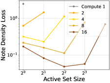
(a) TreeG-SD for ND

(b) TreeG-SD for PH

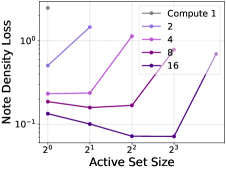
(c) TreeG-SC for ND

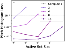
(d) TreeG-SC for PH

Figure 5: Trade-off between Active Set Size $A$ and Branch-out Size $K$ on Music Generation.

While $A*K$ represents the total computation to some extend, we know the different combination of $A$ and $K$ yields different costs even though $A*K$ is fixed, according to the computation complexity analysis Table 1. We provide true running time for one generation of the frontier of Figure 5 (a) and Figure 5 (b) at Table 10.

Note density		Pitch histogram
Time(s)	Loss	Time(s)	Loss
16.7	$2.486\pm 3.530$	16.7	$0.0180\pm 0.0100$
43.1	$0.629\pm 0.827$	42.2	$0.0022\pm 0.0021$
71.8	$0.231\pm 0.472$	65.3	$0.0008\pm 0.0008$
130.7	$0.113\pm 0.317$	118.6	$0.0004\pm 0.0005$
251.9	$0.057\pm 0.179$	209.6	$0.0002\pm 0.0003$

Table 10: Time and Loss of the optimal $(A,K)$ with fixed $A*K$ for TreeG-SD.

F.2 Additional Experiment Results for Small Molecule Generation

F.2.1 Additional Results for Table 3.

Method	$N_{r}$		$\mathrm{LogP}$
	MAE $\downarrow$	Validity $\uparrow$	MAE $\downarrow$	Validity $\uparrow$
DG	$-39.44\%$	$47.12\%$	$-19.45\%$	$11.53\%$
TFG-Flow	$-75.90\%$	$24.66\%$	$-44.76\%$	$1.38\%$

Table 11: Relative performance improvement of TreeG-SC compared to DG and TFG-Flow (average over different target values).

Base category	Method		$N_{r}^{*}=1$		$N_{r}^{*}=2$		$N_{r}^{*}=4$		$N_{r}^{*}=5$
			MAE $\downarrow$	Validity $\uparrow$	MAE $\downarrow$	Validity $\uparrow$	MAE $\downarrow$	Validity $\uparrow$	MAE $\downarrow$	Validity $\uparrow$
Reference	No Guidance		$2.09\pm 1.16$		$1.27\pm 1.02$		$1.27\pm 0.96$		$2.03\pm 1.16$
Training-based	DG		$0.13\pm 0.35$	$9.73\%$	$0.07\pm 0.27$	$10.77\%$	$0.08\pm 0.27$	$8.09\%$	$0.20\pm 0.41$	$5.06\%$
Training-free	TFG-Flow		$0.28\pm 0.65$	$13.61\%$	$0.20\pm 0.51$	$11.36\%$	$0.30\pm 0.53$	$8.15\%$	$0.50\pm 0.64$	$5.70\%$
	TreeG-G		$0.43\pm 1.18$	$\textbf{14.97}\%$	$0.09\pm 0.54$	$13.10\%$	$0.08\pm 0.46$	$10.82\%$	$0.25\pm 0.88$	$\textbf{7.60}\%$
	TreeG-SC		$\textbf{0.03}\pm\textbf{0.26}$	$13.41\%$	$\textbf{0.02}\pm\textbf{0.14}$	$\textbf{14.03}\%$	$\textbf{0.04}\pm\textbf{0.25}$	$\textbf{11.84}\%$	$\textbf{0.12}\pm\textbf{0.53}$	$6.83\%$
	TreeG-SD		$0.11\pm 0.38$	$2.91\%$	$0.10\pm 0.33$	$2.60\%$	$0.30\pm 0.58$	$1.31\%$	$0.67\pm 0.84$	$0.70\%$

Table 12: Small Molecule Generation (Target: Number of Rings $N_{r}$). Branch out sizes $K$ for TreeG-SC, TreeG-SD, and TreeG-G are $2,200$, and $1$ respectively while active set size $A$ is set as $1$ for all TreeG instantiations.

Base category	Method		$\mathrm{LogP}^{*}=-2$		$\mathrm{LogP}^{*}=0$		$\mathrm{LogP}^{*}=8$		$\mathrm{LogP}^{*}=10$
			MAE $\downarrow$	Validity $\uparrow$	MAE $\downarrow$	Validity $\uparrow$	MAE $\downarrow$	Validity $\uparrow$	MAE $\downarrow$	Validity $\uparrow$
Reference	No Guidance		$5.28\pm 1.59$		$3.32\pm 1.51$		$4.72\pm 1.60$		$6.72\pm 1.60$
Training-based	DG		$0.86\pm 0.65$	$9.29\%$	$0.65\pm 0.52$	$9.57\%$	$0.97\pm 0.76$	$10.42\%$	$1.66\pm 1.12$	$5.27\%$
Training-free	TFG-Flow		$1.86\pm 1.65$	$8.26\%$	$1.09\pm 1.03$	$8.77\%$	$1.53\pm 1.28$	$10.57\%$	$2.54\pm 1.92$	$10.58\%$
	TreeG-G		$1.37\pm 2.09$	$\textbf{13.13}\%$	$\textbf{0.55}\pm\textbf{0.45}$	$\textbf{13.51}\%$	$1.06\pm 1.78$	$\textbf{13.13}\%$	$5.05\pm 3.14$	$\textbf{11.24}\%$
	TreeG-SC		$\textbf{0.68}\pm\textbf{0.60}$	$10.27\%$	$0.58\pm 0.47$	$9.92\%$	$\textbf{0.70}\pm\textbf{0.91}$	$10.18\%$	$\textbf{1.65}\pm\textbf{1.83}$	$10.31\%$
	TreeG-SD		$1.73\pm 1.46$	$2.18\%$	$1.04\pm 0.94$	$2.07\%$	$1.37\pm 1.26$	$3.47\%$	$2.25\pm 1.89$	$4.11\%$

Table 13: Small Molecule Generation (Target: Lipophilicity $\mathrm{LogP}$). Branch out sizes $K$ for TreeG-SC, TreeG-SD, and TreeG-G are $2,200$, and $1$ respectively while active set size $A$ is set as $1$ for all TreeG instantiations.

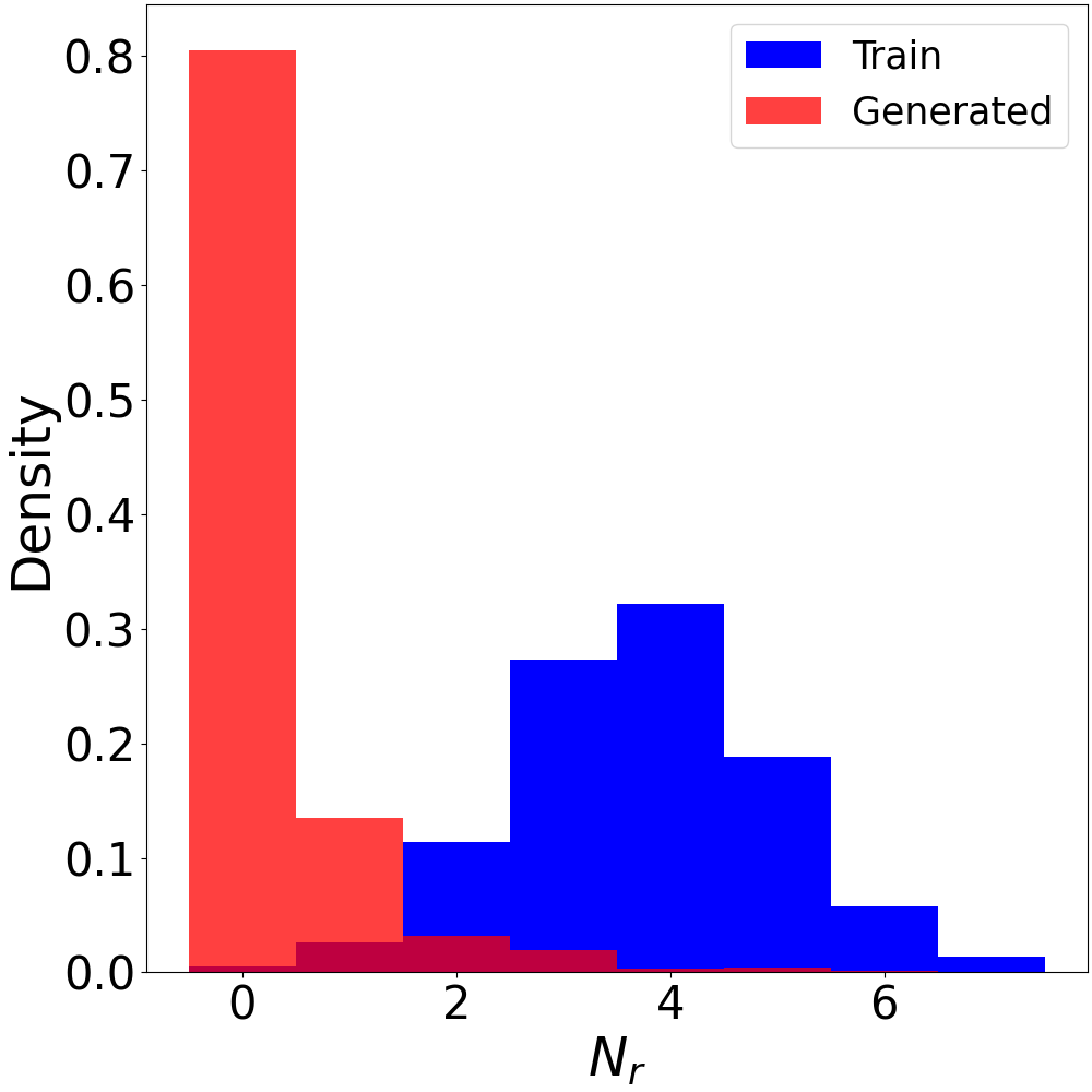
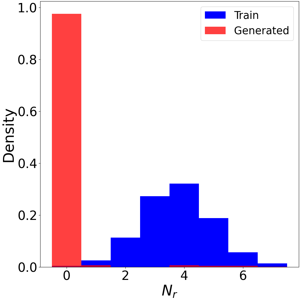
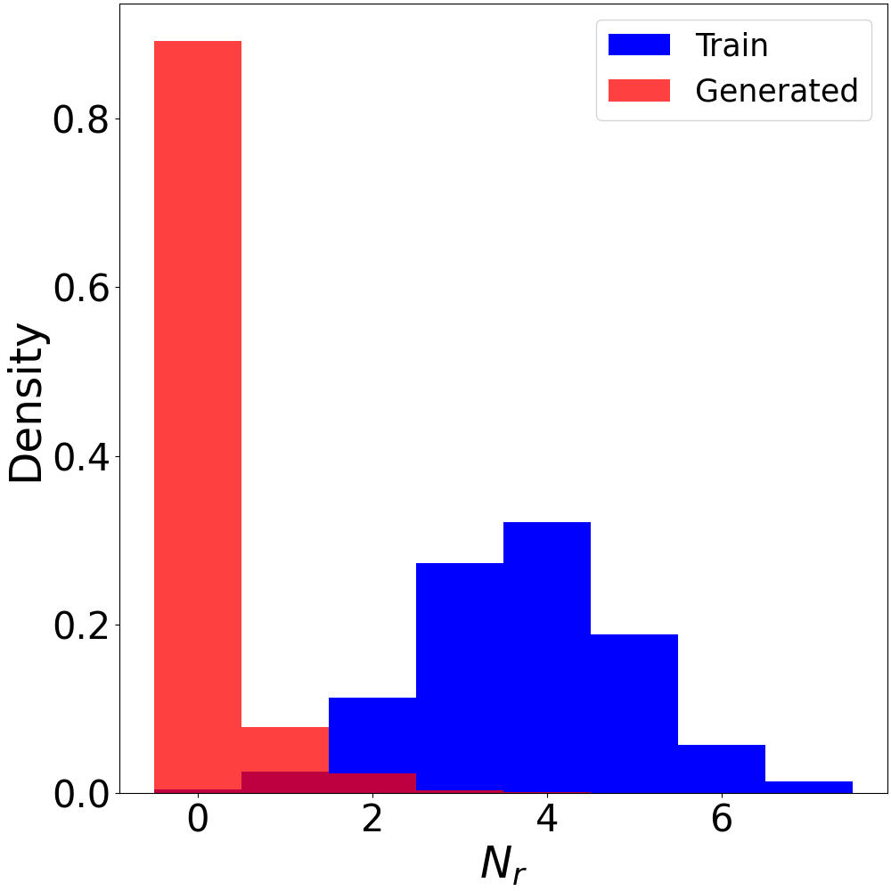
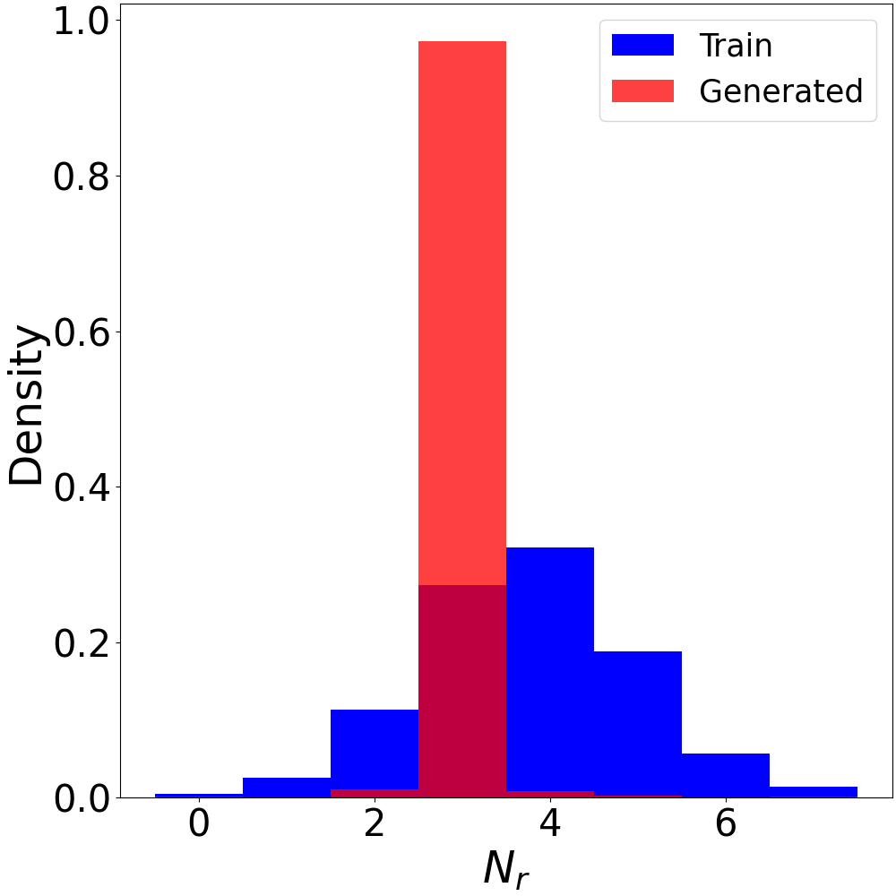
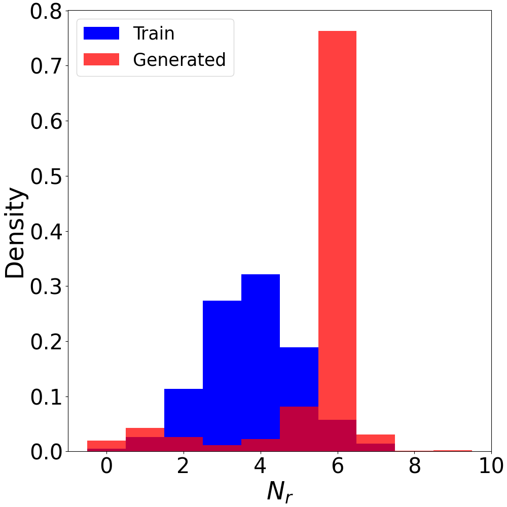
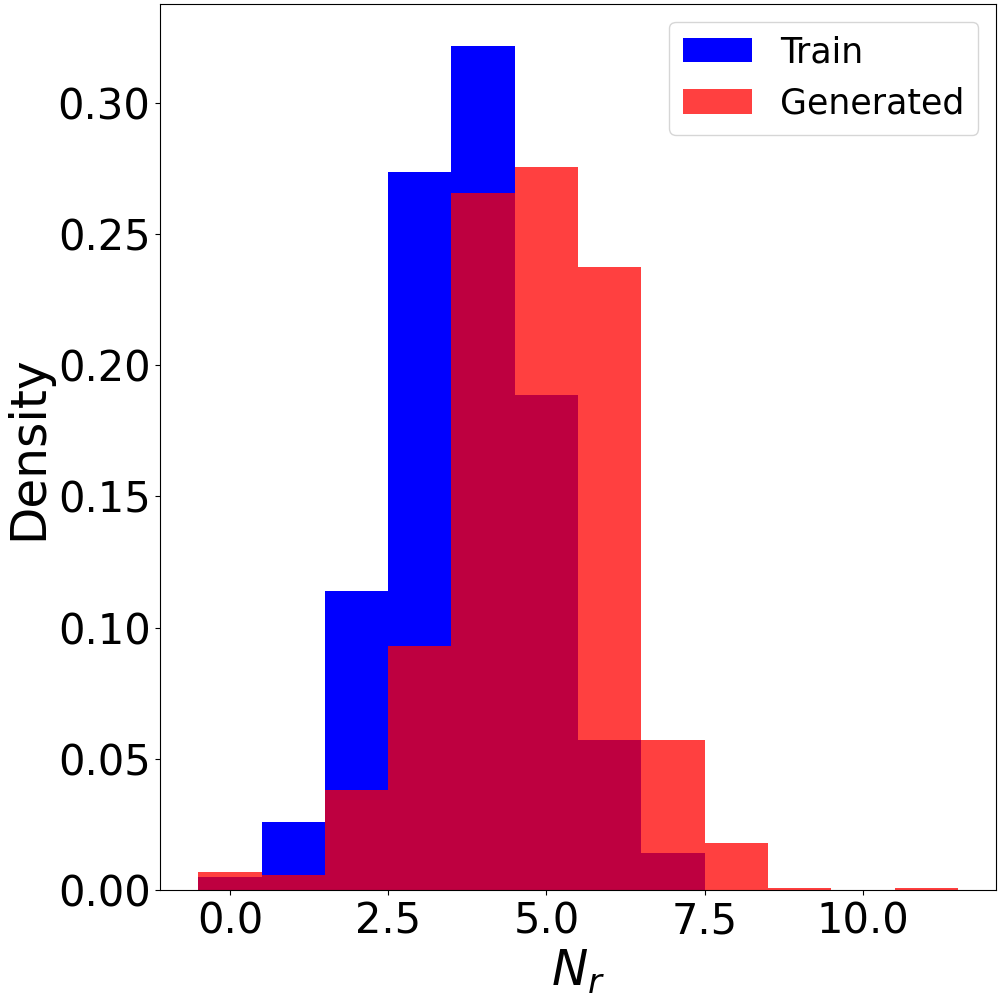
Figure 6: Distribution of $N_{r}$ in generated small molecules. The three rows correspond to different target values $N_{r}^{*}=0,3,6$. From left to right, each column represents different guidance methods (1) DG (2) TFG-Flow (3) TreeG-G (4) TreeG-SC (5) TreeG-SD. Blue blocks show the statistics of training dataset.

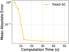
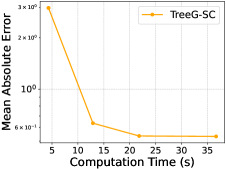
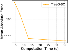
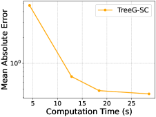
Figure 7: Small Molecule Generation: Scaling Law of TreeG-SC. From left to right, the targets are $N_{r}^{*}=3$, $N_{r}^{*}=6$, $\mathrm{LogP}^{*}=2$, $\mathrm{LogP}^{*}=8$.

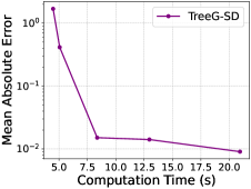
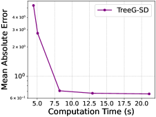
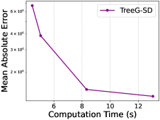
Figure 8: Small Molecule Generation: Scaling Law of TreeG-SD. From left to right, the targets are $N_{r}^{*}=1$, $N_{r}^{*}=5$, $\mathrm{LogP}^{*}=-2$, $\mathrm{LogP}^{*}=10$.

F.2.2 Scalability

We demonstrate the scaling laws for TreeG-SC and TreeG-SD in Figure 7 and Figure 8. Increasing computation time could boost guidance performance, i.e., lower mean absolute errors.

F.3 Additional Experiment Results for Enhancer DNA Design

F.3.1 Full Results of Table 4

Additional results of guidance methods for Class 4-8 are shown in Table 14. For both DG and our TreeG-G, we experiment with guidance values $\gamma\in[1,2,5,10,20,50,100,200]$ and compare the highest average conditional probability across the eight classes. On average, TreeG-G outperforms DG by $18.43\%$.

Method (strength $\gamma$)		Class 4		Class 5		Class 6		Class 7		Class 8
		Prob $\uparrow$	FBD $\downarrow$	Prob $\uparrow$	FBD $\downarrow$	Prob $\uparrow$	FBD $\downarrow$	Prob $\uparrow$	FBD	Prob $\uparrow$	FBD
No Guidance		$0.007\pm 0.059$	$446$	$0.035\pm 0.112$	$141$	$0.037\pm 0.115$	$179$	$0.010\pm 0.065$	$292$	$0.013\pm 0.073$	$478$
DG	$20$	$0.669\pm 0.377$	$57$	$0.665\pm 0.332$	$32$	$0.595\pm 0.334$	$26$	$0.693\pm 0.346$	$61$	$0.609\pm 0.350$	$95$
	$100$	$0.585\pm 0.380$	$132$	$0.466\pm 0.376$	$86$	$0.385\pm 0.334$	$84$	$0.475\pm 0.398$	$149$	$0.600\pm 0.342$	$326$
	$200$	$0.404\pm 0.384$	$140$	$0.199\pm 0.284$	$148$	$0.164\pm 0.235$	$132$	$0.208\pm 0.313$	$266$	$0.453\pm 0.370$	$362$
TFG-Flow	$200$	$0.015\pm 0.083$	$408$	$0.008\pm 0.048$	$267$	$0.033\pm 0.104$	$271$	$0.001\pm 0.015$	$371$	$0.006\pm 0.055$	$662$
TreeG-G	$20$	$0.518\pm 0.391$	$115$	$0.290\pm 0.306$	$61$	$0.250\pm 0.292$	$67$	$0.536\pm 0.335$	$137$	$0.159\pm 0.233$	$332$
	$100$	$0.845\pm 0.264$	$199$	$0.778\pm 0.279$	$123$	$0.843\pm 0.232$	$120$	$0.740\pm 0.365$	$161$	$0.413\pm 0.412$	$307$
	$200$	$0.826\pm 0.297$	$236$	$0.543\pm 0.426$	$104$	$0.364\pm 0.432$	$98$	$0.423\pm 0.457$	$177$	$0.073\pm 0.205$	$346$

Table 14: Additional results of the evaluation of guidance methods for enhancer DNA design.

F.3.2 Scalability

$A*K$ as a Computation Reference.

We use $A*K$ as the reference metric for inference time computation in TreeG-SC and TreeG-G, both employing BranchOut-Current. The corresponding inference times are shown in Figure 9, measured for a batch size of 100. Combinations of $(A,K)$ that yield the same $A*K$ value exhibit similar inference times. We exclude the case where $K=1$, as it does not require evaluation and selection, leading to a shorter inference time in practical implementation.

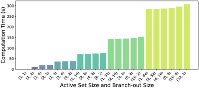
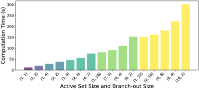
Figure 9: Inference Time for $(A,K)$ Combinations (Top: TreeG-SC; Bottom TreeG-G for DNA enhancer design). The $(A,K)$ combinations that yield the same $A*K$ value exhibit similar inference times. $K=1$ is excluded from this comparison since evaluation and selection are unnecessary in this case, leading to a shorter inference time in practical implementations.

We provide the scaling law of TreeG-G at different guidance strengths in Figure 10. The corresponding trade-off between $A$ and $K$ are shown in Figure 11. We also provide the scaling law and trade-off for TreeG-SC in Figure 12 and Figure 13, respectively.

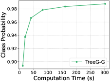
Figure 10: Enhancer DNA Design: Scaling Law of TreeG-G across Different Guidance Strengths: $\gamma=5,10,20,200$ from left to right (Class 1).

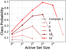
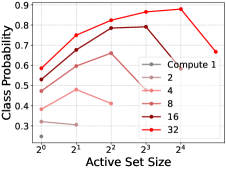
Figure 11: Enhancer DNA Design: Trade-off between $A$ and $K$ for TreeG-G. From left to right, guidance strengths are $\gamma=5,10,20,200$ (Class 1).

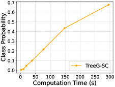
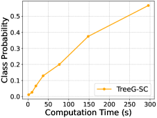
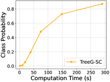
Figure 12: Enhancer DNA Design: Scaling Law of TreeG-SC, with Class 1 to 4 shown from left to right.

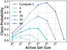
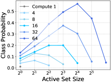
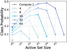
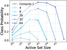
Figure 13: Enhancer DNA Design: Trade-off between $A$ and $K$ for TreeG-SC, with Class 1 to 4 shown from left to right.

Appendix G Ablation Studies

G.1 Symbolic Music Generation

For TreeG-SD, we ablation on $N_{\text{iter}}$ (detailed in Algorithm 2). As shown in Table 15, the loss decreases when $N_{\text{iter}}$ increases. However, increasing $N_{\text{iter}}$ also leads to higher computation costs. Here’s a trade-off between controllability and computation cost.

$N_{\text{iter}}$	Loss $\downarrow$ (PH)	OA $\uparrow$ (PH)	Loss $\downarrow$ (ND)	OA $\uparrow$ (ND)
1	$0.0031\pm 0.0037$	$0.733\pm 0.024$	$0.207\pm 0.418$	$0.810\pm 0.049$
2	$0.0005\pm 0.0008$	$0.833\pm 0.018$	$0.217\pm 0.450$	$0.819\pm 0.050$
4	$0.0005\pm 0.0006$	$0.786\pm 0.015$	$0.139\pm 0.319$	$0.830\pm 0.029$

Table 15: Ablation on $N_{\text{iter}}$ of TreeG-SD.

G.2 Discrete Models

Ablation on Taylor-expansion Approximation.

As shown in Table 16, using Taylor-expansion to approximate the ratio (Equation 10) achieve comparable model performance while dramatically improve the sampling efficiency compared to calculating the ratio by definition, i.e. TreeG-G-Exact.

Ablation on Monte Carlo Sample Size $N$.

As shown in Table 17, increasing the Monte Carlo sample size improves performance, but further increases in $N$ beyond a certain point do not lead to additional gains.

Method	$\mathrm{N_{r}}^{*}=1$			$\mathrm{N_{r}}^{*}=2$
	MAE $\downarrow$	Validity $\uparrow$	Time	MAE $\downarrow$	Validity $\uparrow$	Time
TreeG-G	$0.24\pm 0.76$	$19.23\%$	2.4min	$0.02\pm 0.14$	$13.51$	3.5min
TreeG-G-Exact	$0.00\pm 0.00$	$18.52\%$	356.9min	$0.02\pm 0.14$	$19.23\%$	345.2min

Table 16: Ablation on Taylor-expansion Approximation. The performances are evaluated on 50 generated samples.

$N$	$\mathrm{N_{r}}^{*}=2$		$\mathrm{N_{r}}^{*}=5$
	MAE $\downarrow$	Validity $\uparrow$	MAE $\downarrow$	Validity $\uparrow$
1	$0.47\pm 1.12$	$13.51\%$	$0.65\pm 1.37$	$8.83\%$
5	$0.30\pm 0.97$	$11.89\%$	$0.41\pm 1.14$	$7.61\%$
10	$0.17\pm 0.68$	$\textbf{14.20}\%$	$\textbf{0.20}\pm\textbf{0.76}$	$\textbf{8.87}\%$
20	$\textbf{0.09}\pm\textbf{0.46}$	$12.50\%$	$0.26\pm 0.91$	$7.81\%$
40	$0.10\pm 0.60$	$12.65\%$	$0.29\pm 1.01$	$8.58\%$

Table 17: Ablation on Monte Carlo Sample Size $N$. The performances are evaluated on 200 generated samples.

References

- Ajay et al. (2022) Ajay, A., Du, Y., Gupta, A., Tenenbaum, J., Jaakkola, T., and Agrawal, P. Is conditional generative modeling all you need for decision-making? arXiv preprint arXiv:2211.15657, 2022.
- Austin et al. (2021) Austin, J., Johnson, D. D., Ho, J., Tarlow, D., and Van Den Berg, R. Structured denoising diffusion models in discrete state-spaces. Advances in Neural Information Processing Systems, 34:17981–17993, 2021.
- Bansal et al. (2023) Bansal, A., Chu, H.-M., Schwarzschild, A., Sengupta, S., Goldblum, M., Geiping, J., and Goldstein, T. Universal guidance for diffusion models. In Proceedings of the IEEE/CVF Conference on Computer Vision and Pattern Recognition, pp. 843–852, 2023.
- Ben-Hamu et al. (2024) Ben-Hamu, H., Puny, O., Gat, I., Karrer, B., Singer, U., and Lipman, Y. D-flow: Differentiating through flows for controlled generation. arXiv preprint arXiv:2402.14017, 2024.
- Black et al. (2023) Black, K., Janner, M., Du, Y., Kostrikov, I., and Levine, S. Training diffusion models with reinforcement learning. arXiv preprint arXiv:2305.13301, 2023.
- Campbell et al. (2022) Campbell, A., Benton, J., De Bortoli, V., Rainforth, T., Deligiannidis, G., and Doucet, A. A continuous time framework for discrete denoising models. Advances in Neural Information Processing Systems, 35:28266–28279, 2022.
- Campbell et al. (2024) Campbell, A., Yim, J., Barzilay, R., Rainforth, T., and Jaakkola, T. Generative flows on discrete state-spaces: Enabling multimodal flows with applications to protein co-design. arXiv preprint arXiv:2402.04997, 2024.
- Chi et al. (2023) Chi, C., Xu, Z., Feng, S., Cousineau, E., Du, Y., Burchfiel, B., Tedrake, R., and Song, S. Diffusion policy: Visuomotor policy learning via action diffusion. The International Journal of Robotics Research, pp. 02783649241273668, 2023.
- Chung et al. (2022) Chung, H., Kim, J., Mccann, M. T., Klasky, M. L., and Ye, J. C. Diffusion posterior sampling for general noisy inverse problems. arXiv preprint arXiv:2209.14687, 2022.
- Cuthbert & Ariza (2010) Cuthbert, M. S. and Ariza, C. music21: A toolkit for computer-aided musicology and symbolic music data. In International Society for Music Information Retrieval, 2010.
- Dhariwal & Nichol (2021) Dhariwal, P. and Nichol, A. Diffusion models beat gans on image synthesis. Advances in neural information processing systems, 34:8780–8794, 2021.
- Domingo-Enrich et al. (2024) Domingo-Enrich, C., Drozdzal, M., Karrer, B., and Chen, R. T. Adjoint matching: Fine-tuning flow and diffusion generative models with memoryless stochastic optimal control. arXiv preprint arXiv:2409.08861, 2024.
- Gat et al. (2024) Gat, I., Remez, T., Shaul, N., Kreuk, F., Chen, R. T., Synnaeve, G., Adi, Y., and Lipman, Y. Discrete flow matching. arXiv preprint arXiv:2407.15595, 2024.
- Guo et al. (2024) Guo, Y., Yuan, H., Yang, Y., Chen, M., and Wang, M. Gradient guidance for diffusion models: An optimization perspective. arXiv preprint arXiv:2404.14743, 2024.
- Hawthorne et al. (2018) Hawthorne, C., Stasyuk, A., Roberts, A., Simon, I., Huang, C.-Z. A., Dieleman, S., Elsen, E., Engel, J., and Eck, D. Enabling factorized piano music modeling and generation with the maestro dataset. arXiv preprint arXiv:1810.12247, 2018.
- He et al. (2023) He, Y., Murata, N., Lai, C.-H., Takida, Y., Uesaka, T., Kim, D., Liao, W.-H., Mitsufuji, Y., Kolter, J. Z., Salakhutdinov, R., et al. Manifold preserving guided diffusion. arXiv preprint arXiv:2311.16424, 2023.
- Ho & Salimans (2022) Ho, J. and Salimans, T. Classifier-free diffusion guidance. arXiv preprint arXiv:2207.12598, 2022.
- Ho et al. (2020) Ho, J., Jain, A., and Abbeel, P. Denoising diffusion probabilistic models. Advances in neural information processing systems, 33:6840–6851, 2020.
- Hoogeboom et al. (2021) Hoogeboom, E., Nielsen, D., Jaini, P., Forré, P., and Welling, M. Argmax flows and multinomial diffusion: Learning categorical distributions. Advances in Neural Information Processing Systems, 34:12454–12465, 2021.
- Hsiao et al. (2021) Hsiao, W.-Y., Liu, J.-Y., Yeh, Y.-C., and Yang, Y.-H. Compound word transformer: Learning to compose full-song music over dynamic directed hypergraphs. In Proceedings of the AAAI Conference on Artificial Intelligence, volume 35, pp. 178–186, 2021.
- Huang et al. (2024) Huang, Y., Ghatare, A., Liu, Y., Hu, Z., Zhang, Q., Sastry, C. S., Gururani, S., Oore, S., and Yue, Y. Symbolic music generation with non-differentiable rule guided diffusion. arXiv preprint arXiv:2402.14285, 2024.
- Jang et al. (2016) Jang, E., Gu, S., and Poole, B. Categorical reparameterization with gumbel-softmax. arXiv preprint arXiv:1611.01144, 2016.
- Janssens et al. (2022) Janssens, J., Aibar, S., Taskiran, I. I., Ismail, J. N., Gomez, A. E., Aughey, G., Spanier, K. I., De Rop, F. V., Gonzalez-Blas, C. B., Dionne, M., et al. Decoding gene regulation in the fly brain. Nature, 601(7894):630–636, 2022.
- Karunratanakul et al. (2024) Karunratanakul, K., Preechakul, K., Aksan, E., Beeler, T., Suwajanakorn, S., and Tang, S. Optimizing diffusion noise can serve as universal motion priors. In Proceedings of the IEEE/CVF Conference on Computer Vision and Pattern Recognition, pp. 1334–1345, 2024.
- Kim et al. (2022) Kim, H., Kim, S., and Yoon, S. Guided-tts: A diffusion model for text-to-speech via classifier guidance. In International Conference on Machine Learning, pp. 11119–11133. PMLR, 2022.
- Landrum (2013) Landrum, G. Rdkit documentation. Release, 1(1-79):4, 2013.
- Li et al. (2015) Li, H., Leung, K.-S., Wong, M.-H., and Ballester, P. J. Improving autodock vina using random forest: the growing accuracy of binding affinity prediction by the effective exploitation of larger data sets. Molecular informatics, 34(2-3):115–126, 2015.
- Lin et al. (2025) Lin, H., Li, S., Ye, H., Yang, Y., Ermon, S., Liang, Y., and Ma, J. Tfg-flow: Training-free guidance in multimodal generative flow, 2025. Available at http://arxiv.org/abs/2501.14216.
- Lipman et al. (2024) Lipman, Y., Havasi, M., Holderrieth, P., Shaul, N., Le, M., Karrer, B., Chen, R. T., Lopez-Paz, D., Ben-Hamu, H., and Gat, I. Flow matching guide and code. arXiv preprint arXiv:2412.06264, 2024.
- Lou et al. (2024) Lou, A., Meng, C., and Ermon, S. Discrete diffusion modeling by estimating the ratios of the data distribution. In Forty-first International Conference on Machine Learning, 2024.
- Ma et al. (2025) Ma, N., Tong, S., Jia, H., Hu, H., Su, Y.-C., Zhang, M., Yang, X., Li, Y., Jaakkola, T., Jia, X., et al. Inference-time scaling for diffusion models beyond scaling denoising steps. arXiv preprint arXiv:2501.09732, 2025.
- Nakano et al. (2021) Nakano, R., Hilton, J., Balaji, S., Wu, J., Ouyang, L., Kim, C., Hesse, C., Jain, S., Kosaraju, V., Saunders, W., et al. Webgpt: Browser-assisted question-answering with human feedback. arXiv preprint arXiv:2112.09332, 2021.
- Nisonoff et al. (2024) Nisonoff, H., Xiong, J., Allenspach, S., and Listgarten, J. Unlocking guidance for discrete state-space diffusion and flow models. arXiv preprint arXiv:2406.01572, 2024.
- Prabhudesai et al. (2023) Prabhudesai, M., Goyal, A., Pathak, D., and Fragkiadaki, K. Aligning text-to-image diffusion models with reward backpropagation. arXiv preprint arXiv:2310.03739, 2023.
- Song et al. (2023) Song, J., Zhang, Q., Yin, H., Mardani, M., Liu, M.-Y., Kautz, J., Chen, Y., and Vahdat, A. Loss-guided diffusion models for plug-and-play controllable generation. In International Conference on Machine Learning, pp. 32483–32498. PMLR, 2023.
- Stark et al. (2024) Stark, H., Jing, B., Wang, C., Corso, G., Berger, B., Barzilay, R., and Jaakkola, T. Dirichlet flow matching with applications to dna sequence design. arXiv preprint arXiv:2402.05841, 2024.
- Stiennon et al. (2020) Stiennon, N., Ouyang, L., Wu, J., Ziegler, D., Lowe, R., Voss, C., Radford, A., Amodei, D., and Christiano, P. F. Learning to summarize with human feedback. Advances in Neural Information Processing Systems, 33:3008–3021, 2020.
- Sun et al. (2022) Sun, H., Yu, L., Dai, B., Schuurmans, D., and Dai, H. Score-based continuous-time discrete diffusion models. arXiv preprint arXiv:2211.16750, 2022.
- Taskiran et al. (2024) Taskiran, I. I., Spanier, K. I., Dickmänken, H., Kempynck, N., Pančíková, A., Ekşi, E. C., Hulselmans, G., Ismail, J. N., Theunis, K., Vandepoel, R., et al. Cell-type-directed design of synthetic enhancers. Nature, 626(7997):212–220, 2024.
- Uehara et al. (2024) Uehara, M., Zhao, Y., Black, K., Hajiramezanali, E., Scalia, G., Diamant, N. L., Tseng, A. M., Biancalani, T., and Levine, S. Fine-tuning of continuous-time diffusion models as entropy-regularized control. arXiv preprint arXiv:2402.15194, 2024.
- Uehara et al. (2025) Uehara, M., Zhao, Y., Wang, C., Li, X., Regev, A., Levine, S., and Biancalani, T. Inference-time alignment in diffusion models with reward-guided generation: Tutorial and review. arXiv preprint arXiv:2501.09685, 2025.
- Vignac et al. (2022) Vignac, C., Krawczuk, I., Siraudin, A., Wang, B., Cevher, V., and Frossard, P. Digress: Discrete denoising diffusion for graph generation. arXiv preprint arXiv:2209.14734, 2022.
- Wallace et al. (2023) Wallace, B., Gokul, A., Ermon, S., and Naik, N. End-to-end diffusion latent optimization improves classifier guidance. In Proceedings of the IEEE/CVF International Conference on Computer Vision, pp. 7280–7290, 2023.
- Wang et al. (2020) Wang, Z., Chen, K., Jiang, J., Zhang, Y., Xu, M., Dai, S., Gu, X., and Xia, G. Pop909: A pop-song dataset for music arrangement generation. arXiv preprint arXiv:2008.07142, 2020.
- Yang et al. (2024) Yang, L., Ding, S., Cai, Y., Yu, J., Wang, J., and Shi, Y. Guidance with spherical gaussian constraint for conditional diffusion. arXiv preprint arXiv:2402.03201, 2024.
- Yang & Lerch (2020) Yang, L.-C. and Lerch, A. On the evaluation of generative models in music. Neural Computing and Applications, 32(9):4773–4784, 2020.
- Yap (2011) Yap, C. W. Padel-descriptor: An open source software to calculate molecular descriptors and fingerprints. Journal of computational chemistry, 32(7):1466–1474, 2011.
- Ye et al. (2024) Ye, H., Lin, H., Han, J., Xu, M., Liu, S., Liang, Y., Ma, J., Zou, J., and Ermon, S. Tfg: Unified training-free guidance for diffusion models. arXiv preprint arXiv:2409.15761, 2024.
- Zhang et al. (2024) Zhang, Z., Zitnik, M., and Liu, Q. Generalized protein pocket generation with prior-informed flow matching. arXiv preprint arXiv:2409.19520, 2024.
- Zhao et al. (2024) Zhao, L., Deng, Y., Zhang, W., and Gu, Q. Mitigating object hallucination in large vision-language models via classifier-free guidance. arXiv preprint arXiv:2402.08680, 2024.