TimeCAP: Learning to Contextualize, Augment, and Predict Time Series Events with Large Language Model Agents

Abstract

Time series data is essential in various applications, including climate modeling, healthcare monitoring, and financial analytics. Understanding the contextual information associated with real-world time series data is often essential for accurate and reliable event predictions. In this paper, we introduce TimeCAP, a time-series processing framework that creatively employs Large Language Models (LLMs) as contextualizers of time series data, extending their typical usage as predictors. TimeCAP incorporates two independent LLM agents: one generates a textual summary capturing the context of the time series, while the other uses this enriched summary to make more informed predictions. In addition, TimeCAP employs a multi-modal encoder that synergizes with the LLM agents, enhancing predictive performance through mutual augmentation of inputs with in-context examples. Experimental results on real-world datasets demonstrate that TimeCAP outperforms state-of-the-art methods for time series event prediction, including those utilizing LLMs as predictors, achieving an average improvement of 28.75% in F1 score.

1 Introduction

Time series data is fundamental to numerous applications, including climate modeling (Schneider and Dickinson 1974), energy management (Liu et al. 2023a), healthcare monitoring (Liu et al. 2023b), and finance analytics (Sawhney et al. 2020). Consequently, a range of advanced techniques has been developed to capture complex dynamic patterns intrinsic to time series data (Wu et al. 2021; Nie et al. 2023; Zhang and Yan 2022). However, real-world time series data often involves essential contextual information, the understanding of which is crucial for comprehensive analysis and effective modeling.

The rise of Large Language Models (LLMs), such as GPT (Achiam et al. 2023), LLaMA (Touvron et al. 2023), and Gemini (Team et al. 2023), has significantly advanced natural language processing. These multi-billion parameter models, pre-trained on extensive text corpora, have demonstrated impressive performance in natural language tasks, such as translation (Zhang, Haddow, and Birch 2023; Wang et al. 2023a), question answering (Liévin et al. 2024; Shi et al. 2023; Kamalloo et al. 2023) and dialogue generation (Zheng et al. 2023; Qin et al. 2023). Their remarkable few-shot and zero-shot learning capabilities allow them to understand diverse domains without requiring task-specific retraining or fine-tuning (Brown et al. 2020; Yang et al. 2024; Chang, Peng, and Chen 2023). Furthermore, they exhibit sophisticated reasoning and pattern recognition capabilities (Mirchandani et al. 2023; Wang et al. 2023b; Chu et al. 2023), enhancing their utility across various domains, including computer vision (Koh, Salakhutdinov, and Fried 2023; Guo et al. 2023; Pan et al. 2023; Tsimpoukelli et al. 2021), tabular data analysis (Hegselmann et al. 2023; Narayan et al. 2022), and audio processing (Fathullah et al. 2024; Deshmukh et al. 2024; Tang et al. 2024).

Motivated by the impressive general knowledge and reasoning abilities of LLMs, recent research has explored leveraging their strengths for time series (event) prediction. For instance, pre-trained LLMs have been fine-tuned using time series data for specific tasks (Zhou et al. 2024; Chang, Peng, and Chen 2023). Some studies introduce prompt tuning, where time series data is parameterized for input into either frozen LLMs (Jin et al. 2024; Sun et al. 2024) or fine-tunable LLMs (Cao et al. 2023). However, these methods typically use raw time series data or their parameterized embeddings, which are inherently distinct from the textual data that LLMs were pre-trained on, making it challenging for LLMs to utilize their rich semantic knowledge and contextual understanding capabilities. One approach to address this limitation is prompting LLMs with textualized time series data, supplemented with simple contextual information, in a zero-shot manner (Xue and Salim 2023; Liu et al. 2023b). However, the effectiveness of this approach is limited by the overly simplified contextualization of time series data.

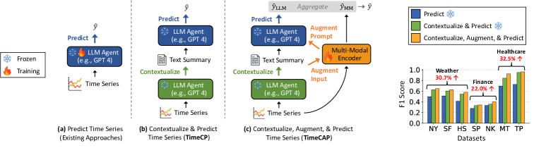
Figure 1: Approaches for time series event prediction using LLMs: (a) Existing methods use LLMs directly as predictors for time series data. (b) Our TimeCP employs two LLM agents: the first agent, $\mathcal{A}_{\text{C}}$, contextualizes time series data into a text summary, and the second agent, $\mathcal{A}_{\text{P}}$, makes predictions based on this summary. (c) Our TimeCAP incorporates a multi-modal encoder that synergizes with LLM agents. The multi-modal encoder generates predictions using both the generated text and the time series data. Additionally, it samples relevant text from the training set to augment the prompt for $\mathcal{A}_{\text{P}}$ to make predictions. TimeCAP achieves a 21.98% improvement in F1 scores using contextualization alone and a 28.75% improvement with the addition of augmentation for time series event predictions on real-world datasets.

Notably, prior approaches leveraging LLMs for making predictions based on time series data have primarily focused on using LLMs as predictors. These methods either fine-tune LLMs or employ soft or hard prompting techniques, as illustrated in Figure 1 (a). This approach often overlooks the importance of contextual understanding in time series analysis, such as the impact of geographical or climatic influences in weather prediction or the interdependencies between economic indicators in financial prediction. By harnessing the domain knowledge and contextual understanding capabilities of LLMs, we can uncover potential insights that can be overlooked by specialized time series models, leading to more comprehensive and accurate predictions.

In light of these insights, we present a novel framework that leverages LLMs not only as predictors but also as a contextualizer of time series data. Our preliminary method, TimeCP (Contextualize & Predict), incorporates two independent LLM agents, as illustrated in Figure 1 (b). The first agent generates a textual summary that provides a comprehensive contextual understanding of the input time series data, drawing on the LLM’s extensive domain knowledge. This summary is then used by the second agent to make more informed predictions of future events. By contextualizing the time series data, TimeCP significantly enhances predictive performance compared to directly prompting LLMs with raw time series data or its parameterized embeddings.

Building upon TimeCP, we introduce TimeCAP (Contextualize, Augment, & Predict), an advanced framework that further leverages text summaries generated by the first LLM agent as augmentations to the time series data. TimeCAP incorporates a multi-modal encoder trained to predict events and learn representations using both the textual summaries and the raw time series data, as illustrated in Figure 1 (c). The representations learned by the multi-modal encoder are then used to select relevant text summaries from the training set, which are provided as in-context examples to augment the prompt for the second LLM agent. This mutual enhancement, wherein the first LLM agent provides the encoder with contextualized information (i.e., input augmentation) and the enriched encoder supplies in-context examples to the second LLM agent (i.e., prompt augmentation), significantly improves overall performance.

Furthermore, TimeCAP is compatible with LLMs accessible through Language Modeling as a Service (LMaaS) (Sun et al. 2022), ensuring broader applicability to black-box APIs (Achiam et al. 2023). Additionally, TimeCAP provides interpretable rationales for its predictions, addressing the critical need for transparency which is often overlooked in recent time series methods involving LLMs.

Our contributions are summarized as follows:

• Novel framework. We introduce TimeCAP, a novel and interpretable framework that leverages two LLM agents (as a contextualizer and a predictor) for event prediction using time series. It is further enhanced by mutual enhancement with a multi-modal encoder.

• Prediction accuracy. Our experimental results demonstrate that TimeCAP outperforms state-of-the-art methods in event prediction by up to 157% in terms of F1 score.

• Data contribution. We collect seven real-world time series datasets from three different domains where underlying contextual understanding is crucial for effective time series modeling. We release these datasets, along with the generated contextual text summaries by the LLM, to support future research and development in this domain.

2 Related Work

Large Language Models. In recent years, language models (LMs) such as BERT (Devlin et al. 2019), RoBERTa (Liu et al. 2019), and DistilBERT (Sanh et al. 2019) have evolved to large language models (LLMs) with multi-billion parameter architectures.  LLMs, including GPT-4 (Achiam et al. 2023), LLaMA-2 (Touvron et al. 2023), and PaLM (Anil et al. 2023), are trained on massive text corpora and have demonstrated impressive performance in various natural language tasks such as translation, summarization, and question answering. These models possess extensive domain knowledge and exhibit zero-shot generalization capability, enabling them to perform tasks without specific training on those tasks (Yang et al. 2024; Brown et al. 2020; Kojima et al. 2022). Additionally, they exhibit emergent abilities such as arithmetic, multi-step reasoning, and instruction following, which LLMs were not explicitly trained for (Wei et al. 2022). Their performance can be further enhanced through in-context learning, where a few input-label pairs are provided as demonstrations (Brown et al. 2020; Min et al. 2022; Liu et al. 2021). Their versatility has enabled adoption across various fields, including computer vision (Koh, Salakhutdinov, and Fried 2023; Guo et al. 2023; Pan et al. 2023; Tsimpoukelli et al. 2021), tabular data analysis (Hegselmann et al. 2023; Narayan et al. 2022), and audio processing (Deshmukh et al. 2024; Tang et al. 2024).

LLMs and Time Series. Recent advancements in LLMs have attracted attention to their integration into time series analysis. Approaches include training LLMs (or LMs) from scratch (Ansari et al. 2024; Nie et al. 2023; Zhang and Yan 2022) or fine-tuning pre-trained LLMs (Zhou et al. 2024; Chang, Peng, and Chen 2023), using time series data. Another approach is prompt tuning, where time series data is parameterized and input into either frozen LLMs (Jin et al. 2024; Sun et al. 2024) or trainable LLMs (Cao et al. 2023). These approaches bridge the gap between time series and LLMs by either integrating LLMs directly with time series data (LLM-for-time series) or aligning time series data with the LLM embedding spaces (time series-for-LLM) (Sun et al. 2024). Some studies use pre-trained LLMs without additional training (i.e., zero-shot prompting) (Gruver et al. 2023; Liu et al. 2023b; Xue and Salim 2023). For example, PromptCast (Xue and Salim 2023) textualizes time series inputs into prompts with basic contextual information. For a more comprehensive overview, refer to recent surveys (Jin et al. 2023; Jiang et al. 2024; Zhang et al. 2024).

Our Work. Existing methods have focused on leveraging LLMs as direct predictors using time series through (fine-) tuning or soft/hard prompting. In this work, we utilize LLMs for two additional purposes beyond their typical role as a predictor. Specifically, LLMs in TimeCAP play a role as a contextualizer of time series data, providing a high-quality augmentation that further enhances prediction performance.

3 Proposed Method

We present our framework for predicting events based on time series using LLMs. We begin with the problem statement. Next, we present TimeCP, our initial method, which utilizes two LLM agents with distinct roles. Then, we describe TimeCAP, our ultimate version. Lastly, we discuss how TimeCAP offers interpretability for its predictions.

3.1 Problem Statement

We formally introduce LLMs and discuss the problem of time series event prediction.

Large Language Models. Let us define an LLM $\mathcal{M}_{\theta}$, parameterized by $\theta$, which is pre-trained on extensive text corpora. We keep $\theta$ fixed (i.e., frozen), employing LLMs in a zero-shot manner without any parameter updates or gradient computations, making them LMaaS-compatible. The LLM takes data of interest $D$ and optional supplementary data $S$ (e.g., demonstrations) to enhance understanding of $D$ and generate a more effective response $R$. Utilizing a prompt generation function $p$, a prompt $p(D,S)$ is constructed, e.g., “Refer to $S$ and predict/summarize $D$.” The inference of the LLM can thus be expressed as $R=\mathcal{M}_{\theta}(p(D,S))$.

In this context, we refer to LLM agents as specialized instances of $\mathcal{M}_{\theta}$ designed to perform specific tasks. Each LLM agent is tailored to leverage its pre-trained domain knowledge to address different aspects of time series event prediction. Their roles are determined by distinct prompt functions, such as predicting or summarizing the given data.

Time Series Event Prediction. Given a time series $\bm{x}=(x_{1},\cdots,x_{L})$, where $L$ is the number of past timesteps and each $x_{t}\in\mathbb{R}^{C}$ represents data from $C$ channels at timestep $t$, the goal of time series event prediction is to predict the outcome $\bm{y}$ of a future event. Real-world time series data (e.g., hourly humidity and temperature) is often associated with contextual information (e.g., geographical or climate factors) derived from domain knowledge. This contextual information is crucial for accurate future event predictions (e.g., forecasting next-day rain). We define the problem as a multi-class classification task and leave the exploration of regression-based event forecasting for future work.

3.2 TimeCP: Contextualize and Predict

We introduce TimeCP, our preliminary method for LLM-based time series event prediction. TimeCP leverages the contextual information associated with time series data to enhance the comprehension and predictive capabilities of LLMs in a zero-shot manner.

PromptCast (Xue and Salim 2023) is a direct counterpart to TimeCP, as it prompts the LLM with a textualized prompt of time series to make predictions. However, it focuses on using LLMs as a predictor and does not fully utilize their contextualization capabilities.

To address this limitation, TimeCP introduces two independent LLM agents, $\mathcal{A}_{\text{C}}$ and $\mathcal{A}_{\text{P}}$, which aim to better leverage the contextualization capabilities of LLMs for time series event prediction. The first agent, $\mathcal{A}_{\text{C}}$, generates a textual summary $\bm{s}_{\bm{x}}$ that contains the underlying context of the given time series $\bm{x}$ by leveraging its domain knowledge:

$$\bm{s}_{\bm{x}}=\mathcal{A}_{\text{C}}(\bm{x})=\mathcal{M}_{\theta}(p_{\text{C}}(\bm{x})),$$

where $p_{\text{C}}(\bm{x})$ is a prompt that instructs the LLM to contextualize $\bm{x}$. The generated summary, $\bm{s}_{\bm{x}}$, includes relevant contextual insights beyond the raw time series data $\bm{x}$, which is then used by the second agent, $\mathcal{A}_{\text{P}}$, to make more informed event predictions:

$$\hat{\bm{y}}_{\text{LLM}}=\mathcal{A}_{\text{P}}(\bm{s}_{\bm{x}})=\mathcal{M}_{\theta}(p_{\text{P}}(\bm{s}_{\bm{x}})),$$

where $p_{\text{P}}(\bm{s}_{\bm{x}})$ is a prompt that instructs the LLM to predict the outcome of the event based on $\bm{s}_{\bm{x}}$. By incorporating the context-informed summary generated by $\mathcal{A}_{\text{C}}$, $\mathcal{A}_{\text{P}}$ can account for the broader context in its predictions. As shown in Figure 1, our dual-agent-based approach consistently outperforms the single-agent approach (spec., PromptCast), which directly predicts the event from the input time series data, i.e., $\mathcal{M}_{\theta}(p_{\text{P}}(\bm{x}))$. The enhanced accuracy demonstrates the effectiveness of generating and utilizing contextual information for future event predictions with LLMs.

3.3 TimeCAP: Contextualize, Augment, Predict

Building upon TimeCP, we present TimeCAP, an advanced version of our framework. TimeCAP trains a multi-modal encoder that synergizes with the LLM agents by introducing dual augmentations (spec., input and prompt augmentations) where the multi-modal encoder and LLM agents complement each other, enabling TimeCAP to make more accurate and reliable event predictions.

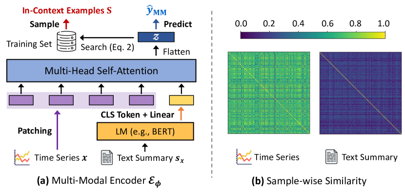
Figure 2: (a) The multi-modal encoder $\mathcal{E}_{\phi}$ generates an embedding $\bm{z}$ and a prediction $\hat{\bm{y}}_{\text{MM}}$ based on the multi-modal input $(\bm{x},\bm{s}_{\bm{x}})$, i.e., time series and its augmented text summary (Eq. (1)). The generated embedding $\bm{z}$ is used to retrieve relevant summaries from the training set to serve as in-context examples to augment the prompt for $\mathcal{A}_{\text{P}}$ (Eq. (2)). (b) The similarity patterns within the time series and the text vary; time series similarities are generally high, while text similarities are selectively highlighted, implying complementary information in each modality.

Multi-Modal Encoder. We introduce a trainable encoder $\mathcal{E}_{\phi}$, parameterized by $\phi$ (Figure 3 (a)). This encoder aims to capture intricate dynamic patterns in time series data more effectively than zero-shot LLMs. In addition to time series $\bm{x}$, it incorporates the textual summary $\bm{s}_{\bm{x}}$ generated by $\mathcal{A}_{\text{C}}$, which provides additional contextual insights beyond the raw time series data (i.e., input augmentation), as shown in Figure 3 (b). The encoder $\mathcal{E}_{\phi}$ generates its prediction $\hat{\bm{y}}_{\text{MM}}$ and the embedding $\bm{z}$ of the multi-modal input $(\bm{x},\bm{s}_{\bm{x}})$ as:

$$(\hat{\bm{y}}_{\text{MM}},\;\bm{z})=\mathcal{E}_{\phi}(\bm{x},\bm{s}_{\bm{x}}),$$ (1)

where $\bm{z}$ is used for sampling in-context examples (Eq. (2)). The encoder consists of (1) a language model that embeds text into the latent space and (2) a transformer encoder that captures dependencies between the two modalities.

The corresponding text summary $\bm{s}_{\bm{x}}$ is processed by a pre-trained language model (LM) with substantially fewer parameters, which is thus relatively easier to fine-tune. Specifically, we represent $\bm{s}_{\bm{x}}$ using the LM as $\hat{\bm{z}}=\mathtt{LM}(\bm{s}_{\bm{x}})\in\mathbb{R}^{d^{\prime}}$, leveraging the output CLS token embedding. This representation is then projected as $\tilde{\bm{z}}_{\text{text}}=\hat{\bm{z}}\mathbf{W}_{\text{text}}\in\mathbb{R}^{d}$ using a linear layer $\mathbf{W}_{\text{text}}\in\mathbb{R}^{d^{\prime}\times d}$.

For time series, motivated by the effectiveness of patching (Nie et al. 2023; Zhang and Yan 2022), we segment a time series $\bm{x}^{(i)}\in\bm{x}$ of the $i$^th channel into $N$ non-overlapping patches $\hat{\bm{x}}^{(i)}\in\mathbb{R}^{N\times L_{p}}$ with patch length $L_{p}$ and stride $L_{s}$, where $N=\lceil\frac{L-L_{p}}{L_{s}}\rceil+1$ holds. These patches are then projected as $\tilde{\bm{z}}_{\text{time}}^{(i)}=\hat{\bm{x}}^{(i)}\mathbf{W}_{\text{time}}\in\mathbb{R}^{N\times d}$ using a simple linear layer $\mathbf{W}_{\text{time}}\in\mathbb{R}^{L_{p}\times d}$.

For each $i$^th channel of the time series, we concatenate the time series patch embeddings $\tilde{\bm{z}}_{\text{time}}^{(i)}$ and the text embedding $\tilde{\bm{z}}_{\text{text}}$ to construct $\tilde{\bm{z}}^{(i)}=[\tilde{\bm{z}}_{\text{time}}^{(i)};\tilde{\bm{z}}_{\text{text}}]\in\mathbb{R}^{(N+1)\times d}$. We then use multi-head self-attention to capture the relationships between this combined representation. More specifically, for each attention head $h\in\{1,\cdots,H\}$, we compute query $\mathbf{Q}_{h}^{(i)}=\tilde{\bm{z}}^{(i)}\mathbf{W}_{h}^{Q}$, key $\mathbf{K}_{h}^{(i)}=\tilde{\bm{z}}^{(i)}\mathbf{W}_{h}^{K}$, and value $\mathbf{V}_{h}^{(i)}=\tilde{\bm{z}}^{(i)}\mathbf{W}_{h}^{V}$ matrices using $\mathbf{W}_{h}^{Q},\mathbf{W}_{h}^{K},\mathbf{W}_{h}^{V}\in\mathbb{R}^{d\times d/H}$. Each $h$^th attention head is then defined as:

The outputs of the attention heads are aggregated and projected as $\bm{z}^{(i)}=[\bm{z}_{1}^{(i)};\cdots;\bm{z}_{H}^{(i)}]\mathbf{W}^{H}\in\mathbb{R}^{d}$ where $\mathbf{W}^{H}\in\mathbb{R}^{d\times d}$. Then, a flatten layer represents all channels as a single embedding vector, i.e., $\bm{z}=[\bm{z}^{(1)};\cdots;\bm{z}^{(C)}]\in\mathbb{R}^{dC}$. Finally, a linear layer $\mathbf{W}^{P}\in\mathbb{R}^{dC\times K}$ is applied to $\bm{z}$ to obtain a $K$-dimensional prediction logit, i.e,. $\hat{\bm{y}}_{\text{MM}}=\bm{z}\mathbf{W}^{P}\in\mathbb{R}^{K}$. We fine-tune the parameters $\phi$ including those of the LM and the transformer encoder using cross-entropy loss.

Domain	Dataset	Resolution	# Channels	# Timestamps	# Samples	Duration	Label Distribution
Weather	New York (NY)	Hourly	5	45,216	1,884	2012.10 - 2017.11	Rain (24.26%) / Not rain (75.74%)
	San Francisco (SF)	Hourly	5	45,216	1,884	2012.10 - 2017.11	Rain (24.58%) / Not rain (75.42%)
	Houston (HS)	Hourly	5	45,216	1,884	2012.10 - 2017.11	Rain (30.94%) / Not rain (69.06%)
Finance	S&P 500 (SP)	Daily	9	1,258	1,238	2019.01 - 2023.12	Inc. (13.78%) / Dec. (17.04%) / Etc. (69.18%)
	Nikkei 225 (NK)	Daily	9	1,258	1,238	2019.01 - 2023.12	Inc. (15.02%) / Dec. (17.12%) / Etc. (67.86%)
Healthcare	Mortality (MT)	Weekly	4	395	375	2016.07 - 2024.06	Exceed (69.33%) / Not exceed (30.67%)
	Test-Positive (TP)	Weekly	6	447	427	2015.10 - 2024.04	Exceed (65.77%) / Not exceed (34.23%)

Table 1: Statistics of seven real-world datasets for time series event prediction. These publicly available datasets are expected to benefit from contextual understanding beyond raw time series data. More details can be found in the supplementary document.

In-Context Example Sampling. Once the multi-modal encoder is trained, it aids $\mathcal{A}_{\text{P}}$ in making more informed predictions by sampling relevant text summaries from the training set as valuable demonstrations (i.e., prompt augmentation).

Given the embedding $\bm{z}$ of the multi-modal input ($\bm{x}$, $\bm{s}_{\bm{x}}$), we retrieve $k$ summaries from the training set whose embeddings are closest to $\bm{z}$. Formally, let $\mathcal{T}$ denote the training set, and $\bm{\mathcal{Z}}\in\mathbb{R}^{|\mathcal{T}|\times dC}$ represent the set of embeddings of the training samples generated by $\mathcal{E}_{\phi}$. The $k$ pairs of text summaries and their corresponding outcomes are retrieved as the nearest neighbors of $\bm{z}$ in the embedding space, as follows:

$$\mathbf{S}=\{(\bm{s}_{\bm{x}_{j}},\bm{y}_{j}):j\in\text{NN}_{k}(\bm{z})\},$$ (2)

where $$\text{NN}_{k}(\bm{z})={\text{arg}\;\text{top-}{k}}_{j\in\mathcal{T}}(-\|\bm{z}-\bm{\mathcal{Z}}_{j}\|).$$

These summaries and their outcomes are used as in-context examples for $\mathcal{A}_{\text{P}}$ to predict the outcome of $\bm{s}_{\bm{x}}$ as follows:

$$\hat{\bm{y}}_{\text{LLM}}=\mathcal{A}_{\text{P}}\left(\bm{s}_{\bm{x}},\mathbf{S}\right)=\mathcal{M}_{\theta}\left(p_{\text{P}}(\bm{s}_{\bm{x}},\mathbf{S})\right).$$ (3)

These examples help the agent $\mathcal{A}_{\text{P}}$ better understand the test input by comparing the summaries and reasoning based on them. This leads to more accurate predictions, as shown in Figure 1 and further validated in Section 4.

Fused Prediction. Lastly, we integrate the predictions from the multi-modal encoder (Eq. (1)) and $\mathcal{A}_{\text{P}}$ (Eq. (3)) through a linear combination, i.e., $\hat{\bm{y}}=\lambda\hat{\bm{y}}_{\text{LLM}}+(1-\lambda)\hat{\bm{y}}_{\text{MM}}$ where $\lambda\in[0,1]$ is a hyperparameter. Given that the prediction $\hat{\bm{y}}_{\text{LMM}}$ produced by $\mathcal{A}_{\text{P}}$ is discrete, we convert it into a one-hot vector to enable its fusion with the continuous logit $\hat{\bm{y}}_{\text{MM}}$. This fusion leverages complementary information from both models, enhancing the overall performance of TimeCAP, as demonstrated in Section 4.

3.4 Interpreting the Predictions

We explore how TimeCAP provides interpretations for its predictions by introducing two variants of the prompt function $p_{\text{P}}$ used in $\mathcal{A}_{\text{P}}$. The resulting variants, $\mathcal{A}_{\text{P}}^{\text{I}}$ and $\mathcal{A}_{\text{P}}^{\text{E}}$, enable distinct interpretations, enhancing transparency.

Implicit Interpretation. We prompt the LLM $\mathcal{M}_{\theta}$ to generate both a prediction and its corresponding rationale:

$$(\hat{\bm{y}}_{\text{LLM}},\;\bm{r})=\mathcal{A}_{\text{P}}^{\text{I}}(\bm{s}_{\bm{x}},\mathbf{S})=\mathcal{M}_{\theta}\left(p_{\text{P}}^{\text{I}}(\bm{s}_{\bm{x}},\mathbf{S})\right),$$

where $p_{\text{P}}^{\text{I}}$ is a prompt function that instructs $\mathcal{M}_{\theta}$ to predict the event ($\hat{\bm{y}}_{\text{LLM}}$) and also provide the rationale ($\bm{r}$) behind its prediction. This rationale leverages the LLM’s domain knowledge and reasoning capabilities. While the in-context examples $\mathbf{S}$ are optional, as shown in Section 4, their inclusion leads to distinct implicit interpretations.

Explicit Interpretation. We prompt $\mathcal{M}_{\theta}$ to identify the most useful or relevant example from the in-context set $\mathbf{S}$:

$$(\hat{\bm{y}}_{\text{LLM}},\;\bm{s}_{\bm{x}_{j^{*}}})=\mathcal{A}_{\text{P}}^{\text{E}}(\bm{s}_{\bm{x}},\mathbf{S})=\mathcal{M}_{\theta}\left(p_{\text{P}}^{\text{E}}(\bm{s}_{\bm{x}},\mathbf{S})\right),$$

where $p_{\text{P}}^{\text{E}}$ is a prompt function that instructs $\mathcal{M}_{\theta}$ to predict the event ($\hat{\bm{y}}_{\text{LLM}}$) and select the most relevant example ($\bm{s}_{\bm{x}_{j^{*}}}$) from $\mathbf{S}$. In addition, the input time series $\bm{x}$ can be compared with the corresponding time series $\bm{x}_{j^{*}}$ for further analyses.

4 Experiments

In this section, we present TimeCAP’s: (1) accuracy compared with the state-of-the-art methods, (2) component effectiveness, (3) interpretability, and (4) additional analyses.

4.1 Experimental Settings

We first report the experimental settings. We use GPT-4 (Achiam et al. 2023) as the default backbone for the LLM agents and BERT (Devlin et al. 2019) as the LM within the multi-modal encoder. We describe the prompt functions in the supplementary document.

	Weather						Finance				Healthcare
Datasets $\rightarrow$	New York		San Fran.		Houston		S&P 500		Nikkei 225		Mortality		Test-Positive		Avg. Rank
Methods $\downarrow$	F1	AUC	F1	AUC	F1	AUC	F1	AUC	F1	AUC	F1	AUC	F1	AUC	F1	AUC
Autoformer (Wu et al. 2021)	0.546	0.590	0.475	0.539	0.542	0.592	0.330	0.471	0.358	0.568	0.683	0.825	0.774	0.918	9.14	10.00
Crossformer (Zhang and Yan 2022)	0.500	0.594	0.546	0.594	0.611	0.672	0.330	0.561	0.283	0.610	0.737	0.914	0.924	0.984	6.86	5.14
TimesNet (Wu et al. 2022)	0.494	0.594	0.521	0.557	0.614	0.663	0.288	0.566	0.272	0.473	0.558	0.903	0.794	0.867	9.57	8.57
DLinear (Zeng et al. 2023)	0.540	0.660	0.553	0.633	0.592	0.669	0.174	0.463	0.278	0.509	0.419	0.388	0.393	0.500	10.43	9.43
TSMixer (Chen et al. 2023)	0.488	0.534	0.577	0.577	0.522	0.589	0.405	0.567	0.367	0.516	0.808	0.931	0.550	0.600	7.43	9.00
PatchTST (Nie et al. 2023)	0.592	0.675	0.542	0.565	0.593	0.652	0.373	0.573	0.391	0.640	0.695	0.928	0.841	0.934	5.14	5.00
FreTS (Yi et al. 2024)	0.625	0.689	0.504	0.533	0.592	0.673	0.351	0.532	0.381	0.575	0.464	0.500	0.817	0.812	6.86	8.00
iTransformer (Liu et al. 2024)	0.541	0.650	0.534	0.566	0.569	0.655	0.285	0.537	0.269	0.462	0.797	0.972	0.887	0.950	8.71	7.29
LLMTime (Kojima et al. 2022) ✻	0.587	0.657	0.542	0.563	0.587	0.626	0.306	0.492	0.166	0.510	0.769	0.804	0.802	0.817	8.43	9.86
PromptCast (Xue and Salim 2023) ✻	0.499	0.365	0.510	0.397	0.412	0.400	0.276	0.488	0.333	0.517	0.695	0.869	0.727	0.768	11.00	12.00
GPT4TS (Zhou et al. 2024)	0.501	0.606	0.550	0.612	0.612	0.692	0.285	0.414	0.297	0.531	0.901	0.992	0.774	0.879	7.00	6.14
Time-LLM (Jin et al. 2024)	0.613	0.699	0.577	0.593	0.592	0.625	0.357	0.552	0.294	0.526	0.659	0.926	0.671	0.864	7.00	6.86
TimeCP ✻	0.625	0.706	0.603	0.607	0.544	0.593	0.330	0.510	0.364	0.532	0.842	0.946	0.949	0.956	4.43	5.57
TimeCAP	0.676	0.745	0.632	0.676	0.614	0.675	0.398	0.546	0.428	0.640	0.947	1.000	0.962	0.995	1.14	1.86

Table 2: The F1 score (F1) and the AUROC (AUC) for TimeCP, TimeCAP, and their competitors on seven real-world time series datasets. TimeCAP outperforms other methods on most datasets and ranks first on average. Methods annotated with ^✻ make predictions in a zero-shot manner. The best and second-best scores are highlighted in bold and underline, respectively.

Datasets and Tasks. We collected seven real-world time series datasets from three domains: weather, finance, and healthcare, for time series event prediction, as summarized in Table 1. Note that only time series data is provided, and the text data is generated by $\mathcal{A}_{\text{C}}$. Below, we describe the datasets and their respective tasks in each domain.

• Weather: Datasets in this domain consist of hourly time series data on temperature, humidity, air pressure, wind speed, and wind direction in New York (NY), San Francisco (SF), and Houston (HS). Given the last 24 hours of time series data, the task is to predict the event of whether it will rain in the next 24 hours.

• Finance: Datasets in this domain contain daily time series data for nine financial indicators (e.g., S&P 500, VIX, and exchange rates). The task is to predict whether the price of S&P 500 (SP) or Nikkei 225 (NK) will (1) increase by more than 1%, (2) decrease by more than 1%, or (3) otherwise remain relatively stable.

• Healthcare: The mortality (MT) dataset includes weekly data including influenza and pneumonia deaths, and the task is to predict if the mortality ratio from influenza/pneumonia will exceed the average threshold. The test-positive (TP) dataset includes weekly data including the number of positive specimens for Influenza A & B, and the task is to predict if the ratio of respiratory specimens testing positive for influenza will exceed the average threshold.

We release the datasets with their text summaries generated by $\mathcal{A}_{\text{C}}$. See the supplementary document for more details.

Baselines. We consider state-of-the-art time series prediction models, including Autoformer (Wu et al. 2021), Crossformer (Zhang and Yan 2022), TimesNet (Wu et al. 2022), DLinear (Zeng et al. 2023), PatchTST (Nie et al. 2023), FreTS (Yi et al. 2024), and iTransformer (Liu et al. 2024) as well as recent LLM-based models, including LLMTime (Kojima et al. 2022), PromptCast (Xue and Salim 2023), GPT4TS (Zhou et al. 2024), and Time-LLM (Jin et al. 2024), as baselines. While these methods are primarily designed for regression-based time series prediction, they can be easily adapted for event prediction (i.e., classification) tasks.  See the supplementary document for more details.

Evaluation. We evaluate TimeCAP and its competitors on time series event prediction using the F1 Score and AUROC. We split data into training, validation, and test sets in a 6:2:2 ratio and set $k=5$, unless otherwise stated. We run five times for each setting. For other hyperparameter settings, refer to the supplementary document.

4.2 Accuracy

We first report the predictive performance of TimeCAP and its competitors on time series event prediction.

Main Results. Table 2 presents the performance of TimeCAP, TimeCP, and their competitors across all datasets. TimeCAP achieves the best average performance and overall ranks. These results demonstrate the effectiveness of our framework in contextualizing time series data and the mutual enhancement with the multi-modal encoder.

Zero-shot Results. TimeCP predicts events in a zero-shot manner without referencing other training samples. As shown in Table 2, TimeCP significantly outperforms other zero-shot LLM-based methods (LLMTime (Kojima et al. 2022) and PromptCast (Xue and Salim 2023)) across all datasets. While competitors use LLMs mainly as predictors, TimeCP leverages LLMs’ domain knowledge and reasoning capabilities to understand the context of the time series, which leads to more accurate predictions.

		Weather			Finance		Healthcare		Avg.
		NY	SF	HS	SP	NK	MT	TP	Rank
(1) Context	PromptCast	0.499	0.510	0.412	0.276	0.333	0.695	0.727	8.86
	TimeCP	0.625	0.603	0.544	0.330	0.364	0.842	0.949	5.57
(2) Input	Only Time	0.592	0.542	0.593	0.373	0.391	0.695	0.841	6.43
	Time+Text	0.623	0.576	0.606	0.398	0.428	0.734	0.937	4.29
(3) Prompt	Random	0.619	0.621	0.528	0.322	0.344	0.901	0.883	6.57
	Only Time	0.625	0.599	0.571	0.305	0.379	0.947	0.948	5.14
	Time+Text	0.641	0.626	0.578	0.341	0.401	0.947	0.961	3.00
(4) Fusion	Select-One	0.641	0.626	0.606	0.398	0.428	0.947	0.961	1.57
	Aggregate	0.676	0.632	0.614	0.398	0.428	0.947	0.962	1.00

Table 3: Ablation studies of TimeCAP. Every component of TimeCAP contributes to the improvement of the predictive performance in terms of the F1 score.

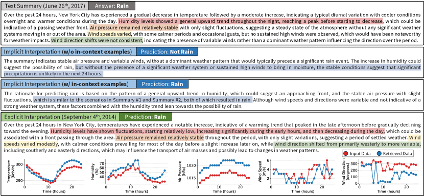
Figure 3: A case study on interpretations of TimeCAP. Given a text summary: (a) implicit interpretations depend on the presence of in-context examples (blue), and (b) explicit interpretations involve post-hoc comparisons between the input and a selected in-context example with similar semantics (red, orange, yellow, and green).

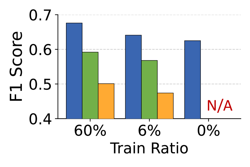
(a) Weather (NY)

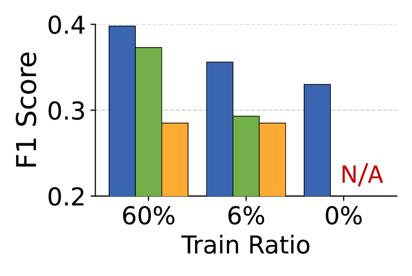
(b) Finance (SP)

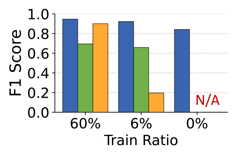
(c) Healthcare (MT)

Figure 4: TimeCAP consistently outperforms its competitors (spec., PatchTST and GPT4TS) across different training ratios. When the training ratio is 0%, TimeCP is used.

4.3 Effectiveness

We verify the effectiveness of each component of TimeCAP through ablation studies as summarized in Table 3.

Contextualization. As shown in (1) in Table 3, TimeCP consistently and significantly outperforms PromptCast, which directly prompts LLMs to predict the future event, across all datasets. This demonstrates the effectiveness TimeCP’s dual-agent approach in contextualizing time series data for event prediction.

Augmentation. TimeCAP incorporates dual augmentations: $\mathcal{A}_{\text{C}}$ generates textual summaries to augment the time series data (i.e., input augmentation), and the multi-modal encoder samples in-context examples to augment prompts for $\mathcal{A}_{\text{P}}$ (i.e., prompt augmentation). We evaluate the effectiveness of each augmentation.

• Input Augmentation. Our multi-modal encoder, which incorporates both time series and text data, consistently outperforms its variant that relies only on time series data, as shown in (2) of Table 3. This demonstrates that the textual summaries generated by $\mathcal{A}_{\text{C}}$ provide complementary information that enhances the predictive performance.

• Prompt Augmentation. We compare the performance of TimeCAP using different in-context sampling strategies. As shown in (3) of Table 3, examples selected by our multi-modal encoder, which leverages both time series and text data, provide more meaningful demonstrations, as evidenced by its superior performance compared to random sampling and the time series-only encoder.

Prediction Fusion. The final prediction of TimeCAP is obtained by aggregating the predictions from the multi-modal encoder $\mathcal{E}_{\phi}$ and the LLM agent $\mathcal{A}_{\text{P}}$. As shown in (4) of Table 3, this combined approach generally enhances overall performance, often exceeding the best performance of each model independently (i.e., select-one). This indicates that the predictions from the two models are complementary, leveraging each other’s strengths.

4.4 Interpretability

We evaluate the interpretation provided by TimeCAP (see Section 3.4) through a case study, as illustrated in Figure 3.

Implicit Interpretation. The presence of in-context examples significantly affects interpretation and prediction. Without in-context examples, the LLM predicts the outcome solely based on the input data, which can result in incorrect predictions. In contrast, with in-context examples, the LLM leverages past text-outcome relationships, leading to more informed predictions and interpretations.

Explicit Interpretation. The LLM agent selects a text summary from the provided in-context examples that align with the input text. The selected in-context examples serve as valuable references for post-hoc interpretation of the prediction. Moreover, the corresponding time series can be compared with the input time series for further interpretation.

4.5 Further Analyses

We provide additional experimental results with TimeCAP.

Few-Data Results. We evaluate TimeCAP and two leading competitors, PatchTST and GPT4TS, on a reduced training set, specifically reducing it to 10% of the default training ratio and even to 0%. As shown in Figure 4, while the competitors suffer from data scarcity, TimeCAP relatively maintains its performance with the reduced training size. Furthermore, it achieves high zero-shot performance, which demonstrates the effectiveness of TimeCAP in data-scarce scenarios, which is valuable for real-world applications.

Classifier	In-Context Sampler	Weather	Finance	Healthcare
KNN	PatchTST	0.540	0.325	0.657
	MM Encoder	0.555	0.338	0.736
LLM ($\mathcal{A}_{\text{P}}$)	None (Zero-shot)	0.591	0.347	0.896
	PatchTST	0.598	0.342	0.948
	MM Encoder	0.615	0.371	0.954

Table 4: Our multi-modal (MM) encoder selects more useful in-context examples than PatchTST, as indicated by higher average F1 scores in each domain, enabling $\mathcal{A}_{\text{P}}$ to make more accurate event predictions.

Quality of In-Context Examples. We evaluate the quality of in-context examples selected by our multi-modal encoder compared to those chosen by PatchTST using a KNN classifier, which predicts the class of the input based on the majority labels of the $k$ in-context examples. As shown in Table 4, the KNN with our multi-modal encoder outperforms that with PatchTST, indicating that our encoder generates embeddings that are more useful as in-context examples. Consequently, this leads to more accurate predictions by $\mathcal{A}_{\text{P}}$ when used as in-context examples.

5 Conclusion

In this work, we introduce TimeCAP, a novel framework that leverages LLM’s contextual understanding for time series event prediction. TimeCAP employs two independent LLM agents for contextualization and prediction, supported by a trainable multi-modal encoder that mutually enhances them. Our experimental results on seven real-world time series datasets from various domains demonstrate the effectiveness of TimeCAP.

References

- Achiam et al. (2023) Achiam, J.; Adler, S.; Agarwal, S.; Ahmad, L.; Akkaya, I.; Aleman, F. L.; Almeida, D.; Altenschmidt, J.; Altman, S.; Anadkat, S.; et al. 2023. Gpt-4 technical report. arXiv preprint arXiv:2303.08774.
- Anil et al. (2023) Anil, R.; Dai, A. M.; Firat, O.; Johnson, M.; Lepikhin, D.; Passos, A.; Shakeri, S.; Taropa, E.; Bailey, P.; Chen, Z.; et al. 2023. Palm 2 technical report. arXiv preprint arXiv:2305.10403.
- Ansari et al. (2024) Ansari, A. F.; Stella, L.; Turkmen, C.; Zhang, X.; Mercado, P.; Shen, H.; Shchur, O.; Rangapuram, S. S.; Arango, S. P.; Kapoor, S.; et al. 2024. Chronos: Learning the language of time series. arXiv preprint arXiv:2403.07815.
- Berndt and Clifford (1994) Berndt, D. J.; and Clifford, J. 1994. Using dynamic time warping to find patterns in time series. In KDD.
- Brown et al. (2020) Brown, T.; Mann, B.; Ryder, N.; Subbiah, M.; Kaplan, J. D.; Dhariwal, P.; Neelakantan, A.; Shyam, P.; Sastry, G.; Askell, A.; et al. 2020. Language models are few-shot learners. In NeurIPS.
- Cao et al. (2023) Cao, D.; Jia, F.; Arik, S. O.; Pfister, T.; Zheng, Y.; Ye, W.; and Liu, Y. 2023. TEMPO: Prompt-based Generative Pre-trained Transformer for Time Series Forecasting. In ICLR.
- Chang, Peng, and Chen (2023) Chang, C.; Peng, W.-C.; and Chen, T.-F. 2023. Llm4ts: Two-stage fine-tuning for time-series forecasting with pre-trained llms. arXiv preprint arXiv:2308.08469.
- Chen et al. (2023) Chen, S.-A.; Li, C.-L.; Arik, S. O.; Yoder, N. C.; and Pfister, T. 2023. TSMixer: An All-MLP Architecture for Time Series Forecasting. Transactions on Machine Learning Research.
- Chowdhury (2010) Chowdhury, G. G. 2010. Introduction to modern information retrieval. Facet publishing.
- Chu et al. (2023) Chu, Z.; Hao, H.; Ouyang, X.; Wang, S.; Wang, Y.; Shen, Y.; Gu, J.; Cui, Q.; Li, L.; Xue, S.; et al. 2023. Leveraging large language models for pre-trained recommender systems. arXiv preprint arXiv:2308.10837.
- Deshmukh et al. (2024) Deshmukh, S.; Elizalde, B.; Emmanouilidou, D.; Raj, B.; Singh, R.; and Wang, H. 2024. Training audio captioning models without audio. In ICASSP.
- Devlin et al. (2019) Devlin, J.; Chang, M.-W.; Lee, K.; and Toutanova, K. 2019. BERT: Pre-training of Deep Bidirectional Transformers for Language Understanding. In NAACL.
- Fathullah et al. (2024) Fathullah, Y.; Wu, C.; Lakomkin, E.; Jia, J.; Shangguan, Y.; Li, K.; Guo, J.; Xiong, W.; Mahadeokar, J.; Kalinli, O.; et al. 2024. Prompting large language models with speech recognition abilities. In ICASSP.
- Gruver et al. (2023) Gruver, N.; Finzi, M.; Qiu, S.; and Wilson, A. G. 2023. Large language models are zero-shot time series forecasters. In NeurIPS.
- Guo et al. (2023) Guo, J.; Li, J.; Li, D.; Tiong, A. M. H.; Li, B.; Tao, D.; and Hoi, S. 2023. From images to textual prompts: Zero-shot visual question answering with frozen large language models. In CVPR.
- Hegselmann et al. (2023) Hegselmann, S.; Buendia, A.; Lang, H.; Agrawal, M.; Jiang, X.; and Sontag, D. 2023. Tabllm: Few-shot classification of tabular data with large language models. In AISTATS.
- Jiang et al. (2024) Jiang, Y.; Pan, Z.; Zhang, X.; Garg, S.; Schneider, A.; Nevmyvaka, Y.; and Song, D. 2024. Empowering Time Series Analysis with Large Language Models: A Survey. arXiv preprint arXiv:2402.03182.
- Jin et al. (2024) Jin, M.; Wang, S.; Ma, L.; Chu, Z.; Zhang, J. Y.; Shi, X.; Chen, P.-Y.; Liang, Y.; Li, Y.-F.; Pan, S.; et al. 2024. Time-LLM: Time Series Forecasting by Reprogramming Large Language Models. In ICLR.
- Jin et al. (2023) Jin, M.; Wen, Q.; Liang, Y.; Zhang, C.; Xue, S.; Wang, X.; Zhang, J.; Wang, Y.; Chen, H.; Li, X.; et al. 2023. Large models for time series and spatio-temporal data: A survey and outlook. arXiv preprint arXiv:2310.10196.
- Kamalloo et al. (2023) Kamalloo, E.; Dziri, N.; Clarke, C.; and Rafiei, D. 2023. Evaluating Open-Domain Question Answering in the Era of Large Language Models. In ACL.
- Koh, Salakhutdinov, and Fried (2023) Koh, J. Y.; Salakhutdinov, R.; and Fried, D. 2023. Grounding language models to images for multimodal inputs and outputs. In ICML.
- Kojima et al. (2022) Kojima, T.; Gu, S. S.; Reid, M.; Matsuo, Y.; and Iwasawa, Y. 2022. Large language models are zero-shot reasoners. In NeurIPS.
- Liévin et al. (2024) Liévin, V.; Hother, C. E.; Motzfeldt, A. G.; and Winther, O. 2024. Can large language models reason about medical questions? Patterns, 5(3): 100943.
- Liu et al. (2023a) Liu, H.; Ma, Z.; Yang, L.; Zhou, T.; Xia, R.; Wang, Y.; Wen, Q.; and Sun, L. 2023a. Sadi: A self-adaptive decomposed interpretable framework for electric load forecasting under extreme events. In ICASSP.
- Liu et al. (2021) Liu, J.; Shen, D.; Zhang, Y.; Dolan, B.; Carin, L.; and Chen, W. 2021. What Makes Good In-Context Examples for GPT-? arXiv preprint arXiv:2101.06804.
- Liu et al. (2023b) Liu, X.; McDuff, D.; Kovacs, G.; Galatzer-Levy, I.; Sunshine, J.; Zhan, J.; Poh, M.-Z.; Liao, S.; Di Achille, P.; and Patel, S. 2023b. Large language models are few-shot health learners. arXiv preprint arXiv:2305.15525.
- Liu et al. (2024) Liu, Y.; Hu, T.; Zhang, H.; Wu, H.; Wang, S.; Ma, L.; and Long, M. 2024. iTransformer: Inverted Transformers Are Effective for Time Series Forecasting. In ICLR.
- Liu et al. (2019) Liu, Y.; Ott, M.; Goyal, N.; Du, J.; Joshi, M.; Chen, D.; Levy, O.; Lewis, M.; Zettlemoyer, L.; and Stoyanov, V. 2019. Roberta: A robustly optimized bert pretraining approach. arXiv preprint arXiv:1907.11692.
- Min et al. (2022) Min, S.; Lyu, X.; Holtzman, A.; Artetxe, M.; Lewis, M.; Hajishirzi, H.; and Zettlemoyer, L. 2022. Rethinking the Role of Demonstrations: What Makes In-Context Learning Work? In EMNLP.
- Mirchandani et al. (2023) Mirchandani, S.; Xia, F.; Florence, P.; Ichter, B.; Driess, D.; Arenas, M. G.; Rao, K.; Sadigh, D.; and Zeng, A. 2023. Large Language Models as General Pattern Machines. In CoRL.
- Narayan et al. (2022) Narayan, A.; Chami, I.; Orr, L.; and Ré, C. 2022. Can Foundation Models Wrangle Your Data? PVLDB, 16(4): 738–746.
- Nie et al. (2023) Nie, Y.; Nguyen, N. H.; Sinthong, P.; and Kalagnanam, J. 2023. A Time Series is Worth 64 Words: Long-term Forecasting with Transformers. In ICLR.
- Pan et al. (2023) Pan, J.; Lin, Z.; Ge, Y.; Zhu, X.; Zhang, R.; Wang, Y.; Qiao, Y.; and Li, H. 2023. Retrieving-to-answer: Zero-shot video question answering with frozen large language models. In ICCV.
- Qin et al. (2023) Qin, C.; Zhang, A.; Zhang, Z.; Chen, J.; Yasunaga, M.; and Yang, D. 2023. Is ChatGPT a General-Purpose Natural Language Processing Task Solver? In EMNLP.
- Sanh et al. (2019) Sanh, V.; Debut, L.; Chaumond, J.; and Wolf, T. 2019. DistilBERT, a distilled version of BERT: smaller, faster, cheaper and lighter. arXiv preprint arXiv:1910.01108.
- Sawhney et al. (2020) Sawhney, R.; Agarwal, S.; Wadhwa, A.; and Shah, R. 2020. Deep attentive learning for stock movement prediction from social media text and company correlations. In EMNLP.
- Schneider and Dickinson (1974) Schneider, S. H.; and Dickinson, R. E. 1974. Climate modeling. Reviews of Geophysics, 12(3): 447–493.
- Shi et al. (2023) Shi, W.; Min, S.; Yasunaga, M.; Seo, M.; James, R.; Lewis, M.; Zettlemoyer, L.; and Yih, W.-t. 2023. Replug: Retrieval-augmented black-box language models. arXiv preprint arXiv:2301.12652.
- Sun et al. (2024) Sun, C.; Li, Y.; Li, H.; and Hong, S. 2024. TEST: Text prototype aligned embedding to activate LLM’s ability for time series. In ICLR.
- Sun et al. (2022) Sun, T.; Shao, Y.; Qian, H.; Huang, X.; and Qiu, X. 2022. Black-box tuning for language-model-as-a-service. In ICML.
- Tang et al. (2024) Tang, C.; Yu, W.; Sun, G.; Chen, X.; Tan, T.; Li, W.; Lu, L.; Ma, Z.; and Zhang, C. 2024. Extending Large Language Models for Speech and Audio Captioning. In ICASSP.
- Team et al. (2023) Team, G.; Anil, R.; Borgeaud, S.; Wu, Y.; Alayrac, J.-B.; Yu, J.; Soricut, R.; Schalkwyk, J.; Dai, A. M.; Hauth, A.; et al. 2023. Gemini: a family of highly capable multimodal models. arXiv preprint arXiv:2312.11805.
- Touvron et al. (2023) Touvron, H.; Martin, L.; Stone, K.; Albert, P.; Almahairi, A.; Babaei, Y.; Bashlykov, N.; Batra, S.; Bhargava, P.; Bhosale, S.; et al. 2023. Llama 2: Open foundation and fine-tuned chat models. arXiv preprint arXiv:2307.09288.
- Tsimpoukelli et al. (2021) Tsimpoukelli, M.; Menick, J. L.; Cabi, S.; Eslami, S.; Vinyals, O.; and Hill, F. 2021. Multimodal few-shot learning with frozen language models. In NeurIPS.
- Wang et al. (2023a) Wang, L.; Lyu, C.; Ji, T.; Zhang, Z.; Yu, D.; Shi, S.; and Tu, Z. 2023a. Document-Level Machine Translation with Large Language Models. In EMNLP.
- Wang et al. (2023b) Wang, Y.; Chu, Z.; Ouyang, X.; Wang, S.; Hao, H.; Shen, Y.; Gu, J.; Xue, S.; Zhang, J. Y.; Cui, Q.; et al. 2023b. Enhancing recommender systems with large language model reasoning graphs. arXiv preprint arXiv:2308.10835.
- Wei et al. (2022) Wei, J.; Tay, Y.; Bommasani, R.; Raffel, C.; Zoph, B.; Borgeaud, S.; Yogatama, D.; Bosma, M.; Zhou, D.; Metzler, D.; et al. 2022. Emergent abilities of large language models. TMLR.
- Wu et al. (2022) Wu, H.; Hu, T.; Liu, Y.; Zhou, H.; Wang, J.; and Long, M. 2022. Timesnet: Temporal 2d-variation modeling for general time series analysis. In ICLR.
- Wu et al. (2021) Wu, H.; Xu, J.; Wang, J.; and Long, M. 2021. Autoformer: Decomposition transformers with auto-correlation for long-term series forecasting. In NeurIPS.
- Xue and Salim (2023) Xue, H.; and Salim, F. D. 2023. Promptcast: A new prompt-based learning paradigm for time series forecasting. TKDE, 36(11): 6851–6864.
- Yang et al. (2024) Yang, J.; Jin, H.; Tang, R.; Han, X.; Feng, Q.; Jiang, H.; Zhong, S.; Yin, B.; and Hu, X. 2024. Harnessing the power of llms in practice: A survey on chatgpt and beyond. TKDD, 18(6): 1–32.
- Yi et al. (2024) Yi, K.; Zhang, Q.; Fan, W.; Wang, S.; Wang, P.; He, H.; An, N.; Lian, D.; Cao, L.; and Niu, Z. 2024. Frequency-domain MLPs are more effective learners in time series forecasting. In NeurIPS.
- Zeng et al. (2023) Zeng, A.; Chen, M.; Zhang, L.; and Xu, Q. 2023. Are transformers effective for time series forecasting? In AAAI.
- Zhang, Haddow, and Birch (2023) Zhang, B.; Haddow, B.; and Birch, A. 2023. Prompting large language model for machine translation: A case study. In ICML.
- Zhang et al. (2024) Zhang, X.; Chowdhury, R. R.; Gupta, R. K.; and Shang, J. 2024. Large Language Models for Time Series: A Survey. arXiv preprint arXiv:2402.01801.
- Zhang and Yan (2022) Zhang, Y.; and Yan, J. 2022. Crossformer: Transformer utilizing cross-dimension dependency for multivariate time series forecasting. In ICLR.
- Zheng et al. (2023) Zheng, L.; Chiang, W.-L.; Sheng, Y.; Li, T.; Zhuang, S.; Wu, Z.; Zhuang, Y.; Li, Z.; Lin, Z.; Xing, E.; et al. 2023. Lmsys-chat-1m: A large-scale real-world llm conversation dataset. arXiv preprint arXiv:2309.11998.
- Zhou et al. (2024) Zhou, T.; Niu, P.; Sun, L.; Jin, R.; et al. 2024. One fits all: Power general time series analysis by pretrained lm. In NeurIPS.