\newsiamthm
claimClaim
\newsiamremark remarkRemark
\newsiamremark hypothesisHypothesis
\headers Difference-quadrature for fractional LaplacianM. H. CHEN, J. X. HAN, J. K. SHI AND F. YU
A Second-order method on graded meshes for fractional Laplacian via Riesz fractional derivative with a singular source term
Minghua Chen
School of Mathematics and Statistics, Gansu Key Laboratory of Applied Mathematics and Complex Systems, Lanzhou University, Lanzhou 730000, P.R. China ().
chenmh@lzu.edu.cn
Jianxing Han
School of Mathematics and Statistics, Gansu Key Laboratory of Applied Mathematics and Complex Systems, Lanzhou University, Lanzhou 730000, P.R. China ().
hanjx2023@lzu.edu.cn
Jiankang Shi
School of Mathematics and Computational Science, Xiangtan University, Xiangtan 411105, Hunan, People’s Republic of China ().
shijk@xtu.edu.cn
Fan Yu
Institute for Math & AI, Wuhan University, Wuhan 430072, P.R. China ().
yufan24@whu.edu.cn
Abstract
The high-order numerical analysis for fractional Laplacian via the Riesz fractional derivative, under the low regularity solution, has presented significant challenges in the past decades.
To fill in this gap,
we design a grid mapping function on graded meshes to analyse the local truncation errors, which are far less than second-order convergence at the boundary layer.
To restore the second-order global errors, we construct an appropriate right-preconditioner for the resulting matrix algebraic equation. We prove that the proposed scheme achieves second-order convergence on graded meshes even if the source term is singular or hypersingular. Numerical experiments illustrate the theoretical results.
The proposed approach is applicable for multidimensional fractional diffusion equations, gradient flows and nonlinear equations.
keywords:
Fractional Laplacian via Riesz fractional derivative, Difference-quadrature method, Singular source term, Stability and convergence, Graded meshes
{MSCcodes}
26A33, 26A30, 65L20
1 Introduction
Fractional Laplacian is a powerful tool in modeling phenomena for anomalous diffusion, which appears naturally in the α \alpha [1 , 3 , 19 , 37 , 26 ] . It can be found in many applications, such as
porous media flow [13 ] ,
image processing [18 ] ,
biophysics [2 ] .
In this work, we study a second-order difference-quadrature (DQ) scheme on graded meshes for the integral-differential version of the fractional Laplacian [4 ]
(1) { ( − Δ ) α 2 u ( x ) = f ( x ) x ∈ Ω , u ( x ) = 0 x ∈ ℝ ∖ Ω . \begin{cases}(-\Delta)^{\frac{\alpha}{2}}u(x)=f(x)&x\in\Omega,\\
u(x)=0&x\in\mathbb{R}\setminus\Omega.\end{cases}
Here ( − Δ ) α 2 (-\Delta)^{\frac{\alpha}{2}} [1 , 22 , 25 , 35 ] , defined by
(2) ( − Δ ) α 2 u ( x ) = − d 2 d x 2 I 2 − α u ( x ) with 1 < α < 2 . \begin{split}(-\Delta)^{\frac{\alpha}{2}}u(x)=-\frac{d^{2}}{dx^{2}}I^{2-\alpha}u(x)\quad\text{with}\quad 1<\alpha<2.\end{split}
Note that the Riesz fractional integration can be realized in the form of the Riesz potential
[34 , eq. (1.30)] , namely,
(3) I 2 − α u ( x ) = ∫ Ω K ( x − y ) u ( y ) 𝑑 y with K ( x ) = | x | 1 − α 2 cos ( ( 2 − α ) π / 2 ) Γ ( 2 − α ) . I^{2-\alpha}u(x)=\int_{\Omega}K(x-y)u(y)dy\quad\text{with}\quad K(x)=\frac{|x|^{1-\alpha}}{2\cos((2-\alpha)\pi/2)\Gamma(2-\alpha)}.
The fractional Laplacian ( − Δ ) α 2 \left(-\Delta\right)^{\frac{\alpha}{2}} [23 , 25 ] on the whole space ℝ n \mathbb{R}^{n}
ℱ [ ( − Δ ) α 2 u ] ( ξ ) = | ξ | α ℱ [ u ] ( ξ ) , \mathcal{F}[\left(-\Delta\right)^{\frac{\alpha}{2}}u](\xi)=|\xi|^{\alpha}\mathcal{F}[u](\xi),
or in terms of the hypersingular integral operator
(4) ( − Δ ) α 2 u ( x ) = C n , α P . V . ∫ ℝ n u ( x ) − u ( y ) | x − y | n + α 𝑑 y . \displaystyle(-\Delta)^{\frac{\alpha}{2}}u(x)=C_{n,\alpha}\,\,{\rm P.V.}\int_{\mathbb{R}^{n}}{\frac{u\left(x\right)-u\left(y\right)}{\left|x-y\right|^{n+\alpha}}dy}.
A key challenge in dealing with the fractional Laplacian arises from the fact that typical solutions u u [19 , 22 , 27 ] is
u ( x ) = 2 − α Γ ( 1 2 ) Γ ( 1 + α 2 ) Γ ( 1 + α 2 ) [ ( x − a ) ( b − x ) ] α 2 , u(x)=\frac{2^{-\alpha}\varGamma\left(\frac{1}{2}\right)}{\varGamma\left(1+\frac{\alpha}{2}\right)\varGamma\left(\frac{1+\alpha}{2}\right)}\left[(x-a)\left(b-x\right)\right]^{\frac{\alpha}{2}},
when Ω \Omega ( a , b ) ⊂ ℝ (a,b)\subset\mathbb{R} f ≡ 1 f\equiv 1 1 u u [31 , 32 , 41 ] .
These lead to a severe order reduction for many numerical methods [4 , 7 , 12 , 22 ] .
Among various techniques for approximating integral version of the fractional Laplacian (4 [22 ] , Huang and Oberman first proposed a
quadrature-based finite difference method for solving the one-dimensional (1D) integral fractional Laplacian.
The method yields a numerical solution with an accuracy of
𝒪 ( h 2 − α ) \mathcal{O}\left(h^{2-\alpha}\right) L ∞ ( ℝ n ) L^{\infty}(\mathbb{R}^{n}) 𝒪 ( h α / 2 ) \mathcal{O}\left(h^{\alpha/2}\right) f ≡ 1 f\equiv 1 u u [22 ] , 𝒪 ( | log h | h 2 − α / 2 ) \mathcal{O}\left(|\log h|h^{2-\alpha/2}\right) 0 < α < 2 0<\alpha<2 𝒪 ( h α ) \mathcal{O}\left(h^{\alpha}\right) α ≤ 4 / 3 \alpha\leq 4/3 [21 ] in the discrete L ∞ ( ℝ n ) L^{\infty}(\mathbb{R}^{n}) n = 1 , 2 n=1,2 𝒪 ( h 2 − α ) \mathcal{O}\left(h^{2-\alpha}\right) 0 < α < 1 0<\alpha<1 [10 ] by collocation method on graded meshes, where it remains to be proved for 1 < α < 2 1<\alpha<2 4 1 < α < 2 1<\alpha<2
Nevertheless, there are already some important progress for numerically solving integral-differential version of the fractional Laplacian (2 1 < α < 2 1<\alpha<2 [6 , 7 , 8 , 9 , 16 , 29 , 30 , 39 , 33 , 36 , 40 ] , finite element method [4 , 5 , 15 , 17 ] , and spectral method [14 , 38 ] .
However, these methods may suffer from a severe order reduction when the exact solution has a weak singularity at the boundary and the source term is singular.
How to design the second-order convergence for the model (1 differential and integral operator of the fractional Laplacian (2 [11 , 12 ] when the solution is sufficiently smooth with u ∈ C 4 ( Ω ¯ ) u\in C^{4}(\bar{\Omega}) [11 , 12 ] , under the low regularity solution, presents significant challenges in the past decades.
To fill in this gap, we design a grid mapping function and a natural-skew ordering to handle local truncation errors, and construct an appropriate right-preconditioner for the resulting matrix algebraic equation. By utilizing the Hölder regularity of the data, we prove that the proposed scheme is second-order convergence on graded meshes even if the source term is hypersingular.
2 The main results
In this section, we describe the difference-quadrature scheme on graded meshes for fractional Laplacian (1
2.1 Difference-quadrature scheme
To keep the expressions simple below we assume we are on the interval Ω = ( 0 , 2 T ) \Omega=(0,2T) ( a , b ) (a,b) Ω \Omega
π h : 0 = x 0 < x 1 < x 2 < ⋯ < x 2 N − 1 < x 2 N = 2 T , \pi_{h}:0=x_{0}<x_{1}<x_{2}<\cdots<x_{2N-1}<x_{2N}=2T,
where we set
(5) x j = { T ( j N ) r for j = 0 , 1 , … , N , 2 T − T ( 2 N − j N ) r for j = N + 1 , N + 2 , … , 2 N , x_{j}=\begin{cases}T\left(\frac{j}{N}\right)^{r}&\text{for }j=0,1,...,N,\\
2T-T\left(\frac{2N-j}{N}\right)^{r}&\text{for }j=N+1,N+2,...,2N,\end{cases}
with a bounded grading exponent r ≥ 1 r\geq 1
Set
h j = x j − x j − 1 h_{j}=x_{j}-x_{j-1} j = 1 , 2 , … , 2 N j=1,2,...,2N h := 1 N h:=\frac{1}{N} S h S_{h} π h \pi_{h} x = 0 , 2 T x=0,2T ϕ j ( x ) \phi_{j}(x) [10 ] .
Then, define the piecewise linear interpolant of the true solution u u
(6) Π h u ( x ) := ∑ j = 1 2 N − 1 u ( x j ) ϕ j ( x ) . \Pi_{h}u(x):=\sum_{j=1}^{2N-1}u(x_{j})\phi_{j}(x).
We discretise (1 u ( x ) u(x) u h ( x ) := ∑ j = 1 2 N − 1 u j ϕ j ( x ) , u_{h}(x):=\sum_{j=1}^{2N-1}u_{j}\phi_{j}(x), u j u_{j} x i x_{i} i = 1 , 2 , … , 2 N − 1 i=1,2,...,2N-1
(7) − D h α u h ( x i ) := − D h 2 I 2 − α u h ( x i ) = f ( x i ) = : f i -D_{h}^{\alpha}u_{h}(x_{i}):=-D_{h}^{2}I^{2-\alpha}u_{h}(x_{i})=f(x_{i})=:f_{i}
with the local truncation error
(8) τ i := − D h α Π h u ( x i ) − f ( x i ) for i = 1 , 2 , … , 2 N − 1 . \tau_{i}:=-D_{h}^{\alpha}\Pi_{h}u(x_{i})-f(x_{i})\quad\text{for}\quad i=1,2,...,2N-1.
Here the approximation of second order derivatives can be found in [24 , eq. (1.14)]
(9) D h 2 u ( x i ) := 2 h i + h i + 1 ( 1 h i u ( x i − 1 ) − ( 1 h i + 1 h i + 1 ) u ( x i ) + 1 h i + 1 u ( x i + 1 ) ) . D_{h}^{2}u(x_{i}):=\frac{2}{h_{i}+h_{i+1}}\left(\frac{1}{h_{i}}u(x_{i-1})-\left(\frac{1}{h_{i}}+\frac{1}{h_{i+1}}\right)u(x_{i})+\frac{1}{h_{i+1}}u(x_{i+1})\right).
Moreover, the Riesz fractional derivatives in (2
(10) − D h α u h ( x i ) = − D h 2 I 2 − α ∑ j = 1 2 N − 1 u j ϕ j ( x i ) = ∑ j = 1 2 N − 1 a i j u j . -D_{h}^{\alpha}u_{h}(x_{i})=-D_{h}^{2}I^{2-\alpha}\sum_{j=1}^{2N-1}u_{j}\phi_{j}(x_{i})=\sum_{j=1}^{2N-1}a_{ij}\,u_{j}.
In particular, we have
(11) − D h α Π h u ( x i ) = − ∑ j = 1 2 N − 1 D h α ϕ j ( x i ) u ( x j ) = ∑ j = 1 2 N − 1 a i j u ( x j ) . -D_{h}^{\alpha}\Pi_{h}u(x_{i})=-\sum_{j=1}^{2N-1}D_{h}^{\alpha}\phi_{j}(x_{i})\,u(x_{j})=\sum_{j=1}^{2N-1}a_{ij}u(x_{j}).
The discrete equation (7
where the coefficient matrix A A U U F F A = ( a i j ) ∈ ℝ ( 2 N − 1 ) × ( 2 N − 1 ) A=(a_{ij})\in\mathbb{R}^{(2N-1)\times(2N-1)} U = ( u 1 , ⋯ , u 2 N − 1 ) T U=(u_{1},\cdots,u_{2N-1})^{T} F = ( f 1 , ⋯ , f 2 N − 1 ) T F=(f_{1},\cdots,f_{2N-1})^{T} a i j a_{ij}
(13) a i j \displaystyle a_{ij} = − D h 2 I 2 − α ϕ j ( x i ) \displaystyle=-D_{h}^{2}I^{2-\alpha}\phi_{j}(x_{i})
= − 2 h i + h i + 1 ( 1 h i a ~ i − 1 , j − ( 1 h i + 1 h i + 1 ) a ~ i , j + 1 h i + 1 a ~ i + 1 , j ) \displaystyle=-\frac{2}{h_{i}+h_{i+1}}\left(\frac{1}{h_{i}}\tilde{a}_{i-1,j}-\left(\frac{1}{h_{i}}+\frac{1}{h_{i+1}}\right)\tilde{a}_{i,j}+\frac{1}{h_{i+1}}\tilde{a}_{i+1,j}\right)
with the quadrature coefficients
a ~ i j \displaystyle\tilde{a}_{ij} = I 2 − α ϕ j ( x i ) \displaystyle=I^{2-\alpha}\phi_{j}(x_{i})
= κ α Γ ( 4 − α ) ( | x i − x j − 1 | 3 − α h j − ( 1 h j + 1 h j + 1 ) | x i − x j | 3 − α + | x i − x j + 1 | 3 − α h j + 1 ) , \displaystyle=\frac{\kappa_{\alpha}}{\Gamma(4-\alpha)}\left(\frac{|x_{i}-x_{j-1}|^{3-\alpha}}{h_{j}}-\left(\frac{1}{h_{j}}+\frac{1}{h_{j+1}}\right)|x_{i}-x_{j}|^{3-\alpha}+\frac{|x_{i}-x_{j+1}|^{3-\alpha}}{h_{j+1}}\right),
and κ α = 1 2 cos ( ( 2 − α ) π / 2 ) = − 1 2 cos ( α π / 2 ) > 0 \kappa_{\alpha}=\frac{1}{2\cos((2-\alpha)\pi/2)}=-\frac{1}{2\cos(\alpha\pi/2)}>0
2.2 Regularity of the true solution
For any β > 0 \beta>0 C β ( Ω ¯ ) , C β ( ℝ ) C^{\beta}(\bar{\Omega}),C^{\beta}(\mathbb{R}) C β ( Ω ) C^{\beta}(\Omega) C k , β ′ ( Ω ) C^{k,\beta^{\prime}}(\Omega) k k k < β k<\beta β ′ = β − k \beta^{\prime}=\beta-k C k , β ′ ( Ω ) C^{k,\beta^{\prime}}(\Omega) C k ( Ω ) C^{k}(\Omega) k k [20 , p. 52] with exponent β ′ \beta^{\prime} Ω \Omega
For convenience, we define
(14) δ ( x ) = dist ( x , ∂ Ω ) = min { x , 2 T − x } , x ∈ ( 0 , 2 T ) , \delta(x)=\text{dist}(x,\partial\Omega)=\min\{x,2T-x\},\quad x\in(0,2T),
and δ ( x , y ) = min { δ ( x ) , δ ( y ) } \delta(x,y)=\min\{\delta(x),\delta(y)\} u u δ \delta
Definition 2.1 (δ \delta [28 ] ).
For any β > 0 \beta>0 β = k + β ′ \beta=k+\beta^{\prime} k k β ′ ∈ ( 0 , 1 ] \beta^{\prime}\in(0,1] σ ≥ − β \sigma\geq-\beta
| w | β ( σ ) = sup x , y ∈ Ω ( δ ( x , y ) β + σ | w ( k ) ( x ) − w ( k ) ( y ) | | x − y | β ′ ) . |w|_{\beta}^{(\sigma)}=\sup_{x,y\in\Omega}\left(\delta(x,y)^{\beta+\sigma}\frac{|w^{(k)}(x)-w^{(k)}(y)|}{|x-y|^{\beta^{\prime}}}\right).
The δ \delta ∥ ⋅ ∥ β ( σ ) \|\cdot\|_{\beta}^{(\sigma)}
‖ w ‖ β ( σ ) = { ∑ l = 0 k sup x ∈ Ω ( δ ( x ) l + σ | w ( l ) ( x ) | ) + | w | β ( σ ) , σ ≥ 0 , ‖ w ‖ C − σ ( Ω ¯ ) + ∑ l = 1 k sup x ∈ Ω ( δ ( x ) l + σ | w ( l ) ( x ) | ) + | w | β ( σ ) , − 1 < σ < 0 . \|w\|_{\beta}^{(\sigma)}=\begin{cases}\sum\limits_{l=0}^{k}\sup\limits_{x\in\Omega}\left(\delta(x)^{l+\sigma}|w^{(l)}(x)|\right)+|w|_{\beta}^{(\sigma)},&\sigma\geq 0,\\
\|w\|_{C^{-\sigma}(\bar{\Omega})}+\sum\limits_{l=1}^{k}\sup\limits_{x\in\Omega}\left(\delta(x)^{l+\sigma}|w^{(l)}(x)|\right)+|w|_{\beta}^{(\sigma)},&-1<\sigma<0.\end{cases}
Lemma 2.2 .
[ 28 , pp. 276-277]
Let f ∈ L ∞ ( Ω ) f\in L^{\infty}(\Omega) u u 1 u ∈ C α / 2 ( ℝ ) u\in C^{\alpha/2}(\mathbb{R}) u / δ α / 2 ∈ C σ ( Ω ¯ ) u/\delta^{\alpha/2}\in C^{\sigma}(\bar{\Omega}) σ ∈ ( 0 , 1 − α / 2 ) \sigma\in(0,1-\alpha/2) α ∈ ( 1 , 2 ) \alpha\in(1,2)
‖ u ‖ C α / 2 ( ℝ ) ≤ C ‖ f ‖ L ∞ ( Ω ) and ‖ u / δ α / 2 ‖ C σ ( Ω ¯ ) ≤ C ‖ f ‖ L ∞ ( Ω ) \|u\|_{C^{\alpha/2}(\mathbb{R})}\leq C\|f\|_{L^{\infty}(\Omega)}\quad\text{and}\quad\|u/\delta^{\alpha/2}\|_{C^{\sigma}(\bar{\Omega})}\leq C\|f\|_{L^{\infty}(\Omega)}
for some positive constant C = C ( Ω , α ) C=C(\Omega,\alpha)
In particular, this result says that if f ∈ L ∞ ( Ω ) f\in L^{\infty}(\Omega)
(15) | u ( x ) | ≤ C δ ( x ) α / 2 for all x ∈ Ω ¯ . |u(x)|\leq C\delta(x)^{\alpha/2}\quad\text{for all }x\in\bar{\Omega}.
Lemma 2.3 .
[ 28 , Proposition 1.4]
Let β > 0 \beta>0 β \beta β + α \beta+\alpha f ∈ C β ( Ω ) f\in C^{\beta}(\Omega) ‖ f ‖ β ( α / 2 ) < ∞ \|f\|_{\beta}^{(\alpha/2)}<\infty u ∈ C α / 2 ( ℝ ) u\in C^{\alpha/2}(\mathbb{R}) 1 u ∈ C β + α ( Ω ) u\in C^{\beta+\alpha}(\Omega)
‖ u ‖ β + α ( − α / 2 ) ≤ C ( ‖ u ‖ C α / 2 ( ℝ ) + ‖ f ‖ β ( α / 2 ) ) \|u\|_{\beta+\alpha}^{(-\alpha/2)}\leq C\left(\|u\|_{C^{\alpha/2}(\mathbb{R})}+\|f\|_{\beta}^{(\alpha/2)}\right)
for some positive constant C = C ( Ω , α , β ) C=C(\Omega,\alpha,\beta)
By definition of δ \delta
Lemma 2.4 .
Let β = 4 − α + γ \beta=4-\alpha+\gamma 0 < γ < α − 1 0<\gamma<\alpha-1 f ∈ L ∞ ( Ω ) ∩ C β ( Ω ) f\in L^{\infty}(\Omega)\cap C^{\beta}(\Omega) ‖ f ‖ β ( α / 2 ) < ∞ \|f\|_{\beta}^{(\alpha/2)}<\infty u u 1
| u ( l ) ( x ) | ≤ C δ ( x ) α / 2 − l for x ∈ Ω and l = 0 , 1 , 2 , 3 , 4 , | f ( l ) ( x ) | ≤ C δ ( x ) − α / 2 − l for x ∈ Ω and l = 0 , 1 , 2 , \begin{split}&|u^{(l)}(x)|\leq C\delta(x)^{\alpha/2-l}\quad\text{for }x\in\Omega\text{ and }l=0,1,2,3,4,\\
&|f^{(l)}(x)|\leq C\delta(x)^{-\alpha/2-l}\;\text{for }x\in\Omega\text{ and }l=0,1,2,\end{split}
for some positive constant C = C ( Ω , α , β , f ) C=C(\Omega,\alpha,\beta,f)
Proof 2.5 .
Our hypotheses imply that 2 < β < 3 2<\beta<3 4 < β + α < 5 4<\beta+\alpha<5 Lemma 2.3
‖ u ‖ β + α ( − α / 2 ) ≤ C ( ‖ u ‖ C α / 2 ( ℝ ) + ‖ f ‖ β ( α / 2 ) ) . \|u\|_{\beta+\alpha}^{(-\alpha/2)}\leq C\left(\|u\|_{C^{\alpha/2}(\mathbb{R})}+\|f\|_{\beta}^{(\alpha/2)}\right).
By Definition 2.1 Lemma 2.2
∑ l = 1 4 sup x ∈ Ω ( δ ( x ) l − α / 2 | u ( l ) ( x ) | ) ≤ C ( ‖ f ‖ L ∞ ( Ω ) + ‖ f ‖ β ( α / 2 ) ) , \sum_{l=1}^{4}\sup_{x\in\Omega}\left(\delta(x)^{l-\alpha/2}\left|u^{(l)}(x)\right|\right)\leq C\left(\|f\|_{L^{\infty}(\Omega)}+\|f\|_{\beta}^{(\alpha/2)}\right),
which is desired result l = 1 , 2 , 3 , 4 l=1,2,3,4 l = 0 l=0 15
The second inequality can be obtained by Definition 2.1
∑ l = 0 2 sup x ∈ Ω ( δ ( x ) l + α / 2 | f ( l ) ( x ) | ) ≤ ‖ f ‖ β ( α / 2 ) . \sum_{l=0}^{2}\sup_{x\in\Omega}\left(\delta(x)^{l+\alpha/2}|f^{(l)}(x)|\right)\leq\|f\|_{\beta}^{(\alpha/2)}.
The proof is completed.
2.3 Main results
The main results of this paper consist of the following theorems, which will be proved in Section 3 Section 4
Theorem 2.6 (Local Truncation Error).
Let α ∈ ( 1 , 2 ) \alpha\in(1,2) f ∈ L ∞ ( Ω ) ∩ C β ( Ω ) f\in L^{\infty}(\Omega)\cap C^{\beta}(\Omega) ‖ f ‖ β ( α / 2 ) < ∞ \|f\|_{\beta}^{(\alpha/2)}<\infty β = 4 − α + γ \beta=4-\alpha+\gamma 0 < γ < α − 1 0<\gamma<\alpha-1
| τ i | \displaystyle|\tau_{i}| = | − D h α Π h u ( x i ) − f ( x i ) | \displaystyle=|-D_{h}^{\alpha}\Pi_{h}u(x_{i})-f(x_{i})|
≤ C h min { r α 2 , 2 } δ ( x i ) − α + C ( r − 1 ) h 2 ( T − δ ( x i ) + h N ) 1 − α , 1 ≤ i ≤ 2 N − 1 \displaystyle\leq Ch^{\min\{\frac{r\alpha}{2},2\}}\delta(x_{i})^{-\alpha}+C(r-1)h^{2}(T-\delta(x_{i})+h_{N})^{1-\alpha},\quad 1\leq i\leq 2N-1
for some positive constant C = C ( Ω , α , β , r , f ) C=C(\Omega,\alpha,\beta,r,f)
Theorem 2.7 (Global Error).
Let α ∈ ( 1 , 2 ) \alpha\in(1,2) f ∈ L ∞ ( Ω ) ∩ C β ( Ω ) f\in L^{\infty}(\Omega)\cap C^{\beta}(\Omega) ‖ f ‖ β ( α / 2 ) < ∞ \|f\|_{\beta}^{(\alpha/2)}<\infty β = 4 − α + γ \beta=4-\alpha+\gamma 0 < γ < α − 1 0<\gamma<\alpha-1 u i u_{i} u ( x i ) u(x_{i}) 7
max 1 ≤ i ≤ 2 N − 1 | u i − u ( x i ) | ≤ C h min { r α 2 , 2 } \max_{1\leq i\leq 2N-1}|u_{i}-u(x_{i})|\leq Ch^{\min\{\frac{r\alpha}{2},2\}}
for some positive constant C = C ( Ω , α , β , r , f ) C=C(\Omega,\alpha,\beta,r,f)
3 Local Truncation Error
For convenience, we use the notation ≃ \simeq x ≃ y x\simeq y c x ≤ y ≤ C x cx\leq y\leq Cx c c C C h h
For 1 ≤ j ≤ 2 N 1\leq j\leq 2N
(16) y j θ = ( 1 − θ ) x j − 1 + θ x j , θ ∈ ( 0 , 1 ) . y_{j}^{\theta}=(1-\theta)x_{j-1}+\theta x_{j},\quad\theta\in(0,1).
Then, using the definition of grid points { x j } \{x_{j}\} 5
Lemma 3.1 .
Let h = 1 N h=\frac{1}{N} δ ( x j ) \delta(x_{j}) 14
h j ≃ h j + 1 ≃ h δ ( x j ) 1 − 1 / r , 1 ≤ j ≤ 2 N − 1 , h_{j}\simeq h_{j+1}\simeq h\delta(x_{j})^{1-1/r},\quad 1\leq j\leq 2N-1,
δ ( x j ) ≃ δ ( x j + 1 ) ≃ δ ( y j + 1 θ ) , 1 ≤ j ≤ 2 N − 2 . \delta(x_{j})\simeq\delta(x_{j+1})\simeq\delta(y_{j+1}^{\theta}),\;\,1\leq j\leq 2N-2.
We next give a detailed analysis of the local truncation error.
The local truncation error (8
(17) τ i \displaystyle\tau_{i} = − D h 2 I 2 − α Π h u ( x i ) + d 2 d x 2 I 2 − α u ( x i ) \displaystyle=-D_{h}^{2}I^{2-\alpha}\Pi_{h}u(x_{i})+\frac{d^{2}}{dx^{2}}I^{2-\alpha}u(x_{i})
= D h 2 I 2 − α ( u − Π h u ) ( x i ) − ( D h 2 − d 2 d x 2 ) I 2 − α u ( x i ) . \displaystyle=D_{h}^{2}I^{2-\alpha}\left(u-\Pi_{h}u\right)(x_{i})-\left(D_{h}^{2}-\frac{d^{2}}{dx^{2}}\right)I^{2-\alpha}u(x_{i}).
We estimate each component of this partition.
Theorem 3.2 .
There exists a constant C C
| ( D h 2 − d 2 d x 2 ) I 2 − α u ( x i ) | ≤ C h 2 δ ( x i ) − α / 2 − 2 / r . \left|\left(D_{h}^{2}-\frac{d^{2}}{dx^{2}}\right)I^{2-\alpha}u(x_{i})\right|\leq Ch^{2}\delta(x_{i})^{-\alpha/2-2/r}.
Proof 3.3 .
Since f ∈ C 2 ( Ω ) f\in C^{2}(\Omega) − d 2 d x 2 I 2 − α u ( x ) = f ( x ) -\frac{d^{2}}{dx^{2}}I^{2-\alpha}u(x)=f(x) x ∈ Ω x\in\Omega I 2 − α u ∈ C 4 ( Ω ) I^{2-\alpha}u\in C^{4}(\Omega) Lemma A.1 1 ≤ i ≤ 2 N − 1 1\leq i\leq 2N-1
− ( D h 2 − d 2 d x 2 ) I 2 − α u ( x i ) = h i + 1 − h i 3 f ′ ( x i ) \displaystyle-\left(D_{h}^{2}-\frac{d^{2}}{dx^{2}}\right)I^{2-\alpha}u(x_{i})=\frac{h_{i+1}-h_{i}}{3}f^{\prime}(x_{i})
+ 2 h i + h i + 1 ( 1 h i ∫ x i − 1 x i f ′′ ( y ) ( y − x i − 1 ) 3 3 ! 𝑑 y + 1 h i + 1 ∫ x i x i + 1 f ′′ ( y ) ( y − x i + 1 ) 3 3 ! 𝑑 y ) . \displaystyle\quad+\frac{2}{h_{i}+h_{i+1}}\left(\frac{1}{h_{i}}\int_{x_{i-1}}^{x_{i}}f^{\prime\prime}(y)\frac{(y-x_{i-1})^{3}}{3!}dy+\frac{1}{h_{i+1}}\int_{x_{i}}^{x_{i+1}}f^{\prime\prime}(y)\frac{(y-x_{i+1})^{3}}{3!}dy\right).
According to Lemmas B.1 2.4 B.3
Now we consider the first term of the local truncation error in (17
(18) R i \displaystyle R_{i} := D h 2 I 2 − α ( u − Π h u ) ( x i ) , 1 ≤ i ≤ 2 N − 1 . \displaystyle:=D_{h}^{2}I^{2-\alpha}(u-\Pi_{h}u)(x_{i}),\quad 1\leq i\leq 2N-1.
We have derived the following results concerning the estimation of R i R_{i} Theorems 3.4 3.5 Section 3.3
Theorem 3.4 .
For 1 ≤ i < N / 2 1\leq i<N/2 C C
| R i | ≤ { C h 2 x i − α / 2 − 2 / r , α / 2 − 2 / r + 1 > 0 , C h 2 ( x i − 1 − α ln ( i ) + ln ( N ) ) , α / 2 − 2 / r + 1 = 0 , C h r α / 2 + r x i − 1 − α , α / 2 − 2 / r + 1 < 0 . |R_{i}|\leq\begin{cases}Ch^{2}x_{i}^{-\alpha/2-2/r},&\alpha/2-2/r+1>0,\\
Ch^{2}(x_{i}^{-1-\alpha}\ln(i)+\ln(N)),&\alpha/2-2/r+1=0,\\
Ch^{r\alpha/2+r}x_{i}^{-1-\alpha},&\alpha/2-2/r+1<0.\end{cases}
Theorem 3.5 .
For N / 2 ≤ i ≤ N N/2\leq i\leq N C C
| R i | ≤ C ( r − 1 ) h 2 ( T − x i + h N ) 1 − α + { C h 2 , α / 2 − 2 / r + 1 > 0 , C h 2 ln ( N ) , α / 2 − 2 / r + 1 = 0 , C h r α / 2 + r , α / 2 − 2 / r + 1 < 0 . |R_{i}|\leq C(r-1)h^{2}(T-x_{i}+h_{N})^{1-\alpha}+\begin{cases}Ch^{2},&\alpha/2-2/r+1>0,\\
Ch^{2}\ln(N),&\alpha/2-2/r+1=0,\\
Ch^{r\alpha/2+r},&\alpha/2-2/r+1<0.\end{cases}
According to Theorems 3.2 3.4 3.5 3.6
h 2 x i − α / 2 − 2 / r ≤ T α / 2 − 2 / r h min { r α 2 , 2 } x i − α , \displaystyle h^{2}x_{i}^{-\alpha/2-2/r}\leq T^{\alpha/2-2/r}h^{\min\{\frac{r\alpha}{2},2\}}x_{i}^{-\alpha},
h r α / 2 + r x i − 1 − α ≤ T − 1 h r α / 2 x i − α , \displaystyle h^{r\alpha/2+r}x_{i}^{-1-\alpha}\leq T^{-1}h^{r\alpha/2}x_{i}^{-\alpha},
h r x i − 1 ln ( i ) = T − 1 ln ( i ) i r ≤ T − 1 , h r ln ( N ) = ln ( N ) N r ≤ 1 , \displaystyle h^{r}x_{i}^{-1}\ln(i)=T^{-1}\frac{\ln(i)}{i^{r}}\leq T^{-1},\quad h^{r}\ln(N)=\frac{\ln(N)}{N^{r}}\leq 1,
the proof of Theorem 2.6
3.2 Grid mapping functions
In this subsection, we introduce the natural-skew ordering and grid mapping functions .
From (3 18
(19) I 2 − α ( u − Π h u ) ( x i ) \displaystyle I^{2-\alpha}\left(u-\Pi_{h}u\right)(x_{i}) = ∑ j = 1 2 N ∫ x j − 1 x j ( u ( y ) − Π h u ( y ) ) K ( x i − y ) 𝑑 y = ∑ j = 1 2 N T i j \displaystyle=\sum_{j=1}^{2N}\int_{x_{j-1}}^{x_{j}}(u(y)-\Pi_{h}u(y))K(x_{i}-y)dy=\sum_{j=1}^{2N}T_{ij}
with
(20) T i j = ∫ x j − 1 x j ( u ( y ) − Π h u ( y ) ) K ( x i − y ) 𝑑 y , i = 0 , ⋯ , 2 N , j = 1 , ⋯ , 2 N . T_{ij}=\int_{x_{j-1}}^{x_{j}}(u(y)-\Pi_{h}u(y))K(x_{i}-y)dy,\quad i=0,\cdots,2N,\;j=1,\cdots,2N.
To estimate R i R_{i} vertical difference quotients of T i j T_{ij}
(21) V i j \displaystyle V_{ij} = 2 h i + h i + 1 ( 1 h i T i − 1 , j − ( 1 h i + 1 h i + 1 ) T i , j + 1 h i + 1 T i + 1 , j ) , \displaystyle=\frac{2}{h_{i}+h_{i+1}}\left(\frac{1}{h_{i}}T_{i-1,j}-\left(\frac{1}{h_{i}}+\frac{1}{h_{i+1}}\right)T_{i,j}+\frac{1}{h_{i+1}}T_{i+1,j}\right),
and the skew difference quotients of T i j T_{ij}
(22) S i j = 2 h i + h i + 1 ( 1 h i T i − 1 , j − 1 − ( 1 h i + 1 h i + 1 ) T i , j + 1 h i + 1 T i + 1 , j + 1 ) . S_{ij}=\frac{2}{h_{i}+h_{i+1}}\left(\frac{1}{h_{i}}T_{i-1,j-1}-\left(\frac{1}{h_{i}}+\frac{1}{h_{i+1}}\right)T_{i,j}+\frac{1}{h_{i+1}}T_{i+1,j+1}\right).
From (18 19 20
(23) R 1 = ∑ j = 1 3 V 1 , j + ∑ j = 4 2 N V 1 , j and R 2 = ∑ j = 1 4 V 2 , j + ∑ j = 5 2 N V 2 , j . R_{1}=\sum_{j=1}^{3}V_{1,j}+\sum_{j=4}^{2N}V_{1,j}\quad\text{and}\quad R_{2}=\sum_{j=1}^{4}V_{2,j}+\sum_{j=5}^{2N}V_{2,j}.
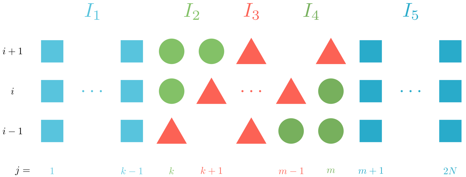
Moreover, using (18 22 R i R_{i} Figure 1
(24) R i = \displaystyle R_{i}= I 1 + I 2 + I 3 + I 4 + I 5 for 3 ≤ i ≤ N . \displaystyle I_{1}+I_{2}+I_{3}+I_{4}+I_{5}\quad\text{for}\quad 3\leq i\leq N.
Here,
I 1 = ∑ j = 1 k − 1 V i j I_{1}=\sum_{j=1}^{k-1}V_{ij} I 3 = ∑ j = k + 1 m − 1 S i j I_{3}=\sum_{j=k+1}^{m-1}S_{ij} I 5 = ∑ j = m + 1 2 N V i j I_{5}=\sum_{j=m+1}^{2N}V_{ij}
I 2 = 2 h i + h i + 1 ( 1 h i + 1 ( T i + 1 , k + T i + 1 , k + 1 ) − ( 1 h i + 1 h i + 1 ) T i , k ) , \displaystyle I_{2}=\frac{2}{h_{i}+h_{i+1}}\left(\frac{1}{h_{i+1}}(T_{i+1,k}+T_{i+1,k+1})-(\frac{1}{h_{i}}+\frac{1}{h_{i+1}})T_{i,k}\right),
I 4 = 2 h i + h i + 1 ( 1 h i ( T i − 1 , m + T i − 1 , m − 1 ) − ( 1 h i + 1 h i + 1 ) T i , m ) \displaystyle I_{4}=\frac{2}{h_{i}+h_{i+1}}\left(\frac{1}{h_{i}}(T_{i-1,m}+T_{i-1,m-1})-(\frac{1}{h_{i}}+\frac{1}{h_{i+1}})T_{i,m}\right)
with
(25) k = ⌈ i / 2 ⌉ , m = { 2 i , 3 ≤ i < N / 2 , 2 N − ⌈ N / 2 ⌉ + 1 , N / 2 ≤ i ≤ N . k=\lceil i/2\rceil,\quad m=\begin{cases}2i,&3\leq i<N/2,\\
2N-\lceil N/2\rceil+1,&N/2\leq i\leq N.\end{cases}
Note that I 1 I_{1} I 5 I_{5} V i j V_{ij} 21 I 3 I_{3} S i j S_{ij} 22
Figure 1: Natural-Skew ordering of R i R_{i}
The complexity in estimating S i j S_{ij} 22 T i − 1 , j − 1 , T i , j T_{i-1,j-1},T_{i,j} T i + 1 , j + 1 T_{i+1,j+1} T i j T_{ij}
Lemma 3.7 .
For any y ∈ ( x j − 1 , x j ) y\in(x_{j-1},x_{j})
T i j \displaystyle T_{ij} = ∫ x j − 1 x j ( u ( y ) − Π h u ( y ) ) K ( x i − y ) 𝑑 y \displaystyle=\int_{x_{j-1}}^{x_{j}}(u(y)-\Pi_{h}u(y))K(x_{i}-y)dy
= ∫ 0 1 − θ ( 1 − θ ) 2 h j 3 u ′′ ( y j θ ) K ( x i − y j θ ) d θ \displaystyle=\int_{0}^{1}-\frac{\theta(1-\theta)}{2}h_{j}^{3}u^{\prime\prime}(y_{j}^{\theta})K(x_{i}-y_{j}^{\theta})d\theta
+ ∫ 0 1 θ ( 1 − θ ) 3 ! h j 4 K ( x i − y j θ ) ( θ 2 u ′′′ ( η j 1 θ ) − ( 1 − θ ) 2 u ′′′ ( η j 2 θ ) ) 𝑑 θ \displaystyle\quad+\int_{0}^{1}\frac{\theta(1-\theta)}{3!}h_{j}^{4}K(x_{i}-y_{j}^{\theta})\left(\theta^{2}u^{\prime\prime\prime}(\eta_{j1}^{\theta})-(1-\theta)^{2}u^{\prime\prime\prime}(\eta_{j2}^{\theta})\right)d\theta
with η j 1 θ ∈ ( x j − 1 , y j θ ) , η j 2 θ ∈ ( y j θ , x j ) \eta_{j1}^{\theta}\in(x_{j-1},y_{j}^{\theta}),\eta_{j2}^{\theta}\in(y_{j}^{\theta},x_{j})
To estimate the local truncation error more concisely, we construct the following grid mapping functions.
Definition 3.9 .
For 1 ≤ i , j ≤ 2 N − 1 1\leq i,j\leq 2N-1
(26) y i , j ( x ) = { ( x 1 / r + Z j − i ) r i < N , j < N , x 1 / r − Z i Z 1 h N + x N i < N , j = N , 2 T − ( Z 2 N − ( j − i ) − x 1 / r ) r i < N , j > N , ( Z 1 h N ( x − x N ) + Z j ) r i = N , j < N , x i = N , j = N , y_{i,j}(x)=\begin{cases}(x^{1/r}+Z_{j-i})^{r}&i<N,j<N,\\
\dfrac{x^{1/r}-Z_{i}}{Z_{1}}h_{N}+x_{N}&i<N,j=N,\\
2T-(Z_{2N-(j-i)}-x^{1/r})^{r}&i<N,j>N,\\
\left(\dfrac{Z_{1}}{h_{N}}(x-x_{N})+Z_{j}\right)^{r}&i=N,j<N,\\
x&i=N,j=N,\\
\end{cases}
and
y i , j ( x ) = { 2 T − ( Z 1 h N ( 2 T − x − x N ) + Z 2 N − j ) r i = N , j > N , ( Z 2 N + j − i − ( 2 T − x ) 1 / r ) r i > N , j < N , Z 2 N − j − ( 2 T − x ) 1 / r Z 1 h N + x N i > N , j = N , 2 T − ( ( 2 T − x ) 1 / r − Z j − i ) r i > N , j > N y_{i,j}(x)=\begin{cases}2T-\left(\dfrac{Z_{1}}{h_{N}}(2T-x-x_{N})+Z_{2N-j}\right)^{r}&i=N,j>N,\\
(Z_{2N+j-i}-(2T-x)^{1/r})^{r}&i>N,j<N,\\
\dfrac{Z_{2N-j}-(2T-x)^{1/r}}{Z_{1}}h_{N}+x_{N}&i>N,j=N,\\
2T-((2T-x)^{1/r}-Z_{j-i})^{r}&i>N,j>N\\
\end{cases}
with Z j := T 1 / r j N Z_{j}:=T^{1/r}\frac{j}{N}
Let us further define
(27) h i , j ( x ) = y i , j ( x ) − y i , j − 1 ( x ) , h_{i,j}(x)=y_{i,j}(x)-y_{i,j-1}(x),
(28) y i , j θ ( x ) = ( 1 − θ ) y i , j − 1 ( x ) + θ y i , j − 1 ( x ) , θ ∈ ( 0 , 1 ) , y_{i,j}^{\theta}(x)=(1-\theta)y_{i,j-1}(x)+\theta y_{i,j-1}(x),\quad\theta\in(0,1),
(29) P i , j θ ( x ) = ( h i , j ( x ) ) 3 K ( x − y i , j θ ( x ) ) u ′′ ( y i , j θ ( x ) ) , {P_{i,j}^{\theta}}(x)=({h_{i,j}}(x))^{3}K(x-{y_{i,j}^{\theta}}(x))u^{\prime\prime}({y_{i,j}^{\theta}}(x)),
(30) Q i , j , l θ ( x ) = ( h i , j ( x ) ) l K ( x − y i , j θ ( x ) ) , l = 3 , 4 . {Q_{i,j,l}^{\theta}}(x)=({h_{i,j}}(x))^{l}K(x-{y_{i,j}^{\theta}}(x)),\quad l=3,4.
Then, we can check that
(31) y i , j ( x i − 1 ) = x j − 1 , y i , j ( x i ) = x j , y i , j ( x i + 1 ) = x j + 1 , h i , j ( x i − 1 ) = h j − 1 , h i , j ( x i ) = h j , h i , j ( x i + 1 ) = h j + 1 , y i , j θ ( x i − 1 ) = y j − 1 θ , y i , j θ ( x i ) = y j θ , y i , j θ ( x i + 1 ) = y j + 1 θ . \begin{gathered}y_{i,j}(x_{i-1})=x_{j-1},\quad y_{i,j}(x_{i})=x_{j},\quad y_{i,j}(x_{i+1})=x_{j+1},\\
h_{i,j}(x_{i-1})=h_{j-1},\quad h_{i,j}(x_{i})=h_{j},\quad h_{i,j}(x_{i+1})=h_{j+1},\\
y_{i,j}^{\theta}(x_{i-1})=y_{j-1}^{\theta},\quad y_{i,j}^{\theta}(x_{i})=y_{j}^{\theta},\quad y_{i,j}^{\theta}(x_{i+1})=y_{j+1}^{\theta}.\end{gathered}
From (29 30 Lemma 3.7 T i j T_{ij}
(32) T i j \displaystyle T_{ij} = ∫ 0 1 − θ ( 1 − θ ) 2 P i , j θ ( x i ) d θ \displaystyle=\int_{0}^{1}-\frac{\theta(1-\theta)}{2}{P_{i,j}^{\theta}}(x_{i})d\theta
+ ∫ 0 1 θ ( 1 − θ ) 3 ! Q i , j , 4 θ ( x i ) [ θ 2 u ′′′ ( η j , 1 θ ) − ( 1 − θ ) 2 u ′′′ ( η j , 2 θ ) ] 𝑑 θ . \displaystyle\quad+\int_{0}^{1}\frac{\theta(1-\theta)}{3!}{Q_{i,j,4}^{\theta}}(x_{i})\left[\theta^{2}u^{\prime\prime\prime}(\eta_{j,1}^{\theta})-(1-\theta)^{2}u^{\prime\prime\prime}(\eta_{j,2}^{\theta})\right]d\theta.
From (9 22 32 1 ≤ i ≤ 2 N − 1 1\leq i\leq 2N-1 2 ≤ j ≤ 2 N − 1 2\leq j\leq 2N-1
(33) S i j \displaystyle S_{ij} = ∫ 0 1 − θ ( 1 − θ ) 2 D h 2 P i , j θ ( x i ) d θ \displaystyle=\int_{0}^{1}-\frac{\theta(1-\theta)}{2}D_{h}^{2}P_{i,j}^{\theta}(x_{i})d\theta
+ ∫ 0 1 θ 3 ( 1 − θ ) 3 ! 2 h i + h i + 1 ( Q i , j , 4 θ ( x i + 1 ) u ′′′ ( η j + 1 , 1 θ ) − Q i , j , 4 θ ( x i ) u ′′′ ( η j , 1 θ ) h i + 1 ) 𝑑 θ \displaystyle\quad+\int_{0}^{1}\frac{\theta^{3}(1-\theta)}{3!}\frac{2}{h_{i}+h_{i+1}}\left(\frac{{Q_{i,j,4}^{\theta}}(x_{i+1})u^{\prime\prime\prime}(\eta_{j+1,1}^{\theta})-{Q_{i,j,4}^{\theta}}(x_{i})u^{\prime\prime\prime}(\eta_{j,1}^{\theta})}{h_{i+1}}\right)d\theta
− ∫ 0 1 θ 3 ( 1 − θ ) 3 ! 2 h i + h i + 1 ( Q i , j , 4 θ ( x i ) u ′′′ ( η j , 1 θ ) − Q i , j , 4 θ ( x i − 1 ) u ′′′ ( η j − 1 , 1 θ ) h i ) 𝑑 θ \displaystyle\quad-\int_{0}^{1}\frac{\theta^{3}(1-\theta)}{3!}\frac{2}{h_{i}+h_{i+1}}\left(\frac{{Q_{i,j,4}^{\theta}}(x_{i})u^{\prime\prime\prime}(\eta_{j,1}^{\theta})-{Q_{i,j,4}^{\theta}}(x_{i-1})u^{\prime\prime\prime}(\eta_{j-1,1}^{\theta})}{h_{i}}\right)d\theta
− ∫ 0 1 θ ( 1 − θ ) 3 3 ! 2 h i + h i + 1 ( Q i , j , 4 θ ( x i + 1 ) u ′′′ ( η j + 1 , 2 θ ) − Q i , j , 4 θ ( x i ) u ′′′ ( η j , 2 θ ) h i + 1 ) 𝑑 θ \displaystyle\quad-\int_{0}^{1}\frac{\theta(1-\theta)^{3}}{3!}\frac{2}{h_{i}+h_{i+1}}\left(\frac{{Q_{i,j,4}^{\theta}}(x_{i+1})u^{\prime\prime\prime}(\eta_{j+1,2}^{\theta})-{Q_{i,j,4}^{\theta}}(x_{i})u^{\prime\prime\prime}(\eta_{j,2}^{\theta})}{h_{i+1}}\right)d\theta
+ ∫ 0 1 θ ( 1 − θ ) 3 3 ! 2 h i + h i + 1 ( Q i , j , 4 θ ( x i ) u ′′′ ( η j , 2 θ ) − Q i , j , 4 θ ( x i − 1 ) u ′′′ ( η j − 1 , 2 θ ) h i ) 𝑑 θ . \displaystyle\quad+\int_{0}^{1}\frac{\theta(1-\theta)^{3}}{3!}\frac{2}{h_{i}+h_{i+1}}\left(\frac{{Q_{i,j,4}^{\theta}}(x_{i})u^{\prime\prime\prime}(\eta_{j,2}^{\theta})-{Q_{i,j,4}^{\theta}}(x_{i-1})u^{\prime\prime\prime}(\eta_{j-1,2}^{\theta})}{h_{i}}\right)d\theta.
Lemma 3.10 .
For any ξ ∈ ( x i − 1 , x i + 1 ) \xi\in(x_{i-1},x_{i+1}) 2 ≤ i , j ≤ 2 N − 2 2\leq i,j\leq 2N-2
ξ ≃ x i , δ ( y i , j ( ξ ) ) ≃ δ ( x j ) , h i , j ( ξ ) ≃ h j , \displaystyle\xi\simeq x_{i},\quad\delta(y_{i,j}(\xi))\simeq\delta(x_{j}),\quad h_{i,j}(\xi)\simeq h_{j},
| y i , j ( ξ ) − ξ | ≃ | x j − x i | , | y i , j − 1 ( ξ ) − ξ | ≃ | x j − 1 − x i | , \displaystyle|y_{i,j}(\xi)-\xi|\simeq|x_{j}-x_{i}|,\quad|y_{i,j-1}(\xi)-\xi|\simeq|x_{j-1}-x_{i}|,
| y i , j θ ( ξ ) − ξ | = ( 1 − θ ) | y i , j − 1 ( ξ ) − ξ | + θ | y i , j ( ξ ) − ξ | ≃ | y j θ − x i | . \displaystyle|y_{i,j}^{\theta}(\xi)-\xi|=(1-\theta)|y_{i,j-1}(\xi)-\xi|+\theta|y_{i,j}(\xi)-\xi|\simeq|y_{j}^{\theta}-x_{i}|.
Lemma 3.11 .
For any ξ ∈ ( x i − 1 , x i + 1 ) \xi\in(x_{i-1},x_{i+1}) 2 ≤ i ≤ N , 2 ≤ j ≤ 2 N − 2 2\leq i\leq N,2\leq j\leq 2N-2
| h i , j ′ ( ξ ) | ≤ C ( r − 1 ) Z 1 x i 1 / r − 1 δ ( x j ) 1 − 2 / r ≤ C ( r − 1 ) h j x i 1 / r − 1 δ ( x j ) − 1 / r , \displaystyle|h_{i,j}^{\prime}(\xi)|\leq C(r-1)Z_{1}x_{i}^{1/r-1}\delta(x_{j})^{1-2/r}\leq C(r-1)h_{j}x_{i}^{1/r-1}\delta(x_{j})^{-1/r},
| ( y i , j ( ξ ) − ξ ) ′ | ≤ C x i − 1 | x j − x i | . \displaystyle\left|(y_{i,j}(\xi)-\xi)^{\prime}\right|\leq Cx_{i}^{-1}|x_{j}-x_{i}|.
Lemma 3.12 .
For any ξ ∈ ( x i − 1 , x i + 1 ) \xi\in(x_{i-1},x_{i+1}) 2 ≤ i ≤ N , 2 ≤ j ≤ 2 N − 2 2\leq i\leq N,2\leq j\leq 2N-2
| y i , j ′′ ( ξ ) | ≤ C ( r − 1 ) { x j − 1 / r x i 1 / r − 2 | x j − x i | , i < N , j < N , x N 1 − 1 / r x i 1 / r − 2 , i < N , j = N , δ ( x j ) 1 − 2 / r x i 1 / r − 2 x N 1 / r , i < N , j > N , δ ( x j ) 1 − 2 / r x N 2 / r − 2 , i = N , j ≠ N , 0 i = N , j = N . |y_{i,j}^{\prime\prime}(\xi)|\leq C(r-1)\begin{cases}x_{j}^{-1/r}x_{i}^{1/r-2}|x_{j}-x_{i}|,&i<N,j<N,\\
x_{N}^{1-1/r}x_{i}^{1/r-2},&i<N,j=N,\\
\delta(x_{j})^{1-2/r}x_{i}^{1/r-2}x_{N}^{1/r},&i<N,j>N,\\
\delta(x_{j})^{1-2/r}x_{N}^{2/r-2},&i=N,j\neq N,\\
0&i=N,j=N.\end{cases}
For 2 ≤ i ≤ N , 3 ≤ j ≤ 2 N − 2 2\leq i\leq N,3\leq j\leq 2N-2
| h i , j ′′ ( ξ ) | ≤ C ( r − 1 ) { Z 1 x i 1 / r − 2 x j − 2 / r ( | x j − x i | + x j ) , i < N , j < N , x i 1 / r − 2 x N 1 − 1 / r , i < N , j = N , N + 1 , Z 1 x i 1 / r − 2 δ ( x j ) 1 − 3 / r x N 1 / r , i < N , j > N + 1 , Z 1 x N 2 / r − 2 δ ( x j ) 1 − 3 / r , i = N , j ≠ N , N + 1 , x N − 1 , i = N , j = N , N + 1 . |h_{i,j}^{\prime\prime}(\xi)|\leq C(r-1)\begin{cases}Z_{1}x_{i}^{1/r-2}x_{j}^{-2/r}(|x_{j}-x_{i}|+x_{j}),&i<N,j<N,\\
x_{i}^{1/r-2}x_{N}^{1-1/r},&i<N,j=N,N+1,\\
Z_{1}x_{i}^{1/r-2}\delta(x_{j})^{1-3/r}x_{N}^{1/r},&i<N,j>N+1,\\
Z_{1}x_{N}^{2/r-2}\delta(x_{j})^{1-3/r},&i=N,j\neq N,N+1,\\
x_{N}^{-1},&i=N,j=N,N+1.\end{cases}
Lemma 3.13 .
Let P i , j θ ( x i ) {P_{i,j}^{\theta}}(x_{i}) 29 D h 2 D_{h}^{2} 9
Case 1
For 3 ≤ i < N , ⌈ i 2 ⌉ + 1 ≤ j ≤ min { 2 i − 1 , N − 1 } 3\leq i<N,\lceil\frac{i}{2}\rceil+1\leq j\leq\min\{2i-1,N-1\} , there exists
| D h 2 P i , j θ ( x i ) | ≤ C h j 3 | y j θ − x i | 1 − α x i α / 2 − 4 . |D_{h}^{2}{P_{i,j}^{\theta}}(x_{i})|\leq Ch_{j}^{3}|y_{j}^{\theta}-x_{i}|^{1-\alpha}x_{i}^{\alpha/2-4}.
Case 2
For N / 2 ≤ i ≤ N N/2\leq i\leq N , j = N , N + 1 j=N,N+1 , there exists
| D h 2 P i , j θ ( ξ ) | ≤ C h j 3 | y j θ − x i | 1 − α + C ( r − 1 ) h j 2 ( | y j θ − x i | 1 − α + h j | y j θ − x i | − α ) . \displaystyle|D_{h}^{2}P_{i,j}^{\theta}(\xi)|\leq Ch_{j}^{3}|y_{j}^{\theta}-x_{i}|^{1-\alpha}+C(r-1)h_{j}^{2}\Big{(}|y_{j}^{\theta}-x_{i}|^{1-\alpha}+h_{j}|y_{j}^{\theta}-x_{i}|^{-\alpha}\Big{)}.
Case 3
For N / 2 ≤ i ≤ N N/2\leq i\leq N , N + 2 ≤ j ≤ 2 N − ⌈ N 2 ⌉ N+2\leq j\leq 2N-\lceil\frac{N}{2}\rceil , there exists
| D h 2 P i , j θ ( ξ ) | ≤ C h j 3 ( | y j θ − x i | 1 − α + ( r − 1 ) | y j θ − x i | − α ) . \displaystyle|D_{h}^{2}P_{i,j}^{\theta}(\xi)|\leq Ch_{j}^{3}\Big{(}|y_{j}^{\theta}-x_{i}|^{1-\alpha}+(r-1)|y_{j}^{\theta}-x_{i}|^{-\alpha}\Big{)}.
Lemma 3.14 .
Let Q i , j , l θ ( x i ) {Q_{i,j,l}^{\theta}}(x_{i}) 30 2 ≤ i ≤ N 2\leq i\leq N 2 ≤ j ≤ 2 N − 2 2\leq j\leq 2N-2 l = 3 , 4 l=3,4
| Q i , j , l θ ( x i + 1 ) u ( l − 1 ) ( η j + 1 θ ) − Q i , j , l θ ( x i ) u ( l − 1 ) ( η j θ ) h i + 1 | \displaystyle\left|\frac{{Q_{i,j,l}^{\theta}}(x_{i+1})u^{(l-1)}(\eta_{j+1}^{\theta})-{Q_{i,j,l}^{\theta}}(x_{i})u^{(l-1)}(\eta_{j}^{\theta})}{h_{i+1}}\right|
≤ C h j l | y j θ − x i | 1 − α x i − 1 δ ( x j ) α / 2 − l + 1 − 1 / r ( x i 1 / r + δ ( x j ) 1 / r ) , \displaystyle\quad\leq Ch_{j}^{l}|y_{j}^{\theta}-x_{i}|^{1-\alpha}x_{i}^{-1}\delta(x_{j})^{\alpha/2-l+1-1/r}(x_{i}^{1/r}+\delta(x_{j})^{1/r}),
and
| Q i , j , l θ ( x i ) u ( l − 1 ) ( η j θ ) − Q i , j , l θ ( x i − 1 ) u ( l − 1 ) ( η j − 1 θ ) h i | \displaystyle\left|\frac{{Q_{i,j,l}^{\theta}}(x_{i})u^{(l-1)}(\eta_{j}^{\theta})-{Q_{i,j,l}^{\theta}}(x_{i-1})u^{(l-1)}(\eta_{j-1}^{\theta})}{h_{i}}\right|
≤ C h j l | y j θ − x i | 1 − α x i − 1 δ ( x j ) α / 2 − l + 1 − 1 / r ( x i 1 / r + δ ( x j ) 1 / r ) \displaystyle\quad\leq Ch_{j}^{l}|y_{j}^{\theta}-x_{i}|^{1-\alpha}x_{i}^{-1}\delta(x_{j})^{\alpha/2-l+1-1/r}(x_{i}^{1/r}+\delta(x_{j})^{1/r})
with η j θ ∈ ( x j − 1 , x j ) \eta_{j}^{\theta}\in(x_{j-1},x_{j})
3.3 Error analysis of R i R_{i}
In this subsection, we estimate the first term of the local truncation error R i R_{i} 18 23 24
(34) K y ( x ) := K ( x − y ) = κ α Γ ( 2 − α ) | x − y | 1 − α , 1 < α < 2 , K_{y}(x):=K(x-y)=\frac{\kappa_{\alpha}}{\Gamma(2-\alpha)}|x-y|^{1-\alpha},\quad 1<\alpha<2,
where the kernel function K ( x ) K(x) 3 κ α \kappa_{\alpha} 13
Lemma 3.15 .
Let I 5 = ∑ j = m + 1 2 N V i j I_{5}=\sum_{j=m+1}^{2N}V_{ij} 24
Case 1
For 1 ≤ i < N / 2 1\leq i<N/2 and m = max { 2 i , 3 } m=\max\{2i,3\} , there exists
∑ j = m + 1 2 N | V i j | ≤ C h 2 x i − α / 2 − 2 / r + { C h 2 , α / 2 − 2 / r + 1 > 0 , C h 2 ln ( N ) , α / 2 − 2 / r + 1 = 0 , C h r α / 2 + r , α / 2 − 2 / r + 1 < 0 . \displaystyle\sum_{j=m+1}^{2N}\left|V_{ij}\right|\leq Ch^{2}x_{i}^{-\alpha/2-2/r}+\begin{cases}Ch^{2},&\alpha/2-2/r+1>0,\\
Ch^{2}\ln(N),&\alpha/2-2/r+1=0,\\
Ch^{r\alpha/2+r},&\alpha/2-2/r+1<0.\end{cases}
Case 2
For N / 2 ≤ i ≤ N N/2\leq i\leq N and m = 2 N − ⌈ N 2 ⌉ + 1 m=2N-\lceil\frac{N}{2}\rceil+1 , there exists
∑ j = m + 1 2 N | V i j | ≤ { C h 2 , α / 2 − 2 / r + 1 > 0 , C h 2 ln ( N ) , α / 2 − 2 / r + 1 = 0 , C h r α / 2 + r , α / 2 − 2 / r + 1 < 0 . \displaystyle\sum_{j=m+1}^{2N}|V_{ij}|\leq\begin{cases}Ch^{2},&\alpha/2-2/r+1>0,\\
Ch^{2}\ln(N),&\alpha/2-2/r+1=0,\\
Ch^{r\alpha/2+r},&\alpha/2-2/r+1<0.\end{cases}
Proof 3.16 .
For 1 ≤ i < N / 2 1\leq i<N/2 m + 1 ≤ j ≤ 2 N m+1\leq j\leq 2N m = max { 2 i , 3 } m=\max\{2i,3\} 20 21 34 Lemmas A.5 B.5
| V i j | \displaystyle|V_{ij}| = | ∫ x j − 1 x j ( u ( y ) − Π h u ( y ) ) D h 2 K y ( x i ) 𝑑 y | ≤ C h 2 ∫ x j − 1 x j δ ( y ) α / 2 − 2 / r | x i − y | − 1 − α 𝑑 y . \displaystyle=\left|\int_{x_{j-1}}^{x_{j}}\left(u(y)-\Pi_{h}u(y)\right)D_{h}^{2}K_{y}(x_{i})dy\right|\leq Ch^{2}\int_{x_{j-1}}^{x_{j}}\delta(y)^{\alpha/2-2/r}|x_{i}-y|^{-1-\alpha}dy.
Since y ≥ x j − 1 ≥ x 2 i y\geq x_{j-1}\geq x_{2i} y − x i ≃ y y-x_{i}\simeq y x i ≃ x 2 i x_{i}\simeq x_{2i}
∑ j = m + 1 N | V i j | \displaystyle\sum_{j=m+1}^{N}|V_{ij}| ≤ C h 2 ∫ x 2 i x N y − α / 2 − 2 / r − 1 𝑑 y ≤ C h 2 x i − α / 2 − 2 / r . \displaystyle\leq Ch^{2}\int_{x_{2i}}^{x_{N}}y^{-\alpha/2-2/r-1}dy\leq Ch^{2}x_{i}^{-\alpha/2-2/r}.
On the other hand, since y − x i ≃ T y-x_{i}\simeq T y ≥ x N = T y\geq x_{N}=T
∑ j = N + 1 2 N − 1 | V i j | \displaystyle\sum_{j=N+1}^{2N-1}|V_{ij}| ≤ C T − 1 − α h 2 ∫ x N x 2 N − 1 ( 2 T − y ) α / 2 − 2 / r 𝑑 y \displaystyle\leq CT^{-1-\alpha}h^{2}\int_{x_{N}}^{x_{2N-1}}(2T-y)^{\alpha/2-2/r}dy
≤ { C α / 2 − 2 / r + 1 T − α / 2 − 2 / r h 2 , α / 2 − 2 / r + 1 > 0 , C r T − 1 − α h 2 ln ( N ) , α / 2 − 2 / r + 1 = 0 , C | α / 2 − 2 / r + 1 | T − α / 2 − 2 / r h r α / 2 + r , α / 2 − 2 / r + 1 < 0 . \displaystyle\leq\begin{cases}\frac{C}{\alpha/2-2/r+1}T^{-\alpha/2-2/r}\;h^{2},&\alpha/2-2/r+1>0,\\
CrT^{-1-\alpha}h^{2}\ln(N),&\alpha/2-2/r+1=0,\\
\frac{C}{|\alpha/2-2/r+1|}T^{-\alpha/2-2/r}\;h^{r\alpha/2+r},&\alpha/2-2/r+1<0.\end{cases}
Finally, by Lemma A.7
| V i , 2 N | ≤ C T − 1 − α h 2 N α / 2 + 1 = C T − α / 2 h r α / 2 + r . |V_{i,2N}|\leq CT^{-1-\alpha}h_{2N}^{\alpha/2+1}=CT^{-\alpha/2}h^{r\alpha/2+r}.
Then, the desired result in Case 1 is obtained.
We can similarly prove for Case 2, the details are omitted here.
Immediately, we can calculate R 1 , R 2 R_{1},R_{2} 23
Lemma 3.17 .
For i = 1 , 2 i=1,2
| R i | ≤ C h 2 x i − α / 2 − 2 / r + { C h 2 , α / 2 − 2 / r + 1 > 0 , C h 2 ln ( N ) , α / 2 − 2 / r + 1 = 0 , C h r α / 2 + r , α / 2 − 2 / r + 1 < 0 . \displaystyle|R_{i}|\leq Ch^{2}x_{i}^{-\alpha/2-2/r}+\begin{cases}Ch^{2},&\alpha/2-2/r+1>0,\\
Ch^{2}\ln(N),&\alpha/2-2/r+1=0,\\
Ch^{r\alpha/2+r},&\alpha/2-2/r+1<0.\end{cases}
For R i R_{i} 3 ≤ i ≤ N 3\leq i\leq N { I 1 , I 2 , I 3 , I 4 } \{I_{1},I_{2},I_{3},I_{4}\} 24
Lemma 3.19 .
Let I 1 = ∑ j = 1 k − 1 V i j I_{1}=\sum_{j=1}^{k-1}V_{ij} 24 3 ≤ i ≤ N , k = ⌈ i 2 ⌉ 3\leq i\leq N,k=\lceil\frac{i}{2}\rceil
∑ j = 1 k − 1 | V i j | ≤ { C h 2 x i − α / 2 − 2 / r , α / 2 − 2 / r + 1 > 0 , C h 2 x i − 1 − α ln ( i ) , α / 2 − 2 / r + 1 = 0 , C h r α / 2 + r x i − 1 − α , α / 2 − 2 / r + 1 < 0 . \sum_{j=1}^{k-1}|V_{ij}|\leq\begin{cases}Ch^{2}x_{i}^{-\alpha/2-2/r},&\alpha/2-2/r+1>0,\\
Ch^{2}x_{i}^{-1-\alpha}\ln(i),&\alpha/2-2/r+1=0,\\
Ch^{r\alpha/2+r}x_{i}^{-1-\alpha},&\alpha/2-2/r+1<0.\end{cases}
Proof 3.20 .
According to (21 Lemmas A.7 B.5
| V i 1 | ≤ C ∫ 0 x 1 x 1 α / 2 | x i − y | − 1 − α 𝑑 y ≃ x 1 α / 2 + 1 x i − 1 − α = T α / 2 + 1 h r α / 2 + r x i − 1 − α . |V_{i1}|\leq C\int_{0}^{x_{1}}x_{1}^{\alpha/2}|x_{i}-y|^{-1-\alpha}dy\simeq x_{1}^{\alpha/2+1}x_{i}^{-1-\alpha}=T^{\alpha/2+1}h^{r\alpha/2+r}x_{i}^{-1-\alpha}.
Using Lemma A.5 Lemma B.5 y ≤ x k − 1 < 2 − r x i y\leq x_{k-1}<2^{-r}x_{i} x i − y ≃ x i x_{i}-y\simeq x_{i}
| V i j | ≤ C h 2 ∫ x j − 1 x j y α / 2 − 2 / r x i − 1 − α 𝑑 y , 2 ≤ j ≤ k − 1 , \displaystyle|V_{ij}|\leq Ch^{2}\int_{x_{j-1}}^{x_{j}}y^{\alpha/2-2/r}x_{i}^{-1-\alpha}dy,\quad 2\leq j\leq k-1,
and
∑ j = 2 k − 1 | V i j | ≤ C h r α / 2 + r x i − 1 − α + C h 2 x i − 1 − α ∫ x 1 x ⌈ i 2 ⌉ − 1 y α / 2 − 2 / r 𝑑 y . \displaystyle\sum_{j=2}^{k-1}|V_{ij}|\leq Ch^{r\alpha/2+r}x_{i}^{-1-\alpha}+Ch^{2}x_{i}^{-1-\alpha}\int_{x_{1}}^{x_{\lceil\frac{i}{2}\rceil-1}}y^{\alpha/2-2/r}dy.
Moreover we can check that
∫ x 1 x ⌈ i 2 ⌉ − 1 y α / 2 − 2 / r 𝑑 y \displaystyle\int_{x_{1}}^{x_{\lceil\frac{i}{2}\rceil-1}}y^{\alpha/2-2/r}dy ≤ { 1 α / 2 − 2 / r + 1 ( 2 − r x i ) α / 2 − 2 / r + 1 , α / 2 − 2 / r + 1 > 0 , ln ( 2 − r x i ) − ln ( x 1 ) , α / 2 − 2 / r + 1 = 0 , 1 | α / 2 − 2 / r + 1 | x 1 α / 2 − 2 / r + 1 , α / 2 − 2 / r + 1 < 0 . \displaystyle\leq\begin{cases}\frac{1}{\alpha/2-2/r+1}(2^{-r}x_{i})^{\alpha/2-2/r+1},&\alpha/2-2/r+1>0,\\
\ln(2^{-r}x_{i})-\ln(x_{1}),&\alpha/2-2/r+1=0,\\
\frac{1}{|\alpha/2-2/r+1|}x_{1}^{\alpha/2-2/r+1},&\alpha/2-2/r+1<0.\end{cases}
The proof is completed.
Subsequently, we turn our attention to I 3 = ∑ j = k + 1 m − 1 S i j I_{3}=\sum_{j=k+1}^{m-1}S_{ij} m = 2 i m=2i 3 ≤ i < N / 2 3\leq i<N/2 m = 2 N − ⌈ N / 2 ⌉ + 1 m=2N-\lceil N/2\rceil+1 N / 2 ≤ i ≤ N N/2\leq i\leq N 25
Lemma 3.21 .
Let I 3 = ∑ j = k + 1 m − 1 S i j I_{3}=\sum_{j=k+1}^{m-1}S_{ij} 24
Case 1
For N / 2 ≤ i ≤ N N/2\leq i\leq N , m = 2 N − ⌈ N / 2 ⌉ + 1 m=2N-\lceil N/2\rceil+1 , there exist
| S i j | ≤ C ( h 3 + ( r − 1 ) h 2 ) ( T − x i + h N ) 1 − α , j = N , N + 1 , |S_{ij}|\leq C(h^{3}+(r-1)h^{2})(T-x_{i}+h_{N})^{1-\alpha},\quad j=N,N+1,
and
∑ j = N + 2 m − 1 | S i j | ≤ C h 2 + C ( r − 1 ) h 2 ( T − x i + h N ) 1 − α . \sum_{j=N+2}^{m-1}\left|S_{ij}\right|\leq Ch^{2}+C(r-1)h^{2}(T-x_{i}+h_{N})^{1-\alpha}.
Case 2
For 3 ≤ i ≤ N − 1 3\leq i\leq N-1 , k = ⌈ i 2 ⌉ k=\lceil\frac{i}{2}\rceil , there exist
∑ j = k + 1 min { m − 1 , N − 1 } | S i j | ≤ C h 2 x i − α / 2 − 2 / r , ∑ j = ⌈ N 2 ⌉ + 1 N − 1 | S N j | ≤ C h 2 + C ( r − 1 ) h 2 h N 1 − α . \sum_{j=k+1}^{\min\{m-1,N-1\}}\left|S_{ij}\right|\leq Ch^{2}x_{i}^{-\alpha/2-2/r},\quad\sum_{j=\lceil\frac{N}{2}\rceil+1}^{N-1}\left|S_{Nj}\right|\leq Ch^{2}+C(r-1)h^{2}h_{N}^{1-\alpha}.
Proof 3.22 .
Case 1: From (33 θ ( 1 − θ ) h j ≤ | y j θ − x i | \theta(1-\theta)h_{j}\leq|y_{j}^{\theta}-x_{i}| Lemmas 3.1 3.13 3.14
| S i j | \displaystyle|S_{ij}| ≤ C ( h j 3 + ( r − 1 ) h j 2 ) ∫ 0 1 | y j θ − x i | 1 − α 𝑑 θ , j = N , N + 1 \displaystyle\leq C(h_{j}^{3}+(r-1)h_{j}^{2})\int_{0}^{1}|y_{j}^{\theta}-x_{i}|^{1-\alpha}d\theta,\quad j=N,N+1
with
∫ 0 1 | y j θ − x i | 1 − α 𝑑 y ≃ ( | x j − x i | + h N ) 1 − α \int_{0}^{1}|y_{j}^{\theta}-x_{i}|^{1-\alpha}dy\simeq(|x_{j}-x_{i}|+h_{N})^{1-\alpha}
On the other hand, for j ≥ N + 2 j\geq N+2 x i ≃ x j ≃ T x_{i}\simeq x_{j}\simeq T
| S i j | \displaystyle|S_{ij}| ≤ C h j 2 ∫ 0 1 ( | y j θ − x i | 1 − α + ( r − 1 ) | y j θ − x i | − α ) h j 𝑑 θ \displaystyle\leq Ch_{j}^{2}\int_{0}^{1}\left(|y_{j}^{\theta}-x_{i}|^{1-\alpha}+(r-1)|y_{j}^{\theta}-x_{i}|^{-\alpha}\right)h_{j}d\theta
≤ C h 2 ∫ x j − 1 x j | y − x i | 1 − α + ( r − 1 ) | y − x i | − α d y . \displaystyle\leq Ch^{2}\int_{x_{j-1}}^{x_{j}}|y-x_{i}|^{1-\alpha}+(r-1)|y-x_{i}|^{-\alpha}dy.
It implies that
∑ j = N + 2 2 N − ⌈ N 2 ⌉ | S i j | \displaystyle\sum_{j=N+2}^{2N-\lceil\frac{N}{2}\rceil}|S_{ij}| = C h 2 ∫ x N + 1 x 2 N − ⌈ N 2 ⌉ | y − x i | 1 − α + ( r − 1 ) | y − x i | − α d y \displaystyle=Ch^{2}\int_{x_{N+1}}^{x_{2N-\lceil\frac{N}{2}\rceil}}|y-x_{i}|^{1-\alpha}+(r-1)|y-x_{i}|^{-\alpha}dy
≤ C h 2 ( T 2 − α + ( r − 1 ) ( T − x i + h N ) 1 − α ) . \displaystyle\leq Ch^{2}\left(T^{2-\alpha}+(r-1)(T-x_{i}+h_{N})^{1-\alpha}\right).
Case 2: for 3 ≤ i ≤ N − 1 3\leq i\leq N-1 k + 1 ≤ j ≤ min { m − 1 , N − 1 } k+1\leq j\leq\min\{m-1,N-1\} Lemmas 3.1 3.13 3.14 x i ≃ x j x_{i}\simeq x_{j} h i ≃ h j h_{i}\simeq h_{j}
| S i j | \displaystyle|S_{ij}| ≤ C h j 2 x i α / 2 − 4 ∫ 0 1 | y j θ − x i | 1 − α h j 𝑑 θ = C h 2 x i α / 2 − 2 − 2 / r ∫ x j − 1 x j | y − x i | 1 − α 𝑑 y , \displaystyle\leq Ch_{j}^{2}x_{i}^{\alpha/2-4}\int_{0}^{1}|y_{j}^{\theta}-x_{i}|^{1-\alpha}h_{j}d\theta=Ch^{2}x_{i}^{\alpha/2-2-2/r}\int_{x_{j-1}}^{x_{j}}|y-x_{i}|^{1-\alpha}dy,
∑ k + 1 min { 2 i − 1 , N − 1 } | S i j | \displaystyle\sum_{k+1}^{\min\{2i-1,N-1\}}|S_{ij}| ≤ C h 2 x i α / 2 − 2 − 2 / r ∫ x k x min { 2 i − 1 , N − 1 } | y − x i | 1 − α 𝑑 y ≤ C h 2 x i − α / 2 − 2 / r . \displaystyle\leq Ch^{2}x_{i}^{\alpha/2-2-2/r}\int_{x_{k}}^{x_{\min\{2i-1,N-1\}}}|y-x_{i}|^{1-\alpha}dy\leq Ch^{2}x_{i}^{-\alpha/2-2/r}.
We can similarly prove the last inequality by Case 1.
The proof is completed.
Finally, we focus our error analysis on the terms I 2 I_{2} I 4 I_{4}
Lemma 3.23 .
Let I 2 , I 4 I_{2},I_{4} 24
Case 1
For 3 ≤ i ≤ N 3\leq i\leq N , k = ⌈ i 2 ⌉ k=\lceil\frac{i}{2}\rceil , there exists
I 2 = 2 h i + h i + 1 ( 1 h i + 1 ( T i + 1 , k + T i + 1 , k + 1 ) − ( 1 h i + 1 h i + 1 ) T i , k ) ≤ C h 2 x i − α / 2 − 2 / r . I_{2}=\frac{2}{h_{i}+h_{i+1}}\left(\frac{1}{h_{i+1}}(T_{i+1,k}+T_{i+1,k+1})-\left(\frac{1}{h_{i}}+\frac{1}{h_{i+1}}\right)T_{i,k}\right)\leq Ch^{2}x_{i}^{-\alpha/2-2/r}.
Case 2
For 3 ≤ i < N / 2 3\leq i<N/2 , m = 2 i m=2i , there exists
I 4 = 2 h i + h i + 1 ( 1 h i ( T i − 1 , 2 i + T i − 1 , 2 i − 1 ) − ( 1 h i + 1 h i + 1 ) T i , 2 i ) ≤ C h 2 x i − α / 2 − 2 / r . I_{4}=\frac{2}{h_{i}+h_{i+1}}\left(\frac{1}{h_{i}}(T_{i-1,2i}+T_{i-1,2i-1})-\left(\frac{1}{h_{i}}+\frac{1}{h_{i+1}}\right)T_{i,2i}\right)\leq Ch^{2}x_{i}^{-\alpha/2-2/r}.
Case 3
For N / 2 ≤ i ≤ N N/2\leq i\leq N , m = N − ⌈ N 2 ⌉ + 1 m=N-\lceil\frac{N}{2}\rceil+1 , there exists
I 4 = 2 h i + h i + 1 ( 1 h i ( T i − 1 , m + T i − 1 , m − 1 ) − ( 1 h i + 1 h i + 1 ) T i , m ) ≤ C h 2 . I_{4}=\frac{2}{h_{i}+h_{i+1}}\left(\frac{1}{h_{i}}(T_{i-1,m}+T_{i-1,m-1})-\left(\frac{1}{h_{i}}+\frac{1}{h_{i+1}}\right)T_{i,m}\right)\leq Ch^{2}.
Proof 3.24 .
Since
(35) 1 h i + 1 ( T i + 1 , k + T i + 1 , k + 1 ) − ( 1 h i + 1 h i + 1 ) T i , k \displaystyle\frac{1}{h_{i+1}}\left(T_{i+1,k}+T_{i+1,k+1}\right)-\left(\frac{1}{h_{i}}+\frac{1}{h_{i+1}}\right)T_{i,k}
= 1 h i + 1 ( T i + 1 , k − T i , k ) + 1 h i + 1 ( T i + 1 , k + 1 − T i , k ) + ( 1 h i + 1 − 1 h i ) T i , k . \displaystyle=\frac{1}{h_{i+1}}\left(T_{i+1,k}-T_{i,k}\right)+\frac{1}{h_{i+1}}\left(T_{i+1,k+1}-T_{i,k}\right)+\left(\frac{1}{h_{i+1}}-\frac{1}{h_{i}}\right)T_{i,k}.
According to x i − x k ≃ x i ≃ x k x_{i}-x_{k}\simeq x_{i}\simeq x_{k} Lemmas A.5 B.5 3.1
1 h i + 1 ( T i + 1 , k − T i , k ) \displaystyle\frac{1}{h_{i+1}}(T_{i+1,k}-T_{i,k}) = ∫ x k − 1 x k ( u ( y ) − Π h u ( y ) ) D h K y ( x i ) 𝑑 y ≤ C h 2 x i − α / 2 − 2 / r h k . \displaystyle=\int_{x_{k-1}}^{x_{k}}(u(y)-\Pi_{h}u(y))D_{h}K_{y}(x_{i})dy\leq Ch^{2}x_{i}^{-\alpha/2-2/r}h_{k}.
From Lemmas A.3 3.7 30
1 h i + 1 ( T i + 1 , k + 1 − T i , k ) \displaystyle\frac{1}{h_{i+1}}\left(T_{i+1,k+1}-T_{i,k}\right) = ∫ 0 1 θ ( θ − 1 ) 2 Q i , k ; 3 θ ( x i + 1 ) u ′′ ( η k + 1 θ ) − Q i , k ; 3 θ ( x i ) u ′′ ( η k θ ) h i + 1 𝑑 θ \displaystyle=\int_{0}^{1}\frac{\theta(\theta-1)}{2}\frac{Q_{i,k;3}^{\theta}(x_{i+1})u^{\prime\prime}(\eta_{k+1}^{\theta})-Q_{i,k;3}^{\theta}(x_{i})u^{\prime\prime}(\eta_{k}^{\theta})}{h_{i+1}}d\theta
with η k θ ∈ ( x k − 1 , x k ) \eta_{k}^{\theta}\in(x_{k-1},x_{k}) η k + 1 θ ∈ ( x k , x k + 1 ) \eta_{k+1}^{\theta}\in(x_{k},x_{k+1}) Lemmas 3.14 3.1
1 h i + 1 | T i + 1 , k + 1 − T i , k | ≤ C h 2 x i − α / 2 − 2 / r h k . \frac{1}{h_{i+1}}|T_{i+1,k+1}-T_{i,k}|\leq Ch^{2}x_{i}^{-\alpha/2-2/r}h_{k}.
For the third term in (35 h i ≃ h k h_{i}\simeq h_{k} Lemmas 3.1 B.1 A.5
h i + 1 − h i h i h i + 1 T i , k ≤ C ( r − 1 ) h 2 x i − α / 2 − 2 / r h k . \displaystyle\frac{h_{i+1}-h_{i}}{h_{i}h_{i+1}}T_{i,k}\leq C(r-1)h^{2}x_{i}^{-\alpha/2-2/r}h_{k}.
Then, the desired result of Case 1 is obtained.
The Case 2 and Case 3 for I 4 I_{4}
Proof 3.26 (Proof of Theorem 3.5
For N / 2 ≤ i ≤ N N/2\leq i\leq N m = 2 N − ⌈ N / 2 ⌉ + 1 m=2N-\lceil N/2\rceil+1 24 I 3 I_{3}
(36) I 3 \displaystyle I_{3} = ∑ j = k + 1 m − 1 S i j = ∑ j = k + 1 N − 1 S i j + ( S i N + S i , N + 1 ) + ∑ j = N + 2 m − 1 S i j . \displaystyle=\sum_{j=k+1}^{m-1}S_{ij}=\sum_{j=k+1}^{N-1}S_{ij}+(S_{iN}+S_{i,N+1})+\sum_{j=N+2}^{m-1}S_{ij}.
According to
Lemma 3.19 Lemma 3.23 Lemma 3.21 Lemma 3.15
4 Convergence analysis
We can now prove our main convergence result for Theorem 2.7
4.1 Some properties of the stiffness matrix
In this subsection, we show some properties of the stiffness matrix A A 12
Lemma 4.1 .
The stiffness matrix A A 12 C A C_{A}
∑ j = 1 2 N − 1 a i j ≥ C A ( x i − α + ( 2 T − x i ) − α ) with C A = κ α ( α − 1 ) Γ ( 2 − α ) 2 − r α . \displaystyle\sum_{j=1}^{2N-1}a_{ij}\geq C_{A}(x_{i}^{-\alpha}+(2T-x_{i})^{-\alpha})\quad\text{with}\quad C_{A}=\frac{\kappa_{\alpha}(\alpha-1)}{\Gamma(2-\alpha)}2^{-r\alpha}.
Proof 4.2 .
From (13
a i i = κ α Γ ( 4 − α ) 4 h i h i + 1 ( h i 2 − α + h i + 1 2 − α − ( h i + h i + 1 ) 2 − α ) > 0 , a_{ii}=\frac{\kappa_{\alpha}}{\Gamma(4-\alpha)}\frac{4}{h_{i}h_{i+1}}\left(h_{i}^{2-\alpha}+h_{i+1}^{2-\alpha}-(h_{i}+h_{i+1})^{2-\alpha}\right)>0,
where we use 1 + t θ > ( 1 + t ) θ 1+t^{\theta}>(1+t)^{\theta} t = h i + 1 h i t=\frac{h_{i+1}}{h_{i}} θ ∈ ( 0 , 1 ) \theta\in(0,1)
Let s = h i − 1 h i s=\frac{h_{i-1}}{h_{i}} t = h i + 1 h i t=\frac{h_{i+1}}{h_{i}} Lemma B.11
a i , i − 1 \displaystyle a_{i,i-1} = − κ α Γ ( 4 − α ) 1 h i − 1 h i h i + 1 ( h i + 1 h i − 1 3 − α − ( h i + h i + 1 ) ( h i − 1 + h i ) 3 − α \displaystyle=\frac{-\kappa_{\alpha}}{\Gamma(4-\alpha)}\frac{1}{h_{i-1}h_{i}h_{i+1}}\Big{(}h_{i+1}h_{i-1}^{3-\alpha}-(h_{i}+h_{i+1})(h_{i-1}+h_{i})^{3-\alpha}
+ h i ( h i − 1 + h i + h i − 1 ) 3 − α + ( h i − 1 + h i ) ( h i + h i + 1 ) h i 2 − α \displaystyle\quad+h_{i}(h_{i-1}+h_{i}+h_{i-1})^{3-\alpha}+(h_{i-1}+h_{i})(h_{i}+h_{i+1})h_{i}^{2-\alpha}
− ( h i − 1 + h i ) ( h i + h i + 1 ) 3 − α + h i − 1 h i + 1 h i 2 − α + h i − 1 h i + 1 3 − α ) < 0 . \displaystyle\quad-(h_{i-1}+h_{i})(h_{i}+h_{i+1})^{3-\alpha}+h_{i-1}h_{i+1}h_{i}^{2-\alpha}+h_{i-1}h_{i+1}^{3-\alpha}\Big{)}<0.
For | i − j | ≥ 2 |i-j|\geq 2 x i + 1 − y x_{i+1}-y x i − y x_{i}-y x i − 1 − y x_{i-1}-y > 0 >0 < 0 <0 y ∈ ( x j − 1 , x j + 1 ) y\in(x_{j-1},x_{j+1}) h i h i + h i + 1 | x i + 1 − y | + h i + 1 h i + h i + 1 | x i − 1 − y | = | x i − y | \frac{h_{i}}{h_{i}+h_{i+1}}|x_{i+1}-y|+\frac{h_{i+1}}{h_{i}+h_{i+1}}|x_{i-1}-y|=|x_{i}-y| x 1 − α x^{1-\alpha} α ∈ ( 1 , 2 ) \alpha\in(1,2)
h i h i + h i + 1 | x i + 1 − y | 1 − α + h i + 1 h i + h i + 1 | x i − 1 − y | 1 − α > | x i − y | 1 − α , \frac{h_{i}}{h_{i}+h_{i+1}}|x_{i+1}-y|^{1-\alpha}+\frac{h_{i+1}}{h_{i}+h_{i+1}}|x_{i-1}-y|^{1-\alpha}>|x_{i}-y|^{1-\alpha},
which implies that D h 2 K y ( x i ) > 0 D_{h}^{2}K_{y}(x_{i})>0 9 34 13
a i j = − D h 2 I 2 − α ϕ j ( x i ) = − ∫ x j − 1 x j + 1 ϕ j ( y ) D h 2 K y ( x i ) 𝑑 y < 0 . a_{ij}=-D_{h}^{2}I^{2-\alpha}\phi_{j}(x_{i})=-\int_{x_{j-1}}^{x_{j+1}}\phi_{j}(y)D_{h}^{2}K_{y}(x_{i})dy<0.
We next prove that the stiffness matrix A A 12 a ~ i j \tilde{a}_{ij} 13
∑ j = 1 2 N − 1 a ~ i j = g 0 ( x i ) + g 2 N ( x i ) \displaystyle\sum_{j=1}^{2N-1}\tilde{a}_{ij}=g_{0}(x_{i})+g_{2N}(x_{i})
with
g 0 ( x ) = − κ α Γ ( 4 − α ) | x − x 0 | 3 − α − | x − x 1 | 3 − α h 1 g_{0}(x)=\frac{-\kappa_{\alpha}}{\Gamma(4-\alpha)}\frac{|x-x_{0}|^{3-\alpha}-|x-x_{1}|^{3-\alpha}}{h_{1}} g 2 N ( x ) = − κ α Γ ( 4 − α ) | x 2 N − x | 3 − α − | x 2 N − 1 − x | 3 − α h 2 N g_{2N}(x)=\frac{-\kappa_{\alpha}}{\Gamma(4-\alpha)}\frac{|x_{2N}-x|^{3-\alpha}-|x_{2N-1}-x|^{3-\alpha}}{h_{2N}} ∑ j = 1 2 N − 1 a i j = D h 2 g 0 ( x i ) + D h 2 g 2 N ( x i ) \sum_{j=1}^{2N-1}a_{ij}=D_{h}^{2}g_{0}(x_{i})+D_{h}^{2}g_{2N}(x_{i}) 13
For i = 1 i=1
D h 2 g 0 ( x 1 ) \displaystyle D_{h}^{2}g_{0}(x_{1}) = 2 κ α 1 + ( 2 r − 1 ) 3 − α + 2 ( 2 r − 1 ) − ( 2 r ) 3 − α Γ ( 4 − α ) 2 r ( 2 r − 1 ) x 1 − α ≥ κ α ( α − 1 ) Γ ( 2 − α ) 2 − r α x 1 − α , \displaystyle=2\kappa_{\alpha}\frac{1+(2^{r}-1)^{3-\alpha}+2(2^{r}-1)-(2^{r})^{3-\alpha}}{\Gamma(4-\alpha)2^{r}(2^{r}-1)}x_{1}^{-\alpha}\!\geq\frac{\kappa_{\alpha}(\alpha-1)}{\Gamma(2-\alpha)}2^{-r\alpha}x_{1}^{-\alpha},
since
h ( t ) = 2 ( 1 + ( t − 1 ) 3 − α + 2 ( t − 1 ) − t 3 − α ) − ( 3 − α ) ( 2 − α ) ( α − 1 ) ( t 2 − α − t 1 − α ) h(t)=2\left(1+(t-1)^{3-\alpha}+2(t-1)-t^{3-\alpha}\right)-(3-\alpha)(2-\alpha)(\alpha-1)(t^{2-\alpha}-t^{1-\alpha}) t = 2 r ≥ 1 t=2^{r}\geq 1 h ( 1 ) = 0 h(1)=0
For i ≥ 2 i\geq 2 Lemma A.1 ξ ∈ ( x i − 1 , x i + 1 ) \xi\in(x_{i-1},x_{i+1}) η ∈ ( x 0 , x 1 ) \eta\in(x_{0},x_{1})
D h 2 g 0 ( x i ) \displaystyle D_{h}^{2}g_{0}(x_{i}) = g 0 ′′ ( ξ ) = − κ α | ξ − x 0 | 1 − α − | ξ − x 1 | 1 − α Γ ( 2 − α ) h 1 = κ α ( α − 1 ) Γ ( 2 − α ) | ξ − η | − α \displaystyle=g_{0}^{\prime\prime}(\xi)=-\kappa_{\alpha}\frac{|\xi-x_{0}|^{1-\alpha}-|\xi-x_{1}|^{1-\alpha}}{\Gamma(2-\alpha)h_{1}}=\frac{\kappa_{\alpha}(\alpha-1)}{\Gamma(2-\alpha)}|\xi-\eta|^{-\alpha}
≥ κ α ( α − 1 ) Γ ( 2 − α ) x i + 1 − α ≥ κ α ( α − 1 ) Γ ( 2 − α ) 2 − r α x i − α . \displaystyle\geq\frac{\kappa_{\alpha}(\alpha-1)}{\Gamma(2-\alpha)}x_{i+1}^{-\alpha}\geq\frac{\kappa_{\alpha}(\alpha-1)}{\Gamma(2-\alpha)}2^{-r\alpha}x_{i}^{-\alpha}.
Then we have
D h 2 g 0 ( x i ) ≥ C A x i − α D_{h}^{2}g_{0}(x_{i})\geq C_{A}x_{i}^{-\alpha} C A = κ α ( α − 1 ) Γ ( 2 − α ) 2 − r α C_{A}=\frac{\kappa_{\alpha}(\alpha-1)}{\Gamma(2-\alpha)}2^{-r\alpha} i ≥ 1 i\geq 1 D h 2 g 2 N ( x i ) ≥ C A ( 2 T − x i ) − α D_{h}^{2}g_{2N}(x_{i})\geq C_{A}(2T-x_{i})^{-\alpha}
Let us first introduce the quasi-preconditioner
(37) G = diag ( δ ( x 1 ) , … , δ ( x 2 N − 1 ) ) , G=\text{diag}(\delta(x_{1}),...,\delta(x_{2N-1})),
where δ ( x ) \delta(x) 14
Lemma 4.3 .
Let B ~ := A G \tilde{B}:=AG A A 12 B ~ = ( b ~ i j ) ∈ ℝ ( 2 N − 1 ) × ( 2 N − 1 ) \tilde{B}=(\tilde{b}_{ij})\in\mathbb{R}^{(2N-1)\times(2N-1)} C B ~ , C B C_{\tilde{B}},C_{B}
∑ j = 1 2 N − 1 b ~ i j ≥ C B ( T − δ ( x i ) + h N ) 1 − α − C B ~ ( x i 1 − α + ( 2 T − x i ) 1 − α ) . \sum_{j=1}^{2N-1}\tilde{b}_{ij}\geq C_{B}(T-\delta(x_{i})+h_{N})^{1-\alpha}-C_{\tilde{B}}(x_{i}^{1-\alpha}+(2T-x_{i})^{1-\alpha}).
with
C B = 2 κ α Γ ( 2 − α ) , C B ~ = κ α Γ ( 2 − α ) 2 r ( α − 1 ) C_{B}=\frac{2\kappa_{\alpha}}{\Gamma(2-\alpha)},\;C_{\tilde{B}}=\frac{\kappa_{\alpha}}{\Gamma(2-\alpha)}2^{r(\alpha-1)}
Proof 4.4 .
From (13 37
b ~ i j = a i j δ ( x j ) = − 2 h i + h i + 1 ( 1 h i + 1 a ~ i + 1 , j − ( 1 h i + 1 h i + 1 ) a ~ i , j + 1 h i a ~ i − 1 , j ) δ ( x j ) . \tilde{b}_{ij}=a_{ij}\delta(x_{j})=-\frac{2}{h_{i}+h_{i+1}}\left(\frac{1}{h_{i+1}}\tilde{a}_{i+1,j}-(\frac{1}{h_{i}}+\frac{1}{h_{i+1}})\tilde{a}_{i,j}+\frac{1}{h_{i}}\tilde{a}_{i-1,j}\right)\delta(x_{j}).
Since
δ ( x ) ≡ Π h δ ( x ) = ∑ j = 1 2 N − 1 ϕ j ( x ) δ ( x j ) \delta(x)\equiv\Pi_{h}\delta(x)=\sum_{j=1}^{2N-1}\phi_{j}(x)\delta(x_{j}) 6 14 a ~ i j \tilde{a}_{ij} 13
∑ j = 1 2 N − 1 a ~ i j δ ( x j ) \displaystyle\sum_{j=1}^{2N-1}\tilde{a}_{ij}\delta(x_{j}) = ∑ j = 1 2 N − 1 I 2 − α ϕ j ( x i ) δ ( x j ) = I 2 − α δ ( x i ) = − p ( x i ) + q ( x i ) \displaystyle=\sum_{j=1}^{2N-1}I^{2-\alpha}\phi_{j}(x_{i})\delta(x_{j})=I^{2-\alpha}\delta(x_{i})=-p(x_{i})+q(x_{i})
with
p ( x ) = 2 κ α Γ ( 4 − α ) | T − x | 3 − α p(x)=\frac{2\kappa_{\alpha}}{\Gamma(4-\alpha)}|T-x|^{3-\alpha} q ( x ) = κ α Γ ( 4 − α ) ( x 3 − α + ( 2 T − x ) 3 − α ) q(x)=\frac{\kappa_{\alpha}}{\Gamma(4-\alpha)}\left(x^{3-\alpha}+(2T-x)^{3-\alpha}\right) ∑ j = 1 2 N − 1 b ~ i j = ∑ j = 1 2 N − 1 a i j δ ( x j ) = D h 2 p ( x i ) − D h 2 q ( x i ) \sum_{j=1}^{2N-1}\tilde{b}_{ij}=\sum_{j=1}^{2N-1}a_{ij}\delta(x_{j})=D_{h}^{2}p(x_{i})-D_{h}^{2}q(x_{i})
For i ≠ N i\neq N Lemma A.1 ξ ∈ ( x i − 1 , x i + 1 ) \xi\in(x_{i-1},x_{i+1})
D h 2 p ( x i ) \displaystyle D_{h}^{2}p(x_{i}) = 2 κ α Γ ( 2 − α ) | T − ξ | 1 − α ≥ 2 κ α Γ ( 2 − α ) ( T − δ ( x i ) + h N ) 1 − α \displaystyle=\frac{2\kappa_{\alpha}}{\Gamma(2-\alpha)}|T-\xi|^{1-\alpha}\geq\frac{2\kappa_{\alpha}}{\Gamma(2-\alpha)}(T-\delta(x_{i})+h_{N})^{1-\alpha}
and for i = N i=N
D h 2 p ( x N ) \displaystyle D_{h}^{2}p(x_{N}) = 4 κ α Γ ( 4 − α ) h N 2 h N 3 − α ≥ C B ( T − δ ( x N ) + h N ) 1 − α . \displaystyle=\frac{4\kappa_{\alpha}}{\Gamma(4-\alpha)h_{N}^{2}}h_{N}^{3-\alpha}\geq C_{B}(T-\delta(x_{N})+h_{N})^{1-\alpha}.
We can similarly prove the following inequality
D h 2 q ( x i ) \displaystyle D_{h}^{2}q(x_{i}) ≤ C B ~ ( x i 1 − α + ( 2 T − x i ) 1 − α ) , i = 1 , ⋯ , 2 N − 1 . \displaystyle\leq C_{\tilde{B}}(x_{i}^{1-\alpha}+(2T-x_{i})^{1-\alpha}),\quad i=1,\cdots,2N-1.
The proof is completed.
Noted that B ~ = A G \tilde{B}=AG Lemma 4.3 ∑ j = 1 2 N − 1 b ~ i j < 0 \sum_{j=1}^{2N-1}\tilde{b}_{ij}<0 x i x_{i} λ I + μ G \lambda I+\mu G
Lemma 4.5 .
Let B := A ( λ I + μ G ) B:=A(\lambda I+\mu G) λ = 1 + 2 r ( α − 1 ) T \lambda=1+2^{r(\alpha-1)}T μ = ( α − 1 ) 2 − r α − 1 \mu=(\alpha-1)2^{-r\alpha-1} B = ( b i j ) ∈ ℝ ( 2 N − 1 ) × ( 2 N − 1 ) B=(b_{ij})\in\mathbb{R}^{(2N-1)\times(2N-1)}
∑ j = 1 2 N − 1 b i j ≥ C A ( ( x i − α + ( 2 T − x i ) − α ) + ( T − δ ( x i ) + h N ) 1 − α ) . \sum_{j=1}^{2N-1}b_{ij}\geq C_{A}\left((x_{i}^{-\alpha}+(2T-x_{i})^{-\alpha})+(T-\delta(x_{i})+h_{N})^{1-\alpha}\right).
Proof 4.6 .
From Lemmas 4.1 4.3
∑ j = 1 2 N − 1 b i j \displaystyle\sum_{j=1}^{2N-1}b_{ij} = ∑ j = 1 2 N − 1 ( λ a i j + μ b ~ i j ) \displaystyle=\sum_{j=1}^{2N-1}\left(\lambda a_{ij}+\mu\tilde{b}_{ij}\right)
≥ λ C A ( x i − α + ( 2 T − x i ) − α ) − μ C B ~ 2 T ( x i − α + ( 2 T − x i ) − α ) \displaystyle\geq\lambda C_{A}\left(x_{i}^{-\alpha}+(2T-x_{i})^{-\alpha}\right)-\mu C_{\tilde{B}}2T\left(x_{i}^{-\alpha}+(2T-x_{i})^{-\alpha}\right)
+ μ C B ( T − δ ( x i ) + h N ) 1 − α , \displaystyle\;\;+\mu C_{B}\left(T-\delta(x_{i})+h_{N}\right)^{1-\alpha},
with λ = 1 + 2 T C B ~ / C B = 1 + 2 r ( α − 1 ) T \lambda=1+2TC_{\tilde{B}}/C_{B}=1+2^{r(\alpha-1)}T μ = C A / C B = ( α − 1 ) 2 − r α − 1 \mu=C_{A}/C_{B}=(\alpha-1)2^{-r\alpha-1}
Let ϵ i = u ( x i ) − u i \epsilon_{i}=u(x_{i})-u_{i} ϵ 0 = ϵ 2 N = 0 \epsilon_{0}=\epsilon_{2N}=0 10 11
(38) A ϵ = τ , A\epsilon=\tau,
where ϵ = [ ϵ 1 , ϵ 2 , … , ϵ 2 N − 1 ] T \epsilon=[\epsilon_{1},\epsilon_{2},...,\epsilon_{2N-1}]^{T} τ = [ τ 1 , τ 2 , … , τ 2 N − 1 ] T \tau=[\tau_{1},\tau_{2},...,\tau_{2N-1}]^{T} τ i \tau_{i} 8
Let λ I + μ G \lambda I+\mu G B = A ( λ I + μ G ) B=A(\lambda I+\mu G) Lemma 4.5 38
B ( λ I + μ G ) − 1 ϵ = τ , i.e. ∑ j = 1 2 N − 1 b i j ϵ j λ + μ δ ( x j ) = τ i . B(\lambda I+\mu G)^{-1}\epsilon=\tau,\quad\text{i.e.}\quad\sum_{j=1}^{2N-1}b_{ij}\frac{\epsilon_{j}}{\lambda+\mu\delta(x_{j})}=\tau_{i}.
Assume that
| ϵ i 0 λ + μ δ ( x i 0 ) | = max 1 ≤ j ≤ 2 N − 1 | ϵ j λ + μ δ ( x j ) | \left|\frac{\epsilon_{i_{0}}}{\lambda+\mu\delta(x_{i_{0}})}\right|=\max\limits_{1\leq j\leq 2N-1}\left|\frac{\epsilon_{j}}{\lambda+\mu\delta(x_{j})}\right| Lemma 4.5 b i i > 0 b_{ii}>0 b i j < 0 , i ≠ j b_{ij}<0,i\neq j
| τ i 0 | \displaystyle|\tau_{i_{0}}| = | ∑ j = 1 2 N − 1 b i 0 , j ϵ j λ + μ δ ( x j ) | ≥ b i 0 , i 0 | ϵ i 0 λ + μ δ ( x i 0 ) | − ∑ j ≠ i 0 | b i 0 , j | | ϵ j λ + μ δ ( x j ) | \displaystyle=\left|\sum_{j=1}^{2N-1}b_{i_{0},j}\frac{\epsilon_{j}}{\lambda+\mu\delta(x_{j})}\right|\geq b_{i_{0},i_{0}}\left|\frac{\epsilon_{i_{0}}}{\lambda+\mu\delta(x_{i_{0}})}\right|-\sum_{j\neq i_{0}}|b_{i_{0},j}|\left|\frac{\epsilon_{j}}{\lambda+\mu\delta(x_{j})}\right|
≥ b i 0 , i 0 | ϵ i 0 λ + μ δ ( x i 0 ) | − ∑ j ≠ i 0 | b i 0 , j | | ϵ i 0 λ + μ δ ( x i 0 ) | = ∑ j = 1 2 N − 1 b i 0 , j | ϵ i 0 λ + μ δ ( x i 0 ) | . \displaystyle\geq b_{i_{0},i_{0}}\left|\frac{\epsilon_{i_{0}}}{\lambda+\mu\delta(x_{i_{0}})}\right|-\sum_{j\neq i_{0}}|b_{i_{0},j}|\left|\frac{\epsilon_{i_{0}}}{\lambda+\mu\delta(x_{i_{0}})}\right|=\sum_{j=1}^{2N-1}b_{i_{0},j}\left|\frac{\epsilon_{i_{0}}}{\lambda+\mu\delta(x_{i_{0}})}\right|.
According to the above inequality, Theorem 2.6 Lemma 4.5
| ϵ i λ + μ δ ( x i ) | ≤ | ϵ i 0 λ + μ δ ( x i 0 ) | ≤ | τ i 0 | ∑ j = 1 2 N − 1 b i 0 , j ≤ C h min { r α 2 , 2 } + C ( r − 1 ) h 2 . \left|\frac{\epsilon_{i}}{\lambda+\mu\delta(x_{i})}\right|\leq\left|\frac{\epsilon_{i_{0}}}{\lambda+\mu\delta(x_{i_{0}})}\right|\leq\frac{|\tau_{i_{0}}|}{\sum_{j=1}^{2N-1}b_{i_{0},j}}\leq Ch^{\min\{\frac{r\alpha}{2},2\}}+C(r-1)h^{2}.
Since λ + μ δ ( x i ) ≤ λ + μ T \lambda+\mu\delta(x_{i})\leq\lambda+\mu T
| ϵ i | ≤ C ( λ + μ T ) h min { r α 2 , 2 } ≤ C ( 1 + ( 2 r ( α − 1 ) + ( α − 1 ) 2 − r α − 1 ) T ) h min { r α 2 , 2 } . |\epsilon_{i}|\leq C(\lambda+\mu T)h^{\min\{\frac{r\alpha}{2},2\}}\leq C\left(1+(2^{r(\alpha-1)}+(\alpha-1)2^{-r\alpha-1})T\right)h^{\min\{\frac{r\alpha}{2},2\}}.
The proof is completed.
From Lemma 2.4 | f ( x ) | ≤ C δ ( x ) − α / 2 |f(x)|\leq C\delta(x)^{-\alpha/2} Lemma 2.4
Theorem 4.8 (Global Error with singualr source term).
Let α ∈ ( 1 , 2 ) \alpha\in(1,2)
| u ( l ) ( x ) | ≤ C δ ( x ) σ − l , l = 0 , 1 , 2 , 3 , 4 , | f ( l ) ( x ) | ≤ C δ ( x ) σ − α − l , l = 0 , 1 , 2 \begin{split}&|u^{(l)}(x)|\leq C\delta(x)^{\sigma-l},l=0,1,2,3,4,\\
&|f^{(l)}(x)|\leq C\delta(x)^{\sigma-\alpha-l},l=0,1,2\end{split}
with σ ∈ ( 0 , α 2 ] \sigma\in(0,\frac{\alpha}{2}] u i u_{i} u ( x i ) u(x_{i}) 7
max 1 ≤ i ≤ 2 N − 1 | u i − u ( x i ) | ≤ C h min { r σ , 2 } \max_{1\leq i\leq 2N-1}|u_{i}-u(x_{i})|\leq Ch^{\min\{r\sigma,2\}}
for some positive constant C = C ( Ω , α , σ , r , f ) C=C(\Omega,\alpha,\sigma,r,f)
Proof 4.9 .
Similar to the performer in Theorems 2.6 2.7
| τ i | \displaystyle|\tau_{i}| = | − D h α Π h u ( x i ) − f ( x i ) | \displaystyle=|-D_{h}^{\alpha}\Pi_{h}u(x_{i})-f(x_{i})|
≤ C h min { r σ , 2 } δ ( x i ) − α + C ( r − 1 ) h 2 ( T − δ ( x i ) + h N ) 1 − α , \displaystyle\leq Ch^{\min\{r\sigma,2\}}\delta(x_{i})^{-\alpha}+C(r-1)h^{2}(T-\delta(x_{i})+h_{N})^{1-\alpha},
and the global error
max 1 ≤ i ≤ 2 N − 1 | u i − u ( x i ) | ≤ C h min { r σ , 2 } \max\limits_{1\leq i\leq 2N-1}|u_{i}-u(x_{i})|\leq Ch^{\min\{r\sigma,2\}}
5 Numerical experiments
We use the difference-quadrature scheme (12 1
5.1 Regular source term
If f ≡ 1 f\equiv 1 [19 , 22 , 27 ] of the problem (1
u ( x ) = 2 − α Γ ( 1 2 ) Γ ( 1 + α 2 ) Γ ( 1 + α 2 ) [ x ( 1 − x ) ] α 2 , x ∈ Ω = ( 0 , 1 ) . u(x)=\frac{2^{-\alpha}\Gamma(\frac{1}{2})}{\Gamma(1+\frac{\alpha}{2})\Gamma(\frac{1+\alpha}{2})}\left[x(1-x)\right]^{\frac{\alpha}{2}},\quad x\in\Omega=(0,1).
In the numerical experiments of this example, we measure the numerical errors by using the maximum nodal error (i.e., the discrete L ∞ L^{\infty}
E N := max 0 ≤ i ≤ 2 N | u ( x i ) − u i | . E^{N}:=\max_{0\leq i\leq 2N}|u(x_{i})-u_{i}|.
The rate of convergence of E N E^{N}
R a t e N = log 2 ( E N / 2 E N ) . Rate^{N}=\log_{2}\left(\frac{E^{N/2}}{E^{N}}\right).
Table 1 12 𝒪 ( h min { r α 2 , 2 } ) \mathcal{O}(h^{\min\{\frac{r\alpha}{2},2\}}) Theorem 2.7
Table 1: Maximum nodal errors showing convergence rate 𝒪 ( h α 2 ) \mathcal{O}(h^{\frac{\alpha}{2}}) r = 1 r=1 𝒪 ( h 2 ) \mathcal{O}(h^{2}) r = 4 / α r=4/\alpha
5.2 Singular source term
We take the singular source term f ( x ) = x σ − α f(x)=x^{\sigma-\alpha} σ ∈ ( 0 , α 2 ] \sigma\in(0,\frac{\alpha}{2}] σ = 0.4 \sigma=0.4 1
R a t e N = log 2 ( E N / 2 E N ) with E N = max 0 ≤ i ≤ N | u i N / 2 − u 2 i N | . Rate^{N}=\log_{2}\left(\frac{E^{N/2}}{E^{N}}\right)\quad\text{with}\quad E^{N}=\max_{0\leq i\leq N}|u^{N/2}_{i}-u^{N}_{2i}|.
Table 2: Maximum nodal errors showing convergence rate 𝒪 ( h σ ) \mathcal{O}(h^{\sigma}) r = 1 r=1 𝒪 ( h 2 ) \mathcal{O}(h^{2}) r = 2 / σ r=2/\sigma
Table 2 12 𝒪 ( h min { r σ , 2 } ) \mathcal{O}(h^{\min\{r\sigma,2\}}) Theorem 4.8
Acknowledgments
This work was supported by the National Natural Science Foundation of China under Grant No. 12471381 and Science Fund for Distinguished Young Scholars of Gansu Province under Grant No. 23JRRA1020.
Appendix A Approximations of difference and interpolation
In this appendix, we provide some approximations for the second-order difference quotients D h 2 D_{h}^{2} u ( x ) − Π h u ( x ) u(x)-\Pi_{h}u(x)
Lemma A.1 .
Let D h 2 D_{h}^{2} 9 g ( x ) ∈ C ( Ω ¯ ) ∩ C 2 ( Ω ) g(x)\in C(\bar{\Omega})\cap C^{2}(\Omega) ξ ∈ ( x i − 1 , x i + 1 ) \xi\in(x_{i-1},x_{i+1}) i = 1 , 2 , … , 2 N − 1 i=1,2,...,2N-1
D h 2 g ( x i ) \displaystyle D_{h}^{2}g(x_{i}) = g ′′ ( ξ ) , ξ ∈ ( x i − 1 , x i + 1 ) . \displaystyle=g^{\prime\prime}(\xi),\quad\xi\in(x_{i-1},x_{i+1}).
Moreover, if g ( x ) ∈ C ( Ω ¯ ) ∩ C 4 ( Ω ) g(x)\in C(\bar{\Omega})\cap C^{4}(\Omega)
D h 2 g ( x i ) = g ′′ ( x i ) + h i + 1 − h i 3 g ′′′ ( x i ) \displaystyle D_{h}^{2}g(x_{i})=g^{\prime\prime}(x_{i})+\frac{h_{i+1}-h_{i}}{3}g^{\prime\prime\prime}(x_{i})
+ 2 h i + h i + 1 ( 1 h i ∫ x i − 1 x i g ′′′′ ( y ) ( y − x i − 1 ) 3 3 ! 𝑑 y + 1 h i + 1 ∫ x i x i + 1 g ′′′′ ( y ) ( x i + 1 − y ) 3 3 ! 𝑑 y ) . \displaystyle+\frac{2}{h_{i}+h_{i+1}}\left(\frac{1}{h_{i}}\int_{x_{i-1}}^{x_{i}}g^{\prime\prime\prime\prime}(y)\frac{(y-x_{i-1})^{3}}{3!}dy+\frac{1}{h_{i+1}}\int_{x_{i}}^{x_{i+1}}g^{\prime\prime\prime\prime}(y)\frac{(x_{i+1}-y)^{3}}{3!}dy\right).
Proof A.2 .
By Taylor series expansion, we obtain
g ( x i − 1 ) = g ( x i ) − ( x i − x i − 1 ) g ′ ( x i ) + ( x i − x i − 1 ) 2 2 g ′′ ( ξ 1 ) , ξ 1 ∈ ( x i − 1 , x i ) , \displaystyle g(x_{i-1})=g(x_{i})-(x_{i}-x_{i-1})g^{\prime}(x_{i})+\frac{(x_{i}-x_{i-1})^{2}}{2}g^{\prime\prime}(\xi_{1}),\quad\xi_{1}\in(x_{i-1},x_{i}),
g ( x i + 1 ) = g ( x i ) + ( x i + 1 − x i ) g ′ ( x i ) + ( x i + 1 − x i ) 2 2 g ′′ ( ξ 2 ) , ξ 2 ∈ ( x i , x i + 1 ) . \displaystyle g(x_{i+1})=g(x_{i})+(x_{i+1}-x_{i})g^{\prime}(x_{i})+\frac{(x_{i+1}-x_{i})^{2}}{2}g^{\prime\prime}(\xi_{2}),\quad\xi_{2}\in(x_{i},x_{i+1}).
From (9
D h 2 g ( x i ) = h i h i + h i + 1 g ′′ ( ξ 1 ) + h i + 1 h i + h i + 1 g ′′ ( ξ 2 ) = g ′′ ( ξ ) , ξ ∈ [ ξ 1 , ξ 2 ] . D_{h}^{2}g(x_{i})=\frac{h_{i}}{h_{i}+h_{i+1}}g^{\prime\prime}(\xi_{1})+\frac{h_{i+1}}{h_{i}+h_{i+1}}g^{\prime\prime}(\xi_{2})=g^{\prime\prime}(\xi),\quad\xi\in[\xi_{1},\xi_{2}].
The second equation can be derived in a similar manner. The proof is completed.
Lemma A.3 .
Let y j θ = ( 1 − θ ) x j − 1 + θ x j , θ ∈ ( 0 , 1 ) y_{j}^{\theta}=(1-\theta)x_{j-1}+\theta x_{j},\theta\in(0,1) 2 ≤ j ≤ 2 N − 1 2\leq j\leq 2N-1
u ( y j θ ) − Π h u ( y j θ ) \displaystyle u(y_{j}^{\theta})-\Pi_{h}u(y_{j}^{\theta}) = − θ ( 1 − θ ) 2 h j 2 u ′′ ( ξ ) , ξ ∈ ( x j − 1 , x j ) , \displaystyle=-\frac{\theta(1-\theta)}{2}h_{j}^{2}u^{\prime\prime}(\xi),\quad\xi\in(x_{j-1},x_{j}),
u ( y j θ ) − Π h u ( y j θ ) = \displaystyle u(y_{j}^{\theta})-\Pi_{h}u(y_{j}^{\theta})= − θ ( 1 − θ ) 2 h j 2 u ′′ ( y j θ ) + θ ( 1 − θ ) 3 ! h j 3 ( θ 2 u ′′′ ( η 1 ) − ( 1 − θ ) 2 u ′′′ ( η 2 ) ) \displaystyle-\frac{\theta(1-\theta)}{2}h_{j}^{2}u^{\prime\prime}(y_{j}^{\theta})+\frac{\theta(1-\theta)}{3!}h_{j}^{3}\left(\theta^{2}u^{\prime\prime\prime}(\eta_{1})-(1-\theta)^{2}u^{\prime\prime\prime}(\eta_{2})\right)
with η 1 ∈ ( x j − 1 , y j θ ) , η 2 ∈ ( y j θ , x j ) \eta_{1}\in(x_{j-1},y_{j}^{\theta}),\eta_{2}\in(y_{j}^{\theta},x_{j})
Proof A.4 .
Using Taylor series expansion, we get
u ( x j − 1 ) = u ( y j θ ) − θ h j u ′ ( y j θ ) + θ 2 h j 2 2 ! u ′′ ( ξ 1 ) , ξ 1 ∈ ( x j − 1 , y j θ ) , \displaystyle u(x_{j-1})=u(y_{j}^{\theta})-\theta h_{j}u^{\prime}(y_{j}^{\theta})+\frac{\theta^{2}h_{j}^{2}}{2!}u^{\prime\prime}(\xi_{1}),\quad\xi_{1}\in(x_{j-1},y_{j}^{\theta}),
u ( x j ) = u ( y j θ ) + ( 1 − θ ) h j u ′ ( y j θ ) + ( 1 − θ ) 2 h j 2 2 ! u ′′ ( ξ 2 ) , ξ 2 ∈ ( y j θ , x j ) , \displaystyle u(x_{j})=u(y_{j}^{\theta})+(1-\theta)h_{j}u^{\prime}(y_{j}^{\theta})+\frac{(1-\theta)^{2}h_{j}^{2}}{2!}u^{\prime\prime}(\xi_{2}),\quad\xi_{2}\in(y_{j}^{\theta},x_{j}),
which implies that
u ( y j θ ) − Π h u ( y j θ ) \displaystyle u(y_{j}^{\theta})-\Pi_{h}u(y_{j}^{\theta}) = u ( y j θ ) − ( 1 − θ ) u ( x j − 1 ) − θ u ( x j ) \displaystyle=u(y_{j}^{\theta})-(1-\theta)u(x_{j-1})-\theta u(x_{j})
= − θ ( 1 − θ ) 2 h j 2 ( θ u ′′ ( ξ 1 ) + ( 1 − θ ) u ′′ ( ξ 2 ) ) \displaystyle=-\frac{\theta(1-\theta)}{2}h_{j}^{2}(\theta u^{\prime\prime}(\xi_{1})+(1-\theta)u^{\prime\prime}(\xi_{2}))
= − θ ( 1 − θ ) 2 h j 2 u ′′ ( ξ ) , ξ ∈ [ ξ 1 , ξ 2 ] . \displaystyle=-\frac{\theta(1-\theta)}{2}h_{j}^{2}u^{\prime\prime}(\xi),\quad\xi\in[\xi_{1},\xi_{2}].
The second equation can be derived in a similar manner.
The proof is completed.
Lemma A.5 .
For any y ∈ ( x j − 1 , x j ) y\in(x_{j-1},x_{j}) 2 ≤ j ≤ 2 N − 1 2\leq j\leq 2N-1
| u ( y ) − Π h u ( y ) | ≤ h j 2 max ξ ∈ [ x j − 1 , x j ] | u ′′ ( ξ ) | ≤ C h 2 δ ( y ) α / 2 − 2 / r . |u(y)-\Pi_{h}u(y)|\leq h_{j}^{2}\max_{\xi\in[x_{j-1},x_{j}]}|u^{\prime\prime}(\xi)|\leq Ch^{2}\delta(y)^{\alpha/2-2/r}.
Lemma A.7 .
For any x ∈ [ x j − 1 , x j ] x\in[x_{j-1},x_{j}] 1 ≤ j ≤ 2 N 1\leq j\leq 2N
| u ( x ) − Π h u ( x ) | \displaystyle|u(x)-\Pi_{h}u(x)| = | x j − x h j ∫ x j − 1 x u ′ ( y ) 𝑑 y − x − x j − 1 h j ∫ x x j u ′ ( y ) 𝑑 y | ≤ ∫ x j − 1 x j | u ′ ( y ) | 𝑑 y . \displaystyle=\!\left|\frac{x_{j}-x}{h_{j}}\int_{x_{j-1}}^{x}u^{\prime}(y)dy-\frac{x-x_{j-1}}{h_{j}}\int_{x}^{x_{j}}u^{\prime}(y)dy\right|\leq\!\int_{x_{j-1}}^{x_{j}}|u^{\prime}(y)|dy.
In particular, we have
| u ( x ) − Π h u ( x ) | ≤ C 2 α h 1 α / 2 |u(x)-\Pi_{h}u(x)|\leq C\frac{2}{\alpha}h_{1}^{\alpha/2} x ∈ ( 0 , x 1 ) ∪ ( x 2 N − 1 , 2 T ) x\in(0,x_{1})\cup(x_{2N-1},2T)
Proof A.8 .
From the definition of Π h u ( x ) \Pi_{h}u(x) 6 u ( x ) = u ( x i ) + ∫ x i x u ′ ( y ) 𝑑 y u(x)=u(x_{i})+\int_{x_{i}}^{x}u^{\prime}(y)dy
Appendix B Bound estimates
Set
h i = x i − x i − 1 h_{i}=x_{i}-x_{i-1} j = 1 , 2 , … , 2 N j=1,2,...,2N h := 1 N h:=\frac{1}{N}
Lemma B.1 .
For i = 1 , 2 , ⋯ , 2 N − 1 i=1,2,\cdots,2N-1 C C
| h i + 1 − h i | ≤ C ( r − 1 ) h 2 δ ( x i ) 1 − 2 / r , r ≥ 1 . |h_{i+1}-h_{i}|\leq C(r-1)h^{2}\delta(x_{i})^{1-2/r},\quad r\geq 1.
Proof B.2 .
According to the definition of h i = x i − x i − 1 h_{i}=x_{i}-x_{i-1} 5
h i + 1 − h i = { T ( ( i + 1 N ) r − 2 ( i N ) r + ( i − 1 N ) r ) , 1 ≤ i ≤ N − 1 , 0 , i = N , − T ( ( 2 N − i − 1 N ) r − 2 ( 2 N − i N ) r + ( 2 N − i + 1 N ) r ) , N + 1 ≤ i ≤ 2 N − 1 . \displaystyle h_{i+1}-h_{i}=\begin{cases}T\left(\left(\frac{i+1}{N}\right)^{r}-2\left(\frac{i}{N}\right)^{r}+\left(\frac{i-1}{N}\right)^{r}\right),&1\leq i\leq N-1,\\
0,&i=N,\\
-T\left(\left(\frac{2N-i-1}{N}\right)^{r}-2\left(\frac{2N-i}{N}\right)^{r}+\left(\frac{2N-i+1}{N}\right)^{r}\right),&N+1\leq i\leq 2N-1.\\
\end{cases}
Since ( i + 1 ) r − 2 i r + ( i − 1 ) r ≃ r ( r − 1 ) i r − 2 (i+1)^{r}-2i^{r}+(i-1)^{r}\simeq r(r-1)i^{r-2} i ≥ 1 i\geq 1
Lemma B.3 .
For 1 ≤ i ≤ 2 N − 1 1\leq i\leq 2N-1 C C
2 h i + h i + 1 | 1 h i ∫ x i − 1 x i f ′′ ( y ) ( y − x i − 1 ) 3 3 ! 𝑑 y + 1 h i + 1 ∫ x i x i + 1 f ′′ ( y ) ( y − x i + 1 ) 3 3 ! 𝑑 y | \displaystyle\frac{2}{h_{i}+h_{i+1}}\left|\frac{1}{h_{i}}\int_{x_{i-1}}^{x_{i}}f^{\prime\prime}(y)\frac{(y-x_{i-1})^{3}}{3!}dy+\frac{1}{h_{i+1}}\int_{x_{i}}^{x_{i+1}}f^{\prime\prime}(y)\frac{(y-x_{i+1})^{3}}{3!}dy\right|
≤ C h 2 δ ( x i ) − α / 2 − 2 / r . \displaystyle\quad\leq Ch^{2}\delta(x_{i})^{-\alpha/2-2/r}.
Proof B.4 .
By Lemma 2.4 1 ≤ i ≤ 2 N − 1 1\leq i\leq 2N-1
| ∫ x i − 1 x i f ′′ ( y ) ( y − x i − 1 ) 3 3 ! 𝑑 y | ≤ C ∫ x i − 1 x i δ ( y ) − α / 2 − 2 ( y − x i − 1 ) 3 𝑑 y . \displaystyle\left|\int_{x_{i-1}}^{x_{i}}f^{\prime\prime}(y)\frac{(y-x_{i-1})^{3}}{3!}dy\right|\leq C\int_{x_{i-1}}^{x_{i}}\delta(y)^{-\alpha/2-2}(y-x_{i-1})^{3}dy.
In particular, for i = 1 i=1
∫ x i − 1 x i δ ( y ) − α / 2 − 2 ( y − x i − 1 ) 3 𝑑 y = ∫ 0 x 1 y 1 − α / 2 𝑑 y = 1 2 − α / 2 x 1 2 − α / 2 ≃ x 1 − α / 2 − 2 h 1 4 . \int_{x_{i-1}}^{x_{i}}\delta(y)^{-\alpha/2-2}(y-x_{i-1})^{3}dy=\int_{0}^{x_{1}}y^{1-\alpha/2}dy=\frac{1}{2-\alpha/2}x_{1}^{2-\alpha/2}\simeq x_{1}^{-\alpha/2-2}h_{1}^{4}.
For 2 ≤ i ≤ 2 N − 1 2\leq i\leq 2N-1 Lemma 3.1
∫ x i − 1 x i δ ( y ) − α / 2 − 2 ( y − x i − 1 ) 3 𝑑 y ≃ ∫ x i − 1 x i δ ( x i ) − α / 2 − 2 ( y − x i − 1 ) 3 𝑑 y ≃ δ ( x i ) − α / 2 − 2 h i 4 \displaystyle\int_{x_{i-1}}^{x_{i}}\delta(y)^{-\alpha/2-2}(y-x_{i-1})^{3}dy\simeq\int_{x_{i-1}}^{x_{i}}\delta(x_{i})^{-\alpha/2-2}(y-x_{i-1})^{3}dy\simeq\delta(x_{i})^{-\alpha/2-2}h_{i}^{4}
The desired result is obtained.
Lemma B.5 .
For all 1 ≤ i ≤ 2 N − 1 1\leq i\leq 2N-1 1 ≤ j ≤ 2 N 1\leq j\leq 2N y ∈ ( x j − 1 , x j ) y\in(x_{j-1},x_{j})
| D h K y ( x i ) | ≃ | x i − y | − α if [ x j − 1 , x j ] ∩ [ x i , x i + 1 ] = ∅ , \displaystyle|D_{h}K_{y}(x_{i})|\simeq|x_{i}-y|^{-\alpha}\quad\text{if}\quad[x_{j-1},x_{j}]\cap[x_{i},x_{i+1}]=\varnothing,
D h 2 K y ( x i ) ≃ | x i − y | − 1 − α if [ x j − 1 , x j ] ∩ [ x i − 1 , x i + 1 ] = ∅ . \displaystyle D_{h}^{2}K_{y}(x_{i})\simeq|x_{i}-y|^{-1-\alpha}\quad\text{if}\quad[x_{j-1},x_{j}]\cap[x_{i-1},x_{i+1}]=\varnothing.
Proof B.6 .
Since x i − 1 − y x_{i-1}-y x i − y x_{i}-y x i + 1 − y x_{i+1}-y Lemma A.1 K y ( x ) = κ α Γ ( 2 − α ) | x − y | 1 − α K_{y}(x)=\frac{\kappa_{\alpha}}{\Gamma(2-\alpha)}|x-y|^{1-\alpha} 34
| D h K y ( x i ) | \displaystyle|D_{h}K_{y}(x_{i})| = κ α ( α − 1 ) Γ ( 2 − α ) | ξ − y | − α , ξ ∈ ( x i , x i + 1 ) , \displaystyle=\frac{\kappa_{\alpha}(\alpha-1)}{\Gamma(2-\alpha)}|\xi-y|^{-\alpha},\quad\xi\in(x_{i},x_{i+1}),
D h 2 K y ( x i ) \displaystyle D_{h}^{2}K_{y}(x_{i}) = κ α α ( α − 1 ) Γ ( 2 − α ) | ξ − y | − 1 − α , ξ ∈ ( x i − 1 , x i + 1 ) . \displaystyle=\frac{\kappa_{\alpha}\alpha(\alpha-1)}{\Gamma(2-\alpha)}|\xi-y|^{-1-\alpha},\quad\xi\in(x_{i-1},x_{i+1}).
Moreover, from | ξ − y | ≃ | x i − y | |\xi-y|\simeq|x_{i}-y|
Lemma B.7 .
There exists a constant C C
∑ j = 1 3 V 1 j ≤ C h 2 x 1 − α / 2 − 2 / r and ∑ j = 1 4 V 2 j ≤ C h 2 x 2 − α / 2 − 2 / r . \displaystyle\sum_{j=1}^{3}V_{1j}\leq Ch^{2}x_{1}^{-\alpha/2-2/r}\quad\text{and}\quad\sum_{j=1}^{4}V_{2j}\leq Ch^{2}x_{2}^{-\alpha/2-2/r}.
Proof B.8 .
According Lemma A.7 Lemma A.5 20 21
T i j ≤ C x 1 2 − α / 2 ≃ h 1 2 h 2 x 1 − α / 2 − 2 / r ≃ h 1 2 h 2 x 2 − α / 2 − 2 / r for 0 ≤ i ≤ 3 , 1 ≤ j ≤ 4 . T_{ij}\leq Cx_{1}^{2-\alpha/2}\simeq h_{1}^{2}\;h^{2}x_{1}^{-\alpha/2-2/r}\simeq h_{1}^{2}\;h^{2}x_{2}^{-\alpha/2-2/r}\quad\text{for}\quad 0\leq i\leq 3,1\leq j\leq 4.
The proof is completed.
Lemma B.9 .
Let a , b > 0 , θ ∈ [ 0 , 1 ] a,b>0,\;\theta\in[0,1] b 1 − θ | a θ − b θ | ≤ | a − b | b^{1-\theta}|a^{\theta}-b^{\theta}|\leq|a-b|
Proof B.10 .
Since | t θ − 1 | ≤ | t − 1 | |t^{\theta}-1|\leq|t-1| t = a b > 0 t=\frac{a}{b}>0
Lemma B.11 .
Let x > 0 , y ≥ 1 x>0,y\geq 1 α ∈ ( 1 , 2 ) \alpha\in(1,2)
f ( x , y ) = \displaystyle f(x,y)= x y ( 1 + x 2 − α + y 2 − α ) + ( 1 + x + y ) 3 − α \displaystyle xy(1+x^{2-\alpha}+y^{2-\alpha})+(1+x+y)^{3-\alpha}
− ( 1 + x ) ( 1 + y ) ( ( 1 + x ) 2 − α + ( 1 + y ) 2 − α − 1 ) > 0 . \displaystyle-(1+x)(1+y)\left((1+x)^{2-\alpha}+(1+y)^{2-\alpha}-1\right)>0.
Proof B.12 .
The first and second derivatives of f ( x , y ) f(x,y) x x
∂ x f ( x , y ) = ( 3 − α ) [ x 2 − α y + ( 1 + x + y ) 2 − α − ( 1 + x ) 2 − α ( 1 + y ) ] + 1 + 2 y + y 3 − α − ( 1 + y ) 3 − α , \displaystyle\begin{aligned} \partial_{x}f(x,y)=&(3-\alpha)\left[x^{2-\alpha}y+(1+x+y)^{2-\alpha}-(1+x)^{2-\alpha}(1+y)\right]\\
&+1+2y+y^{3-\alpha}-(1+y)^{3-\alpha},\end{aligned}
∂ x 2 f ( x , y ) = ( 3 − α ) ( 2 − α ) ( y x 1 − α + ( 1 + x + y ) 1 − α − ( 1 + y ) ( 1 + x ) 1 − α ) . \displaystyle\partial_{x}^{2}f(x,y)=(3-\alpha)(2-\alpha)\left(yx^{1-\alpha}+(1+x+y)^{1-\alpha}-(1+y)(1+x)^{1-\alpha}\right).
Since y 1 + y x + 1 1 + y ( 1 + x + y ) = 1 + x \frac{y}{1+y}x+\frac{1}{1+y}(1+x+y)=1+x x 1 − α x^{1-\alpha} x > 0 x>0 y 1 + y x 1 − α + 1 1 + y ( 1 + x + y ) 1 − α > ( 1 + x ) 1 − α \frac{y}{1+y}x^{1-\alpha}+\frac{1}{1+y}(1+x+y)^{1-\alpha}>(1+x)^{1-\alpha} ∂ x 2 f ( x , y ) > 0 \partial_{x}^{2}f(x,y)>0 ∂ x f ( x , y ) > ∂ x f ( 0 , y ) \partial_{x}f(x,y)>\partial_{x}f(0,y) ∂ x f ( 0 , y ) > 0 \partial_{x}f(0,y)>0 y ≥ 1 y\geq 1 f ( x , y ) > f ( 0 , y ) = 0 f(x,y)>f(0,y)=0
Appendix C Proofs for grid mapping functions
Proof C.1 (Proof of Lemma 3.10
The first two approximations can be derived from (5 31 2 ≤ i , j ≤ 2 N − 2 2\leq i,j\leq 2N-2
We next prove | y i , j ( ξ ) − ξ | ≃ | x j − x i | |y_{i,j}(\xi)-\xi|\simeq|x_{j}-x_{i}| 26 y i , j ( ξ ) − ξ = 0 y_{i,j}(\xi)-\xi=0 i = j i=j i < j i<j y i , j ( ξ ) − ξ ≤ x j + 1 − x i − 1 ≃ x j − x i y_{i,j}(\xi)-\xi\leq x_{j+1}-x_{i-1}\simeq x_{j}-x_{i} | y i , j ( ξ ) − ξ | |y_{i,j}(\xi)-\xi| 26 | y i , j ( ξ ) − ξ | ≥ min { x j − 1 − x i − 1 , x j + 1 − x i + 1 } ≃ | x j − x i | |y_{i,j}(\xi)-\xi|\geq\min\{x_{j-1}-x_{i-1},x_{j+1}-x_{i+1}\}\simeq|x_{j}-x_{i}|
From (26 27 31 h i , j ( ξ ) = y i , j ( ξ ) − y i , j − 1 ( ξ ) = y j − 1 , j ( y i , j − 1 ( ξ ) ) − y i , j − 1 ( ξ ) ≃ x j − x j − 1 = h j . h_{i,j}(\xi)=y_{i,j}(\xi)-y_{i,j-1}(\xi)=y_{j-1,j}(y_{i,j-1}(\xi))-y_{i,j-1}(\xi)\simeq x_{j}-x_{j-1}=h_{j}.
The final estimate can be obtained since y i , j − 1 ( ξ ) − ξ y_{i,j-1}(\xi)-\xi y i , j ( ξ ) − ξ y_{i,j}(\xi)-\xi ( ≥ 0 (\geq 0 ≤ 0 ) \leq 0)
Proof C.2 (Proof of Lemma 3.11
From (27 26
h i , j ′ ( x ) \displaystyle h_{i,j}^{\prime}(x) = { x 1 / r − 1 ( y i , j 1 − 1 / r ( x ) − y i , j − 1 1 − 1 / r ( x ) ) , i < N , j < N , x 1 / r − 1 ( h N r Z 1 − y i , N − 1 1 − 1 / r ( x ) ) , i < N , j = N , x 1 / r − 1 ( ( 2 T − y i , N + 1 ( x ) ) 1 − 1 / r − h N r Z 1 ) , i < N , j = N + 1 , \displaystyle=\begin{cases}x^{1/r-1}\left(y_{i,j}^{1-1/r}(x)-y_{i,j-1}^{1-1/r}(x)\right),&i<N,j<N,\\
x^{1/r-1}\left(\dfrac{h_{N}}{rZ_{1}}-y_{i,N-1}^{1-1/r}(x)\right),&i<N,j=N,\\
x^{1/r-1}\left((2T-y_{i,N+1}(x))^{1-1/r}-\dfrac{h_{N}}{rZ_{1}}\right),&i<N,j=N+1,\\
\end{cases}
and
h i , j ′ ( x ) \displaystyle h_{i,j}^{\prime}(x) = { x 1 / r − 1 ( ( 2 T − y i , j ( x ) ) 1 − 1 / r − ( 2 T − y i , j − 1 ( x ) ) 1 − 1 / r ) , i < N , j > N + 1 , r Z 1 h N ( y N , j 1 − 1 / r ( x ) − y N , j − 1 1 − 1 / r ( x ) ) , i = N , j < N , r Z 1 h N ( h N r Z 1 − y N , N − 1 1 − 1 / r ( x ) ) , i = N , j = N . \displaystyle=\begin{cases}x^{1/r-1}\left((2T-y_{i,j}(x))^{1-1/r}-(2T-y_{i,j-1}(x))^{1-1/r}\right),&i<N,j>N+1,\\
\dfrac{rZ_{1}}{h_{N}}\left(y_{N,j}^{1-1/r}(x)-y_{N,j-1}^{1-1/r}(x)\right),&i=N,j<N,\\
\dfrac{rZ_{1}}{h_{N}}\left(\dfrac{h_{N}}{rZ_{1}}-y_{N,N-1}^{1-1/r}(x)\right),&i=N,j=N.\end{cases}
For 2 ≤ i ≤ N 2\leq i\leq N 2 ≤ j < N 2\leq j<N
(39) y i , j 1 − 1 / r ( ξ ) − y i , j − 1 1 − 1 / r ( ξ ) \displaystyle y_{i,j}^{1-1/r}(\xi)-y_{i,j-1}^{1-1/r}(\xi) ≤ x j + 1 1 − 1 / r − x j − 2 1 − 1 / r \displaystyle\leq x_{j+1}^{1-1/r}-x_{j-2}^{1-1/r}
≤ C T 1 − 1 / r ( r − 1 ) N 1 − r j r − 2 = C ( r − 1 ) Z 1 x j 1 − 2 / r . \displaystyle\leq CT^{1-1/r}(r-1)N^{1-r}j^{r-2}=C(r-1)Z_{1}x_{j}^{1-2/r}.
For 2 ≤ i ≤ N 2\leq i\leq N j = N j=N
(40) h N r Z 1 = T 1 − 1 / r 1 − ( 1 − h ) r r h = η 1 − 1 / r ≃ x N 1 − 1 / r , η ∈ ( x N − 1 , x N ) , \dfrac{h_{N}}{rZ_{1}}=T^{1-1/r}\dfrac{1-(1-h)^{r}}{rh}=\eta^{1-1/r}\simeq x_{N}^{1-1/r},\quad\eta\in(x_{N-1},x_{N}),
we have
| h N r Z 1 − y i , N − 1 1 − 1 / r ( ξ ) | ≤ x N 1 − 1 / r − x N − 2 1 − 1 / r ≃ ( r − 1 ) Z 1 x N 1 − 2 / r |\frac{h_{N}}{rZ_{1}}-y_{i,N-1}^{1-1/r}(\xi)|\leq x_{N}^{1-1/r}-x_{N-2}^{1-1/r}\simeq(r-1)Z_{1}x_{N}^{1-2/r}
For 2 ≤ i ≤ N 2\leq i\leq N N + 1 ≤ j ≤ 2 N − 2 N+1\leq j\leq 2N-2
| h i , j ′ ( ξ ) | ≤ C ( r − 1 ) Z 1 ξ 1 / r − 1 ( 2 T − x j ) 1 − 2 / r . |h_{i,j}^{\prime}(\xi)|\leq C(r-1)Z_{1}\xi^{1/r-1}(2T-x_{j})^{1-2/r}.
Combine with Lemmas 3.1 3.10
On the other hand, from (26 | y i , j ( x ) − x | = sign ( j − i ) ( y i , j ( x ) − x ) |y_{i,j}(x)-x|=\text{sign}(j-i)(y_{i,j}(x)-x) ( y i , j ( x ) − x ) ′ = y i , j ′ ( x ) − 1 (y_{i,j}(x)-x)^{\prime}=y_{i,j}^{\prime}(x)-1
For 2 ≤ i < N 2\leq i<N 2 ≤ j < N 2\leq j<N Lemmas B.9 3.10
ξ 1 / r | y i , j 1 − 1 / r ( ξ ) − ξ 1 − 1 / r | ≤ | y i , j ( ξ ) − ξ | ≃ | x j − x i | . \xi^{1/r}|y_{i,j}^{1-1/r}(\xi)-\xi^{1-1/r}|\leq|y_{i,j}(\xi)-\xi|\simeq|x_{j}-x_{i}|.
For 2 ≤ i < N 2\leq i<N j = N j=N 40 Lemma B.9
(41) η 1 / r | h N r Z 1 − ξ 1 − 1 / r | \displaystyle\eta^{1/r}\left|\frac{h_{N}}{rZ_{1}}-\xi^{1-1/r}\right| ≤ | η − ξ | , η ∈ ( x N − 1 , x N ) \displaystyle\leq|\eta-\xi|,\quad\eta\in(x_{N-1},x_{N})
≤ | x N − x i | + | h N | + | h i + 1 | ≤ 3 | x N − x i | . \displaystyle\leq|x_{N}-x_{i}|+|h_{N}|+|h_{i+1}|\leq 3|x_{N}-x_{i}|.
For 2 ≤ i < N 2\leq i<N N < j ≤ 2 N − 2 N<j\leq 2N-2 Lemma B.9
ξ 1 / r | ( 2 T − y i , j ( ξ ) ) 1 − 1 / r − ξ 1 − 1 / r | ≤ | 2 T − y i , j ( ξ ) − ξ | \displaystyle\xi^{1/r}|(2T-y_{i,j}(\xi))^{1-1/r}-\xi^{1-1/r}|\leq|2T-y_{i,j}(\xi)-\xi|
≤ | 2 T − x j − x i | + | y i , j ( ξ ) − x j | + | ξ − x i | ≤ | 2 T − x j − x i | + 2 h N \displaystyle\quad\leq|2T-x_{j}-x_{i}|+|y_{i,j}(\xi)-x_{j}|+|\xi-x_{i}|\leq|2T-x_{j}-x_{i}|+2h_{N}
≤ | x j − T | + | T − x i | + 2 h N ≤ 2 | x j − x i | . \displaystyle\quad\leq|x_{j}-T|+|T-x_{i}|+2h_{N}\leq 2|x_{j}-x_{i}|.
Similar to proof of (41 y N , N ( x ) − x ≡ 0 y_{N,N}(x)-x\equiv 0
η 1 / r | y N , j 1 − 1 / r ( ξ ) − h N r Z 1 | ≤ C | x j − x N | , i = N , j < N , η 1 / r | ( 2 T − y N , j ( ξ ) ) 1 − 1 / r − h N r Z 1 | ≤ C | x j − x N | , i = N , j > N . \begin{gathered}\eta^{1/r}|y_{N,j}^{1-1/r}(\xi)-\dfrac{h_{N}}{rZ_{1}}|\leq C|x_{j}-x_{N}|,\quad i=N,j<N,\\
\eta^{1/r}|(2T-y_{N,j}(\xi))^{1-1/r}-\frac{h_{N}}{rZ_{1}}|\leq C|x_{j}-x_{N}|,\quad i=N,j>N.\end{gathered}
Thus, using (26 Lemma 3.10
Proof C.3 (Proof of Lemma 3.12
By Definition 3.9 Lemma B.9 40
(42) x j 1 − 1 / r | Z j − i | = x j 1 − 1 / r | x j 1 / r − x i 1 / r | ≤ | x j − x i | , i < N , j < N , Z 2 N − j + i ≤ Z 2 N = 2 T 1 / r , i < N , j > N , h N r Z 1 ≃ x N 1 − 1 / r , i = N , 2 ≤ j ≤ 2 N − 2 . \begin{split}&x_{j}^{1-1/r}|Z_{j-i}|=x_{j}^{1-1/r}|x_{j}^{1/r}-x_{i}^{1/r}|\leq|x_{j}-x_{i}|,\quad i<N,j<N,\\
&Z_{2N-j+i}\leq Z_{2N}=2T^{1/r},\qquad i<N,j>N,\\
&\dfrac{h_{N}}{rZ_{1}}\simeq x_{N}^{1-1/r},\qquad i=N,2\leq j\leq 2N-2.\end{split}
Combine with (26 Lemma 3.10
From (27 h i , j ′′ ( x ) = y i , j ′′ ( x ) − y i , j − 1 ′′ ( x ) h_{i,j}^{\prime\prime}(x)=y_{i,j}^{\prime\prime}(x)-y_{i,j-1}^{\prime\prime}(x) 3 ≤ j ≤ 2 N − 2 3\leq j\leq 2N-2
(43) | y i , j 1 − 2 / r ( ξ ) − y i , j − 1 1 − 2 / r ( ξ ) | ≃ ( r − 2 ) Z 1 x j 1 − 3 / r , | ( 2 T − y i , j ( ξ ) ) 1 − 2 / r − ( 2 T − y i , j − 1 ( ξ ) ) 1 − 2 / r | ≃ ( r − 2 ) Z 1 ( 2 T − x j ) 1 − 3 / r , \begin{gathered}|y_{i,j}^{1-2/r}(\xi)-y_{i,j-1}^{1-2/r}(\xi)|\simeq(r-2)Z_{1}x_{j}^{1-3/r},\\
|(2T-y_{i,j}(\xi))^{1-2/r}-(2T-y_{i,j-1}(\xi))^{1-2/r}|\simeq(r-2)Z_{1}(2T-x_{j})^{1-3/r},\\
\end{gathered}
which can be similarly proven as (39
For 2 ≤ i < N 2\leq i<N 3 ≤ j < N 3\leq j<N
y i , j 1 − 2 / r ( ξ ) Z j − i − y i , j − 1 1 − 2 / r ( ξ ) Z j − i − 1 = ( y i , j 1 − 2 / r ( ξ ) − y i , j − 1 1 − 2 / r ( ξ ) ) Z j − i + y i , j − 1 1 − 2 / r ( ξ ) Z 1 . \displaystyle y_{i,j}^{1-2/r}(\xi)Z_{j-i}-y_{i,j-1}^{1-2/r}(\xi)Z_{j-i-1}=\left(y_{i,j}^{1-2/r}(\xi)-y_{i,j-1}^{1-2/r}(\xi)\right)Z_{j-i}+y_{i,j-1}^{1-2/r}(\xi)Z_{1}.
Combine with (42 43
| y i , j 1 − 2 / r ( ξ ) Z j − i − y i , j − 1 1 − 2 / r ( ξ ) Z j − i − 1 | ≤ C Z 1 ( | r − 2 | x j − 2 / r | x j − x i | + x j 1 − 2 / r ) . |y_{i,j}^{1-2/r}(\xi)Z_{j-i}-y_{i,j-1}^{1-2/r}(\xi)Z_{j-i-1}|\leq CZ_{1}\left(|r-2|x_{j}^{-2/r}|x_{j}-x_{i}|+x_{j}^{1-2/r}\right).
For 2 ≤ i < N 2\leq i<N j = N , N + 1 j=N,N+1
| h i , j ′′ ( x ) | ≤ | y i , j ′′ ( x ) | + | y i , j − 1 ′′ ( x ) | ≤ C ( r − 1 ) x i 1 / r − 2 x N 1 − 1 / r . |h_{i,j}^{\prime\prime}(x)|\leq|y_{i,j}^{\prime\prime}(x)|+|y_{i,j-1}^{\prime\prime}(x)|\leq C(r-1)x_{i}^{1/r-2}x_{N}^{1-1/r}.
For 2 ≤ i < N 2\leq i<N j > N + 1 j>N+1 Lemma 3.1 43
| δ ( y i , j ( ξ ) ) 1 − 2 / r Z 2 N − ( j − i ) − δ ( y i , j − 1 ( ξ ) ) 1 − 2 / r Z 2 N − ( j − i − 1 ) | \displaystyle\left|\delta(y_{i,j}(\xi))^{1-2/r}Z_{2N-(j-i)}-\delta(y_{i,j-1}(\xi))^{1-2/r}Z_{2N-(j-i-1)}\right|
≤ C Z 1 ( | r − 2 | δ ( x j ) 1 − 3 / r x N 1 / r + δ ( x j ) 1 − 2 / r ) ≤ C Z 1 δ ( x j ) 1 − 3 / r x N 1 / r . \displaystyle\leq CZ_{1}\left(|r-2|\delta(x_{j})^{1-3/r}x_{N}^{1/r}+\delta(x_{j})^{1-2/r}\right)\leq CZ_{1}\delta(x_{j})^{1-3/r}x_{N}^{1/r}.
For i = N , j = N , N + 1 i=N,j=N,N+1 | h N , j ′′ ( ξ ) | ≤ C x N − 1 |h_{N,j}^{\prime\prime}(\xi)|\leq Cx_{N}^{-1} i = N i=N j ≠ N , N + 1 j\neq N,N+1 43 26 Lemma 3.10
Proof C.4 (Proof of Lemma 3.13
According to | y i , j θ ( ξ ) − ξ | = sign ( j − i − 1 + θ ) ( y i , j θ ( ξ ) − ξ ) |y_{i,j}^{\theta}(\xi)-\xi|=\text{sign}(j-i-1+\theta)(y_{i,j}^{\theta}(\xi)-\xi) θ ∈ ( 0 , 1 ) \theta\in(0,1) Lemma A.1 3 29 D h 2 P i , j θ ( x i ) = P i , j θ ′′ ( ξ ) , ξ ∈ ( x i − 1 , x i + 1 ) D_{h}^{2}{P_{i,j}^{\theta}}(x_{i})={P_{i,j}^{\theta}}^{\prime\prime}(\xi),\quad\xi\in(x_{i-1},x_{i+1}) Lemmas 3.10 26 3.11 3.12 2.4 3.1 i , j i,j
h i , j ( ξ ) ≤ C h j , | h i , j ′ ( ξ ) | ≤ C ( r − 1 ) h j x i − 1 , \displaystyle h_{i,j}(\xi)\leq Ch_{j},\quad|h_{i,j}^{\prime}(\xi)|\leq C(r-1)h_{j}x_{i}^{-1},
| y i , j θ ( ξ ) − ξ | ≤ C | y j θ − x i | , | ( y i . j θ ( ξ ) − x i ) ′ | ≤ C | y j θ − x i | x i − 1 , \displaystyle|y_{i,j}^{\theta}(\xi)-\xi|\leq C|y_{j}^{\theta}-x_{i}|,\quad\left|(y_{i.j}^{\theta}(\xi)-x_{i})^{\prime}\right|\leq C|y_{j}^{\theta}-x_{i}|x_{i}^{-1},
| u ′′ ( y i , j θ ( ξ ) ) | ≤ C x i α / 2 − 2 , | ( u ′′ ( y i , j θ ( ξ ) ) ) ′ | ≤ C x i α / 2 − 3 , | ( u ′′ ( y i , j θ ( ξ ) ) ) ′′ | ≤ C x i α / 2 − 4 . \displaystyle\left|u^{\prime\prime}(y_{i,j}^{\theta}(\xi))\right|\leq Cx_{i}^{\alpha/2-2},\;\left|\left(u^{\prime\prime}(y_{i,j}^{\theta}(\xi))\right)^{\prime}\right|\leq Cx_{i}^{\alpha/2-3},\;\left|\left(u^{\prime\prime}(y_{i,j}^{\theta}(\xi))\right)^{\prime\prime}\right|\leq Cx_{i}^{\alpha/2-4}.
By Lemma 3.12
| h i , j ′′ ( ξ ) | \displaystyle|h_{i,j}^{\prime\prime}(\xi)| ≤ C ( r − 1 ) h j x i − 2 , \displaystyle\leq C(r-1)h_{j}x_{i}^{-2},\quad | ( y i , j θ ( ξ ) − x i ) ′′ | ≤ C ( r − 1 ) | y j θ − x i | x i − 2 , \displaystyle\left|(y_{i,j}^{\theta}(\xi)-x_{i})^{\prime\prime}\right|\leq C(r-1)|y_{j}^{\theta}-x_{i}|x_{i}^{-2},\quad for Case 1 , \displaystyle\text{for Case 1},
| h i , j ′′ ( ξ ) | \displaystyle|h_{i,j}^{\prime\prime}(\xi)| ≤ C ( r − 1 ) , \displaystyle\leq C(r-1),\quad | ( y i , j θ ( ξ ) − x i ) ′′ | ≤ C ( r − 1 ) , \displaystyle\left|(y_{i,j}^{\theta}(\xi)-x_{i})^{\prime\prime}\right|\leq C(r-1),\quad for Case 2 , \displaystyle\text{for Case 2},
| h i , j ′′ ( ξ ) | \displaystyle|h_{i,j}^{\prime\prime}(\xi)| ≤ C ( r − 1 ) h j , \displaystyle\leq C(r-1)h_{j},\quad | ( y i , j θ ( ξ ) − x i ) ′′ | ≤ C ( r − 1 ) , \displaystyle\left|(y_{i,j}^{\theta}(\xi)-x_{i})^{\prime\prime}\right|\leq C(r-1),\quad for Case 3 . \displaystyle\text{for Case 3}.
Using Leibniz formula and chain rules, the desired results are obtained.
Proof C.5 (Proof of Lemma 3.14
Since
Q i , j , l θ ( x i + 1 ) u ′′′ ( η j + 1 θ ) − Q i , j , l θ ( x i ) u ′′′ ( η j θ ) h i + 1 \displaystyle\frac{{Q_{i,j,l}^{\theta}}(x_{i+1})u^{\prime\prime\prime}(\eta_{j+1}^{\theta})-{Q_{i,j,l}^{\theta}}(x_{i})u^{\prime\prime\prime}(\eta_{j}^{\theta})}{h_{i+1}}
= Q i , j , l θ ( x i + 1 ) − Q i , j , l θ ( x i ) h i + 1 u ′′′ ( η j + 1 θ ) + Q i , j , l θ ( x i ) u ′′′ ( η j + 1 θ ) − u ′′′ ( η j θ ) h i + 1 . \displaystyle\quad=\frac{Q_{i,j,l}^{\theta}(x_{i+1})-Q_{i,j,l}^{\theta}(x_{i})}{h_{i+1}}u^{\prime\prime\prime}(\eta_{j+1}^{\theta})+Q_{i,j,l}^{\theta}(x_{i})\frac{u^{\prime\prime\prime}(\eta_{j+1}^{\theta})-u^{\prime\prime\prime}(\eta_{j}^{\theta})}{h_{i+1}}.
There exists ξ ∈ ( x i , x i + 1 ) \xi\in(x_{i},x_{i+1}) Q i , j , l θ ( x i + 1 ) − Q i , j , l θ ( x i ) h i + 1 = Q i , j , l θ ′ ( ξ ) \frac{Q_{i,j,l}^{\theta}(x_{i+1})-Q_{i,j,l}^{\theta}(x_{i})}{h_{i+1}}={Q_{i,j,l}^{\theta}}^{\prime}(\xi) 30 Lemmas 3.10 3.11 3.1
| Q i , j , l θ ′ ( ξ ) | ≤ C h j l | y j θ − x i | 1 − α ( x i − 1 + x i 1 / r − 1 δ ( x j ) − 1 / r ) , Q i , j , l θ ( x i ) = C h j l | y j θ − x i | 1 − α . \displaystyle|{Q_{i,j,l}^{\theta}}^{\prime}(\xi)|\leq Ch_{j}^{l}|y_{j}^{\theta}-x_{i}|^{1-\alpha}(x_{i}^{-1}+x_{i}^{1/r-1}\delta(x_{j})^{-1/r}),\;\;Q_{i,j,l}^{\theta}(x_{i})=Ch_{j}^{l}|y_{j}^{\theta}-x_{i}|^{1-\alpha}.
According to Lemmas 3.1 2.4 | u ( l − 1 ) ( η j + 1 θ ) | ≤ C δ ( x j ) α / 2 − l + 1 |u^{(l-1)}(\eta_{j+1}^{\theta})|\leq C\delta(x_{j})^{\alpha/2-l+1}
| u ( l − 1 ) ( η j + 1 θ ) − u ( l − 1 ) ( η j θ ) | h i + 1 \displaystyle\frac{|u^{(l-1)}(\eta_{j+1}^{\theta})-u^{(l-1)}(\eta_{j}^{\theta})|}{h_{i+1}} = | u ( l ) ( η ) | η j + 1 θ − η j θ h i + 1 , η ∈ ( x j − 1 , x j + 1 ) \displaystyle=|u^{(l)}(\eta)|\frac{\eta_{j+1}^{\theta}-\eta_{j}^{\theta}}{h_{i+1}},\quad\eta\in(x_{j-1},x_{j+1})
≤ C δ ( η ) α / 2 − l x j + 1 − x j − 1 h i + 1 ≃ x i 1 / r − 1 δ ( x j ) α / 2 − l + 1 − 1 / r . \displaystyle\leq C\delta(\eta)^{\alpha/2-l}\frac{x_{j+1}-x_{j-1}}{h_{i+1}}\simeq x_{i}^{1/r-1}\delta(x_{j})^{\alpha/2-l+1-1/r}.
Thus, the first inequality is obtained.
The second one can be similarly proven.
References
[1]
G. Acosta, J. P. Borthagaray, O. Bruno, and M. Maas , Regularity theory and high order numerical methods for the (1D)-fractional Laplacian , Math. Comp., 87 (2018), pp. 1821–1857.
[2]
F. Andreu-Vaillo, J. M. Mazón, J. D. Rossi, and J. J. Toledo-Melero , Nonlocal diffusion problems , vol. 165 of Mathematical Surveys and Monographs, American Mathematical Society, Providence, RI; Real Sociedad Matemática Española, Madrid, 2010.
[3]
J. Bertoin , Lévy processes , vol. 121 of Cambridge Tracts in Mathematics, Cambridge University Press, Cambridge, 1996.
[4]
A. Bonito, W. Lei, and J. E. Pasciak , Numerical approximation of the integral fractional Laplacian , Numer. Math., 142 (2019), pp. 235–278.
[5]
W. Bu, Y. Tang, and J. Yang , Galerkin finite element method for two-dimensional Riesz space fractional diffusion equations , J. Comput. Phys., 276 (2014), pp. 26–38.
[6]
C. Çelik and M. Duman , Crank-Nicolson method for the fractional diffusion equation with the Riesz fractional derivative , J. Comput. Phys., 231 (2012), pp. 1743–1750.
[7]
M. Chen and W. Deng , Fourth order accurate scheme for the space fractional diffusion equations , SIAM J. Numer. Anal., 52 (2014), pp. 1418–1438.
[8]
M. Chen and W. Deng , A second-order numerical method for two-dimensional two-sided space fractional convection diffusion equation , Appl. Math. Model., 38 (2014), pp. 3244–3259.
[9]
M. Chen and W. Deng , High order algorithms for the fractional substantial diffusion equation with truncated Lévy flights , SIAM J. Sci. Comput., 37 (2015), pp. A890–A917.
[10]
M. Chen, W. Deng, C. Min, J. Shi, and M. Stynes , Error analysis of a collocation method on graded meshes for a fractional Laplacian problem , Adv. Comput. Math., 50 (2024), pp. Paper No. 49, 27.
[11]
M. Chen, W. Deng, and Y. Wu , Superlinearly convergent algorithms for the two-dimensional space-time Caputo-Riesz fractional diffusion equation , Appl. Numer. Math., 70 (2013), pp. 22–41.
[12]
M. Chen, Y. Wang, X. Cheng, and W. Deng , Second-order LOD multigrid method for multidimensional Riesz fractional diffusion equation , BIT, 54 (2014), pp. 623–647.
[13]
A. de Pablo, F. Quirós, A. Rodríguez, and J. L. Vázquez , A fractional porous medium equation , Adv. Math., 226 (2011), pp. 1378–1409.
[14]
B. Deng, Z. Zhang, and X. Zhao , Superconvergence points for the spectral interpolation of Riesz fractional derivatives , J. Sci. Comput., 81 (2019), pp. 1577–1601.
[15]
W. Deng , Finite element method for the space and time fractional Fokker-Planck equation , SIAM J. Numer. Anal., 47 (2008/09), pp. 204–226.
[16]
H. Ding and C. Li , High-order algorithms for Riesz derivative and their applications (IV) , Fract. Calc. Appl. Anal., 22 (2019), pp. 1537–1560.
[17]
V. J. Ervin, N. Heuer, and J. P. Roop , Regularity of the solution to 1-D fractional order diffusion equations , Math. Comp., 87 (2018), pp. 2273–2294.
[18]
P. Gatto and J. S. Hesthaven , Numerical approximation of the fractional Laplacian via h p hp , J. Sci. Comput., 65 (2015), pp. 249–270.
[19]
R. K. Getoor , First passage times for symmetric stable processes in space , Trans. Amer. Math. Soc., 101 (1961), pp. 75–90.
[20]
D. Gilbarg and N. S. Trudinger , Elliptic partial differential equations of second order , Grundlehren der Mathematischen Wissenschaften, Vol. 224, Springer-Verlag, Berlin-New York, 1977.
[21]
R. Han and S. Wu , A monotone discretization for integral fractional Laplacian on bounded Lipschitz domains: pointwise error estimates under Hölder regularity , SIAM J. Numer. Anal., 60 (2022), pp. 3052–3077.
[22]
Y. Huang and A. Oberman , Numerical methods for the fractional Laplacian: a finite difference–quadrature approach , SIAM J. Numer. Anal., 52 (2014), pp. 3056–3084.
[23]
M. Kwaśnicki , Ten equivalent definitions of the fractional Laplace operator , Fract. Calc. Appl. Anal., 20 (2017), pp. 7–51.
[24]
R. J. LeVeque , Finite difference methods for ordinary and partial differential equations , Society for Industrial and Applied Mathematics (SIAM), Philadelphia, PA, 2007.
Steady-state and time-dependent problems.
[25]
A. Lischke, G. Pang, M. Gulian, and et al. , What is the fractional Laplacian? A comparative review with new results , J. Comput. Phys., 404 (2020), pp. 109009, 62.
[26]
R. Metzler and J. Klafter , The random walk’s guide to anomalous diffusion: a fractional dynamics approach , Phys. Rep., 339 (2000), p. 77.
[27]
X. Ros-Oton and J. Serra , The Dirichlet problem for the fractional Laplacian: regularity up to the boundary , J. Math. Pures Appl. (9), 101 (2014), pp. 275–302.
[28]
X. Ros-Oton and J. Serra , The dirichlet problem for the fractional laplacian: Regularity up to the boundary , Journal de Mathématiques Pures et Appliquées, 101 (2014), pp. 275–302.
[29]
Z.-H. She, C.-X. Lao, H. Yang, and F.-R. Lin , Banded preconditioners for Riesz space fractional diffusion equations , J. Sci. Comput., 86 (2021), pp. Paper No. 31, 22.
[30]
S. Shen, F. Liu, V. Anh, and I. Turner , The fundamental solution and numerical solution of the Riesz fractional advection-dispersion equation , IMA J. Appl. Math., 73 (2008), pp. 850–872.
[31]
J. Shi and M. Chen , High-order BDF convolution quadrature for subdiffusion models with a singular source term , SIAM J. Numer. Anal., 61 (2023), pp. 2559–2579.
[32]
J. Shi, M. Chen, and J. Cao , High-order BDF convolution quadrature for fractional evolution equations with hyper-singular source term , J. Sci. Comput., 101 (2024), pp. Paper No. 9, 22.
[33]
E. Sousa and C. Li , A weighted finite difference method for the fractional diffusion equation based on the Riemann-Liouville derivative , Appl. Numer. Math., 90 (2015), pp. 22–37.
[34]
V. Tarasov , Fractional Dynamics: Application of Fractional Calculus to Dynamics of Particles, Fields and Media , Springer Berlin, Heidelberg, 10 2011.
[35]
V. E. Tarasov , Fractional dynamics , Nonlinear Physical Science, Springer, Heidelberg; Higher Education Press, Beijing, 2010.
Applications of fractional calculus to dynamics of particles, fields and media.
[36]
W. Tian, H. Zhou, and W. Deng , A class of second order difference approximations for solving space fractional diffusion equations , Math. Comp., 84 (2015), pp. 1703–1727.
[37]
E. Valdinoci , From the long jump random walk to the fractional Laplacian , Bol. Soc. Esp. Mat. Apl. SeMA, (2009), pp. 33–44.
[38]
N. Wang, Z. Mao, C. Huang, and G. E. Karniadakis , A spectral penalty method for two-sided fractional differential equations with general boundary conditions , SIAM J. Sci. Comput., 41 (2019), pp. A1840–A1866.
[39]
Q. Yang, F. Liu, and I. Turner , Numerical methods for fractional partial differential equations with Riesz space fractional derivatives , Appl. Math. Model., 34 (2010), pp. 200–218.
[40]
F. Zeng, F. Liu, C. Li, K. Burrage, I. Turner, and V. Anh , A Crank-Nicolson ADI spectral method for a two-dimensional Riesz space fractional nonlinear reaction-diffusion equation , SIAM J. Numer. Anal., 52 (2014), pp. 2599–2622.
[41]
H. Zhou and W. Tian , Two time-stepping schemes for sub-diffusion equations with singular source terms , J. Sci. Comput., 92 (2022), pp. Paper No. 70, 28.