Trace Ratio vs Ratio Trace methods for multi dimensionality reduction

Abstract

In this paper, we introduce a higher order approach for dimension reduction based on the Trace Ratio problem. We show the existence and uniqueness of the solution, and we provide a relationship between the Trace Ratio problem and the Ratio Trace problem. We also propose a new algorithm to solve the Trace Ratio problem. We apply the approach to generalize the Linear Discriminant Analysis (LDA) to higher order tensors. We provide some numerical experiments to illustrate the efficiency of the proposed method. The method is based on the Einstein product, and it is a generalization of the state-of-the-art trace based DR methods to higher order tensors. The superiority of the Tensor-based methods have been shown experimentally, which motivates us to extend the state-of-the-art Ratio Trace based DR methods to higher order tensors via the Einstein product.

1 Introduction

Numerous applications in machine learning and pattern recognition [5] necessitate the handling of data in high-dimensional spaces. However, working with such high-dimensional data can pose significant challenges, including increased computational time, storage requirements, and susceptibility to noise. To address these issues and enhance the efficiency of model training, we often resort to dimensionality reduction (DR) techniques.
Reducing the dimensionality of the data not only helps to alleviate the computational burden but also improves the clarity and interpretability of the models we develop. Interestingly, research has shown that many datasets contain low-dimensional structures, such as manifold representations. This suggests that the inherent characteristics of the data can be captured more effectively in a lower-dimensional space. As a result, we are frequently motivated to identify and construct reasonable low-dimensional representations of the data, enabling more efficient learning while preserving the essential features necessary for accurate predictions and insights.

DR can be categorized into several types, each serving distinct purposes and suited to different scenarios. One major type is linear DR, which assumes that the data can be represented in a linear subspace. Techniques like Principal Component Analysis (PCA) fall under this category, where the goal is to project high-dimensional data into a lower-dimensional space while retaining as much variance as possible. Linear methods are generally computationally efficient and easy to interpret, making them a popular choice for many applications. However, they may struggle with datasets that exhibit complex, nonlinear relationships.
In contrast, nonlinear dimensionality reduction techniques are designed to capture intricate structures within the data that linear methods may miss. Approaches such as t-Distributed Stochastic Neighbor Embedding (t-SNE) and Isomap are examples of this type. Nonlinear methods are particularly useful for visualizing high-dimensional data, as they preserve local relationships between points. However, they often come with increased computational costs and may require careful tuning of parameters to achieve optimal results.

DR can also be categorized based on its use of labeled data: supervised DR and unsupervised DR. The former leverages labeled data to enhance class separability, techniques We mention [1], for introducing the generalization of LDA, PCA, ONPP…, using the T-product. It is worth mentioning that the configuration in the T-product in this paper is limited for third order tensors, thus limiting the use of higher order data. Another method discussed in [17] generalizes both linear and non-linear methods such as PCA, ONPP, NPP, OLPP.. via the Einstein product. [17] introduced also, their supervised version, the kernel methods, and the out-of sample extension for the Non-linear methods. An older paper concentrates on the LDA, making two methods, named as Multilinear Discriminant Analysis (MLDA) [4], using the family of the L-product, and the n-mode product.
like Linear Discriminant Analysis (LDA) belong to this category. While the latter does not use any label data, methods like PCA belong to this category.
We can also find methods that have a supervised and unsupervised version.
Techniques, especially, those that can be encapsulated as optimization problem involving trace has undergone extensive research and found numerous applications, providing valuable insights into data structures that are often obscured in high-dimensional spaces.
A special kind of these techniques involves a Trace Ratio (TR) problem, many methods has been proposed to solve it, as the problem is NP-hard, a similar problem but not equivalent has been used in the literature to simplify the problem, called the Ratio Trace (RT) problem. The most common methods are, LDA, LDA-iter… However, these methods necessitate flattening the data into matrices, which can be problematic when dealing with multi-dimensional data. As it might result in the loss of the inherent structure which is crucial for an accurate result.

Tensor-based methods have emerged recently, as they offer a generalization of most matrix based theory, the most common product are the T-product [9] introduced by Kolda, The L-product, the Einstein product [2]. It has been in different domain as Denoising, completion [18], classification, clustering, [16] and DR…
Some papers generalize the state-of art trace based DR methods to a higher order tensors based on these products. We mention [1], for introduction the generalization of LDA, PCA, ONPP…, using the T-product. It is worth mentioning that the T-product configuration in this paper is limited to third order tensors, thus limiting the use of higher order data. Another method discussed in [17] generalizes linear and non-linear methods, such as PCA, ONPP, NPP, OLPP.. via the Einstein product. [17] introduced also, their supervised version, the kernel methods, and the out-of sample extension for the Non-linear methods. An older paper concentrates on the LDA, making two methods, named as Multilinear Discriminant Analysis (MLDA) [4], using the family of the L-product, and the n-mode product.
The superiority of the tensor-based method has been demonstrated experimentally, motivating us to extend state-of-the-art ratio trace-based DR methods using the Einstein product.
Multiple version of LDA, as Kernel LDA [11] which is the kernalized version, I-LDA [13], is an iterative method that solves directly the Trace Ratio problem, has been proposed. In this paper, we extend their work by introducing a higher order method of the Trace based method via the Einstein product, that potentially can have also a kernel version and an iterative version.

The following part of this paper are organized as follows: Section 2 introduces the multi linear concepts. Section 3 presents the Trace Ratio problem and its relationship with the Ratio Trace problem in a higher order tensor setting. Section 4 presents the proposed methods. Section 5 provides some numerical experiments to illustrate the efficiency of the proposed methods. Finally Section 6 concludes the paper.

2 Preliminaries

Let $\mathcal{A}\in\mathbb{R}^{I_{1}\times\ldots\times I_{N}}$ be an N-order tensor, then $\mathcal{A}_{i_{1}\ldots i_{N}}$ denotes the entry of $\mathcal{A}$ at the position $(i_{1},\ldots,i_{N})$. The $i$-th frontal slice of the N-order tensor $\mathcal{A}$, denoted by $\mathcal{A}^{(i)}$ is the tensor $\mathcal{A}_{:,\ldots,:i}$ (the last index is fixed to $i$). A tensor $\mathcal{A}\in\mathbb{R}^{I_{1}\times\ldots\times I_{N}\times J_{1}\times\ldots\times J_{M}}$ is called even if $N=M$ and square if $I_{i}=J_{i}$ for all $i=1,\ldots,N$; see, e.g., [12].
Let $\mathcal{A}\in\mathbb{R}^{I_{1}\times\ldots\times I_{N}\times J_{1}\times\ldots\times J_{M}}$, then its transpose [12], denoted by $\mathcal{A}^{T}$ is of size $J_{1}\times\ldots\times J_{M}\times I_{1}\times\ldots\times I_{N}$ whose entries defined by $(\mathcal{A}^{T})_{j_{1}\dots j_{M}i_{1}\dots i_{N}}=\mathcal{A}_{i_{1}\dots i_{N}j_{1}\dots j_{M}}$. In case of square tensors, it is called symmetric if $\mathcal{A}^{T}=\mathcal{A}$. It is diagonal if all of its entries are zero except for those on its diagonal $(\mathcal{A})_{i_{1}\dots i_{N}i_{1}\dots i_{N}}$. If these entries are all ones, then it is called the identity, denoted by $\mathcal{I}_{N}$, or simply $\mathcal{I}$ in case of no ambiguity. If these entries are all zeros, then it is called the null tensor, denoted by $\mathcal{O}$. For an even tensor, we define the $\operatorname{sym}$ operator that symmetrize the tensor, i.e., $\operatorname{sym}(\mathcal{A})=\frac{1}{2}(\mathcal{A}+\mathcal{A}^{T})$.
Next, we introduce the products of tensors.

Definition 1 (m-mode product).

[9]Let $\mathcal{A}\in\mathbb{R}^{I_{1}\times\ldots\times I_{M}}$, and $M\in\mathbb{R}^{J\times I_{m}}$, the m-mode product of $\mathcal{A}$ and $M$ is a tensor of size $I_{1}\times\ldots I_{m-1}\times J\times I_{m+1}\ldots\times I_{M}$ whose elements are defined by

$$(\mathcal{A}\times_{m}M)_{i_{1}\ldots i_{m-1}ji_{m+1}\ldots i_{M}}=\sum_{i_{m}=1}^{I_{m}}M_{ji_{m}}\mathcal{A}_{i_{1}\ldots i_{M}}.$$ (1)

Definition 2 (Einstein product).

[2]Let $\mathcal{A}\in\mathbb{R}^{I_{1}\times\ldots\times I_{M}\times K_{1}\times\ldots\times K_{N}}$ and
$\mathcal{Z}\in\mathbb{R}^{K_{1}\times\ldots\times K_{N}\times J_{1}\times\ldots\times J_{M}}$, the Einstein product of $\mathcal{A}$ and $\mathcal{Z}$ is a tensor of size $\mathbb{R}^{I_{1}\times\ldots\times I_{M}\times J_{1}\times\ldots\times J_{M}}$ with element-wise

$$\left(\mathcal{A}*_{N}\mathcal{Z}\right)_{i_{1}\ldots i_{M}j_{1}\ldots j_{M}}=\sum_{k_{1}\ldots k_{N}}\mathcal{A}_{i_{1}\ldots i_{M}k_{1}\ldots k_{N}}\mathcal{Z}_{k_{1}\ldots k_{N}j_{1}\ldots j_{M}}.$$ (2)

The subscript $*_{N}$ denotes the Einstein product over the N-th last modes of the first tensor and the first N-th modes of the second tensor.

In case of $\mathcal{A}\in{I_{1}\times\ldots\times I_{M}\times J}$ and $M\in\mathbb{R}^{J\times K}$, the Einstein product summation over one mode is equivalent to the m-mode product over the last mode, i.e., $\mathcal{A}*_{1}M=\mathcal{A}\times_{M+1}M^{T}$.

Definition 3.

The inner product of tensors $\mathcal{A},\mathcal{Z}\in\mathbb{R}^{I_{1}\times\ldots\times I_{N}}$ is defined by

$$\langle\mathcal{A},\mathcal{Z}\rangle=\operatorname{Trace}(\mathcal{A}*_{N}\mathcal{Z}^{T}),$$

with the trace operator $\operatorname{Trace}(\mathcal{A})=\sum_{i_{1}\ldots i_{N}}\mathcal{A}_{i_{1}\ldots i_{N}i_{1}\ldots i_{N}}$. The inner product induces The Frobenius norm as follows $\|\mathcal{A}\|_{F}=\sqrt{\langle\mathcal{A},\mathcal{A}\rangle}.$

Definition 4.

A square 2N-order tensor $\mathcal{A}$ is invertible (non-singular) if there is a tensor denoted by $\mathcal{A}^{-1}$ of same size such that $\mathcal{A}*_{N}\mathcal{A}^{-1}=\mathcal{A}^{-1}*_{N}\mathcal{A}=\mathcal{I}_{N}$. It is unitary if $\mathcal{A}^{T}*_{N}\mathcal{A}=\mathcal{A}*_{N}\mathcal{A}^{T}=\mathcal{I}_{N}$. It is positive semi-definite if $\langle\mathcal{X},\mathcal{A}*_{N}\mathcal{X}\rangle\geq 0$ for all non-zero $\mathcal{X}\in\mathbb{R}^{I_{1}\times\ldots\times I_{N}}$. It is positive definite if the inequality is strict.

Theorem 5 (Einstein Tensor Spectral Theorem).

[17] A symmetric tensor is diagonalizable via the Einstein product. That is, if $\mathcal{A}$ is a symmetric 2-N order tensor, then there is a unitary tensor $\mathcal{Q}$ and a diagonal tensor $\mathcal{D}$ such that $\mathcal{A}=\mathcal{Q}*_{N}\mathcal{D}*_{N}\mathcal{Q}^{T}$.

We define the eigenvalues and eigen-tensors of a tensor with the following.

Definition 6.

[14] Let a square 2-N order tensors $\mathcal{A},\mathcal{B}\in\mathbb{R}^{I_{1}\times\ldots\times I_{N}\times I_{1}\times\ldots\times I_{N}}$, then

• Tensor Eigenvalue problem: If there is a non null $\mathcal{X}\in\mathbb{R}^{I_{1}\times\ldots\times I_{N}}$, and $\lambda\in\mathbb{R}$ such that $\mathcal{A}*_{N}\mathcal{X}=\lambda\mathcal{X}$, then $\mathcal{X}$ is called an eigen-tensor of $\mathcal{A}$, and $\lambda$ is the corresponding eigenvalue.

• Tensor generalized Eigenvalue problem: If there is a non null $\mathcal{X}\in\mathbb{R}^{I_{1}\times\ldots\times I_{N}}$, and $\lambda\in\mathbb{R}$ such that $\mathcal{A}*_{N}\mathcal{X}=\lambda\mathcal{B}*_{N}\mathcal{X}$, then $\mathcal{X}$ is called an eigen-tensor of the pair $\{\mathcal{A},\mathcal{B}\}$, and $\lambda$ is the corresponding eigenvalue.

To simplify matters, we’ll denote the $d$ eigen-tensors of a tensor, associated with the smallest eigenvalues, as the smallest $d$ eigen-tensors. Similarly, we will apply the same principle to the largest $d$ eigen-tensors.
If $(\mathcal{X}_{i},\lambda_{i}),i=1,\ldots,p$ are some of the eigenpairs of $\mathcal{A}$, then we can write the following

$$\mathcal{A}*_{N}\widetilde{\mathcal{X}}=\widetilde{\mathcal{X}}\times_{N+1}\Lambda,$$

where $\widetilde{\mathcal{X}}=[\mathcal{X}_{1},\ldots,\mathcal{X}_{p}]\in\mathbb{R}^{I_{1}\times\ldots\times I_{N}\times p}$ and $\Lambda=\operatorname{diag}(\lambda_{1},\ldots,\lambda_{p})\in\mathbb{R}^{p\times p}$. The same approach can be applied to the generalized eigenvalue problem.

Definition 7 (Null space and range space [6]).

Let $\mathcal{A}\in\mathbb{R}^{I_{1}\times\ldots\times I_{M}\times J_{1}\times\ldots\times J_{M}}$, the null space of $\mathcal{A}$ is defined as $\mathcal{N}(\mathcal{A}):=\{\mathcal{Z}\in\mathbb{R}^{I_{1}\times\ldots\times J_{M}}\;|\;\mathcal{A}*_{M}\mathcal{Z}=\mathcal{O}\},$ and the range space of $\mathcal{A}$ is defined as $\mathcal{R}(\mathcal{A}):=\{\mathcal{X}*_{M}\mathcal{Z},\;\mathcal{Z}\in\mathbb{R}^{J_{1}\times\ldots\times I_{M}}\}.$

Denote the dimension of a subspace by $dim(.)$ and the cardinality of a set by $\#(.)$.

Lemma 8.

[6] Let $\mathcal{A}\in\mathbb{R}^{I_{1}\times\ldots\times I_{M}\times J_{1}\times\ldots\times J_{M}}$, be an even tensor, then $dim(\mathcal{N}(\mathcal{A}^{T}))+dim(\mathcal{R}(\mathcal{A}))=\#\mathbf{I}$, and $dim(\mathcal{N}(\mathcal{A}))+dim(\mathcal{R}(\mathcal{A}))=\#\mathbf{J}$.

Definition 9 (Rank [3]).

The rank of a tensor $\mathcal{A}\in\mathbb{R}^{I_{1}\times\ldots\times I_{M}\times J_{1}\times\ldots\times J_{M}}$ is defined as the dimension of its range space, i.e., $\operatorname{rank}(\mathcal{A}):=dim(\mathcal{R}(\mathcal{A}))$.

Lemma 10.

[17]

1. A square 2-N order symmetric $\mathcal{X}$ is positive semi-definite tensor, definite tensor, respectively, if and only if there is $\mathcal{B}$ a tensor, an invertible tensor, resp., of same size such that $\mathcal{X}=\mathcal{B}*_{N}\mathcal{B}^{T}$.

2. If $M$ is positive semi-definite (resp., definite) matrix, then $\mathcal{X}\times_{N+1}M*_{1}\mathcal{X}^{T}$ is positive semi-definite, (resp., definite).

3. The eigenvalues of a square symmetric tensor are real. If the tensor is semi-definite, its eigenvalues are nonnegative. If it is positive definite, its eigenvalues are strictly positive.

The third proposition is not presented in [17] and can be proved easily. Similar to the matrix case, the tensor generalized eigenvalue problem is related to the tensor eigenvalue problem as follows.

Lemma 11.

[17] Let the generalized eigenvalue problem $\mathcal{A}*_{N}\mathcal{X}=\lambda\mathcal{M}*_{N}\mathcal{X}$, with $\mathcal{A},\mathcal{M}$ are a square 2-N order tensor, with $\mathcal{M}$ being invertible, then $\widehat{\mathcal{X}}=\mathcal{M}*_{N}\mathcal{X}$ is a solution of the tensor eigen-problem $\widehat{\mathcal{A}}*_{N}\widehat{\mathcal{X}}=\lambda\widehat{\mathcal{X}}$ with $\widehat{\mathcal{A}}=\mathcal{A}*_{N}\mathcal{M}^{-1}$.

Theorem 12.

[17] Let a symmetric $\mathcal{A}\in\mathbb{R}^{I_{1}\times\ldots\times I_{M}\times I_{1}\times\ldots\times I_{M}}$, and $\mathcal{B}$ a positive definite tensor of same size, then

$$\min_{\begin{subarray}{c}\mathcal{P}\in\mathbb{R}^{I_{1}\times\ldots\times I_{M}\times d}\\ \mathcal{P}^{T}*_{M}\mathcal{B}*_{M}\mathcal{P}=\mathcal{I}\end{subarray}}\operatorname{Trace}\left(\mathcal{P}^{T}*_{M}\mathcal{A}*_{M}\mathcal{P}\right),$$

is equivalent to solve the generalized eigenvalue problem $\mathcal{A}*_{M}\mathcal{Q}_{i}=\lambda_{i}\mathcal{B}*_{M}\mathcal{Q}_{i}$. The solution is given by the $d$ smallest eigen-tensors of the pair $\{\mathcal{A},\mathcal{B}\}$, attained by $\mathcal{P}=[\mathcal{Q}_{1},\ldots,\mathcal{Q}_{d}]$. In the case of maximization, the solution is given by the $d$ largest eigen-tensors of the pair $\{\mathcal{A}_{1},\mathcal{A}_{2}\}$.

The next lemma will simplify the sequel theorem.

Lemma 13.

Let a symmetric $\mathcal{X}_{i}\in\mathbb{R}^{I_{1}\times\ldots\times I_{M}\times I_{1}\times\ldots\times I_{M}}$, $\mathcal{P}\in\mathbb{R}^{I_{1}\times\ldots\times I_{M}\times d}$, consider $\mathcal{P}^{T}*_{M}\mathcal{X}_{i}*_{M}\mathcal{P}=S_{i}$ and $T$ of same size, then

• $\partial\operatorname{Trace}\left(S_{1}^{-1}*_{M}T\right)/\partial\mathcal{P}=-2\mathcal{X}*_{M}\mathcal{P}\times_{M+1}S_{1}^{-1}\operatorname{sym}(T)S_{1}^{-1}$.

• $\partial\operatorname{Trace}\left(S_{1}^{-1}*_{M}S_{2}\right)/\partial\mathcal{P}=-2\mathcal{X}_{1}*_{M}\mathcal{P}\times_{M+1}S_{1}^{-1}S_{2}S_{1}^{-1}+2\mathcal{X}_{2}*_{M}\mathcal{P}\times_{M+1}S_{1}^{-1}$.

• Setting the above derivative to zero, we get $\mathcal{X}_{1}^{-1}*_{M}\mathcal{X}_{2}*_{M}\mathcal{P}=\mathcal{P}\times_{M+1}S_{1}^{-1}S_{2}$.

The proof is straightforward.

Theorem 14.

Let a symmetric $\mathcal{A}_{1},\mathcal{A}_{2}\in\mathbb{R}^{I_{1}\times\ldots\times I_{M}\times I_{1}\times\ldots\times I_{M}}$, with $\mathcal{A}_{1}$ being invertible, then

$$\max_{\begin{subarray}{c}\mathcal{P}\in\mathbb{R}^{I_{1}\times\ldots\times I_{M}\times d}\\ \mathcal{P}^{T}*_{M}\mathcal{B}*_{M}\mathcal{P}=\mathcal{I}\end{subarray}}\operatorname{Trace}\left(\left(\mathcal{P}^{T}*_{M}\mathcal{A}_{1}*_{M}\mathcal{P}\right)^{-1}\mathcal{P}^{T}*_{M}\mathcal{A}_{2}*_{M}\mathcal{P}\right),$$

is equivalent to solve following generalized problem $\mathcal{A}_{1}*_{M}\mathcal{Z}=\lambda\mathcal{A}_{2}*_{M}\mathcal{Z}$. The solution is given by the $d$ largest eigen-tensors of the pair $\{\mathcal{A}_{1},\mathcal{A}_{2}\}$.

In the case of minimization, the solution is given by the $d$ smallest eigen-tensors of the pair $\{\mathcal{A}_{1},\mathcal{A}_{2}\}$.

Proof.

There is no loss of generality in assuming that $\mathcal{B}$ is the identity. Taking the derivative of the objective function with respect to $\mathcal{P}$, and set it to zero by Proposition 13, we get

$$\mathcal{A}_{1}^{-1}*_{M}\mathcal{A}_{2}*_{M}\mathcal{P}=\mathcal{P}\times_{M+1}(\mathcal{P}^{T}*_{M}\mathcal{A}_{1}*_{M}\mathcal{P})^{-1}\mathcal{P}^{T}*_{M}\mathcal{A}_{2}*_{M}\mathcal{P}.$$

Knowing that $\left(\mathcal{P}^{T}*_{M}\mathcal{A}_{1}*_{M}\mathcal{P}\right)^{-1}$ and $\mathcal{P}^{T}*_{M}\mathcal{A}_{2}*_{M}\mathcal{P}$ can be simultaneously diagonalized as

$$\mathcal{P}^{T}*_{M}\mathcal{A}_{1}*_{M}\mathcal{P}=QD_{1}Q^{T},\quad\mathcal{P}^{T}*_{M}\mathcal{A}_{2}*_{M}\mathcal{P}=QD_{2}Q^{T},$$

then by setting $\mathcal{Z}=\mathcal{P}\times_{M+1}Q^{T}$, and a diagonal matrix $D_{12}=D_{1}D_{2}$, we can write the above equation as

$$\mathcal{A}_{1}^{-1}*_{M}\mathcal{A}_{2}*_{M}\mathcal{Z}=\mathcal{Z}\times_{M+1}D_{12}.$$

Hence, the generalized eigenvalue problem is obtained. ∎

3 The Trace Ratio/ Ratio Trace problem

In this section, we introduce the Trace Ratio problem, and we show the existence and uniqueness of the solution. We also show the relationship between the Trace Ratio problem and the ratio trace problem.

3.1 Introduction

The Trace Ratio problem is defined as follows

$$\max_{\begin{subarray}{c}\mathcal{P}\in\mathbb{R}^{I_{1}\times\ldots\times I_{M}\times d}\\ \mathcal{P}^{T}*_{M}\mathcal{C}*_{M}\mathcal{P}=\mathcal{I}\end{subarray}}\mathcal{J}_{tr}(\mathcal{P}):=\frac{\operatorname{Trace}\left(\mathcal{P}^{T}*_{M}\mathcal{A}*_{M}\mathcal{P}\right)}{\operatorname{Trace}\left(\mathcal{P}^{T}*_{M}\mathcal{B}*_{M}\mathcal{P}\right)},$$ (3)

where $\mathcal{A}$ is symmetric, and $\mathcal{B},\mathcal{C}\in\mathbb{R}^{I_{1}\times\ldots\times I_{M}\times I_{1}\times\ldots\times I_{M}}$ are assumed to be symmetric, and positive definite tensors, and $\mathcal{P}$ is the projection tensor. There is no loss of generality in assuming that $\mathcal{C}$ is the identity tensor, as we can always replace $\mathcal{A}$ by $\hat{\mathcal{A}}=\hat{\mathcal{C}}*_{M}\mathcal{A}*_{M}\hat{\mathcal{C}}^{T}$ and $\mathcal{B}$ by $\hat{\mathcal{B}}=\hat{\mathcal{C}}*_{M}\mathcal{A}*_{M}\hat{\mathcal{C}}^{T}$, with $\mathcal{C}=\hat{\mathcal{C}}^{T}*_{M}\hat{\mathcal{C}}$. We would still have $\hat{\mathcal{A}},$ and $\hat{\mathcal{B}}$ symmetric. The Trace Ratio problem is a generalization of the Trace Ratio problem in the matrix case. The Trace Ratio problem is a non-convex optimization problem, and it is difficult to solve directly. Similar to the matrix case, the problem can be replaced, by the following non-equivalent problem, called the Ratio Trace problem

$$\max_{\begin{subarray}{c}\mathcal{P}\in\mathbb{R}^{I_{1}\times\ldots\times I_{M}\times d}\\ \mathcal{P}^{T}*_{M}\mathcal{P}=\mathcal{I}\end{subarray}}\mathcal{J}_{rt}(\mathcal{P}):=\operatorname{Trace}\left(\left(\mathcal{P}^{T}*_{M}\mathcal{B}*_{M}\mathcal{P}\right)^{-1}\mathcal{P}^{T}*_{M}\mathcal{A}*_{M}\mathcal{P}\right).$$ (4)

Theorem 14 can be used to solve the Trace Ratio problem.
Although the problem is easier to solve, it is not equivalent to the Trace Ratio problem, and can give different solutions that are far from the optimal solution of the original problem.

3.2 Existence and uniqueness of the solution

In this part, we use properties seen in the first part to show the existence and uniqueness of the solution of the Trace Ratio problem.

The following lemma shows the case when the denominator of the Trace Ratio problem is nonnegative where $\mathcal{B}$ is only semi-definite positive.

Lemma 15.

Let $\mathcal{B}$ be semi-definite positive, that has a rank less than $d-1$, then the value of $\operatorname{Trace}\left(\mathcal{P}^{T}*_{M}\mathcal{B}*_{M}\mathcal{P}\right)$ is nonzero for all unitary $\mathcal{P}$.

Proof.

Let $\mathcal{B}=\mathcal{V}^{T}*_{M}\mathcal{D}*_{M}\mathcal{V}$ be the eigenvalue decomposition, then

$$\operatorname{Trace}\left(\mathcal{P}^{T}*_{M}\mathcal{B}*_{M}\mathcal{P}\right)=\operatorname{Trace}\left(\mathcal{Q}^{T}*_{M}\mathcal{D}*_{M}\mathcal{Q}\right)=\sum_{i_{1},\ldots,i_{n}}\mathcal{D}_{i_{1},\ldots,i_{n},i_{1},\ldots,i_{N}}\sum_{j=1}^{d}\mathcal{Q}_{i_{1},\ldots,i_{N},j}^{2},$$

with $\mathcal{Q}=\mathcal{V}*_{M}\mathcal{P}$, and entries of $\mathcal{D}$ are nonnegative. As $\mathcal{B}$ has a rank less than $d-1$, then $\mathcal{Q}$ has at least one frontal slice that is nonzero, thus the sum is nonzero. ∎

Proposition 16.

Under the conditions of Lemma 15, the Trace Ratio problem has a finite maximum (resp., minimum) value, denoted as $\rho^{*}$.

Proof.

The proof is straightforward, using 15, the denominator of the Trace Ratio is nonnegative, the Stiefel manifold is compact, and with the continuity of the trace, the maximum value is finite and attained. ∎

Consider the pencil as a function of $\rho$ as follows

$$g(\rho):=\mathcal{A}-\rho\mathcal{B},$$

Given $\rho^{*}$ that maximizes the TR problem, we have

$$\dfrac{\operatorname{Trace}\left((\mathcal{P}^{T}*_{M}\mathcal{A}*_{M}\mathcal{P}\right)}{\operatorname{Trace}\left(\mathcal{P}^{T}*_{M}\mathcal{B}*_{M}\mathcal{P}\right)}\leq\rho^{*},\forall\mathcal{P}^{T}*_{M}\mathcal{P}=\mathcal{I}.$$

This allows us to find the necessary condition for the pair $(\mathcal{P}^{*},\rho^{*})$ that maximizes 3, by the following

$$\max_{\mathcal{P}^{T}*_{M}\mathcal{P}}\operatorname{Trace}\left(\mathcal{P}^{T}*_{M}g(\rho^{*})*_{M}\mathcal{P}\right)=\operatorname{Trace}\left(\mathcal{P}^{*}{{}^{T}}*_{M}g(\rho^{*})*_{M}\mathcal{P}^{*}\right)=0.$$ (5)

If $\rho^{*}$ is the maximum value of the Trace Ratio problem, then the $d$ largest eigenvalue pencil $g(\rho^{*})$ are zeros, and the corresponding set of eigen-tensors characterize $\mathcal{P}^{*}$. As a consequence, the solution of the Trace Ratio problem is unique up to unitary transformation.

3.3 Implementation of the iterative algorithm

Consider the function

$$f(\rho):=\max_{\mathcal{P}^{T}*_{M}\mathcal{P}=\mathcal{I}}\operatorname{Trace}\left(\mathcal{P}^{T}*_{M}g(\rho)*_{M}\mathcal{P}\right).$$

This function is equal to the sum of the $d$ largest eigenvalues of $g(\rho)$, these eigenvalue are a function of $\rho$.

Lemma 17.

Assume that $\mathcal{B}$ verifies the condition of Lemma 15, the function $f(\rho)$ has the following properties:

1. $f^{\prime}(\rho)=-\operatorname{Trace}(\mathcal{P}^{T}*_{M}\mathcal{B}*_{M}\mathcal{P})$.

2. $f(\rho)$ is strictly decreasing and convex.

3. $f(\rho^{*})=0$ if and only if $\rho=\rho^{*}$.

Proof.

$1.$ Provided that $\mathcal{P}(\rho)$ is differentiable, and diagonalizes $g(\rho)$, i.e., $g(\rho)*_{M}\mathcal{P}(\rho)=\mathcal{P}(\rho)\times_{M+1}\Delta(\rho)$, then we have

$$\frac{d}{d\rho}\left[\mathcal{P}^{T}*_{M}g(\rho)*_{M}\mathcal{P}\right] =\frac{d}{d\rho}\left[\mathcal{P}^{T}*_{M}\mathcal{A}*_{M}\mathcal{P}\right]-\frac{d}{d\rho}\left[\rho\mathcal{P}^{T}*_{M}\mathcal{B}*_{M}\mathcal{P}\right]$$

$$=2\operatorname{sym}\left(\frac{d\mathcal{P}^{T}}{d\rho}*_{M}\mathcal{A}*_{M}\mathcal{P}\right)-\frac{d\mathcal{P}^{T}}{d\rho}*_{M}\rho\mathcal{B}*_{M}\mathcal{P}$$

$$\quad\quad-\mathcal{P}^{T}*_{M}\left(\rho\mathcal{B}*_{M}\frac{d\mathcal{P}}{d\rho}+\mathcal{B}*_{M}\mathcal{P}\right)$$

$$=2\operatorname{sym}\left(\frac{d\mathcal{P}^{T}}{d\rho}*_{M}\mathcal{P}\times_{M+1}\Delta(\rho)\right)-\mathcal{P}^{T}*_{M}\mathcal{B}*_{M}\mathcal{P}.$$

Computing the derivative of the constraint, we can obtain that $\operatorname{Diag}(\mathcal{P}^{T}*_{M}\frac{d\mathcal{P}}{d\rho})=0$, thus, we can compute the derivative of $f$ as follows

$$f^{\prime}(\rho) =\operatorname{Trace}\left[2\operatorname{sym}\left(\frac{d\mathcal{P}^{T}}{d\rho}*_{M}\mathcal{P}\times_{M+1}\Delta(\rho)\right)-\mathcal{P}^{T}*_{M}\mathcal{B}*_{M}\mathcal{P}\right]$$

$$=-\operatorname{Trace}(\mathcal{P}^{T}*_{M}\mathcal{B}*_{M}\mathcal{P}),$$

where we used the fact that the trace of Einstein product of a diagonal tensor with another tensor that has zeros on its diagonals is zero.
$2.$ As $\mathcal{B}$ verifies 15, then $f^{\prime}(\rho)<0$ for all $\rho$, thus $f$ is strictly decreasing.
Let $t\in[0,1]$, then

$$g(t\rho_{1}+(1-t)\rho_{2})=\mathcal{A}-(t\rho_{1}+(1-t)\rho_{2})\mathcal{B}=t(\mathcal{A}-\rho_{1}\mathcal{B})+(1-t)(\mathcal{A}-\rho_{2}\mathcal{B})=tg(\rho)+(1-t)g(\rho),$$

then $f(t\rho_{1}+(1-t)\rho_{2})\leq tf(\rho_{1})+(1-t)f(\rho_{2})$, as the maximum sum of functions is less than the sum maximum of functions, thus $f$ is convex.
$3.$ Since $f^{\prime}$ is strictly decreasing, then it is injective, and we have $f^{\prime}(\rho^{*})=0$, which concludes the proof. ∎

We can now express the Newton’s method to solve the TR problem that converges globally and fast to the optimal solution thanks to Lemma 17.

$$\rho_{k+1}=\rho_{k}-f(\rho_{k})/f^{\prime}(\rho_{k})=\mathcal{J}_{tr}(\mathcal{P}(\rho_{k})).$$ (6)

The following algorithm is the iterative Newton’s algorithm to solve the TR problem. The eigenvalue computing can be performed using the Lanczos method based on the Einstein product. As we approach the solution, a more robust method can be used instead.

Algorithm 1 Solve The TR Problem using the iterative algorithm

Input: $\mathcal{A},\mathcal{B}$, $d$ (dimension output).
   Output: $\mathcal{P}$ (Projection space).

1:Initialize a unitary $\mathcal{P}\in\mathbb{R}^{I_{1}\times\ldots\times I_{M}\times d}$, and $k=0$.

2:Compute $\rho_{k}=\mathcal{J}_{tr}(\mathcal{P})$.

3:while Not converged do

4:  Compute the $d$ largest eigenvalues of $G(\rho_{k})$, and the corresponding eigen-tensors to form $\mathcal{P}$. $\triangleright$ Multiple ways to do it

5:  Compute $\rho_{k+1}$ via Equation 6.

6:  $k=k+1$.

7:end while

3.4 Necessary Conditions for Optimality

The Lagrangian of the RT problem is given by

$$\mathcal{L}(\mathcal{P},\lambda):=\frac{\operatorname{Trace}\left(\mathcal{P}^{T}*_{M}\mathcal{A}*_{M}\mathcal{P}\right)}{\operatorname{Trace}\left(\mathcal{P}^{T}*_{M}\mathcal{B}*_{M}\mathcal{P}\right)}-\operatorname{Trace}\left(\Lambda\left(\mathcal{P}^{T}*_{M}\mathcal{P}-\mathcal{I}\right)\right),$$ (7)

where $\Lambda$ is the Lagrange multiplier.
The derivative of the Lagrangian with respect to $\mathcal{P}$ is given by

$$\frac{\partial\mathcal{L}}{\partial\mathcal{P}}=\frac{\operatorname{Trace}\left(\mathcal{P}^{T}*_{M}\mathcal{A}*_{M}\mathcal{P}\right)\mathcal{A}*_{M}\mathcal{P}-\operatorname{Trace}\left(\mathcal{P}^{T}*_{M}\mathcal{B}*_{M}\mathcal{P}\right)\mathcal{B}*_{M}\mathcal{P}}{\operatorname{Trace}\left(\mathcal{P}^{T}*_{M}\mathcal{B}*_{M}\mathcal{P}\right)^{2}}-2\mathcal{P}\times_{M+1}\operatorname{sym}(\Lambda).$$

The optimal solution $\mathcal{P}^{*}$ and $\Lambda^{*}$ satisfy the following equation

$$g(\rho^{*})*_{M}\mathcal{P}^{*}=\operatorname{Trace}\left(\mathcal{P}^{*^{T}}*_{M}\mathcal{B}*_{M}\mathcal{P}^{*}\right)\mathcal{P}^{*}\times_{M+1}\operatorname{sym}(\Lambda^{*}),$$

with $\rho^{*}=\mathcal{J}_{tr}(\mathcal{P}^{*})$. The eigenvalue decomposition of $\operatorname{sym}(\Lambda^{*})$ is $VSV^{T}$, where we can observe that $\operatorname{Trace}(S)=0$. We can rewrite the above equation as an eigenvalue problem

$$g(\rho^{*})*_{M}\mathcal{Q}^{*}=\mathcal{Q}^{*}\times_{M+1}S^{*},$$ (8)

where $\operatorname{Trace}(\mathcal{Q}^{*^{T}}*_{M}\mathcal{B}*_{M}\mathcal{Q}^{*})S=S^{*}$, and $\mathcal{Q}^{*}=\mathcal{P}^{*}\times_{M+1}V$ is unitary, since

$$\mathcal{Q}^{*^{T}}*_{M}\mathcal{Q}^{*}=(\mathcal{P}^{*}\times_{M+1}V)^{T}*_{M}(\mathcal{P}^{*}\times_{M+1}V)=(V^{T}*_{1}\mathcal{P}^{*^{T}})*_{M}(\mathcal{P}^{*}\times_{M+1}V)=V^{T}(\mathcal{P}^{*^{T}}*_{M}\mathcal{P})V.$$

As both $\mathcal{P}^{*}$ and $V$ are unitary, then $\mathcal{Q}^{*}$ is unitary.
The necessary condition for the maximum of the ratio trace problem for the pair $(\mathcal{Q}^{*},\rho^{*})$ is the equation 8, with zero trace of $S^{*}$.

4 The Proposed methods

The Trace Ratio problem offers a broad framework for methods of this type, where various approaches to constructing the tensors $\mathcal{A}$, $\mathcal{B}$ can result in different techniques, including unsupervised, supervised, and semi-supervised methods. In this section, we focus on generalizing the most common one; LDA.
LDA is a well-known method for dimensionality reduction and classification. The LDA method aims to find a projection space that maximizes the between-class scatter and minimizes the within-class scatter. It is inspired by the decomposition of the covariance matrix $\operatorname{Var}(X)$ of the data $X$, with label $Y$ as $\operatorname{Var}(X)=\operatorname{E}[\operatorname{Var}(X|Y)]+\operatorname{Var}(\operatorname{E}[X|Y])$, where $\operatorname{Var}(X|Y)$ is the within-class scatter, and $\operatorname{Var}(\operatorname{E}[X|Y])$ is the between-class scatter.
The LDA method can be extended to the tensor case. This method aims to find a projection tensor that maximizes the between-class scatter tensor and minimizes the within-class scatter tensor. A comparable approach for two clusters is Fisher Discriminant Analysis (FDA), which is why we will concentrate on the LDA method.

Given a data tensor $\mathcal{X}\in\mathbb{R}^{I_{1}\times\ldots\times I_{M}\times n}$ of $n$ points, and a label matrix $Y$. We aim to find a linear projection tensor $\mathcal{P}\in\mathbb{R}^{I_{1}\times\ldots\times I_{M}\times d}$, where $d$ is the desired reduced feature dimension of the solution, the proposed method is Linear, and Supervised.

4.1 Introducing the method

Linear Discriminant Analysis (LDA) is a well-known method for dimensionality reduction and classification. The LDA method aims to find a projection space that maximizes the between-class scatter and minimizes the within-class scatter. The LDA method can be extended to the tensor case, called the Multilinear Discriminant Analysis via Einstein product ($MDA_{E}^{tr}$). The $MDA_{E}^{tr}$ method aims to find a projection tensor that maximizes the between-class scatter tensor and minimizes the within-class scatter tensor. The $MDA_{E}^{tr}$ method can be formulated as the following optimization problem:

$$\max_{\begin{subarray}{c}\mathcal{P}\in\mathbb{R}^{I_{1}\times\ldots\times I_{M}\times d}\\ \mathcal{P}^{T}*_{M}\mathcal{P}=\mathcal{I}\end{subarray}}\frac{\operatorname{Trace}(\mathcal{P}^{T}*_{M}\mathcal{S}_{b}*_{M}\mathcal{P})}{\operatorname{Trace}(\mathcal{P}^{T}*_{M}\mathcal{S}_{w}*_{M}\mathcal{P})},$$ (9)

where $\mathcal{S}_{b}$ and $\mathcal{S}_{w}$ are the between-class scatter tensor and the within-class scatter tensor, respectively. These tensors are defined in a similar fashion in the next section.
An easier problem to solve, yet not equivalent to the $MDA_{E}^{tr}$ problem, is mentioned in the previous section, called the Ratio Trace problem. We refer to the solution as $MDA_{E}^{rt}$.
The $MDA_{E}^{tr}$ method can be solved using the iterative algorithm, as shown in Algorithm 2.

4.2 Between, within, and total scatter tensors

Denote $C_{i}$ the set of samples of the $i^{th}$ class. The within scatter $\mathcal{S}_{w}$ tensor is defined as

$$\mathcal{S}_{w}=\sum_{i=1}^{c}\sum_{j\in C_{i}}(\mathcal{X}^{(j)}-\xi_{i})*_{1}(\mathcal{X}^{(j)}-\xi_{i})^{T}\in\mathbb{R}^{I_{1}\times\ldots\times I_{M}\times I_{1}\times\ldots\times I_{M}},$$ (10)

where $\xi_{i}\in\mathbb{R}^{I_{1}\times\ldots\times I_{M}\times 1}$ is the mean tensor of the samples in the $i^{th}$ class. We can rewrite it as

$$\mathcal{S}_{w}=\mathcal{X}\times_{M+1}H*_{1}\mathcal{X}^{T}=\overline{\mathcal{X}}*_{1}\overline{\mathcal{X}}^{T},$$ (11)

where $H$ is the centering matrix, defined as $H=I_{n}-\frac{1}{n}\mathbf{1}\mathbf{1}^{T}$, and $\overline{\mathcal{X}}$ is the centered tensor, defined as $\overline{\mathcal{X}}=\mathcal{X}\times_{M+1}H$. The trace of $\mathcal{S}_{w}$ measures teh within-class cohesion.

Given $n_{i}$ as the number of samples in each class, the between scatter tensor $\mathcal{S}_{b}$ is defined as

$$\mathcal{S}_{b}=\sum_{i=1}^{c}n_{i}(\xi_{i}-\xi)*_{1}(\xi_{i}-\xi)^{T}\in\mathbb{R}^{I_{1}\times\ldots\times I_{M}\times I_{1}\times\ldots\times I_{M}},$$ (12)

where $\xi\in\mathbb{R}^{I_{1}\times\ldots\times I_{M}\times 1}$ is the mean tensor of all the samples.
We can also write it as

$$\mathcal{S}_{b}=\mathcal{X}\times_{M+1}C_{b}*_{1}\mathcal{X}^{T},$$ (13)

where $C_{b}=HW_{b}^{T}W_{b}H$, with $W_{b}=(WW^{T})^{-1/2}W$, and $W$ can be seen as the matrix adjacency of data, it is the collection of the corresponding label vectors, i.e., $W=[\mathbf{w}_{1},\ldots,\mathbf{w}_{n}]$, with $\mathbf{w}_{i}\in\mathbb{R}^{c}$ has zero entries except for the $k^{th}$ element that is equal to one corresponding to the class $1\leq k\leq c$ of the $i^{th}$ sample. The trace of $\mathcal{S}_{b}$ measures the between-class separation.

The total scatter tensor is defined as

$$\mathcal{S}_{t}=\sum_{i=1}^{n}(\mathcal{X}^{(j)}-\xi)*_{M}(\mathcal{X}^{(j)}-\xi)^{T}\in\mathbb{R}^{I_{1}\times\ldots\times I_{M}\times I_{1}\times\ldots\times I_{M}}.$$ (14)

It follows from the definition above that the total scatter tensor is the sum of the within scatter tensor and the between scatter tensor.
Note that we can always replace $\mathcal{S}_{w}$ by $\mathcal{S}_{t}$ in 9; The result would be the same, it is preferable to do this trick since the value of the TR problem would be bounded by 1, since $\mathcal{S}_{t}=\mathcal{S}_{w}+\mathcal{S}_{b}$.

4.3 Regularization

In case of $\mathcal{B}$ is not invertible, which is the case in the $MDA_{E}$ problem, as the number of classes is generally less than the dimension of the data, we can add a regularization term to the Trace Ratio problem, to ensure the existence of the solution. The regularized tensor $\mathcal{B}_{\epsilon}=\mathcal{B}+\epsilon\mathcal{I}$, with $\epsilon\geq 0$. With this value, we can have two cases: $\epsilon=0$ and $\epsilon>0$. The first case the original problem, the second one, is the regularized case. Note that other forms of regularization on $\mathcal{B}$ can be used, such as $\mathcal{B}_{\epsilon}=\epsilon\mathcal{B}+\mathcal{I}$, or $\mathcal{B}_{\alpha}=\alpha\mathcal{B}+(1-\alpha)\mathcal{I}^{T}$, for $0\geq\alpha\geq 1$. The value of $\epsilon$ or $\alpha$ should be chosen carefully, and various methods can guide this selection. These methods include the discrepancy principle, which uses information about the noise; the L-curve criterion, which plots the residual norm against the side constraint norm, and generalized cross-validation, aimed at minimizing prediction errors.

4.4 Algorithm

The following algorithm shows the iterative algorithm to solve the $MDA_{E}^{tr}$ problem.

Algorithm 2 Solve The $MDA_{E}^{tr}$ problem using the iterative algorithm

Input: $\mathcal{X}$ (data), $Y$ (labels), $c$ ($\#$ classes), $d$ (dimension output).
   Output: $\mathcal{P}$ (Projection space).

1:Construct the within scatter tensor $\mathcal{S}_{w}$ and the between scatter tensor $\mathcal{S}_{b}$.

2:Get the projection space by applying algorithm 1 to solve the Trace Ratio problem with $\mathcal{A}=\mathcal{S}_{b}$ and $\mathcal{B}=\mathcal{S}_{w}$.

Remark 1.

Another method that is similar to LDA, is the Fischer Discriminant Analysis (FDA), that is used in the case of two classes, and the scatter matrices are replaced by the covariance matrices.

4.5 Least squares

The relationship between Least squares and LDA has been investigated in [10]; It has been proven that the result is similar in the sense that they give the same subspace range, it is used due to its speed. In this part, we generalize the equivalence between the proposed method MDA and the least squares, and show in the latter, that they give similar result, while gaining a lot of speed. A regularized least square problem can be formulated as follows

$$\min_{\mathcal{P}\in\mathbb{R}^{I_{1}\times\ldots\times I_{M}\times d}}\left\|\mathcal{A}*_{M}\mathcal{P}-B\right\|_{F}^{2}+\epsilon\left\|\mathcal{P}\right\|_{F}^{2}.$$ (15)

The solution of 15 is $\mathcal{P}=(\mathcal{A}^{T}*_{M}\mathcal{A}+\epsilon I)^{-1}*_{1}\mathcal{A}^{T}\times_{M+1}B^{T}$.
The following lemma shows the relationship between the two problems when $\mathcal{A}=\overline{\mathcal{X}}$ and $B$ is related to the centered label matrix $Y$ that is defined as follows

$$Y_{i,j}^{T}=\begin{cases}\sqrt{\frac{n}{n_{j}}}-\sqrt{\frac{n_{j}}{n}}&\text{ if }\mathcal{X}^{i}\in C_{j}\\ -\sqrt{\frac{n_{j}}{n}}&\text{ otherwise }\end{cases}\in\mathbb{R}^{n\times c},$$

Lemma 18.

$\mathcal{J}_{tr}(\mathcal{P})=\mathcal{J}_{tr}(\mathcal{K}*_{M}\mathcal{P})$ for any non-singular tensor $\mathcal{K}$.

The proof is straightforward. The lemma shows the the projection space of the two problems, yet, it does not guarantee that the classification performance is the same. The lemma reduces the search to the space of the solution, as it does not depend on the basis of the space.

Proposition 19.

Assume that $\operatorname{rank}(\mathcal{S}_{b})+\operatorname{rank}(\mathcal{S}_{w})=\operatorname{rank}(\mathcal{S}_{t})$, then the solution of the LDA problem is the same as the solution of the least square problem up to a unitary transformation.

The proof is a straightforward generalization from Theorem (5.1) in [15]. The mild condition holds in most cases ([15]).
As K-NN preserves the pairwise distances, hence, it is not affected by the unitary transformation, thus the classification performance should be the same.
Note that the equivalence is set when dimension $d$ is $\operatorname{rank}(\mathcal{S}_{b})$, and for a specific label matrix, as there are multiple choices.
In case we want to reduce the dimension to an arbitrary value $d\leq\operatorname{rank}(\mathcal{S}_{b})$, similar to [10] we can use the least square problem to reduce it first to $c$, then, in a second stage, apply the LDA on this small scatter tensors to reduce it to $d$. A QR decomposition can be used to avoid singularities.
We note also that other label matrices can be used, if they verify some conditions, we refer to [10] for more details. The following shows the algorithm to solve the LDA using the least square problem.

Algorithm 3 Solve The LDA using Least square

Input: $\mathcal{X}$ (data), $Y$ (labels), $c$ ($\#$ classes), $d$ (dimension output).
   Output: $\mathcal{P}$ (Projection space).

1:Get $B$ from the label matrix $Y$. $\triangleright$ By choosing one of the proposed matrices

2:Solve 15 to get $\mathcal{P}_{1}$ given centered data $\mathcal{A}$.

3:Construct the within scatter tensor $\mathcal{S}_{w}$ and the between scatter tensor $\mathcal{S}_{b}$.

4:Get the QR decomposition $[\mathcal{Q},\mathcal{R}]=\operatorname{QR}(\mathcal{P}_{1})$.

5:Solve the GEVP problem $\left(\mathcal{Q}^{T}*_{M}\mathcal{S}_{b}*_{M}\mathcal{Q}\right)P_{2}=\Lambda\left(\mathcal{Q}^{T}*_{M}\mathcal{S}_{t}^{*}*_{M}\mathcal{Q}\right)P_{2}$.

6:$\mathcal{P}=\mathcal{Q}\times_{M+1}P_{2}$.

5 Experiments

To validate the effectiveness of our proposed methods, we will utilize well-established datasets commonly referenced in the literature. Our experiments will focus on the GTDB dataset for facial recognition, the MNIST dataset for digit recognition, and the DIV dataset for multi-modal digit recognition. These datasets provide raw images (and, in the case of DIV, both images and audio) instead of pre-processed features, allowing for a comprehensive evaluation of our approach. We will benchmark our results against state-of-the-art methods, using projected data within a classifier. Additionally, we will establish a baseline by employing the raw data as classifier input, with recognition rate serving as the evaluation metric across all methods.
The recognition rate (IR) will be used as the evaluation metric. We compute it using a k-NN classifier with k=1, based on the Euclidean distance between projected training and testing data.
For simplicity and to give a fair comparison, we have chosen the supervised version of the methods, employing Gaussian weights and the recommended parameter from [8] (half the median of the dataset) for the Gaussian parameter. All computations were carried out on a laptop featuring a 2.1 GHz Intel Core i7 (8th Gen) processor and 8 GB of RAM, utilizing MATLAB 2021a.

5.1 Compared methods

We refer to the proposed methods as $\bm{MDA_{e}^{rt}}$, for Ratio Trace method, and $\bm{MDA_{e}^{tr}}$ for the Trace-Ratio based on the iterative method. We add the _r for the regularized part. We compare our methods with the following state-of-the-art methods:

• LDA [5], PCA, and the regularized LDA refereed as $LDA_{r}$.

• Orthogonal Locality Preserving Projections (OLPP), Orthogonal Neighborhood Preserving Projections (ONPP) [7].

• $OLPP_{e}$, $ONPP_{e}$, and $PCA_{e}$ [17]: are generalized higher order methods via Einstein product.

• $MDA_{T}^{tr}$ [4] a generalization of LDA via T-product.

We have concentrated on linear methods to mitigate the out-of-sample problem and ensure a fair comparison. It’s important to note that we have utilized the supervised versions of the methods, which includes all approaches except for the unsupervised method PCA. A supervised version relies on labeled data for graph construction rather than learning it directly from the data. In the supervised methods, Gaussian weights are applied using the class labels, with the Gaussian parameter set to half the median of the dataset, as recommended by [8].
The maximum number of iteration is set to $100$. The parameter of the regularized methods is set to $0.01$. The convergence criteria in the iterative methods is set to $1e-9$. In accordance with the paper’s guidelines, methods requiring matrix inputs reshape the data into $(H\times W\times 3,N)$. Conversely, in $MDA_{T}^{tr}$, the data is reshaped into $(N,H\times W,3)$.

5.2 Dataset

We will use multiple datasets: the MNIST dataset for digit recognition and the GTDB dataset for facial recognition, which will be described below.

• MNIST dataset consists of 60,000 training images and 10,000 testing images featuring labeled handwritten digits. Each image is formatted as a $28\times 28$ pixel grayscale image, and all images are normalized to ensure uniform intensity level. We randomly selected 1000 images for training and 200 for testing. The data input in this case is a tensor of size $28\times 28\times 1000$ for the training set and $28\times 28\times 200$ for the testing set.

• GTDB dataset includes 750 RGB images of 50 distinct individuals. Each individual is represented by 15 images, capturing a variety of facial expressions, scales, and lighting conditions. The dataset is resized to $60\times 60$ pixels. We randomly select 12 images per individual for training and the remaining 3 for testing. The data input in this case is a tensor of size $60\times 60\times 3\times 500$ for the training set and $60\times 60\times 3\times 250$ for the testing set.

• DIV dataset was introduced in [4]. This dataset covers digits from 0 to 9 using two modalities—visual and audio—drawn respectively from the MNIST and FSDD datasets. MNIST provides 60,000 training and 10,000 test grayscale images of handwritten digits, each at a resolution of $28\times 28$ pixels. FSDD contains 500 audio recordings (8 kHz) of spoken English digits, each lasting on average about 0.5 seconds. The dataset is harmonized into a tensor of size $64\times 64\times 2\times 5000$ where 5000 is the number of samples choosen randomly from the original two dataset. We select randomly 4000 samples for training and 1000 for testing.

In the last dataset, we will concentrate on comparing the methods that are based on the Tensorial format, along with LDA.

5.3 Results

This section presents the results of the approaches on the multiple datasets, across different subspace dimensions, as well as the associated time complexity. Table 1 presents the performance of various approaches in comparison to state-of-the-art methods, evaluated across different subspace dimensions.

	Baseline	OLPP	$\bm{OLPP_{e}}$	ONPP	$\bm{ONPP_{e}}$	PCA	$\bm{PCA_{e}}$	LDA	$\bm{MDA_{e}^{tr}}$	$\bm{MDA_{e}^{rt}}$	$\bm{MDA_{t}^{tr}}$
5	8.50	50.50	50.50	56.00	56.00	63.00	63.00	75.50	47.00	69.50	69.50
10	8.50	75.50	75.50	81.50	81.50	82.50	82.50	77.00	76.00	75.50	75.50
15	8.50	81.00	81.00	80.50	80.50	84.50	84.50	77.50	82.00	76.50	76.50
20	8.50	85.00	85.00	83.50	83.50	88.00	88.00	78.50	84.50	78.00	78.00
25	8.50	86.00	86.00	87.50	87.50	88.00	88.00	78.00	87.50	75.50	75.50
30	8.50	85.50	85.50	87.50	87.50	89.00	89.00	76.50	86.50	76.00	76.00
35	8.50	88.00	88.00	89.50	89.50	87.00	87.00	76.50	89.00	75.50	75.50
40	8.50	88.00	88.00	89.00	89.00	87.50	87.50	76.50	88.50	78.00	78.00

Table 1: Performance of methods per different subspace dimension on the MNIST dataset.

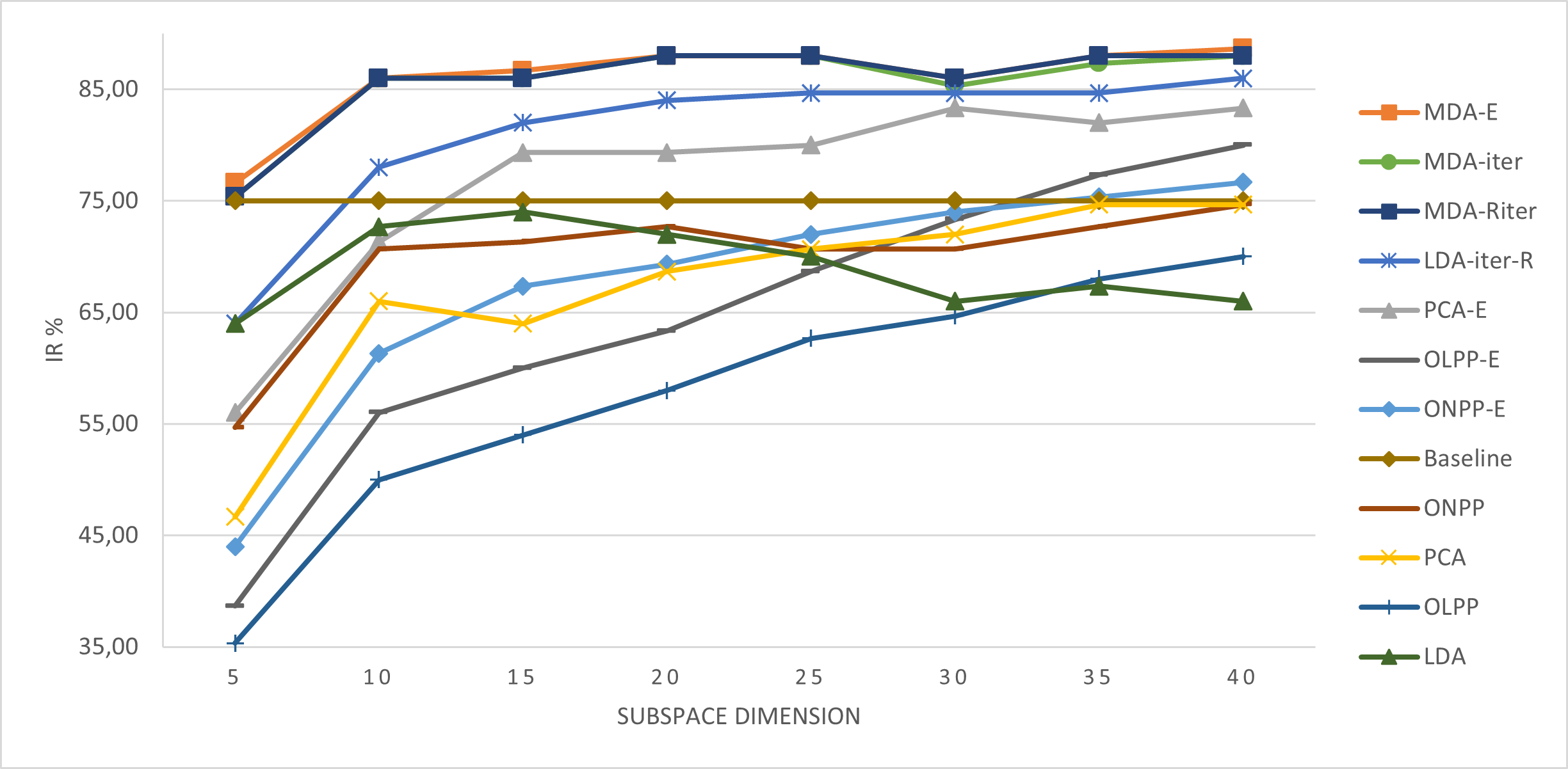
Figure 1: Performance of methods on the GTDB dataset, the names of methods on legend are ordered by their performance on dimension $d=40$.

	Baseline	$\bm{OLPP_{e}}$	$\bm{ONPP_{e}}$	$\bm{PCA_{e}}$	LDA	$\bm{MDA_{e}^{tr}}$	$\bm{MDA_{e}^{rt}}$	$\bm{MDA_{t}^{tr}}$
2	26.60	50.50	56.00	63.00	75.50	47.00	69.50	69.50
4	26.60	75.50	81.50	82.50	77.00	76.00	75.50	75.50
6	26.60	81.00	80.50	84.50	77.50	82.00	76.50	76.50
8	26.60	85.00	83.50	88.00	78.50	84.50	78.00	78.00
10	26.60	86.00	87.50	88.00	78.00	87.50	75.50	75.50

Table 2: Performance of methods per different subspace dimension on the DIV dataset.

The figure 1 shows the performance of the methods on the GTDB dataset. The results shows the superiority of the proposed method over the other methods, with a recognition rate big enough starting from $d=10$. It also shows the advantage in general of the high dimensional methods over the low dimensional ones, another observation is the regularization effect on LDA, is obvious compared to the MDA. The regularization is less effective in the high dimensional. Another observant, with the first figure, is the performance is noticeable in RGB images, which suggests that the methods are more effective when the data is in a higher dimensional.
The tables 1, 2 show the performance on the MNIST and DIV datasets, respectively. The results are consistent with the GTDB dataset, the proposed methods gains an improvement compared to the other methods.

	$\bm{MDA_{e}^{rt}}$	$\bm{MDA_{e}^{tr}}$	$\bm{LDA_{r}^{tr}}$	$\bm{MDA_{e}^{rt,ls}}$
5	57.05	482.66	16.06	23.07
10	50.46	423.79	16.28	22.79

Table 3: Time of different proposed methods on the GTDB dataset in seconds.

The table 3 shows the time of the methods on the GTDB dataset, notice that the dimension of the subspace does not affect the time, as the code pf methods use the function eig to compute the eigenvalues, then get only the number of dimensions that is wanted, instead of eigs that is quicker and gives the first $d$ eigenvalues directly.
The results confirms the theoretical complexity of the methods, as the iterative methods are slower, since they require the eigenvalue decomposition at each iteration (It is seen that 10 iterations is sufficient for the convergence for this data with the parameters mentioned before, which explains the 10 time slower for the iterative methods). It shows also a disadvantage of the high dimensional methods, as they require more time to compute the eigenvalues. It is interesting also to observe that Trace Ratio and Ratio Trace methods have the same performance, but with a different time, which can be a factor to choose between them.
It is clear that the results has an advantage on the cost of time complexity. It can well capture the low dimensional feature space.

6 Conclusion

In this paper, we have proposed a new method for dimensionality reduction and classification, called the Multilinear Discriminant Analysis via Einstein product (MDA-E). The method is based on the Trace Ratio problem, which aims to find a projection tensor that maximizes the between-class scatter tensor and minimizes the within-class scatter tensor. We have shown that the Trace Ratio problem has a unique solution up to a unitary transformation, and we have provided an iterative algorithm to solve it. We have also introduced a regularization term to ensure the existence of the solution. We have conducted experiments on the MNIST and GTDB and DIV datasets, comparing our method with state-of-the-art methods. The results show that our method outperforms the other methods, and is suitable when time is not a constraint. Future work will focus on improving the time complexity of the method, and on extending it to other applications.

7 Declaration of Competing Interest

The authors declare that they have no known competing financial interests or personal relationships that could have appeared to influence the work reported in this paper.

References

- [1] M. Bouallala, F. Dufrenois, K. Jbilou, and A. Ratnani, Trace ratio based manifold learning with tensor data, Numerical Linear Algebra with Applications, (2024), p. e2594.
- [2] M. Brazell, N. Li, C. Navasca, and C. Tamon, Solving multilinear systems via tensor inversion, SIAM Journal on Matrix Analysis and Applications, 34 (2013), pp. 542–570.
- [3] C. Chen, A. Surana, A. Bloch, and I. Rajapakse, Multilinear time invariant system theory, in 2019 Proceedings of the Conference on Control and its Applications, SIAM, 2019, pp. 118–125.
- [4] F. Dufrenois, A. El Ichi, and K. Jbilou, Multilinear discriminant analysis using tensor-tensor products, Journal of Mathematical Modeling, 11 (2023), pp. 83–101.
- [5] K. Fukunaga, Introduction to statistical pattern recognition, Elsevier, 2013.
- [6] J. Ji and Y. Wei, The drazin inverse of an even-order tensor and its application to singular tensor equations, Computers & Mathematics with Applications, 75 (2018), pp. 3402–3413.
- [7] E. Kokiopoulou and Y. Saad, Orthogonal neighborhood preserving projections: A projection-based dimensionality reduction technique, IEEE Transactions on Pattern Analysis and Machine Intelligence, 29 (2007), pp. 2143–2156.
- [8] E. Kokiopoulou and Y. Saad, Enhanced graph-based dimensionality reduction with repulsion laplaceans, Pattern Recognition, 42 (2009), pp. 2392–2402.
- [9] T. G. Kolda and B. W. Bader, Tensor decompositions and applications, SIAM review, 51 (2009), pp. 455–500.
- [10] K. Lee and J. Kim, On the equivalence of linear discriminant analysis and least squares, in Proceedings of the AAAI Conference on Artificial Intelligence, vol. 29, 2015.
- [11] S. Mika, G. Ratsch, J. Weston, B. Scholkopf, and K.-R. Mullers, Fisher discriminant analysis with kernels, in Neural networks for signal processing IX: Proceedings of the 1999 IEEE signal processing society workshop (cat. no. 98th8468), Ieee, 1999, pp. 41–48.
- [12] L. Qi and Z. Luo, Tensor analysis: spectral theory and special tensors, SIAM, 2017.
- [13] H. Wang, S. Yan, D. Xu, X. Tang, and T. Huang, Trace ratio vs. ratio trace for dimensionality reduction, in 2007 IEEE Conference on Computer Vision and Pattern Recognition, IEEE, 2007, pp. 1–8.
- [14] Y. Wang and Y. Wei, Generalized eigenvalue for even order tensors via einstein product and its applications in multilinear control systems, Computational and Applied Mathematics, 41 (2022), p. 419.
- [15] J. Ye, Least squares linear discriminant analysis, in Proceedings of the 24th international conference on Machine learning, 2007, pp. 1087–1093.
- [16] A. Zahir, K. Jbilou, and A. Ratnani, Multilinear algebra methods for higher-dimensional graphs, Applied Numerical Mathematics, (2023).
- [17] A. Zahir, K. Jbilou, and A. Ratnani, Higher order multi-dimension reduction methods via einstein-product, arXiv preprint arXiv:2403.18171, (2024).
- [18] A. Zahir, A. Ratnani, and K. Jbilou, Quaternion tensor low rank approximation, arXiv preprint arXiv:2409.10724, (2024).