Demystifying 5G Polar and LDPC Codes: A Comprehensive Review and Foundations

Abstract

This paper serves as a comprehensive guide for practitioners and scholars aiming to understand the channel coding and decoding schemes integral to the 5G NR standard, with a particular focus on LDPC and polar codes. We start by explaining the design procedures that underlie these channel codes, offering fundamental information from perspectives of both encoding and decoding. In order to determine the present status of research in this area, we also provide a thorough literature review. Notably, we add comprehensive, standard-specific information to these foundational evaluations that is frequently difficult to extract from technical specification documents. The significance of reviewing and refining the foundations of the aforementioned codes lies in their potential to serve as candidate error-correcting codes for the future 6G standard and beyond.

I Introduction

The Channel coding emerged when Shannon applied probability theory to the study of communication systems Shannon [1]. In his seminal work , Shannon demonstrated that errors introduced by a noisy channel can be reduced to a desired level through the use of an appropriate coding scheme, for a transmission rate that is less than or equal to the channel’s capacity. To optimize the performance of communication channels, various techniques can be employed to mitigate the effects of noise, disturbances, or distortions, while increasing the channel throughput until it approaches its maximum capacity. This can be achieved either by physically modifying the signal through modulation or by altering its content through channel coding. Most error-correcting codes are linear codes, which, due to their systematic representation, are classified as systematic codes. Linear block codes can be understood in a variety of ways, and some of the most commonly used in many contexts are Reed Solomon (RS) codes [2], Hamming codes [3], CRC codes, Bose–Chaudhuri–Hocquenghem (BCH) codes [4] and LDPC codes [5]. It is possible to represent a linear block code in matrix form or in the form of a graph factor.

• Generator Matrix: $\mathbf{G}$ is the generator matrix of dimension $\mathsf{K}\times\mathsf{N}$. The matrix is said to be systematic if $\mathbf{G}=[\mathbf{P}\ \mathbf{I}_{\mathsf{K}}]$ where $\mathbf{I}_{\mathsf{K}}$ and $\mathbf{P}$ is called the parity matrix of dimension ($\mathsf{K}\times\mathsf{N-K}$). In this case, the code is formed by parity bits followed by message bits.
  The matrix $\mathbf{G}$ is said to be non-systematic if $\mathbf{G}=[\mathbf{P}\ \mathbf{M}]$ where $\mathbf{M}$ is any matrix of size ($\mathsf{K}\times\mathsf{K}$).

• Parity Check Matrix: $\mathbf{H}$ is called the parity check matrix denoted as $\mathbf{H}=[\mathbf{I}_{\mathsf{N-K}}\ \mathbf{P}^{\mathsf{T}}]$, where $\mathbf{P}^{\mathsf{T}}$ is the transpose of the parity matrix $\mathbf{P}$. Thus, it can be easily shown that $\mathbf{G}\cdot\mathbf{H}^{\mathsf{T}}=\mathbf{0}$, where operations are performed in $\mathbb{F}_{2}$.

• Syndrome Checking: For each code word $\mathbf{c}$: $\mathbf{c}\cdot\mathbf{H}^{\mathsf{T}}=\mathbf{m}\cdot\mathbf{G}\cdot\mathbf{H}^{\mathsf{T}}=\mathbf{0}$, where $\mathbf{m}=[\mathrm{m}(0),\mathrm{m}(1),\ldots,\mathrm{m}(\mathsf{K}-1)]$. If $\mathbf{c}\cdot\mathbf{H}^{\mathsf{T}}\neq\mathbf{0}$, it means there are errors in the received bits.

In 5G NR, data and control streams from PHY to MAC layer are encoded /decoded to offer transport and control services over the radio transmission link. Channel coding scheme is a combination of error detection, error correcting, rate matching, interleaving and transport channel or control information mapping onto/splitting from physical channels.

Table I and Table II show the usage of coding scheme for the different types of Transport channels and for the different control information types [6].

TABLE I: Usage of channel coding scheme for transport channels (TrCHs). [6]

TrCH	Coding scheme
UL-SCH	LDPC
DL-SCH	LDPC
PCH	Polar code
BCH	Polar code

TABLE II: Usage of channel coding schemes within 5G NR UL/DL control channels [6].

Control Information	Coding scheme
DCI	Polar code
	Block code
UCI	Polar code

This paper serves as a guide and reference for both practitioners and scholars interested in understanding channel coding and decoding schemes, particularly the Low-Density Parity-Check (LDPC) and polar coding methods adopted in 5G and beyond, in line with 3GPP standard specifications. It highlights important information that can be difficult to extract from the technical specification documents established by the standard.

Notably, we enrich the foundational reviews of the main features of these two coding schemes with many standard-specific details, such as rate adaptation procedures, the application of Cyclic Redundancy Check (CRC), and aspects like decoding algorithms. The refinement and deeper understanding of these coding schemes are particularly relevant, as they are strong candidates for error correction in future 6G standards and beyond.

The article is structured as follows. Section II and Section III lays out the foundations and detailed reviews of 5G NR LDPC codes and 5G NR Polar codes respectively, Section IV presents the numerical results and performance analysis, and finally Section V concludes the paper.

Furthermore, the following is a list of acronyms that the reader will encounter throughout the manuscript:

5G

Fifth Generation of Wireless Cellular Technology

NR

New Radio

BCH

Broadcast Channel

BLER

Block Error Rate

BP

Belief Propagation

CA-SCL

CRC-aided Successive Cancellation List

CRC

Cyclic Redundancy Check

DCI

Downlink Control Information

DL-SCH

Downlink Shared Channel

ESC

Early Stop Criteria

LBP

Layered Belief Propagation

LDPC

Low-Density Parity-Check

LLR

Log-Likelihood Ratio

MAC

Medium Access Control

OFDM

Orthogonal Frequency Division Multiplexing

PCH

Paging Channel

PHY

Physical Layer

PUSCH

Physical Uplink Shared Channel

QPSK

Quadrature Phase Shift Keying

SC

Successive Cancellation

SCL

Successive Cancellation List

SNR

Signal-to-Noise Ratio

SU

Single User

TB

Transport Block

TDL

Tapped Delay Line

UCI

Uplink Control Information

UL-SCH

Uplink Shared Channel

URLLC

Ultra-Reliable-Low-Latency Communication

II 5G NR LDPC Codes

It is a curious twist of history that LDPC codes should have been largely unnoticed for so long. LDPC codes were originally proposed in 1962 by Gallager [5] . At that time, the codes might have been overlooked because contemporary investigations in concatenated coding overshadowed LDPC codes and because the hardware of the time could not support effective decoder implementations[7]. They therefore remained discrete until 1996 after the introduction of iterative decoding, initiated by the turbo codes[8]. Since then, LDPC codes have shown interesting performance and a relatively uncomplicated implementation. MacKay, working on Turbo codes at that time, gave a second birth to LDPC codes [9] and brings LDPC codes back into fashion. This article by Mackay presents constructions of LDPC codes and shows their good performance. Later, Luby, introduces irregular LDPC codes [10] characterized by a parity check matrix for which the distribution of the number of non-zero elements per row and/or column is not uniform. LDPC codes are linear block codes based on sparse parity-check matrix. It is forgotten for dozens of years because of the limited computation ability. In recent years, LDPC codes attract more attention because of their efficient decoding algorithms, excellent error-correcting capability, and their performance close to the Shannon limit for large code lengths. LDPC coding is currently adopted in 5G NR for both uplink and downlink shared transport channels. Given that 5G must support high data rates of up to 20 Gbps and a wide range of block sizes with different coding rates for data channels and hybrid automatic repeat request (HARQ), LDPC codes are a de facto candidate to meet these requirements. Indeed, the base graphs defined in 3GPP TS 38.212 [6] are structured parity-check matrix, which can efficiently support HARQ and rate compatibility that can support arbitrary amount of transmitted information bits with variable code rates. While Polar codes are applied to 5G NR control channels, LDPC codes are suitable for 5G NR shared channels due to its high throughput, low latency, low decoding complexity and rate compatibility. Another advantage of the NR 5G codes is that the performance of the LDPC codes has an error floor around or below the $10^{5}$ BLER for all code width and code rates, making LDPC codes, an essential channel coding scheme for URLLC application scenarios.

II-A State-of-art LDPC codes

In reviewing the literature, significant efforts have been directed towards enhancing the error correction performance of 5G communication systems. The discourse surrounding channel coding in cellular systems, particularly for 5G, initially emphasized turbo, LDPC, and polar codes, with LDPC codes adopted for eMBB data and polar codes for control [11]. In this regard, Srisupha et al. [12] developed an experimental kit demonstrating LDPC encoding processes, emphasizing flexibility between software and hardware LDPC encoders. Subsequently, Belhadj et al. [13] compared error correction performance between LDPC and polar codes in 5G machine-to-machine (M2M) communications, highlighting specific requirements for different M2M applications. Later on, Li et al. [14] proposed dynamic scheduling strategies to reduce decoding complexity and improve error correction performance for short LDPC codes. Next, in a perspective of accelerated LDPC decoding, Tian and Wang [15] presented a base graph-based static scheduling method for layered decoding of 5G LDPC codes, achieving notable reductions in iteration numbers and performance enhancements. In [16, 17], authors investigated the structure and features of the base graphs [6], showing that the usage of a circularly shifted identity matrix known as the permutation matrix can greatly reduce the memory requirement for implementation. Indeed, 5G LDPC base graphs design aims to provide row orthogonality for fast and reliable decoding. Row orthogonality in 5G LDPC base graphs design can somehow reduce decoding latency. Both base graphs and all code rates involve puncturing code bits associated with the first two circulant columns prior to transmission, targeting high-weight columns for performance enhancement. Therefore, puncturing serves as a means of improving overall system performance [17]. Additionally, 5G LDPC fully utilizes the double diagonal structure of the base graphs. Due to the characteristic of base graphs, the double-diagonal structure can make LDPC encoding more efficient. Conversely, [18] proposed a novel efficient encoding method and a high-throughput low-complexity encoder architecture for 5G NR LDPC.

Furthermore, efforts have been directed towards optimizing implementations of these codes for heightened performance on software and hardware targets. For instance, Liao et al. [19] present a high-throughput LDPC encoding on a single graphics processing unit (GPU), while Tarver et al. [20] explore GPU-based LDPC decoding, showcasing potential for high throughput and low latency applications in 5G and beyond. Additionally, hardware architectures have been developed to efficiently decode LDPC codes, as seen in the work of Nadal and Baghdadi [21], who propose a highly parallel field-programmable gate array (FPGA) architecture. Conversely, Xu et al. [22] focus on software decoding with SIMD acceleration on Intel Xeon CPUs, achieving notable throughput with low latency. Sy [23] proposed optimisation strategies for low-latency 5G LDPC decoding over GPPs. Meanwhile, Li et al. [24] addressed the challenge of achieving high throughput rates, proposing a multicore LDPC decoder architecture achieving up to 1 Tb/s throughput for beyond 5G systems, while Aronov et al. [25] compare LDPC decoding performance between GPU and FPGA platforms, stressing the need for further optimization, particularly in reducing latency for GPU-based solutions.

Moreover, the selection of coding schemes for 5G eMBB services has been a focus of interest, with quasi-cyclic LDPC and polar codes chosen for data and control channels, respectively. Rao and Babu. [26] highlighted the importance of these codes, particularly QC-LDPC, and Wu et al. [27] proposed an efficient QC-LDPC implementation for 5G NR, enhancing throughput by matrix pruning. Ivanov et al. [28] introduced a novel concatenated code construction comprising outer and inner LDPC codes, demonstrating reduced decoding complexity and superior performance. Additionally, Song et al. [29] emphasized the significance of well-designed LDPC codes, particularly QC-LDPC codes, in approaching channel capacity and enabling high-speed data transmission. In parallel, LDPC codes’ adoption in 5G standards underscores their importance in broadcasting and cellular communication systems Ahn et al. [30]. Moreover, Cui et al. [31] tackled the challenge of designing high-performance and area-efficient decoders, while Trung et al. [32] and Jayawickrama and He [33] proposed adaptations and improved algorithms for LDPC decoding in 5G NR. Additionally, Li et al. [34] focused on LDPC code design for specific 5G scenarios, proposing optimization methods and an improved decoding algorithm. Wu and Wang [35] provided insights into LDPC decoding latency in 5G NR, guiding decoder design to meet high throughput and low latency requirements. In Sun and Jiang. [36] proposed a hybrid decoding algorithm for LDPC codes in 5G, where normalized min-sum algorithm (NMSA) decoding and linear approximation are combined, with only a slight increase in complexity for NMSA and an improved performance much closer to belief propagation BP decoding, especially for low-rate codes.

Recently, there has been a growing interest in applying deep learning techniques to various aspects of 5G communications, as reviewed by Dai et al. [37]. Shah and Vasavada [38] proposed normalized least-mean-square (NLMS) algorithms to enhance the decoding performance of 5G LDPC codes, leveraging deep neural networks (DNNs) to optimize parameters. Tang et al. [39] introduced a scheme combining model-driven deep learning with traditional BP decoding algorithms to adapt LDPC codes for different 5G scenarios. Lastly, Andreev et al. [40] investigated the application of DNNs to improve the decoding algorithms of short QC-LDPC codes in the 5G standard, addressing the curse of dimensionality problem and enhancing performance.

II-B Foundations and Fundamentals

The LDPC code is presented in matrix form $[\mathbf{G},\mathbf{H}]$, where $\mathbf{G}$ is the generator matrix of the code and $\mathbf{H}$ is the parity check matrix (PCM). The parity matrix $\mathbf{H}$ is sparse, containing very few ones. It can be represented in the form of a Tanner graph. This graph consists of two types of nodes: bit nodes (BNs) and check nodes (CNs) which are connected by edges. The BNs and CNs correspond, respectively, to the columns (code word bits) and rows (parity constraints) of the matrix $\mathbf{H}$. A variable node $i$ is connected to a check node $j$ if $\mathbf{H}(i;j)=1$. This graph is bipartite, since nodes of the same type cannot be connected (i.e., a CN cannot be connected to another CN). Tanner graphs are commonly used to represent the parity matrix in LDPC codes. A Tanner graph leads to decoding algorithms of fairly low complexity [7].

$$\mathbf{H}=\left[\begin{array}[]{llllllll}0&1&0&1&1&0&0&1\\ 1&1&1&0&0&1&0&0\\ 0&0&1&0&0&1&1&1\\ 1&0&0&1&1&0&1&0\end{array}\right]$$ (1)

The number of variable nodes equals the number of received bits ($N$), which is equivalent to the number of columns in the matrix $\mathbf{H}$. Similarly, the number of parity check nodes corresponds to the number of rows $(\mathsf{N}-\mathsf{K})$ in the matrix $\mathbf{H}$.

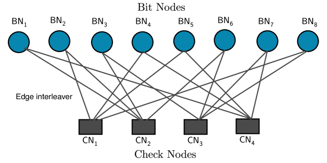
Figure 1: Parity check matrix $\mathbf{H}(4,8)$ and the corresponding Tanner graph.

The most important element in the realization of a good LDPC code is the $\mathbf{H}$ matrix which will condition the quality of the iterative decoding. There are four important parameters to respect in order to obtain a good $\mathbf{H}$ parity check matrix.

1. Code Rate. We can increase the rate of an LDPC code by adding 1s in the lines of the Matrix $\mathbf{H}$.

   If the parity matrix is regular, it can also be denoted ($\mathrm{N}$, $w_{c}$, $w_{d}$), where $w_{b}$ represents the weight of a row and $w_{b}$ represents the weight of a column. The yield can be calculated as a function of $w_{c}$ and $w_{b}$ by $\mathrm{R}=1-w_{b}/w_{c}$

2. short cycles (girth). The generation of short cycles in the equivalent Tanner graph of the code must be avoided. A cycle represents from a given variable node the set of parity and variable nodes that will be connected to it until we fall back on the starting variable node. We call girth the minimum cycle length that can be encountered in a Tanner graph. Short cycles are very penalizing because they involve few intermediate nodes, and thus the extrinsic information they generate during decoding becomes quickly and strongly correlated.

3. Size of $\mathbf{H}$. A large matrix allows better coding Rate and consequently better performance.

4. Construction algorithm of $\mathbf{H}$. To construct the regular parity matrix, there are mainly two methods: the random method and the deterministic method. The most known random methods in the literature for the construction of the $\mathbf{H}$-matrix are the Gallager method [5] and the progressive Edge Growth (PEG) method [41] which makes it possible to create graphs with large girths. For the deterministic method, the most used is the Quasi-cyclic method. The latter uses a deterministic construction based on a circular permutation of the identity matrix [27, 42]. QC-LDPC codes belong to the class of structured codes that are relatively easier to implement without significantly compromising the performance of the code. Well-designed QC-LDPC codes have been shown to outperform computer-generated random LDPC codes, in terms of bit-error rate and block-error rate performance and the error floor. These codes also offer merits in decoder hardware implementation due to their cyclic symmetry, which results in simple regular interconnection and modular structure[43].

II-C 3GPP 5G LDPC Codes

NR LDPC code is a family of QC-LDPC codes. It is constructed from a matrix named $\mathbf{H}_{\mathsf{BG}}$ of dimension $M\times N$ called base graph matrix $\mathbf{BG}$. The $\mathbf{H}_{\mathsf{BG}}$ matrices are selected in the 5G NR coding process according to the coding rate and the length of the transport block or code block. Thus, for $\mathbf{BG}_{\mathsf{1}}$ ($N=68$, $M=46$) and for $\mathbf{BG}_{\mathsf{2}}$ ($N=52$, $M=42$). Since $\mathbf{BG}_{\mathsf{1}}$ is targeted for larger block length $\mathsf{K}\leq 8448$ and coding rates between $1/3\leq\mathrm{R}\leq 8/9$, $\mathbf{BG}_{\mathsf{2}}$ is employed for small blocks $\mathsf{K}\leq 3840$ and coding rates between $1/5\leq\mathrm{R}\leq 2/3$.

For $\mathbf{BG}_{\mathsf{1}}$, $\mathrm{K}=22\mathrm{Z_{c}}$ and for $\mathbf{BG}_{\mathsf{2}}$, $\mathrm{K}=10\mathrm{Z_{c}}$, where $\mathsf{K}$ is the maximum number of information bits, and $\mathrm{Z_{c}}$ is the lifting size shown in Table III. There are 51 lifting sizes from 2 to 384 for each base graph. Both $\mathbf{BG}_{\mathsf{1}}$ and $\mathbf{BG}_{\mathsf{2}}$ have the same block structure. The columns include information columns, core parity columns, and extension parity columns. The rows are divided into core check rows and extension check rows.

For $\mathbf{BG}_{\mathsf{1}}$, $\mathbf{A}$ is a $4\times 22$ matrix; $\mathbf{A}$ is a $4\times 4$ matrix; $\mathbf{O}$ is $4\times 42$ all zero matrix; $\mathbf{B}$ is a $42\times 22$ matrix; $\mathbf{C}$ is a $42\times 4$ matrix; $\mathbf{I}$ is $42\times 42$ identity matrix;
For $\mathbf{BG}_{\mathsf{1}}$, $\mathbf{A}$ is a $4\times 10$ matrix; $\mathbf{E}$ is a $4\times 4$ matrix; $0$ is $4\times 38$ all zero matrix; $\mathbf{B}$ is a $38\times 10$ matrix; $\mathbf{C}$ is a $38\times 4$ matrix; $\mathbf{I}$ is $38\times 38$ identity matrix; Sub-matrix $\mathbf{E}$ is a double diagonal matrix that is benefit for encoding. An example of $\mathbf{BG}_{\mathsf{1}}$ with set index of listing size (iLS) =$1$ in 3GPP TS 38.212[6] standard is shown in Figure 2. In order to distinguish with the number $1$ in base graphs in 3GPP TS 38.212 [6] standard, null value in the base graph will be replaced by $-1$.

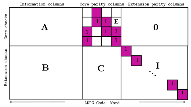
Figure 2: 3GPP NR Base graphs structure.

In 3GPP TS 38.212 [6] standard, the maximum lifting size value for each set of iLS is shown in Table III. The value of each element $\mathsf{p_{i,j}}$ also known as the circular shift value is from -1 to 383, which is a property of the $\mathbf{BG}$s.

TABLE III: Sets of LDPC lifting size [6]

Set index (iLS)	Set of lifting sizes (Z)
0	2, 4, 8, 16, 32, 64, 128, 256
1	3, 6, 12, 24, 48, 96, 192, 384
2	5, 10, 20, 40, 80, 160, 320
3	7, 14, 28, 56, 112, 224
4	9, 18, 36, 72, 144, 288
5	11, 22, 44, 88, 176, 352
6	13, 26, 52, 104, 208
7	15, 30, 60, 120, 240

NR LDPC codes also offer an additional coding advantage at lower code rates, rendering them suitable for scenarios requiring high reliability. Regarding decoding complexity, opting for $\mathbf{BG}_{\mathsf{2}}$ proves advantageous due to its compactness and utilization of a larger lifting size element, translating to enhanced parallelism compared to $\mathbf{BG}_{\mathsf{1}}$. The decoding latency tends to correlate with the number of non-zero elements in the base graph, with $\mathbf{BG}_{\mathsf{2}}$ exhibiting significantly lower latency than $\mathbf{BG}_{\mathsf{1}}$ for a given code rate, owing to its fewer non-zero elements [43].
Furthermore, the parity-check matrix $\mathbf{H}$ is obtained by replacing each element of the base graph $\mathbf{H}_{\mathsf{BG}}$ with a $\mathrm{Z_{c}}\times\mathrm{Z_{c}}$ matrix, according to the following rules.

• Each element of value $-1$ in $\mathbf{H}_{\mathsf{BG}}$ is replaced by a null matrix of size $\mathrm{Z_{c}}\times\mathrm{Z_{c}}$.

• Each element of value $0$ in $\mathbf{H}_{\mathsf{BG}}$ is replaced by an identity matrix $\mathbf{I}$ of size $\mathrm{Z_{c}}\times\mathrm{Z_{c}}$.

• Each element of value from 1 to $\mathrm{Z_{c}}-1$ in $\mathbf{H}_{\mathsf{BG}}$ which is denoted by $\mathsf{p_{i,j}}$ is replaced by a circular permutation matrix $\mathbf{I}(\mathsf{p_{i,j}})$ of size $\mathrm{Z_{c}}\times\mathrm{Z_{c}}$, where $i$ and $j$ are the row and column indices of the element, and $\mathbf{I}(\mathsf{p_{i,j}})$ is obtained by circularly shifting the identity matrix $\mathbf{I}$ of size $\mathrm{Z_{c}}\times\mathrm{Z_{c}}$ to the right $\mathsf{p_{i,j}}$ times [6].

The main advantage of using a circularly shifting identity matrix is that it can reduce the memory requirement for implementation [17].
To simplify, a small example can be used to explain the principle of obtaining the parity check matrix $\mathbf{H}$. Hence, assuming that $\mathbf{H}_{\mathsf{{BG}}}$ is a given base graph matrix with lifting size $\mathrm{Z_{c}}$=4,

$$\mathbf{H}_{\mathsf{BG}}=\left[\begin{array}[]{cccccc}{\color[rgb]{0,1,1}2}&{\color[rgb]{.5,0,.5}-1}&{\color[rgb]{1,.5,0}1}&{\color[rgb]{.75,.5,.25}3}&{\color[rgb]{0,1,0}0}&{\color[rgb]{.5,0,.5}-1}\\ {\color[rgb]{1,.5,0}1}&{\color[rgb]{0,1,0}0}&{\color[rgb]{.5,0,.5}-1}&{\color[rgb]{0,1,0}0}&{\color[rgb]{0,1,0}0}&{\color[rgb]{0,1,0}0}\\ {\color[rgb]{.5,0,.5}-1}&{\color[rgb]{.75,.5,.25}3}&{\color[rgb]{0,1,1}2}&{\color[rgb]{1,.5,0}1}&{\color[rgb]{.5,0,.5}-1}&{\color[rgb]{0,1,0}0}\end{array}\right],$$ (2)

the corresponding parity check matrix $\mathbf{H}$ is shown to be:

$$\includegraphics[width=346.89731pt]{Figures/ldpc/H-MATRIX.pdf}.$$ (3)

The overall LDPC transmission chain from MAC/PHY layer processing schematic is depicted in Figure 3, which describes the transmit-end for the PUSCH/PDSCH supporting a transport block CRC attachment, LDPC base graph selection, code block segmentation and code block CRC attachment, LDPC encoding, rate matching code block concatenation. The receiver end is therefore the transmitter end in the reverse flow.

(a) Transmitter end.

(b) Receiver end.

Figure 3: Conceptual illustration of 5G LDPC transceiver chain.

At the transmitter end, we can list the following components.

1. Transport block CRC attachment.
   CRC is an error detection code used to measure BLER after decoding. The entire transport block is used to calculate CRC parity bits. Assume that the transport message before CRC attachment is $a(0),a(1),\ldots,a(A-1)$, where A is the size of the transport block message. Parity bits are $p(0),p(1),\ldots,p(L-1)$, where $L$ is the number of parity bits. The parity bits are generated by one of the following cyclic generator polynomials[6]. if $A>3824$, the generator polynomial $\mathrm{g}_{\mathsf{CRC24A}}(\beta)$ is used.

   $$\begin{array}[]{r}\mathrm{g}_{\mathsf{CRC24A}}(\beta)=\left[\beta^{24}+\beta^{23}+\beta^{18}+\beta^{17}+\beta^{14}+\beta^{11}+\beta^{10}\right.\\ \left.+\beta^{7}+\beta^{6}+\beta^{5}+\beta^{4}+\beta^{3}+\beta+1\right].\end{array}$$ (4)

   The length of parity bits $L=24$. Otherwise, the generator polynomial $\mathbf{g}_{CRC16}(\beta)$ is used.

   $$\mathrm{g}_{\mathsf{CRC16}}(\beta)=\left[\beta^{16}+\beta^{12}+\beta^{5}+1\right].$$ (5)

   The length of parity bits $L=16$. The message bits after attaching CRC are $b(1),b(2),\ldots,b(B)$, $B$ represents the transport block information size with CRC bits such that $B=A+L$.
   

   $$b_{k}=\left\{\begin{array}[]{ll}a_{k},&\texttt{ \footnotesize{for} }k=0,1,\ldots,A-1\\ p_{k-A},&\texttt{ \footnotesize{for} }k=A,A+1,\ldots,A+L-1.\end{array}\right.$$ (6)

   The CRC value was determined to satisfy the probability of misdetection of the TB with BLER $\sim$ $10^{6}$ as well as the inherent error detection of LDPC code.

2. LDPC base graph selection.
   LDPC $\mathbf{BG}$ is selected based on the transport block message size $A$ and transport block coding rate $\mathrm{R}$. If $A\leq 292$, or if $A\leq 3824$ and $\mathrm{R}\leq 0.67$, or if $\mathrm{R}\leq 0.25$, LDPC $\mathbf{BG}_{\mathsf{2}}$ is used. Otherwise, LDPC $\mathbf{BG}_{\mathsf{1}}$ is used [6].

3. Code block segmentation and code block CRC attachment.
   The input message to CB segmentation is a transport message with CRC, denoted as $b(1),b(2),\ldots,b(B)$, where $B$ is the input message length. Assume that the maximum code block length is $\mathsf{K}_{cb}$, where $\mathsf{K}_{cb}=8448$ for $\mathbf{BG}_{\mathsf{1}}$ and $\mathsf{K}_{cb}=3840$ for $\mathbf{BG}_{\mathsf{2}}$. Code block segmentation is based on the following rules.
   Assume that $C$ is the number of code blocks.
   if $B\leq\mathsf{K}_{cb}$,

   $$C=1,\quad L=0,\quad B_{r}=B.$$ (7)

   Otherwise,

   $$C=\left[B/\left(\mathsf{K}_{cb}-L\right)\right],\quad L=24,\quad B_{r}=B+C\cdot L.$$ (8)

   Assume that the output of code block segmentation is $c_{r}(0),c_{r}(1),\ldots,c_{r}(\mathrm{K}_{r}-1)$, $\mathrm{K}_{r}=\mathrm{K}$ is the number of bits for the $r$-th code block. For $\mathbf{BG}_{\mathsf{1}}$, $\mathrm{K}=22\mathrm{Z_{c}}$ and for $\mathbf{BG}_{\mathsf{2}}$, $\mathrm{K}=10\mathrm{Z_{c}}$, where $\mathrm{Z_{c}}$ is a lifting size that is the minimum value of $\mathrm{Z_{c}}$ in all sets of lifting sizes in Table III which can meet formula (9).

   $$\mathsf{K}_{b}\cdot\mathrm{Z_{c}}\geq\mathrm{K}_{r}$$ (9)

   Where $\mathrm{K}_{r}$ is the number of information and CRC bits in a code block and $\mathrm{K}_{r}=B_{r}/C$. $\mathsf{K}_{b}$ is related with LDPC base graph type and the size of input message $B$, shown in Table IV.

   TABLE IV: $\mathsf{K}_{b}$ value [[6]

   $\mathbf{BG}$	$B$	$\mathsf{K}_{b}$
   1	all	22
   2	$B$ $>$ 640	10
   2	560 $<$ $B$ $\leq$ 640	9
   2	192 $<$ $B$ $\leq$ 560	8
   2	$B$ $\leq$192	6

   The output of code block segmentation $c_{r,k}$ is calculated as following,
   If $C=1$,

   $$c_{r,k}=\left\{\begin{array}[]{l l}b_{k},&\texttt{ \footnotesize{for} }1\leq k\leq B\\ \texttt{NULL},&\texttt{ \footnotesize{for} }B+1\leq k\leq\mathrm{K}.\end{array}\right.$$ (10)

   If $C>1$, block code should be attached CRC using the generator polynomial $\mathrm{g}_{\mathsf{CRC24B}}(\beta)$, the length of parity bits $L=24$.

   $$\mathrm{g}_{\mathsf{CRC24B}}(\beta)=\left[\beta^{24}+\beta^{23}+\beta^{6}+\beta+1\right].$$ (11)

   Assume that CRC parity bits are $p_{r}(1),p_{r}(2),\ldots,p_{r}(L)$,

   $$c_{r,k}=\left\{\begin{array}[]{ll}b_{k},&\texttt{ \footnotesize{for} }1\leq k\leq\mathrm{K}_{r}-\mathrm{L}\\ p_{r\left(k+L-\mathrm{K}_{r}\right)},&\texttt{ \footnotesize{for} }\mathrm{K}_{r}-\mathrm{L}+1\leq k\leq\mathrm{K}_{r}\\ \texttt{NULL},&\texttt{ \footnotesize{for} }\mathrm{K}_{r}+1\leq k\leq\mathrm{K},\end{array}\right.$$ (12)

   where $1\leq r\leq C$ and $\mathrm{K}$ is the maximum number of information bits for base graphs.

4. LDPC encoding.
   Each CB message is encoded independently. The input bit sequence in a CB to be passed to the LDPC encoder can be represented as $\mathbf{c}_{r}=[c_{r}(0),c_{r}(1),\ldots,c_{r}(\mathrm{K}_{r}-1)]^{\mathsf{T}}$, where $\mathrm{K}_{r}$ is the number of information bits within a CB to encode, the redundant bits are called parity bits denoted by $\mathbf{w}=[w(0),w(1),\ldots,w(\mathrm{N}_{r}+2\mathrm{Z_{c}}-\mathrm{K}_{r}-1)]^{\mathsf{T}}$. The output LDPC coded bits are denoted by $d_{r}(0),d_{r}(1),\ldots,d_{r}(\mathrm{N}_{r}-1)$ where $\mathrm{N}_{r}=66\mathrm{Z_{c}}$ for $\mathbf{BG}_{\mathsf{1}}$ and $\mathrm{N}_{r}=50\mathrm{Z_{c}}$ for $\mathbf{BG}_{\mathsf{2}}$, where the value of lifting factor $\mathrm{Z_{c}}$ is given in Table III. The LDPC encoding is based on the following procedure [6].

   1. Find the set with index iLS in Table III which contains $\mathrm{Z_{c}}$.

   2. Set $d_{r,{k-2\mathrm{Z_{c}}}}=c_{k},\forall k=2\mathrm{Z_{c}},\ldots,\mathrm{K}_{r}-1$.

   3. Generate $\mathrm{N}_{r}+2\mathrm{Z_{c}}-\mathrm{K}_{r}$ parity bits $\mathbf{w}=[w(0),w(1),\ldots,w(\mathrm{N}_{r}+2\mathrm{Z_{c}}-\mathrm{K}_{r}-1)]^{\mathsf{T}}$ such that $\mathbf{H}\times\left[\mathbf{c}_{r}\ \mathbf{w}\right]^{\mathsf{T}}=\mathbf{\mathbf{0}}$.

   4. The encoding is performed in $\mathbb{F}_{2}$.

   5. Set $d_{r,{k-2\mathrm{Z_{c}}}}=w_{k-\mathrm{K}_{r}},\forall k=\mathrm{K_{r}},\ldots,\mathrm{N}_{r}+2\mathrm{Z_{c}}-1$.

5. Rate matching:
   The rate matching aims to adapt different code rates. Rate matching is based on redundancy version (RV) from 0 to 3 [6]. Each RV divides the base graph, excluding the first two columns, into four chunks at different positions. Note that the first two columns are always punctured to improve performance. RV $0$ is well suited for the first transmission and has good self-decodability [44].

   Hence, the rate matching is carried out on each code block independently. Assume that the coded message bit output from the LDPC encoder of the $r-th$ code block is $d_{r}(1),d_{r}(2),\ldots,d_{r}(\mathrm{N}_{r})$ and $E_{r}$ is the length of the output message after performing rate matching on this $r-th$ coded message. Thus, the output bit-message from the rate matcher is denoted by $e_{r}(1),e_{r}(2),\ldots,e_{r}(E_{r})$ which is calculated using the following equation:

   $$e_{r,k}=d_{r,k},\texttt{\footnotesize{ if }}d_{r,k}\neq\texttt{NULL},\texttt{\footnotesize{ where }}1\leq k\leq E_{r}.$$ (13)

6. Code block concatenation:
   The CB concatenation aims to concatenate all code blocks message to a sequence of transport block message, which will be transmitted through the physical channel. Assume that the output message of code block concatenation is $g(1),g(2),\ldots,g(G)$, where $G$ is the desired length of the message of the transport block.

   $$g_{\ell}=e_{r,k},\texttt{\footnotesize{ where }}1\leq\ell\leq G,\quad 1\leq k\leq E_{r}.$$ (14)

Conversely, the receiver counterpart, is simply the reverse flow of the transmitter, and set out as follows :

1. Code block de-concatenation.
   The CB de-concatenation is used to break the transport block message into C numbers of code blocks message. Assume that the input message to code block de-concatenation is $y(0),y(1),\ldots,y(G-1)$. The output message from code block de-concatenation is $f_{r}(0),f_{r}(1),\ldots,f_{r}(E_{r}-1)$ .

   $$f_{r,k}=y_{\ell},\texttt{\footnotesize{ where }}1\leq\ell\leq G,\quad 1\leq k\leq E_{r}.$$ (15)

2. Rate de-matching.
   The rate de-matching aims to covert the code block message to the format that can be used for 5G LDPC parity-check matrix to process decoding. Rate de-matching is done on each code block independently. Assume that the input message is $f_{r}(0),f_{r}(1),\ldots,f_{r}(E_{r}-1)$. The output message from rate de-matching is $g(0),g(1),\ldots,g(N_{r}+2\mathrm{Z_{c}}-1)$

   $$g_{k}=\left\{\begin{array}[]{ll}0,&\texttt{ \footnotesize{for} }1\leq k\leq 2\mathrm{Z_{c}},\\ f_{k},&\texttt{ \footnotesize{for} }2\mathrm{Z_{c}}+1\leq k\leq E_{r},\\ 0,&\texttt{ \footnotesize{for} }E_{r}+1\leq k\leq\mathrm{N}+2\mathrm{Z_{c}}.\end{array}\right.$$ (16)

3. LDPC decoding.
   The LDPC decoding is done on each code block independently, and many decoding algorithms can be used. Subsection II-D highlights different LDPC decoding algorithms.

4. Code block de-segmentation. The CB de-segmentation is used to extract the message bits and transport block attached CRC bits. Assume that the output from code block de-segmentation is $\hat{b}(0),\hat{b}(1),\ldots,\hat{b}(B-1)$, where $B$ is the size of original transport block information with attached CRC bits. The input to the code block de- segmentation is $h_{r}(0),h_{r}(1),\ldots,h_{r}(\mathrm{N}+2\mathrm{Z_{c}}-1)$

   $$\hat{b}_{k}=h_{r,s},\texttt{\footnotesize{ where }}1\leq k\leq B,\quad 1\leq s\leq\mathrm{K}_{r}-L.$$ (17)

   $\mathrm{K}_{r}$ is the number of information and CRC bits in a code block and $L$ is the length of CRC bits in a code block.

5. CRC check:
   The CRC detachment is used to extract the CRC bits in transport block after the information transmitted in 5G NR shared channels. Then the extracted CRC bits will be checked with the original CRC bits attached to transport block information before transmitted.

II-D Soft-Decision based LDPC decoding Algorithms

The optimal performing method is soft-decision decoding, involving the computation of log-likelihood ratios (LLRs) and the exchange of extrinsic information between variable and parity nodes. This method is known by various names in the literature, such as the belief propagation algorithm (BPA), or message massing algorithm (MPA), or sum product (SPA) algorithm. Additionally, there is the min-sum algorithm(MSA), an approximate method with lower complexity compared to SPA. Various algorithmic variants are available, tailored to specific practical applications and necessitating simplifications for tractable implementation.

The message passing decoding can be divided into bit or variable nodes’ operation, also called row operation, and check nodes’ operation, also called column operation. A MPA based on Pearl’s belief algorithm describes the iterative decoding steps. The message probability passed between check nodes and variable nodes can be called belief, such as $\mathrm{q}_{ij}$ and $\mathrm{r}_{ji}$ in Figures 4 and 5.

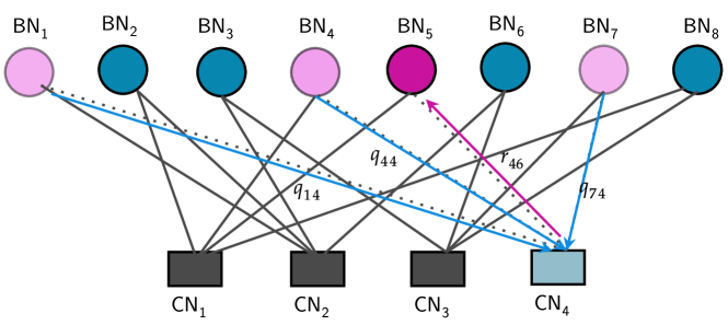
Figure 4: Check Node Updates: $\mathsf{CN}_{4}\longrightarrow\mathsf{BN}_{5}$ .

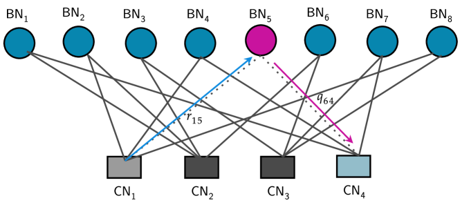
Figure 5: Bit Node Updates: $\mathsf{BN}_{5}\longrightarrow\mathsf{CN}_{4}$.

Index sets $\mathsf{BN}_{j\backslash i}$ and $\mathsf{CN}_{i\backslash j}$ are based on the parity check matrix (PCM). Index set $\mathsf{CN_{i}}$ and $\mathsf{BN_{j}}$ correspond to all non-zero element on column $i$ and row $j$ of the PCM, respectively. Figure 6 a simple conceptual illustration of BN and CN index sets within the PCM provided in (1) for the specified values of $i=3$ and $j=2$.

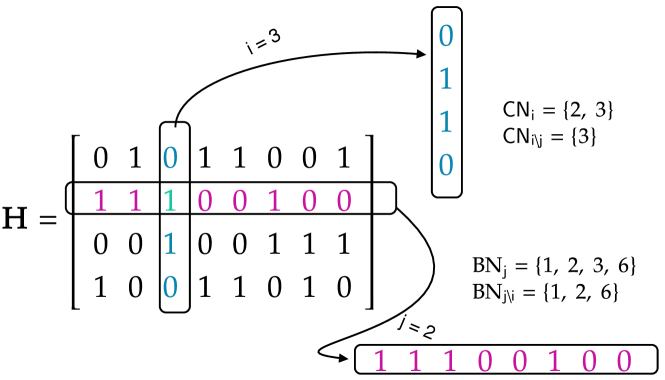
Figure 6: Conceptual Illustration of CNs and BNs processing Within BN and CN index sets for the specified values of $i$ and $j$.

Furthermore, the beliefs can be described via the following equations. Assume that a sequence of information bits are independently $\mathbf{c}=[\mathrm{c}(0),\mathrm{c}(1),\ldots,\mathrm{c}(\mathrm{N}-1)]$.

and consider the following notation :

• $\mathsf{BN}_{j}$ = Bit nodes connected to check node $j$,

• $\mathsf{BN}_{j\backslash i}$ =bit nodes connected to check node $j$, excluding bit node $i$,

• $\mathsf{CN}_{i}$ = check nodes connected to variable node $i$,

• $\mathsf{CN}_{i\backslash j}$ =check nodes connected to bit node $i$, excluding check node $j$,

• $p_{i}=p_{r}(\mathrm{c}_{i}=1|\mathrm{y}_{i})$ , is the probability of $\mathrm{c}_{k}$ = 1.

• $\mathrm{y}_{i}$ is the channel sample at variable node $i$.

• The check-to-variable extrinsic message passing to the $j-th$ variable node from the $i-th$ check node is denoted by $\mathscr{L}\left(\mathrm{r}_{ji}\right)$ and $\mathscr{L}\left(\mathrm{q}_{ij}\right)$ is the variable-to-check extrinsic message.

The belief propagation algorithm is adaptable to representation in both probability and log domains, wherein probabilities are expressed as LLRs. Employing LLR domain decoding offers a reduction in implementation complexity, since multiplications in the probability domain can be equivalently represented as additions in the log domain. Besides, many multiplications of probabilities involved could become numerically unstable, so the log domain algorithm is preferred [7].

1) Sum Product Algorithm (SPA)

The Sum Product Algorithm, also known as (BPA), constitutes a fundamental soft decision decoding approach where messages are conveyed as probabilities. The implementation of Belief Propagation relies on the decoding algorithm introduced by Gallager [5]. For a transmitted LDPC encoded codeword, $\mathbf{c}$, the input to the LDPC decoder is the LLR value defined as follows :

$$\mathscr{L}\left(\mathrm{c}_{i}\right)=\log\frac{p_{r}\left(\mathrm{c}_{i}=0\mid\texttt{\footnotesize{channel output for}}\ \mathrm{c}_{i}\right)}{p_{r}\left(\mathrm{c}_{i}=1\mid\texttt{\footnotesize{channel output for}}\ \mathrm{c}_{i}\right)}.$$ (18)

In each iteration, the algorithm updates its key components through horizontal and vertical processing steps.

The check nodes to bit nodes operation (horizontal processing ) is based on (19).

$$\mathscr{L}\left(\mathrm{r}_{ji}\right)=\log\frac{\mathrm{r}_{ji}(0)}{\mathrm{r}_{ji}(1)}$$ (19)

$$=2\tanh^{-1}\left(\prod_{i^{\prime}\in\mathsf{BN}_{j\backslash i}}\tanh\left(\frac{1}{2}\mathscr{L}\left(\mathrm{q}_{i^{\prime}j}\right)\right)\right),$$

$$=\left(\prod_{i^{\prime}\in\mathsf{BN}_{j\backslash i}}\operatorname{sign}\left(\mathscr{L}\left(\mathrm{q}_{i^{\prime}j}\right)\right)\right)\phi\left(\sum_{i^{\prime}\in\mathsf{BN}_{j\backslash i}}\phi\left(\left|\mathscr{L}\left(\mathrm{q}_{i^{\prime}j}\right)\right|\right)\right).$$

Where $\phi(\mathbf{x})=-\log\left[\tanh\left(\frac{|\mathbf{x}|}{2}\right)\right]=\log\left(\frac{\mathrm{e}^{\mathbf{x}}+1}{\mathrm{e}^{\mathbf{x}}-1}\right)$ .

The bit nodes to check nodes’ operation (vertical processing)is given by.

$$\mathscr{L}\left(\mathrm{q}_{ij}\right)=\mathscr{L}\left(\mathrm{c}_{i}\right)+\sum_{j^{\prime}\in\mathsf{CN}_{i\backslash j}}\mathscr{L}\left(\mathrm{r}_{j^{\prime}i}\right).$$ (20)

$$\mathscr{L}\left(Q_{i}\right)=\mathscr{L}\left(\mathrm{c}_{i}\right)+\sum_{j^{\prime}\in\mathsf{CN}_{i}}\mathscr{L}\left(\mathrm{r}_{j^{\prime}i}\right).$$ (21)

Where $\mathscr{L}(Q_{i})$ is the output LLR from the decoder and can be used to make decision.

$$\hat{\mathrm{c}}_{i}=\left\{\begin{array}[]{lc}1,&\text{ if }\mathscr{L}\left(Q_{i}\right)<0,\\ 0,&\text{ else .}\end{array}\right.$$ (22)

Repeat the steps until the maximum iterations are done or $\mathbf{H\hat{c}^{\mathsf{T}}}=\mathbf{0}$.

The BP algorithm achieves near-optimal decoding performance, but suffers from high computational complexity. In order to find a better trade-off between performance and complexity, a number of efficient decoding algorithms have been proposed in the scientific literature.

2) Min-Sum Algorithm (MSA)

Min-Sum Algorithm (MSA) for LDPC decoding is a reduced complexity decoding algorithm with min-sum approximation compared to sum product algorithm or belief propagation algorithm. Indeed, the value of $\phi(x)$ decreases sharply to almost when $x$ increases. So the smallest $\left|\mathscr{L}\left(\mathrm{q}_{i^{\prime}j}\right)\right|$ value dominates the summation $\displaystyle\sum_{i^{\prime}\in\mathsf{BN}_{j\backslash i}}\phi\left(\left|\mathscr{L}\left(\mathrm{q}_{i^{\prime}j}\right)\right|\right)$. Thus, it comes

$$\sum_{i^{\prime}\in\mathsf{BN}_{j\backslash i}}\phi\left(\left|\mathscr{L}\left(\mathrm{q}_{i^{\prime}j}\right)\right|\right)\approx\phi\left(\min_{i\prime\in\mathsf{BN}_{j\backslash i}}\left(\left|\mathscr{L}\left(\mathrm{q}_{i^{\prime}j}\right)\right|\right)\right).$$ (23)

A such approximation is used for MSA. For MSA, other computations are the same with SPA, except $\mathscr{L}\left(\mathrm{r}_{ji}\right)$.

$$\mathscr{L}\left(\mathrm{r}_{ji}\right)=\left(\prod_{i\prime\in\mathsf{BN}_{j\backslash i}}\operatorname{sign}\left(\mathscr{L}\left(\mathrm{q}_{i^{\prime}j}\right)\right)\right)\cdot\min_{i\prime\in\mathsf{BN}_{j\backslash i}}\left(\left|\mathscr{L}\left(\mathrm{q}_{i^{\prime}j}\right)\right|\right).$$ (24)

3) Optimized Min-Sum Decoding Algorithm

It is shown that the magnitude of $\displaystyle\phi\left(\min_{i^{\prime}}\left(\left|\mathscr{L}\left(\mathrm{q}_{i^{\prime}j}\right)\right|\right)\right)$ obtained in MSA is always greater than the magnitude of $\displaystyle\sum_{i^{\prime}\in\mathsf{BN}_{j\backslash i}}\phi\left(\left|\mathscr{L}\left(\mathrm{q}_{i^{\prime}j}\right)\right|\right)$ obtained in SPA. Outputs from variable nodes in MSA decoding are overestimated compared to SPA due to the approximation. There are several methods to optimize MSA to make the approximation more accurate. The two most popular methods are normalized min-sum algorithm(NMSA) and offset min-sum algorithm(OMSA) and are presented in [45]. The idea behind NMSA and OMSA is to reduce the magnitude of variable node outputs.

1. Normalized Min-Sum Algorithm, (24) simply becomes:

   $$\mathscr{L}_{\texttt{\tiny NMSA}}\left(\mathrm{r}_{ji}\right) =\left(\prod_{i\prime\in\mathsf{BN}_{j\backslash i}}\operatorname{sign}\left(\mathscr{L}\left(\mathrm{q}_{i^{\prime}j}\right)\right)\right)$$ (25)

   $$\cdot\min_{i\prime\in\mathsf{BN}_{j\backslash i}}\left(\alpha\cdot\left|\mathscr{L}\left(\mathrm{q}_{i^{\prime}j}\right)\right|\right),$$

   where $\alpha$ is called normalization or scaling factor, $\alpha\in]0,1)$.

2. Offset Min-Sum Algorithm, (24) becomes:

   $$\mathscr{L}_{\texttt{\tiny OMSA}}\left(\mathrm{r}_{ji}\right)= \left(\prod_{i\prime\in\mathsf{BN}_{j\backslash i}}\operatorname{sign}\left(\mathscr{L}\left(\mathrm{q}_{i^{\prime}j}\right)\right)\right)$$ (26)

   $$\cdot\max\left(\min_{i\prime\in\mathsf{BN}_{j\backslash i}}\left(\left|\mathscr{L}\left(\mathrm{q}_{i^{\prime}j}\right)\right|-\beta\right),0\right),$$

   where $\beta\geq 0$ is the offset value.

4) Layered Belief Propagation Algorithm

Layered belief propagation (LBP) algorithm is an adaptation of the decoding algorithm presented in [46]. In the LBP algorithm, the decoder executes CNPs based on a node-by-node mode until all check functions are satisfied, or the iteration reaches the maximum value [47]. The decoding loop iterates over subsets of rows (layers) of the PCM.

A CNP is composed of a series of operations that update the values of $\mathscr{L}\left(\mathrm{Q}_{i}\right)$ and $\mathscr{L}\left(\mathrm{r}_{ji}\right)$ as follows:

$$\begin{array}[]{l}\texttt{(1) Update Input LLRs }:\\ \quad\mathscr{L}\left(\mathrm{q}_{ij}\right)=\mathscr{L}\left(\mathrm{Q}_{i}\right)-\mathscr{L}\left(\mathrm{r}_{ji}\right).\\ \texttt{(2) Perform CNP}\\ \quad\mathscr{L}^{\prime}\left(\mathrm{r}_{ji}\right)=2\tanh^{-1}\left(\displaystyle\prod_{i^{\prime}\in\mathsf{BN}_{j\backslash i}}\tanh\left(\frac{1}{2}\mathscr{L}\left(\mathrm{q}_{i^{\prime}j}\right)\right)\right).\\ \texttt{(3) Perform Output LLRs}\\ \quad\mathscr{L}^{\prime}\left(\mathrm{Q}_{i}\right)=\mathscr{L}\left(\mathrm{q}_{ij}\right)+\mathscr{L}^{\prime}\left(\mathrm{r}_{ji}\right).\end{array}$$ (27)

For each layer, the decoding stage (3) works on the combined input obtained from the current LLR inputs $=\mathscr{L}\left(\mathrm{q}_{ij}\right)$ and the previous layer updates $\mathscr{L}^{\prime}\left(\mathrm{r}_{ji}\right)$.

Because only a subset of the nodes is updated in a layer, the layered belief propagation algorithm is faster compared to the belief propagation algorithm. As shown in [47], the convergence speed of the LBP algorithm is about twice as fast as that of the BP algorithm. To achieve the same error rate as attained with belief propagation decoding, use half the number of decoding iterations when using the layered belief propagation algorithm.

In the layered decoding approach, each layer operates on variable nodes and check nodes independently. The input log-likelihood ratio (LLR) for a given layer is derived from the output LLR of the preceding layer.

Ultimately, the output LLR of the final layer serves as the output LLR of the decoding process, thereby informing the decision-making process.

III 5G NR Polar Codes

Polar codes were first proposed by Arikan [48] in 2009. It has quickly become a research hot spot in the coding community, with the advantages of theoretical accessibility to the Shannon limit and simple compiled code algorithms. Using polar codes as the channel coding scheme for 5G control channels [6] has demonstrated the significance of Arikan’s invention, and its applicability in commercial systems has been proven. This coding family achieves capacity rather than merely approaching it, since it is based on the idea of channel polarization. Moreover, polar codes can be used for any code rate and for any code lengths shorter than the maximum code length due to their adaptability.

Polar codes are the first type of forward error correction codes achieving the symmetric capacity for arbitrary binary-input discrete memoryless channel under low-complexity encoding and low-complexity successive cancellation (SC) decoding with order of $\mathcal{O}(N\log N)$ for infinite length codes. Polar codes are founded based on several concepts including channel polarization, code construction, polar encoding, which is a special case of the normal encoding process (i.e., more structural) and its decoding concept [49]. The polar code is a type of block code, but it is not a linear code. Polar codes are constructed from non-linear transformations called polar transformations. They exploit properties of certain transformations to make certain parts of the code carry useful information, while other parts act as frozen bits whose value is fixed. They are constructed using the polar channel transform, generally based on the Hadamard transform, and have the particularity of approaching the capacity limit of the communication channel efficiently. In short, although polar codes are block codes, they differ from more conventional linear codes and use non-linear transformations to achieve decoding performance close to the theoretical channel limit. Furthermore, from the standpoint of 5G’s physical channels, control information is typically transmitted with a relatively small number of information bits and a small block width, so a low coding rate with good performance in a lower BLER is required, and polar codes can meet this requirement.

III-A State-of-art Polar codes

Polar codes have emerged as a key channel coding scheme for 5G NR [50]. The trend in polar code design and decoding techniques has been driven by the need for efficient and reliable communication. These codes exhibit promising characteristics such as rate flexibility and low decoding latency, addressing crucial requirements for 5G systems. However, challenges persist, particularly in reducing latency without compromising reliability [51]. Efforts have been made to enhance the decoding process, such as the development of low latency decoders for short block length polar codes. Thus, Gamage et al. [51] highlighted decoders that utilize simplified SC algorithms combined with list decoding techniques to achieve the desired balance between reliability and latency in ultra-reliable low-latency communication systems. Subsequently, Geiselhart et al. [52] leveraged CRC codes to aid belief propagation list decoding, improving error-rate performance while optimizing decoding complexity. Meanwhile, Piao et al. [53] proposed innovative decoding algorithms like CRC-aided sphere decoding to enhance the performance of short polar codes. By utilizing CRC information, these algorithms provide stable performance across various code rates. Additionally, Cavatassi et al. [54] introduced asymmetric coding schemes to allow for arbitrary block lengths, reducing decoding complexity while maintaining error correction performance. Shen et al. [55] explored fast iterative soft-output list decoding to improve error-rate performance and decoding efficiency. Kaykac et al. [56] highlighted that understanding the operation and performance of 5G polar codes is crucial as they are integral to the functionality of 5G control channels. Ercan et al. [57] optimized practical implementations of polar code decoders, developing dynamic SC-flip decoding algorithms with reduced complexity. Kestel et al. [58] quantified trade-offs between error-correction capability and implementation costs, crucial for achieving efficient high-throughput decoding in 5G systems. Moreover, Arli and Gazi [59] and Sun et al. [60] proposed adaptive belief propagation algorithms and low-complexity decoding schemes, respectively, to address challenges in decoding polar codes efficiently for high throughput applications.

Moreover, the advancements in polar code decoding algorithms and software and hardware architectures have paved the way for efficient and low-latency implementations, including 5G and beyond. Sarkis et al. [61] introduced a framework for generating high-speed software polar decoders, achieving significant throughput improvements. Meanwhile, in [62], simplified decoding algorithms have been proposed to enhance the speed of polar list decoders, maintaining error-correction performance. subsequently, Kam et al. [63] addressed the latency issue in SC decoding by introducing tree-level parallelism and novel pruning methods, significantly reducing decoding latency. Moreover, Xiang et al. [64] presented a reduced-complexity logarithmic SC stack (Log-SCS) polar decoding algorithm, achieving notable improvements in decoding latency and complexity. Additionally, Rezaei et al. [65] focused on implementing ultra-fast polar decoders with new sub-codes and decoding algorithms for short to moderate block lengths, emphasizing hardware optimization techniques. Furthermore, Liu et al. [66] proposed high-throughput adaptive list decoding architectures for polar codes on GPUs, leveraging adaptive mapping strategies to improve throughput and latency performance.

Recently, research in decoding algorithms, combining techniques from deep learning, reinforcement learning, and traditional decoding methods, offer promising solutions for efficient and low-latency decoding of polar codes and is among the hot topics in the area. Doan et al. [67] introduced a novel approach, neural belief propagation (NBP), combining CRC with polar codes to enhance error-correction performance, particularly for parallel iterative BP decoders. Building upon this, Hashemi et al. [68] proposed a deep-learning-aided successive-cancellation list (DL-SCL) decoding algorithm, leveraging deep learning techniques to optimize bit-flipping metrics and reduce computational complexity. Meanwhile, Doan et al. [69] addressed factor-graph permutation selection in polar codes using reinforcement learning, achieving significant error-correction performance gains and expanding on this framework, fast SC-flip decoding, a bit-flipping algorithm optimized via reinforcement learning have been introduced in Doan et al. [70] for improved error-correction performance in polar codes. Additionally, Wodiany and Pop [71] presented a low-precision neural network (NN) decoder to mitigate the scalability issues and high memory usage of conventional NN decoders, maintaining wireless performance with reduced computational complexity. In parallel, Wen et al. [72] proposed a BP-NN decoding algorithm for polar codes, integrating neural network decoders into the belief propagation framework to reduce decoding delay while maintaining low bit error rates. These advancements in decoding algorithms, combining techniques from deep learning, reinforcement learning, and traditional decoding methods, offer promising solutions for efficient and low-latency decoding of polar codes in future communication systems.

Furthermore, the primary polar code decoding algorithms include the SC algorithm [48], the SCL algorithm [73, 74], the CA-SCL algorithm [75], the BP algorithm [76], and the SCAN algorithm [77]. Originally proposed by Arikan, the SC algorithm’s performance diminishes for finite length codes. SCL, an enhancement of SC, offers superior performance by providing multiple paths. CA-SCL, incorporating cyclic redundancy checks on message bits over SCL, significantly boosts performance through simple checksums. Currently, 3GPP polar decoding relies on the CA-SCL algorithm, surpassing LDPC codes. Notably, SC, SCL, and CA-SCL algorithms are hard output, yielding bit sequences rather than LLR values. To facilitate joint designs, soft output algorithms providing LLR values are essential; BP and SCAN algorithms serve this purpose. Decoding delay varies between BP and SCAN: BP utilizes the "flood" rule for message passing [78], while SCAN employs the serial elimination rule for SC-like algorithms. BP exhibits lower decoding delay, whereas SCAN demonstrates superior convergence speed. In terms of performance, these algorithms an be ranked as follows: $\texttt{CA-SCL}>\texttt{state of the art (LDPC, Turbo codes)}>\texttt{SCL}>\texttt{BP}=\texttt{SCAN}>\texttt{SC}$.

III-B Foundations and Fundamentals

A polar code of length $\mathrm{N}=2^{n}$ is generated using a generator matrix $\mathbf{G}$ of size $\mathrm{N}\times\mathrm{N}$. A block of length $\mathrm{N}$, consisting of $\mathrm{N-K}$ frozen bits and $\mathrm{K}$ information bits, is multiplied by $\mathbf{G}$ to produce the polar codeword $\mathbf{x}=\mathbf{uG}$. The generation matrix can be expressed as follows:

$$\mathbf{G}_{\mathsf{N}}=\mathbf{B}_{\mathsf{N}}\mathbf{F}^{\otimes n},$$ (28)

where $\mathbf{B}_{\mathsf{N}}$ is the bit-reversal permutation matrix, $\mathbf{F}^{\otimes n}$ is the $n-fold$ Kronecker product of $\mathbf{F}$ with itself, defined recursively as

$$\begin{array}[]{c c}\mathbf{F}^{\otimes 1}=\mathbf{F}=\left[\begin{array}[]{ll}1&0\\ 1&1\end{array}\right],&\mathbf{F}^{\otimes n}=\left[\begin{array}[]{cc}\mathbf{F}^{\otimes n-1}&\mathbf{0}\\ \mathbf{F}^{\otimes n-1}&\mathbf{F}^{\otimes n-1}\end{array}\right].\end{array}$$ (29)

The encoding operation can be expressed as

$$\mathrm{x}_{0}^{\mathsf{N-1}}=\left(\mathrm{u}_{0}^{\mathsf{N-1}}\right)\mathbf{B}_{\mathsf{N}}\mathbf{F}^{\otimes n},$$ (30)

where $\otimes$ denotes the Kronecker product.

The presence of the bit-reverse permutation matrix $\mathbf{B}_{\mathsf{N}}$ doesn’t impact the code’s distance properties. Some implementations omit it. When the bit-reverse permutation isn’t utilized, the encoder is referred to as being in natural order [7]. For instance, considering a polar code of length $\mathrm{N}=8$, once the positions of the fixed bits, termed frozen bits(i.e., magenta color), and the positions of the information bits(i.e., dark color) are determined, the encoder graph is depicted in Figure 7.

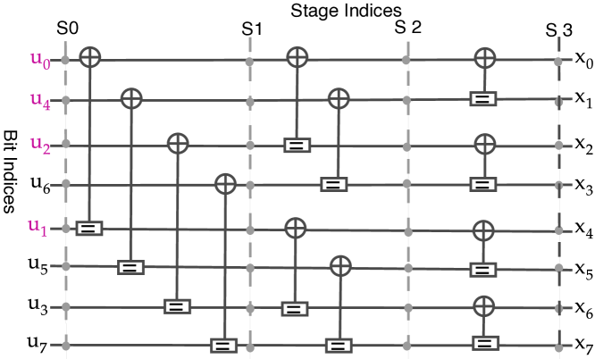
Figure 7: The graph of an $(8,4)$ polar code with bit reversed indexing.

Consequently, the input/output relationship in (31) is established according to the encoder graph representation shown in Figure 7.

$$\begin{array}[]{l l }\begin{aligned} &\mathrm{x}_{0}=\mathrm{u}_{0}\oplus\mathrm{u}_{1}\oplus\mathrm{u}_{2}\oplus\mathrm{u}_{4},\\ &\mathrm{x}_{4}=\mathrm{u}_{1}\oplus\mathrm{u}_{3}\oplus\mathrm{u}_{6},\\ &\mathrm{x}_{2}=\mathrm{u}_{2}\oplus\mathrm{u}_{3}\oplus\mathrm{u}_{6},\\ &\mathrm{x}_{6}=\mathrm{u}_{3}\oplus\mathrm{u}_{7},\end{aligned}&\begin{aligned} &\mathrm{x}_{1}=\mathrm{u}_{4}\oplus\mathrm{u}_{5}\oplus\mathrm{u}_{6},\\ &\mathrm{x}_{5}=\mathrm{u}_{5}\oplus\mathrm{u}_{7},\\ &\mathrm{x}_{3}=\mathrm{u}_{6}\oplus\mathrm{u}_{7},\\ &\mathrm{x}_{7}=\mathrm{u}_{7},\end{aligned}\end{array}$$ (31)

where $\oplus$ denotes addition in $\mathbb{F}_{2}$. The codeword $[\mathrm{x}_{0},\mathrm{x}_{1},\ldots,\mathrm{x}_{7}]$ is transmitted through the physical channels $\mathrm{W}^{8}$, with channel outputs $[\mathrm{y}_{0},\mathrm{y}_{1},\ldots,\mathrm{y}_{7}]$. This structure, comprising coding and channel transmission, creates the channel $\mathrm{W}^{8}:\mathrm{x}_{0},\mathrm{x}_{1},\ldots,\mathrm{x}_{7}\longmapsto\mathrm{y}_{0},\mathrm{y}_{1},\ldots,\mathrm{y}_{7}$.
Initially, polar codes were nonsystematic, but they can be transformed into systematic codes like any linear code. Systematic polar encoding utilizes the standard non-systematic polar encoding apparatus. Systematic polar codes offer improved BER performance compared to non-systematic ones, yet both have identical BLER performance [43]. Systematic polar coding demonstrates greater resilience to error propagation with SC decoder than non-systematic polar coding.

In a linear code, a codeword is a point in the row space of the generator matrix $\mathbf{G}$, so that in $\mathbf{x=zG}$, $\mathbf{z}$ is a codeword, regardless of the particular values in $\mathbf{z}$. One way to do encoding might be to take a message vector $\mathbf{u}$, place it into $\mathrm{K}$ elements of the codeword $\mathbf{x}$, then find a vector $\mathbf{z}$ which fill in the remaining $\mathrm{N}-\mathrm{K}$ elements of $\mathbf{x}$ in such a way that $\mathbf{x}$ is in the row space of $\mathbf{G}$. If $\mathbf{z}$ can be found via linear operations from $\mathbf{u}$ in such a way that the message symbols appear explicitly in $\mathbf{u}$, then systematic encoding has been achieved [7].

$$\mathbf{G}_{\mathsf{8}}=\mathbf{F}^{\otimes 3}=\left[\begin{array}[]{llllllll}1&0&0&0&0&0&0&0\\ 1&1&0&0&0&0&0&0\\ 1&0&1&0&0&0&0&0\\ 1&1&1&1&0&0&0&0\\ 1&0&0&0&1&0&0&0\\ 1&1&0&0&1&1&0&0\\ 1&0&1&0&1&0&1&0\\ 1&1&1&1&1&1&1&1\end{array}\right].$$ (32)

Note that we can perform systematic encoding via the encoder Graph, Arikan’s method, the bit reverse permutation, etc. [7].

III-C 3GPP 5G Polar Codes

In NR, the polar code is used to encode broadcast channel (BCH) as well as downlink control information DCI and uplink control information (UCI). The overall control streams transmission chain from MAC/PHY layer processing schematic is depicted in Figure 8, which describes the transmit-end for the physical uplink/downlink control channel supporting a transport block CRC attachment, code block segmentation and code block CRC attachment, Polar encoding, rate matching code block concatenation. The receiving chain is in line with the transmitting chain in the reverse flow.

(a) Tranmitter end.

(b) Receiver end.

Figure 8: Conceptual illustration of 5G Polar transceiver chain.

3GPP NR uses a variant of the polar code called distributed CRC (D-CRC) polar code, that is, a combination of CRC-assisted and polar codes (PC, which interleaves a CRC-concatenated block and relocates some of the PC bits into the middle positions of this block prior to performing the conventional polar encoding[43]. This allows a decoder to early terminate the decoding process as soon as any parity check is not successful. The D-CRC scheme is important for early termination of decoding process, because the post-CRC interleaver can distribute information and CRC bits such that partial CRC checks can be performed during list decoding and paths failing partial CRC check can be pruned, leading to early termination of decoding. The post-CRC interleaver design is closely tied to the CRC generator polynomial, thus by appropriately selecting the CRC polynomial, one can achieve better early termination gains and maintain acceptable false alarm rate.

1. CRC attachment.
   Assume that the input message (control information) before CRC attachment is $a(0),a(1),\ldots,a(A-1)$, where $A$ is input sequence, parity bits are $p(0),p(2),\ldots,p(L-1)$, $L$ is the number of parity bits. The parity bits are generated by one of the following cyclic generator polynomials.

   A CRC length $L=24$ bits is utilized for the downlink, and depending on the amount of $A$, CRCs of $L=6$ and $L=11$ bits are provided for the uplink.

   For downlink channels, the generator polynomial $\mathrm{g}_{\mathsf{CRC24A}}(\beta)$ is used.

   $$\begin{array}[]{r}\mathrm{g}_{\mathsf{CRC24A}}(\beta)=\left[\beta^{24}+\beta^{23}+\beta^{18}+\beta^{17}+\beta^{14}+\beta^{11}\right.\\ \left.+\beta^{10}+\beta^{7}+\beta^{6}+\beta^{5}+\beta^{4}+\beta^{3}+\beta+1\right].\end{array}$$ (33)

   And for uplink channels, the generator polynomial $\mathrm{g}_{\mathsf{CRC11}}(\beta)$ or $\mathrm{g}_{\mathsf{CRC6}}(\beta)$ is used.

   $$\begin{array}[]{ll}\mathrm{g}_{\mathsf{CRC11}}(\beta)=\left[\beta^{11}+\beta^{10}+\beta^{9}+\beta^{5}+1\right],\\ \mathrm{g}_{\mathsf{CRC6}}(\beta)=\left[\beta^{6}+\beta^{5}+1\right].\end{array}$$ (34)

   The message bits after attaching CRC are $b(1),b(2),\ldots,b(B)$, $B$ is the size of transport block information with CRC bits and $B=A+L$.

   $$b_{k}=\left\{\begin{array}[]{l l}a_{k},&\texttt{ \footnotesize{for} }k=0,1,\ldots,A-1\\ p_{k-A},&\texttt{ \footnotesize{for} }k=A,A+1,\ldots,A+L-1\end{array}\right.$$ (35)

2. Code block segmentation and code block CRC attachment.
   The input bit sequence to the code block segmentation is denoted $a(0),a(1),\ldots,a(A-1)$, where $A$ is no larger than $1706$.

   Assume that the maximum code block size is $A^{\prime}$, assume that $C$ is the total number of code blocks. Thus,

   $$A^{\prime}=\lceil A/C\rceil\cdot C.$$ (36)

   The sequence $c_{r}(0),c_{r}(1),\ldots,c_{r}(A^{\prime}/C-1)$ is used to calculate the CRC parity bits $p_{r}(0),p_{r}(1),\ldots,p_{r}(L-1)$, such that

   $$c_{r,k}=p_{r,\left(k-A^{\prime}/C\right)},\quad A^{\prime}/C\leq k\leq A^{\prime}/C+L-1.$$ (37)

   At the transmitter end, we have the following streamlines:
   The bit sequence input for a given code block to channel coding is denoted by $c(0),c(1),\ldots,c(\mathrm{K}_{r}-1)$ , where $\mathrm{K}_{r}$ is the number of bits in code block number $r$, and each code block is individually encoded. After the encoding process, the resulting coded bit sequence within the $r-th$ code block is denoted by $d_{r}(0),d_{r}(1),\ldots,d_{r}(\mathrm{N}_{r}-1)$ where $\mathrm{N}_{r}=2^{n}$ (code length of the polar code) determined by the following:
   if $E_{r}\leq(9/8)\cdot 2^{\left(\left\lceil\log_{2}E_{r}\right\rceil-1\right)}$ and $\mathrm{K}_{r}/E_{r}<9/16$,
   $\quad n_{1}=\left\lceil\log_{2}E_{r}\right\rceil-1$.
   else $n_{1}=\left\lceil\log_{2}E_{r}\right\rceil$.
   $\mathrm{r}_{\min}=1/8$; $n_{2}=\left\lceil\log_{2}\left(K/\mathrm{r}_{\text{min }}\right)\right\rceil$;
   $n=\max\left\{\min\left\{n_{1},n_{2},n_{\max}\right\},n_{\text{min }}\right\}$,
   where $n_{\min}$ and $n_{\max}$ provide a lower and an upper bound on the code length, respectively. In particular, and $n_{\min}=5$ and $n_{\max}=9$ for the downlink control channel, whereas $n_{\max}=10$ for the uplink control channel. $E_{r}$ is the rate matching output sequence length.
   UE is not expected to be configured with $\mathrm{K}_{r}+n_{PC}>E$ , where $n_{PC}$ is the number of parity check bits.

   • Interleaving.
     The bit sequence $c_{r}(0),c_{r}(1),\ldots,c_{r}(\mathrm{K}_{r}-1)$ is interleaved into bit sequence $c_{r}^{\prime}(0),c_{r}^{\prime}(1),\ldots,c_{r}^{\prime}(\mathrm{K}_{r}-1)$ a follows:

     $$c_{r,k}^{\prime}=c_{r,\Pi(k)},k=0,1,\ldots,\mathrm{K}_{r}-1,r=0,1,\ldots,C-1$$ (38)

     where $\Pi(k)$ is the interleaving pattern [6].

   • Polar encoding.
     The interleaved vector $\mathbf{c}^{\prime}$ is assigned to the information set along with the PC bits, while the remaining bits in the $\mathrm{N}$-bit vector $\mathbf{u}$ are frozen. Hence, $\mathbf{u}=u(0),u(1),\ldots,u(\mathrm{N}-1)$ is generated according to the clause 5.3.1.2 [6]. Denote $\mathbf{G}_{\mathsf{N}_{r}}=\left(\mathbf{G}_{2}\right)^{\otimes n}$ as the $n-th$ Kronecker power of matrix $\mathbf{G}_{2}$ , where $\mathbf{G}_{2}=\left[\begin{array}[]{ll}1&0\\ 1&1\end{array}\right]$, the output after encoding $\mathbf{d}_{r}=d_{r}(0),d_{r}(1),\ldots,d_{r}(\mathrm{N}_{r}-1)$ is obtained by $\mathbf{d}_{r}=\mathbf{u}_{r}\mathbf{G}_{\mathsf{N}_{r}}$, where encoding is performed in $\mathbb{F}_{2}$.

3. Rate matching.
   The rate matching for polar code is defined per coded block and consists of sub-block interleaving, bit collection, and bit interleaving. Sequence of coded bits at the rate matcher input is $d_{r}(0),d_{r}(1),\ldots,d_{r}(\mathrm{N}_{r}-1)$, The output bit sequence from the rate matcher is denoted as $f_{r}(0),f_{r}(1),\ldots,f_{r}(E-1)$. For rate matching, puncturing, shortening ($E_{r}<\mathrm{N}_{R}$), or repetition($E_{r}\geq N_{r}$) are applied to change the $\mathrm{N}_{r}$-bit vector $\bm{s}_{r}$ into the $E_{r}$-bit vector $\bm{e}_{r}$.

   Indeed, the rate matching process encapsulates the following steps:

   • Sub-block interleaving.
     The bits input to the sub-block interleaver are the coded bits $d_{r}(0),d_{r}(1),\ldots,d_{r}(\mathrm{N}_{r}-1)$ . The coded bits $d_{r}(0),d_{r}(1),\ldots,d(\mathrm{N}_{r}-1)$ are divided into 32 sub-blocks. The bits output from the sub-block interleaver are denoted as $s_{r}(0),s_{r}(1),\ldots,s_{r}(\mathrm{N}_{r}-1)$.

   • Bit selection.
     The bit sequence after the sub-block interleaver $s_{r}(0),s_{r}(1),\ldots,s_{r}(\mathrm{N}_{r}-1)$ is written into a circular buffer of length $N$. Denoting by $E_{r}$ the rate matching output sequence length, the bit selection, output bit sequence $e_{r}(0),e_{r}(1),\ldots,e_{r}(\mathrm{E}_{r}-1)$.

   • Interleaving of coded bits.
     The bits sequence $e(0),e(1),\ldots,e(\mathrm{E}_{r}-1)$ is interleaved into bit sequence $f_{r}(0),f_{r}(1),\ldots,f_{r}(E-1)$., where the value of $E_{r}$ is no larger than $8192$.

4. Code block concatenation.
   The code block concatenation consists of sequentially concatenating the rate matching outputs for the different code blocks.

   The input bit sequence for the code block concatenation block are the sequences $f_{r,k}$ , for $r=0,\ldots,C-1$ and $\mathrm{k}=0,\ldots,E_{r}-1$, where $E_{r}$ is the number of rate matched bits for the $r-th$ code block. The output bit sequence from the code block concatenation block is the sequence $g_{\ell}$ for $\ell=0,\ldots,G-1$. Therefore,

   $$g_{\ell}=f_{r,k},\texttt{\footnotesize{where}}\quad 1\leq\ell\leq G,\quad 1\leq k\leq E_{r}.$$ (39)

At the receiver end, the procedure is as follows:

1. Code block de-concatenation.
   Assume that the input message to code block de-concatenation is $y(0),y(1),\ldots,y(G-1)$. The output message from code block de-concatenation is $f_{r,k},\text{where}\quad 1\leq\ell\leq G,\quad 1\leq k\leq E_{r}$.

2. Rate de-matching.
   The purpose of rate de-matching is to convert the code block message to the format that can be used for 5G Polar decoder to process decoding. Rate de-matching is done on each code block independently.

3. Polar decoding.
   The decoding process is done on each code block independently. The subsequent subsection III-D provides more details on polar decoding algorithms.

4. Code block de-segmentation.
   Assume that the output from code block de-segmentation is $\hat{b}(0),\hat{b}(1),\ldots,\hat{b}(B-1)$, where $B$ is the size of original transport block information with attached CRC bits.

5. CRC check.
   CRC check is used to extract the CRC bits in UCI/DCI bits after the information transmitted in 5G NR control channels. Then the extracted CRC bits will be checked with the original CRC bits attached to control information bits before transmitted.

III-D Polar Decoding Algorithms

Two primary polar decoding methods are SC decoder and BP decoder. Unlike SC decoder, BP decoder doesn’t have inter-bit dependence, preventing error propagation and avoiding intermediate hard decisions. It updates LLR values iteratively through right-to-left and left-to-right iterations using LDPC-like update functions. BP decoder supports parallel processing, enhancing throughput for high-speed applications, while SC decoder and its variants have serial decoding characteristics, making parallelization impossible [43] . Moreover, polar decoding can employ various algorithms, including SC decoding and SCL decoding. Polar decoders face challenges in hardware implementation compared to encoders due to complexities: they work with bit probabilities, consider all possible permutations of information blocks, and process each block multiple times for error correction. This leads to higher latency, hardware usage, and power consumption.

1) Successive Cancellation Decoding

The first polar code decoding method, known as successive cancellation (SC), decodes bits one by one, using previous estimations to help determine new ones [7]. SC builds on decoded bits sequentially but suffers from inter-bit dependence and error spread. While it doesn’t perform as well as other decoders alone, it shows promise for list decoding because of its hierarchical structure. Polar codes achieve the Shannon capacity under SC decoding. The computation method for SC is akin to that of LDPC codes, using log-likelihood ratios (LLRs) to estimate bit likelihoods. SC decoding algorithms utilize the log-likelihood function, which can be recursively computed due to the recursive nature of the channel transition function.

Let

$$\lambda_{\mathsf{N}}^{(i)}\left(\mathrm{y}_{0}^{\mathsf{N}-1},\hat{\mathrm{u}}_{0}^{i-1}\right)=\frac{\mathrm{W}_{\mathsf{N}}^{(i)}\left(\mathrm{y}_{0}^{\mathsf{N}-1},\hat{\mathrm{u}}_{0}^{i-1}\mid\mathrm{u}_{i}=0\right)}{\mathrm{W}_{\mathsf{N}}^{(i)}\left(\mathrm{y}_{0}^{\mathsf{N}-1},\hat{\mathrm{u}}_{0}^{i-1}\mid\mathrm{u}_{i}=1\right)},$$ (40)

and let

$$\mathscr{L}_{\mathsf{N}}^{(i)}\left(\mathrm{y}_{0}^{\mathsf{N}-1},\hat{\mathrm{u}}_{0}^{i-1}\right)=\log\lambda_{\mathsf{N}}^{(i)}\left(\mathrm{y}_{0}^{\mathsf{N}-1},\hat{\mathrm{u}}_{0}^{i-1}\right).$$ (41)

This likelihood ratio can be used to estimate the value of the bit $\mathrm{u}_{i}$ using the function $\mathrm{h}_{i}$ defined as

$$\mathrm{h}_{i}\left(\mathrm{y}_{0}^{\mathsf{N}-1},\hat{\mathrm{u}}_{0}^{i-1}\right)=\begin{cases}0&\text{ if }\mathscr{L}_{\mathsf{N}}^{(i)}\left(\mathrm{y}_{0}^{\mathsf{N}-1},\hat{\mathrm{u}}_{0}^{i-1}\right)\geq 0,\\ 1&\text{ otherwise .}\end{cases}$$ (42)

For decoding, if $i\in\mathcal{A}^{c}$ (i.e., the set of frozen bits), then the decoded value is the frozen bit value. Otherwise, it is determined by the $\mathrm{h}$ function:

$$\hat{\mathrm{u}}_{i}=\begin{cases}\mathrm{u}_{i}&i\in\mathcal{A}^{c},\\ \mathrm{h}_{i}\left(\mathrm{y}_{0}^{\mathsf{N}-1},\hat{\mathrm{u}}_{0}^{i-1}\right)&i\in\mathcal{A}\ .\end{cases}$$ (43)

Note that $\hat{\mathrm{u}}^{i}$ depends on the previously estimated values $\hat{\mathrm{u}}_{0}^{i-1}$. This is the essence of SC: bits are estimated in order $\hat{\mathrm{u}}_{0},\hat{\mathrm{u}}_{1},\hat{\mathrm{u}}_{2},\ldots,\hat{\mathrm{u}}_{\mathsf{N}-1}$, with the estimate $\hat{\mathrm{u}}^{i}$ being based upon previously determined bits. Under the polarization idea, since the polarized channels used are assumed to be good, each of the previously determined bits $\hat{\mathrm{u}}_{0}^{i-1}$ are assumed to be good [7].

Moreover the SC decoding principle for polar codes requires only two clarifications: the first is the probability transfer formula on the unit factor graph, and the second is the recursive order. As Figure 9 shows the graph of the unit factor of the polar code, on which there are 8 values, $\mathscr{L}_{1},\mathscr{L}_{2},\mathscr{L}_{3},\mathscr{L}_{4}$ for the LLR values passed to the left and $\mathscr{B}_{1},\mathscr{B}_{2},\mathscr{B}_{3},\mathscr{B}_{4}$ for the hard bit information passed to the right.

The transmission equation is

$$\mathscr{L}_{3}=\mathscr{L}_{1}{\boxplus}\mathscr{L}_{2},$$ (44)

$$\texttt{\small{where}}\ :\ \mathrm{a}\ {\boxplus}\ \mathrm{b}=2\tanh^{-1}\left[\tanh\left(\frac{a}{2}\right)\tanh\left(\frac{b}{2}\right)\right].$$ (45)

$$\mathscr{L}_{4}=\begin{cases}\mathscr{L}_{2}+\mathscr{L}_{1}&\texttt{\small{if }}\mathscr{B}_{3}=0\ .\\ \mathscr{L}_{2}-\mathscr{L}_{1}&\texttt{\small{if }}\mathscr{B}_{3}=1\ .\end{cases}$$ (46)

$$\mathscr{B}_{1}=\mathscr{B}_{3}\oplus\mathscr{B}_{4},$$ (47)

$$\mathscr{B}_{2}=\mathscr{B}_{4}.$$

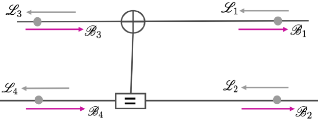
Figure 9: Factor Graph of the SC decoding unit.

In what follows, we’ll describe how the recursive process works using the factor graph shown in Figure 10. First, the decoder needs to find the value called LLR at point 1. To do this, it has to know the LLR values at points 2 and 3. Similarly, to find the LLR at point 2, it needs the LLR values at points 4 and 5, and for point 3, it needs the LLR values at points 6 and 7. However, the LLR values at points 4, 5, 6, and 7 can be figured out directly from the LLR values sent through the channel.

Then, we use equation (44) to calculate the LLR value at point 8 using the LLR value at point 1. Since point 8 is in the bottom left of the unit factor graph, we already know the LLR values of points 2 and 3, so we don’t need to do any more recursion. Once we find the LLR value for point 8, we make a firm decision. After finding the LLR value for the bottom left point, we know the bit decision should move to the right. In other words, we figure out the bit values for points 2 and 3 using equations (45) and (46). Now that points 2 and 3 are in the top left of the unit factor graph, we don’t need to pass hard decision bit values to the right anymore. Next, to find the LLR value at point 9, we first need to calculate the LLR values at points 10 and 11. Since points 10 and 11 are in the bottom left, we can use equation (44) along with the bit decisions of points 2 and 3. We don’t need any more downward recursion. Similarly, we find the LLR value at point 12 using equation (44) and the bit decision of point 9, then we make a decision. As point 12 is in the bottom left, we move the hard decision bit value to the right. At this stage, we compute the binary values of points 10 and 11 using equations (45) and (46), and since they are both in the bottom left, we continue moving binary values to the right for points 4, 5, 6, and 7. Once points 4, 5, 6, and 7 are all in the top left, we stop moving binary values to the right. We repeat this process until the SC decoder has found all LLR values and assigned binary values.

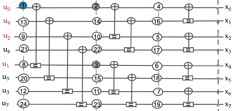
Figure 10: Illustrative instance of a recursive order.

Despite the recursive SC method, the SC method can also be calculated using the node labelling method. To program the LLR recursion process described above and the process of passing the hard decision bit value to the right, the points shown in Figure 10 must be labelled so that they can be programmed in a certain order.

2) Successive Cancellation List Decoding

The SCL decoder was introduced as an extension of the SC decoder. Rather than sequentially computing hard decisions for each bit, it bifurcates into two parallel SC decoders at every decision stage, with each branch maintaining its path metric continuously updated for each path. It’s demonstrated that a list size of 32 is nearly sufficient to reach the ML bound [43].

What is needed is a path metric, computing the likelihood along the entire path of bits. This path metric is established in the following theorem.

Theorem 1.

[73, Theorem 1].
For a path $\ell$ having bits $\hat{\mathrm{u}}_{0}(\ell),\hat{\mathrm{u}}_{1}(\ell),\ldots,\hat{\mathrm{u}}_{i}(\ell)$ and bit number $i\in 0,1,\ldots,\mathrm{N}-1$ , define the path metric as

$$\mathsf{PM}_{\ell}^{(i)}=\sum_{j=0}^{i}\ln\left(1+\exp\left[-\left(1-2\hat{\mathrm{u}}_{j}(\ell)\right)\mathscr{L}_{\mathsf{N}}^{(j)}[\ell]\right]\right)$$ (48)

where

$$\mathscr{L}_{\mathsf{N}}^{(i)}[\ell]=\ln\left(\frac{\mathrm{W}_{\mathsf{N}}^{(i)}\left(y_{0}^{\mathsf{N}-1},\hat{\mathrm{u}}_{0}^{i-1}[\ell]\mid 0\right)}{\mathrm{W}_{\mathsf{N}}^{(i)}\left(\mathrm{y}_{0}^{\mathsf{N}-1},\hat{\mathrm{u}}_{0}^{i-1}[\ell]\mid 1\right)}\right)$$ (49)

is the LLR of the bit $\mathrm{u}_{i}$ given the channel output $\mathrm{y}_{0}^{\mathsf{N}-1}$ and the past trajectory of the path $\hat{u}_{0}^{i-1}[\ell]$. However, the path metric is computed using LLRs, in a numerically stable way[7].

Furthermore, CRC-aided SCL, an extension of the SCL decoder, incorporates a high-rate CRC code appended to the polar code. This addition facilitates the selection of the correct codeword from the final list of paths. It has been observed that in instances where an SCL decoder fails, the correct codeword remains within the list. Hence, the CRC serves as a validation check for each candidate codeword in the list. Polar decoding via BP and SCAN is beyond the scope of this manuscript. Interested readers are encouraged to refer to [59, 79] for BP decoding and [80] for SCAN decoding.

IV Numerical Results

We are interested in the short block regime, i.e. blocks of 20 to 100 bits, we will carry out simulations using a 100-bit block (TB+CRC), with different coding rates from low to high, QPSK modulation coupled with polar and LDPC coding.

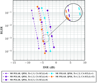
(a) 5G Polar codes.

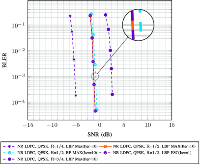
(b) 5G LDPC codes.

Figure 11: Block Error Rate, 100 bits(TBs+CRC), R={1/4, 1/2, 3/4}, NR LDPC (BP, LBP with Early Stop Criteria (ESC), MaxIter=10) and NR POLAR, (CA-SCL, L=1, 8, 32), QPSK modulations, over ($4\times 1$) SIMO, on Non Line-of-Sight (NLOS) TDL channel, 300ns of delay spread.

It can be noticed in Figures 11a that layered belief propagation (LBP) for LDPC decoding often outperforms standard belief propagation (BP) decoding due to its ability to exploit the structure of the LDPC code more efficiently. Concretely, LDPC codes are often constructed with a layered structure, which means that the parity-check matrix can be organized into layers of variable nodes and check nodes. Hence, LBP takes advantage of this structure by decoding the code layer by layer. This can lead to more efficient message passing compared to BP based on "flood" decoding, which updates messages across all variable nodes and check nodes simultaneously. Moreover, LBP typically has lower computational complexity. By decoding the code layer by layer, the complexity of message passing at each iteration can be reduced, since only messages within a layer need to be exchanged. Due to its improved convergence properties and efficient message passing, layered belief propagation decoding tends to provide better error correction performance compared to standard BP decoding. This is particularly advantageous in scenarios with higher levels of noise or more challenging channel conditions. In general, the layered structure and specialized message passing algorithms for layered belief propagation make it a preferred choice for LDPC decoding in many practical applications, offering improved performance, reduced complexity, and better convergence properties. However, the effectiveness of LBP versus BP decoding can be influenced by factors such as the code rate, the operating signal-to-noise ratio (SNR) region, the complexity of the LDPC code structure, and the computational resources available for decoding. For instance, at lower code rate, performance gaps between LBP and standard BP are more pronounced. Conversely, in terms of convergence time, the merits of decoding paired with the early stop criterion (ESC) can be exploited with the LBP decoding which is amenable to a very interesting trade-off between reliability and latency.

Besides, in setups using polar codes, the CRC-aided successive cancellation list (CA-SCL) decoder is highly regarded for its exceptional error correction capabilities compared to the state of art decoders. The performance of the SCL decoder improves with the number of lists ($L$). Increasing $L$ in the SCL decoder enhances BLER performance, as shown in Figures 11b, but leads to higher decoding complexity, requiring more computational resources.

V Conclusions

In conclusion, this paper has served as a comprehensive guide for practitioners and scholars seeking to understand the channel coding and decoding schemes embedded in the 5G NR standard, with a particular focus on LDPC and polar codes. We began by elucidating the design principles underlying these channel codes, providing essential knowledge from both encoding and decoding perspectives. In parallel, we conducted an extensive literature review to establish the current state of research in this field. Notably, we enriched these foundational discussions with detailed, standard-specific insights that are often difficult to extract from technical specification documents. Through this structured approach, we aim to provide a valuable reference for those interested in the complexities of channel coding within the 5G NR framework.

References

- Shannon [1948] C. E. Shannon, “A mathematical theory of communication,” Bell Labs Technical Journal, vol. 27, pp. 379 – 423, 623 – 656, October 1948.
- [2] S. . R. Whitaker, J. Canaris et K. Cameron, ‘’Reed-Solomon VLSI Codec for advanced television," IEEE Trans. Circuits and Systems for video tech, vol. 1, 1991.
- [3] R. Hamming, ‘’Error detecting and error correcting codes," Bell System technical journal, vol. 29, pp. 147-160, 1950.
- [4] A. Hocquenghem, ‘’Codes correcteurs d’erreurs," Chiffres, vol. 2, pp. 147- 156, 1959.
- Gallager [1963] R. G. Gallager, “Low Density Parity Check Codes”, Cambridge, USA: MIT Press, July 1963.
- [6] 3GPP TS 38.212 V16.2.0, “ Technical Specification Group Radio Access Network, Multiplexing and channel coding”, July 2020.
- [7] Todd K. Moon,“Error Correction Coding: Mathematical Methods and Algorithms”, Wiley-Interscience605 Third Avenue New York, NYUnited States, May 2005.
- [8] C. Berrou, A. Glavieux et P. Thitimajshima, ‘’Near shannon limit error correcting coding and decoding :turbo-codes," IEEE International Conference on Communications, vol. 2, May 1993.
- [9] MacKay et Neal, ‘’Near Shannon limit performance of low density parity check codes,” Electronics letters, 1997.
- [10] M. Luby, M. Mitzenmacher, A. Shokrollahi et D. Spielman, ‘’Analysis of low density codes and improved designs using irregular graphs," Proceeding of 30th ACM Symp. on Theory of Computing, 1998.
- Shao et al. [2018] S. Shao et al., "Survey of Turbo, LDPC, and Polar Decoder ASIC Implementations," in IEEE Communications Surveys and Tutorials, vol. 21, no. 3, pp. 2309-2333, thirdquarter 2019.
- Srisupha et al. [2022] T. Srisupha, K. Mueadkhunthod, W. Phakphisut, S. Khittiwitchayakul, K. Puntsri and T. Sopon, "Development of 5G LDPC Experimental Kit," 2022 37th International Technical Conference on Circuits/Systems, Computers and Communications (ITC-CSCC), Phuket, Thailand, 2022, pp. 856-859.
- Belhadj et al. [2021] S. Belhadj and M. L. Abdelmounaim, "On error correction performance of LDPC and Polar codes for the 5G Machine Type Communications," 2021 IEEE International IOT, Electronics and Mechatronics Conference (IEMTRONICS), Toronto, ON, Canada, 2021, pp. 1-4.
- Li et al. [2018] K. -Y. Li, H. -Y. Li, L. Deng, X. -H. Sun, Y. Wang and Z. -P. Shi, "Improved Informed Dynamic Scheduling Strategies for 5G LDPC Codes," 2023 IEEE 23rd International Conference on Communication Technology (ICCT), Wuxi, China, 2023, pp. 74-78.
- Tian and Wang [2022] K. Tian and H. Wang, "A Novel Base Graph Based Static Scheduling Scheme for Layered Decoding of 5G LDPC Codes," in IEEE Communications Letters, vol. 26, no. 7, pp. 1450-1453, July 2022.
- [16] F. Hamidi-Sepehr, A. Nimbalker and G. Ermolaev, "Analysis of 5G LDPC Codes Rate-Matching Design," 2018 IEEE 87th Vehicular Technology Conference (VTC Spring), 2018, pp. 1-5.
- [17] J.H. Bae, A.A. Abotabl, H. Lin, K. Song and J. Lee “An overview of channel coding for 5G NR cellular communications, " APSIPA Transactions on Signal and Information Processing, vol.8, p. e17 2019.
- [18] T. Nguyen, T. N. Tan, and H. Lee, “Efficient QC-LDPC Encoder for 5G New Radio”, Electronics, vol. 8, p. 668, June 2019.
- Liao et al. [2018] S. Liao, Y. Zhan, Z. Shi and L. Yang, "A High Throughput and Flexible Rate 5G NR LDPC Encoder on a Single GPU," 2021 23rd International Conference on Advanced Communication Technology (ICACT), PyeongChang, Korea (South), 2021, pp. 29-34.
- Tarver et al. [2021] C. Tarver, M. Tonnemacher, H. Chen, J. Zhang and J. R. Cavallaro, "GPU-Based, LDPC Decoding for 5G and Beyond," in IEEE Open Journal of Circuits and Systems, vol. 2, pp. 278-290, 2021.
- Nadal and Baghdadi [2021] J. Nadal and A. Baghdadi, "Parallel and Flexible 5G LDPC Decoder Architecture Targeting FPGA," in IEEE Transactions on Very Large Scale Integration (VLSI) Systems, vol. 29, no. 6, pp. 1141-1151, June 2021.
- Xu et al. [2021] Y. Xu, W. Wang, Z. Xu and X. Gao, "AVX-512 Based Software Decoding for 5G LDPC Codes," 2019 IEEE International Workshop on Signal Processing Systems (SiPS), Nanjing, China, 2019, pp. 54-59.
- Sy [2023] Mody Sy, "Optimization Strategies for Low Latency 5G NR LDPC Decoding on General Purpose Processor", 5-th IEEE International Conference on Control, Communication and Computing (ICCC 2023),Thiruvananthapuram, India, May 19-20, 2023.
- Li et al. [2021] 2. M. Li, V. Derudder, K. Bertrand, C. Desset and A. Bourdoux, "High-Speed LDPC Decoders Towards 1 Tb/s," in IEEE Transactions on Circuits and Systems I: Regular Papers, vol. 68, no. 5, pp. 2224-2233, May 2021.
- Aronov et al. [2019] A. Aronov, L. Kazakevich, J. Mack, F. Schreider and S. Newton, "5G NR LDPC Decoding Performance Comparison between GPU and FPGA Platforms," 2019 IEEE Long Island Systems, Applications and Technology Conference (LISAT), Farmingdale, NY, USA, 2019, pp. 1-6.
- Rao and Babu. [2019] K. D. Rao and T. A. Babu, "Performance Analysis of QC-LDPC and Polar Codes for eMBB in 5G Systems," 2019 International Conference on Electrical, Electronics and Computer Engineering (UPCON), Aligarh, India, 2019, pp. 1-6.
- Wu et al. [2019] H. Wu and H. Wang, "A High Throughput Implementation of QC-LDPC Codes for 5G NR," in IEEE Access, vol. 7, pp. 185373-185384, 2019.
- Ivanov et al. [2023] F. Ivanov and A. Kuvshinov, "On the Serial Concatenation of LDPC Codes," 2023 16th International Conference on Advanced Technologies, Systems and Services in Telecommunications (TELSIKS), Nis, Serbia, 2023, pp. 228-231.
- Song et al. [2023] L. Song, S. Yu and Q. Huang, "Low-density parity-check codes: Highway to channel capacity," in China Communications, vol. 20, no. 2, pp. 235-256, Feb. 2023.
- Ahn et al. [2019] S. -K. Ahn, K. -J. Kim, S. Myung, S. -I. Park and K. Yang, "Comparison of Low-Density Parity-Check Codes in ATSC 3.0 and 5G Standards," in IEEE Transactions on Broadcasting, vol. 65, no. 3, pp. 489-495, Sept. 2019.
- Cui et al. [2021] H. Cui, F. Ghaffari, K. Le, D. Declercq, J. Lin and Z. Wang, "Design of High-Performance and Area-Efficient Decoder for 5G LDPC Codes," in IEEE Transactions on Circuits and Systems I: Regular Papers, vol. 68, no. 2, pp. 879-891, Feb. 2021.
- Trung et al. [2019] K. Le Trung, F. Ghaffari and D. Declercq, "An Adaptation of Min-Sum Decoder for 5G Low-Density Parity-Check Codes," 2019 IEEE International Symposium on Circuits and Systems (ISCAS), Sapporo, Japan, 2019.
- Jayawickrama and He [2022] B. A. Jayawickrama and Y. He, "Improved Layered Normalized Min-Sum Algorithm for 5G NR LDPC," in IEEE Wireless Communications Letters, vol. 11, no. 9, pp. 2015-2018, Sept. 2022.
- Li et al. [2020] L. Li, J. Xu, J. Xu and L. Hu, "LDPC design for 5G NR URLLC and mMTC," 2020 International Wireless Communications and Mobile Computing (IWCMC), Limassol, Cyprus, 2020, pp. 1071-1076.
- Wu and Wang [2019] H. Wu and H. Wang, "Decoding Latency of LDPC Codes in 5G NR," 2019 29th International Telecommunication Networks and Applications Conference (ITNAC), Auckland, New Zealand, 2019, pp. 1-5.
- Sun and Jiang. [2018] K. Sun and M. Jiang, "A Hybrid Decoding Algorithm for Low-Rate LDPC codes in 5G," 2018 10th International Conference on Wireless Communications and Signal Processing (WCSP), 2018, pp. 1-5.
- Dai et al. [2021] J. Dai et al., "Learning to Decode Protograph LDPC Codes," in IEEE Journal on Selected Areas in Communications, vol. 39, no. 7, pp. 1983-1999, July 2021.
- Shah and Vasavada [2021] N. Shah and Y. Vasavada, "Neural Layered Decoding of 5G LDPC Codes," in IEEE Communications Letters, vol. 25, no. 11, pp. 3590-3593, Nov. 2021.
- Tang et al. [2021] Y. Tang, L. Zhou, S. Zhang, C. Chen and L. Wang, "Normalized Neural Network for Belief Propagation LDPC Decoding," 2021 IEEE International Conference on Networking, Sensing and Control (ICNSC), Xiamen, China, 2021, pp. 1-5.
- Andreev et al. [2021] K. Andreev, A. Frolov, G. Svistunov, K. Wu and J. Liang, "Deep Neural Network Based Decoding of Short 5G LDPC Codes," 2021 XVII International Symposium "Problems of Redundancy in Information and Control Systems" (REDUNDANCY), Moscow, Russian Federation, 2021, pp. 155-160
- [41] H. Xiao-Yu, M. Fossorier et E. ELEFTHERIOU, ‘’On the computation of the minimum distance of low-density parity-check codes," IEEE International Conference on Communications, 2004.
- [42] L. Zhang, Q. Huang, S. Lin, K. Abdel-Ghaffar et I. F. Blake, ‘’Quasi-cyclic LDPC codes: an algebraic construction rank analysis and codes on latin squares," IEEE Trans. Commun., vol. 58, pp. 3126-3139, Nov 2010.
- [43] S. Ahmadi, “ 5G NR, Architecture, Technology, Implementation, and Operation of 3GPP New Radio Standard”,London, United Kingdom : Academic Press, an imprint of Elsevier, 2019.
- [44] LIFANG WANG “Implementation of Low-Density Parity-Check codes for 5G NR shared channels,” master Thesis, August 30, 2021.
- [45] Jinghu Chen, R. M. Tanner, C. Jones and Yan Li, "Improved min-sum decoding algorithms for irregular LDPC codes," Proceedings. International Symposium on Information Theory, 2005. ISIT 2005., Adelaide, SA, Australia, 2005, pp. 449-453,
- [46] D. E. Hocevar, "A reduced complexity decoder architecture via layered decoding of LDPC codes," IEEE Workshop onSignal Processing Systems, 2004. SIPS 2004., Austin, TX, USA, 2004, pp. 107-112.
- [47] J. Zhang, Y. Lei, and Y. Jin, "Check-node lazy scheduling approach for layered belief propagation decoding algorithm," Electron. Lett., vol. 50, no. 4, pp. 278–279, Feb. 2014.
- Arikan [2029] E. Arikan, “Channel Polarization: A Method for constructing Capacity-Achieving Codes for Symmetric Binary-Input Memoryless Channels”, IEEE Transactions on Information Theory, vol. 55, No. 7, pp. 3051-3073, July 2009.
- [49] A. Elkelesh, M. Ebada, “Polar Codes", Institut fur Nachrichtenubertragung. WebDemos.
- Bioglio et al. [2021] V. Bioglio, C. Condo and I. Land, "Design of Polar Codes in 5G New Radio," in IEEE Communications Surveys and Tutorials, vol. 23, no. 1, pp. 29-40, Firstquarter 2021.
- Gamage et al. [2020] H. Gamage, V. Ranasinghe, N. Rajatheva and M. Latva-aho, "Low Latency Decoder for Short Blocklength Polar Codes," 2020 European Conference on Networks and Communications (EuCNC), Dubrovnik, Croatia, 2020, pp. 305-310.
- Geiselhart et al. [2020] M. Geiselhart, A. Elkelesh, M. Ebada, S. Cammerer and S. ten Brink, "CRC-Aided Belief Propagation List Decoding of Polar Codes," 2020 IEEE International Symposium on Information Theory (ISIT), Los Angeles, CA, USA, 2020, pp. 395-400, doi: 10.1109/ISIT44484.2020.9174249.
- Piao et al. [2019] J. Piao, J. Dai and K. Niu, "CRC-Aided Sphere Decoding for Short Polar Codes," in IEEE Communications Letters, vol. 23, no. 2, pp. 210-213, Feb. 2019.
- Cavatassi et al. [2019] A. Cavatassi, T. Tonnellier and W. J. Gross, "Asymmetric Construction of Low-Latency and Length-Flexible Polar Codes," ICC 2019 - 2019 IEEE International Conference on Communications (ICC), Shanghai, China, 2019, pp. 1-6.
- Shen et al. [2022] Y. Shen, W. Zhou, Y. Huang, Z. Zhang, X. You and C. Zhang, "Fast Iterative Soft-Output List Decoding of Polar Codes," in IEEE Transactions on Signal Processing, vol. 70, pp. 1361-1376, 2022.
- Kaykac et al. [2020] Z. B. Kaykac Egilmez, L. Xiang, R. G. Maunder and L. Hanzo, "The Development, Operation and Performance of the 5G Polar Codes," in IEEE Communications Surveys and Tutorials, vol. 22, no. 1, pp. 96-122, Firstquarter 2020.
- Ercan et al. [2020] F. Ercan, T. Tonnellier, N. Doan and W. J. Gross, "Practical Dynamic SC-Flip Polar Decoders: Algorithm and Implementation," in IEEE Transactions on Signal Processing, vol. 68, pp. 5441-5456, 2020.
- Kestel et al. [2020] C. Kestel et al., "A 506Gbit/s Polar Successive Cancellation List Decoder with CRC," 2020 IEEE 31st Annual International Symposium on Personal, Indoor and Mobile Radio Communications, London, UK, 2020.
- Arli and Gazi [2021] A. Ç. Arli and O. Gazi, "A survey on belief propagation decoding of polar codes," in China Communications, vol. 18, no. 8, pp. 133-168, Aug. 2021.
- Sun et al. [2019] C. Sun, Z. Fei, C. Cao, X. Wang and D. Jia, "Low Complexity Polar Decoder for 5G Embb Control Channel," in IEEE Access, vol. 7, pp. 50710-50717, 2019.
- Sarkis et al. [2014a] G. Sarkis, P. Giard, C. Thibeault and W. J. Gross, "Autogenerating software polar decoders," 2014 IEEE Global Conference on Signal and Information Processing (GlobalSIP), Atlanta, GA, USA, 2014, pp. 6-10.
- Sarkis et al. [2014b] G. Sarkis, P. Giard, A. Vardy, C. Thibeault and W. J. Gross, "Increasing the speed of polar list decoders," 2014 IEEE Workshop on Signal Processing Systems (SiPS), Belfast, UK, 2014, pp. 1-6.
- Kam et al. [2021] D. Kam, H. Yoo and Y. Lee, "Ultralow-Latency Successive Cancellation Polar Decoding Architecture Using Tree-Level Parallelism," in IEEE Transactions on Very Large Scale Integration (VLSI) Systems, vol. 29, no. 6, pp. 1083-1094, June 2021.
- Xiang et al. [2020] L. Xiang, S. Zhong, R. G. Maunder and L. Hanzo, "Reduced-Complexity Low-Latency Logarithmic Successive Cancellation Stack Polar Decoding for 5G New Radio and Its Software Implementation," in IEEE Transactions on Vehicular Technology, vol. 69, no. 11, pp. 12449-12458, Nov. 2020.
- Rezaei et al. [2022] H. Rezaei, V. Ranasinghe, N. Rajatheva, M. Latva-aho, G. Park and O. -S. Park, "Implementation of Ultra-Fast Polar Decoders," 2022 IEEE International Conference on Communications Workshops (ICC Workshops), Seoul, Korea, Republic of, 2022, pp. 235-241.
- Liu et al. [2022] Z. Liu, R. Liu and H. Zhang, "High-Throughput Adaptive List Decoding Architecture for Polar Codes on GPU," in IEEE Transactions on Signal Processing, vol. 70, pp. 878-889, 2022.
- Doan et al. [2019a] N. Doan, S. A. Hashemi, E. N. Mambou, T. Tonnellier and W. J. Gross, "Neural Belief Propagation Decoding of CRC-Polar Concatenated Codes," ICC 2019 - 2019 IEEE International Conference on Communications (ICC), Shanghai, China, 2019, pp. 1-6.
- Hashemi et al. [2019] S. A. Hashemi, N. Doan, T. Tonnellier and W. J. Gross, "Deep-Learning-Aided Successive-Cancellation Decoding of Polar Codes," 2019 53rd Asilomar Conference on Signals, Systems, and Computers, Pacific Grove, CA, USA, 2019, pp. 532-536.
- Doan et al. [2020] N. Doan, S. A. Hashemi and W. J. Gross, "Decoding Polar Codes with Reinforcement Learning," GLOBECOM 2020 - 2020 IEEE Global Communications Conference, Taipei, Taiwan, 2020.
- Doan et al. [2021] N. Doan, S. A. Hashemi, F. Ercan and W. J. Gross, "Fast SC-Flip Decoding of Polar Codes with Reinforcement Learning," ICC 2021 - IEEE International Conference on Communications, Montreal, QC, Canada, 2021, pp. 1-6.
- Wodiany and Pop [2019] I. Wodiany and A. Pop, "Low-Precision Neural Network Decoding of Polar Codes," 2019 IEEE 20th International Workshop on Signal Processing Advances in Wireless Communications (SPAWC), Cannes, France, 2019.
- Wen et al. [2019] C. Wen, J. Xiong, L. Gui and L. Zhang, "A BP-NN Decoding Algorithm for Polar Codes," 2019 11th International Conference on Wireless Communications and Signal Processing (WCSP), Xi’an, China, 2019.
- Stimming et al. [2015] A. Balatsoukas-Stimming, M. B. Parizi and A. Burg, "LLR-Based Successive Cancellation List Decoding of Polar Codes," in IEEE Transactions on Signal Processing, vol. 63, no. 19, pp. 5165-5179, Oct.1, 2015.
- Tal and Vardy. [2015] I. Tal and A. Vardy, "List Decoding of Polar Codes," in IEEE Transactions on Information Theory, vol. 61, no. 5, pp. 2213-2226, May 2015.
- Zhang et al. [2017] Q. Zhang, A. Liu, X. Pan and K. Pan, "CRC Code Design for List Decoding of Polar Codes," in IEEE Communications Letters, vol. 21, no. 6, pp. 1229-1232, June 2017.
- Arikan [2008] E. Arikan, "Channel polarization: A method for constructing capacity-achieving codes," 2008 IEEE International Symposium on Information Theory, Toronto, ON, Canada, 2008, pp. 1173-1177.
- Fayyaz [2013] U. U. Fayyaz and J. R. Barry, "Polar codes for partial response channels," 2013 IEEE International Conference on Communications (ICC), Budapest, Hungary, 2013, pp. 4337-4341.
- [78] B. Yuan and K. K. Parhi, "Early Stopping Criteria for Energy-Efficient Low-Latency Belief-Propagation Polar Code Decoders," in IEEE Transactions on Signal Processing, vol. 62, no. 24, pp. 6496-6506, Dec.15, 2014.
- Wang et al. [2019] Y. Wang, S. Zhang, C. Zhang, X. Chen and S. Xu, "A Low-Complexity Belief Propagation Based Decoding Scheme for Polar Codes - Decodability Detection and Early Stopping Prediction," in IEEE Access, vol. 7, pp. 159808-159820, 2019.
- Fayyaz [2014] U. U. Fayyaz and J. R. Barry, "Low-Complexity Soft-Output Decoding of Polar Codes," in IEEE Journal on Selected Areas in Communications, vol. 32, no. 5, pp. 958-966, May 2014