Exploring the stellar streams and satellites around the giant low surface brightness galaxy Malin 1

Context. Giant Low Surface Brightness galaxies (gLSBGs), such as Malin 1, host extended stellar and gaseous disks exceeding 100 kpc in radius. Their formation and evolution remain debated, with interactions with satellite galaxies and accretion streams proposed as key contributors. Malin 1 has multiple satellites, including Malin 1A, Malin 1B, and the newly reported Malin 1C, along with SDSS J123708.91+142253.2 (eM1) at 350 kpc. Additionally, it exhibits two giant stellar streams, the largest extending 200 kpc in projection, likely linked to past interactions.

Aims. We investigate the orbital dynamics of Malin 1’s satellites and their relationship with the observed stellar streams, testing their consistency with different formation scenarios.

Methods. We constructed gravitational potentials using optical and H I rotation curve data, incorporating stellar, gaseous, and dark matter components. We explored a wide parameter space to determine whether the candidate progenitors of the stellar streams could have originated from past interactions, testing both Navarro-Frenk-White (NFW) and isothermal halo profiles.

Results. Among ten explored scenarios, seven produced bound orbital solutions. The isothermal halo model, with $M_{\rm Virial}\approx 3.8\times 10^{12}\,M_{\odot}$ and $R_{\rm Virial}\approx 323$ kpc, favors bound satellite orbits more than the NFW model ($1.7\times 10^{12}\,M_{\odot}$). We find that eM1 probably had a pericenter passage 1.3 Gyr ago, Malin 1A around 1.4 Gyr ago, and Malin 1B’s leading arm may be experiencing one now. Malin 1C displays both leading and trailing arms. Furthermore, we identify three unbound orbital solutions that could link eM1, Malin 1A, or Malin 1B to the streams.

Conclusions. The alignment of satellites and streams supports the idea that past interactions contributed to Malin 1’s morphology, enriched its gas reservoir, and influenced the development of its extended disk, providing insights into the evolution of gLSBGs.

1 Introduction

Disney (1976) suggested the possibility that there are galaxies with a Surface Brightness (SB) lower than the empirical limit proposed by Freeman (1970), which defined the characteristic central surface brightness of disk galaxies around $21.65$ $B$ mag arcsec^-2. This threshold was based on observations of High-Surface Brightness spirals and was initially thought to represent a universal feature of disk galaxies. Since then, the discovery rate of Low-Surface-Brightness Galaxies (LSBGs) has been boosted by advances in observational techniques and deeper sky surveys, leading to a growing recognition of their importance in galactic formation and evolution (Du et al., 2020).

In general terms, LSBGs exhibit a central surface brightness fainter than $23.5$ $B$ mag arcsec^-2 (Impey & Bothun, 1997). These galaxies display poor star formation rates, low metallicity, and extended HI gas discs; characteristics shared with giant-LSBGs (gLSBGs), which appear as massive systems typically existing in isolation and having sizes larger than the size of the Milky Way (MW), to the 25th isophote (Das, 2013).

Malin 1, one of the most iconic gLSBGs due to its immense size and faintness, was discovered serendipitously by Bothun et al. (1987). This particular gLSBG has a bar structure and shows a LINER nucleus (Barth, 2007). The evidence indicates that the bar resulted from several star formation events along with the discovery of compact sources, pointing to a possible double nucleus system (Johnston et al., 2024). At its core ($<$$10$ kpc), there is an ordinary High Surface Brightness Galaxy (HSBG), while the periphery displays a LSB disk (Barth, 2007). The final component features the most extensive known stellar disc and features with extraordinary detail, collecting data many hours in the $r$ and $g$ band, reaching a surface brightness of approximately 28.0 $B$ mag arcsec^-2 (Galaz et al., 2015; Boissier et al., 2016), and possesses an optical diameter near 240 kpc (Moore & Parker, 2006). Ogle et al. (2016, 2019) report the discovery of a large sample of the most optically luminous, biggest, and massive spiral galaxies in the universe, called super spirals, which could be analogous to Malin 1; however, Malin 1 is still the largest stellar disk known (Ogle et al., 2016, 2019) but with a much lower star formation rate $\sim 1.2M_{\odot}yr^{-1}$ (Lelli et al., 2010; Junais et al., 2024). The galaxy also possesses a large HI gas reservoir with a mass $4-7\times 10^{10}M_{\odot}$ (Pickering et al., 1997; Lelli et al., 2010). It also has a high specific angular momentum (Di Teodoro et al., 2023; Boissier et al., 2016; Salinas & Galaz, 2021), and an extended flat rotation curve (Lelli et al., 2010; Pickering et al., 1997), all of which suggest the presence of a vast dark mater halo (Mo, 2010).

Malin 1 also presents HII regions, a radial decrease in the star formation rate’s surface density, reduced metal content, and flattening in the outer disk (Junais et al., 2024). These characteristics provide clues about the development of the disc, with the most likely scenario involving the accretion of a preenriched gas from a previous merger (Junais et al., 2024; Zhu et al., 2018). Furthermore, the galaxy is characterised by a low dust content and a minimal presence of molecular gas (Gerritsen & De Blok, 1999; Galaz et al., 2022; Junais et al., 2024; Galaz et al., 2024).

Moreover, an optical map reveals a cavity in the southern part between the arms (Galaz et al., 2015). This cavity could be due to feedback from star formation, as the HI map shows a nearby asymmetric substructure (Lelli et al., 2010), or the action of supernova-driven winds expelling gas, similar to phenomena observed in other galaxies such as the Hoag galaxy (Bannikova, 2018), the Fireworks galaxy (Blair et al., 2019), NGC 1300 (Maeda et al., 2022), or the gLSBG UGC1382 (Saburova & Cherepashchuk, 2021). A northern warp in the HI disk shows nonaxisymmetry, possible due to the accretion of a paired system of two gas-rich satellite galaxies. This can be evidence of ongoing interaction (Saha et al., 2021).

Studies reveal that Malin 1 interacts with at least two companion galaxies, identified as Malin 1B and exo-Malin 1 (Reshetnikov et al., 2010; Galaz et al., 2015). In addition, Malin 1A is part of the Malin 1 system and, together with Malin 1B, they are classified as compact ellipticals (cE) (Saburova & Cherepashchuk, 2021). A recent study by Junais et al. (2024) identified several $H\alpha$ regions, including Malin 1C, which is part of the Malin 1 galaxy and possibly an ultra-diffuse galaxy (UDG) interacting with the core galaxy (Ji et al., 2021). Malin 1C has possibly been stripped of gas and outlying stars by tidal interactions (Kazantzidis S. et al., 2003).

Malin 1B and exo-Malin 1 are situated at distances of $14$ kpc and $350$ kpc, toward the southeast and northwest, respectively (Reshetnikov et al., 2010). According to Saha et al. (2021), exo-Malin 1 may play a role in star formation within the central bar, while the accretion of Malin 1B could bolster star formation in the arms and bulge (Saha et al., 2021). As noted by Saburova et al. (2023) and Peñarrubia et al. (2006), extended discs in giant low surface brightness might develop through minor mergers involving gas-rich satellites, possibly applicable to exo-Malin 1, Malin 1B, Malin 1A, and Malin 1C.

Tidal stellar streams exemplify the continuous merging and accretion of galaxies, a key process in the formation of structure within the Universe (Niederste-Ostholt et al., 2012).

A large stellar stream located at the edge of the Coma galaxy cluster, beyond the Local Group, provides crucial insights into the gravitational potential of its surroundings (Román et al., 2023). Studying the brightness properties of the stream progenitors, it appears that they were accreted in relatively early epochs Vera-Casanova et al. (2022).

As Román et al. (2023) pointed out, such giant, faint stellar streams may exist in galaxy clusters and groups according to $\Lambda$-CDM. So, the presence of streams in the Malin 1 system could be the evidence that not all gLSBGs are isolated, in contrast to Das (2013), who argued that these giants are usually found isolated, often near the edges of voids, and that their lack of interactions contributes to their slow evolution.

Regarding other satellites and tidal streams, several well-studied examples highlight the remnants of disrupted dwarf galaxies. One such case is the Sagittarius tidal stream, which originates from the Sagittarius dwarf galaxy. Interestingly, some stream progenitors are unexpectedly distant from their associated tidal debris (Niederste-Ostholt et al., 2012), often separated by several to tens of degrees (Bonaca et al., 2021).

Another striking example is the extensive stellar stream discovered in the Coma cluster. This structure extends over 500 kpc in length and is also believed to have formed from the disruption of a dwarf galaxy (Román et al., 2023).

Furthermore, the position of a satellite along its orbit can determine whether it appears closer to, farther from, or in between its own tidal debris or stream components. As shown in studies of the Sagittarius stream, tidal tails do not always remain symmetrically distributed around their progenitor. Instead, their structure evolves due to orbital dynamics, where the leading and trailing arms undergo compression or stretching depending on their location along the orbit (Niederste-Ostholt et al., 2012). At the apocenter, the debris tends to pile up, forming overdensities, while at the pericenter, the tidal arms stretch out as the material moves faster along the orbit.

Within Malin 1, possible streams labelled A and B have been found, possibly indicating historical interactions (Galaz et al., 2015). Stream B is significantly extended, reaching up to $200$ kpc from the centre of Malin 1, and may serve as evidence of a historical interaction between exo-Malin 1 and Malin 1 (Reshetnikov et al., 2010; Galaz et al., 2015). The relationship between the two streams remains unclear, as does the status of their progenitor galaxy: whether it is still intact or has been dismantled. Understanding the origins of these streams is crucial for deciphering the dynamics of the Malin 1 system. In particular, stream B contacts at least two arms of Malin 1, a detail clearly illustrated at the beginning of stream B that begins in the centre of Malin 1 within label 3 in Fig. 1.

The possibility that stream A is concurrently connected with Malin 1B (Reshetnikov et al., 2010) and/or Malin 1A (Saburova & Cherepashchuk, 2021) supports the hypothesis of a past merger. Malin 1A and Malin 1B, both compact ellipticals (cE), could have experienced tidal stripping, potentially explaining their compact nature. If further stripping occurs, they might evolve into objects similar to Ultra-Compact Dwarfs (UCDs), as suggested by Bekki et al. (2001). Meanwhile, Malin 1C’s classification remains unclear: it could be either an ultra-diffuse Galaxy (UDG) (Ji et al., 2021) or a young star-forming region (Junais et al., 2024), possibly linked to past interactions.

Current orbital configurations significantly influence tidal stream arrangements, impacting both the leading and trailing arms, and possibly affecting the remnant bound core. This effect is substantiated by various simulation studies (see Fig. 1 in Niederste-Ostholt et al., 2012). Consequently, Malin 1C and Malin 1A could play such roles. Alternatively, Malin 1B might be involved if streams A and B are connected.

Various hypotheses concerning the origin of gLSBG are detailed here. According to Noguchi (2001), gLSBGs evolve from standard spiral galaxies through dynamic changes over time. Their formation is influenced by environmental factors, including large galaxies in voids that feature conventional bulges coupled with extensive LSB disks (Hoffman et al., 1992). Within the hierarchical formation paradigm, mergers between a central galaxy and its satellite companions may explain the considerable size observed (Peñarrubia et al., 2006). Although the origins and properties remain partially unknown, some cosmological simulations point to these alignment-driven mergers as the key to such large-scale development (Zhu et al., 2023). Moreover, Zhu et al. (2018) identified that a notable share of the cold gas at redshift zero emerged from cooling of a hot halo gas, a process initiated following the merger of two deeply interwoven galaxies.

The $\Lambda$-Cold Dark Matter ($\Lambda$CDM) cosmology theory suggests that the disintegration of satellite galaxies is a continuous process in the lifetime of massive galaxies (Martínez-Delgado et al., 2023; Miro-Carretero et al., 2024). The expansive size of the disk might result from the impact of two or more galaxies merging. This formation mechanism aligns with existing theories of galaxy formation (Zhu et al., 2018).

Research involving cosmological simulations (Zhu et al., 2018; Nelson et al., 2018; Pillepich et al., 2018) illustrates that smaller galaxies, often termed intruders, can interact with larger galaxies, leading to the formation of a giant Low-Surface Brightness galaxy (gLSBG) that shares notable similarities with Malin 1. Likewise, Mapelli et al. (2007) proposed that stimulated accretion might explain the exceptionally large disk size of Malin 1. Additionally, Zhu et al. (2018) indicated that a collision involving three galaxies could produce a gas-rich giant low-surface brightness galaxy.

This paper investigates Malin 1 and its surroundings. We analyse the orbital configurations of its satellite galaxies, including both leading and trailing segments, to comprehend their impact on its structure, kinematics, and evolutionary progression.

The structure of this article is as follows. Section 2 describes the observed substructures. Section 3 details the modelling approach for the Malin 1 system. Section 3.1 provides observational data and associated constraints. Section 3.2 discusses the gravitational potential of Malin 1, and Section 3.3 outlines scenarios to explore progenitor candidates of the stellar streams, including initial setups. Section 4 evaluates the results, and Section 5 discusses the physical implications of the findings. The conclusion is found in Section 6. Furthermore, two appendices summarise the optimal parameters and describe how prior knowledge is integrated into our model.

For our calculations, we used a flat $\Lambda$CDM cosmology with H₀ set at 70 km s^-1 Mpc^-1, $\Omega_{\rm M}=0.27$, and $\Omega_{\Lambda}=0.73$. This results in a projected angular scale of 1.557 kpc arcsec^-1 and a luminosity distance of 377 Mpc.

2 Observed substructures in the Malin 1 system

This section offers a summary of the features identified in the optical image of Malin 1 (Galaz et al., 2015). The environment of Malin 1, observed in the $g$ and $r$ bands with the $6.5$ m Magellan/Clay telescope, is shown in Fig. 1, and the listed substructures are indicated by arrows that follow the same numbering. The essential characteristics are listed in Table 1. Among the standout features of Malin 1, the following are noteworthy:

Figure 1: Optical view in $g$, and $r$ band, of Malin 1 and their environment using Magellan/Clay telescope Galaz et al. (2015). In the figure we convert the original equatorial coordinates, using the projected angular scale of $1.557$ kpc (Galaz et al., 2015), to $X$, $Y$ in [kpc] units centred on the core of Malin 1. In the larger sub-panel (4), the color scale deploys arbitrary intensity units, and these units are consistent throughout all sub-panels. Labels include: 1. Optical view, $g$, and $r$ band, of Malin 1 Galaz et al. (2015). 2. Proposed stream A, possible linking Malin 1A, Malin 1B, and Malin 1. 3. Proposed stream B, presumably connecting Malin 1 to exo-Malin 1, and possibly Malin 1C (see point 10. in this caption). 4. The satellite galaxy SDSS J123708.91+142253.2 (Reshetnikov et al., 2010), referred to as exo-Malin 1, located at coordinates $X=-211.38$ kpc, $277.78$ kpc. The approximate separation between exo-Malin 1 and Malin 1 is $\sim 350\;$ kpc (Reshetnikov et al., 2010; Galaz et al., 2015). In their zoom-in image, there is a clear offset of the central SB peak from the geometrical centre, which could be result of external perturbations. 5. Malin 1B, a compact elliptical (cE) interacting galaxy (Saburova & Cherepashchuk, 2021), accompanied by its amplified image. 6. Malin 1A, another cE interacting galaxy also examined by Saburova & Cherepashchuk (2021), along with its amplified image. 7. A proposed cavity highlighted with a red ellipse, which might be an area of decreased gas density. 8. A more distant galaxy in the backdrop ($z$=0.3639). 9. Yellow ellipse indicating clumps within the spiral arms; their structure suggests regions of star formation or clusters of newly formed stars, based on VLT-MUSE observations (Junais et al., 2024). 10. Considered a possible Ultra Diffuse Galaxy (UDG) (Ji et al., 2021), VLT-MUSE (Junais et al., 2024) identified this as a young star formation region with redshift $z=0.08292$. It is situated at $\sim 46.75$ kpc from Malin 1 centre, forming part of the Malin 1 environment, and is referred to here as Malin 1C. An amplified image of Malin 1C is also available in colour to the left of Malin 1C.

Table 1: Properties of the Malin 1 galaxy. Morphology, luminosity distance $D_{L}$, absolute V-band magnitude, $M_{V}$, central surface brightness in the B and V band, $\mu_{0,B}$, $\mu_{0,V}$, respectively, HI gas mass range, $M_{HI}$, active galactic nucleus (AGN), right ascension, $\alpha$, declination, $\delta$, redshift, $z$, galaxy’s Heliocentric systemic velocity, $V_{\odot}^{\star}$, optical diameter, $D_{opt}$, inclination, $i$, Luminosity r-band, $L_{r}$

Property
Morphology	SB0/a a
$D_{L}$	$\sim 377\pm 8$ Mpc b
${\rm M_{V}}$	$-22.9\pm 0.4$ mag c
$\mu_{0,B}$	$\sim 28.0\;\text{mag}\;\text{arcsec}^{-2}$ d
$\mu_{0,V}$	$\sim 25.5\;\text{mag}\;\text{arcsec}^{-2}$ e
$M_{\mathrm{HI}}$	$4-7\times 10^{10}\mathrm{M_{\odot}}$ f
AGN	LINER g
$\alpha$ $(J2000)$	$12^{h}36^{m}59.35^{s}$ h
$\delta$ $(J2000)$	$+14^{\circ}19^{\prime}49.16^{\prime\prime}$ h
$z$	$0.0827002$ h
${V_{\odot}^{\star}}$	$\mathrm{24775}\pm 10\;\text{km s}^{-1}$ h
$D_{\text{opt}}\approx D_{\text{HI}}\approx 8D_{\text{MW}}$	$\sim 220\;\text{kpc}$ i
$i$	$38^{\circ}\pm 3^{\circ}$ j

References: ^a Barred lenticular galaxy with faint spiral arm features (Lelli et al., 2010). ^b Luminosity Distance (Lelli et al., 2010). ^c (Pickering et al., 1997), ^d Central surface brightness in the B-band (Galaz et al., 2015), ^e Extrapolated central disk brightness in the V-band (Impey & Bothun, 1997), ^f HI gas mass range from Pickering et al. (1997); Lelli et al. (2010), ^g AGN activity: Low-Ionization Nuclear Emission-line Region (Barth, 2007), ^h $\alpha$, $\delta$, indicating equatorial coordinates (J2000 is the standard epoch), $z$, and $V_{\odot}^{\star}$ (Reshetnikov et al., 2010), ⁱ Optical and HI diameter, scaled to the Milky Way (Moore & Parker, 2006), ^j (Lelli et al., 2010).

Table 2: Malin 1 and the possible galaxy satellite progenitors of streams are abbreviated (N. indicates the points displayed in Fig. 1)

N.	Full Name	Abbreviation
1	Malin 1	M1
2	Stream A	sA
3	Stream B	sB
4	Exo-Malin 1	eM1
5	Malin 1B	M1B
6	Malin 1A	M1A
10	Malin 1C	M1C

1. Malin 1: the giant Low Surface Brightness Galaxy (gLSBG). According to Barth (2007), it comprises a dual structure: a high surface brightness (HSB) spiral resembling an early-type galaxy with a radius under 10 kpc, which is set within a faint, extended, gas-rich outer region (gLSB) that extends approximately $100-120$ kpc (Barth, 2007; Moore & Parker, 2006).

2. Stream A: As noted by Galaz et al. (2015), one possible stream, called Stream A (here denominated as sA), is highlighted by an elliptical outline and includes two galaxies: Malin 1B, positioned at $\sim 14$ kpc from the centre of Malin 1 (marked as point 5 in both the standard and magnified images), and Malin 1A at $\sim 45$ kpc from the same centre (marked as point 6).

3. Stream B: The largest ellipse shown in Fig. 1 outlines the possible Stream B (here denominated as sB), as noted by Galaz et al. (2015); Boissier et al. (2016). This stream might result from the removal of material (stars or gas) due to previous interactions of sB with the satellite galaxy located at point 4 (discussed later). The gravitational interaction between these galaxies could lead to the stripping of material from this satellite candidate, forming the stream-like structure, sB.

4. exo-Malin 1: This is an associated satellite galaxy, identified in the Sloan Digital Sky Survey as SDSS J123708.91+142253.2. For brevity, it is referred to as exo-Malin 1, a designation initially introduced by Bustos-Espinoza et al. (2023). It has a total luminosity of $9.47\times 10^{9}L_{\odot}$, redshift $z=0.083082$ which is close to Malin 1 redshift. It is at a projected distance of $350$ kpc from Malin 1, and may have interacted with Malin 1 in the past (Reshetnikov et al., 2010). This interaction could explain the formation of the extended low surface brightness (LSB) envelope or serve as a catalyst for the emergence of the suspected stream B (Galaz et al., 2015). Additionally, in the enhanced color image of exo-Malin 1, the centroid of light flux is misaligned with the geometric center, defined by the intersection of the major and minor axes of the ellipsoidal structure (not shown). This off-centre, found in this study, could indicate that exo-Malin 1 has experienced interactions, likely involving tidal forces with Malin 1. Further discussion on this can be found in the Section 5. Moreover, it is very intriguing that eM1 appears to be connected with stream B along an almost straight line towards the off-centre. This alignment could be produced by chance. However, this would be a natural result if this galaxy is in a radial orbit and it generated the stream B in its pericentre passage.

5. Malin 1B: Reshetnikov et al. (2010) recognized it as a galaxy interacting with Malin 1. Furthermore, Saha et al. (2021) identified its interaction specifically with the central area of Malin 1, implying it might be responsible for initiating recent star formation in the galaxy (Saha et al., 2021). Moreover, Saburova & Cherepashchuk (2021) regard it as a compact elliptical galaxy (cE).

6. Malin 1A: identified as another compact elliptical (cE), typically located close to larger galaxies and prone to tidal interactions and stripping (Saburova & Cherepashchuk, 2021; Johnston et al., 2024). Malin 1A, along with another system, has undergone significant tidal encounters with Malin 1, leading to the depletion of nearly all their gas (Kim et al., 2020).

7. Cavity: A cavity in the southern region in the observed LSB disk of the galaxy indicates a reduced stellar concentration, leading to a hole in its observable section. Furthermore, irregularities in the HI gas distribution observed in the HI data are also noted (Lelli et al., 2010). The cavity in Malin 1 could result from either a local gas depletion or a disruption in its gas distribution. Further details are provided in the Section 3.3.

8. Galaxy SDSS J123657.22+142021.1, ($z=0.364$) located in the background, at a higher redshift than Malin 1, is a broadline galaxy (Abazajian et al., 2009).

9. HII regions: Identified using VLT-MUSE, such as the one highlighted by a yellow ellipse, indicate recent star formation activity (Junais et al., 2024).

10. Malin 1C: Known as an Ultra Diffuse Galaxy (UDG) according to Ji et al. (2021), and is observed using VLT-MUSE (Junais et al., 2024), identified it as a region of recent star formation at a redshift of $z=0.08292$. It is positioned at a projected distance of $46.75$ kpc from Malin 1, forming part of the Malin 1 surroundings and referred to as Malin 1C. A color-enhanced image of Malin 1C is available, Fig. 1-10, likely, a UDG.. Using the MUSE spectrum in $H\alpha$ emission the mean velocity dispersion for M1C, it is around $54$ km/s (Junais et al. (2024, and private communication with Junais.). Moreover, M1C is located exactly on top of the stream B candidate, which would be a natural consequence if this is the core of the stream that is being tidally disrupted.

3 Modelling the Malin 1 system

Here we explain in detail how we model the gravitational potential of Malin 1 and the orbits of its satellites and streams. The gravitational potential and orbital models are constrained by observational data, such as the surface brightness profile, rotation curve, and line-of-sight velocities. We used these observations to determine the best-fit parameters for the gravitational potential of Malin 1 using semi-analytical models. In the following sections, we explain the gravitational potential and orbital modelling and more details.

3.1 Observational Data and Constraints

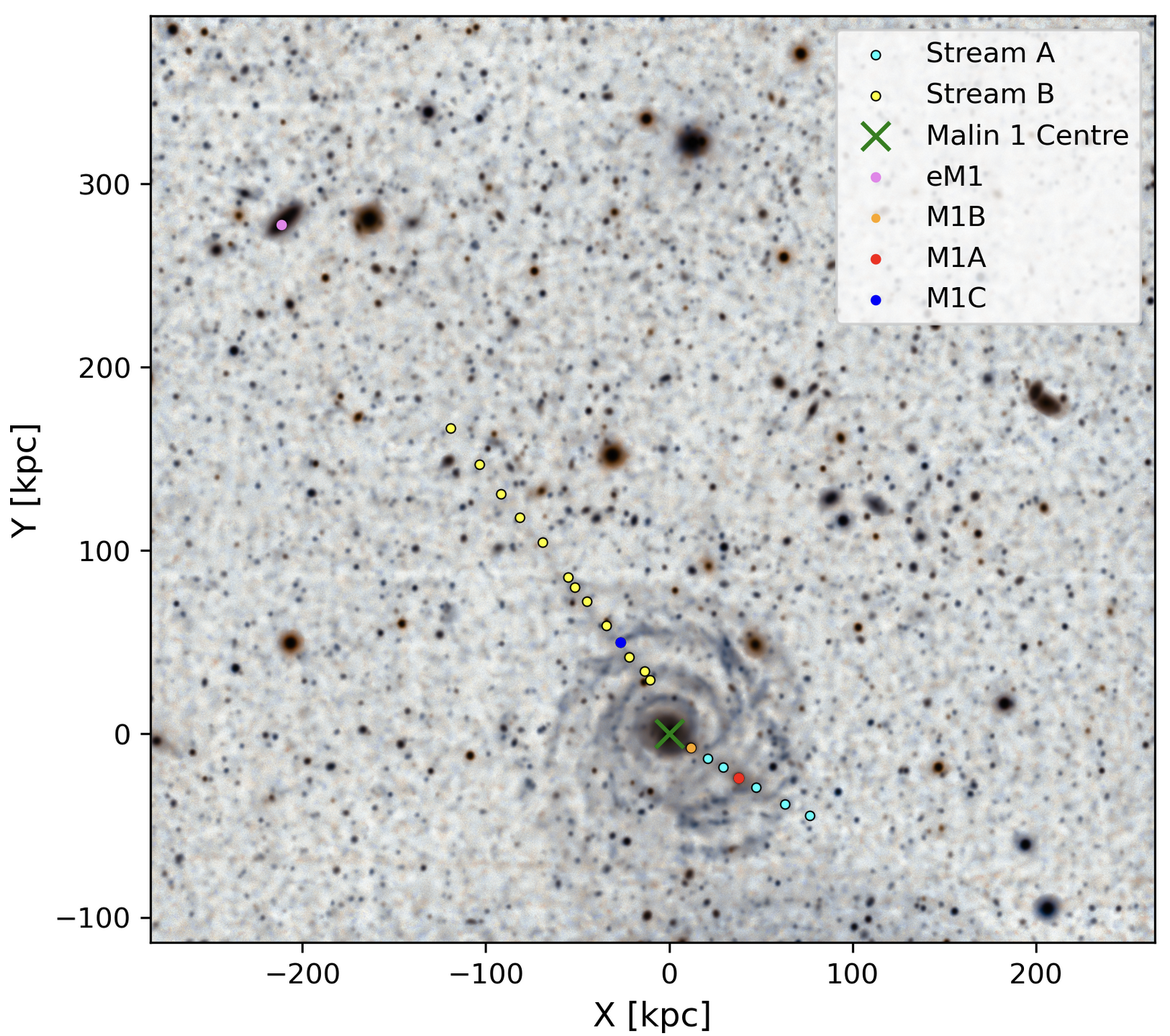
Figure 12: Stream points, sA (cyan points), and sB (yellow points). and four satellites, M1A (red), M1B (orange), M1C (blue), and eM1 (violet). Malin 1 center is mark with a cross (green). Data values are show in Table 6.

To model Malin 1, the surface brightness profile from observations was applied in different bands: $HST/F814W$ for the central area, within $<15$ kpc (Barth, 2007), and the $r$ and $g$ bands for the extended disc, reaching out to $100-120$ kpc in radius (Moore & Parker, 2006; Reshetnikov et al., 2010; Saha et al., 2021). In the analysis, we also used the SB profile of the R-band as explained in Lelli et al. (2010). Furthermore, analysis was conducted on the HI rotational velocity curve, taking into account the stellar, gaseous, and dark matter components. (Pickering et al., 1997; Lelli et al., 2010). Additionally, the coordinates of $x$ and $y$ for the stream points, using the centre of Malin 1 as the inertial reference frame, were determined by photometric analysis (see Fig. 12 and Table 6) and serve as observational data. The $x$-axis aligns with the right ascension ($\alpha$) and increases leftward on the sky plane. The $y$-axis aligns with the declination ($\delta$) and increases northward (upward) in the plane of the sky. The statistical accuracy of each coordinate $x$ and $y$ was enhanced by using the projected angular scale and the median seeing of $0.8$ arcsec (Galaz et al., 2015), given a confidence level of $\pm 1.25$ kpc. For the distance $r$ measured from the centre of Malin 1, error propagation was used (see Fig. 12 and Table 6).

Moreover, the peculiar velocity of the satellite, denoted $V_{\text{Peculiar}}$ and cited from various sources (Dey et al., 2019; Cook et al., 2023; Reshetnikov et al., 2010; Saburova & Cherepashchuk, 2021; Galaz et al., 2015; Junais et al., 2024; Johnston et al., 2024), is listed in Table 3.

Table 3: Peculiar Velocity, $V_{los}$, and related properties of Malin 1 and associated galaxies

Galaxy a	$V_{peculiar}[\mathrm{km/s}]$ b	Petrosian radius [kpc] g	Luminosity [$\mathrm{L_{\odot}}$] h	$M/L$ [$\mathrm{M_{\odot}/L_{\odot}}$] n	$M[\mathrm{M_{\odot}}]$q
M1	0 $\pm$ 1 c	5.6 $\pm$ 0.2	6.0 $\times$ 1010 i	3.4 i	$4.81\times 10^{11}$ r
eM1	$132\pm 37$ d	5.2 $\pm$ 0.4	9.47 $\times$ 109 j	0.9 o	$8.52\times 10^{9}$
M1B	$65\pm 22$ d	2 $\pm$ 2	1.63 $\times$ 109 k	3.4 p	$5.54\times 10^{9}$
M1C	54 $\pm$ 28 e	1.5 $\pm$ 0.5	1.26 $\times$ 108 l	0.9 o	$1.13\times 10^{8}$
M1A	54 f	2 $\pm$ 2	1.12 $\times$ 109 m	3.4 p	$3.81\times 10^{9}$

^a Galaxies abbreviations, defined in Table 2, and in Fig.1.
^b Relative radial velocity of the satellite with respect to Malin 1’s, and the fact that $z<0.1$.
^c M1 centre with dispersion which comes from the projected angular scale (Galaz et al., 2015).
^d Reported by Reshetnikov et al. (2010).
^e (Junais et al., 2024, and private communication).
^f Our estimation based on both, M1A and M1C having approximately the same distance from the M1 centre.
^g Radius where surface brightness is 20$\%$ of the average within it (Petrosian, 1976; Psychogyios et al., 2016); data from SDSS SkyServer (2024).
^h Luminosity in Solar units.
ⁱ Our fitting integrated in $R$ band using the Isothermal profile.
^j Visual $L_{\rm z}$ band (Cook et al., 2023).
^k cE in r band (SDSS SkyServer, 2024).
^l UDG in r band (SDSS SkyServer, 2024).
^m cE in r band (SDSS SkyServer, 2024).
ⁿ Mass to Light ratio in solar units (Bell & De Jong, 2001).
^o M/L value for cE (Bell & De Jong, 2001).
^p M/L value for LSB or UDG (Bell & De Jong, 2001).
^q Stellar mass in solar units.
^r Stellar mass estimation using the Isothermal profile.

3.2 Malin 1 gravitational potential

To investigate the dynamics of Malin 1 satellites, we need to model its gravitational potential to calculate the orbits of its satellite galaxies.

The modelling process involves two primary phases. Initially, we constructed a model of the Malin 1 light profile using HST / F814W photometric data, as detailed in Section 3.1. We leveraged photometric models that offer analytical solutions with the capability to swiftly compute Malin 1’s gravitational field. This facilitates the investigation of an extensive parameter space with innumerable orbital calculations. Specifically, we used a Miyamoto-Nagai potential (Miyamoto N. & Nagai R., 1975), which is ideal for a wide range of mass distributions, from a thin disk to a fully spherical configuration. To represent the bar/bulge substructure, we used one component (Plummer H. C., 1911; Long & Murali, 1992), another for the central disc, and yet another for the external large disk component, both configured with Kuzmin profiles (Binney J. & Tremaine S., 2008). In the subsequent phase, photometric models were utilised to fit gas kinematic observations. For the representation of the dark halo, we implemented both the Navarro-Frenk-White (NFW) profile (Navarro et al., 1996), which aligns with the $\Lambda$CDM model, and a pseudoisothermal profile (De Blok & Bosma, 2002) (refer to Sect. 3.3).

Both profiles are widely used to describe the density distribution of dark matter halos (Lelli et al., 2010; De Blok & Bosma, 2002). NFW assumes that dark mater halos have a characteristic ”cuspy” central density and extend over large distances. The pseudoisothermal profile, on the other hand, features a flat central core, which implies a constant density at the centre (Mo, 2010).

The gravitational potential model proposed by Miyamoto N. & Nagai R. (1975), eq. (1), depending on the choice of the two parameters $a$ and $b$, can represent the potential of an infinitesimally thin disk to a spherical system. For example, when $a=0$, the potential $\Phi_{MN}$ simplifies to the Plummer potential (Plummer H. C., 1911). Conversely, if $b=0$, $\Phi_{MN}$ becomes equivalent to the Kuzmin potential characteristic of a razor-thin disk (Binney J. & Tremaine S., 2008). In our analysis, we combined a Plummer core area profile (Plummer H. C., 1911) with two Kuzmin profiles for the central and peripheral regions of the galaxy (Binney J. & Tremaine S., 2008).

$$\Phi_{MN}(R,z)=-\frac{GM}{\sqrt{R^{2}+\left(a+\sqrt{z^{2}+b^{2}}\right)^{2}}},$$ (1)

In this context, $R=\sqrt{x^{2}+y^{2}}$, denotes the cylindrical radius within the disc’s plane; $x,y,z$, are the spatial coordinates measured in the Malin 1 centre, while $\sqrt{R^{2}+z^{2}}=r$, indicates the radial separation from that centre, as used in Plummer H. C. (1911). The parameters $a$ and $b$ in eq. (1) define the characteristic length scales. The mass parameter, $M$, represents the mass accordinlgly, we call $M\equiv M_{0}$ for the Plummer potential, $M\equiv M_{1}$ for the central region, and $M\equiv M_{2}$ for the galaxy’s outskirts (see Section 3.3). For photometric modelling, we fit the luminosity of each component $L_{x}$. The luminosity can be converted to mass $M_{x}=\gamma_{x}L_{x}$ where $\gamma_{x}$ is the stellar mass-to-light ratio in the band $x$, typically expressed in solar units $M_{\odot}/L_{\odot}$. The value of $\gamma_{x}$ is determined later during the fitting of the rotation curve. This process is often carried out under the maximal disk assumption, which posits that the stellar disk contributes the maximum possible fraction of the observed rotation curve before the dark matter halo becomes dominant. However, for LSB galaxies, including Malin 1, this assumption may not always hold, as such systems are generally dark mater dominated at all radii (Binney J. & Tremaine S., 2008; De Blok & Bosma, 2002).

Moreover, we consider two dark mater profile models to explore the effects of the mass model on the orbital calculations. These correspond to the NFW model (Eq. 2) and pseudoisothermal model (Eq. 3), defined as:

$$\Phi_{NFW}(r)=-\frac{GM_{h}\ln(1+r/r_{s})}{r}\left[\ln(1+c)-\frac{c}{1+c}\right]^{-1},$$ (2)

$$\Phi_{Iso}(r)=-4\pi G\rho_{0}r_{c}^{2}\left[\frac{1}{2}\ln\left(1+\frac{r^{2}}{r_{c}^{2}}\right)+\frac{r_{c}}{r}\tan^{-1}\left(\frac{r}{r_{c}}\right)\right].$$ (3)

In the context of dark mater halos, the NFW model defines the concentration parameter as $c=r_{200}/r_{s}$. Here, $r_{200}$ is the virial radius where the density becomes 200 times the critical density of the Universe, while $r_{s}$ signifies the scale radius of the halo. On the other hand, in the pseudoisothermal profile (De Blok & Bosma, 2002), the parameter $r_{c}$ defines the core radius, and $\rho_{0}$ indicates the central density of the dark matter halo.

The pseudoisothermal profile generally leads to an increased virial mass and radius, due to its flat inner region and slower decline in density, allowing more mass to gather in the halo, which could better suit Malin 1.

In addition, Malin 1 has a HI disk component (Bothun et al., 1987; Pickering et al., 1997). To include this in the gravitational model, we used a Miyamoto-Nagai potential with a mass of $M_{HI}=6.7\times 10^{10}M_{\odot}$ (Lelli et al., 2010), scale length $a_{HI}=a_{2}$, which corresponds to the LSB part of the galaxy, and height $z=0.3\,{\rm kpc}$. This last value is also applied to Kuzmin components. Furthermore, factors 1.1 for molecular $H_{2}$ and 1.4 for helium gas were included (Lelli et al., 2010). Together, these components represent the mass of the baryonic gas.

To maintain conciseness, the abbreviations defined in Table 2 will be used to describe the scenarios presented in Table 4, with additional details provided in Subsec. 3.3. To explore the dynamic properties of Malin 1 satellites, we initially examined their surface brightness profile and rotation curve using mcmc-emcee (Foreman-Mackey et al., 2012; Hogg et al., 2010). These models yield disk parameters that define the galaxy’s mass distribution and gravitational semi-analytical potentials. Following these findings, we performed an orbital analysis with delorean (Blaña et al., 2020), a computational tool designed to reconstruct orbital trajectories based on potential models. This analysis enables the estimation of unknown parameters, including spatial coordinate $z$, tangential velocity $V_{\text{tg}}$, and position angle $\theta$. Furthermore, we determine the pericenter $R_{\text{peri}}$, apocenter $R_{\text{apo}}$, and orbital ellipticity $\epsilon$, facilitating in the characterisation of the movement of satellites and the connection with streams within the galaxy system.

The disk parameters are reported in Table 7, where $a_{0}$, means the Plummer radius, $a_{1}$, and $a_{2}$, are the length scales for the Kuzmin components. $L_{0}$, $L_{1}$, and $L_{2}$, are the corresponding luminosity values for the bulge, central, and LSB parts of the disk.

3.3 Setup for the exploration of scenarios for the progenitor candidates of the stellar streams

In this section, we define different scenarios to identify potential progenitor candidates that have an orbital connection with the observed stellar streams. Studies in the literature about the disruption of satellite galaxies and the formation of stellar streams with N-body simulations typically show that the remaining satellite core has a leading and a trailing component (Fellhauer et al., 2006; Smith et al., 2013, and references therein). Moreover, satellites and their streams can have different morphologies that depend on the potential of the host and, more importantly, on the eccentricity of the orbit. Very circular orbits can produce ring-like streams or polar ring streams, as observed in the Sombrero galaxy (Martínez-Delgado et al., 2021). Radial orbits can produce a more diverse morphology depending on the location where the satellite and the streams are observed in their common orbit. For example, a satellite can be preferentially closer to one of its streams, with the trailing stream being closer to the apocentre and the leading arm could be tidally compressed while entering the host, with the bound core somewhere in the middle of the orbit. (see Fig. 1 in Niederste-Ostholt et al., 2012).

Therefore, we required to consider all detected satellite galaxies near Malin 1 as done in Section 2, and to explore a wide selection of possible scenarios. Table 4 offers a detailed summary of our scenarios, using the abbreviations listed in Table 2. Scenarios include Malin 1 (M1), Malin 1A (M1A), Malin 1B (M1B), Malin 1C (M1C), exo-Malin 1 (eM1), stream A (sA) and stream B (sB). The analysis focusses on scenarios and cases relevant to orbital dynamics and possible progenitor satellites for the streams. Each scenario is evaluated using two distinct gravitational potentials independently applied to Malin 1. As explained in Section 3.2 the models used are the NFW model and the isothermal model. The resulting properties and masses are reported in Section 4.1, but we report a range between $M_{Virial}=1.7\times 10^{12}\,\,{\rm M_{\odot}}$ and $3.8\times 10^{12}\,\,{\rm M_{\odot}}$. Given that the satellite-host mass ratio is small, we model the orbits of the satellites and the streams as test particles where $M_{\rm Satellite}/M_{\rm Malin\leavevmode\nobreak\ 1}<0.01$.

In all cases, orbital calculations of satellite galaxies and stellar streams were performed using an updated version of the software delorean (Blaña et al., 2020), which was combined with emcee and parallel computations to explore a large parameter space and fit observables (Blaña et al. in prep.). This allowed us to explore more than 100 million orbits, including all scenarios, much faster than exploring each scenario with full N-body simulations.

The inputs included stream coordinates, Line-Of-Sight (LOS) velocities, and satellite distances from the Malin 1 centre, shown in Table 6. The outputs consist of spatial coordinates $z$, tangential velocity $V_{\text{tg}}$, Position Angle $\theta$, along with the pericenter $R_{\text{peri}}$, apocenter $R_{\text{apo}}$, and ellipticity $\epsilon$. Some common values for all scenarios are the Virial Ratio range $\eta=[-1,0]$, where $\eta=2KE/PE$, to ensure the negative potential energy needed for the bound satellites. The initial positions and their radial distance from the satellites are shown in Table 6. In all cases, both dark matter profiles, NFW, and isothermal were tested. However, the last one gives us a better fit. The $z$-axis points in the direction of $-V_{\text{los}}$, corresponding to a positive motion along the line of sight through us. So, $v_{z}=-V_{\text{los}}$. The stream points, sA and sB, are shown in Fig. 12 and the values in Table 6.

Table 4: Scenarios and cases regarding orbital dynamics and satellite progenitor candidates for streams. Each scenario has been evaluated using two halo models: the NFW model, and the Isothermal model. The NFW model has $M_{Virial}\approx 1.7\times 10^{12}\,\mathrm{M_{\odot}}$ and $R_{Virial}\approx 247$ kpc, with a concentration parameter $c=10.585$. The Isothermal model considers $M_{Virial}\approx 3.8\times 10^{12}\,\mathrm{M_{\odot}}$ and $R_{Virial}\approx 323$ kpc.

Scenario	Case	Combinations of Progenitor Candidate and Stellar Streams
I	a	eM1 + sB
	b	eM1 + sA + sB
II	a	M1C + sB
	b	M1C + sA + sB
III	a	M1B + sB
	b	M1B + sA + sB
IV	a	M1A + sA
	b	M1A + sA + sB
V	a	sA
	b	sB

We defined five scenarios, with two subcases each, having a total of 10 configurations. These are summarised in Table 4, and are the following:

• Scenario I-a: eM1+sB.
  

  In this Scenario, eM1 and sB constrain the current tangential velocity of eM1 by computing various orbits backward in time. This scenario is interesting because sB seems to connect the M1 centre with the eM1 offset position directly (see region 3 and 4 in Fig.1). To explore the radial and polar orbits, we used the following ranges: first $[-13.0,20.0]$ Gyr and next $[9.0,3.7]$ Gyr, $z\in[-800,-300]$ kpc, and $z\in[-343,0]$ kpc. Tangential velocity values that would lead to eM1’s orbit that entered and left Malin 1’s dark halo (Deason & Belokurov, 2024). So, for both situations, a tangential velocity $V_{\text{tg}}\in[0,1000]$ km/s, and $\theta\in[0^{\circ},90^{\circ}]$, covering the natural direction of eM1. For this analysis, a mcmc-emcee approach was employed to estimate parameter uncertainties. The configuration involved the number of walkers, $n_{\text{walkers}}=797$, steps, $n_{\text{steps}}=2997$. All to ensure robust convergence. The observed radial and positional data for eM1 is: radial distance $R=350.0$ kpc and LOS velocity $V_{\text{los}}=132$ km/s (Reshetnikov et al., 2010). The eM1 coordinates are $x=-211.38$ kpc, $y=277.78$ kpc, with $v_{z}=-V_{\text{los}}$.

• Scenario I-b: eM1+sB+sA.
  

  It is possible that both streams, sA and sB, originated from eM1, with sA forming first, followed by sB. The following constraints were applied to explore this hypothesis: a $z$ range of $z\in[-800,-300]\,\text{kpc}$, and a tangential velocity between $v_{t}\in[0,1000]\,\text{km/s}$ and $\theta\in[0^{\circ},360^{\circ}]$.

• Scenario II-a: M1C+sB.
  

  The origin of stream sB remains uncertain. A fascinating hypothesis is that M1C could have generated both the forward and backward segments of sB, indicating that the observed stream might be undergoing a degenerative process. This hypothesis suggests that the leading and trailing segments are observable, with M1C core placed, as seen in other systems (Niederste-Ostholt et al., 2012; Bonaca et al., 2021). To investigate this, orbital calculations were carried out in both temporal directions - forward (leading) and backward (trailing) - for M1C. Various parameter ranges for $z$, $v_{t}$, and $\theta$ were used. These included $z\in[-43,-0]\,\text{kpc}$, along with a tangential velocity of $v_{t}\in[300,500]\,\text{km/s}$ and an angular direction $\theta\in[0^{\circ},360^{\circ}]$.

  The initial configuration mcmc-emcee involved the following settings: $n_{\text{walkers}}=170$, $n_{\text{steps}}=1300$, $\text{discard}=0.2$, $\text{samplefr}=1$, with an integration time $[-0.5,0.3]$ Gyr, to ensure the study of the degenerative process. $\eta=$ -1.0 due a bigger negative potential energy would be needed for M1C. The observed radial, LoS velocity and positional data for M1C is $R=14$ kpc, $V_{\text{los}}=54$ km/s (Junais et al., 2024, and private communication), and $x=-21.96$ kpc, $y=41.80$ kpc, with $v_{z}=-V_{\text{los}}$.

• Scenario II-b: M1C+sB+sA.
  Here we continue our hypothesis that M1C could have generated not only the forward and backward segments of sB, but the possible connection between both streams, sA and sB, with M1C as the progenitor. To search for this possibility, the initial setup for the parameter ranges is $z\in[-100,0]\,\text{kpc}$, along with a tangential velocity of $v_{t}\in[0,570]\,\text{km/s}$ and an angular direction $\theta\in[0^{\circ},360^{\circ}]$. For mcmc-emcee involved, $n_{\text{walkers}}=400$, $n_{\text{steps}}=1300$, $\text{discard}=0.2$, with an integration time $[-0.5,0.3]\,\text{Gyr}$, to ensure the study of the degenerative process. The observed radial, LoS velocity, and positional data for M1C are the same as in Scenario II-a.

• Scenario III-a: M1B + sB.
  

  This scenario is particularly interesting, as it explores M1B as the possible progenitor of sB. Therefore, sB might consist of debris from stars and gas that once belonged to the compact elliptical M1B. This investigates tangential velocity values that would lead to M1B orbit inside the Malin 1 dark halo. The parameter ranges include a spatial range $z\in[-43,43]$ kpc, a tangential velocity $V_{\text{tg}}\in[0,400]$ km/s, and $\theta\in[0^{\circ},360^{\circ}]$, covering all spatial orientations. The setup of mcmc-emcee is $n_{\text{walkers}}=197$, $n_{\text{steps}}=900$, $\text{discard}=0.2$, integration time $[0,[-6.7,1.3]\text{Gyr}$. The observed radial, LoS velocity, and positional data for M1B is $R=14$ kpc, $V_{\text{los}}=54$ km/s (Junais et al., 2024, , and private communication), and $x=11.93$ kpc, $y=,-7.65$ kpc and $v_{z}=-V_{\text{los}}$.

• Scenario III-b: M1B + sA + sB.
  

  This scenario investigates the possible connection between streams sA and sB with M1B as progenitor.

  To investigate this, orbital calculations were carried out in both temporal directions - forward (leading) and backward (trailing) - for M1B. $z\in[-71,0]\,\text{kpc}$, along with a tangential velocity of $v_{t}\in[0,999]\,\text{km/s}$ and an angular direction $\theta\in[0^{\circ},90^{\circ}]$. The configuration mcmc-emcee involved the following settings: $n_{\text{walkers}}=397$, $n_{\text{steps}}=1300$, with an integration time $[-7.5,7.5]\text{ Gyr}$, to place M1B at the core of the degenerative process stream. Observational data are the same as Scenario III-a.

• Scenario IV-a: M1A+sA.
  

  In this scenario, look for an orbit in which M1A is the progenitor of sA. Upon a review of the Milky Way streams (Niederste-Ostholt et al., 2012), one can see that they go perpendicular to the galactic plane. So, we have the possibility that sA is continuing this situation. This hypothesis says that M1A could be responsible for sA. To investigate this, orbital simulations were conducted applying the following parameters tested, which included $z\in[-243.0,0.4]\,\text{kpc}$, along with a tangential velocity of $v_{t}\in[0,500]\,\text{km/s}$ and an angular direction $\theta\in[0^{\circ},360^{\circ}]$.

  The mcmc-emcee configuration involved the following settings: $n_{\text{walkers}}=397$, $n_{\text{steps}}=977$, with an integration time $[-1.7,0.4]\,\text{Gyr}$. The LoS velocity was adopted as the same as M1B, that is, $V_{\text{los}}=54$ km / s (Junais et al., 2024, , and private communication).

• Scenario IV-b: M1A+sA+sB.
  

  In this scenario, we explore the same origin for both sA and sB. A compelling hypothesis is that M1A could be responsible for the leading and trailing parts of sA and be in some way connected to sB. This hypothesis suggests that the leading and trailing segments are observable, with M1A core placed, as seen in other systems (Niederste-Ostholt et al., 2012; Bonaca et al., 2021). To investigate this, various parameter ranges for $z$ were employed. These included $z\in[-13,0]\,\text{kpc}$, along with a tangential velocity of $v_{t}\in[350,500]\,\text{km/s}$ and an angular direction $\theta\in[0^{\circ},360^{\circ}]$. The configuration mcmc-emcee involved the following settings: $n_{\text{walkers}}=397$, $n_{\text{steps}}=597$, with an integration time $[-0.7,3.0]\,\text{Gyr}$, to ensure the study of the degenerative process.

• Scenario V-a: sA. The progenitor was destroyed.
  

  In this scenario, a possible origin of sA is explored. The hypothesis is that sA could be a fingerprint of the history of assembly of a galaxy (Deason et al., 2023; Panithanpaisal et al., 2021). To investigate this, orbital calculations were carried out in a leading integration. Parameter ranges for $z\in[-10,0]\,\text{kpc}$, along with a tangential velocity of $v_{t}\in[300,700]\,\text{km/s}$ and an angular direction $\theta\in[180^{\circ},270^{\circ}]$. The configuration mcmc-emcee involved the following settings: $n_{\text{walkers}}=397$, $n_{\text{steps}}=1700$, with an integration time $[-7.5.,0.3]\text{Gyr}$. The closest sA point to M1 was taken as a focus point in the analysis, with $x=-11.93$ kpc, $y=-7.65$ kpc, and we include $z=0.01$ to define the spatial position for this case.

• Scenario V-b: sB. The progenitor was destroyed.
  In this final scenario, another possibility of a destruction event is examined. The hypothesis is that the progenitor sB might be dismantling the satellite galaxy through gravitational tidal forces (Panithanpaisal et al., 2021). Hence, it is plausible that we observe signs of the disintegration process of the progenitor sB. To delve into this, orbital computations were performed using forward(leading) integration. Various values for $z$ were studied to examine planes both above and below the galaxy. These values included a tangential velocity of $v_{t}\in[500,900]\,\text{km/s}$ and an angular direction $\theta\in[0^{\circ},90^{\circ}]$. The mcmc-emcee configuration used the following parameters: $n_{\text{walkers}}=397$, $n_{\text{steps}}=1997$, and an integration time $[-0.3,0.4]\,\text{Gyr}$. LOS velocity $V_{\text{los}}\approx 54$ km / s was chosen using a similar value of point C in sB (Junais et al., 2024). The coordinates of the closest sB point to M1 were $x=-10.61$ kpc, $y=29.37$ kpc, $z=-24.22$ kpc. The last component $z$ was calculated as the projection over the galactic plane. And $v_{z}=-V_{\text{los}}$.

The results are shown in Section 4.2.

4 Results

In the first part, we report our results on the light and potential modelling of Malin 1. Then we proceed to report on our modelling of the stellar streams. Lastly, a ranking was proposed together with some practical physical calculations.

4.1 Mass and potential models for Malin 1

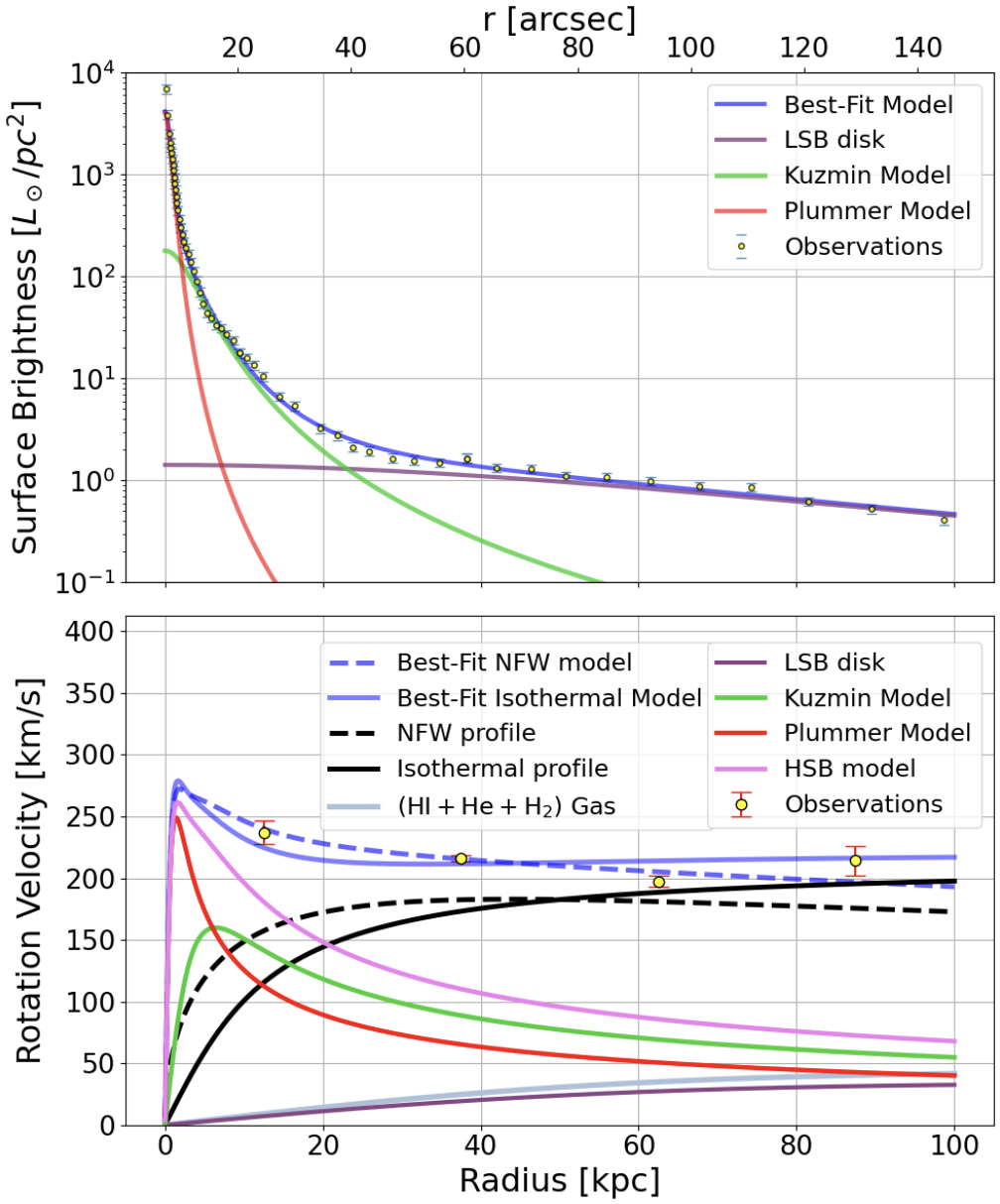
Figure 2: Top panel: shows the observed surface brightness data in the R band (Lelli et al., 2010). In addition we show our fits of a Plummer and a Miyamoto-Nagai (Kuzmin) profiles for the central region and another Miyamoto-Nagai profile for the LSB disk component. Bottom panel: shows the observed HI rotation curve (Lelli et al., 2010). We also show the models fitted photometrically (Plummer and two Miyamoto-Nagai) for the stellar component, and a Miyamoto-Nagai disk for the gaseous component. We also show the fitted dark matter halo models NFW and pseudoisothermal.

The surface brightness profile and the rotation curve fitting were analysed using mcmc-emcee, and are shown in Fig. 2, upper and bottom panels, respectively. The best-fit parameters derived here were later used as input for orbital analysis with delorean (Blaña et al., 2020), to estimate unknown variables, the spatial dimension $z$, the tangential velocity $V_{\text{tg}}$, and the position angle $\theta$. Furthermore, the pericenter $R_{\text{peri}}$, the apocenter $R_{\text{apo}}$, and the ellipticity $\epsilon$ are calculated.

In the upper panel of Fig. 2, we display R band data points as reported by Lelli et al. (2010). The diagram exhibits a Plummer profile that represents the galaxy’s core, along with two separate Kuzmin profiles, one characterising the central area and another for the outskirts, to simulate the LSB disk of the galaxy. In addition, the figure displays the Best-Fit model.

The bottom of figure 2 presents the rotation velocity fitting for two dynamical models, NFW and pesudo-isothermal dark matter profiles. The four $HI$ data points were obtained by Lelli et al. (2010); Pickering et al. (1997). The diagram dissects various components, including the Plummer and Kuzmin models, which describe the core and peripheral sections of galaxies, as well as the gas constituents $HI$, He, and $H_{2}$. It also considers both High- and Low-Surface Brightness regions (HSB and LSB) and includes two dark mater halo models: the NFW model and the pseudoisothermal.

Figure 3 illustrates the optimised emcee fit parameters for the surface brightness model, while Figure 4 shows the equivalent parameters for the rotation curve model. The data compiled for the two profiles is presented in Tables 7. In particular, the key parameters include the following. $L_{0}$ = $1.25^{+0.06}_{-0.06}\times 10^{10}\,L_{\odot}$, $L_{1}$ = $2.33^{+0.07}_{-0.07}\times 10^{10}\,L_{\odot}$, $L_{2}$ = $7.1^{+0.6}_{-0.5}\times 10^{10}\,L_{\odot}$, $a_{0}=1.00^{+0.05}_{-0.05}\,\text{kpc}$, $a_{1}=4.6^{+0.3}_{-0.3}\,\text{kpc}$, and $a_{2}=94^{+7}_{-6}\,\text{kpc}$. An important factor affecting the accuracy of mass modelling is the exact value of stellar mass-to-light ratios (denoted $\Upsilon$). $\Upsilon_{NFW}\simeq 3.2$ $\Upsilon_{\odot}$ for the NFW dark matter halo and $\Upsilon_{Iso}\simeq 3.4$ for the isothermal dark matter halo, in good agreement with Lelli et al. (2010). For the Malin 1 NFW halo, the parameters are $M_{h}(r_{200})=1.7\times 10^{12}\,\,{\rm M_{\odot}}$, $r_{200}=246\,\text{kpc}$, and $l_{s}=22^{+6}_{-3}\,\text{kpc}$, resulting in a concentration of $c_{200}=10.585$. The Malin 1 pseudo-isothermal halo parameters include the density of the central halo, $\rho_{0}=8.8363\times 10^{6}\,{\rm M_{\odot}}\,{\rm pc}^{-3}$ and the radius of the core of the halo, $r_{c}=9.738$, $\,{\rm kpc}$.

Following Barth (2007), we distinguished between High-Surface Brightness (HSB) and Low-Surface Brightness (LSB) galaxies based on their central surface brightness, adopting the common threshold of $\mu_{B}=23.0\,\text{mag arcsec}^{-2}$ (Impey & Bothun, 1997). Using these parameters, we were able to examine the orbital solutions belonging to the various scenarios depicted in Section 3.3. For each scenario, we utilized both NFW and isothermal halo models to determine orbital solutions and discovered that the outcomes did not vary significantly.

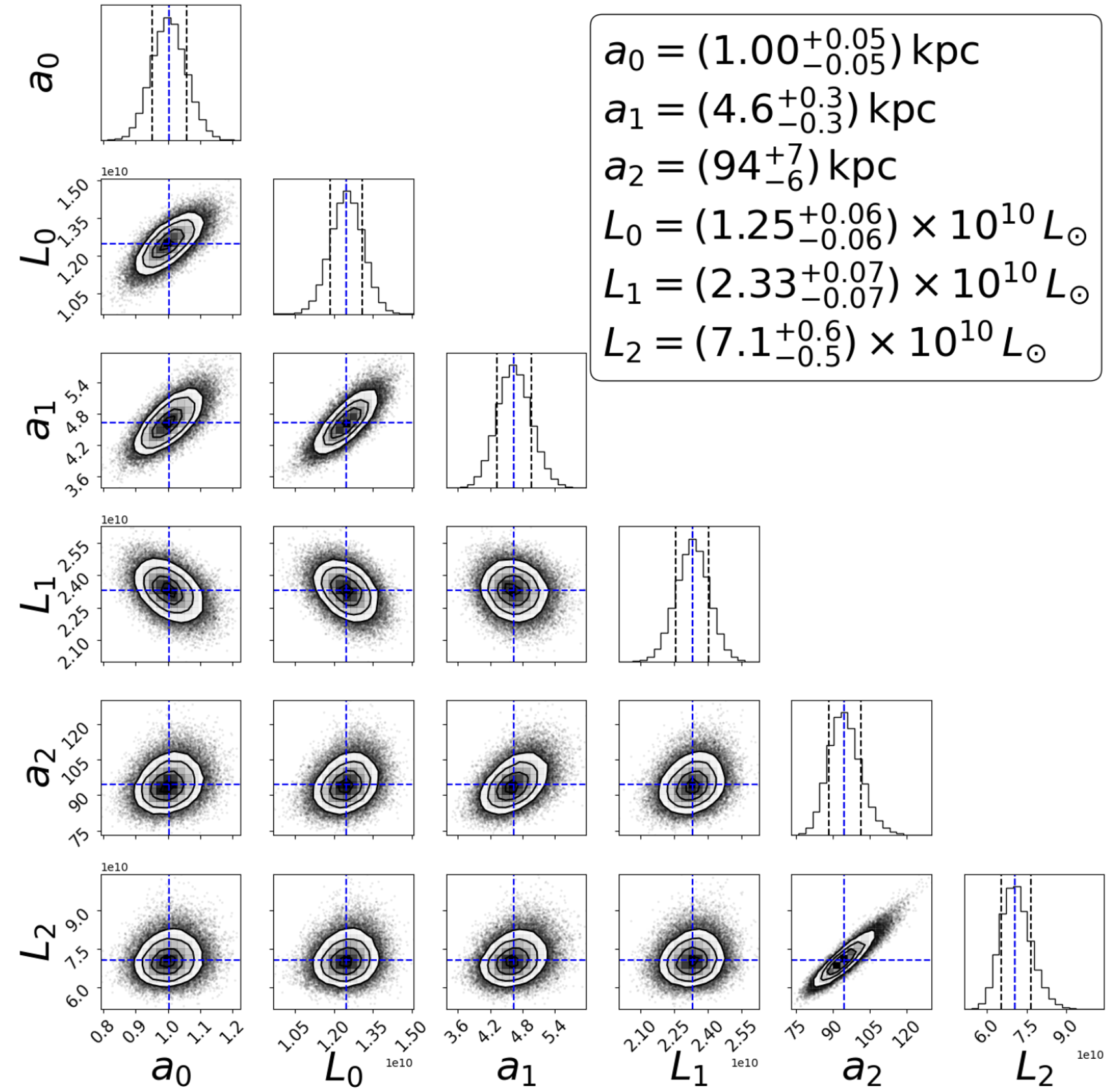
Figure 3: The posterior distributions and covariances for the optimal parameters derived from the emcee-mcmc analysis regarding surface brightness fitting are presented (see Fig. 2, upper panel). These parameters pertain to the model, where $a_{0}$, $a_{1}$, and $a_{2}$ denote characteristic length scales, and $L_{0}$, $L_{1}$, $L_{2}$ represent the measured luminosities in each segmented region of the SB: Plummer for the central region, a Kuzmin profile for the medium section, and another Kuzmin profile for the LSB or peripheral areas. The diagonal histograms reflect the marginalized distributions for each parameter, with vertical dashed lines marking the 16th, 50th, and 84th percentiles (approximately 1-sigma uncertainties), while the contour plots illustrate the covariances between parameter pairs. The peak of each histogram indicates the parameter’s most likely value. The legend outlines the optimal parameter estimates along with their uncertainties, which are essential to the model of the galaxy’s surface brightness.

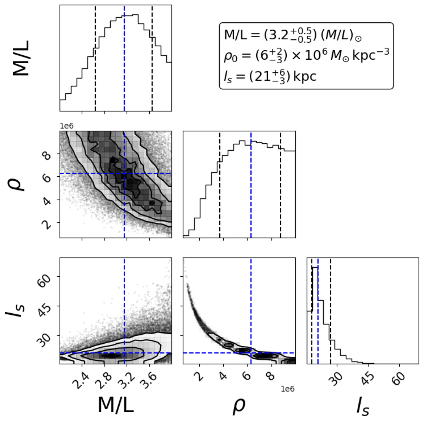
Figure 4: The emcee-mcmc analysis of the rotation curve fitting (Figure 2, lower panel) using the NFW profile, provides posterior distributions and covariances for parameters such as the mass-to-light ratio $(M/L)$, central density $\rho$, and scale length $l_{s}$. On the diagonal, histograms display the marginalized distributions for each parameter, with vertical dashed lines marking the 16th, 50th, and 84th percentiles (approximately $1\sigma$ uncertainties). The contour plots depict the covariances, illustrating parameter correlations. The legend presents the best-fitting parameter values and their uncertainties, which are crucial to the galaxy’s rotation curve model.

4.2 Possible progenitor candidates of the stellar streams and findings

In this study, we detail the results of our orbital fitting procedures applied to both stellar streams and satellite galaxies. Using delorean, we investigated around 10 million orbits per scenario, which is a comprehensive analysis of 100 million orbits. This included two configurations for the Malin 1 potential, encompassing both radial and circular orbits, along with evaluations of bound and unbound orbits, and energy evaluations through the virial ratio. Here, we highlight the solutions that most accurately correspond to the observational data and adhere to physical constraints, such as having bound orbital solutions. However, unbound solutions were also found.

From the ten scenarios analysed, a preliminary classification is as follows.

• Present a progenitor: Ia, IIIa, IVa and Va.

• Progenitor destroyed: Va, and Vb.

• Two streams linked: IIb.

• Unbound orbit: Ib, IIIb, and IVb.

Here we discuss the main physical parameters obtained from the modelling in each scenario.

• Scenario I-a: eM1 + sB. subcases:, eM1 + sB - radial, and eM1 + sB - polar
  For only this scenario we will study two orbital solutions: a radial orbit known here as Scenario I-a-radial, depicted in Fig. 5 and a polar orbit known as Scenario I-a-polar, depicted in Fig. 6. The motivation lies in our quest to identify both radial solutions, where the stellar streams are either converging towards or diverging from the center of Malin 1, experiencing the most intense tidal forces, as well as polar solutions, similar to those observed in the Sombrero galaxy (Martínez-Delgado et al., 2021).
  

  Fig. 5 (Scenario I-a-r), panel i) shows the best radial orbit fit, integrated $[-13.0,20.0]$ Gyr into the optical image of Malin 1 and its surroundings (Galaz et al., 2015). This path links eM1 (denoted by a red star) with stellar stream B (marked by magenta crosses) after making a pass near the Malin 1 disc. For this orbit, the pericenter crossing of eM1 occurred approximately $-1.3$ Gyr ago. The colour bar illustrates the LoS velocities along the orbit, with a maximum variation of $\Delta V_{\text{LoS}}\approx 500$ km/s. This suggests that sB might be associated with eM1, as the trailing segment that was stripped from eM1 in their passage. Panel ii) Shows the plot of distance versus time and velocity versus time shows the satellite’s motion around Malin 1. The maximum likelihood of the pericenter and the velocity was found at about $41$ kpc and $|V|\approx 587$ km/s, respectively, which happened $\sim-1.3$ Gyr ago. Panel iii) Shows the X-Z and Y-Z planes of the orbit. Panel iv) Corner plots show the likelihood distribution of all orbits, the optimal fit parameters in the $50\%$ percentile are $z\sim-8$ kpc, $v_{t}\sim 532$ km/s, PA$\sim 39^{\circ}$. Panel v) The maximum likelihood probability showing a pericentre of $R_{\text{peri}}\sim 465$ kpc and an apocentre of $R_{\text{apo}}\sim 4995$ kpc and $\epsilon\sim 0.44$.

  Fig. 6 (Scenario I-a-p), panel i), presents the best polar orbit. It was integrated $[-9.0,3.7]$ Gyr into the optical image of Malin 1 and its surroundings (Galaz et al., 2015). This path links eM1 (denoted by a red star) with stellar stream B (marked by magenta crosses) after making a pass near the Malin 1 disc. For this orbit, the pericenter crossing of eM1 occurred approximately $-1.3$ Gyr ago, approximately the same time found in the radial orbit, shown in Fig.5, however, with a different pericenter value. The colour bar illustrates the LoS velocities along the orbit, with a maximum variation of $\Delta V_{\text{LoS}}\approx 350$ km/s. This suggests that sB might be associated with eM1 through a polar orbit. Panel ii) plots distance versus time and velocity versus time. The pericenter and velocity were found at about $193$ kpc and $|V|\approx 370$ km / s, respectively, which occurred $\sim 1.3$ Gyr ago. Panel iii) Shows the X-Z and Y-Z planes, and confirm a polar orbit. From the likelihood distribution of all orbits (not shown), the optimal fit parameters in the $50\%$ percentile are $z\sim-8$ kpc, $v_{t}\sim 532$ km/s, PA$\sim 39^{\circ}$, with the model with maximum likelihood probability showing a pericentre of $R_{\text{peri}}\sim 357$ kpc and apocentre of $R_{\text{apo}}\sim 4774$ kpc and $\epsilon\sim 0.47$.

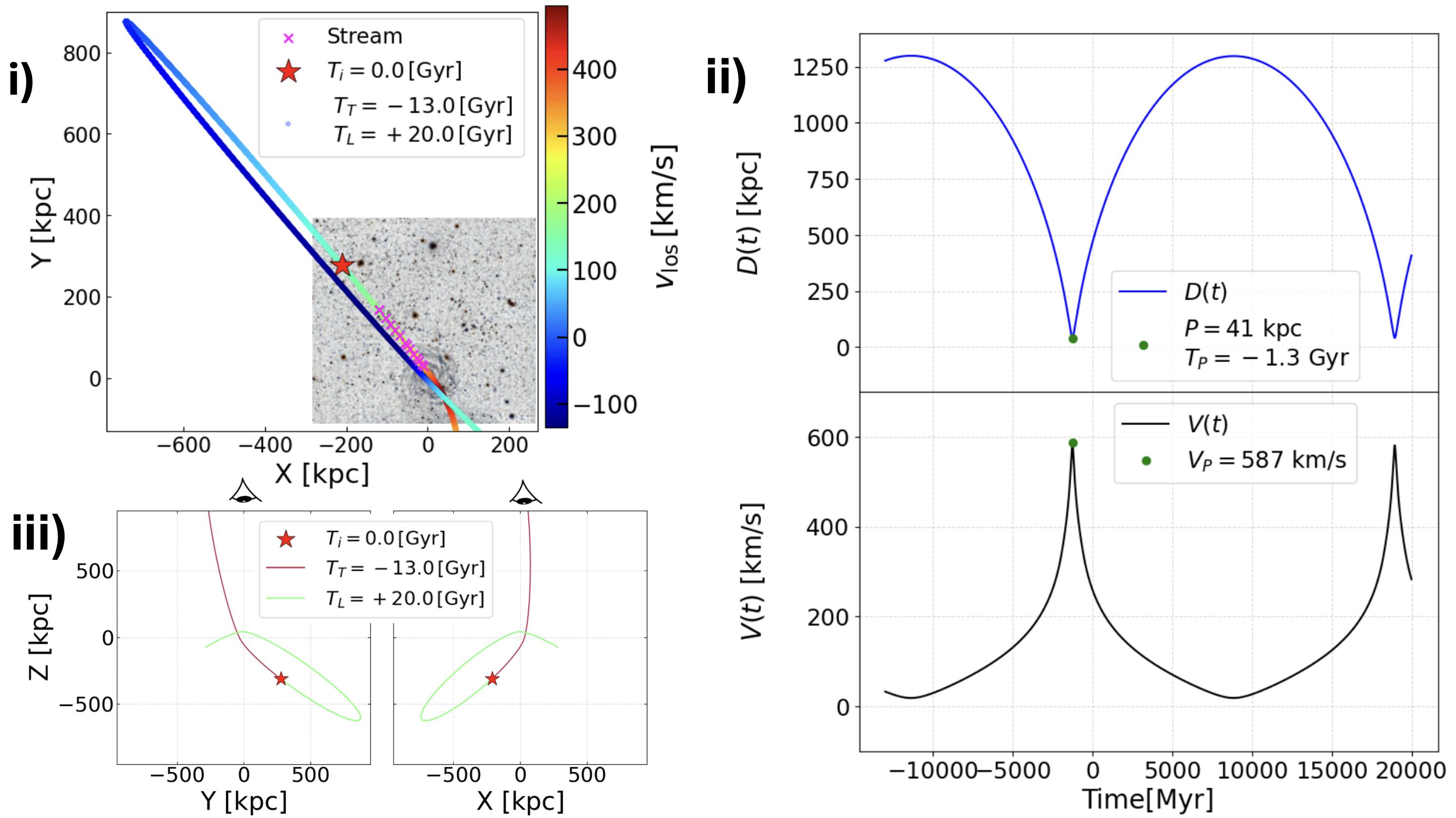
Figure 5: Scenario I-a (radial): eM1+sB-radial. Panel i) A possible radial orbit integrated $[-13.0,20.0]$ Gyr over the optical image of Malin 1 and its environment (Galaz et al., 2015) that connects eM1 (red star) with the stellar stream B (magenta crosses) in the first passage by the Malin 1 disc. For this orbit, the pericenter passage of eM1 was $\sim-1.3$ Gyr ago. The color-bar shows the LOS velocities along the orbit, having a maximum difference of $\Delta V_{\text{LoS}}\approx 500$ km/s. This could be that sB are the trailing part of eM1 as the progenitor. Legend shows stellar stream mark, the time for the progenitor (eM1), denoted ($T_{i}$), and the Trailing ($T_{T}$) and Leading ($T_{L}$) stream times with a common dot for both showing the colour or velocity of eM1 in that moment of the orbit. The isothermal profile was employed for the dark matter. Panel ii) Distance vs time plot and Velocity vs time illustrating the satellite’s kinematics around Malin 1. Pericenter and velocity maximum likelihood were obtained at $\approx 41$ kpc and $|V|\approx 587$ km/s. Panel iii) X-Z and Y-Z orbital planes. The observer would be located at the top of these subpanels, at positive Z and X, Y = (0, 0) kpc is the Malin 1 center. Legend shows the time for the progenitor, $T_{i}=0$ Gyr (present), and the Trailing, in purple colour, ($T_{T}=-13$ Gyr) and the Leading, in light green colour, ($T_{L}=20$ Gyr). The best orbit has $z\sim-8$ kpc, $v_{t}\sim 532$ km/s, $\mathrm{PA}\sim 39^{\circ}$, $R_{\text{peri}}\sim 465$ kpc, $R_{\text{apo}}\sim 4955$ kpc, and $\epsilon\sim 0.44$.

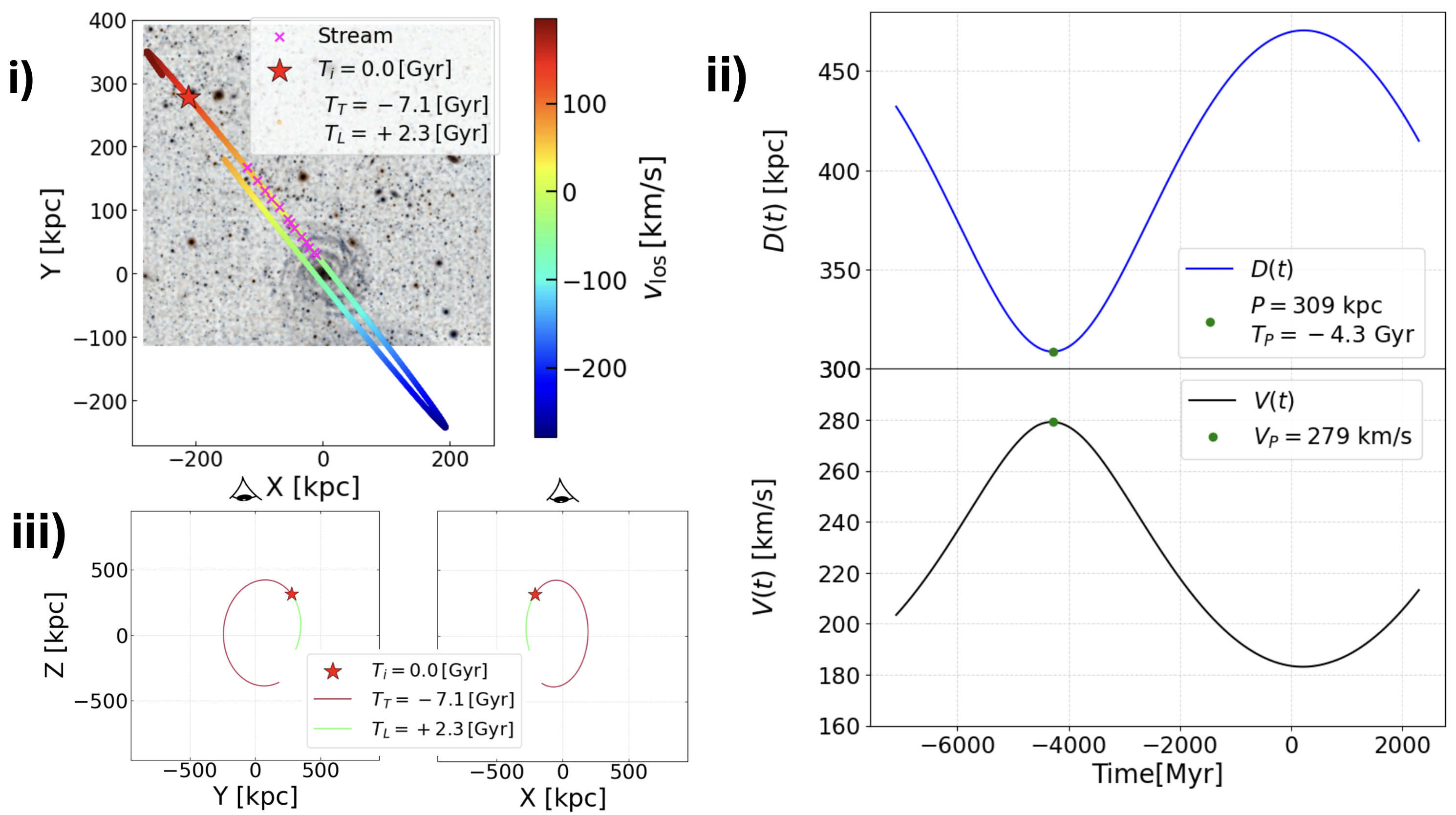
Figure 6: Scenario I-a (polar): eM1+sB-polar. Panel i) A possible polar orbit integrated $[-9.0,3.7]$ Gyr over the optical image of Malin 1 and its environment (Galaz et al., 2015) that connects eM1 (red star) with the stellar stream B (magenta crosses) in the second passage by the Malin 1 disc. For this orbit, the pericenter passage of eM1 was $\sim-4.3$ Gyr ago. The color-bar shows the LOS velocities along the orbit, having a maximum difference of $\Delta V_{\text{LoS}}\approx 350$ km/s. This could be that sB are the trailing part of eM1 as the progenitor. Legend shows stellar stream mark, the time for the progenitor (eM1), denoted ($T_{i}$), and the Trailing ($T_{T}$) and Leading ($T_{L}$) stream times with a common dot for both showing the colour or velocity of eM1 in that moment of the orbit. The isothermal profile was employed for the dark matter. Panel ii) Distance vs time plot and Velocity vs time illustrating the satellite’s kinematics around Malin 1. Pericenter and velocity maximum likelihood were obtained at $\approx 193$ kpc and $|V|\approx 370$ km/s. The best orbit has $z\sim-8$ kpc, $v_{t}\sim 532$ km/s, PA$\sim 39^{\circ}$, $R_{\text{peri}}\sim 357$ kpc, $R_{\text{apo}}\sim 4455$ kpc, and $\epsilon\sim 0.47$. Panel iii) X-Z and Y-Z orbital planes. The observer would be located at the top of these subpanels, at positive Z and X, Y = (0, 0) kpc is the Malin 1 center. Legend shows the time for the progenitor, $T_{i}=0.0$ Gyr (present), and the Trailing, in purpple colour, ($T_{T}=-7.1$ Gyr) and the Leading, in light green colour, ($T_{L}=2.3$ Gyr). We can see an equivalent stellar stream like the one around the Sombrero galaxy (Martínez-Delgado et al., 2021).

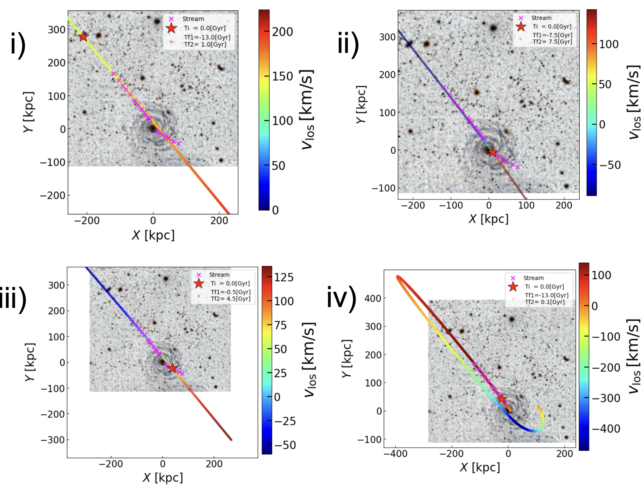
Figure 13: Unbound orbits: panel i) Scenario I-b: eM1+sB+sA, panel ii) Scenario III-b: M1B+sB+sA, and panel iii) Scenario IV-b: M1A+sA+sB. Panel iv) Scenario II-a: M1C + sB, solution contained in Scenario II-b: M1C + sB + sA, as shown in Fig. 7.

• Scenario I-b: eM1 + sB + sA.
  In our search for a radial orbit or approximation to it, a confirmed apparently unbound orbit was found. The pericentric passage is elevated, $575$ kpc with a velocity of $660$ km/s which happened $0.77$ Gyr ago. A radial orbit was not possible to find to fit both streams simultaneously. The unbound orbit is shown in panel i) Fig. 13.

• Scenario II-a: M1C + sB.

  This scenario explores M1C as the progenitor of sB, suggesting that sB might contain leftover stars and undetected gas that were once linked to M1C. The detailed examination of one probable orbit is presented in panel iv) in Fig. 13, integrated over $[-13.0,0.1]$ Gyr, illustrating potential stream disintegration in both trailing and leading sections in sB (indicated by magenta crosses), with M1C (marked by a red star) at the core of sB. It experienced a pericentre passage $\sim 9$ Gyr ago, currently it would be approaching for the second time, currently entering Malin 1. This scenario would naturally explain the formation of the sB stream in the past encounter $9$ Gyr when M1C had its first in-fall. Currently, the stream and M1C would be under tidal compression as it approaches Malin 1. The orbit overlayed on the optical image of Malin 1 and its peripheries (Galaz et al., 2015). The colour bar shows LOS velocities that can reach $\Delta V_{\text{LoS}}\approx 500$ km/s, indicating significant dynamic interactions over time. Interestingly, this scenario has been reached also in scenario II-b explained to continuation.

• Scenario II-b: M1C + sB + sA.
  This setup investigates the possible link between both streams, sA and sB, with M1C as the progenitor. This suggests that sA and sB may be composed of stellar remnants formerly associated with M1C. Figure 7 illustrates the proposed orbit and its examination in three different panels. Panel i) Displays an example of an integrated orbit over $[-0.5,3.0]$ Gyr, illustrating the best-fitted orbit showing a possible stream disintegration in both the trailing and leading sections (indicated by magenta crosses). M1C is marked by a red star in the centre of sB. In this possible tidally disrupting system, both the leading and the trailing arms cover both streams, as illustrated by Niederste-Ostholt et al. (2012). The orbit overlayed on the optical image of Malin 1 and its peripheries (Galaz et al., 2015). The colour bar shows LoS velocities that can reach $\Delta V_{\text{LoS}}\approx 400$ km/s. Panel ii) The distance versus time plot outlines the orbital movement of the satellite. The pericenter value $\sim 3$ kpc and a velocity magnitude of approximately $|V|\sim 736$ km / s occurred with the leading arm $\sim 2.3$ Gyr. Panel iii) X-Z and Y-Z planes of the orbit. For the corner plots (not displayed) the optimal parameters are $z\sim-64$ kpc, $v_{t}\sim 378$ km/s, PA$\sim 217^{\circ}$, with orbital characteristics that include a periapsis around $R_{\text{peri}}\sim 49$ kpc, an apoapsis of $R_{\text{apo}}\sim 296$ kpc, and an ellipticity $\epsilon\sim 0.30$. Interestingly, Scenario I-b was reach in the first passage.

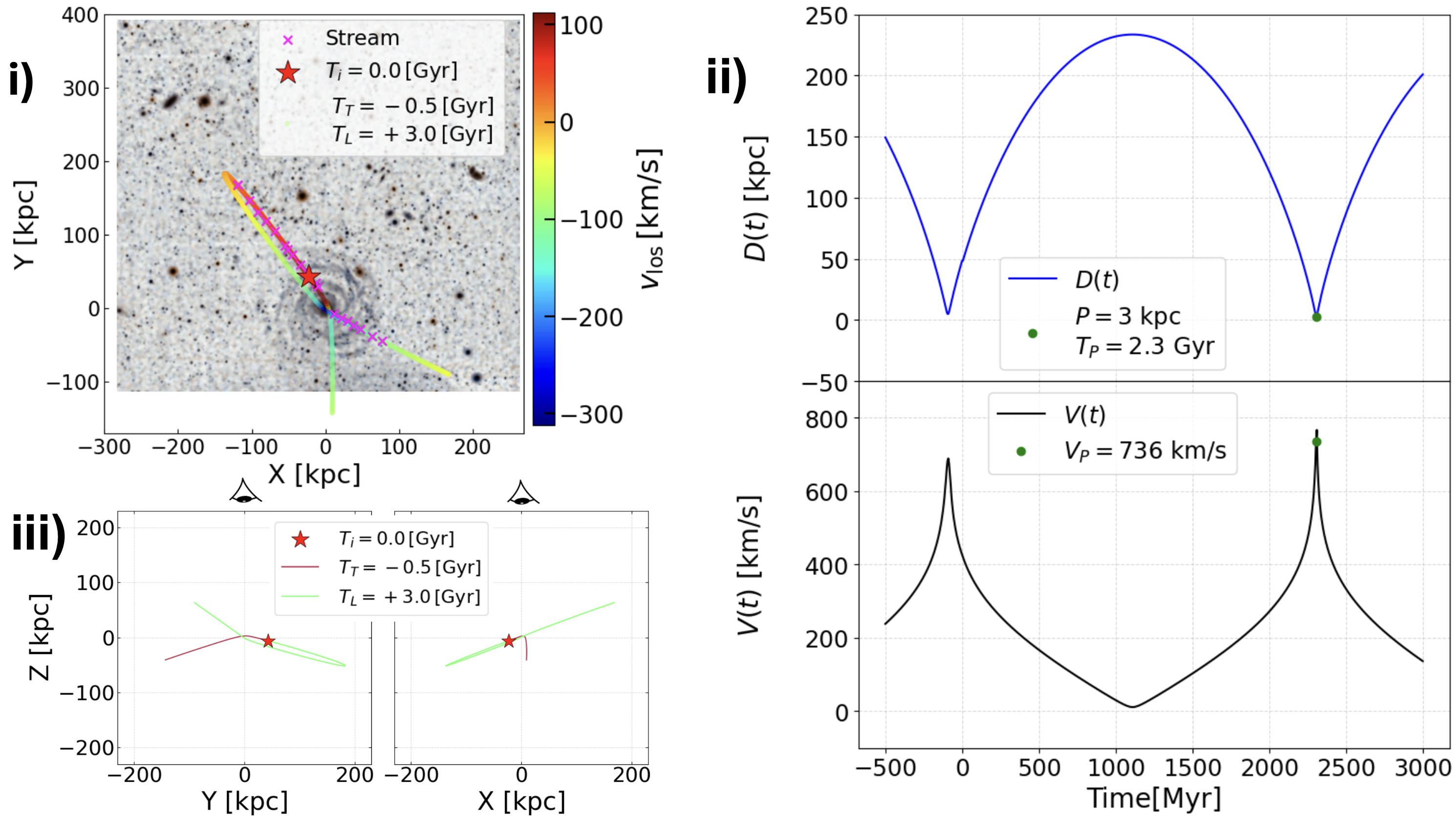
Figure 7: Scenario II-b: M1C+sB+sA. Panel i) An example of an orbit integrated over $[-0.5,3.0]$ Gyr show not only a possible association of the stream in their trailing and leading parts in sB shown by magenta crosses with M1C represented by a red star in the core, but also the orbit connects sA in the second pericenter passage. It is superimposed on the optical image of Malin 1 and its surroundings (Galaz et al., 2015). The color-bar illustrates LoS velocities along the orbit, having a maximum difference of $\Delta V_{\text{LoS}}\approx 500$ km/s. This could be that both components of sB shows the trailing and leading stream components with M1C as the progenitor. In addition, the leading shows a link with sA. Legend shows stellar stream mark, the time for the progenitor (M1C), denoted (Ti), and the Trailing ($T_{T}$) and Leading ($T_{L}$) times with a common dot for both showing the colour or velocity of M1C at that specific moment of the orbit. The isothermal profile was employed for the dark matter. Panel ii) Distance vs time, and a magnitude velocity vs time with $|V|\approx 736$ km/s. In this orbit, the trailing pericenter passage of M1C occurred approximately $-0.1$ Gyr ago, and $2.3$ Gyr for the leading arm. Panel iii) X-Z and Y-Z orbital planes. The best orbit has $z\sim-64$ kpc, $v_{t}\sim 378$ km/s, PA$\sim-217^{\circ}$, $R_{\text{peri}}\sim 49$ kpc, $R_{\text{apo}}\sim 296$ kpc, and $\epsilon\sim 0.30$. The observer would be located at the top of these subpanel, at postitive Z and X, Y = (0, 0) kpc is the Malin 1 center. Legend shows the time for the progenitor, $T_{i}=0.0$ Gyr (present), and the Trailing, in purple colour, ($T_{T}=-0.5$ Gyr) and the Leading, in light green colour, ($T_{L}=3.0$ Gyr).

• Scenario III-a: M1B + sB.
  A possible orbit and its analysis are detailed in the three panels in Fig. 8. Panel i) An orbit integration for $[-0.3,0.4]$ Gyr highlighting a possible trajectory of M1B (red star) accompanied by a leading stellar stream (magenta crosses) in the first passage. The colour bar denotes LoS velocities that reach $\Delta V_{\text{LoS}}\approx 60$ km/s. Panel ii) The distance versus time plot outlines the orbital movement of the satellite. Pericenter value $\sim 6$ kpc and a velocity magnitude of approximately $|V|\sim 868$ km/s at $\sim 0.01$ Gyr. Panel iii) Y-Z and X-Z planes of the orbit. For the corner plots (not displayed) the optimal parameters are $z\sim-33$ kpc, $v_{t}\sim 998$ km/s, PA$\sim 36^{\circ}$, with orbital characteristics that include a periapsis around $R_{\text{peri}}\sim 35$ kpc, an apoapsis of $R_{\text{apo}}\sim 9649$ kpc, and an ellipticity $\epsilon\sim 0.88$. The legend shows the times for the progenitor, leading, and trailing components of the stream.

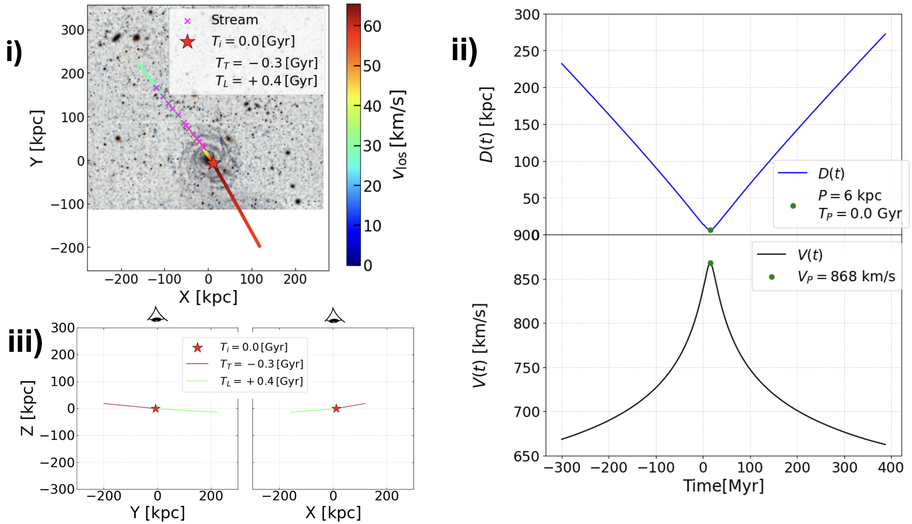
Figure 8: Scenario III-a: M1B+sB. Panel i) An example of an orbit integrated over $[-0.3,0.4]$ Gyr show not only a possible association of the sB as the leading component shown by magenta crosses with M1B represented by a red star as the progenitor. It is superimposed on the optical image of Malin 1 and its surroundings (Galaz et al., 2015). The color-bar illustrates LoS velocities along the orbit, having a maximum difference of $\Delta V_{\text{LoS}}\approx 60$ km/s. Legend shows stellar stream mark, the time for the progenitor (M1B), denoted (Ti), and the Trailing ($T_{T}$) and Leading ($T_{L}$) times with a common dot for both showing the colour or velocity of M1B at that specific moment of the orbit. The NFW profile was employed for this solution. Panel ii) Distance vs time, and a magnitude velocity vs time with $|V|\approx 868$ km/s. In this orbit, the pericenter passage of M1B occurred approximately $0.01$ Gyr. Panel iii) X-Z and Y-Z orbital planes. The best orbit has $z\sim-33$ kpc, $v_{t}\sim 998$ km/s, PA$\sim 36^{\circ}$, $R_{\text{peri}}\sim 35$ kpc, $R_{\text{apo}}\sim 9649$ kpc, and $\epsilon\sim 0.88$. The observer would be located at the top of these subpanel, at postitive Z and X, Y = (0, 0) kpc is the Malin 1 center. Legend shows the time for the progenitor, $T_{i}=0.0$ Gyr (present), and the Trailing, in purple colour, ($T_{T}=-0.3$ Gyr) and the Leading, in light green colour, ($T_{L}=0.4$ Gyr).

• Scenario III-b: M1B + sB + sA.
  This situation seeks M1B as the progenitor of sB and sA simultaneously, that is, as the leading and trailing streams with M1B at the core as the main progenitor. The pericentric passage is $32$ kpc with a velocity of $\sim 706$ km/s which happened 20. Myr ago. However, it was not possible to find a fitting orbit that connects both streams. Moreover, only an unbound orbit was the best solution. It is shown in panel ii) Fig. 13.

• Scenario IV-a: M1A + sA.
  Within the Malin 1 environment plot from (Galaz et al., 2015), Fig. 9 illustrates a best-fitted orbit that has been overemphasised. Three panels are used to describe this orbit. Panel i) An orbit simulation covering the time span $[-1.7,0.4]$ Gyr captures the visual aspects of Malin 1, identifying the possible trajectory for M1A (represented as a red star) along with a leading and trailing stellar stream (indicated by magenta crosses) as pointed out by (Niederste-Ostholt et al., 2012). The colour bar indicates LoS velocities, which can reach $\Delta V_{\text{LoS}}\approx 700$ km/s. Panel ii) A graph plotting the distance against time demonstrates the satellite’s orbit, highlighting a pericenter around $\sim 16$ kpc with a velocity magnitude of approximately $|V|\sim 488$ km/s at $\sim 1.3$ Gyr ago in the first passage. Panel iii) The orbit is shown in both the X-Z and Y-Z planes. In the accompanying corner plots (not shown here), the best fit parameters are $z\sim-138$ kpc, $v_{t}\sim 312$ km/s, PA$\sim 240^{\circ}$. The orbit properties include a periapsis of about $R_{\text{peri}}\sim 112$ kpc, an apoapsis of $R_{\text{apo}}\sim 246$ kpc and an ellipticity $\epsilon\sim 0.08$, which illustrates the eccentricity and scale of the orbit.

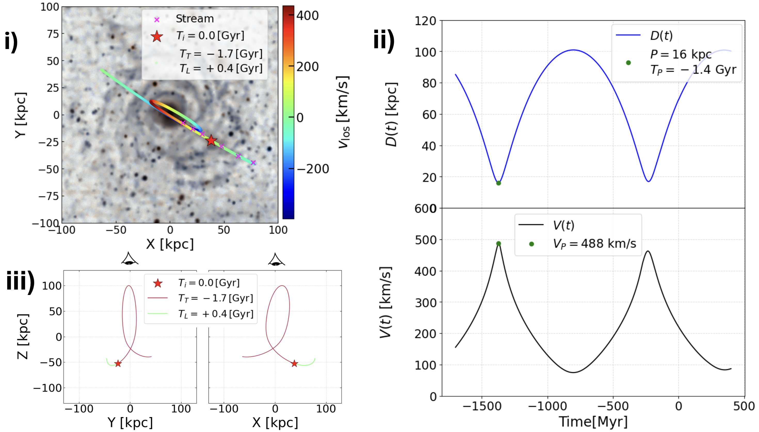
Figure 9: Scenario IV-a: M1A + sA. Panel i) A possible orbit integrated $[-1.7,0.4]$ Gyr over the optical image of Malin 1 and its environment (Galaz et al., 2015), revealing possible paths of M1A (red star) and a leading and trailing stellar stream arms (magenta crosses). The color bar represents LoS velocities reaching $\Delta V_{\text{LoS}}\approx 700$ km/s. This could be that both components of sA shows the trailing and leading stream components with M1A as the progenitor. Legend shows stellar stream mark, the time for the progenitor (M1A), denoted (Ti), and the Trailing ($T_{T}$) and Leading ($T_{L}$) times with a common dot for both showing the colour or velocity of M1C at that specific moment of the orbit. The isothermal profile was employed for the dark matter. Panel ii) The distance versus time graph illustrates the satellite’s orbital path, showing a pericenter near $\sim 16$ kpc with a velocity magnitude around $|V|\sim 488$ km/s, at $\sim 1.4$ Gyr ago in their first passage. Panel iii) X-Z and Y-Z orbital planes. The best orbit has $z\sim-138$ kpc, $v_{t}\sim 312$ km/s, PA$\sim 240^{\circ}$, $R_{\text{peri}}\sim 112$ kpc, an apoapsis at $R_{\text{apo}}\sim 246$ kpc, and an ellipticity $\epsilon\sim 0.08$. The observer would be located at the top of these subpanels, at postitive Z and X, Y = (0, 0) kpc is the Malin 1 center. Legend shows the time for the progenitor, $T_{i}=0.0$ Gyr (present), and the Trailing, in purple colour, ($T_{T}=-1.7$ Gyr) and the Leading, in light green colour, ($T_{L}=0.4$ Gyr).

• Scenario IV-b: M1A + sA + sB.
  In this scenario, M1A is identified as the origin of both sB and sA, acting as the foundational structure for the leading and trailing streams, with M1A located in the centre as the principal progenitor. However, an orbit linking the two streams could not be determined. The pericentric passage is $132$ kpc with a velocity of $\sim 553$ km/s which happened $1.1$ Gyr ago. However, it was not possible to find a fitting orbit that connects both streams. Moreover, only an unbound orbit was the best solution. It is shown in panel iii) Fig. 13.

• Scenario V-a: sA.
  The hypothesis is that the progenitor of sA has been completely tidally disrupted by the strong potential gravitational forces of Malin 1, leaving only sA as the remnant (Deason et al., 2023; Panithanpaisal et al., 2021). To investigate this, orbital computations were performed using leading and trailing integration. In Fig. 10, three panels are shown. Panel i) An integrated orbit over the time span $[-7.5,0.3]$ Gyr is showcased overlaying the optical image of Malin 1 (Galaz et al., 2015). This demonstrates the possible disintegration of the progenitor of sA (indicated by magenta crosses), with the last likely association point in sA marked by a red star. The colour bar indicates LoS velocities up to $\Delta V_{\text{LoS}}\sim 800$ km/s. Panel ii) The distance versus time graph reflects the dynamics of the satellite’s orbit, showing the minimum distance (pericenter) at $\sim 4.7$ kpc and a velocity magnitude of $D\sim 741$ km/s, at $\sim 4.7$ Gyr ago. Panel iii) Orbit views include X-Z and Y-Z planes. The best orbit has $z\sim-5.4$ kpc, $v_{t}\sim 590$ km/s, PA$\sim 240^{\circ}$, with orbital flat sample parameters of $R_{\text{peri}}\sim 13$ kpc, $R_{\text{apo}}\sim 250$ kpc and $\epsilon\sim 0.57$. The extremely small pericentres reveal that complete tidal disruption would be possible. It is interesting to note that M1A is in the debris of sA.

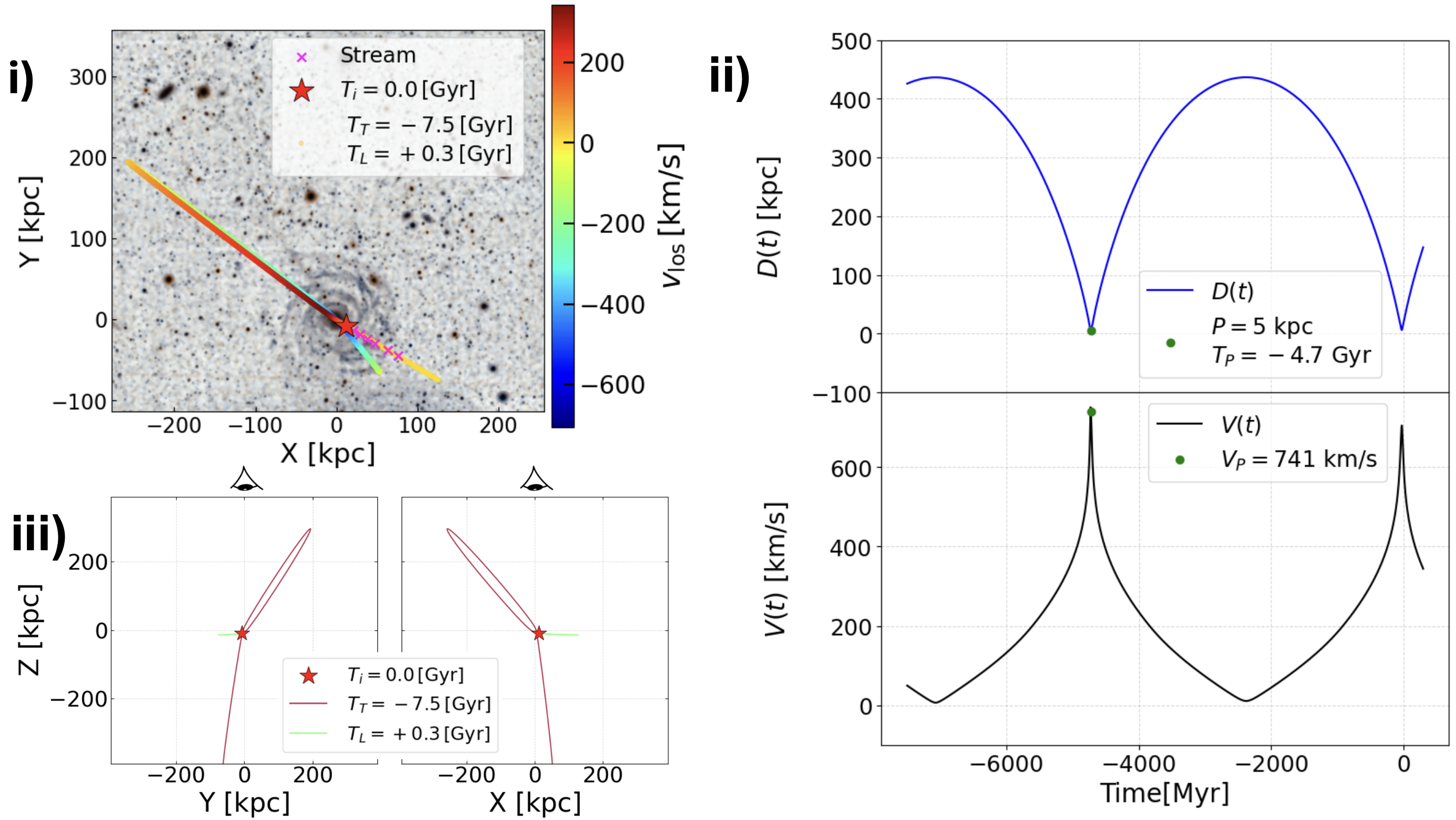
Figure 10: Scenario V-a: sA. The progenitor of sA has been completely tidally disrupted by the strong potential gravitational of Malin 1, leaving only sA as the remnant (Deason et al., 2023; Panithanpaisal et al., 2021). Panel i) A possible orbit spanning $[-7.5,0.5]$ Gyr maps the visual features of Malin 1, revealing possible path of a destroyed progenitor (red star) and a leading stellar stream sA (magenta crosses). The destroyed progenitor three dimensional position has been choose with the same M1B, $x$ and $y$ position, but $z=0.1$ kpc (diferent of $z=-43$ kpc found in scenario IIIa). The color bar represents LoS velocities reaching $\Delta V_{\text{LoS}}\approx 700$ km/s. In this destroyed situation sA could shows debris of the destroyed progenitor. Legend shows stellar stream mark, the time for the destroyed progenitor, denoted (Ti), and the Trailing ($T_{T}$) and Leading ($T_{L}$) times with a common dot for both showing the colour or velocity of the progenitor at that specific moment of the orbit. The isothermal profile was employed for the dark matter. Panel ii) The distance versus time graph illustrates the satellite’s orbital path, showing a pericenter near $\sim 4.7$ kpc with a velocity magnitude around $|V|\sim 741$ km/s, at $\sim 4.7$ Gyr ago. Panel iii) The orbit is depicted in the X-Z and Y-Z planes. The best-fit parameters are $z\sim-5.41$ kpc, $v_{t}\sim 590$ km/s, PA$\sim 240^{\circ}$, with the orbit’s characteristics including a periapsis at about $R_{\text{peri}}\sim 13$ kpc, an apoapsis at $R_{\text{apo}}\sim 250$ kpc, and an ellipticity $\epsilon\sim 0.57$. The observer would be located at the top of these subpanel, at postitive Z and X, Y = (0, 0) kpc is the Malin 1 center. Notoriusly, M1A belongs to sA. Legend shows the time for the progenitor, $T_{i}=0.0$ Gyr (present), and the Trailing, in purple colour, ($T_{T}=-7.5$ Gyr) and the Leading, in light green colour, ($T_{L}=0.3$ Gyr).

• Scenario V-b: sB.
  In this final scenario again, the possibility of a destruction event is examined. The hypothesis is that the progenitor sB has been completely tidally disrupted, leaving only sB as the remnant (Deason et al., 2023; Panithanpaisal et al., 2021). To investigate this, orbital computations were performed using leading and trailing integration. In Fig. 11, three panels are shown. Panel i) An integrated orbit over the time span $[-0.3,0.4]$ Gyr is showcased overlaying the optical image of the Malin 1 system (Galaz et al., 2015). This demonstrates the disintegration of the progenitor of sB (indicated by magenta crosses), with the last likely association with sB marked by a red star. The colour bar indicates LoS velocities up to $\Delta V_{\text{LoS}}\sim 175$ km/s. Panel ii) The distance versus time graph reflects the dynamics of the satellite’s orbit, showing the minimum distance (pericenter) at $\sim 14.06$ kpc and a velocity magnitude of $D\sim 938$ km/s happened $35$ Myr ago. Panel iii) Orbit views include X-Z and Y-Z planes. For the corner plots (not displayed), the top fitting parameters at the 50/100 percentile are $z\sim-7$ kpc, $v_{t}\sim 710$ km/s, PA$\sim 37^{\circ}$, with the orbital flat sample parameters being $R_{\text{peri}}\sim 10$ kpc, $R_{\text{apo}}\sim 3046$ kpc and $\epsilon\sim 0.88$. Interestingly, sB points to eM1.

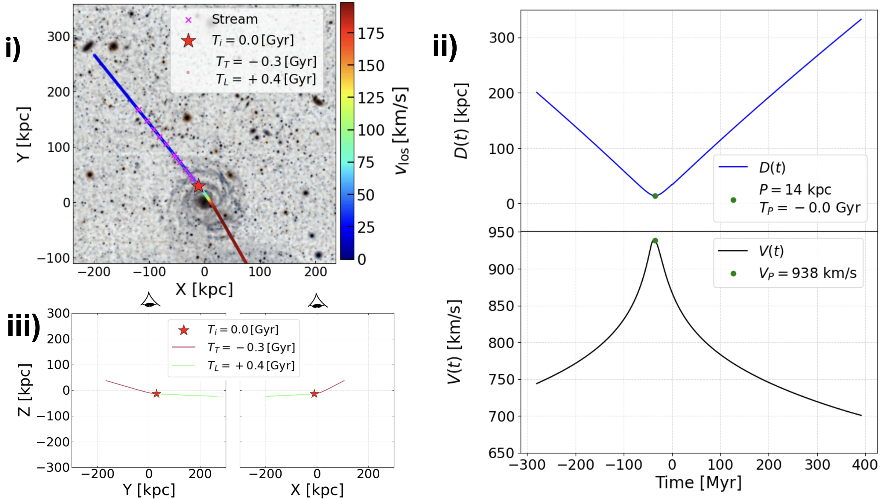
Figure 11: Scenario V-b: sB. The progenitor of sB has been completely tidally disrupted, leaving only sB as the remnant (Deason et al., 2023; Panithanpaisal et al., 2021). Panel i) An possible orbit over the time span $[-0.3,0.4]$ Gyr is showcased overlaying the optical image of Malin 1 and its vicinity (Galaz et al., 2015). This demonstrates the disintegration of the progenitor (indicated by magenta crosses). The destroyed progenitor three dimensional position has been choose with the same first sB point $x$ and $y$ position, and $z=Rtani=-24$ kpc. The colour bar indicates LoS velocities up to $\Delta V_{\text{LoS}}\sim 175$ km/s. In this new destroyed situation sA could it be debris of thr destroyed progenitor. Legend shows stellar stream mark, the time for the destroyed progenitor, denoted ($T_{i}$), and the Trailing ($T_{T}$) and Leading ($T_{L}$) times with a common dot for both showing the colour or velocity of the progenitor at that specific moment of the orbit. The isothermal profile was employed for the dark matter. Panel ii) The distance versus time graph reflects the dynamics of the satellite’s orbit, showing the minimum distance (pericenter) at $D\sim 14$ kpc and a velocity magnitude of $\sim 938$ km/s. Panel iii) Orbit views include X-Z and Y-Z planes. Panel iii) X-Z and Y-Z orbital planes. The best fitting parameters are $z\sim-7$ kpc, $v_{t}\sim 710$ km/s, PA$\sim 37^{\circ}$. The model with the maximum likelihood has orbital parameters $R_{\text{peri}}\sim 10$ kpc, $R_{\text{apo}}\sim 3046$ kpc, and $\epsilon\sim 0.88$. The observer would be located at the top of these subpanel, at postitive Z and X, Y = (0, 0) kpc is the Malin 1 center. Legend shows the time for the progenitor, $T_{i}=0.0$ Gyr (present), and the Trailing, in purple colour, ($T_{T}=-0.3$ Gyr) and the Leading, in light green colour, ($T_{L}=0.4$ Gyr). It is notorious that sB points to eM1.

4.3 Physical parameters

In addition, the determination of key physical parameters, such as the total length covered for the orbital solutions in Scenario I-a-radial and I-a-polar between the pericenter and the satellite eM1. The specific angular momentum for Malin 1 ($j_{*}$) (Di Teodoro et al., 2023), and the ratio $j_{*}/j_{200}$, where $j_{200}$ is $j_{*}$ within the virial ratio (Pérez-Montaño et al., 2022). The stellar mass-to-light ratio for each dark mater profile. The total luminosity in the R band (following (Mo, 2010)). The total stellar mass using the pseudo-isothermal profile and the virial radius and virial mass, provides essential constraints on the mass distribution and dynamics of the system. This result can be seen in Table 5.

Our results suggest that Malin 1 adheres to the Fall relation, which supports the notion that giant low surface brightness galaxies (gLSBGs) might evolve differently from high-surface brightness spirals, aligning instead with other gLSBGs. Furthermore, Malin 1 possesses a greater specific angular momentum compared to the Milky Way, largely due to its vast size (refer to Section 5).

Table 5: Physical results from the Models. Specific Angular Momentum ($j_{*}$), and $j_{200}$ is $j_{*}$ at virial radius (Pérez-Montaño et al., 2022). Mass to Light ratio using the NFW model and the Isothermal one. Total luminosity in the $R$ band. Stellar mass using the NFW model. Stellar mass using the Isothermal model. Virial Mass. Dynamical masses. Length of the orbital solution between the pericenter and the satellite eM1 for the radial and polar solutions in scenario I-a.

Parameter	Value
$j_{*}/j_{200}$	$0.21$ a
$({M/L_{\rm R}})_{\rm NFW}$	$\mathrm{3.2\pm 0.5}\,\mathrm{M_{\odot}/L_{\odot}}$ b
$(M/L_{\rm R})_{\rm Iso}$	$\mathrm{3.4\pm 0.5}\,\mathrm{M_{\odot}/L_{\odot}}$ b
$L_{\rm R,Total}$	$1.9\pm 0.6\times 10^{11}\,\mathrm{L_{\odot}}$ c
$M_{\rm Stellar,\,NFW}$	$2.3\pm 1\times 10^{11}\,\mathrm{M_{\odot}}$ d
$M_{\rm Stellar,\,Iso}$	$4.8\pm 1\times 10^{11}\,\mathrm{M_{\odot}}$ d
$R_{Virial-NFW}$	$247$ kpc e
$R_{Virial-Iso}$	$323$ kpc e
$M_{Dyn-NFW}$	$1.7\times 10^{12}\,\mathrm{M_{\odot}}$ f
$M_{Dyn-Iso}$	$3.8\times 10^{12}\,\mathrm{M_{\odot}}$ f
$l_{Malin1-radial}$	$480\;\text{kpc}$ g
$l_{Malin1-polar}$	$738\;\text{kpc}$ g

^a $j_{*}/j_{200}$ ratio for Malin 1, reported in Pérez-Montaño et al. (see Fig. 7 in 2022). ^b $M/L$ represent the stellar mass-to-light ratio, obtained in the R-band surface brightness profile (Lelli et al., 2010), using NFW and pseudo-Isothermal dark halo profiles. The resuls obtained are in concordance with Lelli et al. (2010). ^c Total luminosity obtained in the R-band. ^d Total stellar mass obtained using the Isothermal profile, half the value reported by Saha et al. (2021) ^e Virial radius obtained using NFW and Isothermal profiles as in Mo (2010). ^f Total mass inside the Virial radio for NFW and Isothermal profiles as in Mo (2010). ^g The radial length is less than the polar one as it must be. The last describes a solution like the discovery by Martínez-Delgado et al. (2021).

5 Discussion

The Malin 1 system, which includes four satellites and two stellar streams, was analysed to identify possible historical interactions for each satellite and possible alignment with the streams. Various orbital scenarios linking Malin 1, the stellar streams and their satellites are depicted in Fig.5 $-$ Fig.11. It was observed that each satellite’s line-of-sight distance from Malin 1 varies based on the specific scenario considered, as elaborated further in the discussion. Our findings suggest that the streams may be trailing, leading, or both. Future kinematic measurements of the streams could provide insights into their orbital history.

The Malin 1 system exhibits a dynamical configuration, characterised by two significant possible streams, sA and sB, as well as at least four satellite galaxies, M1A, M1B, M1C and eM1. Of these, M1B and eM1 have been reported as satellites by Reshetnikov et al. (2010), M1B is close to the centre, while eM1 is at 350 kpc in the northeast. M1A and M1B are also reported as compact ellipticals (cE) (Saburova & Cherepashchuk, 2021), likely resulting from the tidal stripping of massive progenitors (Saburova et al., 2023). Similar processes were observed in other galaxies, such as UGC 1382 (Saburova & Cherepashchuk, 2021). M1C could be an UDG (Ji et al., 2021). However, some authors claim M1C as a young star-forming region of $\sim 3$ arcsec of apparent radius, consistent with point 41 of Fig. 3 of Junais et al. (2024), showing H$\alpha$ emission (Junais et al., 2024, and private communication). If the last H$\alpha$ emission region is confirmed, then Scenario II-a and II-b could be rejected as the search for the stream progenitors.

Using a NFW dark mater model and a pseudoisothermal model, it was observed that for our solutions, bound orbits were achieved with most likelihood with the isothermal profile. This outcome arises because the isothermal profile predicts a larger mass distribution at greater distances, offering a better fit to the experimental data, as illustrated in the bottom panel in Fig. 2.

Other studies show a possible connection between the cE and their parent spiral galaxy, such as M32 and the Andromeda galaxy stream (Ibata et al., 2004; Fardal et al., 2006). This evidence supports the hypothesis that the cEs, M1A, M1B, and likely M1C could also be identified as progenitors of streams A and B. Similar conclusions have been derived for other galaxies. For example, a giant galactic tail reported to have a value greater than $350$ kpc and called ”Kite” (Zaritsky et al., 2023) or the giant stream of $\sim 500$ kpc generated by a dwarf galaxy in the Coma cluster (Román et al., 2023) supports the existence of large streams, for example, stream B, which connects linearly in projection, eM1, with Malin 1. If the off-centre detected in eM1 (Fig. 1 - point 4) indicates ongoing star formation, it could suggest that gas inflows or disturbances have initiated star formation away from the centre. This could be due to a possible interaction or merging event, where tidal forces have displaced the galaxy’s core. Such phenomena are often observed in galaxies that undergo gravitational interactions, resulting in an off-centre core or an asymmetric disk (Mao et al., 2021).

The connection of our orbital solutions with possible progenitors and streams aligns well with survey observations, such as those noted by Zaritsky et al. (2023); Román et al. (2023).

As demonstrated by Zhu et al. (2018), the simulation of the formation of a Malin 1-like galaxy involves the stimulated accretion due to cooling of a hot halo gas, caused by the merger of two satellite galaxies (intruders), leading to the creation of a large galactic disk at $z=0$.

Martínez-Delgado et al. (2021) suggest that examining the formation of tidal streams could provide insight into the timing of major merger events. In the case of Malin 1, some or all satellites could contribute via wet mergers with the size of the main galaxy. The pericenters pass at $\sim-1.3$ Gyr, for scenario I-a-radial (eM1+sB-radial), $\sim-1.3$ Gyr, for scenario I-a-polar (eM1+sB-polar), the trailing pericenter passage occurred approximately $-0.1$ Gyr ago, whereas it was about $2.3$ Gyr for the leading arm in scenario II-b (M1C+sA+sB), $-4.2$ Gyr, for scenario III-a (M1B+sB), $-1.3$ Gyr, for scenario IV-a (MA1+sA), $-4.7$ Gyr, for scenario V-a (sA only) and $-0.04$ Gyr, for scenario V-b (sB only). It could be proposed that the evolution of Malin 1 likely involved a significant wet major merger approximately $1.3$ Gyr ago, influenced by the eM1 passage. In addition, M1B contributes $4.3$ Gyr ago, M1A $-1.3$ Gyr ago, and M1C with the leading stream $2.3$ Gyr and $-0.1$ Gyr for the trailing component (Martínez-Delgado et al., 2021).

In Scenario I-a-r: eM1 + sB, radial orbit, seeing in Fig. 5, the pericenter passage of eM1 occurred $\sim 1.3$ Gyr ago (z $\approx$ 0.1). In addition, eM1 shows evidence of emission lines of H$\alpha$, H$\beta$, and OII, so it is a star-forming disk galaxy (SDSS SkyServer, 2024; Lintott et al., 2011). The movement of eM1 started in our analysis $\sim 13$ Gyr ago ($z\approx 6.8$), and the pericenter passage $z\approx 6.8$ so their evolution would help increase the gas in Malin 1 placing eM1 as another candidate progenitor of sB.

Scenario I-a-p: eM1 + sB, polar orbit. This approach could help model stellar streams in circular orbits, such as the one of the sombrero galaxy (Martínez-Delgado et al., 2021), the satellite galaxy could be eM1 in a polar orbit, as appreciated in panel iii) Fig. 6.

An interesting situation is Scenario I-b: eM1 + sA + sB, which attempts to connect both streams; however, it was not possible to find a bound orbit. The best unbound is shown in panel i) in Fig. 13. The same unbound situation repeats in Scenario III-b, and Scenario IV-b, as shown in panels ii) and iii) in Fig. 13 respectively.

In Scenario II-a, M1C + sB presents strong support for the hypothesis that M1C, potentially an Ultra Diffuse Galaxy (UDG) (Ji et al., 2021), serves as proof that sB has leading and trailing sections, in line with what Niederste-Ostholt et al. (2012) proposed by identifying M1C as the progenitor. This scenario is illustrated in panel iv) of Fig. 13. In contrast, adding sA as a stream linked to sB with M1C as the source for both streams, that is, scenario II-b: M1C + sA + sB, offers a compelling solution that not only unites both streams, but also reenacts Scenario II-a. This solution is depicted in Fig. 7. It is notorious how all orbits show us the radial behaviour and intriguing connection of leading and trailing components of the large stream.

Scenario III-a examines M1B + sB, involving a pericenter passage $\sim 0.01$ Gyr, as illustrated in Fig. 8. This scenario is also recognised by Zhu et al. (2018) as a potential intruder galaxy due to the ancient interaction that possibly contributes to stimulated accretion. Currently, stream B functions as the leading arm with M1B as its progenitor, and the trailing segment also exhibits radial behaviour.

M1A + sA, or scenario IV-a, is a innovative configuration, M1A being the other cE as the core or leading and trailing components of sA. In this arrangement, the pericenter is $\sim 16.1\pm 1.2$ kpc, which confirms that M1A is another possible cause of triggering regions of star formation in the central part of the galaxy as reported by (Lelli et al., 2010).

In the last scenario (IV-a) it was also interesting to find polar orbits (not shown), so sA could be a tidal tail perpendicular to the orbit.

Finally, scenarios V-a: sA and V-b: sB are novel configurations because they explore a possible tidal disruption of the progenitor (Deason et al., 2023; Panithanpaisal et al., 2021). For both, radial orbits (low circularity) were founded, which could mean that the streams formed very recently (Panithanpaisal et al., 2021). Scenario V-a shows us a total disconnect from sB, which is interesting per se as an independent event. Moreover, it is connected with M1A which reinforces the possibility that sA is strong evidence of some past interaction between M1 and a destroyed progenitor that also connects M1A. Scenario V-b is also remarkable because it does not connect sB with sA and plays in that way an equivalent situation where the possible progenitor was destroyed and we can see only debris from it in sB. Furthermore, M1C could be a region of star formation activated by this passage, as a discovery of Junais et al. (2024).

Our orbital analysis presents favourable results for all satellites M1B, M1A, M1C, and eM1. Moreover, for destroyed ones, as the last two scenarios analysed (V-a and V-b).

In the past, if the satellites M1A, M1B, and M1C contained more gas, they could have triggered stimulated accretion around approximately $\sim-4.7$, $\sim 4.2$, and $\sim-2.3$ billion years ago, respectively, which could have contributed to the considerable size of Malin 1 (Zhu et al., 2018).

Another compelling point supporting the possibility that eM1 aligns with Malin 1 is that aligned mergers in relatively isolated environments may facilitate the development of expansive discs, similar to Malin 1’s galaxy, with no ongoing mergers currently (Zhu et al., 2023).

Pérez-Montaño et al. (2022) have further observed that LSBGs exhibit a greater connection between their specific angular momentum and dark matter compared to HSBGs. Our result, reported in Table 5, is consistent with that study. The ratio of specific angular momentum to the angular momentum in the virial radius, denoted as $j_{*}/j_{200}$, places Malin 1 in line with the Fall relation suggested by Fall (1983). This result agrees with the findings illustrated in Pérez-Montaño et al. (2022, Fig. 7,). This evidence highlights Malin 1 as a galaxy that exhibits significant specific angular momentum (Di Teodoro et al., 2023; Pérez-Montaño et al., 2022). The specific angular momentum found still has a larger one than the Milky Way, primarily because of its enormous size. This suggests that Malin 1 is a key system for understanding the formation and angular-momentum evolution of these gLSBG. (Aditya et al., 2023, private communications with Aditya.). Furthermore, the substantial specific angular momentum of Malin 1 could indicate past interactions that resulted in the accretion of some satellites by the giant LSB galaxy (Zhu et al., 2018).

The warp and cavity observed in Malin 1 could result from gravitational interactions with nearby and distant satellites. For example, orbital solutions from Scenarios II-b (M1C+sA+sB) and III-a (M1B+sB) show trajectories near the cavity, suggesting that gravitational forces combined with Malin 1’s rotation influence its development. The last pericenter passage of M1C (scenario II-b) was $\sim 0.1$ Gyr ago, which is consistent with some warped models (Binney, 2024). Also, a flyby of eM1 with pericenter pass $1.3$ Gyr ago may help explain the HI disk warp. Interactions between galaxies are the main responsible for warped disk (Kalberla & Kerp, 2009; Kim et al., 2014)

One of the constraints of our study comes from the lack of extensive data. This limitation is especially significant s the intricate spatial configuration of the streams. It also applies to their velocity patterns at various locations. Future research should aim to investigate other elements of the streams. These may include components that might have been overlooked. Conducting a specialised kinematic survey of the Malin 1 system entails assessing the velocities of various constituents within and surrounding this giant Low-Surface Brightness (LSB) galaxy, such as its stellar and gaseous components and satellite galaxies.

N-body simulations should serve as the next stage in our investigation to predict specific scenarios. This technique will clarify the connections between streams and the initiation of satellites. Furthermore, it will validate our orbital solutions within the Malin 1 system.

An additional significant approach for future research might involve investigating a three-body or three-galaxy system, designating the heaviest galaxies as M1 and eM1, while the third, smaller one might be chosen from among M1B, M1A, or M1C, to further elucidate the presence of giant stellar streams (Zaritsky et al., 2023).

6 Summary and future work

We explored the orbital dynamics of the satellite galaxies surrounding Malin 1 and their connection to stellar streams. By utilising HI and R-band data, we developed gravitational potential models that include stellar, gaseous, and dark matter elements. Through Monte Carlo Markov Chain (MCMC) simulations, we analysed their trajectories within both the Navarro-Frenk-White and isothermal-halo frameworks. Our results emphasise the influence of historical interactions on the development of the Malin 1 extended disk and the increase in its gas abundance. The core results of this research are outlined below.

The Malin 1 system revealed two giant stellar stream candidates, sA and sB, and four satellite galaxy candidates: M1A, M1B, M1C, and eM1.

Orbital simulations emphasised the crucial importance of the dark matter halo, revealing that massive halos provide improved models for the gravitationally bound paths of satellites. Our models suggest orbital solutions that may link M1A and M1B, classified as compact ellipticals (cE), to the stellar streams. This possible link aligns with the formation theories for cE galaxies that undergo significant tidal stripping, similar to the interaction between M31 and M32 (Ibata et al., 2004).

The nature of M1C is still not clearly defined. Its H$\alpha$ emission and structure imply that it may be an H$\alpha$ blob, as suggested by Ji et al. (2021), within the scope of ultradiffuse galaxies (UDG). However, evidence of stellar emissions also suggests that M1C might be either a substantial nuclear star cluster (Antonini, 2013) or a blob forming stars (Junais et al., 2024, private communication). More studies are essential to determine its actual identity.

M1C is in the centre of stream sB. We identified orbits that can link M1C with the leading and trailing components of the stream, which exhibit approximate symmetry (Niederste-Ostholt et al., 2012). Studies indicate that tidal stripping could be responsible for the creation of cE galaxies such as M1A and M1B (Chilingarian et al., 2015). In Scenario IV-a (M1A+sA), orbital configurations unite the two cE galaxies, while Scenario II-b (M1C+sA+sB) associates the streams with the cE galaxies, identifying the core of sB as M1C.

Satellite destruction creates debris streams, as shown in scenarios V-a and V-b, highlighting gravitational potential interactions. In particular, in scenario V-b, sB is directed toward the eM1 position (Deason et al., 2023; Panithanpaisal et al., 2021). Moreover, small pericentres would lead to strong tidal stripping, for example, $4.7$ kpc for scenario V-a (sA only) or $14.0$ kpc for scenario V-b (sB only). Satellites in close pericentric encounters have been shown to enhance star formation (Saha et al., 2021), as is similarly observed in scenarios III-a (M1B + sB) and IV-a (M1A + sA) interactions.

The most probable scenario for the formation of the two streams could be Scenario II-b (M1C + sA + sB). To explain sB as a radial connection between eM1 and M1, scenario I-a radial orbit (eM1 + sB - radial) and a polar orbit with eM1 as progenitor and sB not in the galactic plane, scenario I-a polar (eM1 + sB - polar). To explain sB as the leading component of M1B, scenario III-a (M1B + sB) and to study the leading and trailing components with M1A as progenitor, scenario IV-a (M1A + sA). For the destruction process involves scenarios V-a (sA) and V-b (sB).

The ratio of the specific angular momentum to that in the virial radius, $j_{*}/j_{200}$, aligns Malin 1 in agreement with the Fall relation as proposed by Fall (1983). This value is consistent with the results presented in Pérez-Montaño et al. (2022, Fig. 7). This observation underscores Malin 1 as a galaxy with a high specific angular momentum (Di Teodoro et al., 2023; Pérez-Montaño et al., 2022) and could play a crucial role in future comparative studies with other gLSBGs.

Future photometric and spectroscopic studies may reveal a wide parameter space information, which will help to improve the connection between observations and semi-analytical models.

More detailed photometric studies are essential to uncover the complete range and complex details of the stellar streams surrounding Malin 1. These studies have the potential to identify previously unnoticed streams and provide insight into their orientation, composition, and relationships with satellite encounters. This information would greatly improve our comprehension of the system’s dynamic history and its significance in models of galaxy formation. For example, upcoming MUSE data for the entire Malin 1 disk (Galaz et al. in preparation) will help refine our models by incorporating information on HII regions and metallicities throughout the disc, whereas JWST data will soon investigate the Kennicutt relation (Berg et al., 2024).

N-body simulations are set to predict particular scenarios within the Malin 1 system and will investigate mergers occurring at high redshift and the tidal disturbance of stellar streams by satellites. These efforts aim to elucidate the mechanisms behind stream-satellite interactions and to examine the semi-analytical solutions applied in our research. These simulations are set to investigate the development and stability of the warp in the disk of Malin 1, possibly caused by internal dynamics (Saha et al., 2010) or interactions with its satellites (Bonaca et al., 2021). Understanding the origin of the streams is vital to uncovering the impact of satellites and tidal forces on the distinctive shape of the galaxy system. Furthermore, this work seeks to shed light on the mechanics of stream-satellite interactions and to assess the semianalytical models used in our study.

Given these considerations, it is essential to rapidly examine new satellite candidates, such as the three galaxies with roughly the same redshift situated about 1 Mpc from Malin 1 (Bustos et al. in prep.).

Taken together, this research efforts offer an essential comparative framework for understanding the development of gLSBG systems like Malin 1. This framework includes a detailed analysis of critical components such as optimal orbital solutions, satellite angular momentum, and stellar stream dynamics, as investigated in studies by (Zhu et al., 2018; Mapelli et al., 2008; Di Teodoro et al., 2023). These studies emphasise the significance of satellite interactions, mergers, and streams as indicators of past interactions, extended disks, and gas enrichment within these galaxies, aligning with the current models of galaxy formation.

Appendix A Stream Points

Table 6 presents the Stream Points, i.e., Points obtained as prior information for the Monte Carlo Markov chain mcmc-emcee method (Foreman-Mackey et al. 2012) using visual observation on the Fig. 1 (Galaz et al., 2015).

Table 6: Stream Points sA (7 points) and sB (13 points). They are observational Points used as inputs in the Markov chain Monte Carlo technique mcmc-emcee (Foreman-Mackey et al., 2012). The four (4) satellites positions are included. The statistical accuracy of each coordinate $x$ and $y$ was enhanced by using the projected angular scale and the median seeing of $0.8$ arcsec (Galaz et al., 2015), given a confidence level of $\pm 1$ kpc. For the radial distance a propagation error was used.

Object	$\alpha$ (2000)	$\delta$ (2000)	x [kpc]	y [kpc]	r [kpc]
Malin 1	12:36:59.36	14:19:49.4	$0\pm 1$	$0\pm 1$	$0$
sA1: M1B	12:36:58.89	14:19:43.9	$12\pm 1$	$-8\pm 1$	$14\pm 1$
sA2	12:36:58.42	14:19:39.4	$21\pm 1$	$-13\pm 1$	$25\pm 1$
sA3	12:36:58.03	14:19:36.1	$30\pm 1$	$-18\pm 1$	$35\pm 1$
sA4: M1A	12:36:57.62	14:19:32.9	$38\pm 1$	$-24\pm 1$	$45\pm 1$
sA5	12:36:57.12	14:19:28.2	$47\pm 1$	$-29\pm 1$	$56\pm 1$
sA6	12:36:56.78	14:19:26.8	$63\pm 1$	$-38\pm 1$	$74\pm 1$
sA7	12:36:56.47	14:19:24.9	$77\pm 1$	$-44\pm 1$	$89\pm 1$
sB1	12:36:59.98	14:20:07.1	$-11\pm 1$	$29\pm 1$	$31\pm 1$
sB2	12:37:00.02	14:20:12.1	$-13\pm 1$	$34\pm 1$	$37\pm 1$
sB3: M1C	12:37:00.36	14:20:16.8	$-22\pm 1$	$42\pm 1$	$47\pm 1$
sB4	12:37:00.65	14:20:22.6	$-27\pm 1$	$50\pm 1$	$57\pm 1$
sB5	12:37:01.03	14:20:27.6	$-34\pm 1$	$59\pm 1$	$69\pm 1$
sB6	12:37:01.34	14:20:34.4	$-45\pm 1$	$72\pm 1$	$85\pm 1$
sB7	12:37:01.68	14:20:41.3	$-52\pm 1$	$80\pm 1$	$95\pm 1$
sB8	12:37:01.70	14:20:41.6	$-55\pm 1$	$85\pm 1$	$102\pm 1$
sB9	12:37:02.69	14:20:56.4	$-69\pm 1$	$105\pm 1$	$125\pm 1$
sB10	12:37:03.22	14:21:02.9	$-81\pm 1$	$118\pm 1$	$144\pm 1$
sB11	12:37:03.55	14:21:12.2	$-92\pm 1$	$131\pm 1$	$160\pm 1$
sB12	12:37:04.10	14:21:24.8	$-103\pm 1$	$147\pm 1$	$180\pm 1$
sB13	12:37:04.85	14:21:37.8	$-119\pm 1$	$167\pm 1$	$205\pm 1$
eM1	12:37:08.92	14:22:53.3	$-211\pm 1$	$278\pm 1$	$349\pm 1$

Appendix B Best parameters Fit using Monte Carlo Markov Chain mcmc-emcee

Monte Carlo Markov chain mcmc-emcee (Foreman-Mackey et al., 2012; Hogg et al., 2010) to determine the best fitting parameters for the surface brightness profile and the rotational velocity is shown in Table 7.

mcmc-emcee (Foreman-Mackey et al., 2012; Hogg et al., 2010) corner plots that show the orbital parameters of maximum likelihood are shown in Table 8.

Table 7: Markov chain Monte Carlo mcmc-emcee (Foreman-Mackey et al., 2012; Hogg et al., 2010) to determine the best fitting parameters for the surface brightness profile and the rotation curve profile.

$Parameter$	$Value$
$a_{0}$	$(1.00\pm 0.05)\,\text{kpc}$
$b_{0}$	$0.0$ kpc
$a_{1}$	$(4.6\pm 0.3)\,\text{kpc}$
$b_{1}$	$0.0$ kpc
$z_{1}$	$0.3$ kpc
$a_{2}$	$(94^{+7}_{-6})\,\text{kpc}$
$b_{2}$	$0.0$ kpc
$z_{2}$	$0.3$ kpc
$a_{3}$	$93$ kpc
$b_{3}$	$0.0$ kpc
$z_{3}$	$0.0$ kpc
$L_{0}$	$1.25^{+0.06}_{-0.06}\times 10^{10}\,L_{\odot}$
$L_{1}$	$2.33^{+0.07}_{-0.07}\times 10^{10}\,L_{\odot}$
$L_{2}$	$7.1^{+0.6}_{-0.5}\times 10^{10}\,L_{\odot}$
$(M/L)_{NFW}$	$3.2^{+0.5}_{-0.5}\,(M/L)_{\odot}$
$(M/L)_{Isothermal}$	$3.4^{+0.5}_{-0.5}\,(M/L)_{\odot}$
$\rho_{0}$	$\sim 6^{+2}_{-3}\times 10^{6}\,M_{\odot}\,\text{pc}^{-3}$
$l_{s}$	$\sim 21^{+6}_{-3}\,\text{kpc}$

Table 8: Markov chain Monte Carlo mcmc-emcee (Foreman-Mackey et al., 2012; Hogg et al., 2010) corner plot distributioins showing the maximum likelihood orbital parameters for the bound orbits found.

Scenario	$z$ [kpc]	$v_{t}$ [km/s]	PA [deg]	$R_{\text{peri}}$ [kpc]	$R_{\text{apo}}$ [kpc]	Ellipticity
Ia	$-8$	$532$	$39$	$357$	$4775$	$0.47$
IIa	$1$	$472$	$217$	$28$	$378$	$0.50$
IIb	$-64$	$378$	$217$	$49$	$296$	$0.30$
IIIa	$-43$	$66$	$1$	$55$	$257$	$0.33$
IVa	$-138$	$311$	$0$	$112$	$246$	$0.08$
Va	$-5$	$590$	$0$	$13$	$250$	$0.57$
Vb	$-7$	$711$	$0$	$10$	$3046$	$0.88$

References

- Abazajian et al. (2009) Abazajian, K. N., Adelman-Mccarthy, J. K., Agüeros, M. A., et al. 2009, Astrophysical Journal, Supplement Series, 182, 543
- Aditya et al. (2023) Aditya, K., Banerjee, A., Kamphuis, P., et al. 2023, Monthly Notices of the Royal Astronomical Society, 526, 29
- Antonini (2013) Antonini, F. 2013, Astrophysical Journal, 763
- Bannikova (2018) Bannikova, E. Y. 2018, Monthly Notices of the Royal Astronomical Society, 476, 3269
- Barth (2007) Barth, A. J. 2007, A NORMAL STELLAR DISK IN THE GALAXY MALIN 1 1, Tech. rep.
- Bekki et al. (2001) Bekki, K., Couch, W. J., & Drinkwater, M. J. 2001, GALAXY THRESHING AND THE FORMATION OF ULTRACOMPACT DWARF GALAXIES, Tech. rep.
- Bell & De Jong (2001) Bell, E. F. & De Jong, R. S. 2001, STELLAR MASS-TO-LIGHT RATIOS AND THE TULLY-FISHER RELATION, Tech. rep.
- Berg et al. (2024) Berg, M., Galaz, G., Puzia, T., et al. 2024, 5394-Untangling the Nature of the Kennicutt Relation at the Low End: the Iconic Case of the Giant Low Surface Brightness Galaxy Malin 1, Tech. rep.
- Binney (2024) Binney, J. 2024
- Binney J. & Tremaine S. (2008) Binney J. & Tremaine S. 2008
- Blair et al. (2019) Blair, W. P., Long, K. S., Winkler, P. F., Lacey, C. K., & Williams, B. F. 2019, The Fireworks Galaxy, NGC 6946: Looking at the Fading Embers, Tech. rep.
- Blaña et al. (2020) Blaña, M., Burkert, A., Fellhauer, M., Schartmann, M., & Alig, C. 2020, Monthly Notices of the Royal Astronomical Society, 497, 3601
- Boissier et al. (2016) Boissier, S., Boselli, A., Ferrarese, L., et al. 2016, The properties of the Malin 1 galaxy giant disk: A panchromatic view from the NGVS and GUViCS surveys, Tech. rep.
- Bonaca et al. (2021) Bonaca, A., Naidu, R. P., Conroy, C., et al. 2021, The Astrophysical Journal Letters, 909, L26
- Bothun et al. (1987) Bothun, G. D., Lmpey, C. D., Malin, D. F., & Mould, J. R. 1987, DISCOVERY OF A HUGE LOW-SURFACE-BRIGHTNESS GALAXY: A PROTODISK GALAXY AT LOW REDSHIFT?, Tech. Rep. 1
- Bustos-Espinoza et al. (2023) Bustos-Espinoza, R. O. E., Blaña, M., Galaz, G., & Gil, S. 2023, in XVII Latin American Regional IAU Meeting, Uruguay, ed. C. Mateu (México: Revista Mexicana de Astronomía), 1–1
- Chilingarian et al. (2015) Chilingarian, I., Lau, R. M., Herter, T. L., et al. 2015, Science, 348, 413
- Cook et al. (2023) Cook, D. O., Mazzarella, J. M., Helou, G., et al. 2023, The Astrophysical Journal Supplement Series, 268, 14
- Das (2013) Das, M. 2013, Giant Low Surface Brightness Galaxies: Evolution in Isolation, Tech. rep.
- De Blok & Bosma (2002) De Blok, W. J. & Bosma, A. 2002, Astronomy and Astrophysics, 385, 816
- Deason & Belokurov (2024) Deason, A. J. & Belokurov, V. 2024, Galactic Archaeology with Gaia
- Deason et al. (2023) Deason, A. J., Koposov, S. E., Fattahi, A., & Grand, R. J. 2023, Monthly Notices of the Royal Astronomical Society, 520, 6091
- Dey et al. (2019) Dey, A., Schlegel, D. J., Lang, D., et al. 2019, The Astronomical Journal, 157, 168
- Di Teodoro et al. (2023) Di Teodoro, E. M., Posti, L., Fall, S. M., et al. 2023, Monthly Notices of the Royal Astronomical Society, 518, 6340
- Disney (1976) Disney. 1976
- Du et al. (2020) Du, W., Cheng, C., Zheng, Z., & Wu, H. 2020, The Astronomical Journal, 159, 138
- Fall (1983) Fall. 1983
- Fardal et al. (2006) Fardal, M. A., Babul, A., Geehan, J. J., & Guhathakurta, P. 2006, Monthly Notices of the Royal Astronomical Society, 366, 1012
- Fellhauer et al. (2006) Fellhauer, M., Evans, N. W., Belokurov, V., et al. 2006, Is Ursa Major II the Progenitor of the Orphan Stream?, Tech. rep.
- Foreman-Mackey et al. (2012) Foreman-Mackey, D., Hogg, D. W., Lang, D., & Goodman, J. 2012
- Freeman (1970) Freeman, K. C. 1970, ON THE DISKS OF SPIRAL AND SO GALAXIES, Tech. rep.
- Galaz et al. (2022) Galaz, G., Frayer, D. T., Blaña, M., et al. 2022, The Astrophysical Journal Letters, 940, L37
- Galaz et al. (2024) Galaz, G., González-López, J., Guzmán, V., et al. 2024
- Galaz et al. (2015) Galaz, G., Milovic, C., Suc, V., et al. 2015, The Astrophysical Journal, 815, L29
- Gerritsen & De Blok (1999) Gerritsen, J. P. E. & De Blok, W. J. G. 1999, Star formation and the interstellar medium in low surface brightness galaxies III. Why they are blue, thin and poor in molecular gas, Tech. rep.
- Hoffman et al. (1992) Hoffman, Y., Silk, J., & Wyse, R. F. G. 1992, THE FORMATION OF GIANT LOW SURFACE BRIGHTNESS GALAXIES, Tech. rep.
- Hogg et al. (2010) Hogg, D. W., Bovy, J., & Lang, D. 2010, Data analysis recipes: Fitting a model to data *, Tech. rep.
- Ibata et al. (2004) Ibata, R., Chapman, S., Ferguson, A. M., et al. 2004, Taking measure of the Andromeda halo: A kinematic analysis of the giant stream surrounding M31
- Impey & Bothun (1997) Impey, C. & Bothun, G. 1997, LOW SURFACE BRIGHTNESS GALAXIES, Tech. rep.
- Ji et al. (2021) Ji, X., Li, C., Yan, R., et al. 2021, Monthly Notices of the Royal Astronomical Society, 508, 3943
- Johnston et al. (2024) Johnston, E. J., Galaz, G., Blaña, M., et al. 2024, Astronomy and Astrophysics, 686
- Junais et al. (2024) Junais, Weilbacher, P. M., Epinat, B., et al. 2024, Astronomy and Astrophysics, 681
- Kalberla & Kerp (2009) Kalberla, P. M. & Kerp, J. 2009, Annual Review of Astronomy and Astrophysics, 47, 27
- Kazantzidis S. et al. (2003) Kazantzidis S., Satellites, T., Streams, . L. P. ., Prada, F., Martínez-Delgado, D., & Mahoney, T. 2003, Galaxies and Overmerging: What Does it Take to Destroy a Satellite Galaxy?, Tech. rep.
- Kim et al. (2014) Kim, J. H., Peirani, S., Kim, S., et al. 2014
- Kim et al. (2020) Kim, S., Jeong, H., Rey, S.-C., et al. 2020, The Astrophysical Journal, 903, 65
- Lelli et al. (2010) Lelli, F., Fraternali, F., & Sancisi, R. 2010
- Lintott et al. (2011) Lintott, C., Schawinski, K., Bamford, S., et al. 2011, Monthly Notices of the Royal Astronomical Society, 410, 166
- Long & Murali (1992) Long & Murali. 1992
- Maeda et al. (2022) Maeda, F., Egusa, F., Ohta, K., et al. 2022, The Astrophysical Journal, 926, 96
- Mao et al. (2021) Mao, Y.-Y., Geha, M., Wechsler, R. H., et al. 2021, The Astrophysical Journal, 907, 85
- Mapelli et al. (2007) Mapelli, M., Moore, B., Ripamonti, E., et al. 2007
- Mapelli et al. (2008) Mapelli, M., Moore, B., Ripamonti, E., et al. 2008, Monthly Notices of the Royal Astronomical Society, 383, 1223