AdaGC: Improving Training Stability for Large Language Model Pretraining

Abstract

Large Language Models (LLMs) face increasing loss spikes during scaling, undermining training stability and final performance. While gradient clipping mitigates this issue, traditional global approaches poorly handle parameter-specific gradient variations and decaying gradient norms. We propose AdaGC, an adaptive gradient clipping framework that automatically adjusts local thresholds per parameter through exponential moving average of gradient norms. Theoretical analysis proves AdaGC’s convergence under non-convex conditions. Extensive experiments demonstrate significant improvements: On Llama-2 7B/13B, AdaGC completely eliminates loss spikes while reducing WikiText perplexity by 3.5% (+0.14pp LAMBADA accuracy) for 7B and achieving 0.65% lower training loss with 1.47% reduced validation perplexity for 13B compared to global clipping. For CLIP ViT-Base, AdaGC converges 25% faster than StableAdamW with full spike elimination. The method shows universal effectiveness across architectures (Llama-2 7B/13B) and modalities (CLIP), with successful integration into diverse optimizers like AdamW and Lion. Source code will be released on GitHub.

1 Introduction

Large Language Models (LLMs) (Brown et al., 2020; Chowdhery et al., 2023; Touvron et al., 2023b) have become a cornerstone of modern Natural Language Processing (NLP) research, demonstrating outstanding performance in a wide range of language tasks. These models, characterized by their extensive parameter counts and vast training datasets, are designed to capture the subtleties of human language. However, as these models grow in size and complexity, they often encounter a significant training obstacle: the loss spike—a sharp, unexpected increase in training loss that can seriously undermine the training process’s efficiency and effectiveness (Chowdhery et al., 2023; Scao et al., 2022; Takase et al., 2023; Zeng et al., 2022).

Among the various methods for addressing spike issues, gradient clipping is an effective solution. Existing gradient clipping approaches (Pascanu et al., 2013) typically apply a predefined threshold to the gradient norm of the entire neural network. However, we have identified two significant shortcomings with this global threshold method. First, as the gradient magnitudes decrease during training, an excessively small threshold throughout the process can slow down the training speed, while a consistently large threshold fails to effectively mitigate spike issues in the later stages of training. Second, due to the inherent differences between structures in neural networks (Zhang et al., 2024), particularly in transformers, applying a uniform clipping coefficient across all layers does not adequately resolve the problems caused by spikes, as illustrated in the Figure 1. To address these two issues with global gradient clipping, we propose using local gradient clipping along with an adaptive update of the clipping threshold for each parameter.

Specifically, we introduce a novel method called Adaptive Gradient Clipping based on Local Gradient Norm (AdaGC). AdaGC is specifically designed to mitigate loss spike by selectively suppressing abnormal gradients, thereby maintaining training stability and enhancing model performance. At its core, AdaGC employs the Exponential Moving Average (EMA) to accurately track historical gradient norm variations at the tensor level. This enables the precise identification and adaptive clipping of anomalous local gradients, effectively containing the loss spike.

Convergence analysis shows AdaGC maintains the $\mathcal{O}(1/\sqrt{T})$ rate comparable to Adam in non-convex settings, confirming that localized clipping preserves convergence properties. Comprehensive experiments on Llama-2 7B/13B (Touvron et al., 2023b) and CLIP ViT-Base (Radford et al., 2021) demonstrate complete loss spike elimination while improving model convergence (3.5% perplexity reduction, 25% faster convergence than StableAdamW (Wortsman et al., 2023a)), with successful integration into modern optimizers like AdamW (Loshchilov & Hutter, 2017) and Lion (Chen et al., 2024).

In summary, our main contributions are three-fold:

• Identification of two critical limitations in global gradient clipping methods: inadequate handling of decaying gradient norms and parameter-wise heterogeneity, motivating the need for localized adaptive clipping.

• Proposal of Adaptive Gradient Clipping (AdaGC), featuring parameter-wise threshold adaptation through exponential moving averages, effectively addressing both temporal gradient decay and spatial parameter variations.

• Comprehensive empirical validation across architectures (Llama-2 7B/13B) and modalities (CLIP ViT-Base), demonstrating complete loss spike elimination with measurable performance gains, plus convergence analysis confirming comparable rates to standard optimizers.

2 Related Work

Loss spikes present a significant challenge when scaling models, potentially impeding learning or destabilizing the training process. Various strategies have been proposed to enhance the stability of pre-training in large language models.

Training Strategies: Effective training strategies are pivotal for achieving stability. Adopting the bfloat16 format (Wang & Kanwar, 2019) is a cornerstone for stable training. Using smaller learning rates (Wortsman et al., 2023b; Zhang et al., 2022) also promotes stable training dynamics. To mitigate loss spikes, PaLM (Chowdhery et al., 2023) resumes training from a checkpoint approximately 100 steps before the spike and bypasses 200-500 data batches to avoid those preceding and during the spike. Varying the sequence length (Li et al., 2022) is also effective for stabilizing the pre-training of large language models.

Model Architecture: Advanced architectures are crucial for stability in training large-scale models. Research shows that Pre-LN Transformers offer enhanced stability over Post-LN Transformers (Xiong et al., 2020; Vaswani et al., 2017; Liu et al., 2020), both theoretically and practically. Thus, contemporary studies predominantly employ Pre-LN Transformers for building large-scale models. Techniques such as NormHead (Yang et al., 2023), which normalizes output embeddings, and RMSNorm (Zhang & Sennrich, 2019), as reported in Llama (Touvron et al., 2023a), contribute to stable training. Applying layer normalization to the embedding layer (Scao et al., 2022), normalizing the input vector before the standard softmax function (NormSoftmax) (Jiang et al., 2023), and the shrink embedding gradient technique (Zeng et al., 2022) are also beneficial.

Model Initialization: Proper model initialization significantly enhances training stability. Scaling the embedding layer with an appropriate constant (Takase et al., 2023) reinforces LLM pre-training stability. Initializing Transformers with small parameter values (Nguyen & Salazar, 2019) also improves pre-training stability. Some researchers propose that removing layer normalizations in Transformers is feasible with specific initialization methods (Zhang et al., 2019; Huang et al., 2020).

Auxiliary Loss Function: Incorporating an auxiliary loss function alongside conventional language modeling loss enhances training stability. Notable examples include Max-z loss, which benefits the pre-training process (Chowdhery et al., 2023; Wortsman et al., 2023b; Yang et al., 2023).

Gradient/Update Clipping: Gradient and update clipping achieve stability by limiting the magnitude of parameter updates, preventing excessively large weight updates. Global gradient clipping (Pascanu et al., 2013) is prevalent, with innovative approaches like adaptive gradient clipping (Brock et al., 2021) and Clippy (Tang et al., 2023), which use model weights to adjust the clipping threshold. Alternatives like Adafactor (Shazeer & Stern, 2018), StableAdamW (Wortsman et al., 2023a), and LAMB (You et al., 2019) offer update clipping techniques better suited for stability training of large-scale models. Nonetheless, a significant number of loss spikes still occur during the training of large language models, even with the application of these methodologies.

3 Motivations

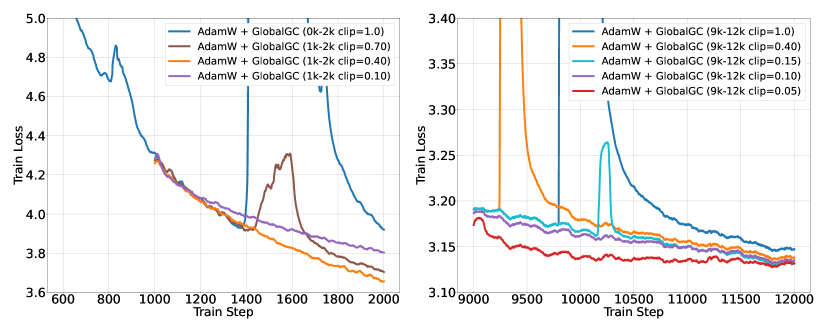
(a) Temporal threshold adaptation necessity: Fixed thresholds (0.4) prevent early spikes but fail later (10k steps), requiring dynamic adjustment.

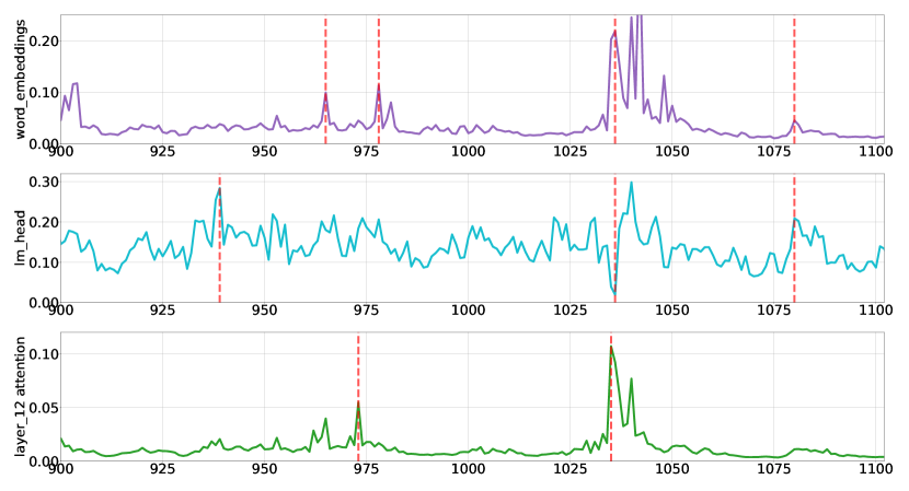
(b) Spikes in gradient norms occur at different training steps across parameters, indicating heterogeneous gradient behaviors.

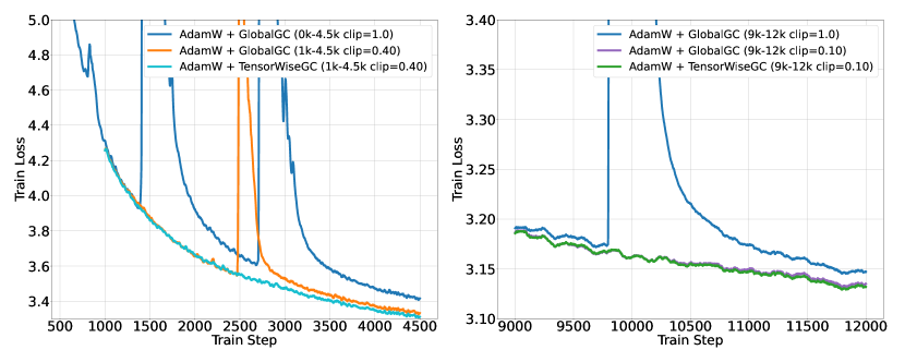
(c) Per-parameter gradient clipping mitigates loss spikes that global clipping cannot, leading to faster convergence.

Figure 1: Empirical motivation for AdaGC: (a) Temporal threshold decay necessitates adaptive clipping, (b) Parameter-specific gradient spikes demand localized control, (c) Fine-grained clipping outperforms global approaches.

In this section, we will introduce some phenomena of gradient clipping that motivate the design of the algorithm.

Adaptivity: The magnitudes of gradients in neural network training exhibit dynamic variations throughout the learning process. This renders fixed gradient clipping thresholds suboptimal for mitigating loss spikes, as demonstrated in Figure 1(a). While a threshold of 0.4 successfully mitigates loss spike during the initial training phase of the GPT-2 345M model, it becomes ineffective against the severe loss spike occurring around 10,000 iterations, where a substantially reduced threshold is required for stabilization. This phenomenon correlates with the observation that optimal clipping thresholds for convergence speed are strongly influenced by recent gradient norms (see corresponding subfigures). Motivated by these findings, we propose an adaptive clipping mechanism using the exponential moving average of gradient magnitudes as the per-step clipping threshold.

Locality: Figure 1(b) reveals that different parameters exhibit divergent gradient behaviors, with spikes occurring at distinct training phases. Using a global clipping threshold can degrade the convergence speed of certain parameters. Therefore, we propose replacing global gradient norm clipping with per-parameter norm clipping, where clipping is applied independently to each parameter. Furthermore, as illustrated in Figure 1(c), we evaluate the effectiveness of per-parameter clipping thresholds categorized by specific ratios on GPT2-345M. The results indicate that, under the same global gradient norm conditions, per-parameter clipping can address spike phenomena that global clipping cannot resolve, and achieve faster convergence speeds.

These observations collectively motivate our two core design principles: adaptive thresholding to address temporal gradient norm decay, and localized control to handle parameter-wise gradient heterogeneity. The dynamic nature of optimal clipping thresholds (Figure 1(a)) necessitates our exponential moving average mechanism for temporal adaptation, while asynchronous parameter gradient spikes (Figure 1(b)) justify per-parameter clipping granularity. Together, these principles form the foundation of AdaGC - adaptively adjusting localized thresholds that respect both the temporal evolution and spatial distribution of gradients.

4 Methodology: AdaGC

4.1 Preliminaries

Notations. Let $x_{t}\in\mathbb{R}^{d}$ denote a parameter vector where $x_{t}^{j}$ represents its $j$-th coordinate for $j\in[d]$. We write $\nabla_{x}f(x)$ for the gradient of any differentiable function $f:\mathbb{R}^{d}\rightarrow\mathbb{R}$, and use $u^{2}$ and $u/v$ to denote element-wise square and division operations for vectors $u,v\in\mathbb{R}^{d}$. The $\ell_{2}$-norm and $\ell_{\infty}$-norm are denoted by $\|\cdot\|$ and $\|\cdot\|_{\infty}$, respectively. For asymptotic comparisons, we write $f=\mathcal{O}(g)$ if $\exists c>0$ such that $f(x)\leq cg(x)$ for all $x$ in the domain.

Gradient Clipping Fundamentals. Consider a stochastic optimization problem with parameters $\theta\in\mathbb{R}^{d}$ and loss function $f(\theta;X_{t})$ evaluated on mini-batch $X_{t}$ at step $t$. Standard gradient descent updates follow:

$$\theta_{t}=\theta_{t-1}-\alpha\nabla_{\theta}f(\theta_{t-1},X_{t})$$ (1)

To prevent unstable updates from gradient explosions, gradient clipping (Pascanu et al., 2013) modifies the update rule as:

$$\begin{array}[]{c}\theta_{t}=\theta_{t-1}-\alpha h_{t}\nabla_{\theta}f(\theta_{t-1},X_{t})\\[3.99994pt] \text{ where }h_{t}:=\min\left\{\frac{\lambda_{abs}}{\|\nabla_{\theta}f(\theta_{t-1};X_{t})\|},1.0\right\}\end{array}$$ (2)

Here $\lambda_{\text{abs}}$ is an absolute clipping threshold requiring careful tuning. Our work focuses on norm-based clipping (scaling entire gradients exceeding $\lambda_{\text{abs}}$) rather than value-based clipping (element-wise truncation).

4.2 Adaptive Gradient Clipping based on Local Gradient Norm

This section introduces a novel gradient clipping strategy termed Adaptive Gradient Clipping (AdaGC), which distinguishes itself by not relying on a global gradient norm. Instead, AdaGC focuses on the local gradient norm of each parameter and utilizes a dynamic adaptive mechanism for gradient clipping. The proposed method employs an Exponential Moving Average (EMA) mechanism to maintain smoothed estimates of historical gradient norms per parameter, thus enhancing the accuracy of anomalous gradient detection and enabling independent clipping adjustments tailored to each parameter’s specific conditions. EMA is widely used in deep learning, and within AdaGC, it facilitates the balancing of historical and current gradient norms. The formulation is as follows:

$$\begin{array}[]{c}\boldsymbol{g}_{t,i}\leftarrow h_{t,i}\cdot\boldsymbol{g}_{t,i},\text{where }h_{t,i}=\min\left\{\lambda_{rel}\frac{\gamma_{t-1,i}}{\|\boldsymbol{g}_{t,i}\|},1.0\right\},\\[10.00002pt] \gamma_{t,i}=\beta\gamma_{t-1,i}+(1-\beta)\|\boldsymbol{g}_{t,i}\|.\end{array}$$ (3)

Here, $\lambda_{rel}$ is a predefined relative clipping threshold, $\boldsymbol{g}_{t,i}$ represents the gradient of the $i$-th parameter at time step $t$, and $h_{t,i}$ is a clipping function activated when $\|\boldsymbol{g}_{t,i}\|>\lambda_{rel}\cdot\gamma_{t-1,i}$, thereby scaling the gradient norm to $\lambda_{rel}\cdot\gamma_{t-1,i}$. Additionally, $\beta$ is the smoothing coefficient for EMA. We consistently incorporate the clipped gradient norm into the historical observations rather than the pre-clipped values.

Despite its simplicity, AdaGC adaptively adjusts based on the magnitude of each parameter’s gradient norm. Whenever the gradient norm at a current timestep exceeds a predefined range of average norms within a historical window, it effectively suppresses these outlier gradients.

However, during the initial stages of model training (e.g., the first 100 steps), the gradient norms are typically large and fluctuate significantly, indicating a substantial decreasing trend. Direct application of AdaGC during this period could lead to two issues: first, erroneously accumulating the early large gradient norms into the historical values, resulting in compounded errors; second, compared to traditional global-norm-based methods, AdaGC might delay clipping, thus potentially slowing down the loss reduction. To address these issues, we introduce a hyperparameter $T_{start}$(default set to 100), representing a warm-up period during which traditional global gradient norm clipping is applied.

Additionally, the AdaGC strategy can be seamlessly integrated with various optimizers, such as AdamW (Loshchilov & Hutter, 2017), enhancing its practicality and flexibility. Algorithm 1 demonstrates its implementation with the AdamW optimizer.

Overall, AdaGC offers a more precise and effective gradient management method for large-scale model training, contributing to improved training stability and performance.

Algorithm 1 AdamW with AdaGC

1:  given: $\{\alpha_{t}\}_{t=1}^{T},\lambda_{w},\epsilon_{1},\beta_{1},\beta_{2},{\color[rgb]{0,0,1}\beta}\in[0,1),{\color[rgb]{0,0,1}\lambda_{abs}},{\color[rgb]{0,0,1}T_{start}}$

2:  initialize: $\boldsymbol{\theta}_{0},m_{0}\leftarrow 0,v_{0}\leftarrow 0,t\leftarrow 0$

3:  repeat

4:  compute $\boldsymbol{g}_{t}$ = $\nabla_{\boldsymbol{\theta}}f_{t}(\boldsymbol{\theta}_{t-1},X_{t})$

5:  if $t<T_{start}$ then

6:   ${\color[rgb]{0,0,1}h_{t}=\min\left\{\frac{\lambda_{abs}}{\|\boldsymbol{g}_{t}\|},1.0\right\}}$

7:   ${\color[rgb]{0,0,1}\widehat{\boldsymbol{g}_{t}}=h_{t}\cdot\boldsymbol{g}_{t}}$

8:   for $i\in|\boldsymbol{\theta}|$ do

9:    ${\color[rgb]{0,0,1}\gamma_{t,i}=\min\left\{\gamma_{t-1,i},\|\widehat{\boldsymbol{g}_{t,i}}\|\right\},\gamma_{0,i}=\|\widehat{\boldsymbol{g}_{1,i}}\|}$

10:   end for

11:  else

12:   for $i\in|\boldsymbol{\theta}|$ do

13:    ${\color[rgb]{0,0,1}h_{t,i}=\min\left\{\lambda_{rel}\frac{\gamma_{t-1,i}}{\|\boldsymbol{g}_{t,i}\|},1.0\right\}}$

14:    ${\color[rgb]{0,0,1}\widehat{\boldsymbol{g}_{t,i}}=h_{t,i}\cdot\boldsymbol{g}_{t,i}}$

15:    ${\color[rgb]{0,0,1}\gamma_{t,i}=\beta\gamma_{t-1,i}+(1-\beta)\|\widehat{\boldsymbol{g}_{t,i}}\|}$

16:   end for

17:  end if

18:  $\boldsymbol{m}_{t}=\beta_{1}\boldsymbol{m}_{t-1}+(1-\beta_{1}){\color[rgb]{0,0,1}\widehat{\boldsymbol{g}_{t}}}$

19:  $\boldsymbol{v}_{t}=\beta_{2}\boldsymbol{v}_{t-1}+(1-\beta_{2}){\color[rgb]{0,0,1}\widehat{\boldsymbol{g}_{t}}}^{2}$

20:  $\widehat{\boldsymbol{m}_{t}}=\boldsymbol{m}_{t}/(1-\beta_{1}^{t}),\quad\widehat{\boldsymbol{v}_{t}}=\boldsymbol{v}_{t}/(1-\beta_{2}^{t})$

21:  $\boldsymbol{\theta}_{t}=\boldsymbol{\theta}_{t-1}-\alpha_{t}\lambda_{w}\boldsymbol{\theta}_{t-1}-\alpha_{t}\widehat{\boldsymbol{m}_{t}}/(\sqrt{\widehat{\boldsymbol{v}_{t}}}+\epsilon_{1})$

22:  until $\boldsymbol{\theta}_{t}$ not converge

4.3 Convergence Analysis

In this section, we give the convergence guarantee of Adam with AdaGC stated as follows:

Theorem 4.1.

Under mild assumptions, by selecting $\alpha_{t}=\mathcal{O}(1/\sqrt{T})$, $\beta_{2}=1-\mathcal{O}(1/T)$ and $\beta_{1}<\sqrt{\beta_{2}}$, when $\tau$ is randomly chosen from $\{1,2,\cdots,T\}$ with equal probabilities, it holds that

$$\mathbb{E}\|\nabla f(\theta_{\tau})\|^{2}=\mathcal{O}\left(\frac{1}{\sqrt{T}}\right).$$

Theorem 4.1 shows that even with local clipped gradient, Adam with AdaGC can converge in the same rate as vanilla Adam. Due to the limited space the formal assumptions, theorem statement with detailed proof can be found in Appendix A.

5 Experiments

This paper primarily focuses on the pre-training of large language models, using Llama-2 (Touvron et al., 2023b) as our primary experimental subject. Experiments were conducted using NVIDIA GPU A100 40G. Moreover, our proposed method demonstrates strong generalization across various VLM models, achieving robust results.

Table 1: Zero-shot performance of Llama-2 7B on WikiText and LAMBADA datasets.

	Metrics	GlobalGC	AdaptiveGradientClip	StableAdamW	AdaGC-Shard	AdaGC
WikiText	Word PPL $\downarrow$	21.173	21.467	21.733	20.878	20.434
	Byte PPL $\downarrow$	1.770	1.774	1.778	1.765	1.758
LAMBADA	ACC $\uparrow$	49.35 ($\pm$ 0.70)	49.27 ($\pm$ 0.70)	48.96 ($\pm$ 0.70)	47.76 ($\pm$ 0.70)	49.49 ($\pm$ 0.70)
	PPL $\downarrow$	11.111 ($\pm$ 0.334)	11.509 ($\pm$ 0.354)	11.774 ($\pm$ 0.363)	11.518 ($\pm$ 0.341)	10.515 ($\pm$ 0.315)

5.1 Experimental Setup

Models and Datasets: We evaluated the efficacy of AdaGC on various Llama-2 models including Tiny, 7B and 13B. The C4-en (Raffel et al., 2020) dataset, a clean corpus of English text extracted from Common Crawl, served as our pre-training dataset. We assessed model performance by computing perplexity on the WikiText (Merity et al., 2016) and LAMBADA (Paperno et al., 2016) datasets. We also conducted experiments on GPT-2 (Radford et al., 2019) and CLIP (Radford et al., 2021) models to further validate AdaGC’s generalization capabilities.

Comparison Methods: We selected several techniques including Global Gradient Clipping (GlobalGC for short) (Pascanu et al., 2013), Adaptive Gradient Clipping (Brock et al., 2021), StableAdamW (Wortsman et al., 2023a), and Scaled Embed (Takase et al., 2023) from different approaches such as gradient clipping, update clipping, and parameter initialization for comparison.

Training Details: Pre-training large scale models, particularly Llama-2 7B and 13B, is typically resource-intensive. Like StableAdamW (Wortsman et al., 2023a) and Scaled Embed (Takase et al., 2023), our primary focus was to explore training instability rather than achieve ultimate accuracy. For ease of multiple experiments, we conducted 9,000 training steps on 36 billion tokens for both Llama-2 7B and 13B models, and 36,000 steps on 36 billion tokens for the Llama-2 Tiny model. For additional details on the hyperparameters, please refer to the Appendix B.

Critical Hyperparameter Selection. We conducted a systematic study to evaluate the two critical hyperparameters in AdaGC: the EMA coefficient $\beta$ and the relative clipping threshold $\lambda_{rel}$. Our analysis utilized coordinate descent (Bertsekas, 1997) for hyperparameter optimization on the Llama-2 Tiny model. Initially, we examined the relative clipping threshold $\lambda_{rel}$ with a fixed EMA coefficient $\beta=0.98$, testing the values $\{1.01,1.05,1.10\}$. As depicted in Figure 2(a), $\lambda_{rel}=1.05$ achieved optimal performance by effectively balancing gradient regulation effectiveness (compromised at $\lambda_{rel}\geq 1.10$) and update stability (degraded at $\lambda_{rel}\leq 1.01$). With this optimal threshold established, we proceeded to investigate the EMA smoothing factor $\beta\in\{0.95,0.98,0.99\}$. Figure 2(b) demonstrates that $\beta=0.98$ provides superior adaptation speed while maintaining historical consistency, yielding the best performance. Consequently, we adopted the parameter settings $\lambda_{rel}=1.05$ and $\beta=0.98$ for all subsequent experiments reported in this paper.

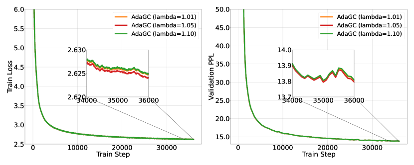
(a) Relative clipping threshold $\lambda_{\text{rel}}$.

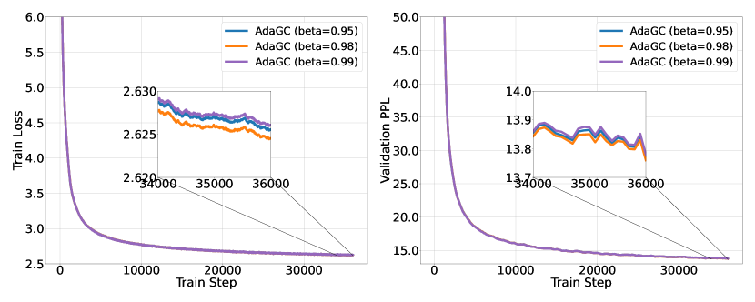
(b) EMA coefficient $\beta$.

Figure 2: Study of AdaGC’s hyperparameters on Llama-2 Tiny. (a) Relative clipping threshold analysis demonstrates $\lambda_{\text{rel}}=1.05$ achieves optimal gradient regulation. (b) EMA coefficient analysis reveals $\beta=0.98$ best balances historical consistency with rapid adaptation.

5.2 Experimental Results

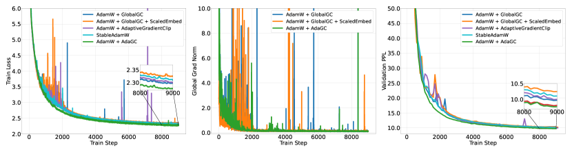
(a) Llama-2 7B training dynamics: AdaGC (green) eliminates loss spikes observed in baseline methods (GlobalGC-blue, ScaledEmbed-orange, AdaptiveGradientClip-purple, StableAdamW-cyan), achieving final training loss 0.02 lower than GlobalGC. Validation perplexity (right) shows correlated improvement with stable gradient norms (middle).

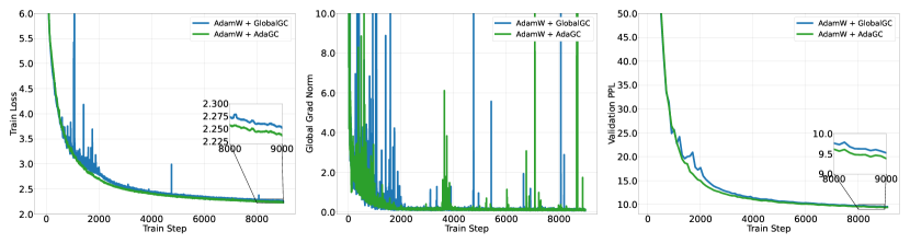
(b) Llama-2 13B scalability analysis: AdaGC maintains superior stability at scale, reducing training loss and validation perplexity by 0.64% and 1.47% respectively versus GlobalGC, demonstrating method scalability.

Figure 3: Large language model training analysis: (a) 7B model comparison shows AdaGC’s loss spike elimination and performance gains, (b) 13B results demonstrate method scalability.

Our comprehensive evaluation demonstrates AdaGC’s effectiveness across model scales and architectures. Figure 3 presents comparative results on Llama-2 7B and 13B models, analyzing training dynamics through loss trajectories, gradient norms, and validation perplexities. For the 7B model, baseline methods (GlobalGC, Scaled Embed, Adaptive Gradient Clipping, and StableAdamW) exhibit frequent loss spikes during training, while AdaGC completely eliminates these instability events. This stability translates to measurable performance gains, with AdaGC achieving a 0.02 lower final training loss (2.28 vs 2.30) and 2.1% reduced validation perplexity compared to the strongest baseline (GlobalGC).

The approach demonstrates strong scalability on the Llama-2 13B model, where AdaGC eliminates loss spikes entirely compared to GlobalGC. Qualitative analysis reveals AdaGC’s superior outlier gradient management, maintaining smoother loss trajectories throughout training. This enhanced stability yields concrete performance improvements: 0.65% lower training loss (absolute difference of 0.0146) and 1.47% reduced validation perplexity relative to GlobalGC.

Downstream zero-shot evaluation on WikiText and LAMBADA datasets (Table 1) confirms the practical benefits of stable training. AdaGC achieves state-of-the-art performance across all benchmarks, reducing WikiText perplexity by 3.5% (20.434 vs 21.173) while improving LAMBADA accuracy by 0.14 percentage points (49.49% vs 49.35%) compared to GlobalGC. These results establish a direct correlation between training stability and final model quality.

To validate architectural generality, we extend evaluation to vision-language pretraining with CLIP ViT-Base. As shown in Figure 4(a), AdaGC completely eliminates loss spikes observed in vision-specific stabilization methods while achieving 25% faster convergence than StableAdamW (reaching target loss in 15k vs 20k steps). The improved training dynamics translate to superior zero-shot recognition performance (Figure 4(b)), with AdaGC demonstrating consistent accuracy gains across modalities - including a 0.27 percentage point improvement on ImageNet-1K (39.84% vs 39.57%) over GlobalGC.

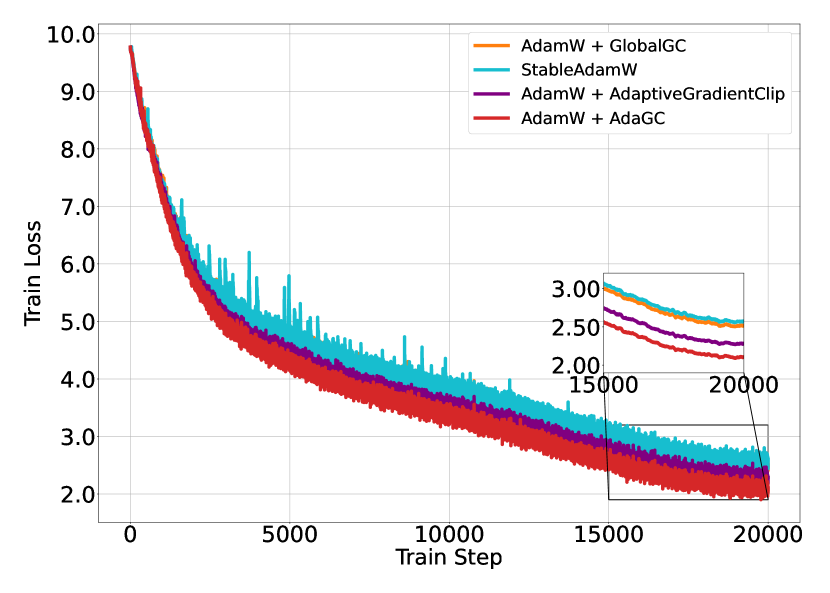
(a)

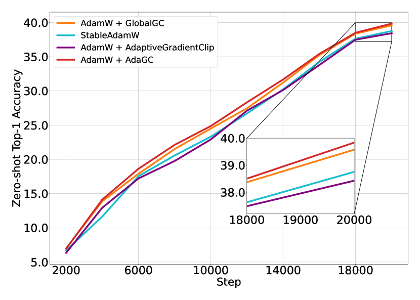
(b)

Figure 4: CLIP ViT-Base results: (a) Training loss trajectory comparison. AdaGC achieves 25% faster convergence (15k vs 20k steps) with complete loss spike elimination compared to StableAdamW. (b) Zero-shot recognition performance. Final accuracy improves 0.27pp (39.84% vs 39.57%) on ImageNet-1K, demonstrating cross-modal generalization.

5.3 Ablation Study

We conduct systematic ablation studies across three critical dimensions of AdaGC: (1) EMA gradient norm initialization strategies, (2) adaptivity efficacy, and (3) locality granularity. The adaptivity property has been empirically validated through experimental analysis (Section 3) and comprehensive experimental results across all benchmarks.

EMA Initialization Strategy.

The initialization of EMA gradient norms requires careful design due to large initial gradient fluctuations during early training phases (first 100 steps). We evaluate five initialization variants on GPT-2 345M: The default AdaGC strategy employs GlobalGC during warm-up while tracking minimum per-parameter norms ($\gamma_{t,i}=\min(\|\boldsymbol{g}_{t,i}\|,\gamma_{t-1,i})$). Comparative approaches include: (1) norm initialization without GlobalGC warm-up (directly using $\gamma_{t,i}=\min(\|\boldsymbol{g}_{t,i}\|,\gamma_{t-1,i})$ from step 0), (2) constant initialization ($\gamma_{0,i}\in\{0.5,1.0\}$), and (3) thresholded initialization ($\gamma_{t,i}=\min(\|\boldsymbol{g}_{t,i}\|,0.1)$). Figure 6(b) demonstrates that while all variants eliminate loss spikes, convergence quality varies within 0.36%. The default strategy achieves optimal final loss (2.9708 vs 2.9725 for next-best), showing that GlobalGC-guided warm-up better preserves parameter update consistency than direct initialization. This establishes the importance of phased initialization for gradient norm adaptation.

Locality Granularity. We analyze clipping granularity across three implementation levels. Global-level clipping applies a single threshold for the entire model, while parameter-wise adaptation operates per individual parameter. On GPT-2 345M (Figure 5(a)), global clipping reduces but fails to eliminate spikes (1 event vs 0 for parameter-wise), with 0.25% (2.9639 vs 2.9712) higher final loss.

As model scale increases to 7B parameters, TensorParallel distributed training becomes necessary for efficient optimization. We therefore evaluate shard-wise adaptation on Llama-2 7B, where parameters are partitioned across devices and clipping operates per-shard. Figure 5(b) reveals that while shard-wise clipping eliminates spikes, it introduces parameter update inconsistencies across devices, increasing loss variance by 4.3% (2.3836 vs 2.28) compared to parameter-wise granularity. This degradation stems from independent clipping of parameter shards disrupting holistic parameter updates.

These results establish parameter-wise granularity as optimal, achieving precise adaptation while maintaining parameter update coherence across distributed systems.

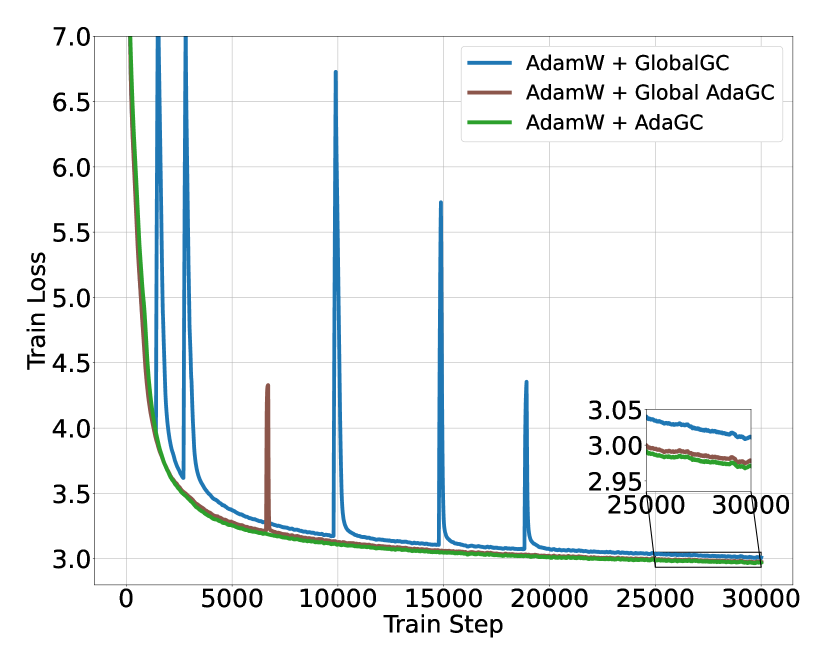
(a)

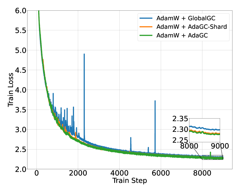
(b)

Figure 5: Locality granularity analysis: (a) Global vs parameter-wise clipping on GPT-2 345M model demonstrates spike elimination capability, (b) Distributed shard-wise clipping on 7B model reveals parameter integrity requirements.

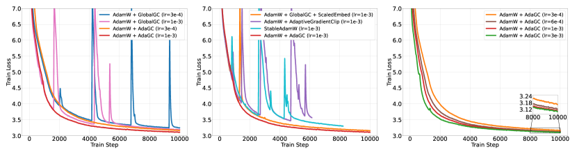
(a)

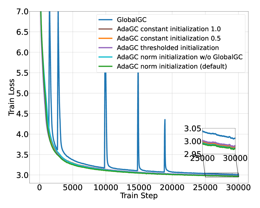
(b)

Figure 6: (a) Large rate tolerance on GPT-2 345M: AdaGC enables stable training at 10$\times$ learning rate (left), outperforms baselines (mid), and accelerates convergence through rate scaling (right). (b) EMA initialization strategies.

5.4 Exploring AdaGC’s Capabilities

We demonstrate AdaGC’s potential advantages over global gradient clipping through three critical dimensions: large learning rate tolerance, batch size scalability, and optimizer compatibility.

Large Learning Rate Tolerance

Figure 6(a) analyzes training stability under aggressive learning rate regimes using GPT-2 345M. At $3\times 10^{-3}$ learning rate (10$\times$ baseline), AdaGC maintains stable training (0 loss spikes) while achieving 2.52% lower final loss than GlobalGC (left panel). Comparative analysis with stabilization baselines (middle panel) reveals AdaGC’s unique capability: 1.52% lower training loss than GlobalGC+ScaledEmbed (best competitor) without spike mitigation overhead. The scaling law analysis (right panel) suggests a noticeable convergence acceleration with increasing learning rates (from $3\times 10^{-4}$ to $3\times 10^{-3}$). This indicates that learning rate scaling may contribute to a faster training process, albeit not with a perfect linear relationship.

Batch Size Scalability

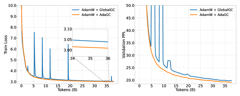
(a) batch size = $512$, lr = $3.0\times 10^{-4}$

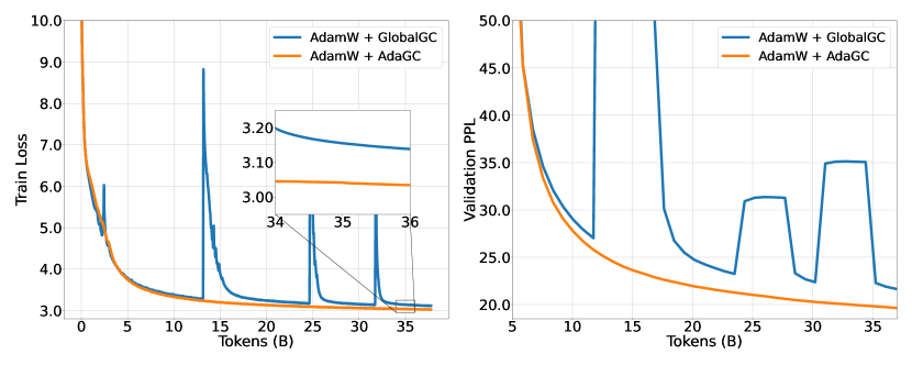
(b) batch size = $2048$, lr = $6.0\times 10^{-4}$

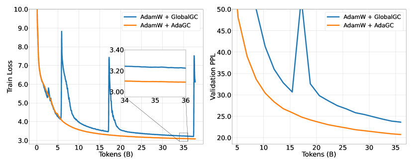
(c) batch size = $4096$, lr = $8.5\times 10^{-4}$

(d) batch size = $8192$, lr = $1.2\times 10^{-3}$

Figure 9: AdaGC’s large-batch scalability on GPT-2 345M: Maintains 0 loss spikes (vs GlobalGC’s 100% rate) with batch sizes up to 8192 (16$\times$ baseline) and proportional learning rate scaling, achieving 1.28%-19.55% perplexity reduction.

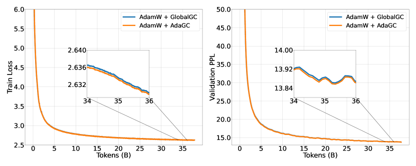
(a) batch size = $512$, lr = $3.0\times 10^{-4}$

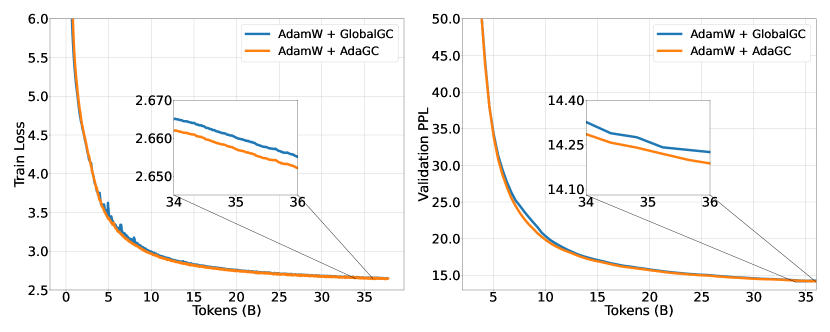
(b) batch size = $2048$, lr = $6.0\times 10^{-4}$

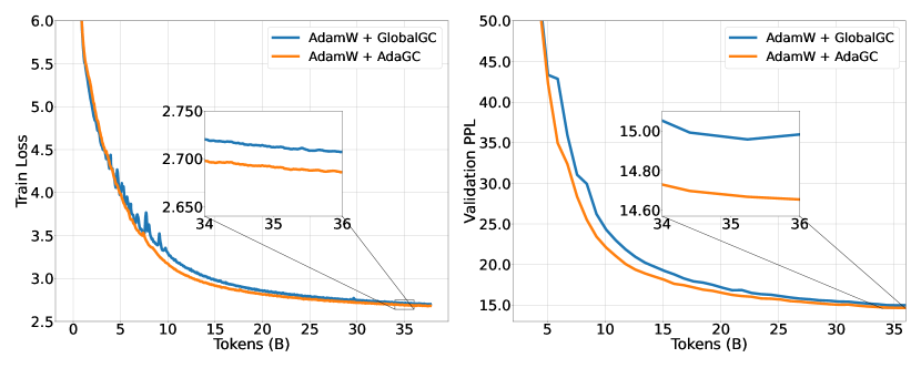
(c) batch size = $4096$, lr = $8.5\times 10^{-4}$

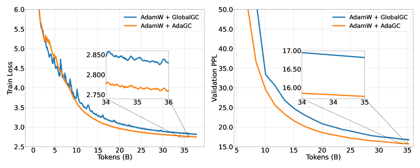
(d) batch size = $8192$, lr = $1.2\times 10^{-3}$

Figure 10: AdaGC’s large-batch scalability on Llama-2 Tiny: Cross-architecture validation shows 6.19% lower perplexity at 8192 batch size.

Figure 7 validates AdaGC’s effectiveness under scaled batch training paradigms. With batch sizes up to 8192 (16$\times$ baseline) and proportional learning rate scaling, AdaGC maintains perfect stability (0 spikes vs 100% spike rate for GlobalGC) while reducing final perplexity by 1.28% - 19.55% across configurations. The Llama-2 Tiny experiments confirm cross-architecture effectiveness, showing 6.19% lower perplexity than GlobalGC at a batch size of 8192. This demonstrates AdaGC’s capability to enable efficient large-batch distributed training without stability compromises. Additional details can be found in Figure 9 and Figure 10 in Appendix D.

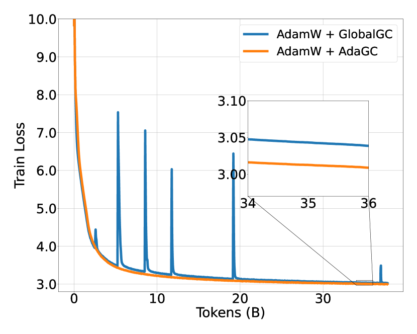
(a) bs = $512$, lr = $3.0\times 10^{-4}$

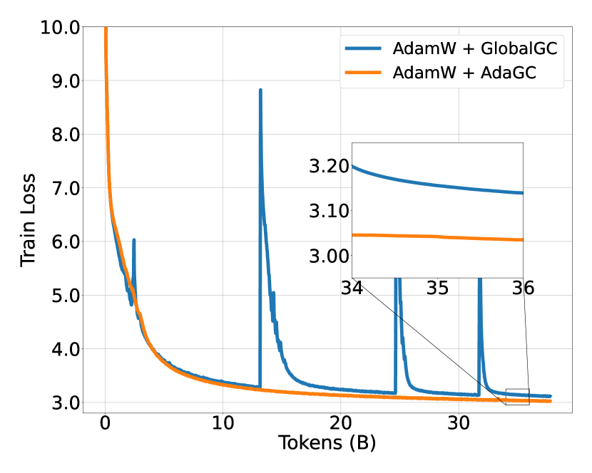
(b) bs = $2048$, lr = $6.0\times 10^{-4}$

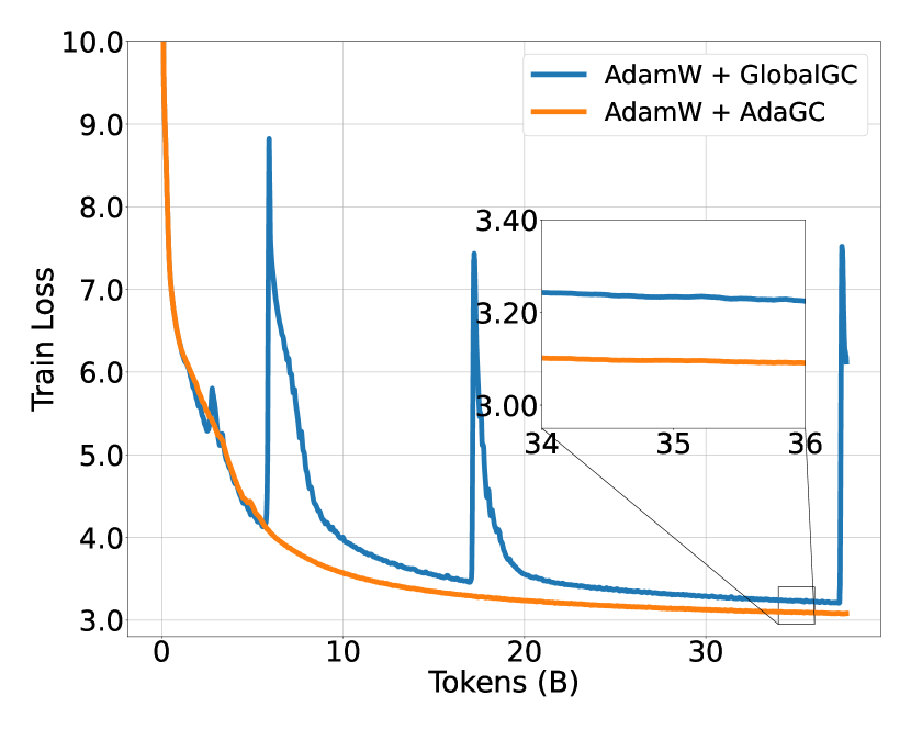
(c) bs = $4096$, lr = $8.5\times 10^{-4}$

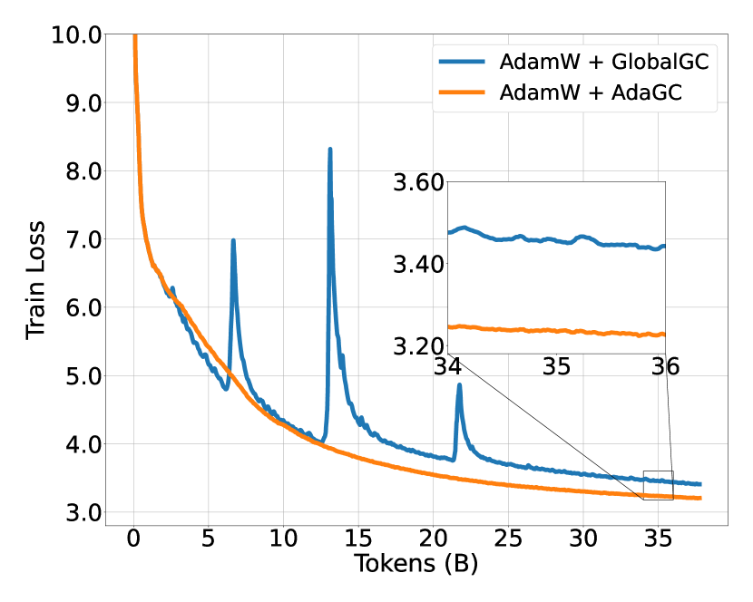
(d) bs = $8192$, lr = $1.2\times 10^{-3}$

Figure 7: AdaGC’s large-batch scalability on GPT-2 345M: Maintains 0 loss spikes (vs GlobalGC’s 100% rate) with batch sizes up to 8192 (16$\times$ baseline).

Optimizer Compatibility

Figure 8 demonstrates AdaGC’s generalization across optimization frameworks. Integrated with Lion, AdaGC achieves comparable training loss to GlobalGC (1.9912 vs 2.0165) while improving ImageNet-1K top-1 accuracy by 0.16 percentage points (40.81% vs 40.65%). When combined with StableAdamW (which explicitly avoids gradient clipping), AdaGC provides additional 19.23% training loss reduction (2.0523 vs 2.5412) and 0.96 percentage point accuracy gain (39.71% vs 38.75%), establishing complementary benefits. These results position AdaGC as a universal stabilization component for modern optimization paradigms.

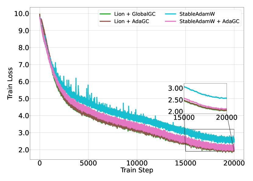
Figure 8: AdaGC’s optimizer compatibility on CLIP ViT-Base: With Lion, achieves 0.16pp higher accuracy (40.81% vs 40.65%) at comparable loss; Combined with StableAdamW, reduces loss by 19.23% (2.0523 vs 2.5412) with 0.96pp accuracy gain. Demonstrates universal stabilization across optimization frameworks.

6 Discussion

6.1 Socio-Economic Value

Pre-training large models entails substantial costs and is vulnerable to significant economic losses due to instabilities in the training process. Loss spikes, typically addressed by resuming training from the latest checkpoint as illustrated by the PaLM (Chowdhery et al., 2023) approach, can have severe economic impacts. According to the MegaScale (Jiang et al., 2024) report, the average recovery time from an interruption is about 15 minutes. Considering the Llama-3  model, which utilizes 16,000 NVIDIA H100 GPUs priced between $2.29 to $2.49 per hour , each interruption due to a Loss Spike can lead to direct economic losses ranging from approximately $9,160 to $9,960. Our proposed adaptive gradient clipping method effectively reduces the frequency of Loss Spikes, thereby enhancing training stability and minimizing economic waste.

6.2 Limitations

Resource constraints prevented this study from conducting long-term training experiments on the Llama-2 open-source model. However, our internal business validations indicate that the method remains effective throughout the mid to late stages of training. Future plans, resources permitting, include conducting comprehensive experiments on the Llama-2 model and sharing the findings with the academic community.

7 Conclusion

This paper systematically addresses the critical challenge of loss spikes in large model pre-training through gradient dynamics analysis. Our key insight reveals two limitations in conventional approaches: temporal gradient norm decay requires adaptive thresholds, while parameter-specific gradient heterogeneity demands localized control. These findings motivate AdaGC, which integrates exponential moving average-based threshold adaptation with per-parameter clipping while maintaining Adam-comparable $\mathcal{O}(1/\sqrt{T})$ convergence rate - proving local clipping preserves theoretical convergence properties. Comprehensive experiments demonstrate AdaGC’s dual benefits: complete loss spike elimination across LLMs (3.5% WikiText perplexity reduction on Llama-2 7B) and LVLMs (25% faster CLIP convergence than StableAdamW), coupled with enhanced training stability and final model quality. The consistent success across architectures and optimizers validates that jointly addressing temporal adaptation and spatial parameter characteristics provides an effective stabilization paradigm for large-scale training.

Impact Statement

This paper presents work whose goal is to advance the field of Machine Learning. There are many potential societal consequences of our work, none which we feel must be specifically highlighted here.

Appendix A Convergence Proof

In this section, we provide the necessary assumptions and lemmas for the proofs of Theorem 4.1.

Notations

The $k$-th component of a vector $v_{t}$ is denoted as ${v}_{t,k}$. Other than that, all computations that involve vectors shall be understood in the component-wise way. We say a vector $v_{t}\geq 0$ if every component of $v_{t}$ is non-negative, and $v_{t}\geq w_{t}$ if $v_{t,k}\geq w_{t,k}$ for all $k=1,2,\ldots,d$. The $\ell_{1}$ norm of a vector $v_{t}$ is defined as $\|v_{t}\|_{1}=\sum_{k=1}^{d}|{v}_{t,k}|$. The $\ell_{2}$ norm is defined as $\|v_{t}\|^{2}=\langle v_{t},v_{t}\rangle=\sum_{k=1}^{d}|{v}_{t,k}|^{2}$. Given a positive vector $\hat{\eta}_{t}$, it will be helpful to define the following weighted norm: $\|v_{t}\|^{2}_{\eta_{t}}=\langle v_{t},\hat{\eta}_{t}v_{t}\rangle=\sum_{k=1}^{d}\hat{\eta}_{t,k}|{v}_{t,k}|^{2}$.

Assumption A.1.

The function f is lower bounded by $\underline{f}$ with L-Lipschitz gradient.

Assumption A.2.

The gradient estimator $g$ is unbiased with bounded norm, e.g,

$$\begin{split}&\mathbb{E}[g|x_{t}]=\nabla f(x_{t}),\ \|g_{t}\|\leq G.\end{split}$$

Assumption A.3.

The coefficient of clipping $h_{t,i}$ is lower bounded by some $h_{0}>0$.

Assumption A.4.

$\|g_{t}-\nabla f(x_{t})\|\leq p\|\nabla f(x_{t})\|$ holds for some $p<1$ and for all t.

Remark A.5.

Assumption A.1 and Assumption A.2 are widely used in the proof of optimization algorithm with adaptive learning rates (Reddi et al., 2018). Assumption A.3 is because the gradient norm changes slowly when training the neural network, and the last assumption holds when the batch size is large enough.

Lemma A.6.

Let $\zeta:=\beta_{1}^{2}/{\beta_{2}}$. We have the following estimate

$$m_{t}^{2}\leq\frac{1}{(1-\zeta)(1-\beta_{2})}v_{t},~\forall t.$$ (4)

Proof.

By the iteration formula $m_{t}=\beta_{1}m_{t-1}+(1-\beta_{1})\hat{g}_{t}$ and $m_{0}=0$, we have

$$m=\sum_{i=1}^{t}\beta_{1}^{t-i}(1-\beta_{1})\hat{g}_{i}.$$

Similarly, by $v_{t}=\beta_{2}v_{t-1}+(1-\beta_{2})\hat{g}_{t}^{2}$ and $v_{0}=0$, we have

$$v_{t}=\sum_{i=1}^{t}\beta_{2}^{t-i}(1-\beta_{2})\hat{g}_{i}^{2}$$

It follows by arithmetic inequality that

$$\begin{split}m_{t}^{2}&=\left(\sum_{i=1}^{t}\frac{(1-\beta_{1})\beta_{1}^{t-i}}{\sqrt{(1-\beta_{2})\beta_{2}^{t-i}}}\sqrt{(1-\beta_{2})\beta_{2}^{t-i}}\hat{g}_{i}\right)^{2}\\ &\leq\left(\sum_{i=1}^{t}\frac{(1-\beta_{1})^{2}\beta_{1}^{2(t-i)}}{(1-\beta_{2})\beta_{2}^{t-i}}\right)\left(\sum_{i=1}^{t}(1-\beta_{2})\beta_{2}^{t-i}\hat{g}_{i}^{2}\right)=\left(\sum_{i=1}^{t}\frac{(1-\beta_{1})^{2}\beta_{1}^{2(t-i)}}{(1-\beta_{2})\beta_{2}^{t-i}}\right)v_{t}.\end{split}$$

Further, we have

$$\sum_{i=1}^{t}\frac{(1-\beta_{1})^{2}\beta_{1}^{2(t-i)}}{(1-\beta_{2})\beta_{2}^{t-i}}\leq\frac{1}{1-\beta_{2}}\sum_{i=1}^{t}\left(\frac{\beta_{1}^{2}}{\beta_{2}}\right)^{t-i}=\frac{1}{1-\beta_{2}}\sum_{k=0}^{t-1}\zeta^{k}\leq\frac{1}{(1-\zeta)(1-\beta_{2})}.$$

The proof is completed. ∎

Lemma A.7.

The following estimate holds

$$\sum_{t=1}^{T}\|\Delta_{t}\|^{2}\leq\frac{\alpha^{2}G^{2}}{\epsilon}$$

Proof.

By using the definition of $m_{t}$, it holds $\|m_{t}\|^{2}\leq G^{2}$.

Then, $\|\Delta_{t}\|^{2}=\|\frac{\alpha_{t}m_{t}}{\sqrt{v_{t}}+\epsilon}\|^{2}\leq\frac{G^{2}}{\epsilon}\alpha_{t}^{2}$ by using the definition of $\Delta_{t}$.

Therefore, $\small\sum_{t=1}^{T}\|\Delta_{t}\|^{2}\leq\frac{G^{2}}{\epsilon}\sum_{t=1}^{T}\frac{\alpha^{2}}{T}=\frac{G^{2}\alpha^{2}}{\epsilon}$.

∎

Lemma A.8.

With the Assumption A.3 and A.4, it holds that

$$\mathbb{E}\left\langle\nabla f\left(\theta_{t}\right),\hat{\eta}_{t}\hat{g}_{t}\right\rangle\geq h_{0}\mathbb{E}\left\|\nabla f\left(\theta_{t}\right)\right\|_{\hat{\eta}_{t}}^{2}.$$

Proof.

According to Assumption A.4, it holds that

$$\begin{split}\left\langle\nabla_{i}f\left(\theta_{t}\right),g_{t,i}\right\rangle&=-\frac{1}{2}\left(\left\|\nabla_{i}f\left(\theta_{t}\right)-g_{t,i}\right\|^{2}-\left\|\nabla_{i}f\left(\theta_{t}\right)\right\|^{2}-\left\|g_{t,i}\right\|^{2}\right)\\ &\geq(1-p^{2})\left\|\nabla_{i}f\left(\theta_{t}\right)\right\|^{2}\geq 0.\end{split}$$

Thus, it holds that

$$\begin{split}\mathbb{E}\left[\left\langle\nabla f(x_{t}),\hat{\eta}_{t}\hat{g}_{t}\right\rangle\right]&=\mathbb{E}\left[\sum_{i}\left\langle\nabla_{i}f(\theta_{t}),h_{t,i}\hat{\eta}_{t,i}g_{t,i}\right\rangle\right]\\ &\geq h_{0}\mathbb{E}\left[\sum_{i}\left\langle\nabla_{i}f(x_{t}),h_{t,i}\hat{\eta}_{t,i}g_{t,i}\right\rangle\right]\\ &=h_{0}\mathbb{E}\left\langle\nabla f(\theta_{t}),\hat{\eta}_{t}g_{t}\right\rangle=h_{0}\mathbb{E}\|\nabla f(\theta_{t})\|^{2}_{\hat{\eta}_{t}}.\end{split}$$

∎

Let $\Delta_{t}:=\theta_{t+1}-\theta_{t}=-\alpha_{t}m_{t}/(\sqrt{v_{t}}+\epsilon)$. Let $\hat{v}_{t}=\beta_{2}v_{t-1}+(1-\beta_{2})\delta_{t}^{2}$, where $\delta_{t}^{2}=\mathbb{E}_{t}\left[\hat{g}_{t}^{2}\right]$ and let $\hat{\eta}_{t}=\alpha_{t}/\sqrt{\hat{v}_{t}+\epsilon}$.

Lemma A.9.

Let $M_{t}=\mathbb{E}\left[\langle\nabla f(\theta_{t}),\Delta_{t}\rangle+L\|\Delta_{t}\|^{2}\right]$. Let $\alpha_{t}=\alpha/\sqrt{T}$ and $\beta_{2}=1-\beta/T$. Then, for $T\geq 1$ we have

$$\begin{split}\sum_{t=1}^{T}M_{t}\leq\frac{C_{2}}{1-\sqrt{\zeta}}+\frac{LG^{2}\alpha^{2}}{(1-\sqrt{\zeta})\epsilon}-\frac{(1-\beta_{1})h_{0}}{2}\sum_{t=1}^{T}\mathbb{E}\|\nabla f(\theta_{t})\|_{\hat{\eta}_{t}}^{2},\end{split}$$ (5)

where $C_{2}=\frac{5}{2(1-\beta_{1})h_{0}}\left((1-\beta_{1})^{2}\frac{4\alpha\beta G^{4}}{\epsilon^{3}}+\beta_{1}^{2}\alpha\beta\left(\frac{G^{4}}{\beta_{2}\epsilon^{3}}+\frac{(1+\epsilon)G^{2}}{(1-\zeta)\epsilon\beta_{2}}+\frac{G^{4}}{\beta_{2}}\right)\right).$

Proof.

To split $M_{t}$, firstly we introduce the following two equalities. Using the definitions of $v_{t}$ and $\hat{v}_{t}$, we obtain

$$\begin{split}\frac{\left(1-\beta_{1}\right)\alpha_{t}\hat{g}_{t}}{\sqrt{v_{t}}+\epsilon}&=\frac{\left(1-\beta_{1}\right)\alpha_{t}\hat{g}_{t}}{\sqrt{\hat{v}_{t}}+\epsilon}+\left(1-\beta_{1}\right)\alpha_{t}\hat{g}_{t}\left(\frac{1}{\sqrt{v_{t}}+\epsilon}-\frac{1}{\sqrt{\hat{v}_{t}}+\epsilon}\right)\\ &=\left(1-\beta_{1}\right)\hat{\eta}_{t}\hat{g}_{t}+\left(1-\beta_{1}\right)\alpha_{t}\hat{g}_{t}\frac{\left(1-\beta_{2}\right)\left(\sigma_{t}^{2}-\hat{g}_{t}^{2}\right)}{\left(\sqrt{v_{t}}+\epsilon\right)\left(\sqrt{\hat{v}_{t}}+\epsilon\right)\left(\sqrt{v_{t}}+\sqrt{\hat{v}_{t}}\right)}\\ &=\left(1-\beta_{1}\right)\hat{\eta}_{t}\hat{g}_{t}+\left(1-\beta_{1}\right)\hat{\eta}_{t}\hat{g}_{t}\frac{\left(1-\beta_{2}\right)\left(\sigma_{t}^{2}-\hat{g}_{t}^{2}\right)}{\left(\sqrt{v_{t}}+\epsilon\right)\left(\sqrt{v_{t}}+\sqrt{\hat{v}_{t}}\right)}\end{split}$$

In addition, we can obtain:

$$\begin{split}&\beta_{1}\alpha_{t}m_{t-1}\left(\frac{1}{\sqrt{\beta_{2}v_{t-1}}+\sqrt{\beta_{2}}\epsilon}-\frac{1}{\sqrt{v_{t}}+\epsilon}\right)\\ &=\beta_{1}\alpha_{t}m_{t-1}\frac{\left(1-\beta_{2}\right)\hat{g}_{t}^{2}}{\left(\sqrt{v_{t}}+\epsilon\right)\left(\sqrt{\beta_{2}v_{t-1}}+\sqrt{\beta_{2}}\epsilon\right)\left(\sqrt{v_{t}}+\sqrt{\beta_{2}v_{t-1}}\right)}+\beta_{1}\alpha_{t}m_{t-1}\frac{\left(1-\sqrt{\beta_{2}}\right)\epsilon}{\left(\sqrt{v_{t}}+\epsilon\right)\left(\sqrt{\beta_{2}v_{t-1}}+\sqrt{\beta_{2}}\epsilon\right)}\\ &=\beta_{1}\alpha_{t}m_{t-1}\frac{\left(1-\beta_{2}\right)\hat{g}_{t}^{2}}{\left(\sqrt{\hat{v}_{t}}+\epsilon\right)\left(\sqrt{\beta_{2}v_{t-1}}+\sqrt{\beta_{2}}\epsilon\right)\left(\sqrt{v_{t}}+\sqrt{\beta_{2}v_{t-1}}\right)}\\ &\qquad+\beta_{1}\alpha_{t}m_{t-1}\frac{\left(1-\beta_{2}\right)\hat{g}_{t}^{2}}{\left(\sqrt{\beta_{2}v_{t-1}}+\sqrt{\beta_{2}}\epsilon\right)\left(\sqrt{v_{t}}+\sqrt{\beta_{2}v_{t-1}}\right)}\left(\frac{1}{\sqrt{\hat{v}_{t}}+\epsilon}-\frac{1}{\sqrt{v_{t}}+\epsilon}\right)\\ &\qquad+\beta_{1}\alpha_{t}m_{t-1}\frac{\left(1-\sqrt{\beta_{2}}\right)\epsilon}{\left(\sqrt{\hat{v}_{t}}+\epsilon\right)\left(\sqrt{\beta_{2}v_{t-1}}+\sqrt{\beta_{2}}\epsilon\right)}+\beta_{1}\alpha_{t}m_{t-1}\frac{\left(1-\sqrt{\beta_{2}}\right)\epsilon}{\sqrt{\beta_{2}v_{t-1}}+\sqrt{\beta_{2}}\epsilon}\left(\frac{1}{\sqrt{\hat{v}_{t}}+\epsilon}-\frac{1}{\sqrt{v_{t}}+\epsilon}\right)\\ &=\beta_{1}m_{t-1}\hat{\eta}_{t}\frac{\left(1-\beta_{2}\right)\hat{g}_{t}^{2}}{\left(\sqrt{\beta_{2}v_{t-1}}+\sqrt{\beta_{2}}\epsilon\right)\left(\sqrt{v_{t}}+\sqrt{\beta_{2}v_{t-1}}\right)}\\ &\qquad+\beta_{1}\hat{\eta}_{t}m_{t-1}\frac{(1-\beta_{2})^{2}\hat{g}_{t}^{2}(\sigma_{t}^{2}-\hat{g}_{t}^{2})}{(\sqrt{v_{t}}+\epsilon)(\sqrt{v_{t}}+\sqrt{\hat{v}_{t}})(\sqrt{\beta_{2}v_{t-1}}+\sqrt{\beta_{2}}\epsilon)(\sqrt{v_{t}}+\sqrt{\beta_{2}v_{t-1}})}\\ &\qquad+\beta_{1}\hat{\eta}_{t}m_{t-1}\frac{(1-\sqrt{\beta_{2}})\epsilon}{\sqrt{\beta_{2}v_{t-1}}+\sqrt{\beta_{2}}\epsilon}+\beta_{1}\hat{\eta}_{t}m_{t-1}\frac{(1-\sqrt{\beta_{2}})(1-\beta_{2})\epsilon(\sigma_{t}^{2}-\hat{g}_{t}^{2})}{(\sqrt{v_{t}}+\epsilon)(\sqrt{v_{t}}+\sqrt{\hat{v}_{t}})(\sqrt{\beta_{2}v_{t-1}}+\sqrt{\beta_{2}}\epsilon)}.\end{split}$$

For simplicity, we denote

$$\begin{split}&A_{t}^{1}=\left(1-\beta_{1}\right)\sqrt{\hat{\eta}_{t}}\hat{g}_{t}\frac{\left(1-\beta_{2}\right)\left(\sigma_{t}^{2}-\hat{g}_{t}^{2}\right)}{\left(\sqrt{v_{t}}+\epsilon\right)\left(\sqrt{v_{t}}+\sqrt{\hat{v}_{t}}\right)}\\ &A_{t}^{2}=\beta_{1}m_{t-1}\sqrt{\hat{\eta}_{t}}\frac{\left(1-\beta_{2}\right)\hat{g}_{t}^{2}}{\left(\sqrt{\beta_{2}v_{t-1}}+\sqrt{\beta_{2}}\epsilon\right)\left(\sqrt{v_{t}}+\sqrt{\beta_{2}v_{t-1}}\right)}\\ &A_{t}^{3}=\beta_{1}\sqrt{\hat{\eta}_{t}}m_{t-1}\frac{(1-\beta_{2})^{2}\hat{g}_{t}^{2}(\sigma_{t}^{2}-\hat{g}_{t}^{2})}{(\sqrt{v_{t}}+\epsilon)(\sqrt{v_{t}}+\sqrt{\hat{v}_{t}})(\sqrt{\beta_{2}v_{t-1}}+\sqrt{\beta_{2}}\epsilon)(\sqrt{v_{t}}+\sqrt{\beta_{2}v_{t-1}})}\\ &A_{t}^{4}=\beta_{1}\sqrt{\hat{\eta}_{t}}m_{t-1}\frac{(1-\sqrt{\beta_{2}})\epsilon}{\sqrt{\beta_{2}v_{t-1}}+\sqrt{\beta_{2}}\epsilon}\\ &A_{t}^{5}=\beta_{1}\sqrt{\hat{\eta}_{t}}m_{t-1}\frac{(1-\sqrt{\beta_{2}})(1-\beta_{2})\epsilon(\sigma_{t}^{2}-\hat{g}_{t}^{2})}{(\sqrt{v_{t}}+\epsilon)(\sqrt{v_{t}}+\sqrt{\hat{v}_{t}})(\sqrt{\beta_{2}v_{t-1}}+\sqrt{\beta_{2}}\epsilon)}\\ \end{split}$$

Then, we obtain

$$\begin{split}\Delta_{t}-\frac{\beta_{1}\alpha_{t}}{\sqrt{\beta_{2}}\alpha_{t-1}}\Delta_{t-1}&=-\frac{\alpha_{t}m_{t}}{\sqrt{v_{t}}+\epsilon}+\frac{\beta_{1}\alpha_{t}m_{t-1}}{\sqrt{\beta_{2}v_{t-1}+\sqrt{\beta_{2}}\epsilon}}\\ &=-\frac{(1-\beta_{1})\alpha_{t}\hat{g}_{t}}{\sqrt{v_{t}}+\epsilon}+\beta_{1}\alpha_{t}m_{t-1}\left(\frac{1}{\sqrt{\beta_{2}v_{t-1}}+\sqrt{\beta_{2}}\epsilon}-\frac{1}{\sqrt{v_{t}}+\epsilon}\right)\\ &=-(1-\beta_{1})\hat{\eta}_{t}\hat{g}_{t}-\sqrt{\hat{\eta}_{t}}A_{t}^{1}+\sqrt{\hat{\eta}_{t}}A_{t}^{2}+\sqrt{\hat{\eta}_{t}}A_{t}^{3}+\sqrt{\hat{\eta}_{t}}A_{t}^{4}+\sqrt{\hat{\eta}_{t}}A_{t}^{5}\end{split}$$

Thus, it holds that

$$\begin{split}\mathbb{E}\left\langle\nabla f(\theta_{t}),\Delta_{t}\right\rangle&=\frac{\beta_{1}\alpha_{t}}{\sqrt{\beta_{2}}\alpha_{t-1}}\left\langle\nabla f(\theta_{t}),\Delta_{t-1}\right\rangle+\mathbb{E}\left\langle\nabla f(\theta_{t}),\Delta_{t}-\frac{\beta_{1}\alpha_{t}}{\sqrt{\beta_{2}}\alpha_{t-1}}\Delta_{t-1}\right\rangle\\ &=\frac{\beta_{1}\alpha_{t}}{\sqrt{\beta_{2}}\alpha_{t-1}}\left(\mathbb{E}\langle\nabla f(\theta_{t}),\Delta_{t-1}\rangle+\mathbb{E}\langle\nabla f(\theta_{t})-\nabla f(\theta_{t-1}),\Delta_{t-1}\rangle\right)\\ &\qquad+\mathbb{E}\langle\nabla f(\theta_{t}),-(1-\beta_{1})\hat{\eta}_{t}\hat{g}_{t}\rangle+\mathbb{E}\langle\nabla f(\theta_{t}),-\sqrt{\hat{\eta}_{t}}A_{t}^{1}\rangle+\mathbb{E}\langle\nabla f(\theta_{t}),\sqrt{\hat{\eta}_{t}}A_{t}^{2}\rangle\\ &\qquad+\mathbb{E}\langle\nabla f(\theta_{t}),\sqrt{\hat{\eta}_{t}}A_{t}^{3}\rangle+\mathbb{E}\langle\nabla f(\theta_{t}),\sqrt{\hat{\eta}_{t}}A_{t}^{4}\rangle+\mathbb{E}\langle\nabla f(\theta_{t}),\sqrt{\hat{\eta}_{t}}A_{t}^{5}\rangle\end{split}$$ (6)

For the first term of (6), it holds that

$$\begin{split}&\frac{\beta_{1}\alpha_{t}}{\sqrt{\beta_{2}}\alpha_{t-1}}\left(\mathbb{E}\langle\nabla f(\theta_{t}),\Delta_{t-1}\rangle+\mathbb{E}\langle\nabla f(\theta_{t})-\nabla f(\theta_{t-1}),\Delta_{t-1}\rangle\right)\\ &\leq\frac{\beta_{1}\alpha_{t}}{\sqrt{\beta_{2}}\alpha_{t-1}}\left(\mathbb{E}\langle\nabla f(\theta_{t}),\Delta_{t-1}\rangle+\mathbb{E}\|\nabla f(\theta_{t})-\nabla f(\theta_{t-1})\|\|\Delta_{t-1}\|\right)\\ &\leq\frac{\beta_{1}\alpha_{t}}{\sqrt{\beta_{2}}\alpha_{t-1}}\left(\mathbb{E}\langle\nabla f(\theta_{t}),\Delta_{t-1}\rangle+L\mathbb{E}\|\Delta_{t-1}\|^{2}\right)\\ &=\frac{\beta_{1}\alpha_{t}}{\sqrt{\beta_{2}}\alpha_{t-1}}M_{t-1}\end{split}$$

For the second term of (6), it holds that

$$\mathbb{E}\langle\nabla f(\theta_{t}),-(1-\beta_{1})\hat{\eta}_{t}\hat{g}_{t}\rangle\leq-(1-\beta_{1})h_{0}\mathbb{E}\|\nabla f(\theta_{t})\|_{\hat{\eta}_{t}}^{2}.$$

For the rest of the terms, it holds that

$$\begin{split}\mathbb{E}\langle\nabla f(\theta_{t}),-\sqrt{\hat{\eta}_{t}}A_{t}^{1}\rangle\leq\frac{h_{0}(1-\beta_{1})}{10}\mathbb{E}\|\nabla f(\theta_{t})\|_{\hat{\eta}_{t}}^{2}+\frac{5}{2(1-\beta_{1})h_{0}}\left\|A_{t}^{1}\right\|^{2}\\ \mathbb{E}\langle\nabla f(\theta_{t}),+\sqrt{\hat{\eta}_{t}}A_{t}^{2}\rangle\leq\frac{h_{0}(1-\beta_{1})}{10}\mathbb{E}\|\nabla f(\theta_{t})\|_{\hat{\eta}_{t}}^{2}+\frac{5}{2(1-\beta_{1})h_{0}}\left\|A_{t}^{2}\right\|^{2}\\ \mathbb{E}\langle\nabla f(\theta_{t}),+\sqrt{\hat{\eta}_{t}}A_{t}^{3}\rangle\leq\frac{h_{0}(1-\beta_{1})}{10}\mathbb{E}\|\nabla f(\theta_{t})\|_{\hat{\eta}_{t}}^{2}+\frac{5}{2(1-\beta_{1})h_{0}}\left\|A_{t}^{3}\right\|^{2}\\ \mathbb{E}\langle\nabla f(\theta_{t}),+\sqrt{\hat{\eta}_{t}}A_{t}^{4}\rangle\leq\frac{h_{0}(1-\beta_{1})}{10}\mathbb{E}\|\nabla f(\theta_{t})\|_{\hat{\eta}_{t}}^{2}+\frac{5}{2(1-\beta_{1})h_{0}}\left\|A_{t}^{4}\right\|^{2}\\ \mathbb{E}\langle\nabla f(\theta_{t}),+\sqrt{\hat{\eta}_{t}}A_{t}^{5}\rangle\leq\frac{h_{0}(1-\beta_{1})}{10}\mathbb{E}\|\nabla f(\theta_{t})\|_{\hat{\eta}_{t}}^{2}+\frac{5}{2(1-\beta_{1})h_{0}}\left\|A_{t}^{5}\right\|^{2}\\ \end{split}$$

On the other hand, it holds that

$$\begin{split}&\left\|A_{t}^{1}\right\|^{2}\leq(1-\beta_{1})^{2}\frac{4\alpha\beta G^{4}}{T\epsilon^{3}},\left\|A_{t}^{2}\right\|^{2}\leq\beta_{1}^{2}\frac{\alpha\beta G^{4}}{T\beta_{2}\epsilon^{3}},\left\|A_{t}^{3}\right\|^{2}\leq\beta_{1}^{2}\frac{\alpha\beta G^{2}}{(1-\zeta)\epsilon T\beta_{2}},\\ &\left\|A_{t}^{4}\right\|^{2}\leq\beta_{1}^{2}\frac{\alpha\beta G^{4}}{T\beta_{2}},\left\|A_{t}^{5}\right\|^{2}\leq\beta_{1}^{2}\frac{\alpha\beta G^{2}}{(1-\zeta)\beta_{2}T}\end{split}$$

∎

Define $N_{t}=\frac{C_{2}}{T}+L\mathbb{E}\|\Delta_{t}\|^{2}$, where $C_{2}=\frac{5}{2(1-\beta_{1})h_{0}}\left((1-\beta_{1})^{2}\frac{4\alpha\beta G^{4}}{\epsilon^{3}}+\beta_{1}^{2}\alpha\beta\left(\frac{G^{4}}{\beta_{2}\epsilon^{3}}+\frac{(1+\epsilon)G^{2}}{(1-\zeta)\epsilon\beta_{2}}+\frac{G^{4}}{\beta_{2}}\right)\right)$. It holds that

$$M_{t}\leq\frac{\beta_{1}\alpha_{t}}{\sqrt{\beta_{2}}\alpha_{t-1}}M_{t-1}+N_{t}-\frac{1-\beta_{1}}{2}\hat{\eta}_{t}\mathbb{E}\|\nabla f(\theta_{t})\|^{2}_{\hat{\eta}_{t}}\leq\sum_{i=1}^{t}\sqrt{\zeta}^{t-i}N_{i}-\frac{1-\beta_{1}}{2}h_{0}\mathbb{E}\|\nabla f(\theta_{t})\|_{\hat{\eta}_{t}}^{2}$$

Thus, by summing $t$ from 1 to $T$, it holds that

$$\begin{split}\sum_{t=1}^{T}M_{t}&\leq\sum_{t=1}^{T}\sum_{i=1}^{t}\sqrt{\zeta}^{t-i}N_{i}-\frac{(1-\beta_{1})h_{0}}{2}\mathbb{E}\|\nabla f(\theta_{t})\|_{\hat{\eta}_{t}}^{2}\\ &\leq\frac{1}{1-\sqrt{\zeta}}\sum_{t=1}^{T}N_{t}-\frac{(1-\beta_{1})h_{0}}{2}\mathbb{E}\|\nabla f(\theta_{t})\|_{\hat{\eta}_{t}}^{2}\\ &\leq\frac{C_{2}}{1-\sqrt{\zeta}}+\frac{LG^{2}\alpha^{2}}{(1-\sqrt{\zeta})\epsilon}-\frac{(1-\beta_{1})h_{0}}{2}\sum_{t=1}^{T}\mathbb{E}\|\nabla f(\theta_{t})\|_{\hat{\eta}_{t}}^{2}.\end{split}$$

Lemma A.10.

Let $\tau$ be randomly chosen from $\{1,2,\cdots,T\}$ with equal probabilities $p_{\tau}=\frac{1}{T}$. We have the following estimate:

$$\mathbb{E}[\|\nabla f\left(\theta_{\tau}\right)\|^{2}]\leq\frac{\sqrt{G^{2}+\epsilon d}}{\alpha\sqrt{T}}\mathbb{E}\left[\sum_{t=1}^{T}\|\nabla f\left(\theta_{t}\right)\|_{\hat{\eta_{t}}}^{2}\right].$$

Proof.

Note that $\|\hat{v}_{t}\|_{1}=\beta_{2}\|v_{t-1}\|_{1}+\left(1-\beta_{2}\right)\|\sigma_{t}\|^{2}$ and $\|\hat{g}_{t}\|\leq G$. It is straightforward to prove $\|v_{t}\|_{1}\leq G^{2}$. Hence, we have $\|\hat{v}_{t}+\epsilon\|_{1}\leq G^{2}+\epsilon d$.

Utilizing this inequality, we have

$$\begin{split}\|\nabla f\left(\theta_{t}\right)\|^{2}&=\frac{\|\nabla f\left(\theta_{t}\right)\|^{2}}{\sqrt{\|\hat{v}_{t}+\epsilon\|_{1}}}\sqrt{\|\hat{v}_{t}+\epsilon\|_{1}}=\sqrt{\|\hat{v}_{t}+\epsilon\|_{1}}\sum_{k=1}^{d}\frac{|\nabla_{k}f\left(\theta_{t}\right)|^{2}}{\sqrt{\sum_{l=1}^{d}\hat{v}_{t,l}+\epsilon}}\\ &\leq\sqrt{\|\hat{v}_{t}+\epsilon\|_{1}}\alpha_{t}^{-1}\sum_{k=1}^{d}\frac{\alpha_{t}}{\sqrt{\hat{v}_{t,k}+\epsilon}}|\nabla_{k}f\left(\theta_{t}\right)|^{2}=\sqrt{\|\hat{v}_{t}+\epsilon\|_{1}}\alpha_{t}^{-1}\|\nabla f\left(\theta_{t}\right)\|_{\hat{\eta}_{t}}^{2}\\ &\leq\sqrt{G^{2}+\epsilon d}\alpha_{t}^{-1}\|\nabla f\left(\theta_{t}\right)\|_{\hat{\eta}_{t}}^{2}\leq\frac{\sqrt{G^{2}+\epsilon d}}{\alpha_{T}}\|\nabla f\left(\theta_{t}\right)\|^{2}_{\hat{\eta}_{t}}.\end{split}$$

Then, by using the definition of $\theta_{\tau}$, we obtain

$$\mathbb{E}\left[\|\nabla f\left(\theta_{\tau}\right)\|^{2}\right]=\frac{1}{T}\sum_{t=1}^{T}\mathbb{E}\left[\|\nabla f\left(\theta_{t}\right)\|^{2}\right]\leq\frac{\sqrt{G^{2}+\epsilon d}}{\alpha\sqrt{T}}\mathbb{E}\left[\sum_{t=1}^{T}\|\nabla f\left(\theta_{t}\right)\|^{2}_{\hat{\eta}_{t}}\right].$$

Thus, the desired result is obtained. ∎

Theorem A.11.

Let $\{\theta_{t}\}$ be a sequence generated by AdaGC for initial values $\theta_{1}$ and $m_{0}=v_{0}=0$. Assumptions A.1 to A.4 hold. With the hyperparameters $\alpha_{t}=\alpha/\sqrt{T}$,$\beta_{2}=1-\beta/T$ and $\zeta=\beta_{1}^{2}/\beta_{2}<1$. Let $\tau$ be randomly chosen from $\{1,2,\cdots,T\}$ with equal probabilities. We have

$$\mathbb{E}\|\nabla f(\theta_{\tau})\|^{2}\leq\frac{C}{\sqrt{T}}$$

where $C=\frac{\sqrt{G^{2}+\epsilon d}}{\alpha}\left(f(\theta_{1})-\underline{f}+\frac{C_{2}}{1-\sqrt{\zeta}}+\frac{LG^{2}\alpha^{2}}{(1-\sqrt{\zeta})\epsilon}\right)$ and $C_{2}=\frac{5}{2(1-\beta_{1})h_{0}}\left((1-\beta_{1})^{2}\frac{4\alpha\beta G^{4}}{\epsilon^{3}}+\beta_{1}^{2}\alpha\beta\left(\frac{G^{4}}{\beta_{2}\epsilon^{3}}+\frac{(1+\epsilon)G^{2}}{(1-\zeta)\epsilon\beta_{2}}+\frac{G^{4}}{\beta_{2}}\right)\right)$

Proof.

With the Lipschitz continuity condition of $f$, it holds that

$$\mathbb{E}f(\theta_{t+1})\leq\mathbb{E}\left[f(\theta_{t})+\langle\nabla f(\theta_{t}),\Delta_{t}\rangle+\frac{L}{2}\|\Delta_{t}\|^{2}\right]\leq\mathbb{E}f(\theta_{t})+M_{t}.$$

By summing $t$ from $1$ to $T$, it holds that

$$\mathbb{E}f(\theta_{T+1})\leq f(\theta_{1})+\sum_{t=1}^{T}M_{t}\leq f(\theta_{1})+\frac{C_{2}}{1-\sqrt{\zeta}}+\frac{LG^{2}\alpha^{2}}{(1-\sqrt{\zeta})\epsilon}-\frac{(1-\beta_{1})h_{0}}{2}\sum_{t=1}^{T}\mathbb{E}\|\nabla f(\theta_{t})\|_{\hat{\eta}_{t}}^{2}$$

Thus, it holds that

$$\begin{split}\mathbb{E}\left[\|\nabla f(\theta_{\tau}\|^{2}\right]&\leq\frac{\sqrt{G^{2}+\epsilon d}}{\alpha\sqrt{T}}\mathbb{E}\left[\sum_{t=1}^{T}\|\nabla f(\theta_{t})\|_{\hat{\eta}_{t}}^{2}\right]\\ &\leq\frac{\sqrt{G^{2}+\epsilon d}}{\alpha\sqrt{T}}\left(f(\theta_{1})-\mathbb{E}[f(\theta_{T+1})]+\frac{C_{2}}{1-\sqrt{\zeta}}+\frac{LG^{2}\alpha^{2}}{(1-\sqrt{\zeta})\epsilon}\right)\\ \ &\leq\frac{\sqrt{G^{2}+\epsilon d}}{\alpha\sqrt{T}}\left(f(\theta_{1})-\underline{f}+\frac{C_{2}}{1-\sqrt{\zeta}}+\frac{LG^{2}\alpha^{2}}{(1-\sqrt{\zeta})\epsilon}\right)\end{split}$$

∎

Appendix B LLMs Hpyer-Parameters

Table 2 shows the hyper-parameters used in our experiments on LLMs. Note that Llama-2 Tiny is a smaller version of the Llama-2 model, designed based on the network configuration of the GPT-2 model with 345 million parameters. We named it Llama-2 Tiny to facilitate our initial experimental exploration.

Table 2: Hyper-parameters used in our LLMs experiments. $\lambda_{abs}$ represents the absolute global clipping threshold of GlobalGC. $\lambda_{rel}$ and $\beta$ represent the relative clipping threshold and the momentum of our AdaGC, respectively.

Model	LLaMA-tiny	LLaMA-7B	LLaMA-13B	GPT-2
Precision	bfloat16	bfloat16	bfloat16	bfloat16
Layer num	24	32	40	24
Hidden dim size	1024	4096	5120	1024
FFN dim size	2371	11008	13824	4096
Attention heads	16	32	40	16
Sequence length	2048	2048	2048	2048
Batch size	512	2048	2048	512
iterations	36000	9000	9000	30000
Learning rate	$3.0\times 10^{-4}$	$3.0\times 10^{-4}$	$3.0\times 10^{-4}$	$3.0\times 10^{-4}$
Lr decay style	cosine	cosine	cosine	cosine
Warmup iterations	2000	2000	2000	300
Weight decay	0.1	0.1	0.1	0.1
$\lambda_{abs}$	1.0	1.0	1.0	1.0
$\lambda_{rel}$	1.05	1.05	1.05	1.05
$\beta$	0.98	0.98	0.98	0.98

Appendix C Experimental Details for CLIP

In addition to pre-training tasks for Large Language Models (LLMs), we have conducted pre-training for large-scale Vision-Language Models (LVLMs), with a specific focus on the widely acknowledged CLIP model (Radford et al., 2021). We train the CLIP models on the LAION-400M (Schuhmann et al., 2021) dataset and conduct zero-shot evaluations on the ImageNet (Russakovsky et al., 2015) dataset. We opt for the ViT-Base configuration, which contains 151 million parameters. The ViT-Base model is trained over 20K steps, observing 320M samples. In alignment with (Wortsman et al., 2023a), we implement patch-dropout 0.5 (Li et al., 2023), learning rate 0.002 and weight decay 0.2, with the initial 5K steps dedicated to linear warmup (Goyal et al., 2017) and the subsequent steps follow a cosine decay pattern (Loshchilov & Hutter, 2016).

Appendix D Results of Batch Size Scalability Experiments

References

- Bertsekas (1997) Bertsekas, D. P. Nonlinear programming. Journal of the Operational Research Society, 48(3):334–334, 1997.
- Brock et al. (2021) Brock, A., De, S., Smith, S. L., and Simonyan, K. High-performance large-scale image recognition without normalization. In International Conference on Machine Learning, pp. 1059–1071. PMLR, 2021.
- Brown et al. (2020) Brown, T., Mann, B., Ryder, N., Subbiah, M., Kaplan, J. D., Dhariwal, P., Neelakantan, A., Shyam, P., Sastry, G., Askell, A., et al. Language models are few-shot learners. Advances in neural information processing systems, 33:1877–1901, 2020.
- Chen et al. (2024) Chen, X., Liang, C., Huang, D., Real, E., Wang, K., Pham, H., Dong, X., Luong, T., Hsieh, C.-J., Lu, Y., et al. Symbolic discovery of optimization algorithms. Advances in Neural Information Processing Systems, 36, 2024.
- Chowdhery et al. (2023) Chowdhery, A., Narang, S., Devlin, J., Bosma, M., Mishra, G., Roberts, A., Barham, P., Chung, H. W., Sutton, C., Gehrmann, S., et al. Palm: Scaling language modeling with pathways. Journal of Machine Learning Research, 24(240):1–113, 2023.
- Goyal et al. (2017) Goyal, P., Dollár, P., Girshick, R., Noordhuis, P., Wesolowski, L., Kyrola, A., Tulloch, A., Jia, Y., and He, K. Accurate, large minibatch sgd: Training imagenet in 1 hour. arXiv preprint arXiv:1706.02677, 2017.
- Huang et al. (2020) Huang, X. S., Perez, F., Ba, J., and Volkovs, M. Improving transformer optimization through better initialization. In International Conference on Machine Learning, pp. 4475–4483. PMLR, 2020.
- Jiang et al. (2023) Jiang, Z., Gu, J., and Pan, D. Z. Normsoftmax: Normalizing the input of softmax to accelerate and stabilize training. In 2023 IEEE International Conference on Omni-layer Intelligent Systems (COINS), pp. 1–6. IEEE, 2023.
- Jiang et al. (2024) Jiang, Z., Lin, H., Zhong, Y., Huang, Q., Chen, Y., Zhang, Z., Peng, Y., Li, X., Xie, C., Nong, S., et al. Megascale: Scaling large language model training to more than 10,000 gpus. arXiv preprint arXiv:2402.15627, 2024.
- Li et al. (2022) Li, C., Zhang, M., and He, Y. The stability-efficiency dilemma: Investigating sequence length warmup for training gpt models. Advances in Neural Information Processing Systems, 35:26736–26750, 2022.
- Li et al. (2023) Li, Y., Fan, H., Hu, R., Feichtenhofer, C., and He, K. Scaling language-image pre-training via masking. In Proceedings of the IEEE/CVF Conference on Computer Vision and Pattern Recognition, pp. 23390–23400, 2023.
- Liu et al. (2020) Liu, L., Liu, X., Gao, J., Chen, W., and Han, J. Understanding the difficulty of training transformers. arXiv preprint arXiv:2004.08249, 2020.
- Loshchilov & Hutter (2016) Loshchilov, I. and Hutter, F. Sgdr: Stochastic gradient descent with warm restarts. arXiv preprint arXiv:1608.03983, 2016.
- Loshchilov & Hutter (2017) Loshchilov, I. and Hutter, F. Decoupled weight decay regularization. arXiv preprint arXiv:1711.05101, 2017.
- Merity et al. (2016) Merity, S., Xiong, C., Bradbury, J., and Socher, R. Pointer sentinel mixture models. arXiv preprint arXiv:1609.07843, 2016.
- Nguyen & Salazar (2019) Nguyen, T. Q. and Salazar, J. Transformers without tears: Improving the normalization of self-attention. arXiv preprint arXiv:1910.05895, 2019.
- Paperno et al. (2016) Paperno, D., Kruszewski, G., Lazaridou, A., Pham, Q. N., Bernardi, R., Pezzelle, S., Baroni, M., Boleda, G., and Fernández, R. The lambada dataset: Word prediction requiring a broad discourse context. arXiv preprint arXiv:1606.06031, 2016.
- Pascanu et al. (2013) Pascanu, R., Mikolov, T., and Bengio, Y. On the difficulty of training recurrent neural networks. In International conference on machine learning, pp. 1310–1318. Pmlr, 2013.
- Radford et al. (2019) Radford, A., Wu, J., Child, R., Luan, D., Amodei, D., Sutskever, I., et al. Language models are unsupervised multitask learners. OpenAI blog, 1(8):9, 2019.
- Radford et al. (2021) Radford, A., Kim, J. W., Hallacy, C., Ramesh, A., Goh, G., Agarwal, S., Sastry, G., Askell, A., Mishkin, P., Clark, J., et al. Learning transferable visual models from natural language supervision. In International conference on machine learning, pp. 8748–8763. PMLR, 2021.
- Raffel et al. (2020) Raffel, C., Shazeer, N., Roberts, A., Lee, K., Narang, S., Matena, M., Zhou, Y., Li, W., and Liu, P. J. Exploring the limits of transfer learning with a unified text-to-text transformer. Journal of machine learning research, 21(140):1–67, 2020.
- Reddi et al. (2018) Reddi, S. J., Kale, S., and Kumar, S. On the convergence of adam and beyond. In International Conference on Learning Representations, 2018.
- Russakovsky et al. (2015) Russakovsky, O., Deng, J., Su, H., Krause, J., Satheesh, S., Ma, S., Huang, Z., Karpathy, A., Khosla, A., Bernstein, M., et al. Imagenet large scale visual recognition challenge. International journal of computer vision, 115:211–252, 2015.
- Scao et al. (2022) Scao, T. L., Wang, T., Hesslow, D., Saulnier, L., Bekman, S., Bari, M. S., Biderman, S., Elsahar, H., Muennighoff, N., Phang, J., et al. What language model to train if you have one million gpu hours? arXiv preprint arXiv:2210.15424, 2022.
- Schuhmann et al. (2021) Schuhmann, C., Vencu, R., Beaumont, R., Kaczmarczyk, R., Mullis, C., Katta, A., Coombes, T., Jitsev, J., and Komatsuzaki, A. Laion-400m: Open dataset of clip-filtered 400 million image-text pairs. arXiv preprint arXiv:2111.02114, 2021.
- Shazeer & Stern (2018) Shazeer, N. and Stern, M. Adafactor: Adaptive learning rates with sublinear memory cost. In International Conference on Machine Learning, pp. 4596–4604. PMLR, 2018.
- Takase et al. (2023) Takase, S., Kiyono, S., Kobayashi, S., and Suzuki, J. Spike no more: Stabilizing the pre-training of large language models. arXiv preprint arXiv:2312.16903, 2023.
- Tang et al. (2023) Tang, J., Drori, Y., Chang, D., Sathiamoorthy, M., Gilmer, J., Wei, L., Yi, X., Hong, L., and Chi, E. H. Improving training stability for multitask ranking models in recommender systems. In Proceedings of the 29th ACM SIGKDD Conference on Knowledge Discovery and Data Mining, pp. 4882–4893, 2023.
- Touvron et al. (2023a) Touvron, H., Lavril, T., Izacard, G., Martinet, X., Lachaux, M.-A., Lacroix, T., Rozière, B., Goyal, N., Hambro, E., Azhar, F., et al. Llama: Open and efficient foundation language models. arXiv preprint arXiv:2302.13971, 2023a.
- Touvron et al. (2023b) Touvron, H., Martin, L., Stone, K., Albert, P., Almahairi, A., Babaei, Y., Bashlykov, N., Batra, S., Bhargava, P., Bhosale, S., et al. Llama 2: Open foundation and fine-tuned chat models. arXiv preprint arXiv:2307.09288, 2023b.
- Vaswani et al. (2017) Vaswani, A., Shazeer, N., Parmar, N., Uszkoreit, J., Jones, L., Gomez, A. N., Kaiser, Ł., and Polosukhin, I. Attention is all you need. Advances in neural information processing systems, 30, 2017.
- Wang & Kanwar (2019) Wang, S. and Kanwar, P. Bfloat16: The secret to high performance on cloud tpus. 2019. https://cloud.google.com/blog/products/ai-machine-learning/bfloat16-the-secret-to-high-performance-on-cloud-tpus.
- Wortsman et al. (2023a) Wortsman, M., Dettmers, T., Zettlemoyer, L., Morcos, A., Farhadi, A., and Schmidt, L. Stable and low-precision training for large-scale vision-language models. Advances in Neural Information Processing Systems, 36:10271–10298, 2023a.
- Wortsman et al. (2023b) Wortsman, M., Liu, P. J., Xiao, L., Everett, K., Alemi, A., Adlam, B., Co-Reyes, J. D., Gur, I., Kumar, A., Novak, R., et al. Small-scale proxies for large-scale transformer training instabilities. arXiv preprint arXiv:2309.14322, 2023b.
- Xiong et al. (2020) Xiong, R., Yang, Y., He, D., Zheng, K., Zheng, S., Xing, C., Zhang, H., Lan, Y., Wang, L., and Liu, T. On layer normalization in the transformer architecture. In International Conference on Machine Learning, pp. 10524–10533. PMLR, 2020.
- Yang et al. (2023) Yang, A., Xiao, B., Wang, B., Zhang, B., Bian, C., Yin, C., Lv, C., Pan, D., Wang, D., Yan, D., et al. Baichuan 2: Open large-scale language models. arXiv preprint arXiv:2309.10305, 2023.
- You et al. (2019) You, Y., Li, J., Reddi, S., Hseu, J., Kumar, S., Bhojanapalli, S., Song, X., Demmel, J., Keutzer, K., and Hsieh, C.-J. Large batch optimization for deep learning: Training bert in 76 minutes. arXiv preprint arXiv:1904.00962, 2019.
- Zeng et al. (2022) Zeng, A., Liu, X., Du, Z., Wang, Z., Lai, H., Ding, M., Yang, Z., Xu, Y., Zheng, W., Xia, X., et al. Glm-130b: An open bilingual pre-trained model. arXiv preprint arXiv:2210.02414, 2022.
- Zhang & Sennrich (2019) Zhang, B. and Sennrich, R. Root mean square layer normalization. Advances in Neural Information Processing Systems, 32, 2019.
- Zhang et al. (2019) Zhang, H., Dauphin, Y. N., and Ma, T. Fixup initialization: Residual learning without normalization. arXiv preprint arXiv:1901.09321, 2019.
- Zhang et al. (2022) Zhang, S., Roller, S., Goyal, N., Artetxe, M., Chen, M., Chen, S., Dewan, C., Diab, M., Li, X., Lin, X. V., et al. Opt: Open pre-trained transformer language models. arXiv preprint arXiv:2205.01068, 2022.
- Zhang et al. (2024) Zhang, Y., Chen, C., Ding, T., Li, Z., Sun, R., and Luo, Z.-Q. Why transformers need adam: A hessian perspective. arXiv preprint arXiv:2402.16788, 2024.