Topological magnons and domain walls in twisted bilayer MoTe₂

Abstract

We theoretically investigate the magnetic excitations in the quantum anomalous Hall insulator phase of twisted bilayer MoTe₂ at a hole filling factor of $\nu=1$, focusing on magnon and domain wall excitations. Using a generalized interacting Kane-Mele model, we obtain the quantum anomalous Hall insualtor ground state with spin polarization. The magnon spectrum is then computed via the Bethe-Salpeter equation, revealing two low-energy topological magnon bands with opposite Chern numbers. To further explore the magnon topology, we construct a tight-binding model for the magnon bands, which is analogous to the Haldane model. We also calculate the energy cost of domain walls that separate regions with opposite Chern numbers and bind chiral edge states. Finally, we propose an effective spin model that describes both magnon and domain wall excitations, incorporating Heisenberg spin interactions and Dzyaloshinskii-Moriya interactions. The coupling constants in this model are determined from the numerical results for magnons and domain walls. This model accounts for the Ising anisotropy of the system, captures the magnon topology, and allows for the estimation of the magnetic ordering temperature. Our findings provide a comprehensive analysis of magnetic excitations in twisted MoTe₂ and offer new insights into collective excitations in moiré systems.

I Introduction

Quantum anomalous Hall insulators (QAHIs) are Chern insulators that do not require an external magnetic field, characterized by an insulating topological bulk state with a quantized Chern number and gapless chiral edge states [1]. In transport measurements, QAHIs exhibit vanishing longitudinal conductance and quantized Hall conductance, akin to the quantum Hall effect but without the need for an applied magnetic field. QAHIs have been realized in thin films of magnetically doped topological insulators [2] and in the intrinsic magnetic topological insulator MnBi₂Te₄ [3, 4]. Moiré superlattices provide a distinct platform to host QAHIs, where the moiré bilayers can be formed based on graphene systems [5, 6, 7, 8, 9, 10, 11, 12, 13] or semiconducting transition metal dichalcogenides [14, 15, 16, 17, 18, 19, 20, 21, 22, 23, 24, 25], spanning a broad range of material systems.

In these moiré systems without any magnetic elements, QAHIs arise from the interplay between band topology and electron Coulomb interactions, which drive flatband ferromagnetism [26, 27, 28, 29, 30]. As a result, QAHIs spontaneously break time-reversal symmetry, supporting various low-energy collective excitations, such as excitons, magnons, domain walls, skyrmions, polarons, and trions [31, 32, 33, 34, 35, 36, 37, 38, 39, 40, 41, 30, 42, 43, 44, 45, 46, 47, 48, 49]. Interesting properties have been revealed for these excitations. Exciton and magnons bands of QAHIs can be topological [31, 32, 33, 34, 35, 36], and skyrmion excitations can bind an integer number of electrons [37, 38, 39, 40], reflecting the deep connection between the topological nature of QAHIs and their collective behavior. Theoretical studies have shown that these excitations are crucial for determining the stability, critical temperature, low-energy charged quasiparticles, and optical responses of QAHIs [30, 37, 38, 39, 40, 47]. In experiments, domain walls separating regions of QAHI with different Chern numbers or magnetization have been observed using local probes in graphene-based moiré materials [13, 11]. Additionally, signatures of charged spin skyrmions have been detected in magic-angle twisted bilayer graphene via scanning single-electron transistor measurements [50].

In this work, we present a theoretical study of the magnetic excited states on top of the QAHI in twisted bilayer MoTe₂ ($t$MoTe₂) at a hole filling factor $\nu=1$. The $t$MoTe₂ system is particularly intriguing as it not only hosts QAHIs, but also their fractionalized counterpart, the fractional quantum anomalous Hall insulators (FQAHIs) [15, 16, 17, 18, 19, 20, 21, 22, 23, 24, 25]. While the ground-state properties of both QAHIs and FQAHIs in $t$MoTe₂ have been extensively studied [51, 52, 53, 54, 55, 56, 57, 58, 59, 60, 61, 62, 63, 64, 65, 66, 67, 68, 69], our focus here is on the magnon and domain wall excitations in the QAHI phase at $\nu=1$, both of which are typical and important excitations in ferromagnetic systems.

Our study is based on an interacting Hamiltonian projected onto the first two bands in each valley of twisted bilayer MoTe₂ ($t$MoTe₂), where the single-particle part of the Hamiltonian is a generalized Kane-Mele model on a honeycomb lattice [70, 71, 26, 72, 73, 58]. Using a mean-field Hartree-Fock (HF) approximation, we theoretically obtain the QAHI phase with valley (equivalent to spin) polarization at $\nu=1$. We then calculate the momentum-dependent magnon spectrum, which can be interpreted as excitonic states involving spin flips. The magnon spectrum and wavefunction are determined by solving the Bethe-Salpeter equation. The magnon spectrum is positive-definite, indicating the robustness and Ising ferromagnetic character of the QAHI phase in $t$MoTe₂. A key finding is that the first two magnon bands are topological, with opposite Chern numbers $(\pm 1)$. To further understand the magnon topology, we construct a tight-binding model for these two magnon bands, derived from two magnon Wannier states localized on the honeycomb lattice. This model takes a form similar to the Haldane model, providing a real-space perspective on the topological nature of the magnons. In addition, we perform a mean-field calculation for domain walls that separate regions of QAHIs with opposite spin polarization and Chern numbers. The chiral edge states bound to the domain walls are revealed, and the energy cost of the domain wall excitations is computed. Finally, we propose an effective spin model in the form of a nonlinear sigma model on the honeycomb lattice to provide a unified description of the magnon and domain wall excitations. The effective spin model has the in-plane and out-of-plane Heisenberg spin coupling, as well as the Dzyaloshinskii-Moriya interaction (DMI) terms between next-nearest neighbors on the honeycomb lattice. Here the DMI terms accounts for the topological gap opening between the first and second magnon bands. The values of the coupling constants in the effective spin model are determined from the numerical results for magnons and domain walls. We estimate the magnetic ordering temperature of the effective spin model and compare it to available experimental data for $t$MoTe₂. Our work provides a systematic study of magnetic excitations in $t$MoTe₂ and offers new insights into collective excitations in moiré systems.

The paper is organized as follows. In Sec. II, we present the moiré Hamiltonian and band-projected interacting model, by which the mean-field QAHIs ground state is obtained. In Sec. III, we present the magnon spectrum calculated with the Bethe-Salpeter equation, after which a lattice model consisting of two magnon Wannier states is constructed. The Berry curvature and Chern numbers of magnon bands are calculated, with technical details presented in Appendix A. In Sec. IV, we calculate the mean-field band structure and energy for a superstructure with domain walls. In Sec. V, an effective spin model is constructed, which is used to characterize the above two excitations and estimate the magnetic ordering temperature. A microscopic justification of the effective spin model is given in Appendix B.

II QAHI ground state

II.1 Single-particle Hamiltonian

We start by describing the single-particle moiré Hamiltonian of $t$MoTe₂ for valence band states in $\pm K$ valleys [26],

$$\hat{\mathcal{H}}^{\tau}_{0}=\left(\begin{array}[]{cc}-\frac{\hbar^{2}\left(\hat{\boldsymbol{k}}-\tau\boldsymbol{\bm{\kappa}}_{+}\right)^{2}}{2m^{*}}+\Delta_{+}(\boldsymbol{r})&\Delta_{\mathrm{T,\tau}}(\boldsymbol{r})\\ \Delta_{\mathrm{T,\tau}}^{\dagger}(\boldsymbol{r})&-\frac{\hbar^{2}\left(\hat{\boldsymbol{k}}-\tau\bm{\kappa}_{-}\right)^{2}}{2m^{*}}+\Delta_{-}(\boldsymbol{r})\end{array}\right),$$ (1)

$$\Delta_{\pm}(\boldsymbol{r})=2V\sum_{j=1,3,5}\cos\left(\boldsymbol{g}_{j}\cdot\boldsymbol{r}\pm\psi\right),$$

$$\Delta_{\mathrm{T,\tau}}(\boldsymbol{r})=w\left(1+e^{-i\tau\bm{g}_{2}\cdot\boldsymbol{r}}+e^{-i\tau\bm{g}_{3}\cdot\boldsymbol{r}}\right),$$

where the $2\times 2$ Hamiltonian $\hat{\mathcal{H}}^{\tau}_{0}$ is expressed in the layer-pseudospin space of the bottom($b$) and top($t$) layers. The index $\tau=\pm$ labels $\pm K$ valleys, which are also locked to out-of-plane spin $\uparrow$ and $\downarrow$, respectively. This is due to the spin-valley locking in MoTe₂ [74]; therefore, spin and valley are used interchangeably in this work. $\Delta_{\pm}(\bm{r})$ is the layer-dependent potential with an amplitude $V$ and phase parameters $\pm\psi$, and $\Delta_{\mathrm{T,\tau}}(\boldsymbol{r})$ is the interlayer tunneling with a strength $w$. $\bm{r}$ and $\hat{\bm{k}}$ are respectively, the position and momentum operators. $m^{*}$ is the effective mass. $\bm{\kappa}_{\pm}=\left[4\pi/(3a_{M})\right](-\sqrt{3}/2,\mp 1/2)$ are located at corners of the moiré Brillouin zone (mBZ), and $\bm{g}_{j}=\left[4\pi/(\sqrt{3}a_{M})\right]\{\cos[(j-1)\pi/3],\sin[(j-1)\pi/3]\}$ for $j=1,...,6$ are the moiré reciprocal lattice vectors, where $a_{M}\approx a_{0}/\theta$ is the moiré period, $a_{0}$ is the monolayer lattice constant, and $\theta$ is the twist angle.

The Hamiltonian $\hat{\mathcal{H}}^{\tau}_{0}$ respects the point group symmetry of $t$MoTe₂, which includes a threefold rotation $\hat{C}_{3z}$ around the out-of-plane $\hat{z}$ axis and a twofold rotation $\hat{C}_{2y}$ around the in-plane $\hat{y}$ axis that exchanges layers. Moreover, the low-energy Hamiltonian $\hat{\mathcal{H}}^{\tau}_{0}$ that only includes the lowest harmonic terms has an effective intravalley inversion symmetry [62]. Therefore, the point group symmetry of $\hat{\mathcal{H}}^{\tau}_{0}$ is enlarged to $\hat{D}_{3d}$. In addition, $\hat{\mathcal{H}}^{\tau}_{0}$ preserves the time-reversal symmetry $\hat{\mathcal{T}}$ and valley $U(1)$ symmetry.

We take the following model parameters, $a_{0}=3.52$Å, $m^{*}=0.6m_{e}$, $V=20.8$ meV, $\psi=-107.7^{\circ}$, $w=-23.8$ meV, as used in Refs. [51, 57, 64], where $m_{e}$ is the electron bare mass. Under these parameters, the first two moiré valence bands of $\hat{\mathcal{H}}_{0}^{\tau}$ for $\theta$ around $3.5^{\circ}$ have opposite Chern numbers of $\pm 1$ in each valley, which can be represented in terms of Wannier orbitals at $A$ and $B$ sublattices on a honeycomb lattice [26, 73], as shown in Fig. 1. The Wannier states at $A(B)$ sites are, respectively, polarized to $t$ ($b$) layers. Since we study holes doped into the valence bands, we work in the hole basis. The tight-binding Hamiltonian based on the Wannier states in the hole basis can be expressed as,

$$\begin{split}\hat{\mathcal{H}}_{\mathrm{KM}}=\sum_{\tau}\sum_{\alpha\beta}\sum_{\bm{R}\bm{R}^{\prime}}t^{\tau}_{\alpha\beta}(\bm{R}^{\prime}-\bm{R})b^{\dagger}_{\bm{R}\alpha\tau}b_{\bm{R}^{\prime}\beta\tau},\end{split}$$ (2)

where $b^{\dagger}_{\bm{R}\alpha\tau}$ ($b_{\bm{R}^{\prime}\beta\tau}$) is the hole creation (annihilation) operator for the Wannier orbital at sublattice $\alpha$ ($\beta$) in the moiré unit cell $\bm{R}$ ($\bm{R}^{\prime}$) and valley $\tau$. The form of $\hat{\mathcal{H}}_{\mathrm{KM}}$ is constrained by the $\hat{D}_{3d}$ point group symmetry, $\hat{\mathcal{T}}$ symmetry, and valley $U(1)$ symmetry. The hopping terms and their numerical values are presented in Fig. 1 up to the fifth order, where $t_{n}$ represents the $n$th nearest-neighbor terms. We choose a gauge such that the nearest-neighbor hopping $t_{1}$ is real. An important feature of the tight-binding model is that the second nearest-neighbor hopping terms are complex with spin, sublattice and direction-dependent phase factors $e^{i\phi_{t}\tau\nu_{ij}}$, where $\phi_{t}$ is a phase and $\nu_{ij}=+1(-1)$ if the hopping from the site $i$ to $j$ is along (against) the dashed arrows in Fig. 1. The spin (valley) dependence of the phase factors breaks the spin SU(2) symmetry down to U(1) symmetry. This complex hopping pattern is reminiscent of that in the Kane-Mele model (two copies of the time-reversal partner Haldane model) and plays a crucial role in the formation of Chern bands. Therefore, Eq. (2) can be understood as a generalized Kane-Mele model on a honeycomb lattice with hopping beyond second nearest neighbors [70, 71].

By Fourier transformation and diagonalization, Eq. (2) can be written in the moiré band basis as,

$$\hat{\mathcal{H}}_{\mathrm{KM}} =\sum_{\boldsymbol{k},\tau}\sum_{n=1,2}\mathcal{E}_{\bm{k}}^{n\tau}b_{\boldsymbol{k}n\tau}^{\dagger}b_{\boldsymbol{k}n\tau},$$ (3)

where $b_{\bm{k}n\tau}^{\dagger}$ ($b_{\bm{k}n\tau}$) is the hole creation (annihilation) operator for the $n$th moiré valence band at momentum $\bm{k}$ and valley $\tau$. $\mathcal{E}_{\bm{k}}^{n\tau}$ is the single-particle band energy in the hole basis.

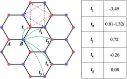
Figure 1: Left panel: Schematic illustration of Kane-Mele model on honeycomb lattice. $t_{n}$ is the hopping parameter. The next-nearest neighbor hoppings have a sublattice, spin, and direction-dependent phase factors, as illustrated by the dashed arrows. Right panel: Numerical values of $t_{n}$ in unit of meV at $\theta=3.5^{\circ}$.

II.2 Mean-field calculation

We theoretically calculate the interaction-driven QAHI state in $t$MoTe₂ at hole filling factor $\nu=1$, which has been experimentally realized[75, 15, 16, 17, 18]. In our calculation, we use a band-projected interacting Hamiltonian $\hat{\mathcal{H}}$ by retaining the top two moiré valence bands in $t$MoTe₂, which includes both the single-particle term $\hat{\mathcal{H}}_{\mathrm{KM}}$ of Eq. (3) and the Coulomb interaction term $\hat{\mathcal{H}}_{\text{int}}$ as follows,

$$\hat{\mathcal{H}}_{\textrm{int}}=\frac{1}{2}\sum V_{\bm{k}_{1}\bm{k}_{2}\bm{k}_{3}\bm{k}_{4}}^{n_{1}n_{2}n_{3}n_{4}}\left(\tau,\tau^{\prime}\right)b_{\bm{k}_{1}n_{1}\tau}^{\dagger}b_{\bm{k}_{2}n_{2}\tau^{\prime}}^{\dagger}b_{\bm{k}_{3}n_{3}\tau^{\prime}}b_{\bm{k}_{4}n_{4}\tau},$$ (4)

where $V_{\bm{k}_{1}\bm{k}_{2}\bm{k}_{3}\bm{k}_{4}}^{n_{1}n_{2}n_{3}n_{4}}\left(\tau,\tau^{\prime}\right)$ is the Coulomb potential $V_{\bm{q}}=2\pi e^{2}\tanh{(|\bm{q}|d)}/(\epsilon|\bm{q}|)$ projected onto the moiré bands, where $d$ is the gate-to-sample distance and $\epsilon$ is the dielectric constant. In our calculation, we set $d=20$ nm, $\epsilon=15$. The details on the construction of $\hat{\mathcal{H}}_{\textrm{int}}$ can be found in Ref. [58].

We perform mean-field studies of $\hat{\mathcal{H}}$ using self-consistent HF approximation at $\nu=1$ to obtain the QAHI state valley (spin) polarization. The mean-field Hamiltonian for the QAHIs phase can be formally written as

$$\hat{\mathcal{H}}_{\text{MF}}=\sum_{\boldsymbol{k},\tau,\lambda}E_{\bm{k}}^{\lambda\tau}f_{\boldsymbol{k}\lambda\tau}^{\dagger}f_{\boldsymbol{k}\lambda\tau},$$ (5)

where $E_{\bm{k}}^{\lambda\tau}$ and $\lambda$ are, respectively, the energy and band index for the interaction renormalized band structure. Here $f_{\boldsymbol{k}\lambda\tau}^{\dagger}$ and $b_{\boldsymbol{k}n\tau}^{\dagger}$ operators are related by unitary transformations determined by the HF calculation. In Fig. 2(a), we show the mean-field band structure for the QAHI state at $\theta=3.5^{\circ}$. The occupied band with a Chern number $C$ of $|C|=1$ is valley polarized and separated by a mean-field energy gap of 32 meV from unoccupied bands. The spontaneous valley polarization in the QAHI state spontaneously breaks the time-reversal symmetry $\hat{\mathcal{T}}$, but does not break the continuous valley $U(1)$ symmetry. For definiteness, the QAHI state is assumed to be polarized to the $\tau=+$ valley unless otherwise specified.

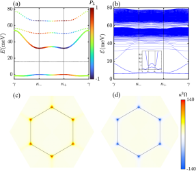
Figure 2: (a) HF band structure of the QAHI at $\theta=3.5^{\circ}$ in the hole basis. The solid (dashed) lines plot bands in $\tau=+(-)$ valley. The dotted horizontal line marks the middle of the gap. The color represents the layer polarization $P_{L}$ with $+1$ $(-1)$ indicating the bottom (top) layer. (b) Magnon spectrum calculated for the $\nu=1$ QAHI state at $\theta=3.5^{\circ}$. The inset is a zoom-in plot. (c),(d) The Berry curvature $\Omega$ for the first and second band in (b). $\kappa$ is $4\pi/3a_{M}$. The black hexagon in (c) and (d) marks the mBZ.

III Topological magnons

III.1 Magnon spectrum

Based on the QAHI state in Fig. 2 (a), we study intervalley collective excitations where the particle is excited from the occupied band at $\tau=+$ to the unoccupied bands at $\tau=-$. This excitation carries a single spin flip due to spin-valley locking and therefore, is equivalent to magnon. The collective magnon excitations can be parametrized as [76]

$$|\chi,\bm{q}\rangle=\sum_{\bm{k},\lambda}z_{\bm{k}}^{\lambda}(\chi,\bm{q})f_{\bm{k}+\bm{q},\lambda,-}^{\dagger}f_{\bm{k},1,+}|G\rangle,$$ (6)

where $|G\rangle$ is the Slate-determinant ground state obtained in the HF approximation, $\bm{q}$ is the center-of-mass (CM) momentum of the magnon, and $\chi$ is an index that labels the magnon states at a given $\bm{q}$. The magnon state $|\chi,\bm{q}\rangle$ corresponds to a superposition of particle-hole pairs $f_{\bm{k}+\bm{q},\lambda,-}^{\dagger}f_{\bm{k},1,+}|G\rangle$ with the envelop function $z_{\bm{k}}^{\lambda}(\chi,\bm{q})$, which satisfies the normalization condition $\sum_{\bm{k},\lambda}|z_{\bm{k}}^{\lambda}(\chi,\bm{q})|^{2}=1$. Variation of the energy $\langle\chi,\bm{q}|\hat{\mathcal{H}}|\chi,\bm{q}\rangle$ with respect to the parameter $z_{\bm{k}}^{\lambda}(\chi,\bm{q})$ leads to the Bethe-Salpeter equation,

$$\mathcal{E}_{\chi,\bm{q}}z_{\bm{k}}^{\lambda}(\chi,\bm{q})=\sum_{\bm{p}\lambda^{\prime}}\mathcal{H}^{\lambda\lambda^{\prime}}_{\bm{k}\bm{p}}(\bm{q})z_{\bm{p}}^{\lambda^{\prime}}(\chi,\bm{q}),$$ (7)

$$\mathcal{H}^{\lambda\lambda^{\prime}}_{\bm{k}\bm{p}}(\bm{q})=(E_{\bm{k}+\bm{q}}^{\lambda-}-E_{\bm{k}}^{1+})\delta_{\bm{k}\bm{p}}\delta_{\lambda\lambda^{\prime}}-\tilde{V}^{1\lambda\lambda^{\prime}1}_{\bm{p},\bm{k}+\bm{q},\bm{p}+\bm{q},\bm{k}}(+,-),$$

where $\mathcal{H}^{\lambda\lambda^{\prime}}_{\bm{k}\bm{p}}(\bm{q})$ includes the quasiparticle energy cost of particle-hole transition as well as electron-hole attractive interaction. Here $\tilde{V}$ denotes Coulomb matrix element in the basis of $f_{\boldsymbol{k}\lambda\tau}^{\dagger}$ operators. The study of intravalley exctions (i.e., intravalley collective excitations) in $t$MoTe₂ can be found in Ref. [47].

We obtain the magnon energy $\mathcal{E}_{\chi,\bm{q}}$ and wave function $|\chi,\bm{q}\rangle$ at each $\bm{q}$ by numerically diagonalizing the matrix $\mathcal{H}^{\lambda\lambda^{\prime}}_{\bm{k}\bm{p}}(\bm{q})$. The calculated magnon spectrum for the QAHIs phase at $\theta=3.5^{\circ}$ is shown in Fig. 2(b) and has the following important features. (1) All the magnon excitations have finite energies with a minimum of 6.4 meV. This is consistent with the fact that the QAHI state does not break any continuous symmetry, and therefore, there is no gapless Goldstone mode. The positive definiteness of the magnon excitation indicates the robustness of the QAHI state. (2) The lowest two magnon bands are isolated in energy from the continuous spectrum. (3) There is a small gap of value 0.2 meV that separates the lowest two magnon bands at the mBZ corners $\bm{\kappa}_{\pm}$. [See the inset of Fig. 2(b)]. We mainly focus on the first two magnon bands in the following.

We further calculate the Berry curvatures $\Omega$ and Chern numbers $C$ of the first two magnon bands using the method of Ref. [33] (See also Appendix A for details). The Berry curvatures $\Omega$, as shown in Figs. 2(c) and (d), are peaked at $\bm{\kappa}_{\pm}$ where the small gap is opened up and have opposite values for the first two magnon bands. The Chern numbers $C$, obtained from the integration of the Berry curvatures, are $-1$ and $+1$ for the first and second magnon bands, respectively. Therefore, the lowest two magnon bands are topological as characterized by the Chern numbers.

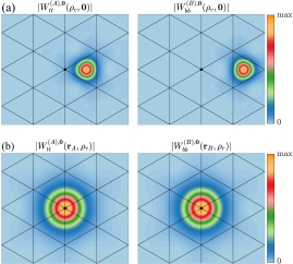
Figure 3: The amplitude of magnon Wannier states for $\theta=3.5^{\circ}$ at $\nu=1$. (a) $|W^{(A),\bm{0}}_{tt}(\bm{\rho}_{c},\bm{\rho}_{r})|$ and $|W^{(B),\bm{0}}_{bb}(\bm{\rho}_{c},\bm{\rho}_{r})|$ plotted in coordinate of $\bm{\rho}_{c}$ with $\bm{\rho}_{r}$ fixed at zero. (b) $|W^{(A),\bm{0}}_{tt}(\bm{\rho}_{c},\bm{\rho}_{r})|$ and $|W^{(B),\bm{0}}_{bb}(\bm{\rho}_{c},\bm{\rho}_{r})|$ plotted in coordinate of $\bm{\rho}_{r}$ with $\bm{\rho}_{c}$ fixed at $A$ and $B$ site, respectively. The black lines mark a triangular lattice with period $a_{M}$, and the black dot is the origin of the coordinates.

III.2 Magnon tight-binding model

To gain a deeper insight, we construct a tight-binding model based on magnon Wannier states for the first two magnon bands, which is feasible as their total Chern number is zero. We start by defining the real-space magnon Bloch wavefunction for the $|\chi,\bm{q}\rangle$ state as

$$g_{ll^{\prime}}^{\chi,\bm{q}}(\bm{r},\bm{r}^{\prime})=\sum_{\bm{k},\lambda}z^{\lambda}_{\bm{k}}(\chi,\bm{q})\psi^{\lambda}_{\bm{k}+\bm{q},l,-}(\bm{r})[\psi^{1}_{\bm{k},l^{\prime},+}(\bm{r}^{\prime})]^{*},$$ (8)

where $\bm{r}$ ($\bm{r}^{\prime}$) is the in-plane position of the $p^{*}$ ($h^{*}$) particle, and $l$ ($l^{\prime}$) is the corresponding layer index. Here $p^{*}$ ($h^{*}$) labels the particle (hole) in the hole basis that we employ. $\psi^{\lambda}_{\bm{k}+\bm{q},l,-}(\bm{r})$ [$\psi^{1}_{\bm{k},l^{\prime},+}(\bm{r}^{\prime})$] is the quasiparticle Bloch wavefunction at valley $\tau=-(+)$ obtained by the mean-field calculation. In contrast to the electron Bloch wavefunction, the magnon Bloch state describes a two-particle state with two coordinates $\bm{r}$ and $\bm{r}^{\prime}$. For convenience, we also define the CM coordinate $\bm{\rho}_{c}=(\bm{r}+\bm{r}^{\prime})/2$ and the relative coordinate $\bm{\rho}_{r}=\bm{r}-\bm{r}^{\prime}$.

To capture the first two magnon bands, we need two magnon Wannier states, which can be formally constructed as [77, 78],

$$W_{ll^{\prime}}^{(\alpha),\bm{R}}(\bm{\rho}_{c},\bm{\rho}_{r})=\frac{1}{\sqrt{N_{\bm{q}}}}\sum_{\bm{q}}e^{i\bm{q}\bm{R}}W_{ll^{\prime}}^{(\alpha),\bm{q}}(\bm{\rho}_{c},\bm{\rho}_{r}),$$ (9)

$$W_{ll^{\prime}}^{(\alpha),\bm{q}}(\bm{\rho}_{c},\bm{\rho}_{r})=\sum_{\chi=1,2}C^{(\alpha)}_{\chi,\bm{q}}g_{ll^{\prime}}^{\chi,\bm{q}}(\bm{\rho}_{c}+\frac{\bm{\rho}_{r}}{2},\bm{\rho}_{c}-\frac{\bm{\rho}_{r}}{2}).$$ (10)

In Eq. (9), $W^{(\alpha),\bm{R}}(\bm{\rho}_{c},\bm{\rho}_{r})$ is the magnon Wannier state with the CM wavefunction localized in the moiré unit cell $\bm{R}$, $W^{(\alpha),\bm{q}}(\bm{\rho}_{c},\bm{\rho}_{r})$ is the corresponding Bloch-like state derived from the Wannier state, and $N_{\bm{q}}$ is the number of $\bm{q}$ points included in the summation. The index $\alpha$ labels the two magnon Wannier states, and we use the $A$ and $B$ symbols for the two values of $\alpha$ with reasons to be clear shortly. In Eq. (10), the Bloch-like state $W^{(\alpha),\bm{q}}(\bm{\rho}_{c},\bm{\rho}_{r})$ is obtained by a unitary transformation from the magnon Bloch wavefunctions, where the coefficients $C^{(\alpha)}_{\chi,\bm{q}}$ form a unitary matrix $U(\bm{q})$ at each $\bm{q}$,

$$U(\bm{q})=\left[\begin{array}[]{cc}C^{(A)}_{1,\bm{q}}&C^{(B)}_{1,\bm{q}}\\ C^{(A)}_{2,\bm{q}}&C^{(B)}_{2,\bm{q}}\\ \end{array}\right].$$ (11)

We now provide a procedure to determine the unitary matrix $U(\bm{q})$. Since the fermionic model in Eq. (2) is based on a honeycomb lattice formed by $A$ and $B$ sites, we can take an ansatz that the CM wavefunction of the magnon Wannier state $W^{(\alpha),\bm{R}}(\bm{\rho}_{c},\bm{\rho}_{r})$ is centered at the $\alpha$ site for $\alpha=A,B$. For this purpose, we define the following sublattice polarization function,

$$F^{(\alpha)}_{\bm{q}}=|W_{tt}^{(\alpha),\bm{q}}(\bm{r}_{A},\bm{0})|^{2}-|W_{bb}^{(\alpha),\bm{q}}(\bm{r}_{B},\bm{0})|^{2},$$ (12)

where $\bm{r}_{A}=(a_{M}/\sqrt{3},0)$ and $\bm{r}_{B}=(2a_{M}/{\sqrt{3}},0)$ are, respectively, the positions of $A$ and $B$ sites at the $\bm{R}=\bm{0}$ unit cell. Under the normalization constraint of $\sum_{\chi=1,2}|C^{(\alpha)}_{\chi,\bm{q}}|^{2}=1$, we obtain $C^{(\alpha)}_{\chi,\bm{q}}$ by maximizing (minimizing) the function $F^{(\alpha)}_{\bm{q}}$ for $\alpha=A(B)$. This procedure automatically leads to a unitary matrix $U(\bm{q})$. We further fix the gauge by requiring that $W_{tt}^{(A),\bm{q}}(\bm{r}_{A},\bm{0})>0$ and $W_{bb}^{(B),\bm{q}}(\bm{r}_{B},\bm{0})>0$. Here we employ the locking between site and layer, as the $A$ ($B$) site is polarized to the $t$ ($b$) layer.

The constructed $W^{(\alpha),\bm{R}}(\bm{\rho}_{c},\bm{\rho}_{r})$ using the above method are shown in Fig. 3 for $\bm{R}=\bm{0}$ and $\theta=3.5^{\circ}$, which plots the amplitude with fixed $\bm{\rho}_{r}$ in Fig. 3(a) and fixed $\bm{\rho}_{c}$ in Fig. 3(b), respectively. Here, we only show $W_{tt}^{(A),\bm{0}}(\bm{\rho}_{c},\bm{\rho}_{r})$ and $W_{bb}^{(B),\bm{0}}(\bm{\rho}_{c},\bm{\rho}_{r})$ since the two magnon Wannier states are mostly distributed at $l=l^{\prime}=t$ and $l=l^{\prime}=b$, respectively. Consistent with the initial ansatz, the CM wavefunction of $W^{(\alpha),\bm{R}}(\bm{\rho}_{c},\bm{\rho}_{r})$ are indeed centered at the $\alpha$ site. Meanwhile, the relative motion wavefunction of $W^{(\alpha),\bm{R}}(\bm{\rho}_{c},\bm{\rho}_{r})$, as shown in Fig. 3(b), is $s$-wave like, which demonstrates the particle-hole bound state in the magnon. Overall, the magnon Wannier states capture the local spin flip at sites $A$ and $B$.

A tight-binding Hamiltonian can be constructed for the magnons based on the Wannier states,

$$\begin{split}H_{\text{mag}}&=\sum_{\alpha\beta}\sum_{\bm{R}\bm{R}^{\prime}}T_{\alpha\beta}(\bm{R}^{\prime}-\bm{R})a^{\dagger}_{\bm{R}\alpha}a_{\bm{R}^{\prime}\beta},\\ T_{\alpha\beta}(\bm{R})&=\frac{1}{N_{\bm{q}}}\sum_{\bm{q}\chi}e^{i\bm{q}\bm{R}}U^{\dagger}_{\alpha\chi}(\bm{q})\mathcal{E}_{\chi,\bm{q}}U_{\chi\beta}(\bm{q}),\end{split}$$ (13)

where $a^{\dagger}_{\bm{R}\alpha}$ ($a_{\bm{R}^{\prime}\beta}$) is the magnon creation (annihilation) operator at site $\alpha$ ($\beta$), $\mathcal{E}_{\chi,\bm{q}}$ is the magnon energy obtained from Eq. (7), and $U(\bm{q})$ is the unitary matrix defined in Eq. (11).

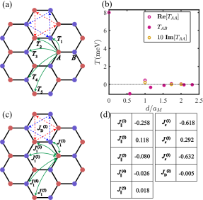
Figure 4: (a) Illustration of hopping parameters in the magnon tight-binding model. The next-nearest neighbor hoppings have a sublattice and direction-dependent phase factors, as illustrated by the dashed arrows. (b) Numerical values of hopping terms in the magnon tight-binding model as a function of two-site distance $d$. (c) Illustration of the effective spin model on the honeycomb lattice. The dashed arrows indicate the DMI between the next-nearest neighbors. (d) Numerical values of spin coupling constants in the unit of meV at $\theta=3.5^{\circ}$.

In Fig. 4(b), we plot $T_{\alpha\beta}(\bm{R})$ as a function of the hopping distance $d=|\bm{R}+\bm{r}_{\beta}-\bm{r}_{\alpha}|$, where the hopping $T_{\alpha\beta}(\bm{R})$ decreases exponentially with $d$ for large $d$ [77]. Notably, the next-nearest neighbor hopping terms are complex with sublattice and direction-dependent phase factors $e^{i\phi_{T}\nu_{ij}}$, where $\phi_{T}$ is a phase and $\nu_{ij}=+1(-1)$ if the hopping from the site $i$ to $j$ is along (against) the dashed arrows in Fig. 4(a). Therefore, Eq. (13) realizes an effective Haldane model for magnons [79, 80], where the complex next-nearest neighbor hopping terms induces topological gap at $\bm{\kappa}_{\pm}$, endowing the two magnon bands with opposite Chern numbers. We emphasize that the onsite energy $T_{\alpha\alpha}(\bm{0})\approx 8$ meV is an important term, as the magnon energy is already defined relative to the ground state.

IV Domain walls

We now study another type of excited state, i.e., domain walls that separate real-space regions with opposite valley (spin) polarizations. We study a domain structure shown in Fig. 5(b), where the valley polarizations change signs twice along the $\hat{\bm{e}}_{1}=(\sqrt{3}/2,1/2)$ direction, leading to two parallel domain walls along the $\hat{\bm{e}}_{2}=(0,1)$ direction. We apply periodic boundaries for the superstructure with a length $L_{i}=N_{i}a_{M}$ along the $\hat{\bm{e}}_{i}$ direction for $i=1,2$. We note that the superstructure has a period of $L_{1}$ along the $\hat{\bm{e}}_{1}$ direction due to the presence of the domains, but $a_{M}$ along the $\hat{\bm{e}}_{2}$ direction. Therefore, the Brillouin zone for the superstructure (see inset of Fig. 5(a) for illustration), denoted as bz for shorthand notation, is reduced compared to the mBZ.

We perform self-consistent HF calculation for the superstructure with two domain walls by sampling the bz using a centered scheme with a $1\times N_{2}$ $k$-point mesh, where $N_{2}$ is taken to be 15. In the iterative HF calculation, we start with a configuration with two domain walls, which remain after the self-consistent calculation. In the iteration, the filling factor is fixed at $\nu=1$. The resulting mean-field band structure is shown in Fig. 5(a) for a superstructure with $L_{1}=14a_{M}$. Since each domain wall separates Chern insulators with opposite valley polarization and therefore, opposite Chern numbers, it binds chiral electronic edge states within the bulk insulating gap. Because the change of Chern numbers across each domain wall is 2, there are two chiral electronic edge states per domain wall. Moreover, the left and right domain walls host chiral edge states with opposite velocities. All these expected features are indeed obtained from our calculation, as shown by the energy spectrum in Fig. 5(a) and the chiral state wavefunctions in Fig. 5(b). We view these domain walls as topological, as they host the chiral states.

The domain walls are excited states and cost a finite energy compared to the ground state. We denote the energy cost of a domain wall per unit cell along the $\hat{\bm{e}}_{2}$ direction as $\mathcal{E}_{\text{DW}}$. Here $\mathcal{E}_{\text{DW}}=(E_{2}-E_{0})/(2N_{2})$, where $E_{2}$ and $E_{0}$ are respectively the total energy of the $L_{1}\times L_{2}$ superstructure with two and no domain walls. In Fig. 5(c), we plot $\mathcal{E}_{\text{DW}}$ as a function of $L_{1}$. The convergence of $\mathcal{E}_{\text{DW}}\approx 2.69$ meV is achieved for $L_{1}=14a_{M}$, above which the interactions between the two domain walls separated by a length of $L_{1}/2$ is negligible.

Figure 5: (a) HF band structure of the domain structure shown in (b) with $L_{1}=14a_{M}$, where the valley polarizations change signs twice along the $\hat{\bm{e}}_{1}=(\sqrt{3}/2,1/2)$ direction. The inset shows the Brillouin zone (bz) of the domain superstructure. The gray bands belong to the bulk states. Red (blue) colors are used to distinguish in-gap chiral states localized at the left (right) domain wall. The horizontal dotted line marks the middle of the insulating gap of the uniform QAHI at $\nu=1$. (b) The wavefunction amplitude of chiral edge states labeled on the spectrum in (a). (c) The domain wall energy as a function of $L_{1}$. These results are calculated at $\theta=3.5^{\circ}$.

V Effective spin model

We propose an effective spin model to provide a unified low-energy description of the magnon and domain wall excitations. The construction of this effective model is informed by the following properties of the system. (1) The ground state is a ferromagnetic state with aligned out-of-plane spin polarizations on a honeycomb lattice. (2) The two low-energy magnon bands are derived from spin flips on the $A$ and $B$ sublattices of the honeycomb lattice. (3) The system hosts Ising-type domain walls. We use the following nonlinear sigma model defined on a honeycomb lattice for the effective spin model, with the Lagrangian given by,

$$\begin{split}\mathcal{L}_{S}&=\mathcal{B}_{S}-\mathcal{E}[\bm{m}],\\ \mathcal{B}_{S}&=-\frac{\hbar}{2}\sum_{\bm{R}\alpha}n_{\alpha}\mathcal{\bm{A}}[\bm{m}_{\bm{R}\alpha}]\cdot\partial_{t}\bm{m}_{\bm{R}\alpha},\\ \mathcal{E}[\bm{m}]&=\sum^{\prime}_{\bm{R}\bm{R}^{\prime}\alpha\beta}\sum_{i}J^{\alpha\beta}_{i}(\bm{R}^{\prime}-\bm{R})m^{i}_{\bm{R}\alpha}m^{i}_{\bm{R}^{\prime}\beta}\\ &+\sum^{\prime}_{\bm{R}\bm{R}^{\prime}\alpha}J^{\alpha\alpha}_{D}(\bm{R}^{\prime}-\bm{R})(\bm{m}_{\bm{R}\alpha}\times\bm{m}_{\bm{R}^{\prime}\alpha})\cdot\hat{z},\end{split}$$ (14)

where $\bm{m}_{\bm{R}\alpha}=(m^{x}_{\bm{R}\alpha},m^{y}_{\bm{R}\alpha},m^{z}_{\bm{R}\alpha})$ is a unit vector that describes the magnetization direction at sublattice $\alpha$ and unit cell $\bm{R}$ of a honeycomb lattice. Here $\mathcal{B}_{S}$ is the kinetic Berry phase, where $\mathcal{\bm{A}}[\bm{m}_{\bm{R}\alpha}]$ is the effective spin gauge field defined by $\bm{\nabla}_{\bm{m}}\times\mathcal{\bm{A}}[\bm{m}]=\bm{m}$, $n_{\alpha}$ is the average occupation number at the sublattice $\alpha$, and $\partial_{t}$ is the derivative with respect to time $t$. At $\nu=1$, $n_{\alpha}$ is $1/2$. The energy functional $\mathcal{E}[\bm{m}]$ is expressed by the classical spin couplings on the honeycomb lattice, of which the form is constrained by the symmetry of the system, in particular the $\hat{D}_{3d}$ point group symmetry and the spin $U(1)$ symmetry. The first line in the expression of $\mathcal{E}[\bm{m}]$ describes the spin couplings in the XXZ Heisenberg model, where the in-plane coupling constant satisfies $J^{\alpha\beta}_{x}(\bm{R})=J^{\alpha\beta}_{y}(\bm{R})=J^{\alpha\beta}_{\|}(\bm{R})$ due to the spin $U(1)$ symmetry and $J^{\alpha\beta}_{z}(\bm{R})$ is the out-of-plane coupling constant. The second line in $\mathcal{E}[\bm{m}]$ is the DMI between spins on next-nearest neighbors, with the direction from site $\bm{R}\alpha$ to $\bm{R}^{\prime}\alpha$ specified by the dashed arrows in Fig. 4(c). The prime in the summations denotes that each bond is counted only once. The form of $\mathcal{L}_{S}$ in Eq. (14) is justified by a microscopic derivation presented in Appendix B.

The coupling constants $\{J_{\|},J_{z},J_{D}\}$ of the above effective model can be extracted from the numerical results of magnons in Sec. III and domain walls in Sec. IV. We first consider magnon excitations by taking the in-plane components $\{m^{x}_{\bm{R}\alpha},m^{y}_{\bm{R}\alpha}\}$ as small fluctuations. With the approximation of $m^{z}_{\bm{R}\alpha}\approx 1-\frac{1}{2}[(m^{x}_{\bm{R}\alpha})^{2}+(m^{y}_{\bm{R}\alpha})^{2}]$, the energy functional $\mathcal{E}[\bm{m}]$ is expanded to second order in $\{m^{x}_{\bm{R}\alpha},m^{y}_{\bm{R}\alpha}\}$, while the kinetic Berry phase can be expressed as,

$$\begin{split}\mathcal{B}_{S}&=-\frac{\hbar}{4}\sum_{\alpha}\sum_{\bm{R}}n_{\alpha}(m^{x}_{\bm{R}{\alpha}}\partial_{t}m^{y}_{\bm{R}{\alpha}}-m^{y}_{\bm{R}{\alpha}}\partial_{t}m^{x}_{\bm{R}{\alpha}}),\end{split}$$ (15)

We derive the equation of motion for $m^{+}_{\bm{R}{\alpha}}=m^{x}_{\bm{R}{\alpha}}+im^{y}_{\bm{R}{\alpha}}$ using the Lagrangian $\mathcal{L}_{S}$ and compare it with that for the magnon annihilation operator $a_{\bm{R}{\alpha}}$ using the magnon tight-binding Hamiltonian in Eq. (13). The comparison is motivated by the Holstein–Primakoff transformation that maps the spin operators to boson operators and relates the spin coupling constants with the hopping parameters in Eq. (13),

$$\sum_{\bm{R}\beta}J^{\alpha\beta}_{z}(\bm{R})=-\frac{1}{4}T_{\alpha\alpha}(\bm{0}),$$ (16)

$$J^{\alpha\beta}_{\|}(\bm{R})=\frac{1}{4}\text{Re}[T_{\alpha\beta}(\bm{R})],$$ (17)

$$J^{\alpha\alpha}_{D}(\bm{R})=-\frac{1}{4}\text{Im}[T_{\alpha\alpha}(\bm{R})].$$ (18)

This set of equations shows that coupling constants $J_{\|}$ and $J_{D}$ are directly determined by the hopping parameters, while only a sum rule is obtained for the out-of-plane coupling constants $J_{z}$. Equation (18) demonstrates that the DMI coupling constant $J^{\alpha\alpha}_{D}(\bm{R})$ is proportional to $\text{Im}[T_{\alpha\alpha}(\bm{R})]$. Since $\text{Im}[T_{\alpha\alpha}(\bm{R})]$ is finite only for next-nearest neighbors as shown in Fig. 4(a), we only keep the DMI terms between next-nearest neighbors in the effective spin model, which results in the topological gap between the magnon bands. We list numerical values of $J_{\|}$ and $J_{D}$ in Fig. 4(d). The in-plane coupling constants between the nearest neighbors, second and third are, respectively, $J_{\|}^{(1)}=-0.258$ meV, $J_{\|}^{(2)}=0.118$ meV, and $J_{\|}^{(3)}=-0.08$ meV. For comparison, the DMI coupling constant between the second-nearest neighbors is $J_{D}^{(2)}=-0.005$ meV, which is orders of magnitude smaller than the corresponding $J_{\|}^{(2)}$.

To further determine the value of each $J^{\alpha\beta}_{z}(\bm{R})$, we turn to the domain wall excitation. We consider a domain wall along the $\hat{\bm{e}}_{2}$ direction that separates two regions with opposite out-of-plane magnetization, i.e., $m_{\bm{R}\alpha}^{z}=-1$ and $m_{\bm{R}^{\prime}\alpha^{\prime}}^{z}=+1$, where $\bm{R}\alpha$ ($\bm{R}^{\prime}\alpha^{\prime}$) are sites on the left (right) hand side of the domain wall. The energy cost per unit cell along $\hat{\bm{e}}_{2}$ of the domain wall compared to the ferromagnetic ground state is

$$\begin{split}\mathcal{E}_{\text{DW}}=-2J^{(1)}_{z}-8J^{(2)}_{z}-6J^{(3)}_{z}.\end{split}$$ (19)

Here $J^{\alpha\beta}_{z}(\bm{R})$ is written as the $n$th nearest-neighbor terms $J^{(n)}_{z}$, which are truncated up to $n=3$. From the numerical calculation presented in Sec. IV, we have $\mathcal{E}_{\text{DW}}\approx 2.69$ meV. In addition to Eqs. (16) and  (19), another equation can be derived by comparing the energy difference per unit cell between an out-of-plane antiferromagnetic (AF_z) state and the ferromagnetic QAHI ground state as,

$$\begin{split}E_{\text{AF}_{z}}-E_{\text{QAHI}}=-6J^{(1)}_{z}-6J^{(3)}_{z}.\end{split}$$ (20)

Here the AF_z state has opposite out-of-plane spin polarizations on the $A$ and $B$ sublattices and is a meta-stable state that can be obtained within the self-consistent HF calculation, which leads to $E_{\text{AF}_{z}}-E_{\text{QAHIs}}=7.5$ meV. By combining Eqs. (16),  (19) and  (20), we obtain the three out-of-plane coupling constants $[J^{(1)}_{z},J^{(2)}_{z},J^{(3)}_{z}]=(-0.62,0.29,-0.63)$ meV. Here $J^{(1)}_{z}$ is negative, indicating the ferromagnetic coupling nature between the nearest neighbors on the honeycomb lattice. The magnitude of $J^{(n)}_{z}$ is larger than that of $J^{(n)}_{\|}$, which is a manifestation of the Ising anisotropy.

The effective spin model in Eq. (14) is now fully determined with the coupling constants obtained from microscopic calculations. This effective model gives rise to the correct out-of-plane ferromagnetic ground state, and quantitatively reproduces the topological magnon spectrum and the energy cost of domain wall excitations.

We can estimate the magnetic ordering temperature for the ferromagnetic ground state based on the effective spin model. By using the Ising mean-field theory on a honeycomb lattice, where the in-plane spin fluctuation is ignored, the magnetic ordering temperature $T_{c}$ can be approximated as,

$$T_{c}\approx-\frac{\sum_{\bm{R}\beta}J^{\alpha\beta}_{z}(\bm{R})}{k_{B}}=\frac{T_{\alpha\alpha}(\bm{0})}{4k_{B}}\approx 23~\text{K},$$ (21)

where $k_{B}$ is the Boltzmann constant. Here the value of $T_{c}\approx 23~\text{K}$ is a mean-field estimation that serves as an upper limit of the ferromagnetic Curie temperature. Experimentally, the Curie temperature for the QAHI state in $t$MoTe₂ with $\theta$ around $3.5^{\circ}$ is about 12 K  [75, 15, 18]. Our mean-field estimation of $T_{c}$ is qualitatively consistent with this experimental value. We note that our estimation does not take into account the disorder effect, which can reduce the experimental $T_{c}$.

VI discussion and summary

In summary, we present a theoretical study of magnon and domain wall excitations for the QAHI state in twisted bilayer $t$MoTe₂ at $\nu=1$. Our numerical calculation starts from a generalized interacting Kane-Mele model projected onto the first two moiré bands. Based on the mean-field QAHI ground state and the Bethe-Salpeter equation, we obtain the magnon spectrum, where the first two bands have opposite Chern numbers. An effective Haldane model is constructed to characterize the two magnon bands. We further study a structure of domain walls that separate regions with opposite valley polarization and Chern numbers. The energy cost of the domain wall is calculated. The above two magnetic excitations are phenomenologically described by an effective spin model, which consists of in-plane and out-of-plane Heisenberg spin coupling, as well as the DMI terms between next-nearest neighbors on the honeycomb lattice. The DMI terms are crucial to account for the magnon topology. The values of coupling constants in the effective spin model are determined from the numerical results for magnons and domain walls. The estimation of magnetic ordering temperature $T_{c}$ based on the spin coupling constants is qualitatively consistent with the experimental value. We note that the $k_{B}T_{c}\approx 2$ meV estimated from the effective spin model is an order of magnitude smaller than the charge gap $(\sim 32~\text{meV})$ obtained from the HF band structure [Fig. 2(a)], and also a few times smaller than the minimum magnon excitation energy $(\sim 6.4~\text{meV})$ [Fig. 2(b)]. This indicates that the domain-wall thermal proliferation limits the Curie temperature.

The QAHI ground state does not allow the description in terms of the occupation of a set of exponentially localized orbitals on a periodic lattice due to Wannier obstruction. Nevertheless, we show that low-energy magnon bands on top of the QAHI ground state can have a tight-binding model description based on localized magnon Wannier states. It should be noted that the magnons are two-particle bound states of electron and hole, which involves both occupied and unoccupied states. Given the Wannier obstruction of the QAHI ground state, we propose using the Lagrangian in Eq. (14) to describe the effective spin model, which incorporates the fact that the average fermion occupation number per site is fractional rather than an integer. This contrasts with the effective spin Hamiltonian of a Mott insulator, where electrons are localized at each site with integer occupation. Due to the magnon topology, we construct a lattice-based nonlinear sigma model instead of the conventional continuous nonlinear sigma model, which has been used to describe the long-wavelength behavior of collective excitations[81, 30, 37, 41, 49]. The continuous model discards lattice information, making it unsuitable for capturing the topology of collective excitations. In this regard, it would be interesting to revisit the collective excitations of interaction-driven symmetry-breaking insulating states in magic-angle twisted bilayer graphene and explore whether a lattice formulation of the nonlinear sigma model can be developed[82].

VII ACKNOWLEDGMENTS

We thank Xun-Jiang Luo for the valuable discussions. This work is supported by National Key Research and Development Program of China (Grants No. 2022YFA1402401 and No. 2021YFA1401300), National Natural Science Foundation of China (Grant No. 12274333 and No. 12404084). W.-X. Q. is also supported by the China Postdoctoral Science Foundation (Grants No. 2024T170675 and No. 2023M742716). The numerical calculations in this paper have been done on the supercomputing system in the Supercomputing Center of Wuhan University.

Note Added. As this manuscript was being prepared, we learned of a related study by W.-T. Zhou et al., which reaches consistent conclusions about the magnon topology in $t$MoTe₂.

Appendix A Calculation of magnon Chern number

In the presence of electron-hole interactions, the magnon states excited from $\tau=+$ to $\tau=-$ at $\nu=1$ can be parametrized as in Eq. (6), where $f_{\bm{k}+\bm{q},\lambda,-}^{\dagger}(f_{\bm{k},1,+})$ can be expanded by field operator at real space $\bm{r}$ in layer $\ell$ as

$$\begin{split}&f_{\bm{k}+\bm{q},\lambda,-}^{\dagger}=\sum_{\ell}\int d\bm{r}\psi^{\lambda}_{\bm{k}+\bm{q},\ell,-}(\bm{r})f_{\ell\bm{r}}^{\dagger},\\ &f_{\bm{k},1,+}=\sum_{\ell}\int d\bm{r}[\psi^{1}_{\bm{k},\ell,+}(\bm{r})]^{*}f_{\ell\bm{r}}.\end{split}$$ (22)

Then

$$|\chi,\bm{q}\rangle=\sum_{\ell,\ell^{\prime}}\int d\bm{r}\int d\bm{r}^{\prime}g_{\ell\ell^{\prime}}^{\chi\bm{q}}(\bm{r},\bm{r}^{\prime})f_{\ell\bm{r}}^{\dagger}f_{\ell^{\prime}\bm{r}^{\prime}}|G\rangle,$$ (23)

where $g_{\ell\ell^{\prime}}^{\chi\bm{q}}(\bm{r},\bm{r}^{\prime})$ is the real-space magnon Bloch wavefunction of Eq. (8). The periodic part of $g_{\ell\ell^{\prime}}^{\chi\bm{q}}(\bm{r},\bm{r}^{\prime})$ can be expressed as

$$u_{\ell\ell^{\prime}}^{\chi\bm{q}}(\bm{r},\bm{r}^{\prime})=e^{-i\bm{q}\frac{\bm{r}+\bm{r}^{\prime}}{2}}\sum_{\bm{k},\lambda}z^{\lambda}_{\bm{k}}(\chi,\bm{q})\psi^{\lambda}_{\bm{k}+\bm{q},\ell,-}(\bm{r})[\psi^{1}_{\bm{k},\ell^{\prime},+}(\bm{r}^{\prime})]^{*}.$$ (24)

We compute the overlap integral as,

$$\begin{split}\langle u^{\chi\bm{q}}|u^{\chi,\bm{q}+\bm{q}_{0}}\rangle&=\sum_{\bm{k}\bm{k}^{\prime}}\sum_{\lambda,\lambda^{\prime}}[z^{\lambda}_{\bm{k}}(\chi,\bm{q})]^{*}z^{\lambda^{\prime}}_{\bm{k}^{\prime}}(\chi,\bm{q}+\bm{q}_{0})\\ &\int{d\bm{r}}e^{-i\frac{\bm{q}_{0}}{2}\bm{r}}\sum_{\ell}[\psi^{\lambda}_{\bm{k}+\bm{q},\ell,-}(\bm{r})]^{*}\psi^{\lambda^{\prime}}_{\bm{k}^{\prime}+\bm{q}+\bm{q}_{0},\ell,-}(\bm{r})\\ &\int{d\bm{r}^{\prime}}e^{-i\frac{\bm{q}_{0}}{2}\bm{r}^{\prime}}\sum_{\ell^{\prime}}[\psi^{1}_{\bm{k}^{\prime},\ell^{\prime},+}(\bm{r}^{\prime})]^{*}\psi^{1}_{\bm{k},\ell^{\prime},+}(\bm{r}^{\prime})\\ &=\sum_{\bm{k}}\sum_{\lambda,\lambda^{\prime}}[z^{\lambda}_{\bm{k}}(\chi,\bm{q})]^{*}z^{\lambda^{\prime}}_{\bm{k}-\frac{\bm{q}_{0}}{2}}(\chi,\bm{q}+\bm{q}_{0})\\ &\langle u^{\lambda}_{\bm{k}+\bm{q},-}|u^{\lambda^{\prime}}_{\bm{k}+\bm{q}+\frac{\bm{q}_{0}}{2},-}\rangle\langle u^{1}_{\bm{k}-\frac{\bm{q}_{0}}{2},+}|u^{1}_{\bm{k},+}\rangle\end{split}$$ (25)

where $|u^{\lambda}_{\bm{k},\tau}\rangle$ is the periodic part of $\psi_{\bm{k},\tau}^{\lambda}$. The Berry curvature of $\chi$-th magnon band at each $\bm{q}$ can be calculated using Eq. (25) as follows,

$$\begin{split}\Omega_{\chi\bm{q}}=&\frac{1}{\delta\mathcal{A}_{0}}\text{Arg}[\langle u^{\chi\bm{q}}|u^{\chi,\bm{q}+\bm{q}_{1}}\rangle\langle u^{\chi,\bm{q}+\bm{q}_{1}}|u^{\chi,\bm{q}+\bm{q}_{1}+\bm{q}_{2}}\rangle\\ &\langle u^{\chi,\bm{q}+\bm{q}_{1}+\bm{q}_{2}}|u^{\chi,\bm{q}+\bm{q}_{2}}\rangle\langle u^{\chi,\bm{q}+\bm{q}_{2}}|u^{\chi\bm{q}}\rangle],\end{split}$$ (26)

where $\bm{q}$, $\bm{q}+\bm{q}_{1}$, $\bm{q}+\bm{q}_{1}+\bm{q}_{2}$, and $\bm{q}+\bm{q}_{2}$ are four corners of a small plaquette with an area $\delta\mathcal{A}_{0}$ in the momentum mesh. The Chern number for the $\chi$-th magnon band can be expressed as

$$\begin{split}C_{\chi}=\frac{1}{2\pi}\int_{mBZ}d\bm{q}\ \Omega_{\chi\bm{q}}.\end{split}$$ (27)

Appendix B Derivation of effective spin model

We present a microscopic derivation of the Lagrangian for the effective spin model in Eq. (14). To capture the main physics and make analytical progress, we consider a simplified Hamiltonian of Kane-Mele-Hubbard model, which only takes into account the onsite Hubbard interaction. This model can capture the essential physics of the QAHI state at $\nu=1$ and its collective excitation, as we show in the following.

The Kane-Mele-Hubbard model is given by,

$$\hat{\mathcal{H}}_{\mathrm{KMH}}=\hat{\mathcal{H}}_{\mathrm{KM}}+\hat{\mathcal{H}}_{U},$$ (28)

$$\hat{\mathcal{H}}_{\mathrm{KM}}=\sum_{\boldsymbol{k}}b_{\boldsymbol{k}}^{\dagger}\left[F_{\bm{k}}^{0}\sigma_{0}s_{0}+F_{\bm{k}}^{x}\sigma_{x}s_{0}+F_{\bm{k}}^{y}\sigma_{y}s_{0}+F_{\bm{k}}^{z}\sigma_{z}s_{z}\right]b_{\boldsymbol{k}},$$

$$\qquad\ =\sum_{\alpha\beta}\sum_{\bm{k}\tau}h^{\alpha\beta}_{\bm{k}\tau}b^{\dagger}_{\bm{k}\alpha\tau}b_{\bm{k}\beta\tau},$$

$$\hat{\mathcal{H}}_{U}=U\sum_{\alpha}\sum_{\bm{R}}\hat{n}_{\bm{R}\alpha\uparrow}\hat{n}_{\bm{R}\alpha\downarrow}$$

where $\hat{\mathcal{H}}_{\mathrm{KM}}$ is obtained by Fourier transformation form Eq. (2), and $b_{\boldsymbol{k}}=\{b_{\boldsymbol{k}A+},b_{\boldsymbol{k}A-},b_{\boldsymbol{k}B+},b_{\boldsymbol{k}B-}\}^{\mathrm{T}}$. Here $\sigma_{x,y,z}(\sigma_{0})$ and $s_{x,y,z}(s_{0})$ are, respectively, Pauli matrices (identity matrices) in the sublattice and spin spaces. $F^{0}_{\bm{k}}$ and $\bm{F}_{\bm{k}}=[F^{x}_{\bm{k}}\quad F^{y}_{\bm{k}}\quad F^{z}_{\bm{k}}]$ are real functions of the momentum $\boldsymbol{k}$. The $F^{z}_{\bm{k}}$ term characterizes the Ising spin-orbit coupling in the Kane-Mele model. Due to the time-reversal symmetry, $F_{\bm{k}}^{0}$ and $F_{\bm{k}}^{x}$ are even functions of $\bm{k}$, while $F_{\bm{k}}^{y}$ and $F_{\bm{k}}^{z}$ are odd functions of $\bm{k}$. We use $h_{\bm{k}\tau}$ to represent the $2\times 2$ single-particle Hamiltonian matrix for spin $\tau$. $\hat{\mathcal{H}}_{U}$ is the Hubbard term with onsite Coulomb repulsion $U$.

At $\nu=1$, the Kane-Mele-Hubbard model can support the QAHI state with full spin (valley) polarization for a sufficiently large Hubbard $U$ [26, 58]. We assume the QAHI state is polarized to valley $\tau=+$ (spin up), and the corresponding density matrix can be expressed as,

$$\langle b^{\dagger}_{\bm{k}A+}b_{\bm{k}A+}\rangle=\frac{1}{2}(1-\frac{F^{z}_{\bm{k}}}{|\bm{F}_{\bm{k}}|}),\ \langle b^{\dagger}_{\bm{k}A+}b_{\bm{k}B+}\rangle=-\frac{F^{x}_{\bm{k}}+iF^{y}_{\bm{k}}}{2|\bm{F}_{\bm{k}}|},$$ (29)

$$\langle b^{\dagger}_{\bm{k}B+}b_{\bm{k}A+}\rangle=-\frac{F^{x}_{\bm{k}}-iF^{y}_{\bm{k}}}{2|\bm{F}_{\bm{k}}|},\ \langle b^{\dagger}_{\bm{k}B+}b_{\bm{k}B+}\rangle=\frac{1}{2}(1+\frac{F^{z}_{\bm{k}}}{|\bm{F}_{\bm{k}}|}),$$

$$\langle b^{\dagger}_{\bm{k}\alpha-}b_{\bm{k}\beta-}\rangle=\langle b^{\dagger}_{\bm{k}\alpha+}b_{\bm{k}\beta-}\rangle=\langle b^{\dagger}_{\bm{k}\alpha-}b_{\bm{k}\beta+}\rangle=0,$$

where $|\bm{F}_{\bm{k}}|=\sqrt{(F_{\bm{k}}^{x})^{2}+(F_{\bm{k}}^{y})^{2}+(F_{\bm{k}}^{z})^{2}}$.

We now construct an effective theory based on the Hamiltonian in Eq. (28) and the following spin texture state [81]

$$\begin{split}|\bm{m}\rangle&=e^{-i\mathcal{F}}|\uparrow\rangle\approx(1-i\mathcal{F}-\frac{1}{2}\mathcal{F}^{2})|\uparrow\rangle,\\ \mathcal{F}&=\sum_{\bm{R}\alpha}(m^{x}_{\bm{R}\alpha}S^{y}_{\bm{R}\alpha}-m^{y}_{\bm{R}\alpha}S^{x}_{\bm{R}\alpha})\\ &=\sum_{\bm{q}\alpha}(m^{\alpha,x}_{-\bm{q}}S^{\alpha,y}_{\bm{q}}-m^{\alpha,y}_{-\bm{q}}S^{\alpha,x}_{\bm{q}}),\\ &\bm{S}_{\bm{R}\alpha}=\frac{1}{\sqrt{N}}\sum_{\bm{q}}e^{i\bm{q}\bm{R}}\bm{S}_{\bm{q}\alpha},\\ &\bm{S}_{\bm{q}\alpha}=\frac{1}{\sqrt{N}}\sum_{\bm{k}}\sum_{\tau_{1},\tau_{2}}b^{\dagger}_{\bm{k}+\bm{q},\alpha,\tau_{1}}\frac{\bm{s}_{\tau_{1},\tau_{2}}}{2}b_{\bm{k},\alpha,\tau_{2}},\end{split}$$ (30)

where $\bm{m}^{\alpha}_{\bm{q}}$ is the Fourier component of the unit vector $\bm{m}_{\bm{R}_{\alpha}}$ at sublattice $\alpha$ and unit cell $\bm{R}$, with small in-plane components $m^{x/y}_{\bm{R}\alpha}$, and $\bm{S}^{\alpha}_{\bm{q}}$ is the Fourier component of the local spin operator $\bm{S}_{\bm{R}\alpha}$. $\tau$ is the spin index. The operator $e^{-i\mathcal{F}}$ rotates the local spin direction from $\hat{z}$ to $\bm{m}_{\bm{R}\alpha}$. The corresponding state $|\bm{m}\rangle$ has a slowly varying spin texture relative to the QAHI ground state $|\uparrow\rangle$ at $\nu=1$ with spin up polarization, where the average occupation number at every sublattice is $n_{\alpha}=\frac{1}{2}$. By taking $m^{x/y}_{\bm{R}\alpha}$ as small parameters, the kinetic Berry phase $\mathcal{B}_{S}$ can be derived as

$$\begin{split}\mathcal{B}_{S}=&\langle\bm{m}|i\hbar\partial_{t}|\bm{m}\rangle\\ =&-\frac{\hbar}{4}\sum_{\alpha\bm{q}}n_{\alpha}(m^{\alpha,x}_{\bm{q}}\partial_{t}{m}^{\alpha,y}_{-\bm{q}}-m^{\alpha,y}_{\bm{q}}\partial_{t}{m}^{\alpha,x}_{-\bm{q}})\\ =&-\frac{\hbar}{4}\sum_{\alpha\bm{R}}n_{\alpha}(m^{x}_{\bm{R}\alpha}\partial_{t}{m}^{y}_{\bm{R}\alpha}-m^{y}_{\bm{R}\alpha}\partial_{t}{m}^{x}_{\bm{R}\alpha}),\end{split}$$ (31)

which justifies Eq. (15).

The energy of the spin texture state can be expanded in powers of $\mathcal{F}$ as,

$$\begin{split}\mathcal{E}[\bm{m}]=&\langle\bm{m}|\hat{\mathcal{H}}_{\mathrm{KMH}}|\bm{m}\rangle-\langle\hat{\mathcal{H}}_{\mathrm{KMH}}\rangle\\ \approx&i\langle[\mathcal{F},\hat{\mathcal{H}}_{\mathrm{KMH}}]\rangle-\frac{1}{2}\langle[\mathcal{F},[\mathcal{F},\hat{\mathcal{H}}_{\mathrm{KMH}}]]\rangle,\end{split}$$ (32)

where $\left\langle\cdots\right\rangle$ represents the ground state expectation value and the first term exactly vanishes. The second term can be divided into $\langle[\mathcal{F},[\mathcal{F},\mathcal{H}_{\mathrm{KM}}]]\rangle$ and $\langle[\mathcal{F},[\mathcal{F},\mathcal{H}_{U}]]\rangle$, where $\langle[\mathcal{F},[\mathcal{F},\mathcal{H}_{U}]]\rangle=0$ because $\mathcal{H}_{U}$ preserves spin SU(2) symmetry at each site. The nonzero term can be expressed as

$$\begin{split}\mathcal{E}[\bm{m}]=&-\frac{1}{2}\langle[\mathcal{F},[\mathcal{F},\hat{\mathcal{H}}_{\mathrm{KM}}]]\rangle\\ =&\sum_{\alpha}\sum_{\bm{q}}J^{\alpha\alpha}_{H}(\bm{q})(m^{\alpha,x}_{\bm{q}}m^{\alpha,x}_{-\bm{q}}+m^{\alpha,y}_{\bm{q}}m^{\alpha,y}_{-\bm{q}})\\ +&\sum_{\bm{q}}J^{AB}_{H}(\bm{q})(m^{A,x}_{\bm{q}}m^{B,x}_{-\bm{q}}+m^{A,y}_{\bm{q}}m^{B,y}_{-\bm{q}})\\ +&\sum_{\alpha}\sum_{\bm{q}}J^{\alpha\alpha}_{D}(\bm{q})m^{\alpha,x}_{\bm{q}}m^{\alpha,y}_{-\bm{q}},\end{split}$$ (33)

where

$$\begin{split}J^{\alpha\alpha}_{H}(\bm{q})=&\frac{1}{8N}\sum_{\bm{k}}(h^{\alpha\alpha}_{\bm{k}+\bm{q},-}+h^{\alpha\alpha}_{\bm{k}-\bm{q},-})\langle b^{\dagger}_{\bm{k}\alpha+}b_{\bm{k}\alpha+}\rangle\\ -&\frac{1}{4N}\sum_{\bm{k}\beta}\text{Re}[h^{\alpha\beta}_{\bm{k}+}\langle b^{\dagger}_{\bm{k}\alpha+}b_{\bm{k}\beta+}\rangle],\\ J^{AB}_{H}(\bm{q})=&\frac{1}{4N}\sum_{\bm{k}}h^{AB}_{\bm{k}+\bm{q},-}\langle b^{\dagger}_{\bm{k}A+}b_{\bm{k}B+}\rangle\\ +&\frac{1}{4N}\sum_{\bm{k}}h^{BA}_{\bm{k}-\bm{q},-}\langle b^{\dagger}_{\bm{k}B+}b_{\bm{k}A+}\rangle,\\ J^{\alpha\alpha}_{D}(\bm{q})=&\frac{i}{4N}\sum_{\bm{k}}(h^{\alpha\alpha}_{\bm{k}+\bm{q},-}-h^{\alpha\alpha}_{\bm{k}-\bm{q},-})\langle b^{\dagger}_{\bm{k}\alpha+}b_{\bm{k}\alpha+}\rangle.\end{split}$$ (34)

It can be readily shown that

$$J_{H}^{\alpha\alpha}(-\bm{q})=J_{H}^{\alpha\alpha}(\bm{q})\in\text{Real},$$ (35)

$$J_{H}^{AB}(-\bm{q})=[J_{H}^{AB}(\bm{q})]^{*},$$

$$J_{D}^{\alpha\alpha}(-\bm{q})=[J_{D}^{\alpha\alpha}(\bm{q})]^{*}\in\text{Imaginary}.$$

Using the expression of $\langle b^{\dagger}_{\bm{k}\alpha+}b_{\bm{k}\beta+}\rangle$ in Eq. (29), Eq. (34) can be further written as,

$$J^{AA}_{H}(\bm{q})= J^{BB}_{H}(\bm{q})=\frac{1}{8N}\sum_{\bm{k}}[|\bm{F}_{\bm{k}}|+(F^{z}_{\bm{k}+\bm{q}}+F^{z}_{\bm{k}-\bm{q}})\frac{F^{z}_{\bm{k}}}{2|\bm{F}_{\bm{k}}|}],$$ (36)

$$J^{AB}_{H}(\bm{q})= -\frac{1}{8N}\sum_{\bm{k}}(F^{x}_{\bm{k}+\bm{q}}-iF^{y}_{\bm{k}+\bm{q}})\frac{F^{x}_{\bm{k}}+iF^{y}_{\bm{k}}}{|\bm{F}_{\bm{k}}|}$$

$$- \frac{1}{8N}\sum_{\bm{k}}(F^{x}_{\bm{k}-\bm{q}}+iF^{y}_{\bm{k}-\bm{q}})\frac{F^{x}_{\bm{k}}-iF^{y}_{\bm{k}}}{|\bm{F}_{\bm{k}}|},$$

$$J^{AA}_{D}(\bm{q})= -J^{BB}_{D}(\bm{q})=\frac{i}{8N}\sum_{\bm{k}}(F^{0}_{\bm{k}-\bm{q}}-F^{0}_{\bm{k}+\bm{q}})\frac{F^{z}_{\bm{k}}}{|\bm{F}_{\bm{k}}|}.$$

After Fourier transformation back to real space, we obtain

$$\begin{split}\mathcal{E}[\bm{m}]=&\sum_{\bm{R}\alpha}J^{\alpha}_{0}[(m^{x}_{\bm{R}\alpha})^{2}+(m^{y}_{\bm{R}\alpha})^{2}]\\ +&\sum^{\prime}_{\bm{R}\bm{R}^{\prime}\alpha\beta}J^{\alpha\beta}_{\|}(\bm{R}^{\prime}-\bm{R})(m^{x}_{\bm{R}\alpha}m^{x}_{\bm{R}^{\prime}\beta}+m^{y}_{\bm{R}\alpha}m^{y}_{\bm{R}^{\prime}\beta})\\ +&\sum^{\prime}_{\bm{R}\bm{R}^{\prime}\alpha}J^{\alpha\alpha}_{D}(\bm{R}^{\prime}-\bm{R})(\bm{m}_{\bm{R}\alpha}^{x}\bm{m}_{\bm{R}^{\prime}\alpha}^{y}-\bm{m}_{\bm{R}\alpha}^{y}\bm{m}_{\bm{R}^{\prime}\alpha}^{x}),\end{split}$$ (37)

where the first line represents an onsite energy term, and the second and third lines are, respectively, Heisenberg coupling and DMI terms for the in-plane components $m^{x,y}$ at different sites, where the prime in the summation indicates that each bond is counted only once. Here the real space coupling constants are given by,

$$J^{\alpha}_{0}=\frac{1}{N}\sum_{\bm{q}}J^{\alpha\alpha}_{H}(\bm{q})=-\frac{1}{4}\sum_{\bm{R}\beta}^{\prime}\text{Re}[t^{+}_{\alpha\beta}(\bm{R})\tilde{t}^{+}_{\alpha\beta}(\bm{R})],$$ (38)

$$J^{\alpha\alpha}_{\|}(\bm{R})=\frac{2}{N}\sum_{\bm{q}}e^{i\bm{q}\bm{R}}J^{\alpha\alpha}_{H}(\bm{q})=\frac{1}{2}\text{Re}[t^{-}_{\alpha\alpha}(\bm{R})\tilde{t}^{+}_{\alpha\alpha}(\bm{R})],$$

$$J^{AB}_{\|}(\bm{R})=\frac{1}{N}\sum_{\bm{q}}e^{i\bm{q}\bm{R}}J^{AB}_{H}(\bm{q})=\frac{1}{2}\text{Re}[t^{-}_{AB}(\bm{R})\tilde{t}^{+}_{AB}(\bm{R})],$$

$$J^{\alpha\alpha}_{D}(\bm{R})=\frac{1}{N}\sum_{\bm{q}}e^{i\bm{q}\bm{R}}J^{\alpha\alpha}_{D}(\bm{q})=-\frac{1}{2}\text{Im}[t^{-}_{\alpha\alpha}(\bm{R})\tilde{t}^{+}_{\alpha\alpha}(\bm{R})],$$

where the prime in the summation of the first line denotes that the term with $\beta=\alpha,\ \bm{R}=\bm{0}$ is excluded. Here $t^{\tau}_{\alpha\beta}(\bm{R})$ represents the bare hopping in the Kane-Mele model, while $\tilde{t}^{+}_{\alpha\beta}(\bm{R})=\langle b^{\dagger}_{\bm{0}\alpha+}b_{\bm{R}\beta+}\rangle$ is the effective hopping measured with respect to the ground state. Note that $t^{\tau}_{\alpha\beta}(\bm{R})$ has the unit of energy, while $\tilde{t}^{+}_{\alpha\beta}(\bm{R})$ is dimensionless.

We now compare the energy functional in Eq. (37) with that in Eq. (14). Equation (37) can be viewed as Eq. (14) expanded to the second order of the in-plane components $m^{x,y}$ under the approximation of $m^{z}_{\bm{R}\alpha}\approx 1-\frac{1}{2}[(m^{x}_{\bm{R}\alpha})^{2}+(m^{y}_{\bm{R}\alpha})^{2}]$. Therefore, Eq. (38) presents a microscopic expression for the in-plane Heisenberg and DMI coupling constants. For the out-of-plane Heisenberg constants in Eq. (14), we have $-\frac{1}{2}\sum_{\bm{R}\beta}J_{z}^{\alpha\beta}(\bm{R})=J_{0}^{\alpha}$. As shown in Eq. (36), the DMI coupling constants are directly related to the Ising spin-orbit coupling term $F_{\bm{k}}^{z}$, which breaks the spin SU(2) symmetry down to U(1) symmetry.

By combining Eqs. (16)- (18) and  (38), we obtain the parameters for the magnon tight-binding model,

$$\begin{split}T_{\alpha\alpha}(\bm{0})=&8J_{0}^{\alpha}=-2\sum_{\bm{R}\beta}^{\prime}\text{Re}[t^{+}_{\alpha\beta}(\bm{R})\tilde{t}^{+}_{\alpha\beta}(\bm{R})],\\ T_{\alpha\beta}(\bm{R})=&\ 2\ t^{-}_{\alpha\beta}(\bm{R})\tilde{t}^{+}_{\alpha\beta}(\bm{R}),\end{split}$$ (39)

where $T_{\alpha\alpha}(\bm{0})$ is the magnon onsite energy, and the second line is for hopping parameters between different sites. The magnon Wannier state is a bound state of a particle with spin down $(\tau=-)$ and a hole with spin up $(\tau=+)$. The magnon hopping parameter $T_{\alpha\beta}(\bm{R})$ in Eq. (39) is proportional to the product of the bare particle hopping parameter $t^{-}_{\alpha\beta}(\bm{R})$ and the dimensionless effective hole hopping parameter $\tilde{t}^{+}_{\alpha\beta}(\bm{R})$, which provides a physical picture for the hopping of the bound state.

In summary, this derivation provides a microscopic justification of the Lagrangian for the lattice-based effective spin model in Eq. (14). In the presence of long-range of Coulomb interactions, the values of spin coupling constants are modified compared to those given by the expression in Eq. (38), but the form of the Lagrangian are expected to be the same.

References

- Chang et al. [2023] C.-Z. Chang, C.-X. Liu, and A. H. MacDonald, Colloquium: Quantum anomalous hall effect, Rev. Mod. Phys. 95, 011002 (2023).
- Chang et al. [2013] C.-Z. Chang, J. Zhang, X. Feng, J. Shen, Z. Zhang, M. Guo, K. Li, Y. Ou, P. Wei, L.-L. Wang, Z.-Q. Ji, Y. Feng, S. Ji, X. Chen, J. Jia, X. Dai, Z. Fang, S.-C. Zhang, K. He, Y. Wang, L. Lu, X.-C. Ma, and Q.-K. Xue, Experimental observation of the quantum anomalous hall effect in a magnetic topological insulator, Science 340, 167 (2013).
- Deng et al. [2020] Y. Deng, Y. Yu, M. Z. Shi, Z. Guo, Z. Xu, J. Wang, X. H. Chen, and Y. Zhang, Quantum anomalous hall effect in intrinsic magnetic topological insulator mnbi¡sub¿2¡/sub¿te¡sub¿4¡/sub¿, Science 367, 895 (2020).
- Liu et al. [2020] C. Liu, Y. Wang, H. Li, Y. Wu, Y. Li, J. Li, K. He, Y. Xu, J. Zhang, and Y. Wang, Robust axion insulator and chern insulator phases in a two-dimensional antiferromagnetic topological insulator, Nature Materials 19, 522 (2020).
- Cao et al. [2018a] Y. Cao, V. Fatemi, S. Fang, K. Watanabe, T. Taniguchi, E. Kaxiras, and P. Jarillo-Herrero, Unconventional superconductivity in magic-angle graphene superlattices, Nature 556, 43 (2018a).
- Cao et al. [2018b] Y. Cao, V. Fatemi, A. Demir, S. Fang, S. L. Tomarken, J. Y. Luo, J. D. Sanchez-Yamagishi, K. Watanabe, T. Taniguchi, E. Kaxiras, R. C. Ashoori, and P. Jarillo-Herrero, Correlated insulator behaviour at half-filling in magic-angle graphene superlattices, Nature 556, 80 (2018b).
- Sharpe et al. [2019] A. L. Sharpe, E. J. Fox, A. W. Barnard, J. Finney, K. Watanabe, T. Taniguchi, M. A. Kastner, and D. Goldhaber-Gordon, Emergent ferromagnetism near three-quarters filling in twisted bilayer graphene, Science 365, 605 (2019).
- Serlin et al. [2020] M. Serlin, C. L. Tschirhart, H. Polshyn, Y. Zhang, J. Zhu, K. Watanabe, T. Taniguchi, L. Balents, and A. F. Young, Intrinsic quantized anomalous Hall effect in a moiré heterostructure, Science 367, 900 (2020).
- Chen et al. [2020] G. Chen, A. L. Sharpe, E. J. Fox, Y.-H. Zhang, S. Wang, L. Jiang, B. Lyu, H. Li, K. Watanabe, T. Taniguchi, Z. Shi, T. Senthil, D. Goldhaber-Gordon, Y. Zhang, and F. Wang, Tunable correlated Chern insulator and ferromagnetism in a moiré superlattice, Nature 579, 56 (2020).
- Polshyn et al. [2020] H. Polshyn, J. Zhu, M. A. Kumar, Y. Zhang, F. Yang, C. L. Tschirhart, M. Serlin, K. Watanabe, T. Taniguchi, A. H. MacDonald, and A. F. Young, Electrical switching of magnetic order in an orbital Chern insulator, Nature 588, 66 (2020).
- Tschirhart et al. [2021] C. L. Tschirhart, M. Serlin, H. Polshyn, A. Shragai, Z. Xia, J. Zhu, Y. Zhang, K. Watanabe, T. Taniguchi, M. E. Huber, and A. F. Young, Imaging orbital ferromagnetism in a moiré chern insulator, Science 372, 1323 (2021).
- Stepanov et al. [2021] P. Stepanov, M. Xie, T. Taniguchi, K. Watanabe, X. Lu, A. H. MacDonald, B. A. Bernevig, and D. K. Efetov, Competing Zero-Field Chern Insulators in Superconducting Twisted Bilayer Graphene, Phys. Rev. Lett. 127, 197701 (2021).
- Grover et al. [2022] S. Grover, M. Bocarsly, A. Uri, P. Stepanov, G. Di Battista, I. Roy, J. Xiao, A. Y. Meltzer, Y. Myasoedov, K. Pareek, K. Watanabe, T. Taniguchi, B. Yan, A. Stern, E. Berg, D. K. Efetov, and E. Zeldov, Chern mosaic and berry-curvature magnetism in magic-angle graphene, Nature Physics 18, 885 (2022).
- Li et al. [2021] T. Li, S. Jiang, B. Shen, Y. Zhang, L. Li, Z. Tao, T. Devakul, K. Watanabe, T. Taniguchi, L. Fu, J. Shan, and K. F. Mak, Quantum anomalous hall effect from intertwined moiré bands, Nature 600, 641 (2021).
- Cai et al. [2023] J. Cai, E. Anderson, C. Wang, X. Zhang, X. Liu, W. Holtzmann, Y. Zhang, F. Fan, T. Taniguchi, K. Watanabe, Y. Ran, T. Cao, L. Fu, D. Xiao, W. Yao, and X. Xu, Signatures of fractional quantum anomalous Hall states in twisted , Nature 622, 63 (2023).
- Zeng et al. [2023] Y. Zeng, Z. Xia, K. Kang, J. Zhu, P. Knppel, C. Vaswani, K. Watanabe, T. Taniguchi, K. F. Mak, and J. Shan, Thermodynamic evidence of fractional Chern insulator in moiré MoTe2, Nature 622, 69 (2023).
- Park et al. [2023] H. Park, J. Cai, E. Anderson, Y. Zhang, J. Zhu, X. Liu, C. Wang, W. Holtzmann, C. Hu, Z. Liu, T. Taniguchi, K. Watanabe, J.-H. Chu, T. Cao, L. Fu, W. Yao, C.-Z. Chang, D. Cobden, D. Xiao, and X. Xu, Observation of fractionally quantized anomalous Hall effect, Nature 622, 74 (2023).
- Xu et al. [2023] F. Xu, Z. Sun, T. Jia, C. Liu, C. Xu, C. Li, Y. Gu, K. Watanabe, T. Taniguchi, B. Tong, J. Jia, Z. Shi, S. Jiang, Y. Zhang, X. Liu, and T. Li, Observation of integer and fractional quantum anomalous hall effects in twisted bilayer , Phys. Rev. X 13, 031037 (2023).
- Foutty et al. [2024] B. A. Foutty, C. R. Kometter, T. Devakul, A. P. Reddy, K. Watanabe, T. Taniguchi, L. Fu, and B. E. Feldman, Mapping twist-tuned multiband topology in bilayer , Science 384, 343 (2024).
- Redekop et al. [2024] E. Redekop, C. Zhang, H. Park, J. Cai, E. Anderson, O. Sheekey, T. Arp, G. Babikyan, S. Salters, K. Watanabe, T. Taniguchi, M. E. Huber, X. Xu, and A. F. Young, Direct magnetic imaging of fractional chern insulators in twisted mote2, Nature 635, 584 (2024).
- Anderson et al. [2024] E. Anderson, J. Cai, A. P. Reddy, H. Park, W. Holtzmann, K. Davis, T. Taniguchi, K. Watanabe, T. Smolenski, A. Imamoğlu, T. Cao, D. Xiao, L. Fu, W. Yao, and X. Xu, Trion sensing of a zero-field composite fermi liquid, Nature 635, 590 (2024).
- Ji et al. [2024] Z. Ji, H. Park, M. E. Barber, C. Hu, K. Watanabe, T. Taniguchi, J.-H. Chu, X. Xu, and Z.-X. Shen, Local probe of bulk and edge states in a fractional chern insulator, Nature 635, 578 (2024).
- [23] H. Park, J. Cai, E. Anderson, X.-W. Zhang, X. Liu, W. Holtzmann, W. Li, C. Wang, C. Hu, Y. Zhao, T. Taniguchi, K. Watanabe, J. Yang, D. Cobden, J.-H. Chu, N. Regnault, B. A. Bernevig, L. Fu, T. Cao, D. Xiao, and X. Xu, Ferromagnetism and Topology of the Higher Flat Band in a Fractional Chern Insulator, arXiv:2406.09591 .
- [24] F. Xu, X. Chang, J. Xiao, Y. Zhang, F. Liu, Z. Sun, N. Mao, N. Peshcherenko, J. Li, K. Watanabe, T. Taniguchi, B. Tong, L. Lu, J. Jia, D. Qian, Z. Shi, Y. Zhang, X. Liu, S. Jiang, and T. Li, Interplay between topology and correlations in the second moiré band of twisted bilayer MoTe2, arXiv:2406.09687 .
- [25] L. An, H. Pan, W.-X. Qiu, N. Wang, S. Ru, Q. Tan, X. Dai, X. Cai, Q. Shang, X. Lu, H. Jiang, X. Lyu, K. Watanabe, T. Taniguchi, F. Wu, and W.-b. Gao, Observation of Ferromagnetic Phase in the Second Moiré Band of Twisted MoTe2, arXiv:2407.13674 .
- Wu et al. [2019] F. Wu, T. Lovorn, E. Tutuc, I. Martin, and A. H. MacDonald, Topological Insulators in Twisted Transition Metal Dichalcogenide Homobilayers, Phys. Rev. Lett. 122, 086402 (2019).
- Bultinck et al. [2020a] N. Bultinck, E. Khalaf, S. Liu, S. Chatterjee, A. Vishwanath, and M. P. Zaletel, Ground State and Hidden Symmetry of Magic-Angle Graphene at Even Integer Filling, Phys. Rev. X 10, 031034 (2020a).
- Bultinck et al. [2020b] N. Bultinck, S. Chatterjee, and M. P. Zaletel, Mechanism for Anomalous Hall Ferromagnetism in Twisted Bilayer Graphene, Phys. Rev. Lett. 124, 166601 (2020b).
- Xie and MacDonald [2020] M. Xie and A. H. MacDonald, Nature of the Correlated Insulator States in Twisted Bilayer Graphene, Phys. Rev. Lett. 124, 097601 (2020).
- Wu and Das Sarma [2020a] F. Wu and S. Das Sarma, Collective excitations of quantum anomalous hall ferromagnets in twisted bilayer graphene, Phys. Rev. Lett. 124, 046403 (2020a).
- Su et al. [2018] X.-F. Su, Z.-L. Gu, Z.-Y. Dong, and J.-X. Li, Topological magnons in a one-dimensional itinerant flatband ferromagnet, Phys. Rev. B 97, 245111 (2018).
- [32] Z.-L. Gu, Z.-Y. Dong, S.-L. Yu, and J.-X. Li, Itinerant topological magnons in haldane hubbard model with a nearly-flat electron band, arXiv:1908.09255 .
- Kwan et al. [2021a] Y. H. Kwan, Y. Hu, S. H. Simon, and S. A. Parameswaran, Exciton band topology in spontaneous quantum anomalous hall insulators: Applications to twisted bilayer graphene, Phys. Rev. Lett. 126, 137601 (2021a).
- Gu and Li [2021] Z.-L. Gu and J.-X. Li, Itinerant topological magnons in su(2) symmetric topological hubbard models with nearly flat electronic bands, Chinese Physics Letters 38, 057501 (2021).
- Xie et al. [2024] H.-Y. Xie, P. Ghaemi, M. Mitrano, and B. Uchoa, Theory of topological exciton insulators and condensates in flat chern bands, Proc. Natl. Acad. Sci. U.S.A. 121, e2401644121 (2024).
- [36] P. Froese, T. Neupert, and G. Wagner, Topological excitons in moiré MoTe2/WSe2 heterobilayers, arXiv:2409.04371 .
- Wu and Das Sarma [2020b] F. Wu and S. Das Sarma, Quantum geometry and stability of moiré flatband ferromagnetism, Phys. Rev. B 102, 165118 (2020b).
- Khalaf et al. [2021] E. Khalaf, S. Chatterjee, N. Bultinck, M. P. Zaletel, and A. Vishwanath, Charged skyrmions and topological origin of superconductivity in magic-angle graphene, Science Advances 7, eabf5299 (2021).
- Kwan et al. [2022] Y. H. Kwan, G. Wagner, N. Bultinck, S. H. Simon, and S. A. Parameswaran, Skyrmions in twisted bilayer graphene: Stability, pairing, and crystallization, Phys. Rev. X 12, 031020 (2022).
- Khalaf and Vishwanath [2022] E. Khalaf and A. Vishwanath, Baby skyrmions in chern ferromagnets and topological mechanism for spin-polaron formation in twisted bilayer graphene, Nature Communications 13, 6245 (2022).
- [41] E. Khalaf, N. Bultinck, A. Vishwanath, and M. P. Zaletel, Soft modes in magic angle twisted bilayer graphene, arXiv:2009.14827 .
- Alavirad and Sau [2020] Y. Alavirad and J. Sau, Ferromagnetism and its stability from the one-magnon spectrum in twisted bilayer graphene, Phys. Rev. B 102, 235123 (2020).
- Bernevig et al. [2021] B. A. Bernevig, B. Lian, A. Cowsik, F. Xie, N. Regnault, and Z.-D. Song, Twisted bilayer graphene. v. exact analytic many-body excitations in coulomb hamiltonians: Charge gap, goldstone modes, and absence of cooper pairing, Phys. Rev. B 103, 205415 (2021).
- Kwan et al. [2021b] Y. H. Kwan, G. Wagner, N. Chakraborty, S. H. Simon, and S. A. Parameswaran, Domain wall competition in the chern insulating regime of twisted bilayer graphene, Phys. Rev. B 104, 115404 (2021b).
- Schindler et al. [2022] F. Schindler, O. Vafek, and B. A. Bernevig, Trions in twisted bilayer graphene, Phys. Rev. B 105, 155135 (2022).
- Hu et al. [2023] H. Hu, B. A. Bernevig, and A. M. Tsvelik, Kondo lattice model of magic-angle twisted-bilayer graphene: Hund’s rule, local-moment fluctuations, and low-energy effective theory, Phys. Rev. Lett. 131, 026502 (2023).
- [47] W.-X. Qiu and F. Wu, Quantum Geometry Probed by Chiral Excitonic Optical Response of Chern Insulators, arXiv:2407.03317 .
- [48] M. Gonçalves and S.-Z. Lin, Doping-induced Quantum Anomalous Hall Crystals and Topological Domain Walls, arXiv:2407.12198 .
- [49] T. Wang, T. Devakul, M. P. Zaletel, and L. Fu, Diverse magnetic orders and quantum anomalous Hall effect in twisted bilayer MoTe2 and WSe2, arXiv:2306.02501 .
- Yu et al. [2023] J. Yu, B. A. Foutty, Y. H. Kwan, M. E. Barber, K. Watanabe, T. Taniguchi, Z.-X. Shen, S. A. Parameswaran, and B. E. Feldman, Spin skyrmion gaps as signatures of strong-coupling insulators in magic-angle twisted bilayer graphene, Nature Communications 14, 6679 (2023).
- Wang et al. [2024a] C. Wang, X.-W. Zhang, X. Liu, Y. He, X. Xu, Y. Ran, T. Cao, and D. Xiao, Fractional Chern Insulator in Twisted Bilayer , Phys. Rev. Lett. 132, 036501 (2024a).
- Reddy et al. [2023] A. P. Reddy, F. Alsallom, Y. Zhang, T. Devakul, and L. Fu, Fractional quantum anomalous hall states in twisted bilayer and , Phys. Rev. B 108, 085117 (2023).
- Dong et al. [2023] J. Dong, J. Wang, P. J. Ledwith, A. Vishwanath, and D. E. Parker, Composite Fermi Liquid at Zero Magnetic Field in Twisted , Phys. Rev. Lett. 131, 136502 (2023).
- Abouelkomsan et al. [2024] A. Abouelkomsan, A. P. Reddy, L. Fu, and E. J. Bergholtz, Band mixing in the quantum anomalous hall regime of twisted semiconductor bilayers, Phys. Rev. B 109, L121107 (2024).
- Li et al. [2024] B. Li, W.-X. Qiu, and F. Wu, Electrically tuned topology and magnetism in twisted bilayer at , Phys. Rev. B 109, L041106 (2024).
- Yu et al. [2024] J. Yu, J. Herzog-Arbeitman, M. Wang, O. Vafek, B. A. Bernevig, and N. Regnault, Fractional Chern insulators versus nonmagnetic states in twisted bilayer , Phys. Rev. B 109, 045147 (2024).
- Liu et al. [2024] X. Liu, Y. He, C. Wang, X.-W. Zhang, T. Cao, and D. Xiao, Gate-tunable antiferromagnetic chern insulator in twisted bilayer transition metal dichalcogenides, Phys. Rev. Lett. 132, 146401 (2024).
- Qiu et al. [2023] W.-X. Qiu, B. Li, X.-J. Luo, and F. Wu, Interaction-Driven Topological Phase Diagram of Twisted Bilayer , Phys. Rev. X 13, 041026 (2023).
- Song et al. [2024a] X.-Y. Song, C.-M. Jian, L. Fu, and C. Xu, Intertwined fractional quantum anomalous hall states and charge density waves, Phys. Rev. B 109, 115116 (2024a).
- Morales-Durán et al. [2024] N. Morales-Durán, N. Wei, J. Shi, and A. H. MacDonald, Magic angles and fractional chern insulators in twisted homobilayer transition metal dichalcogenides, Phys. Rev. Lett. 132, 096602 (2024).
- Xu et al. [2024] C. Xu, J. Li, Y. Xu, Z. Bi, and Y. Zhang, Maximally localized wannier functions, interaction models, and fractional quantum anomalous hall effect in twisted bilayer mote¡sub¿2¡/sub¿, Proceedings of the National Academy of Sciences 121, e2316749121 (2024).
- Jia et al. [2024] Y. Jia, J. Yu, J. Liu, J. Herzog-Arbeitman, Z. Qi, H. Pi, N. Regnault, H. Weng, B. A. Bernevig, and Q. Wu, Moiré fractional chern insulators. i. first-principles calculations and continuum models of twisted bilayer , Phys. Rev. B 109, 205121 (2024).
- Song et al. [2024b] X.-Y. Song, Y.-H. Zhang, and T. Senthil, Phase transitions out of quantum hall states in moiré materials, Phys. Rev. B 109, 085143 (2024b).
- Fan et al. [2024] F.-R. Fan, C. Xiao, and W. Yao, Orbital Chern insulator at in twisted , Phys. Rev. B 109, L041403 (2024).
- Reddy and Fu [2023] A. P. Reddy and L. Fu, Toward a global phase diagram of the fractional quantum anomalous hall effect, Phys. Rev. B 108, 245159 (2023).
- Goldman et al. [2023] H. Goldman, A. P. Reddy, N. Paul, and L. Fu, Zero-field composite fermi liquid in twisted semiconductor bilayers, Phys. Rev. Lett. 131, 136501 (2023).
- Wang et al. [2024b] M. Wang, X. Wang, and O. Vafek, Phase diagram of twisted bilayer in a magnetic field with an account for the electron-electron interaction, Phys. Rev. B 110, L201107 (2024b).
- Luo et al. [2024] X.-J. Luo, W.-X. Qiu, and F. Wu, Majorana zero modes in twisted transition metal dichalcogenide homobilayers, Phys. Rev. B 109, L041103 (2024).
- Li and Wu [2024] B. Li and F. Wu, Variational Mapping of Chern Bands to Landau Levels: Application to Fractional Chern Insulators in Twisted MoTe2, arXiv:2405.20307 (2024).
- Kane and Mele [2005a] C. L. Kane and E. J. Mele, Quantum Spin Hall Effect in Graphene, Phys. Rev. Lett. 95, 226801 (2005a).
- Kane and Mele [2005b] C. L. Kane and E. J. Mele, Topological Order and the Quantum Spin Hall Effect, Phys. Rev. Lett. 95, 146802 (2005b).
- Yu et al. [2019] H. Yu, M. Chen, and W. Yao, Giant magnetic field from moiré induced Berry phase in homobilayer semiconductors, Nat. Sci. Rev. 7, 12 (2019).
- Devakul et al. [2021] T. Devakul, V. Crépel, Y. Zhang, and L. Fu, Magic in twisted transition metal dichalcogenide bilayers, Nat. Commun. 12, 6730 (2021).
- Xiao et al. [2012] D. Xiao, G.-B. Liu, W. Feng, X. Xu, and W. Yao, Coupled Spin and Valley Physics in Monolayers of and Other Group-VI Dichalcogenides, Phys. Rev. Lett. 108, 196802 (2012).
- Anderson et al. [2023] E. Anderson, F.-R. Fan, J. Cai, W. Holtzmann, T. Taniguchi, K. Watanabe, D. Xiao, W. Yao, and X. Xu, Programming correlated magnetic states with gate-controlled moiré geometry, Science 381, 325 (2023).
- Wu et al. [2015] F. Wu, F. Qu, and A. H. MacDonald, Exciton band structure of monolayer , Phys. Rev. B 91, 075310 (2015).
- Haber et al. [2023] J. B. Haber, D. Y. Qiu, F. H. da Jornada, and J. B. Neaton, Maximally localized exciton wannier functions for solids, Phys. Rev. B 108, 125118 (2023).
- Davenport et al. [2024] H. Davenport, J. Knolle, and F. Schindler, Interaction-induced crystalline topology of excitons, Phys. Rev. Lett. 133, 176601 (2024).
- Haldane [1988] F. D. M. Haldane, Model for a Quantum Hall Effect without Landau Levels: Condensed-Matter Realization of the “Parity Anomaly”, Phys. Rev. Lett. 61, 2015 (1988).
- McClarty [2022] P. A. McClarty, Topological magnons: A review, Annual Review of Condensed Matter Physics 13, 171 (2022).
- Moon et al. [1995] K. Moon, H. Mori, K. Yang, S. M. Girvin, A. H. MacDonald, L. Zheng, D. Yoshioka, and S.-C. Zhang, Spontaneous interlayer coherence in double-layer quantum hall systems: Charged vortices and kosterlitz-thouless phase transitions, Phys. Rev. B 51, 5138 (1995).
- Kumar et al. [2021] A. Kumar, M. Xie, and A. H. MacDonald, Lattice collective modes from a continuum model of magic-angle twisted bilayer graphene, Phys. Rev. B 104, 035119 (2021).