Local-Cloud Inference Offloading for LLMs in Multi-Modal, Multi-Task, Multi-Dialogue Settings

Abstract

Compared to traditional machine learning models, recent large language models (LLMs) can exhibit multi-task-solving capabilities through multiple dialogues and multi-modal data sources. These unique characteristics of LLMs, beyond their large size, make their deployment more challenging during the inference stage. Specifically, (i) deploying LLMs on local devices faces computational, memory, and energy resource issues, while (ii) deploying them in the cloud cannot guarantee real-time service and incurs communication/usage costs. In this paper, we design a local-cloud LLM inference offloading (LCIO) system, featuring (i) a lightweight local LLM that can process simple tasks at high speed and (ii) a large-scale cloud LLM that can handle multi-modal data sources. LCIO employs resource-constrained reinforcement learning (RCRL) to determine where to make the inference (i.e., local vs. cloud) and which multi-modal data sources to use for each dialogue/task, aiming to maximize the long-term reward (which incorporates response quality, latency, and usage cost) while adhering to resource constraints. We also propose M4A1, a new dataset that accounts for multi-modal, multi-task, multi-dialogue, and multi-LLM characteristics, to investigate the capabilities of LLMs in various practical scenarios. We demonstrate the effectiveness of LCIO compared to baselines, showing significant savings in latency and cost while achieving satisfactory response quality.

I Introduction

Large language models (LLMs) have demonstrated remarkable general-purpose task-solving capabilities across various fields, garnering significant global interest, and gradually integrating into daily life. Currently, renowned LLMs from industry giants include OpenAI’s GPT-4 [1], Google’s Gemma [2, 3] and Gemini [4], and Meta’s Llama [5, 6], among others. These industry giants have trained different LLM architectures on various datasets, exhibiting distinct performance levels and generalization capabilities.

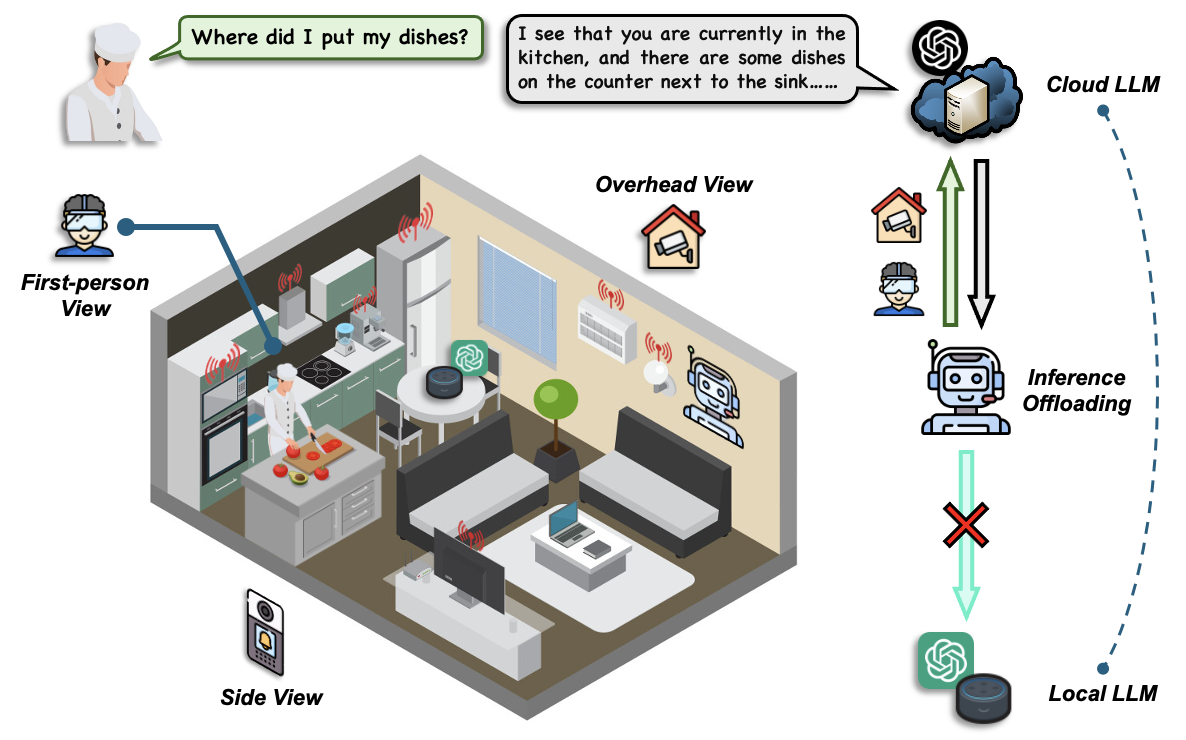
Figure 1: Application Scenario for the LCIO System: Kitchen Activity Assistance with LLM. Upon receiving the user’s text prompt, RL determines the most suitable LLM (i.e., local LLM vs. cloud LLM) and the most relevant data modalities based on the task and previous dialogues. For the specific query, “Where did I put my dishes?” RL identifies that this question is most closely related to the first-person view and overhead view modalities. Consequently, the corresponding prompt and the selected modalities are uploaded to the cloud LLM, which processes the multi-modal inputs to respond to the query. The local LLM, with its limited capability (e.g., processing only text data), may not be able to solve this task.

Motivation. The development of LLMs is thriving, yet deploying LLMs on local devices presents practical challenges, including computational, memory, and energy resources [7, 8, 9, 10, 11]. These hinder the installation of large-scale LLMs locally or real-time, seamless communication with cloud LLMs. These issues hinder the deployment of large-scale LLMs on users’ local devices [12, 13]. Industry giants have developed strategies that either (i) involve lightweight versions of LLMs, such as Google’s Gemma and Meta’s Llama, which offer solutions with varying numbers of parameters (typically 3B, 8B, 13B, etc.) for fast and cost-efficient response, or (ii) place LLMs in the cloud, where users interact with them via the internet, as seen with the ChatGPT application on mobile phones. The former often suffers from inferior inference performance, while the latter requires substantial network bandwidth and incurs high costs from service providers. Therefore, our motivation is to build a system that combines the advantages of both to enhance response quality while ensuring lower latency and usage costs.

Challenges. However, different from traditional machine learning models, achieving this objective with LLMs poses new challenges. LLMs operate in complex environments characterized by (i) multi-modal data sources (i.e., the LLM may need to process different types of data such as text or image to make reliable decisions), (ii) multi-task (i.e., users may want to solve different types of tasks such as message editing or recommendation), and (iii) multi-dialogue (i.e., users engage in multiple interactions with the LLM). Although these elements enrich the capabilities of LLMs, they introduce significant challenges in the inference stage. First, it is challenging to decide the optimal location for inference, i.e., whether to process by the local LLM or to offload tasks to the cloud LLM. This decision critically impacts not only the response quality but also the latency and usage costs. For example, local LLM inference may limit response quality due to the lightweight model deployed on local devices, whereas cloud LLM inference, although potentially more powerful, can introduce significant communication/computation delay [14]. Second, selecting which multi-modal data sources to use for each task/dialogue is non-trivial. Although various types of input data can improve the response quality of LLMs, not all tasks require comprehensive multi-modal data. For example, a message editing task may not require images as inputs, whereas some human activity tasks require various types of image modalities [15, 16, 17]. Deciding which modalities are necessary and how to efficiently process them without incurring excessive delay or cost is a critical aspect of deploying LLMs. Third, due to the expensive nature of LLM inference, online training strategies (i.e., real-time interaction with LLM inference) are often impractical. Consequently, it becomes necessary to generate a dataset for offline training. However, the inherent uncertainty of LLM inference presents additional challenges, as even identical inputs can produce different outputs. This uncertainty significantly exacerbates the difficulty of evaluating LLM outputs, particularly in multi-task or generative tasks where no standard answers or evaluation metrics exist.

Motivated by these, we aim to answer the following question:

In the local-cloud LLM system, (i) how to select the appropriate LLM for inference (i.e., local vs. cloud), (ii) how to choose the most informative and associated multi-modal data sources for each task and dialogue, while taking into account response quality, latency, and usage cost, and (iii) how to address the inherent uncertainty in LLM inference during offline training?

Contribution. We propose a local-cloud inference offloading (LCIO) strategy within a local-cloud LLMs system aimed at enhancing response quality, and reducing latency and usage costs. Fig. 1 illustrates the workflow of LCIO. We address the above research question by developing reinforcement learning (RL) that learns optimal actions in the current state through offline learning of the environment in which users interact with LLMs. The state is determined by the historical information of LLMs and modalities, and the current task (which reflects the task’s difficulty and relevance to the environment). The action involves selecting the LLM and the modalities to answer the aforementioned key research question. Our main contributions can be summarized as follows :

• We design a local-cloud LLM inference offloading system, termed LCIO, to optimize LLMs’ response quality, latency, and usage costs. We implement the LCIO system within a multi-modal, multi-task, multi-dialogue scenario. Specifically, we explore the capabilities of LLMs across various tasks, including assistant, query, recommendation, and message editing, and demonstrate its effectiveness in dynamically adapting to diverse conversational demands (Sec. III-A and Sec. III-B).

• We propose resource-constrained RL (RCRL) to maximize long-term reward when utilizing the LCIO system. By selecting the best LLM and modalities for inference, this approach allows for effective trade-offs between response quality, latency, and usage costs. In addition, the reward takes into account the association between user’s text prompts and other modalities to quantify the connections between tasks and multi-modal data sources, incorporating them into the decision-making process (Sec. III-C).

• We introduce a nearest neighbor strategy for estimating the response quality of uncertain state-action pairs. This approach addresses two types of uncertainty: the non-deterministic evaluation (NDE), where identical state-action pairs can yield varying response quality evaluations, and the out-of-distribution (OOD) scenario, where the system must estimate the response quality for previously unseen state-action pairs. For the first scenario, our strategy provides an estimation of the response quality to reduce the uncertainty introduced by the LLM-as-judge. For the second scenario, it quantifies the potential responses that LLMs may generate when exploring any action in RCRL (Sec. III-D).

• We propose and generate a new dataset termed M4A1, which considers multi-modal, multi-task, multi-dialogue, and multi-LLM characteristics, encapsulating these four “multi” elements all in one dataset. It includes (i) three different view images, (ii) four distinct tasks, (iii) two to five sequential dialogues, and (iv) four LLMs for different purposes. Based on this dataset, we explore the impacts of various RL algorithms, trade-off strategies, resource constraints, local devices, and response quality differences between LLMs to demonstrate the efficacy and versatility of the proposed LCIO system (Sec. IV).

Organization. The remainder of this paper is organized as follows. Sec. II reviews the related work. Sec. III presents our proposed LCIO system along with the design of RCRL. In Sec. IV, we introduce our M4A1 dataset and detail the experimental results. Finally, Sec. V concludes the paper and discusses future research directions.

II Related Work

II-A Efficient LLM on Local Devices

The rapid development of LLMs has profoundly influenced how people interact with AI, yet it also poses multiple challenges related to operational costs, energy consumption, and environmental impact. To mitigate inference overhead, researchers have proposed various solutions. For example, OpenAI has optimized every layer of the stack and introduced an end-to-end multi-modal LLM, GPT-4o, which achieves twice the inference speed and halves the inference cost [18]. Chen et al.[19] have explored strategies such as shrinking prompt sizes, linking multiple queries to share prompts, caching and reusing previous responses, fine-tuning cheaper LLMs with outputs from more expensive ones, and selectively mixing various LLM APIs. Beyond these architectural optimizations, various LLM architectures suitable for local devices [12, 20] and quantization techniques [21] have been proposed to enable deployment in resource-constrained devices.

Other edge-based LLM technologies, such as Apple Intelligence [22], have demonstrated remarkable capabilities on mobile devices, including the integration of ChatGPT into Siri. However, this solution still relies solely on user control to choose which LLM to use, rather than autonomously determining the most appropriate LLM or modality. This limitation is particularly evident when dealing with multiple multi-modal data sources. For example, consider an iPhone equipped with a front camera, a rear camera, and the ability to capture screenshots. The user must manually decide which data source aligns best with the current task (e.g., switching cameras) before uploading the selected content to ChatGPT, thereby introducing inconvenience and operational overhead. Moreover, existing frameworks (i.e., LLM selection strategies) fail to account for the intricate relationships between various modalities and tasks, nor do they consider the context or dialogue history across multiple turns.

II-B LLM Deployment over Network

LLMs over network, such as the ChatGPT application on mobile phones using cellular networks or WiFi, bring the convenience of queries anytime and anywhere to people’s lives, even facilitating multi-modal queries by accessing the phone’s camera [23, 24]. However, this also imposes requirements on the phone’s network connectivity and involves costs for LLM services. Such LLMs over the network present practical challenges for applications that require low latency [25]. For example, [26] discuss using GPT-4 for voice-assisted autonomous driving. The LLM response time is around 1.5 seconds, and there is also the risk of losing connection. Therefore, using LLM over the network can only serve as an assistive tool and is far from sufficient for autonomous driving. Some researchers have proposed solutions to reduce the latency of LLMs over networks. [27] proposed using LLM to generate latency-sensitive code paths during an initial offline phase prior to task execution, rather than during the system’s online operation, to reduce communication latency with cloud LLMs. [28] introduced TREACLE, an RL algorithm that selects different LLMs and prompts based on the inference costs and latency associated with each LLM. However, most existing frameworks either focus solely on one type of resource or only on the accuracy of LLM responding to simple inquiries, without considering the trade-offs and optimization of multiple key resource indicators in multi-modal, multi-task, multi-dialogue scenarios.

II-C Model and Modality Selection

Model and modality selection has been optimized on the basis of a range of criteria such as performance, cost, and latency. This is achieved through decision-making strategies that incorporate objective optimization, simulated annealing, genetic algorithms, among others [29]. Entropy has been used to establish a threshold to decide whether to offload inference tasks to a server [30]. Furthermore, a multi-objective optimization approach has been proposed, which accounts for the Shapley value of different modalities, communication overhead, and the recency of modality selection [31].

Although the aforementioned methods focus primarily on meeting specific performance standards or finding global optimal solutions, they are not designed to consider maximization of cumulative rewards throughout the decision-making process, which is crucial in time-series tasks. [32] developed RL for modality selection in a series of medical diagnostics. This method determines whether to collect additional modality data, which modality to collect, and when to conclude the examination and make a diagnosis, thereby maximizing the trade-off between accuracy and cost. However, this approach does not account for multi-disease diagnostic scenarios, nor does it consider the association between diagnostic content (i.e., disease) and modalities. [33] employed RL to realize resource allocation in LLM inference offloading, yet the approach does not consider multi-modal data or the time-series aspects of multi-dialogues. This omission fails to align with the practical scenarios of using LLMs to solve complex tasks, which typically involve interactions over extended periods and require the processing of diverse types of data. Differently from prior works, we implement these concepts in a multi-dialogue LLM scenario, not only maximizing cumulative rewards, but also considering the relevance between tasks and modalities in a multi-task setting to select the optimal models and modalities.

III Proposed LCIO System

III-A Multi-Task/Dialogue Scenario with Multi-Modal Data

In our problem setting, a user aims to solve multiple types of task through a series of dialogues with the LLM. Each dialogue $t$ involves (i) a text prompt $P_{t}$, such as “Please recommend two dishes that I can cook based on what I have,” and (ii) a set of other modalities $\mathcal{M}$, such as different views of images, 3D points, or other formats of data describing the current situation. During the conversation with the LLM, a user may ask additional questions using prompts potentially related to the previous dialogues: “Where did I put my dishes?” or “Please turn on all the lights in the kitchen” (see Fig. 2). Here, each text prompt belongs to one of the $N$ different task categories, such as assistant, recommendation, query, and message editing. Moreover, distinct tasks have varying levels of difficulty and require different types of multi-modal information to solve. For example, the prompt “Where did I put my dishes?” requires additional modalities (e.g., images) for the LLM to solve the task, while the prompt “Please turn on all the lights in the kitchen” may not require other sources of data, indicating that the task is simpler. These characteristics within a multi-task, multi-dialogue scenario with multi-modal data sources distinguish our setup from many existing works that consider simpler settings (e.g., a single dialogue with text only), motivating the need for a new solution.

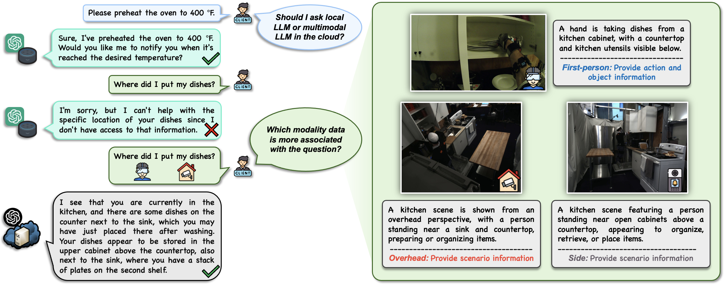
Figure 2: Challenges Emerging in the Local-Cloud LLM Inference. When the user poses questions of varying complexity and scenario information needs, it becomes challenging to determine which LLM and modality(s) should be used for inference. First-person view captures the specific action of the user and the objects but does not reveal the exact location of the cabinet. Overhead view provides information about the entire scenario but lacks details about what the person is specifically doing. Side view, similar to the overhead view, offers scenario information that overlaps in terms of the specific user action.

III-B Local-Cloud LLM Inference

Due to the inherent limitations of local devices in terms of computational resources, memory, and energy consumption, deploying large-scale LLM directly on these devices is often impractical. On the other hand, relying exclusively on cloud-based LLMs can introduce latency and potential usage costs, especially when handling multi-modal data. We propose the local-cloud LLM inference offloading (LCIO) system, as shown in Fig. 1, which strategically distributes tasks between local and cloud platforms to exploit their respective strengths. It consists of two different LLMs: the local LLM and the cloud LLM. The local LLM is a lightweight LLM (e.g., Phi-3-mini [34]) deployed on local devices to handle simple tasks efficiently. This model is optimized for high-speed text prompt processing, suitable for tasks such as message editing, setting timers, or adjusting air conditioning settings, where a sophisticated understanding of multi-modal data is not critical. On the other hand, the cloud LLM is a large-scale multi-modal LLM (e.g., GPT-4o [18]) situated in the cloud capable of managing complex task and multi-modal data that exceed the processing capabilities of local devices. This LLM can integrate multi-modal data input, thus providing richer, more accurate responses where required. The advantage of the LCIO approach is its flexibility and efficiency. In the LCIO system, the user can flexibly choose to either offload inference to the cloud or process it locally, depending on the task’s difficulty and current resource requirements. By offloading computationally intensive tasks to the cloud, we preserve local resources while still benefiting from the cloud’s powerful computational abilities. This configuration allows each part of the system to operate within its capacity, optimizing overall performance and user experience (e.g., latency and costs).

Formally, we describe the interaction with either the local or cloud LLM at each dialogue $t$ as follows:

$$R_{t}=\begin{cases}\text{LLM}_{\text{Local}}\left(P_{t}\right),\ \ \ \text{for local},\\ \text{LLM}_{\text{Cloud}}\left(P_{t}\right),\ \ \ \text{for cloud text-only},\\ \text{LLM}_{\text{Cloud}}\Big{(}P_{t},\bigcup\limits_{m\in\mathcal{M}_{t}}\{D^{(m)}\}\Big{)},\\ \ \ \ \ \ \ \ \ \ \text{for cloud with modalities in $\mathcal{M}_{t}$},\end{cases}$$ (1)

where $R_{t}$, $P_{t}$, and $\mathcal{M}_{t}\subseteq\mathcal{M}$ represent the LLM response, text prompt, and the set of selected modalities uploaded to the cloud, respectively, at dialogue $t$. $D^{(m)}$ denotes the data source of modality $m\in\mathcal{M}$, while $\text{LLM}_{\text{Local}}$ and $\text{LLM}_{\text{Cloud}}$ indicate the local LLM and the cloud LLM, respectively. Thanks to the transformer architecture of LLM, it is capable of maintaining a contextual memory over extended dialogues, thereby allowing the LLM to generate responses for the current prompt based on the accumulated context of all previous prompts and responses. Hence, Eq. (1) can be rewritten to reflect the cumulative nature of the prompts. For example, in the case of the cloud LLM with multi-modal inputs,

$$R_{t}=\text{LLM}_{\text{Cloud}}\left(P_{t},\bigcup_{i=0}^{t}\bigcup_{m\in\mathcal{M}_{i}}\{D^{(m)}\},\bigcup_{i=0}^{t-1}\{P_{i},R_{i}\}\right),$$ (2)

where $t=1,2,\dots,T$. In Eq. (2), in addition to the inputs in Eq. (1), we consider the previously selected modalities as well as prior prompts and responses from the series of earlier dialogues $i=0,1,\dots,t-1$.

Objective of LCIO. The primary objective in deploying the LCIO system is to strategically decide (i) whether to use the local LLM or cloud LLM and (ii) which multi-modal data sources to utilize, for each task or dialogue. This decision-making process aims to enhance response quality while efficiently managing latency and costs throughout extended interactions. The goal is to ensure a seamless user experience in complex multi-dialogue environments, particularly under the constraints of available resources (e.g., latency and costs).

Challenges in LCIO. Fig. 2 summarizes the key challenges of our problem. Selecting the appropriate LLM and modalities for different tasks remains a complex decision, particularly in each dialogue where the choice between utilizing cloud LLM or local LLM is influenced by the distinct difficulties of prompts and the availability of multi-modal data sources. More importantly, while humans may be capable of making short-term decisions for current tasks without history (for example, intuitively deciding to use the local LLM for simple message editing), the challenge intensifies when considering the entire spectrum of interactions over prolonged multi-dialogues. Here, we need to consider response quality, latency, and costs cumulatively throughout the multi-dialogue process. This includes decisions on offloading inference to the cloud, where users need to not only determine which and how many multi-modal data sources to transmit but also balance the quality of the response with other metrics, such as latency and cost. Furthermore, early uploading of modality data to the cloud LLM can facilitate a more quick and nuanced understanding of the environment, which subtly enhances the management of long-term, multi-dialogue interactions.

III-C RCRL for LLM and Modality Selection

We propose a resource-constrained RL (RCRL) approach to make informed decisions regarding the selection between local and cloud LLM services, as well as the determination of which data modalities to be uploaded, as shown in Fig. 3 and Alg. 1. In the following, we describe the details of our RL components.

Environment: The environment is defined by dialogues between the user and the LLM services.

State: The state captures both the history of previous LLM selections and the history of uploaded modalities, along with the current task category $n$. Formally, each state in the state space $\mathcal{S}$ can be visualized as a repeated sequence of the tuple $(\text{LLM},\mathcal{M},n)$, spanning $\tau$ time steps. Thus, we can represent the state space $\mathcal{S}$ as follows:

$$\mathcal{S}=(\text{LLM},\mathcal{M},n)^{\tau},$$ (3)

where LLM indicates the choice between local LLM and cloud LLM. The superscript $\tau$ indicates that there are $\tau$ state components over $\tau$ consecutive dialogues, showing the history of model and modality selections.

Action: The action space consists of the choice between utilizing local or cloud LLM services, as well as the selection of one or multiple data modalities for processing. Therefore, the action space $\mathcal{A}$ can be described as follows:

$$\mathcal{A}=(\text{LLM},\mathcal{M}).$$ (4)

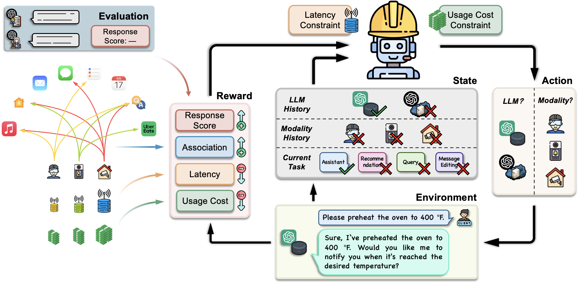
Figure 3: Illustration of RCRL within the LCIO System. The reward computation step is only necessary during the training process. Once the RL policy is deployed, it can determine the appropriate action solely based on the state without processing any external information from the environment (e.g., prompts or responses from the LLM), enhancing the real-time responsibility of the RL action delivery.

Reward: In designing the reward function, we consider several key metrics to optimize the decision-making process regarding the choice of LLM service and modalities. Mathematically, the reward function $\mathcal{R}:\mathcal{S}\times\mathcal{A}\rightarrow\mathbb{R}$ that we propose is expressed as follows:

$$r_{t}=\alpha S_{R_{t}}^{\prime}+\beta_{\Lambda}\sum_{m\in\mathcal{M}_{t}}\Lambda\left(P_{t},D^{(m)}\right)-\beta_{\psi}\psi_{a_{t}}-\beta_{\phi}\phi_{a_{t}},$$ (5)

where:

• Estimated Response Score $S_{R_{t}}^{\prime}$ assesses how effectively the LLM response $R_{t}$ (from either local or cloud) meets the requirements of the text prompt. The response score is used solely for RL training purposes and is not required during the inference phase. A more detailed description of this metric is provided in Sec. III-D.

• Association $\Lambda\left(P_{t},D^{(m)}\right)$ quantifies the relevance of the multi-modal data $D^{(m)}$ to the prompt $P_{t}$. We aggregate the association scores for the set of uploaded modalities $\mathcal{M}_{t}$, which depend on the current action $a_{t}$. Further details are provided in Sec. III-E.

• Latency $\psi_{a_{t}}$ represents the latency of the LLM inference under different actions $a_{t}$. This includes the computation time of the local LLM or the interaction time with the cloud LLM for uploading the selected data modalities. Refer to Sec. III-F for the formal definition.

• Usage Cost $\phi_{a_{t}}$ reflects the cost of LLM under different actions $a_{t}$, including the energy consumption of the local LLM or the service fee of the cloud LLM for various uploaded modalities, as described in Sec. III-G.

The estimated response score $S_{R_{t}}^{\prime}$ and the association $\Lambda\left(P,D^{(m)}\right)$ are considered positive indicators (higher is better, $\uparrow$). In contrast, latency $\psi_{a_{t}}$ and usage cost $\phi_{a_{t}}$ are treated as negative indicators (lower is better, $\downarrow$). Variables $\alpha$, $\beta_{\Lambda}$, $\beta_{\psi}$, and $\beta_{\phi}$ are weighting factors that adjust the influence of each component on the total reward, allowing the system to prioritize different aspects according to specific operational goals and constraints.

Markov Decision Process (MDP) and Optimization: Based on our state and action definitions, we can model this problem as an MDP, where the learning objective is to maximize the cumulative reward, similar to other RL works. In each dialogue $t$, RL algorithms observe the state $s_{t}$, select an action $a_{t}$, obtain a transition probability $P(s_{t+1}|s_{t},a_{t})$, receive a reward $r_{t}$, and transition to the next state $s_{t+1}\sim P(\cdot|s_{t},a_{t})$. Given the current state $s\in\mathcal{S}$, the action $a\in\mathcal{A}$ is selected according to a specific policy $\pi$ as $a\sim\pi(\cdot|s)$, where $\pi(a|s)$ represents the probability of selecting the action $a$ in state $s$. The value function $V^{\pi}(s)$ and the action-value function $Q^{\pi}(s,a)$, respectively, predict the expected discounted rewards of states and actions, following the policy $\pi$:

$$V^{\pi}(s)=\mathbb{E}_{\pi}\left[\sum_{t=0}^{T}\gamma^{t}r_{t}\bigm{|}s_{0}=s\right],$$ (6)

$$Q^{\pi}(s,a)=\mathbb{E}_{\pi}\left[\sum_{t=0}^{T}\gamma^{t}r_{t}\mid s_{0}=s,a_{0}=a\right].$$ (7)

The policy is parameterized by $\theta$ and the optimization of policy $\pi_{\theta}$ aims to maximize the expected discounted rewards:

$$\max_{\theta}J(\theta)\triangleq\mathbb{E}_{s,a\sim\pi_{\theta}}\left[\sum_{t=0}^{T}\gamma^{t}r_{t}\right].$$ (8)

In deep RL optimization, various strategies can be employed to adjust the parameters $\theta$ of the policy $\pi_{\theta}(a|s)$ with the goal of maximizing the performance metric $J(\theta)$. To achieve this, a loss function $f(\theta)$ is defined such that minimizing $f(\theta)$ leads to maximizing $J(\theta)$. Taking Advantage Actor Critic (A2C) [35] as an example, the loss function $f_{\text{A2C}}(\theta)$ includes both the policy loss and the value loss, along with an entropy term to encourage exploration:

$$f_{\text{A2C}}(\theta) =\mathbb{E}_{s,a\sim\pi_{\theta}}[-\log\pi_{\theta}(a|s)A(s,a)$$ (9)

$$+\frac{1}{2}(V^{\pi_{\theta}}(s)-r)^{2}-\zeta H(\pi_{\theta}(\cdot|s))],$$

where $A(s,a)=r+\gamma V^{\pi_{\theta}}(s^{\prime})-V^{\pi_{\theta}}(s)$ is an estimate of the advantage function, providing a measure of the relative value of taking action $a$ in state $s$. The coefficient $\zeta$ controls the weight of the entropy bonus $H(\pi_{\theta}(\cdot|s))$. In Sec. IV-B, we also consider Proximal Policy Optimization (PPO) [36] and Deep Q Network (DQN) [37] versions of Eq. (9).

Algorithm 1 Proposed LCIO System

Input: M4A1 Dataset ($\mathcal{D}$), initial policy parameters ($\pi_{\theta}$), reward weights ($\alpha$, $\beta_{\Lambda}$, $\beta_{\psi}$, $\beta_{\phi}$), time span ($\tau$), resource constraint penalty coefficient ($\lambda$), number of neighbors for response score estimation ($k$), learning rate ($\eta$)

Output: Refined policy $\pi_{\theta}$ for LLM and modality selection

1:for each time step do

2:  Sample a mini-batch of transitions $\{(s,a,s^{\prime})\}$ and corresponding metrics $\{(\Lambda,S_{R},\psi_{a},\phi_{a})\}$ from $\mathcal{D}$. $\triangleright$ Alg. 2

3:  Predict actions $a^{\prime}$ for new states $s^{\prime}$ via the policy $\pi_{\theta}(s^{\prime})$.

4:  Estimate uncertain response scores $S_{R}^{\prime}$ for pending state-action pairs $(s^{\prime},a^{\prime})$ via nearest neighbor. $\triangleright$ Eq. (12)

5:  Compute rewards $r$ based on the estimated response scores $S_{R}^{\prime}$, associations $\Lambda$, latencies $\psi_{a}$, and usage costs $\phi_{a}$. $\triangleright$ Eq. (5)

6:  Calculate the RL loss $f(\theta)$, latency penalty $g_{1}(\theta)$, and usage cost penalty $g_{2}(\theta)$. $\triangleright$ Eq. (11)

7:  Update the policy parameters: $\theta\leftarrow\theta-\eta\nabla_{\theta}F(\theta)$.

8:end for

Resource-Constrained RL (RCRL): A key challenge in non-resource-constrained RL is the unrestricted maximization of rewards, leading to excessive resource use. Even when penalties like latency and usage costs are included in the reward function, they may not enforce strict resource limits, risking over-utilization. To ensure adherence to resource constraints, we incorporate RCRL to enhance decision-making capabilities in environments with limited resources. RCRL involves not only maximizing cumulative rewards, but also satisfying certain constraints on resource consumption such as latency or usage cost. Formally, we embed resource constraints into MDP by introducing a resource consumption function $C(a)$, which quantifies the resources consumed when action $a$ is taken in state $s$. The objective of RCRL is to minimize the loss function $f(\theta)$ (e.g., Eq. (9) for the A2C loss) while ensuring compliance with resource constraints, by solving

$$\min_{\theta}f(\theta)\quad\mathrm{s.t.}\quad\sum_{i=t}^{t+\tau}C_{j}(a_{i})\leq\xi_{j},\;\text{for all}\;j\in\mathcal{J},$$ (10)

where $C_{j}(a)$ denotes the consumption of the $j$-th constrained resource with $\xi_{j}$ as the corresponding threshold, and $\mathcal{J}$ is the set that contains all constraints. $\tau$ is a time span, defined in Eq. (3). We transform resource constraints into a policy optimization problem using a penalty term to enforce constraints. Specifically, we define $g_{j}(\theta)\triangleq\sum_{i=t}^{t+\tau}C_{j}(s_{i},a_{i})-\xi_{j}$ to penalize constraint violations and aim to minimize the following overall loss $F(\theta)$:

$$F(\theta)=f(\theta)+\lambda\sum_{j}\max\left\{g_{j}(\theta),0\right\},$$ (11)

where $\lambda$ denotes the penalty coefficient associated with the constraints. In our experiments, we consider two constraint penalty terms $g_{1}(\theta)$ and $g_{2}(\theta)$ on latency and usage cost, respectively.

III-D Uncertain Response Score Estimation

Due to the enormous number of parameters in LLM, most LLM-related training strategies, such as RLHF and similar approaches, adopt offline training to mitigate substantial inference costs [38, 39]. Similarly, the RCRL framework in our LCIO system also requires learning and exploration of LLM performance in multi-modal, multi-task, and multi-dialogue settings, making a dedicated dataset essential for training RCRL. Given the nature of multi-task settings, particularly in generative tasks, there are often no explicit evaluation metrics, such as accuracy, task success rate, or error rate. This creates a significant challenge in assessing the quality of LLM responses. Moreover, human annotations are not only costly but also inconsistent, individuals evaluating the same LLM response may provide differing assessments, and these variations become even more pronounced across different evaluators, further complicating the evaluation of response quality. In addition, the exploratory nature of RL introduces scenarios, where specific state-action pairs may not exist in the dataset, posing further challenges for quality assessment.

To address these issues, we propose using LLM-as-judge to evaluate response quality. Following this, we employ a nearest neighbor strategy to estimate uncertain response scores, providing a method for handling the inherent uncertainties in outputs of local/cloud LLMs and the judge LLM.

Response Quality Evaluation. The response score $S_{R_{t}}$ measures the response quality generated by the selected LLM in each dialogue. In multi-task scenarios, evaluating the response quality goes beyond merely verifying control actions within an assistant system; it critically involves assessing the actual utility of responses in aiding human users, particularly in query tasks. We utilize the quantitative evaluation scheme outlined by [40, 41, 42], as illustrated in Fig. 4. This involves using two additional text-only LLMs specifically to assess the quality of candidate LLM services. The reference LLM processes a prompt and a reference response to produce a polished reference response, serving as a benchmark for evaluation. The judge LLM then evaluates both the candidate’s response and the reference response, scoring them based on helpfulness, relevance, accuracy, and detail to derive the response score $S_{R_{t}}$, which is calculated as the ratio of the candidate’s LLM score to the reference score.

Uncertain Response Score Estimation. Integrating RCRL directly into real-time LLM inference is impractical, especially in our scenario where four LLMs operate in tandem: local and cloud-based LLMs generate responses, while reference and judge LLMs evaluate their quality. Consequently, we first archive the LLM inference processes into a dataset for subsequent offline RCRL. However, this approach introduces two main forms of uncertainty: (i) non-deterministic evaluation (NDE), in which identical state-action pairs can yield different response quality scores; and (ii) the potential presence of out-of-distribution (OOD) state-action pairs in the dataset. In contrast to [43], which aims to avoid selecting OOD actions, our goal is to more accurately estimate response quality under OOD actions rather than constrain them. This is because the states and actions in our M4A1 dataset are randomly generated (e.g., the current task, selected LLM, and selected modality), making it inevitable that some state-action pairs will not appear in the dataset. To address these uncertainties, we estimate the response score $S_{R}^{\prime}$ for a pending state-action pair $(s^{\prime},a^{\prime})$ by leveraging its nearest neighbors in the dataset. Specifically, let $\{(s_{i},a_{i})\}_{i=1}^{k}$ be the $k$ state-action pairs nearest to $(s^{\prime},a^{\prime})$ in Euclidean distance, and let $\{S_{R_{(i)}}\}$ denote their known response scores. We then estimate $S_{R}^{\prime}$ as a weighted average:

$$S_{R}^{\prime}=\frac{\sum_{i=1}^{k}\mathrm{w}_{i}\cdot{S_{R}}_{(i)}}{\sum_{i=1}^{k}\mathrm{w}_{i}}\quad\mathrm{s.t.}\quad\min_{(s_{i},a_{i})}\left\|(s^{\prime},a^{\prime})-(s_{i},a_{i})\right\|,$$ (12)

where $\mathrm{w}_{i}=\frac{1}{\|(s^{\prime},a^{\prime})-(s_{i},a_{i})\|}$ represents the weight assigned to each known state-action pair $(s_{i},a_{i})$, inversely proportional to their distance from $(s^{\prime},a^{\prime})$. In this way, we achieve a more robust offline estimation of response quality, effectively handling both NDE and OOD uncertainties within RCRL for LLM inference.

III-E Association of Task and Multi-modal Data Source

LCIO is designed to operate in multi-modal, multi-task scenarios. In such settings, it is important to quantify the relevance between user’s text prompts and multi-modal data sources. This helps the user select the most pertinent data modalities to offload to the cloud LLM along with the text prompt for inference. To facilitate this, we introduce an association metric to gauge the relevance of each data modality to the content of the text prompt. Consequently, we employ feature extractors to transform both tasks and modalities into feature vectors of the same dimensionality, which are then used to compute their similarity. Given this premise, we propose leveraging pre-trained CLIP model [44], a transformer-based model comprising a text encoder and an image encoder, to extract features from prompts and multi-model data sources. The pre-trained CLIP has been extensively trained on a vast array of image-text pair data, effectively linking visual concepts with text. In contrast to traditional image classifiers trained on fixed datasets like ImageNet, CLIP can handle both text and images, and has been widely proven to be applicable to nearly any visual classification task. We employ a normalized cross-modality similarity metric to calculate the association score between the text prompt $P$ and the data modality $m$, which is defined as:

$$\Lambda\left(P,D^{(m)}\right)=\frac{\left\langle\omega_{T}(P),\omega_{I}(D^{(m)})\right\rangle}{\left\|\omega_{T}(P)\right\|\cdot\left\|\omega_{I}(D^{(m)})\right\|},$$ (13)

where $\omega_{T}:P\rightarrow\mathbb{R}^{d}$ and $\omega_{I}:D^{(m)}\rightarrow\mathbb{R}^{d}$ represent the text and image encoder functions, respectively, mapping inputs to a shared $d$-dimensional embedding space. The denominator ensures normalization through $L_{2}$ norms, producing similarity scores bounded in $[-1,1]$.

III-F Latency Model

Local Computational Latency $\psi_{\text{Local}}$. The computational latency of the local LLM, or inference time, is influenced not only by the length of the prompt $|P|$ and the response $|R|$, but also significantly by the number of LLM parameters. Following [45, 46], we assume that the computational latency is proportional to the number of parameters, though other latency models can be easily applied. For our local LLM, comprising $|\text{LLM}_{\text{Local}}|$ parameters and requiring $2|\text{LLM}_{\text{Local}}|$ floating point operations for forward propagation, the computational demand for each token in a basic processing length $|P|_{\text{base}}$ is calculated as $\frac{2|\text{LLM}_{\text{Local}}|}{|P|_{\text{base}}}$ floating-point operations. Additionally, other functions may also describe the relationship between the number of parameters and latency, reflecting the complexity of the model and the efficiency of the hardware. The latency calculation considers the theoretical peak performance of the local device’s GPU, $TF_{\text{peak}}$ TFLOPS, leading to the computational latency being defined as:

$$\psi_{\text{Local}}=\frac{2|\text{LLM}_{\text{Local}}|(|P|+|R|)}{|P|_{\text{base}}\times TF_{\text{peak}}}.$$ (14)

Cloud Interaction Latency $\psi_{\text{Cloud}}$. The interaction time with the cloud LLM encompasses the entire process from sending the prompt to receiving the response. This includes uploading the prompt and modalities, inference by the cloud LLM, and downloading the response. We record the interaction time with the cloud LLM $\psi_{\text{Cloud}}$, for different sets of uploaded modalities $\mathcal{M}$, as described in Section IV-A.

Algorithm 2 M4A1 Dataset Collection

Input: Local LLM, cloud LLM, reference LLM, judge LLM, image dataset (e.g., ActionSense), instruction dataset, time span $(\tau)$

Output: M4A1 dataset

1:while collecting data do

2:  Randomly select a moment in the scenario and retrieve images with various modalities.

3:  for a random number of dialogues from 2 to $\tau$ do

4:    Randomly select a user prompt from the instruction dataset.

5:    Randomly choose either the local LLM or the cloud LLM.

6:    if the chosen LLM is the cloud LLM then

7:    Randomly select which modality (text-only, a single view, or multiple views) to upload to the cloud LLM.

8:    end if

9:    Generate a response using the selected LLM based on the context of prior dialogues, the current prompt, and the selected modality.

10:$\triangleright$ Eqs. (1), (2)

11:    The reference LLM generates a reference response based on the prompt and a human-generated reference response.

12:    The judge LLM assigns a response score given the prompt, the candidate response, and the reference response.

13:    Compute the local latency $\psi_{a}$ or record the real interaction time with the cloud LLM provider. $\triangleright$ Eq. (14)

14:    Compute the usage cost $\phi_{a}$ for either the local or cloud LLM. $\triangleright$ Eqs. (15), (16)

15:  end for

16:  for each prompt $P$ and each multimodal data $D^{(m)}$ in the current sample do

17:    Compute the association $\Lambda(P,D^{(m)})$ by the pre-trained CLIP model. $\triangleright$ Eq. (13)

18:  end for

19:end while

III-G Usage Cost Model

During the inference process, LLMs incur computational costs. For the local LLM, it manifests as energy consumption, while for the cloud LLM, it translates into the service fee paid to the providers. The costs associated with running LLMs are determined by factors such as computational complexity, processing duration, and computing equipment.

Local LLM Usage Cost $\phi_{\text{Local}}$. The energy consumption of the local LLM is influenced by inference time and the power consumption of the computing hardware, which are in turn affected by the local device’s computational capacity, the sizes of the prompt and response, and the size of the LLM, all encapsulated within the inference time $\psi_{\text{Local}}$. For a given local device hardware, the maximum power consumption is $W_{\text{max}}$ watts. Furthermore, by utilizing energy costs $\kappa$ (such as local electricity rates) and after appropriate unit conversion, the local LLM usage cost (in USD) is defined as:

$$\phi_{\text{Local}}=\psi_{\text{Local}}\times W_{\text{max}}\times\kappa.$$ (15)

Cloud LLM Usage Function $\phi_{\text{Cloud}}$. For cloud-based LLMs, in addition to the inference costs of prompts and responses, the inference costs of data modalities must also be considered. These costs are typically available on the service provider’s website. Taking GPT-4o as an example, the prompt cost rate is $\varphi_{P}=\$0.005/1K$ tokens, the response cost rate is $\varphi_{R}=\$0.015/1K$ tokens, and the data modality costs are depending on size and resolution. Therefore, the usage cost of the cloud LLM can be defined as follows:

$$\phi_{\text{Cloud}}=\varphi_{P}\left(|P|\right)+\varphi_{R}\left(|R|\right)+\sum_{m\in\mathcal{M}}\varphi_{m}\left(\big{|}D^{(m)}\big{|}\right).$$ (16)

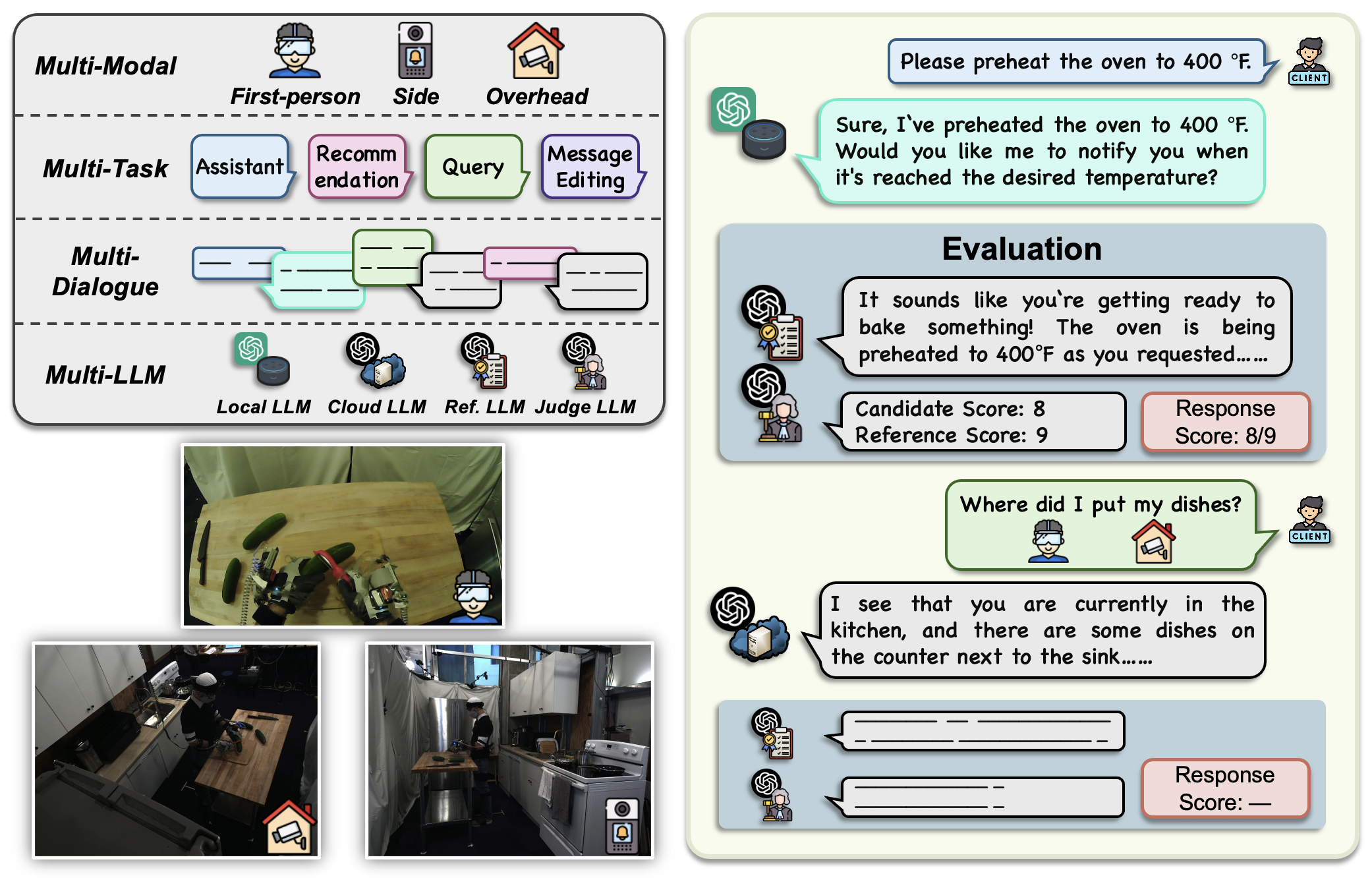
Figure 4: Illustration of M4A1 Dataset. Multi-modal data include first-person view, side view, and overhead view. Client’s prompt dialogues represent four tasks, labeled as Assistant, Recommendation, Query, and Message Editing. LLMs’ dialogues originate from different LLMs, specifically Local LLM and Cloud LLM. According to the evaluation by the judge LLM, Response Score is used to quantify the response quality of the candidate LLMs.

IV Experimental Results

IV-A M4A1 Dataset Construction

IV-A1 Overview of Proposed M4A1

To evaluate performance in practical settings, we develop M4A1, the first multi-modal, multi-task, multi-dialogue, and multi-LLM dataset. The data collection method is detailed in Alg. 2, and an overview of M4A1 is depicted in Fig. 4. M4A1 consists of 6000 samples, each meticulously compiled by randomly and sequentially choosing tasks, prompts, modalities, and candidate LLMs to ensure comprehensive coverage across different configurations. The key characteristics of M4A1 can be summarized as follows:

• Three Multi-Modal Data Sources consist of images from different views in a unified scenario, including first-person, side, and overhead views.

• Four Tasks include Assistant, Recommendation, Query, and Message Editing, represent varying levels of task difficulty, relevance to modalities, and the types of actions that the LLM will undertake.

• Two to Five Dialogues include pairs of text prompts and responses within a continuous context.

• Four LLMs contain a local LLM (Phi-3-mini [34]), a cloud LLM (GPT-4o [18]), a reference LLM (GPT-4o), and a judge LLM (GPT-4o).

• Four Metrics include response score (Sec. III-D), association (Sec. III-E), latency (Sec. III-F), and usage cost (Sec. III-G).

IV-A2 M4A1 Construction Details

To construct the M4A1 dataset, we integrate two predetermined datasets that provide complementary modalities, images and text. First, we use the ActionSense dataset [47] to provide images, offering various camera views of human along with labels for each kitchen activity within the scenario, as illustrated in the bottom left of Fig. 4. ActionSense is a large dataset of human kitchen activities that includes multi-modal wearable sensor data and environmental camera data, capturing 20 different kitchen activities such as peeling cucumbers, slicing potatoes, and cleaning plates with a sponge. These annotated kitchen activity labels function as responses to queries such as “What activity am I doing right now?” Given that current LLMs rarely process time-series sensor data (such as data from gyroscopes and accelerometers), we consider three types of image modalities: first-person images from a wearable sensor, and side and overhead views from environmental cameras. Second, the instruction dataset is used to provide structured text data, enriching the dataset with linguistic elements crucial for LLM inference and evaluation. This dataset provides text for four different tasks with prompts and reference responses. Each task contains five unique prompts, with examples in Fig. 5. For each prompt, a reference response is also provided. Note that the reference responses do not affect the evaluation because the reference LLM will reprocess the content and format of the reference responses.

Each sample in M4A1 is constructed based on a set of three multi-modal data from ActionSense, paired with multiple randomly selected prompt and reference response pairs from the instruction dataset.

I’m feeling a little hot right now, please turn the temperature down a bit. Please play some Christmas music. Please turn on all the lights in the kitchen.

Please recommend some music for me to play right now. Please recommend two dishes that I can cook based on what I have. What is the next recommended step for finishing the meal I am cooking?

What activity am I doing right now? Where did I put my dishes? What are the calorie counts for potatoes and cucumbers?

Please draft a text message asking my friend to bring some ketchup… Please draft a memo to remind me to buy some eggs tomorrow. Please send a message to my home that I’m stuck in traffic and will be home in…

Figure 5: Exemplary Samples in the Instruction Dataset. The dataset consists of prompts that fall into one of the following task categories: Assistant, Recommendation, Query, and Message Editing.

IV-B Experiment Setup

Training Setup. The M4A1 dataset is split into a training set and a test set in an 8:2 ratio. The training set is used to train RLs while the test set is used to evaluate the performance at inference. When implementing our approach, we consider several popular discrete RL algorithms, including PPO [36], DQN [37], and A2C [35]. We consider these methods with and without resource constraints (corresponding to cases with $\lambda>0$ and $\lambda=0$ in Eq. (11)), and denote RC-PPO, RC-DQN, and RC-A2C as the methods with the resource constraints. The policies are parameterized by multilayer perceptrons (MLP), with a total of 30,000 time steps set for training. Default parameters are used as specified in the Stable Baselines3 library [48]. For each experiment, we repeat the process three times and report the standard deviation as the error bar. We implement the LCIO system and the baselines on PyTorch and conducted the experiments on an NVIDIA A100 GPU with 40 GB of memory.

TABLE I: Main Result - LCIO with RC-A2C achieves a balance between local and cloud LLMs while adaptively selecting modalities. It outperforms all baselines with superior response scores, reduced latency, and lower usage costs, without any constraint violations.

Method	Response	Latency	Usage Cost	Overall	Local	Cloud - Num. Selected Modalities 1				Constraint Violation 2 ($\downarrow$)
	Score ($\uparrow$)	(s) ($\downarrow$)	(1e-3 USD) ($\downarrow$)	Reward ($\uparrow$)		0 (text-only)	1	2	3	Latency	Usage Cost
Random	0.86 $\pm$0.02	10.00 $\pm$0.25	12.32 $\pm$0.23	0.71 $\pm$0.01	2097	261	775	771	255	0.95 $\pm$0.13	0.89 $\pm$0.83
Local	0.74 $\pm$0.04	0.04 $\pm$0.00	0.00 $\pm$0.00	0.74 $\pm$0.04	4203	0	0	0	0	0.00 $\pm$0.00	0.00 $\pm$0.00
Cloud	1.04 $\pm$0.01	20.24 $\pm$0.18	25.14 $\pm$0.32	0.75 $\pm$0.01	0	515	1583	1540	544	1.11 $\pm$0.05	2.69 $\pm$0.34
LLM-as-Agent for Inference Offloading (Ignored LLM Agent’s Latency and Usage Cost)
Phi-3-mini	0.81 $\pm$0.04	5.25 $\pm$0.31	7.54 $\pm$0.44	0.74 $\pm$0.04	3089	0	613	207	295	0.00 $\pm$0.00	0.00 $\pm$0.00
Phi-3.5-mini	0.83 $\pm$0.04	5.63 $\pm$0.38	8.39 $\pm$0.57	0.76 $\pm$0.04	3118	0	42	1044	0	0.00 $\pm$0.00	0.00 $\pm$0.00
Llama-3.2-3B	1.05 $\pm$0.02	22.04 $\pm$0.27	35.08 $\pm$0.39	0.74 $\pm$0.02	78	101	58	2955	1011	2.11 $\pm$0.04	4.02 $\pm$0.16
Llama-3.1-8B	0.89 $\pm$0.02	10.84 $\pm$0.18	12.41 $\pm$0.31	0.74 $\pm$0.02	1933	381	1017	545	326	1.54 $\pm$0.22	3.79 $\pm$1.02
Mistral-7B-v0.3	0.83 $\pm$0.03	14.46 $\pm$0.28	1.10 $\pm$0.02	0.64 $\pm$0.03	1519	2684	0	0	0	0.00 $\pm$0.00	0.00 $\pm$0.00
FLAN-T5-large	1.01 $\pm$0.04	24.45 $\pm$0.28	47.91 $\pm$0.55	0.68 $\pm$0.04	0	0	0	0	4203	4.90 $\pm$0.01	11.14 $\pm$0.36
FLAN-T5-xl	0.85 $\pm$0.05	12.95 $\pm$0.15	9.59 $\pm$0.27	0.65 $\pm$0.05	1452	1053	1408	0	289	0.00 $\pm$0.00	0.00 $\pm$0.00
Gemma-2-2b	0.74 $\pm$0.04	0.04 $\pm$0.00	0.00 $\pm$0.00	0.74 $\pm$0.04	4203	0	0	0	0	0.00 $\pm$0.00	0.00 $\pm$0.00
Gemma-2-9b	0.74 $\pm$0.04	0.04 $\pm$0.00	0.00 $\pm$0.00	0.74 $\pm$0.04	4203	0	0	0	0	0.00 $\pm$0.00	0.00 $\pm$0.00
GPT-3.5-turbo	0.99 $\pm$0.02	19.96 $\pm$0.51	33.75 $\pm$0.66	0.73 $\pm$0.01	527	190	504	692	2292	2.97 $\pm$0.15	5.86 $\pm$0.39
GPT-4o-mini	0.74 $\pm$0.04	0.04 $\pm$0.00	0.00 $\pm$0.00	0.74 $\pm$0.04	4203	0	0	0	0	0.00 $\pm$0.00	0.00 $\pm$0.00
GPT-4o	0.85 $\pm$0.05	12.92 $\pm$0.29	0.98 $\pm$0.02	0.67 $\pm$0.05	1807	2396	0	0	0	2.26 $\pm$0.01	0.00 $\pm$0.00
OpenAI o1-mini *	0.77 $\pm$0.03	8.21 $\pm$0.43	0.62 $\pm$0.03	0.66 $\pm$0.03	222	127	0	0	0	1.13 $\pm$0.81	0.00 $\pm$0.00
OpenAI o1 *	0.76 $\pm$0.02	5.18 $\pm$0.16	0.39 $\pm$0.01	0.69 $\pm$0.02	269	80	0	0	0	0.38 $\pm$0.54	0.00 $\pm$0.00
OpenAI o3-mini *	0.86 $\pm$0.04	16.91 $\pm$1.18	1.28 $\pm$0.09	0.63 $\pm$0.03	87	262	0	0	0	2.09 $\pm$0.06	0.00 $\pm$0.00
Comparison with SOTA
AIwRG [33]	1.02 $\pm$0.05	23.73 $\pm$0.98	44.01 $\pm$3.50	0.69 $\pm$0.06	113	244	0	0	3852	4.68 $\pm$0.18	9.26 $\pm$1.83
PerLLM [49]	0.97 $\pm$0.06	21.12 $\pm$0.08	1.60 $\pm$0.01	0.66 $\pm$0.06	281	3922	0	0	0	0.00 $\pm$0.00	0.00 $\pm$0.00
LCIO (PPO)	1.02 $\pm$0.00	17.89 $\pm$0.82	22.48 $\pm$1.48	0.76 $\pm$0.01	142	40	2499	1355	121	0.70 $\pm$0.77	1.66 $\pm$2.35
LCIO (DQN)	1.02 $\pm$0.08	19.57 $\pm$2.18	26.23 $\pm$6.36	0.75 $\pm$0.05	0	5	1820	2367	0	0.81 $\pm$0.57	0.00 $\pm$0.00
LCIO (A2C)	1.05 $\pm$0.03	18.81 $\pm$3.44	26.44 $\pm$13.05	0.79 $\pm$0.07	98	0	2753	210	1168	1.48 $\pm$2.09	2.38 $\pm$3.36
LCIO (RC-PPO)	1.03 $\pm$0.03	18.33 $\pm$1.87	22.43 $\pm$3.57	0.77 $\pm$0.04	90	105	2599	1309	110	0.45 $\pm$0.64	0.00 $\pm$0.00
LCIO (RC-DQN)	1.05 $\pm$0.05	18.87 $\pm$0.81	23.29 $\pm$3.59	0.78 $\pm$0.06	46	174	2249	1636	85	0.53 $\pm$0.33	0.42 $\pm$0.60
LCIO (RC-A2C)	1.09 $\pm$0.08	16.63 $\pm$0.67	17.97 $\pm$1.18	0.85 $\pm$0.07	74	12	3871	225	6	0.00 $\pm$0.00	0.00 $\pm$0.00
Ours LCIO System - Ablation Study (Using RC-A2C as Backbone)
w/o LLM Sel. 3	0.85 $\pm$0.00	9.25 $\pm$1.02	11.67 $\pm$3.14	0.72 $\pm$0.02	2128	6	1228	830	1	0.00 $\pm$0.00	0.00 $\pm$0.00
w/o Modality Sel.	1.04 $\pm$0.02	20.13 $\pm$0.07	24.82 $\pm$0.21	0.75 $\pm$0.02	0	528	1591	1519	528	1.17 $\pm$0.07	2.74 $\pm$0.87
w/o Score Est.	1.01 $\pm$0.01	16.71 $\pm$0.28	17.76 $\pm$0.59	0.76 $\pm$0.01	0	0	4095	89	0	0.00 $\pm$0.00	0.00 $\pm$0.00

¹ Num. Selected Modalities refers to the number of modalities selected in a single dialogue. For example, with two selected modalities, combinations include {first-person, side}, {first-person, overhead}, {side, overhead}.  ² Constraint Violation refers to the instances where the cumulative resource consumption caused by multiple consecutive actions in each sample exceeds the threshold value, as defined by $\max\left\{g_{j}(\theta),0\right\}$ in Eq. (11).  ³ w/o LLM Sel., w/o Modality Sel., and w/o Score Est. refer to without LLM selection, without modality selection, and without uncertain response score estimation, respectively.

^* Due to the considerable inference time and usage cost of OpenAI o1-mini, OpenAI o1, and OpenAI o3-mini, we randomly sample 100 instances for evaluation.

Baselines. We compare the RL algorithms with three naive baselines: random (with random LLM and modality selection), local (using only the local LLM), and cloud (using only the cloud LLM, but with random modality selection). In addition, we replace RL with LLM-as-agent for LLM and modality selection. Specifically, the current state and possible actions are translated into natural language descriptions and provided as contextual input to the LLM agent for decision-making. These LLM agents do not access any information beyond what is provided to RL. The LLM agents include Phi-3-mini [34], Phi-3.5-mini [34], Llama-3.2-3B [6], Llama-3.1-8B [6], Mistral-7B-v0.3 [50], FLAN-T5-large [51], FLAN-T5-xl [51], Gemma-2-2B [3], Gemma-2-9B [3], GPT-3.5-turbo [52], GPT-4o-mini [53], GPT-4o [18], OpenAI o1-mini [54], OpenAI o1 [54], and OpenAI o3-mini [55]. We reiterate that none of the existing works can be directly applied to our setting, which features multi-modal, multi-task, and multi-dialogue characteristics. Therefore, we reimplement AIwRG [33], an active inference method, and PerLLM [49], a bandit-based approach using Upper Confidence Bound (UCB) for exploration-exploitation trade-off, integrating the settings introduced in this paper to adapt them to our research problem.

Default Settings. The default experimental settings are as follows unless otherwise stated; we also study the effects of various system parameters. Specifically, we use RC-A2C for the RL method, with $\alpha=1$, $\beta_{\Lambda}=1/3$, $\beta_{\psi}=1/3$, and $\beta_{\phi}=1/3$ for the reward function weights, a 30 second latency constraint, a 0.05 USD usage cost constraint, and Jetson TX2 as the device type. These settings serve as the baseline from which variations are systematically introduced to assess their effects. Additionally, we set the time span $\tau=5$, the penalty coefficient $\lambda=10$, $k=5$ nearest neighbors for estimating the response score, and $\kappa=4.63\times 10^{-8}$ (Joules per USD) based on the average electricity price in the US .

IV-C Main Experimental Results

Table I presents the main results of this study, with key takeaways described from four perspectives.

Comparison with Naive Baselines. Compared to the local baseline, the proposed methods can significantly improve the response score by sacrificing latency and usage costs, thus enhancing the overall reward. Compared to the cloud baseline, we also boost the response score and conserve resources by selecting the appropriate modalities, which leads to improved rewards. In contrast to Random, our approach strategically explores the relationships between tasks/dialogues and LLMs/modalities, thereby optimizing decision-making processes to better align with the specific requirements and constraints of each task.

Comparison with LLM-as-Agent Baselines Inspired by recent advances in LLM-as-agent [56, 57], we replace the RL component in our LCIO system with an LLM for decision making. Specifically, we design a system prompt to specify the background information, including the objective, output format, and possible actions. The workflow then follows an RL-like procedure: when faced with a particular state, we first convert it into a natural language prompt, after which the LLM agent outputs an action. Our goal is to evaluate the zero-shot LLM agent’s ability to consider modality-task relationships, understand context, and handle numerically sensitive tasks (e.g., avoiding resource constraint violations). To ensure a fair comparison, we do not factor in the latency or cost of the LLM agent here. As shown in Table I, different LLM agents exhibit substantial variability in performance. Some agents ignore all modalities (e.g., Mistral-7B-v0.3, Gemma-2-2b, Gemma-2-9b, GPT-4o-mini, GPT-4o, OpenAI o1-mini, OpenAI o1, and OpenAI o3-mini), while others choose to upload all available modalities for each task (e.g., FLAN-T5-large). Although some agents (e.g., Phi-3-mini, Phi-3.5-mini, and FLAN-T5-xl) appear to select different LLMs and modalities without violating any constraints, their response scores and overall rewards do not confer significant advantages. Thus, these zero-shot LLM agents do not demonstrate clear benefits. One reason is that they are not fine-tuned in the training dataset. Another reason is that, as generative models, LLM agents lack precise numerical calculation capabilities. Consequently, some agents violate constraints, whereas others adopt overly conservative strategies.

Comparison with SOTA Baselines. Existing works do not address multi-task and multi-dialogue settings in a multi-modal scenario. For example, [33] utilizes the HumanEval dataset [58], which focuses on generating Python code based on task descriptions. This dataset uses a fixed evaluation metric, Pass@k, which measures the success rate of passing predefined unit tests. In contrast, our method considers a multi-modal, multi-task, and multi-dialogue setting, introducing challenges related to response score evaluation and uncertainty. To adapt methods such as AIwRG [33], which employs active inference, and PerLLM [49], which uses an upper confidence bound (UCB)-based approach, to our setting, we incorporate certain designs from this paper, including the unique mechanisms for LLM and modality selection. In addition, we replace the Pass@k metric with the average response score for each action in the dataset as the success metric. The results demonstrate that our LCIO system significantly outperforms these SOTA baselines. On the one hand, [33] fails to efficiently select LLMs and modalities, frequently opting to upload all three types of modality data sources for most actions. This results in substantial resource waste and redundancy in uploading unnecessary information to the cloud. On the other hand, [49] rarely considers any modality data, relying solely on the local LLM and text-only cloud LLM. Although this approach avoids violating any resource constraints, it leads to lower response scores, as the LLM lacks access to any information derived from modality data.

Analysis of Our LCIO System. Most RL algorithms prefer to utilize the cloud LLM rather than the local LLM, as the gain in response score from the cloud LLM is much greater than the resource savings achieved by the local LLM. This indicates that GPT-4o, which is used for the cloud LLM, is much powerful than the Phi-3-mini used for the local LLM. Regarding modality selection, few RL algorithms choose a text-only cloud LLM, as it often results in interaction times comparable to or even longer than those with multi-modal inputs. This largely depends on the inference speed of the service provider rather than factors like network bandwidth. A potential reason is that text-only and multi-modal cloud LLMs may operate on different workflows and versions. However, in cases involving multi-modal inputs, we observe that single modality selection often receives preferential treatment by RL algorithms, as it provides valuable information with less latency and lower usage costs compared to selecting two or three modalities. RC-A2C demonstrates the best response scores and overall rewards while ensuring compliance with latency and usage cost constraints. It can be observed that RC-A2C selects as many modalities as possible to maximize the overall reward without violating resource constraints. Additionally, the synchronized updates and low-variance policy gradients of RC-A2C facilitate more stable and smooth policy updates. This method effectively adapts and optimizes resource constraints into the loss function, ensuring that these constraints are not violated.

IV-D Ablation Study

To further validate the effectiveness of our approach, in the last three rows of Table I, we utilize the top-performing RC-A2C as the backbone for ablation studies. Specifically, we remove the LLM selection, modality selection, and uncertain response score estimation components from RC-A2C, respectively. In the case of w/o LLM selection, an LLM is randomly selected, and if a cloud LLM is chosen, RC-A2C determines which modalities to use by sorting the action probabilities. For w/o modality selection, once RC-A2C selects the cloud LLM, the modalities are randomly chosen. For w/o response score estimation, we calculate the average response score of each action in the dataset for training, while still evaluating the test performance using our uncertain response score estimation method.

Compared to using RC-A2C, randomly selecting the LLM results in a degradation of the response score because, in many scenarios, the local LLM lacks the capability to complete the tasks. Randomly selecting the modalities leads to significant increases in latency and usage costs, as unnecessary modalities are uploaded, resulting in redundancy. Lastly, while using the average response score of actions may seem reasonable, it fails to account for the contextual information in the state. Specifically, the state includes historical modality upload information, which is crucial for response score estimation. When the response score estimation excludes this context, the estimation becomes biased, leading to incorrect guidance for the decision-making of the model, ultimately degrading its performance in task allocation and modality selection. The results demonstrate that LLM selection effectively manages tasks of varying difficulty by matching them with LLMs of appropriate capability, while modality selection enhances the alignment between modalities and tasks, thereby minimizing latency and usage costs by avoiding unnecessary uploads. Moreover, uncertain response score estimation leverages the contextual information to provide more accurate response score estimations, enabling the model to make well-informed decisions.

TABLE II: Trade-off between Metrics in Reward Function - Varying weights illustrate preferences for different metrics. More balanced weights results in a high response score and relatively low latency and usage cost.

$\beta_{\Lambda}$	$\beta_{\psi}$	$\beta_{\phi}$	Response	Association	Latency	Usage Cost
			Score ($\uparrow$)	($\uparrow$)	(s) ($\downarrow$)	(1e-3 USD) ($\downarrow$)
0	0	0	0.99 $\pm$0.04	0.41 $\pm$0.05	21.39 $\pm$0.81	32.63 $\pm$3.35
1	0	0	1.01 $\pm$0.05	0.62 $\pm$0.00	24.43 $\pm$0.34	47.87 $\pm$0.66
0	1	0	0.73 $\pm$0.04	0.00 $\pm$0.00	0.04 $\pm$0.00	0.00 $\pm$0.00
0	0	1	0.97 $\pm$0.06	0.00 $\pm$0.00	22.46 $\pm$0.06	1.70 $\pm$0.00
0	0.5	0.5	0.76 $\pm$0.06	0.02 $\pm$0.03	1.59 $\pm$2.20	1.63 $\pm$2.31
0.5	0	0.5	1.05 $\pm$0.07	0.39 $\pm$0.10	21.04 $\pm$1.77	31.91 $\pm$7.11
0.5	0.5	0	0.98 $\pm$0.04	0.55 $\pm$0.05	23.26 $\pm$0.92	42.97 $\pm$3.27
1/3	1/3	1/3	1.09 $\pm$0.08	0.21 $\pm$0.01	16.63 $\pm$0.67	17.97 $\pm$1.18

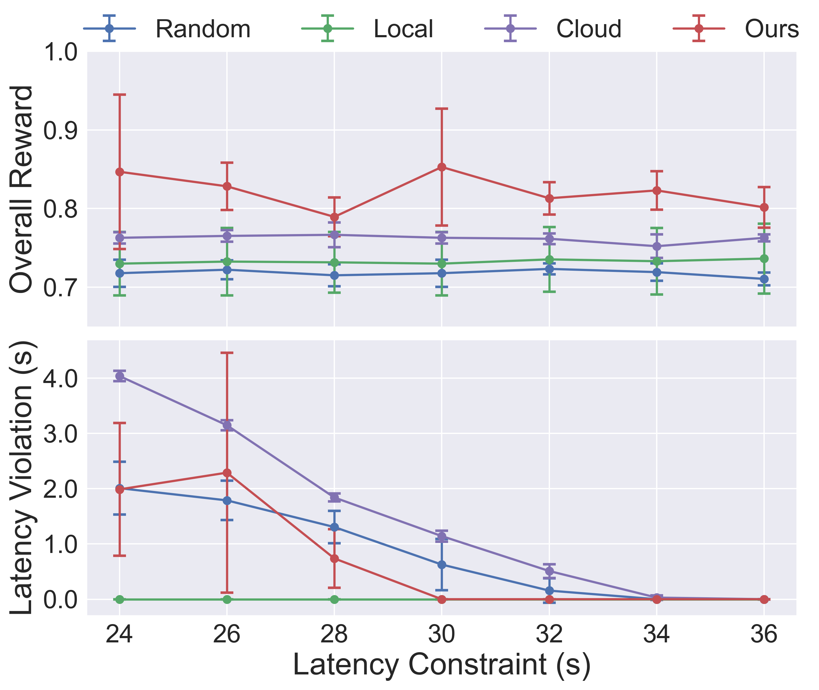
(a)

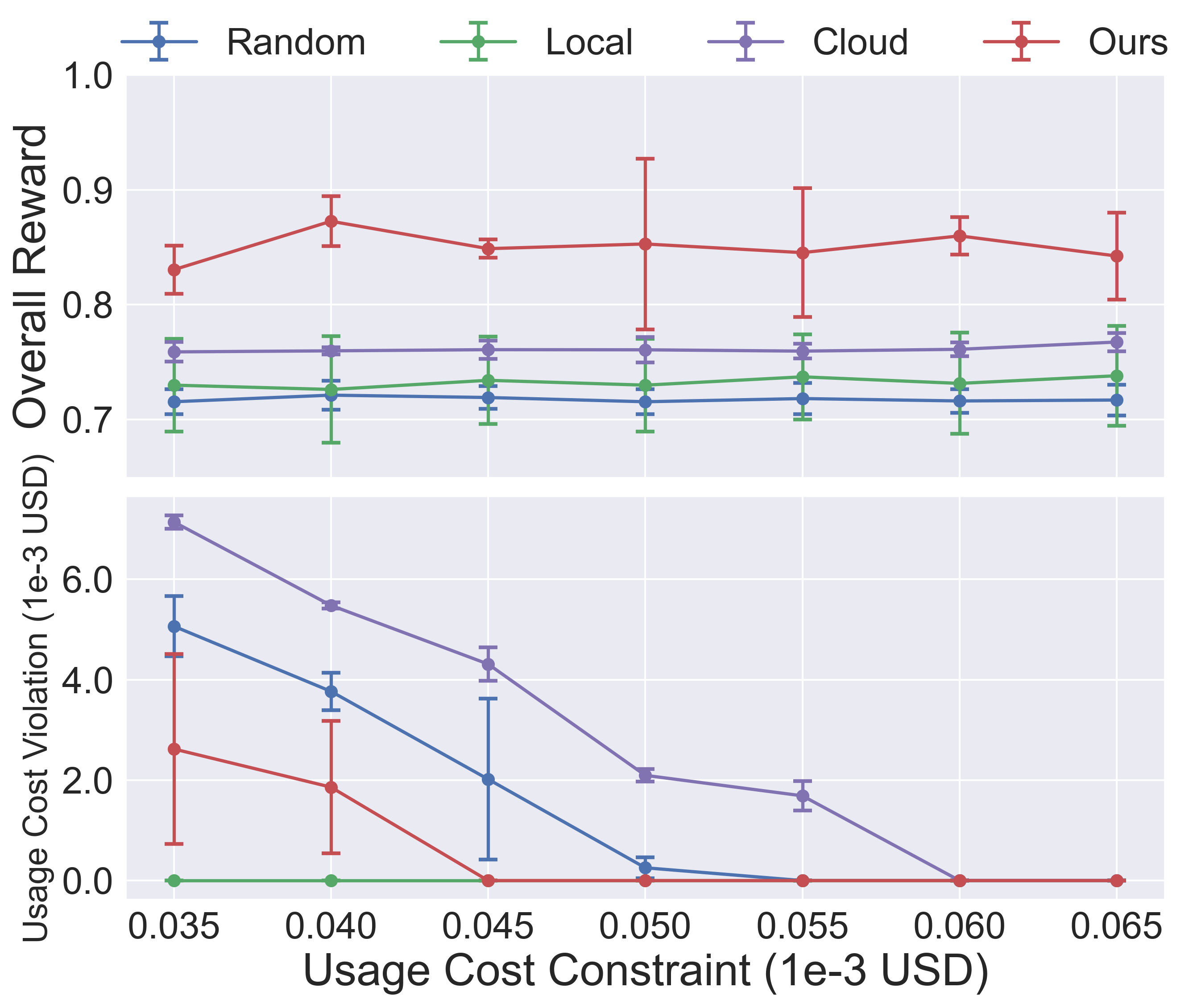
(b)

Figure 6: Effect of Latency and Usage Cost Constraints. Left: Latency Constraint. Right: Usage Cost Constraint. LCIO demonstrates a faster reduction in resource constraint violations compared to baselines.

IV-E Trade-off Between Metrics

In Table II, we investigate the trade-offs among different metrics in the reward function by adjusting the weights for association, latency, and usage cost in Eq. (5), denoted as $\beta_{\Lambda}$, $\beta_{\psi}$, and $\beta_{\phi}$, respectively. We fix the weight of the response score to $\alpha=1$, as in Table I. We observe that neglecting any of these metrics leads to a degradation in the corresponding performance measure. For example, setting $\beta_{\Lambda}=0$ results in a lower response score because the association between the prompt and modalities is not considered. Furthermore, due to the presence of resource constraints, simply setting $\beta_{\psi}=0$ or $\beta_{\phi}=0$ not only causes high latency or high usage costs, respectively, but also does not provide a benefit to the response score. Although the RL model is penalized by the resource constraint in the loss function, it lacks explicit action-level penalties. As a result, the model may only account for cumulative costs, rather than recognizing the cost of individual actions. Concretely, uploading three modality data sources one at a time or uploading all three at once incurs roughly the same total resource cost. Consequently, when we balance the weights by setting $\beta_{\Lambda}=\frac{1}{3},\beta_{\psi}=\frac{1}{3},\beta_{\phi}=\frac{1}{3}$, we can attain a high response score while maintaining relatively lower latency and usage costs.

TABLE III: Local Devices Setting

Local Device	Performance	Power	Latency	Usage Cost
	(TFLOPS)	(Watts)	(s)	(1e-3 USD)
Raspberry Pi-4B	0.0135	8	1.12593	4.17e-4
Raspberry Pi-5	0.0314	12	0.48408	2.69e-4
Jetson Nano	0.472	10	0.03220	1.49e-5
Jetson TX2	1.33	15	0.01143	7.94e-6
Jetson Xavier NX	21	20	0.00072	6.71e-7
Jetson Orin NX	100	25	0.00015	1.76e-7
iPhone 15 (A16)	15.8	15	0.00096	6.69e-04
iPhone 15 Pro (A17 Pro)	35	15	0.00043	3.02e-04

This table details the inference time and usage costs required for local devices to perform a single inference using Phi-3-mini, as calculated by Eqs. (14) and (15). Note that in practical applications, these values are higher due to factors such as other task demands, memory bandwidth, I/O operations, utilization rates, power constraints, etc.

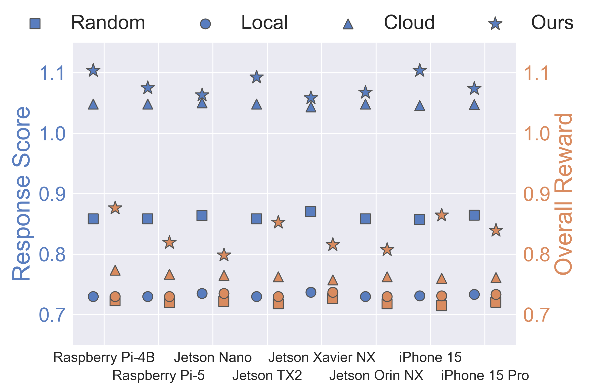
(a)

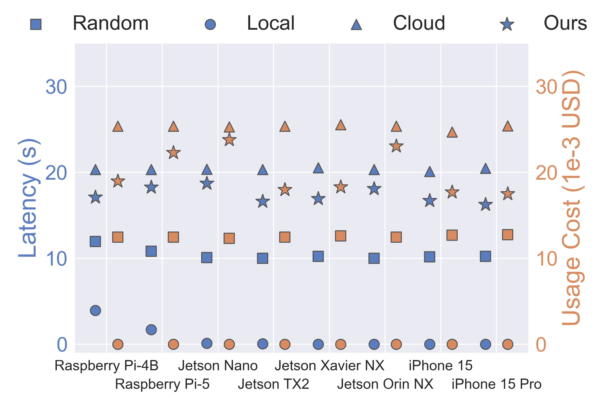
(b)

Figure 7: Effect of Local Device Performance. Left and Right show the same experiment, demonstrating four different metrics. LCIO achieves superior performance on all local device compared to baselines.

IV-F Effect of Resource Constraints

In Fig. 6, we evaluate the performance of different schemes under varying latency and usage cost constraints, reflecting real-world scenarios where applications operate under different budgetary considerations. It is observed that as the settings for latency and usage cost constraints increase, all methods show a reduction in violations of these constraints, with RC-A2C achieving a faster reduction. This improvement is due to the resource constraints that are incorporated in the loss function to balance long-term cumulative rewards. In all different constraint settings, the proposed approach achieves the highest overall rewards, demonstrating its effectiveness in practical system deployments by considering response quality, latency and usage cost altogether. It is noted that even under extremely resource constraints, RC-A2C struggles to balance the trade-off between response score and resource costs effectively. Thus, in practical system deployments, besides employing the resource constraints to optimize long-term cumulative gains, it is also essential to establish safety layers (such as predicting the interaction time and usage cost and interventions directing RL to select local LLM) to mandatory avoid unforeseen high latency and usage costs, especially in time-sensitive applications like autonomous driving.

IV-G Effect of Different Local Device

To further confirm the advantage of our approach, in Fig. 7, we explore the effects of using different types of local devices, including Raspberry Pi, NVIDIA Jetson, and Apple iPhone. Detailed specifications of devices are available in Table III. We infer that the performance of different devices does not significantly affect the operation of the LCIO system, since their response scores and overall rewards do not show statistical significance. The underlying rationality is that for any device, latency and usage cost are normalized through min-max scaling and incorporated as part of the overall reward. The results are consistent with those in Table I, showing that our approach achieves (i) significant latency and cost savings compared to the cloud LLM baseline and (ii) significant improvements in response quality compared to the local LLM baseline, leading to the highest overall reward. Therefore, when the latency and usage costs of a local LLM are substantially lower than those of a cloud LLM, the LCIO system can operate effectively on any device. This precondition forms part of the background for the LCIO system.

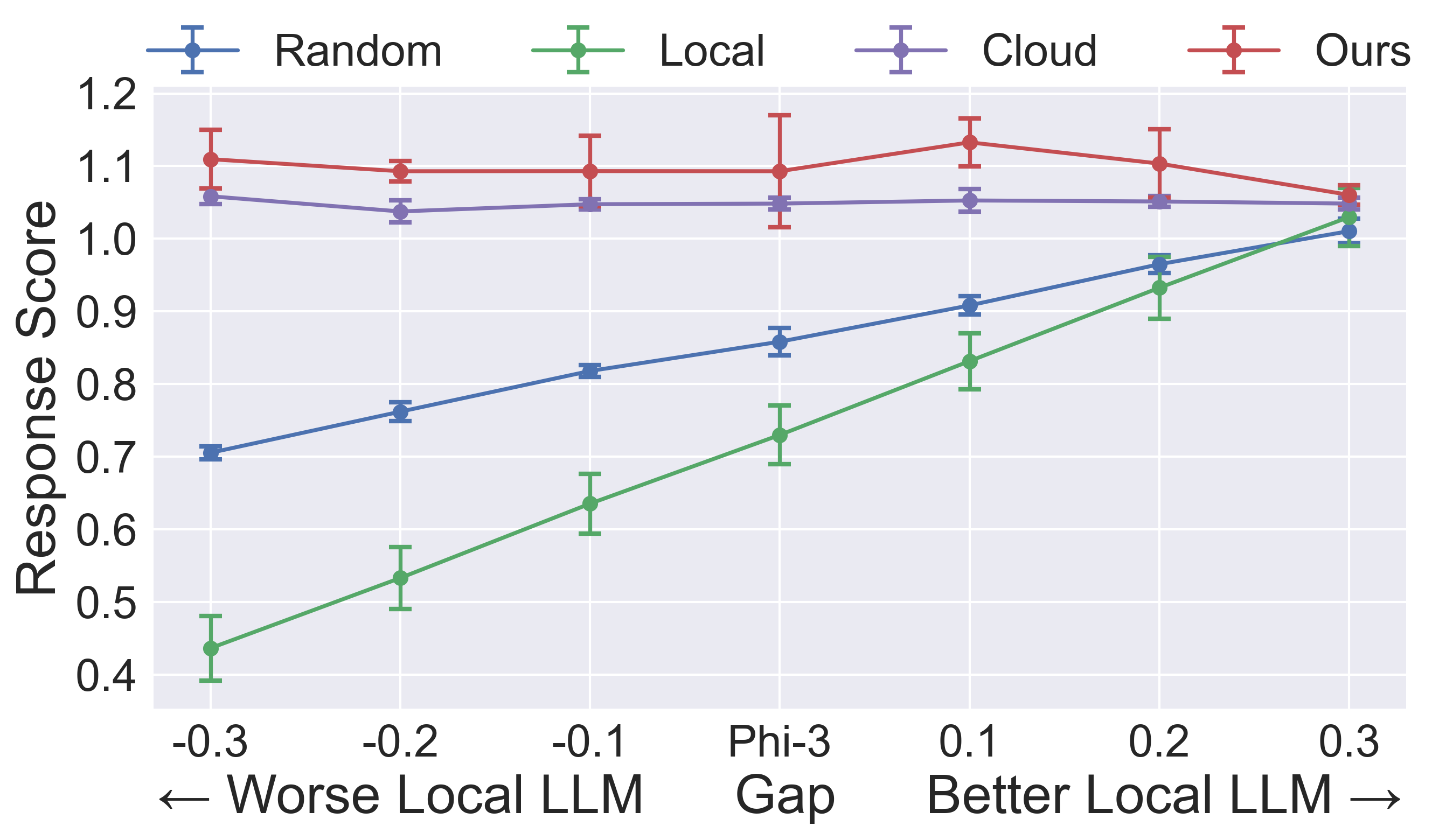
(a)

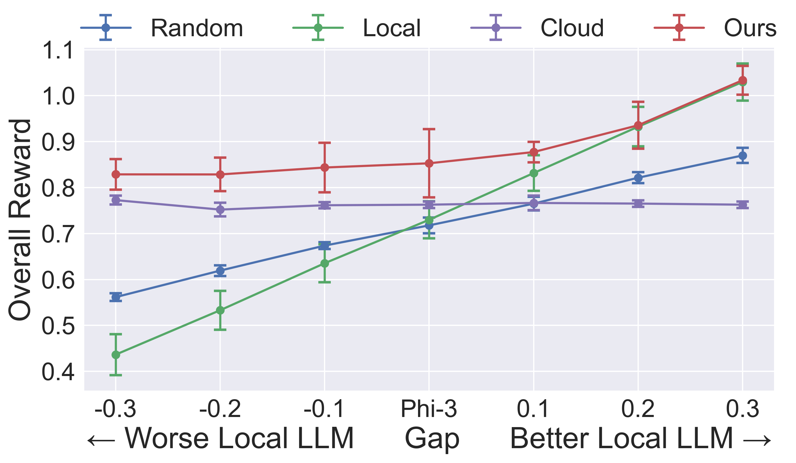
(b)

Figure 8: Effect of Response Quality of Local LLM. Left: Response Score. Right: Overall Reward. LCIO consistently outperforms baselines across various deployments of local and cloud LLMs.

IV-H Effect of Local LLM Response Quality

Finally, we evaluate the performance of the LCIO system by simulating various response qualities of the local LLM. Fig. 8 illustrates the results, where we adjust the response scores of local LLMs in the M4A1 dataset by adding or subtracting specific values (i.e., gap in Fig. 8) to simulate different local LLM capabilities. It is observed that regardless of the response quality of both the local LLM and the cloud LLM, the LCIO system consistently outperforms the three baseline models. This shows that LCIO can operate effectively in any combination of local and cloud LLMs. When the quality of the local LLM response is significantly lower than that of the cloud LLM, LCIO invariably opts for the cloud LLM and proceeds with modality selection. Conversely, as the response quality of the local LLM approaches that of the cloud LLM, LCIO begins to balance between the local and cloud options. An extreme scenario would be using the same LLM both locally and in the cloud, LCIO still capable of delivering superior response quality. This holds under the assumption that the local LLM does not support multi-modal inputs (or, considering a broader perspective, the cloud LLM cannot access user multi-modal data due to privacy concerns), LCIO can leverage the specific needs of certain tasks that require multi-modal data sources for better understanding of the environment. The overall results confirm the applicability of our methodology across a range of local LLM qualities.

V Conclusion

In this paper, we developed LCIO, the first local-cloud LLM inference offloading system designed for multi-modal, multi-task, and multi-dialogue scenarios. We employed RCRL to design the LLM selection and modality selection process to maximize long-term cumulative reward under resource constraints. Furthermore, we constructed a new dataset, M4A1, to evaluate the performance of the LCIO system under various conditions, including different RLs, reward trade-offs, resource constraints, devices, and network scenarios.

Future work will explore collaborative inference offloading among multiple users by developing frameworks that enable resource sharing, cooperative decision-making, and task partitioning to enhance system-wide efficiency and scalability. Additionally, we will investigate further options when a user is faced with multiple cloud service providers, focusing on adaptive strategies that dynamically select the optimal provider based on factors such as latency, usage cost, data privacy, and service reliability in real-time scenarios.

References

- [1] J. Achiam, S. Adler, S. Agarwal, L. Ahmad, I. Akkaya, F. L. Aleman, D. Almeida, J. Altenschmidt, S. Altman, S. Anadkat et al., “Gpt-4 technical report,” arXiv preprint arXiv:2303.08774, 2023.
- [2] G. Team, T. Mesnard, C. Hardin, R. Dadashi, S. Bhupatiraju, S. Pathak, L. Sifre, M. Rivière, M. S. Kale, J. Love et al., “Gemma: Open models based on gemini research and technology,” arXiv preprint arXiv:2403.08295, 2024.
- [3] G. Team, M. Riviere, S. Pathak, P. G. Sessa, C. Hardin, S. Bhupatiraju, L. Hussenot, T. Mesnard, B. Shahriari, A. Ramé et al., “Gemma 2: Improving open language models at a practical size,” arXiv preprint arXiv:2408.00118, 2024.
- [4] G. Team, R. Anil, S. Borgeaud, Y. Wu, J.-B. Alayrac, J. Yu, R. Soricut, J. Schalkwyk, A. M. Dai, A. Hauth et al., “Gemini: a family of highly capable multimodal models,” arXiv preprint arXiv:2312.11805, 2023.
- [5] H. Touvron, L. Martin, K. Stone, P. Albert, A. Almahairi, Y. Babaei, N. Bashlykov, S. Batra, P. Bhargava, S. Bhosale et al., “Llama 2: Open foundation and fine-tuned chat models,” arXiv preprint arXiv:2307.09288, 2023.
- [6] A. Dubey, A. Jauhri, A. Pandey, A. Kadian, A. Al-Dahle, A. Letman, A. Mathur, A. Schelten, A. Yang, A. Fan et al., “The llama 3 herd of models,” arXiv preprint arXiv:2407.21783, 2024.
- [7] P. Patel, E. Choukse, C. Zhang, Í. Goiri, B. Warrier, N. Mahalingam, and R. Bianchini, “Characterizing power management opportunities for llms in the cloud,” in Proceedings of the 29th ACM International Conference on Architectural Support for Programming Languages and Operating Systems, Volume 3, 2024, pp. 207–222.
- [8] Z. Lin, G. Qu, Q. Chen, X. Chen, Z. Chen, and K. Huang, “Pushing large language models to the 6g edge: Vision, challenges, and opportunities,” arXiv preprint arXiv:2309.16739, 2023.
- [9] M. Xu, H. Du, D. Niyato, J. Kang, Z. Xiong, S. Mao, Z. Han, A. Jamalipour, D. I. Kim, X. Shen et al., “Unleashing the power of edge-cloud generative ai in mobile networks: A survey of aigc services,” IEEE Communications Surveys & Tutorials, 2024.
- [10] M. Xu, W. Yin, D. Cai, R. Yi, D. Xu, Q. Wang, B. Wu, Y. Zhao, C. Yang, S. Wang et al., “A survey of resource-efficient llm and multimodal foundation models,” arXiv preprint arXiv:2401.08092, 2024.
- [11] W. Fang, D.-J. Han, L. Yuan, S. Hosseinalipour, and C. G. Brinton, “Federated sketching lora: On-device collaborative fine-tuning of large language models,” arXiv preprint arXiv:2501.19389, 2025.
- [12] X. Chu, L. Qiao, X. Lin, S. Xu, Y. Yang, Y. Hu, F. Wei, X. Zhang, B. Zhang, X. Wei et al., “Mobilevlm: A fast, reproducible and strong vision language assistant for mobile devices,” arXiv preprint arXiv:2312.16886, 2023.
- [13] W. Yin, M. Xu, Y. Li, and X. Liu, “Llm as a system service on mobile devices,” arXiv preprint arXiv:2403.11805, 2024.
- [14] Y. Wang, K. Chen, H. Tan, and K. Guo, “Tabi: An efficient multi-level inference system for large language models,” in Proceedings of the Eighteenth European Conference on Computer Systems, 2023, pp. 233–248.
- [15] Siri Team, “Deep learning for siri’s voice: On-device deep mixture density networks for hybrid unit selection synthesis,” Apple Machine Learning Journal, 2017.
- [16] G. López, L. Quesada, and L. A. Guerrero, “Alexa vs. siri vs. cortana vs. google assistant: a comparison of speech-based natural user interfaces,” in Advances in Human Factors and Systems Interaction. Springer, 2018, pp. 241–250.
- [17] J. Lee, J. Wang, E. Brown, L. Chu, S. S. Rodriguez, and J. E. Froehlich, “Gazepointar: A context-aware multimodal voice assistant for pronoun disambiguation in wearable augmented reality,” in Proceedings of the CHI Conference on Human Factors in Computing Systems, 2024, pp. 1–20.
- [18] OpenAI, “Hello gpt-4o,” https://openai.com/index/hello-gpt-4o/, 2024.
- [19] L. Chen, M. Zaharia, and J. Zou, “Frugalgpt: How to use large language models while reducing cost and improving performance,” arXiv preprint arXiv:2305.05176, 2023.
- [20] Y. Li, S. Bubeck, R. Eldan, A. Del Giorno, S. Gunasekar, and Y. T. Lee, “Textbooks are all you need ii: phi-1.5 technical report,” arXiv preprint arXiv:2309.05463, 2023.
- [21] J. Lin, J. Tang, H. Tang, S. Yang, W.-M. Chen, W.-C. Wang, G. Xiao, X. Dang, C. Gan, and S. Han, “Awq: Activation-aware weight quantization for on-device llm compression and acceleration,” Proceedings of Machine Learning and Systems, vol. 6, pp. 87–100, 2024.
- [22] T. Gunter, Z. Wang, C. Wang, R. Pang, A. Narayanan, A. Zhang, B. Zhang, C. Chen, C.-C. Chiu, D. Qiu et al., “Apple intelligence foundation language models,” arXiv preprint arXiv:2407.21075, 2024.
- [23] H. Wen, Y. Li, G. Liu, S. Zhao, T. Yu, T. J.-J. Li, S. Jiang, Y. Liu, Y. Zhang, and Y. Liu, “Empowering llm to use smartphone for intelligent task automation,” arXiv preprint arXiv:2308.15272, 2023.
- [24] M. Xu, N. Dusit, J. Kang, Z. Xiong, S. Mao, Z. Han, D. I. Kim, and K. B. Letaief, “When large language model agents meet 6g networks: Perception, grounding, and alignment,” arXiv preprint arXiv:2401.07764, 2024.
- [25] Y. Shen, J. Shao, X. Zhang, Z. Lin, H. Pan, D. Li, J. Zhang, and K. B. Letaief, “Large language models empowered autonomous edge ai for connected intelligence,” IEEE Communications Magazine, 2024.
- [26] C. Cui, Z. Yang, Y. Zhou, Y. Ma, J. Lu, and Z. Wang, “Large language models for autonomous driving: Real-world experiments,” arXiv preprint arXiv:2312.09397, 2023.
- [27] Q. Dong, X. Chen, and M. Satyanarayanan, “Creating edge ai from cloud-based llms,” in Proceedings of the 25th International Workshop on Mobile Computing Systems and Applications, 2024, pp. 8–13.
- [28] X. Zhang, Z. Huang, E. O. Taga, C. Joe-Wong, S. Oymak, and J. Chen, “Treacle: Thrifty reasoning via context-aware llm and prompt selection,” arXiv preprint arXiv:2404.13082, 2024.
- [29] Y. Tian, L. Si, X. Zhang, R. Cheng, C. He, K. C. Tan, and Y. Jin, “Evolutionary large-scale multi-objective optimization: A survey,” ACM Computing Surveys (CSUR), vol. 54, no. 8, pp. 1–34, 2021.
- [30] S. Teerapittayanon, B. McDanel, and H.-T. Kung, “Distributed deep neural networks over the cloud, the edge and end devices,” in 2017 IEEE 37th international conference on distributed computing systems (ICDCS). IEEE, 2017, pp. 328–339.
- [31] L. Yuan, D.-J. Han, S. Wang, D. Upadhyay, and C. G. Brinton, “Communication-efficient multimodal federated learning: Joint modality and client selection,” arXiv preprint arXiv:2401.16685, 2024.
- [32] G. Bernardino, A. Jonsson, F. Loncaric, P.-M. Martí Castellote, M. Sitges, P. Clarysse, and N. Duchateau, “Reinforcement learning for active modality selection during diagnosis,” in International Conference on Medical Image Computing and Computer-Assisted Intervention. Springer, 2022, pp. 592–601.
- [33] Y. He, J. Fang, F. R. Yu, and V. C. Leung, “Large language models (llms) inference offloading and resource allocation in cloud-edge computing: An active inference approach,” IEEE Transactions on Mobile Computing, 2024.
- [34] M. Abdin, S. A. Jacobs, A. A. Awan, J. Aneja, A. Awadallah, H. Awadalla, N. Bach, A. Bahree, A. Bakhtiari, H. Behl et al., “Phi-3 technical report: A highly capable language model locally on your phone,” arXiv preprint arXiv:2404.14219, 2024.
- [35] V. Mnih, A. P. Badia, M. Mirza, A. Graves, T. Lillicrap, T. Harley, D. Silver, and K. Kavukcuoglu, “Asynchronous methods for deep reinforcement learning,” in International conference on machine learning. PMLR, 2016, pp. 1928–1937.
- [36] J. Schulman, F. Wolski, P. Dhariwal, A. Radford, and O. Klimov, “Proximal policy optimization algorithms,” arXiv preprint arXiv:1707.06347, 2017.
- [37] V. Mnih, K. Kavukcuoglu, D. Silver, A. A. Rusu, J. Veness, M. G. Bellemare, A. Graves, M. Riedmiller, A. K. Fidjeland, G. Ostrovski et al., “Human-level control through deep reinforcement learning,” nature, vol. 518, no. 7540, pp. 529–533, 2015.
- [38] L. Ouyang, J. Wu, X. Jiang, D. Almeida, C. Wainwright, P. Mishkin, C. Zhang, S. Agarwal, K. Slama, A. Ray et al., “Training language models to follow instructions with human feedback,” Advances in neural information processing systems, vol. 35, pp. 27 730–27 744, 2022.
- [39] R. Rafailov, A. Sharma, E. Mitchell, C. D. Manning, S. Ermon, and C. Finn, “Direct preference optimization: Your language model is secretly a reward model,” Advances in Neural Information Processing Systems, vol. 36, 2024.
- [40] H. Liu, C. Li, Q. Wu, and Y. J. Lee, “Visual instruction tuning,” Advances in neural information processing systems, vol. 36, 2024.
- [41] W.-L. Chiang, Z. Li, Z. Lin, Y. Sheng, Z. Wu, H. Zhang, L. Zheng, S. Zhuang, Y. Zhuang, J. E. Gonzalez et al., “Vicuna: An open-source chatbot impressing gpt-4 with 90%* chatgpt quality,” See https://vicuna. lmsys. org (accessed 14 April 2023), vol. 2, no. 3, p. 6, 2023.
- [42] L. Zheng, W.-L. Chiang, Y. Sheng, S. Zhuang, Z. Wu, Y. Zhuang, Z. Lin, Z. Li, D. Li, E. Xing et al., “Judging llm-as-a-judge with mt-bench and chatbot arena,” Advances in Neural Information Processing Systems, vol. 36, 2024.
- [43] Y. Ran, Y.-C. Li, F. Zhang, Z. Zhang, and Y. Yu, “Policy regularization with dataset constraint for offline reinforcement learning,” in International Conference on Machine Learning. PMLR, 2023, pp. 28 701–28 717.
- [44] A. Radford, J. W. Kim, C. Hallacy, A. Ramesh, G. Goh, S. Agarwal, G. Sastry, A. Askell, P. Mishkin, J. Clark et al., “Learning transferable visual models from natural language supervision,” in International conference on machine learning. PMLR, 2021, pp. 8748–8763.
- [45] A. Canziani, A. Paszke, and E. Culurciello, “An analysis of deep neural network models for practical applications,” arXiv preprint arXiv:1605.07678, 2016.
- [46] D.-J. Han, D.-Y. Kim, M. Choi, D. Nickel, J. Moon, M. Chiang, and C. G. Brinton, “Federated split learning with joint personalization-generalization for inference-stage optimization in wireless edge networks,” IEEE Transactions on Mobile Computing, 2023.
- [47] J. DelPreto, C. Liu, Y. Luo, M. Foshey, Y. Li, A. Torralba, W. Matusik, and D. Rus, “Actionsense: A multimodal dataset and recording framework for human activities using wearable sensors in a kitchen environment,” Advances in Neural Information Processing Systems, vol. 35, pp. 13 800–13 813, 2022.
- [48] A. Raffin, A. Hill, A. Gleave, A. Kanervisto, M. Ernestus, and N. Dormann, “Stable-baselines3: Reliable reinforcement learning implementations,” Journal of Machine Learning Research, vol. 22, no. 268, pp. 1–8, 2021.
- [49] Z. Yang, Y. Yang, C. Zhao, Q. Guo, W. He, and W. Ji, “Perllm: Personalized inference scheduling with edge-cloud collaboration for diverse llm services,” arXiv preprint arXiv:2405.14636, 2024.
- [50] A. Q. Jiang, A. Sablayrolles, A. Mensch, C. Bamford, D. S. Chaplot, D. d. l. Casas, F. Bressand, G. Lengyel, G. Lample, L. Saulnier et al., “Mistral 7b,” arXiv preprint arXiv:2310.06825, 2023.
- [51] H. W. Chung, L. Hou, S. Longpre, B. Zoph, Y. Tay, W. Fedus, Y. Li, X. Wang, M. Dehghani, S. Brahma et al., “Scaling instruction-finetuned language models,” Journal of Machine Learning Research, vol. 25, no. 70, pp. 1–53, 2024.
- [52] OpenAI, “Introducing chatgpt,” https://openai.com/blog/chatgpt, 2023.
- [53] OpenAI, “Gpt-4o mini: advancing cost-efficient intelligence,” https://openai.com/index/gpt-4o-mini-advancing-cost-efficient-intelligence/, 2024.
- [54] OpenAI, “Openai o1 system card,” https://openai.com/index/openai-o1-system-card/, 2024.
- [55] OpenAI, “Openai o3-mini,” https://openai.com/index/openai-o3-mini/, 2025.
- [56] Y. Cheng, C. Zhang, Z. Zhang, X. Meng, S. Hong, W. Li, Z. Wang, Z. Wang, F. Yin, J. Zhao et al., “Exploring large language model based intelligent agents: Definitions, methods, and prospects,” arXiv preprint arXiv:2401.03428, 2024.
- [57] Z. Xi, W. Chen, X. Guo, W. He, Y. Ding, B. Hong, M. Zhang, J. Wang, S. Jin, E. Zhou et al., “The rise and potential of large language model based agents: A survey,” arXiv preprint arXiv:2309.07864, 2023.
- [58] M. Chen, J. Tworek, H. Jun, Q. Yuan, H. P. D. O. Pinto, J. Kaplan, H. Edwards, Y. Burda, N. Joseph, G. Brockman et al., “Evaluating large language models trained on code,” arXiv preprint arXiv:2107.03374, 2021.